Nonlinear Steady-State Mesoscopic Transport, I. Formalism

University of Central Florida University of Central Florida

STARS STARS

Faculty Bibliography 1990s Faculty Bibliography

1-1-1995

Nonlinear Steady-State Mesoscopic Transport, I. Formalism Nonlinear Steady-State Mesoscopic Transport, I. Formalism

M. D. Johnson University of Central Florida

O. Heinonen University of Central Florida

Find similar works at: https://stars.library.ucf.edu/facultybib1990

University of Central Florida Libraries http://library.ucf.edu

This Article is brought to you for free and open access by the Faculty Bibliography at STARS. It has been accepted for

inclusion in Faculty Bibliography 1990s by an authorized administrator of STARS. For more information, please

contact [email protected].

Recommended Citation Recommended Citation Johnson, M. D. and Heinonen, O., "Nonlinear Steady-State Mesoscopic Transport, I. Formalism" (1995). Faculty Bibliography 1990s. 1370. https://stars.library.ucf.edu/facultybib1990/1370

https://stars.library.ucf.edu/



https://stars.library.ucf.edu/facultybib1990

https://stars.library.ucf.edu/facultybib

https://stars.library.ucf.edu/facultybib1990

http://library.ucf.edu/

mailto:[email protected]

https://stars.library.ucf.edu/facultybib1990/1370?utm_source=stars.library.ucf.edu%2Ffacultybib1990%2F1370&utm_medium=PDF&utm_campaign=PDFCoverPages



PHYSICAL REVIEW B VOLUME 51, NUMBER 20 15 MAY 1995-II

Nonlinear steady-state mesoscopic transport: Formalism

M.D. Johnson and O. HeinonenDepartment of Physics, University of Central Florida, OrLando, Florida M816 288-5

(Received 1 February 1995)

We present an approach to steady-state mesoscopic transport based on the maximum entropyprinciple formulation of nonequilibrium statistical mechanics. Not restricted to linear response, thisapproach is valid in the nonlinear regime of high current, and yields the quantization observed in theinteger quantum Hall efFect at large currents. A key ingredient of this approach, and its success inexplaining high-precision Hall measurements, is that the occupancy of single-electron states dependson their current as vrell as their energy. This suggests that the reservoir picture commonly used inmesoscopic transport is unsatisfactory outside of linear response.

INTRODUCTION

We have recently developed an approach to steady-state mesoscopic transport not restricted to the linearresponse regime. By nonlinear here we mean that thedriving force (voltage or current) is large too large forlinear response calculations, but well within the range oftypical experimental values. Our approach is applicableto quasi-one-dimensional systems and to two-dimensionalsystems in strong magnetic fields, such as those exhibit-ing the integer quantum Hall eKect. This work was re-ported in a brief form elsewhere. ~ Our study was moti-vated by the important but often neglected fact that theinteger quantum Hall effect (IQHE) is exhibited evenwhen the currents and voltages are very large. Becausethe magnetic field strongly suppresses inelastic scatter-ing, systems exhibiting the IQHE can be viewed as meso-scopic even though they are relatively large, and theIQHE itself can be viewed as a near-ideal manifestationof mesoscopic transport. The IQHE at low currents iswell understood in terms of the Landauer-Biittiker (LB)approach ' to mesoscopic transport. This approach,however, appears to be fundamentally a linear responsetheory. ' (See, however, Refs. 9 and 10.) When ap-plied nonetheless at high currents, it fails to yield theobserved quantization. The quantization at high cur-rents appears to us to be an extraordinary phenomenon.It is easy to imagine many things that can end quantiza-tion (dissipation, backscattering, etc.), but it is not ob-vious how to restore quantization. It is perhaps possiblethat quantization at high current might result from con-ventional approaches to nonequilibrium transport (suchas the Keldysh or quantum Boltzmann approaches );but these are diKcult even near linear response and theirbehaviors at large currents simply unknown. The high-current quantization is so extraordinary that it seemedlikely to us that a successful theory of large-current meso-scopic transport would have to take its highly nonequi-librium nature into account &om the very beginning.

We found an apparently kuitful direction in the maxi-mum entropy approach (MEA) to nonequilibrium statis-tical mechanics, in which the density matrix is found

by maximizing the information entropy of the system,subject to constraints which fix the expectation valuesof observables. This approach should in principle bequite generally applicable to equilibrium and nonequi-librium statistical mechanics, but in fact there have beenvery few examples of the latter. For reasons which weshall explain below, mesoscopic systems (including thoseexhibiting the IQHE) are ideally suited for the MEA,we will present calculations that are exact for meso-scopic systems consisting of noninteracting electrons.This gives as a first benefit an exact Hall quantization atzero temperature, for ideal systems, for almost arbitrar-ily large currents. A consequence of this work is that itsuggests that the picture of current and voltage probesas reservoirs —which underlies nearly all approaches totransport in mesoscopic systems, and which has provenextremely successful at low currents —may not be satis-factory at high currents. Finally, our approach also es-tablishes a connection between the gauge argument orig-inally proposed by Laughlin for the IQHE in closedsystems and the IQHE in open systems.

In the present and a companion paper we present ourtheory in detail together with discussions and applica-tions. The present paper, part I, develops the formaltheory in the ideal case, and the companion, part II, con-tains various applications. In the present paper, Sec. Icontains a more detailed introduction and motivation.Section II contains our maximum entropy approach to-gether with a detailed example, and Sec. III contains adiscussion of the maximum entropy approach, the result-ing electronic distributions, and the relationship betweenthis work and more conventional approaches.

I. LANDAUER-BUTTIKER FORMALISM

A mesoscopic system typically consists of a "device"(such as a Hall bar or quantum wire) and a number ofcurrent and voltage probes. The device itself is trulymesoscopic, by which we mean that the length of thedevice is smaller than the phase-breaking length. Theconnection between the device and the external world is

0163-1829/95/51(20)/14421(16)/$06. 00 14 421 1995 The American Physical Society

14 422 M. D. JOHNSON AND O. HEINONEN

provided by the probes, which are attached to the de-vice at terminals. (In reality, the terminals consist of, forexample, the n+-doped regions which connect to the in-version layer in a silicon-metal-insulator field-e8'ect tran-sistor, or the fingers" of indium disused through thediferent layers in a heterostructure. Thus, in a real de-vice carriers pass into the device through terminals whichare no larger than the device itself. ) The carriers in gen-eral will sufFer both elastic and inelastic scattering, andso dissipate energy, in the terminals. We presume thatwithin the mesoscopic device itself scattering is entirelyelastic and dissipationless.

It is not obvious how to handle the complicated systemof device plus probes. The greatest advance in under-standing mesoscopic transport came &om an approachoriginally due to Landauer, ' ' ' in which the conduc-tion of the entire sample is treated as a scattering prob-lem. There are two central concepts in this model. Thefirst is the "reservoir" the probes are treated as macro-scopically large (essentially infinite) reservoirs which in-ject carriers into the device through ideal leads. It isassumed that each reservoir is in local equilibrium de-scribed by a local chemical potential p, and that theoccupancy of electronic states entering the device froma reservoir is determined by the local chemical potentialof that reservoir. We will use the term "reservoir" onlyin this restricted sense. More generally we will refer to asource of carriers as a "terminal. " The second key con-cept is that the motion of carriers through the deviceitself is treated. as an elastic scattering problem. Carriersentering &om a reservoir into the device are scattered ei-ther back into the original reservoir or outward into theother reservoirs. The scattered electrons then equilibratedeep within the reservoir with the electrons in the reser-voir. Scattering in the terminals randomizes the energyand phase of the carriers, which eliminates any quantuminterference.

To formulate the scattering problem one needs asymp-totic regions in the leads in which states carry electronseither away from or towards the device (and in whichevanescent modes have decayed away). Such leads arequasi-one-dimensional, and states in them can be labeledby subband index n and wave number k. (In the presenceof a magnetic field, n is a Landau level index. ) Withinthe system consisting of the device plus the asymptoticregions scattering is elastic. This gives the conventionaltreatment of mesoscopic devices: conduction occurs aselastic scattering of carriers injected into the asymptoticregions &om reservoirs. In this paper we will adhereentirely to the scattering viewpoint. We will argue, how-ever, that outside the linear regime one cannot treat theterminals (which inject carriers) as reservoirs in the spe-cific sense de6ned above.

To be definite, we will use the following notation andconventions. For simplicity, we assume that the elec-trons are noiunteracting and spinless. (Both restrictionscan be removed spin just adds another label, and theformulation we give can be extended to the case of in-teracting many-body states. ) In an M-terminal devicewe denote the probes by m = 8, d, 2, . . . , M —2. Here8 denotes the source of current and d the drain, since

in typical experiments current Bows in one lead and outone other. In general we denote a complete orthogonalset of single-particle eigenstates by ~@ ). These have en-ergies e and carry net currents i through terminalm. The scattering picture mentioned above can be madeprecise by supposing that the leads can be treated assemi-infinite and straight. In this case, a particularlyuseful set of eigenstates for multiterminal (M ) 2) sys-tems are the scattering states 7 ~v)+ &) (i.e. , o. = mnk).The state ~g „&) is incoming into the device from termi-nal m; n and k denote the asymptotic wave number andsubband index of the incoming wave. The state has en-ergy e „I, and. carries current i „I, into the device atterminal m. (Landauer objects to this lead geometry asincompatible with the reservoir concept. But our dis-cussion of the LB approach needs only a subband indexand. wave number, and makes no other use of this geom-etry. We have specified this geometry here because thescattering language it makes precise is useful for the sub-sequent sections. ) In general, after scattering within thedevice, the state carries outward current through eachterminal. We denote by i I „I, the net current of thisstate into the device at terminal m', with the conven-tion that current ItIowing into the device is positive. Thestate's net current at m' is related to its incoming cur-rent at m by i~, ~„i.= i~„„(b~,~ —P„,„,T~ „,i ~„i.),0

where T I,I y is the transition probability obtainedfrom the scattering matrix in the ~@+ &) representation(with a proper normalization ' ). The elastic scatter-ing within terminals which can exist in a real system canbe included as contributions to the transmission proba-bilities. We will occasionally use second quantization inwhich the electron field operator g(r) has an expansionin the states g+„&(r) given by

@(r) = ) @+„i,(r)c „i

where c i, destroys a statei9 g+ &(r).The reservoir and scattering concepts underlie

the Landauer-Biit tiker (LB) theory of mesoscopictransport. ' ' A key point in this theory is that volt-age as well as current contacts are treated identicallyand described as reservoirs. The reservoirs enter thistheory in several important ways: they determine theelectronic distribution, they randomize the phase of oc-cupied states (which eliminates interference), and theyprovide a prescription for determining voltage differences.Combined, these permit one to calculate current-voltage(I V) curves. First -consider the distribution of electronsin the device. Suppose the mth terminal is a reservoirdescribed. by a local chemical potential p . Then thestates in the attached lead carrying current toward thedevice are occupied according to the Fermi-like distribu-tion fL

&——1jlei ~' "" " ~ + 1]. (Here P = j/k~T,

where T is the temperature and k~ is Boltzmann's con-stant. ) The net current flowing into the system at, say,the source is I = P & i, i,f~

&. Suppose that in amultiprobe device the current fIowing in at the source andout at the drain is I, with zero net current at other ter-minals. In the LB approach this is enough information to

NONLINEAR STEADY-STATE MESOSCOPIC TRANSPORT: 14 423

determine the local chemical potentials p, (within an ad-ditive constant). Within the reservoir picture, it is thenobvious that the measured voltage di8'erence between twoterminals (1 and 2, say) must be V = (pi —p,z)/e, wheree is the charge of an electron.

Consider the particular case of a two-terminal deviceat zero temperature, with some current I flowing &omsource to drain. The current is in this picture causedby a voltage difference V = (p, —pg)/e = IR betweensource and drain. Following the standard LB approach,at low voltages this gives a resistance R = h/(je T),where j is the number of occupied subbands and T is thetotal transmission probability at p, . This resistance isquantized in the absence of backscattering (T = 1). Inreal quantum Hall systems, there is a macroscopic sep-aration between left- and right-moving states, so thatin fact backscattering is highly suppressed, and indeedT is very nearly unity. Here we have briefly given thetwo-terminal version of this explanation, but followingButtiker it can be generalized to the multiterminal case(see below), in which case the corresponding voltage isthe transverse or Hall voltage. (We have here neglecteddissipation that occurs due to contact resistance at thesource and drain. In a real two-terminal device this dis-sipation prevents perfect quantization of resistance. Re-sistances can be quantized only in a multiterminal devicewhen measured between two terminals through which nonet current flows. ) Hence the LB theory gives a very sat-isfying microscopic explanation of how the conductancecan be so accurately quantized in the IQHE (Ref. 16) atleast in the low-current regime, as we will explain below.

We have summarized the LB theory here in a way ap-propriate for linear response —the difference p,, —pg ispresumed to be small. This is assumed in nearly all usesof the LB approach. ' ' For example) we treated thetransmission T as a constant, which requires in part thatp, —pg be small. It is possible to generalize this to thecase where the transmission depends significantly on en-ergy near the Fermi level, as would be needed if p, —ppis large. In this paper, however, we will be concerned onlywith ideal systems (perfect transmission), so this type ofgeneralization is not relevant here.

The LB theory of macroscopic transport has been usedto interpret a wide variety of experiments (see, for exam-ple, a partial listing in Ref. 21). In fact, the fundamen-tal model of reservoirs at (local) equilibrium with localchemical potentials p has been used in essentially allmesoscopic calculations, including microscopic methodssuch as nonequilibrium Green's functions. There is noreason to doubt the fundamental soundness of treatingthe terminals as reservoirs in the low-current regime.

Despite the many successes of the LB approach, thereare important experiments which it seems unable to ex-plain. Chief among these are the actual high-precisionIQHE experiments. In our above application of the LBapproach to the IQHE we did not mention an importantpoint: the LB theory only predicts quantization in theIQHE when the current is small. When the current islarge (as large as those typical in high-precision experi-ments), the same argument predicts a failure of quantiza-tion. There is at least no straightforward way to extend

r its

E.

(a

Eo Wave number

Ej+l

E.J

Wave number

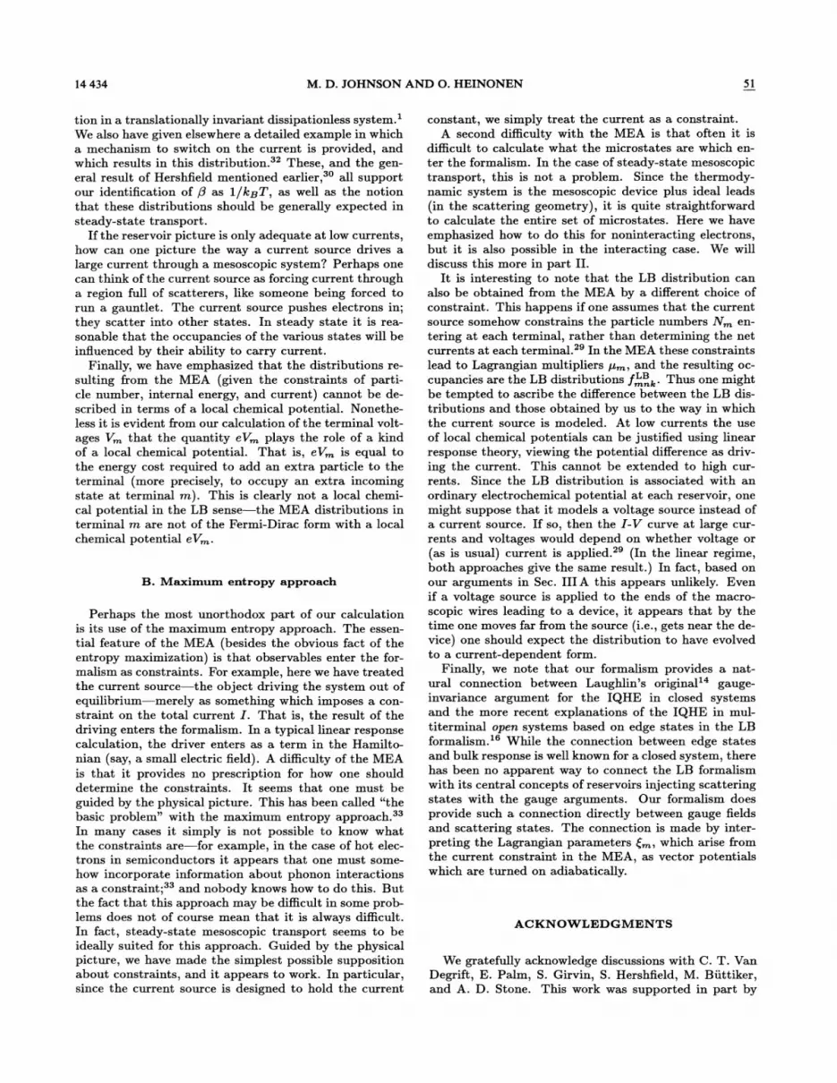
FIG. 1. Schematic energy spectrum of a one-dimensionalmesoscopic device, or a laterally confined two-terminalI+HE system, and zero-temperature occupancies of the sin-gle-particle states in the Landauer-Biittiker picture. In thispicture the occupancies of the states entering the device fromthe source and drain are described by local chemical poten-tials p, and pg, respectively. Occupied states are marked by aheavy line. The asymmetric band bending shown could arisefrom electrostatics, such as a combination of Hall field andconfinement potential in a Hall device. In (a) p, q exceed theminimum of the lowest j subbands (or Landau levels), but liebelow the minimum of the (j + 1)st subband. In (b) y,, (butnot yz) lies above the minimum of the (j + 1)st subband.

the LB approach to give quantization at large currents.The culprit appears to be the very reservoir concept it-self.

Let us examine this in detail, first in an ideal two-terminal example. Denote the minimum energy of thejth subband by Ez. Suppose to begin with that the localchemical potentials of both the source and drain exceedE~ but are less than E~+i. [See Fig. 1(a).] In an idealsystem at zero temperature, the net current in each sub-band is, according to the LB approach, e(p, —pg)/h.(This simple form occurs because of a cancellation be-tween the density of states and the current carried ineach single-particle state. ) With j occupied bands, thisgives a current I = je(p, —p~)/h. The two-terminalvoltage in the reservoir picture is V = (p, —p~)/e, andso the two-terminal resistance is R = V/I = Ii/(je ).

Now let us suppose that the local chemical potential ofthe source (but not of the drain) is increased above E~+i,so that the source injects electrons into the (j + 1)stsubband, while the drain does not. This is shown inFig. 1(b). In an ideal system at zero temperature, thenet current contributed by each of the lower j subbandsis the same as above, but the net current in the (j + 1)st


subband is e(p„—Ez +i.)/h. Thus the total current isI = je(p, —pd)/h+ e(p,, —Ez)/h. The voltage differencemust still be V = (p, —pg)/e in the reservoir picture, so inthis case the LB approach gives a two-terminal resistanceR = V/I which lies between h/(je ) and h/[(j + 1)e j.Notice that this happens whenever one or more of thesubband minima lie between pg and p„which must oc-cur whenever eV exceeds the subband spacing. That is,even in the case of an ideal system, with no backscat-tering, the LB prediction is that the two-terminal resis-tance should not be quantized when eV is large. Andyet in the high-precision IQHE experiments quantizationis found to be extremely accurate even when eV is 10or 100 times the subband spacing. (The same argumenthas been invoked to explain the large-voltage failure ofresistance quantization in quantum point contact exper-iments within the LB formalism. )

The above argument also works in an ideal multiter-rninal IQHE system. Suppose there are four terminals(taken to be identical for simplicity), with two currentterminals 8 and d, and two transverse voltage terminals1 and 2 (see Fig. 2). Then to get zero net current in ter-minal 1, it is necessary that pq

——p, ; similarly, p2 ——pg.A given p, and pg give the same total source-to-draincurrent as above, and the transverse (Hall) voltage is

(pi —p2)/e, also as above. Hence the ideal four-terminalLB results are identical to the ideal two-terminal mea-surements: the resistances are quantized at low but notat high currents.

The discussion thus far has treated the electrons asnoninteracting. With a large current the LB distribu-tion would move many electrons from one edge to theother. Obviously this would have a big electrostatic ef-fect which we have so far neglected but which might re-store quantization. In fact, including electrostatics doesnot help. At the lowest (Hartree) level of approximation,electron-electron interactions can cause the subbands todeviate, perhaps significantly, from the wave number de-pendence which would arise in the noninteracting case.This consequence of electrostatics is pictured schemati-cally in Fig. 1, which shows the bending of energy levels(not too near a contact) in an IQHE sample due to thecombined presence of a Hall 6eld and an edge confine-ment. Of itself, this bending of bands has no e8'ect onthe argument above. If states in one level are occupied

FIG. 2. Schematic representation of a typical four-terminalIQHE device. Current runs along the lower edge from s toterminal 1 and then to d. Similar currents run along the upperedge. If the device is ideal, and all terminals are identical,then in the Landauer-Buttiker picture pq ——p, and pq ——pgto get zero net current in terminals 1 and 2. In the maximumentropy approach under the same circumstances (i ——(, and

out to p,, and pg, then this level contributes e(p, —pg)/hto the current, regardless of the band's shape (becauseof the cancellation between density of states and currentper state). So as long as all subbands shift in energy moreor less together, as is the case with Hartree interactions,the picture is unchanged: a large voltage causes partialoccupancy of higher subbands and hence failure of quan-tization. (We will in part II present detailed numericalcalculations of the electrostatic fields in an ideal Hall barwith a large current. )

Van Son and Klapwijk recently attempted to examinemore closely the consequences of electrostatics for the LBapproach to the IQHE. Their starting point is that elec-tron states (except very close to the current probes) canbe described by bulk Landau levels with a shape givenby a self-consistent electrostatic potential. They arguethat the source injects electrons only in a range of energyp, —4 ( ~ ( p„but that near the source these "relax" tofill (bulk) subbands up to some energy p, ', (with p', ( p, ).For example, when OH = e2/h, after relaxation the low-est subband is filled from pg (for left movers) to p', ( p,(for right movers). Note that, if p', lies above the min-imum of the next subband, this "relaxation" results insome occupied states (e.g. , in the lowest subband) lyingat higher energies than empty states in the next subband.There are two problems with this analysis. First, in amultiterminal device this distribution would be changedat the first voltage probe downstream in some unknownway which one should expect would prevent quantization.Second, Van Son and Klapwijk simply assume that therelaxation process is so eKcient that at low temperaturesstates in the lowest subband end up 6lled continuouslyfrom pg to p', (even though the current source and draindo not directly feed all of them), while the upper sub-bands all are empty (for o~ = e /h). It is difFicult tobelieve that no carriers would end up in any of the highersubbands for large voltages, where p,, —pg is 10 or 100times Lu, . Moreover, this perfect relaxation would haveto suddenly (and inexplicably) end as soon as the drainalso begins inserting carriers directly into the next Lan-dau level, if this is also to explain the IQHE at integersgreater than 1.

Let us turn back to the usual reservoir picture,and examine whether including the interactions moreaccurately by, say, including exchange —can restore thehigh-current quantization. The exchange interaction ef-fectively lowers the energy of the occupied single-particlestates relative to unoccupied states, and in principle thiscould remove the partial occupancy of higher subbands(the cause of the failure to quantize). But the IQHEquantization at large voltages would require the ex-change and correlation energies to exceed 10k' or even100%v, . In fact these energies are much smaller (of or-der 10 bc' ), and it seems implausible that interactionscould restore quantization.

Landauer's insight was that it should be possible toignore the (perhaps very complicated) details of the ter-minals, which are described entirely by the transmissionprobabilities, and concentrate on general principles (see,for example, the discussion in Ref. 10). The existence ofhigh-current quantization in the IQHE and other meso-


scopic devices argues, we believe, that this insight is fun-damentally correct. However, based on the experimen-tal evidence of the high-precision measurements of thequantum Hall resistance, we believe that the model ofterminals as macroscopic reservoirs in local equilibriumis unsatisfactory outside the regime of linear response.Here we will present an approach to mesoscopic transportwhich can be viewed as being within the spirit of Lan-dauer s idea, in that we assume it is possible to neglectthe details of the terminals. Our approach leads, how-ever, to a diferent occupancy of electronic states (andhence requires modification of the reservoir concept), andappears capable of describing transport in mesoscopic de-vices outside of the low-current realm.

II. MAXIMUM ENTROPY APPROACH TOSTEADY-STATE MESOSCOPIC TRANSPORT

We start our approach to steady-state mesoscopictransport with the following fundamental assumption.We assume that the steady state of a mesoscopic sys-tem can be described in terms of an ensemble of electron(or more generally, carrier) states in the mesoscopic de-vice itself. This is analogous to standard assumptions inquantum statistical mechanics in which a system coupledto a heat bath or a particle reservoir can be described byan ensemble average over closed systems in which thecoupling between the particles in the systems and theheat bath or reservoir is not explicitly included, but en-ters only implicitly through Lagrangian multipliers andconstraints. Here, we consider the electron states in asystem with either open or periodic boundary conditions,and do not explicitly include a coupling between the elec-trons and dissipative processes in the terminals. We willalso ignore evanescent modes which decay exponentially&om the terminals.

We will use the maximum entropy approach tononequilibrium statistical mechanics to obtain the dis-tributions over the ensemble of electrons. In this sectionwe will develop our approach to steady-state mesoscopictransport and provide a detailed example which illus-trates how it can explain the I@HE even at large currentsand voltages.

A. Density matrix and current operator

The central ingredient of the maximum entropy ap-proach (MEA) is the information entropy SI. If acomplete set of eigenstates of a thermodynamic systemis labeled by p, then the information entropy is given by

(2)

where P~ is the probability that the system is in a givenmicrostate ~p). Here c is an unspecified constant. (Whenthe MEA is applied to equilibrium thermodynamics, itcan be shown that the information and thermodynamicentropies are identical when c is chosen to be Boltzmann's

constant k~. We will see that this is also true in the caseof steady-state mesoscopic transport. ) As in any thermo-dynamic calculation, the first necessity is to define "thesystem. " We assume that we can define the system to bethe device (including the asymptotic leads), as describedearlier. In general, p then refers to one of a completeset of many-body electron states. In the case of non-interacting electrons each such microstate correspondsto a particular set of occupied single-particle scatteringstates. It is the fact that the device itself is mesoscopicwhich allows for a straightforward description of the mi-crostates. In the presence of dissipation, this is not soeasy. In fact, in spite of claims to its general applica-bility, nearly all applications of the MEA to dissipativenonequilibrium systems have been limited to expansionsabout equilibrium.

The fundamental postulate of the MEA is that theprobabilities P~ are those which maximize the informa-tion entropy —subject to constraints which describe cer-tain given or known observables. The method itself doesnot give a prescription for determining what are the con-straints. These must be determined &om physical con-siderations. (We will discuss this point in more detaillater. ) In the case of equilibrium thermodynamics, it isassumed that the internal energy U and electron numberN can be taken as given, whether or not they are actu-ally measured. In the case of steady-state transport oneknows in addition (by measurement) the net current ateach terminal. We therefore include this as an additionalconstraint and maximize the information entropy subjectto the constraints (H) = U, (N) = N, and (I ) = IHere H is the Hamiltonian, N is the particle numberoperator, and I is an operator giving the net currentin lead m. (We will discuss this operator further be-low. ) These constraints are conveniently imposed usingLagrangian multipliers. The probability entering Eq. (2)can be written as the matrix element P~ = (p~p~p) of thedensity matrix p. Then maximizing Sl subject to theconstraints gives the density matrix

p= exp —P II —pN —) ( I

As in ordinary equilibrium thermodynamics, the La-grangian multiplier associated with the constraint on N isp, the global chemical potential. The intensive variables( are Lagrangian multipliers associated with the con-straints on the currents. Notice that because of currentconservation there are only M —1 independent currentconstraints, and hence one ( can be chosen freely. Itturns out to be convenient to choose (~ = 0, and we doso henceforth. Associated with the constraint on U is theLagrangian multiplier P. In equilibrium P is the inversetemperature; we shall shortly present several argumentswhy this continues to be true here.

For clarity let us begin by considering the case of anideal two-terminal device. This can be either a quasi-one-dimensional conductor, or an ideal Hall bar. We willdiscuss the latter, since the former then follows easily. Inthe two-terminal case we can drop the terminal index m,and understand that k ) 0 (k ( 0) corresponds to states


injected by the source (drain). These can also be calledright and left movers, respectively. In this two-terminalcase the density matrix Eq. (3) becomes

p = exp [—P(H —pN —(I)],

where I measures the current carried &om source todrain. Suppose now that we have noninteracting elec-trons (a restriction which can be removed) in an idealtwo-terminal, two-dimensional strip lying in the xy plane,subject to a magnetic Geld along z. Let x be the longitu-dinal and y the transverse coordinate. The electrons areconfined to the strip by a potential V(y) which, for anideal device, we assume to be a function of the transversecoordinate only. In the Landau gauge A(r) = Byx, the

H= p ——A +Vyn' ('B' B' )+2m* (Bx' By' )+,y' + V(y).

ehBy 8tm c ax

In a nonideal two-terminal system this describes the leadsin the asymptotic region, i.e., away &om the scatteringcenter; there the scattering states @+&(r) have the asymp-totic form

single-particle Hamiltonian is (for charge e electrons ofeffective mass m*)

@.'.(r) =

—k'e '"-'*f„k (y), x -+ oo

1x g

) ('k', k)

n'k'Ie'" f„k (y), x ~ —oo,

n'k'

e* f„„(y)+ ) r(n'k', nk)

with t(n'k', nk) and r(n'k', nk) the transmission and re-Hection amplitudes, respectively. The functions f i, (y)satisfy the Schrodinger equation

(h2k2!( 2m* , -+ 2. .. +V(y) If-~(y)

= e i f i, (y) (7)

j(r) = ) [II;8(r —r, ) + b(r —r;)II;].

Here i labels the particles and II; = p; —eA, /c. Thetotal current passing at x is a result of integrating acrossthe strip:

&(*) = f ~vi-(* u)

&-

[II,.S(~ —*,) + S(~ —~,)ll,.].

and we have adopted the convention that primed summa-tions are restricted to energy-conserving processes, i.e.,e„g = e„g in Eq. (6).

In this paper we will consider only the case of idealsystems, for which r(n'k', nk) = 0 and t(n'k', nk)b„bk k. In this case instead of an infinite system wemay choose a Gnite length L, and impose periodic bound-ary conditions. This replaces the scattering states by@„i,(r) = e'" f„i,(y)/~L. For an ideal system using theperiodic eigenstates gives the same results as the scatter-ing states, but the presentation is simpler.

Next we need to construct the current operator I whichenters Eq. (4). In first-quantized form, the current den-sity operator can be written

I= — dxI x = II; .

In the two-terminal case we can use this as the currentoperator in Eq. (4). The second quantized form of this is

1 .elk„t—:—)Le B2 ) y„ „qc„,„c„i„ (ii)

~~l k

where

y~~~k= dy „~k yy ~k y-

The second-quantized form is more convenient for anopen system, and for an ideal system we can go koma closed to an open system by making the replacement~ P„-+ —,

' jdkIn the absence of an external magnetic Geld, H and I

commute, so the density matrix is diagonal in the diag-onal representation of H. Hence the thermal occupancyof the single-particle state labeled by n, k is given by

f i (() =exp[P(e„k —(i„y —

(M)] + i

Here i i, ——elk/m'L is the current of state nk

In general, matrix elements of I(x) between differ-ent single-particle states have oscillatory components(x exp[i(k —k')x]. Such oscillatory components in the di-agonal elements do not correspond to any net currentthe current carried by a scattering state @„+k(r) in theabsence of a magnetic field is elk/(2am)T A, , where T ),is the total transmission probability for that state. It istherefore useful to define a current operator which is theaverage of I(z) over the length of the device:


In the presence of an external magnetic field, however,H and I do not commute (despite our suggestion to thecontraryi), not even for an ideal system. This imme-diately leads to the apparent problem that the densitymatrix given by Eq. (3) is not stationary, even thoughthe system is in steady state. One possible solution was,given by Grandy, who suggested that, in this case, oneshould include in the constraints only the parts of theoperators which are diagonal in the representation of H.Grandy shows that the diagonal part Fp of an operatorF~ at time t = 0 can in the Heisenberg representationbe written as

The Hamiltonian at t = 0 divers from that at t = —ooby a pure gauge transformation:

H(0) = e' H(—oo)e * (17)

of an integral number of magnetic fiux quanta throughthe center of the system. ) The time-dependent single-particle Hamiltonian under this adiabatic switching on1s

0

Eg = lim g EIr(t)e"'dt,gmo

(14)where

8 = —(2: and ( = e(/RL.

where g is a mathematical infinitesimal. The densitymatrix so constructed is then manifestly time invariantsince it commutes with H.

One could object that this procedure is somewhat adhoc. %le believe that also it is not quite correct, and thatthe correct way to impose a steady-state constraint inthe maximum entropy approach is somewhat subtle inthe presence of a magnetic field. The heart of the prob-lem lies in how the density matrix Eq. (3) can be madestationary, i.e., how one can find a basis in which boththe Hamiltonian H —p,N and the generalized canonicalHamiltonian H (I pN a—re d—iagonal. We will constructsuch a basis by following the procedure of adiabatic turn-ing on, a physically appealing approach. That is, we willturn aside &om the maximum entropy language of con-straints for a while, use adiabatic turning on, and thenshow how the result is connected to Grandy's idea.

We begin by noting that, in first quantization, H —(Ican be written as a sum over single-particle terms of theform

II +V —( II

1 ( e( ) (e(i[II——xi —i

—i

+V (15)2m' ( L y iLy

[using Eqs. (5) and (10)]. This expression is, within anadditive constant, formally identical to adding a puregauge vector potential (c(/L)x to the original Hamilto-nian. Now suppose that c( is an integral number of fiuxquanta (a condition that can be obtained as closely as de-sired for a long system). In this case the vector potential(c(/L)x can be removed by a trivial gauge transforma-tion. From this we conclude that the spectra of H —(Iand H are identical (within an additive constant).

This motivates an important step: let us make thephysical interpretation that the steady state is reachedby adiabatically turning on such an extra vector poten-tial. Do this by switching on a vector potential Ag(t) =—[c((t)/L]x, where ((t) = (g(t) and g(t) is a dimension-less function satisfying g(t -+ —oo) = 0, g(t = 0) = 1,and g'(t = 0) = 0. (This generates the current adiabat-ically via an electric field E = (1/c)BA/Bt which—, forthe periodic system, is caused by the adiabatic insertion

Let U(t2, ti) be the unitary time evolution operator (inthe Schrodinger representation) corresponding to H(t),including the adiabatic evolution of ((t). Then an initialt = —oo single-particle eigenstate ink, —oo) will evolveat t = 0 to ink, 0) = U(0, —oo)ink, —oo). This t = 0state is an eigenstate of H(0). Because of Eq. (17), it isalso the gauge transformation of some other eigenstateof H( —oo):

ink, 0) = e' ]n, k + (,—oo) . (19)

Equation (19) can be shown by noting that (i) the spec-tra of H(0) and H( —oo) are identical; (ii) k is a goodquantum number at both t = —oo and t = 0, and onlythe state with wave vector k + ( on the right-hand sidegives k on the left; and (iii) only one subband can havethe correct energy and wave vector.

To proceed, let us assume that the system reaches equi-librium (at t = —oo) before the current is switched on,and that the system is then thermally isolated while thecurrent is turned on adiabatically. (This is the commonassumption of nonequilibrium statistical mechanics. 2s)Then the final electronic distribution can be describedby an evolved t = 0 density matrix which here, becauseof the equality Eq. (19), can be written in a particularlysimple form using the t = —oo states. To do this let uschange to the language of many-particle states. Definean inital t = —oo ¹ lectron state

iaK¹—oo) = c &(vacuum), (20)

for which

H( (x)))(oKN; —oo) —= &~z~i~KN; —oo). (21)

H(o)I~KN;0) = Z. ~+„,„i~KN; 0). (22)

Here K = g „k, and "occ" signifies a certain setof occupied single-particle states (index a distinguishesamong the difFerent many-particle states with momen-tum K). The time evolution is governed by H(t),which contains the adiabatically changing ((t), and thecorresponding time evolution operator U: icrKN; t)U(t, oo)iaKN; —oo). Be—cause H(0) = e'~H( oo)e '~, —

14 428 M. D. JOHNSON AND O. HEINONEN 51

The expectation value of any operator 0 in theSchrodinger picture at t = 0 can be written

Tr Ot=p pt=p

) (nKN) OlOlnKN; 0)PaKN;0 ~ (23)cxKN

Here P NK;t, = (nKN; tl p(t) lnKN; t) are expectationvalues of the density matrix at time t. The density ma-trix at t = 0 is presumed to be determined by the (equi-librium) density matrix at t = —oo. Hence its t = 0expectation values are simply P KN. 0 ——P KN.

Again using the gauge transformationbetween H( —oo) and H(0), we can thus write Eq. (23)as

0t=P &t=p = oKN;OOoKN;pe ~~

nKN

= ) (n, K + (N, N; —oo le

' Oe* ln, K + (N, N; —oo) eaKN

) (nKN; ool—e ' Oe' laKN; oo)e—aKN

(24)

a,K+Ng', N I

a K+N$ N aKN I0

cr K+N(' N g'(t) dt,—oo

(25)

where we have put (' = (g(t) and g'(t) = dg/dt In the.Schrodinger representation,

(nKN; tl H(t) lnK¹t)

g(l g(l

h,I.(nKN; tlI(t) lnKN; t).

e(26)

The second step follows immediately by inserting thetime-evolution operator, since the contributions kom thederivatives of this operator with respect to (' cancel outin this case. Therefore we can write the thermal averagesin the form

Here e ' Oe' is simply the operator 0 in the gauge inwhich ( has been removed. Hence Eq. (24) shows that we

can write thermal averages in a very simple way by trac-ing over the eigenstates of the original unevolved Hamil-tonian, that is, the Hamiltonian without the current-inducing term ((t). The third form in Eq. (24) is the mostconvenient for calculations in the presence of a magneticfield.

Now let us make one Bnal step which will connect thepreceding to the maximum entropy approach. Rewritethe first of Eqs. (24) using E KN = E K+N& N-(Ea,K+Ng, N

where the subscript H means the Heisenberg representa-tion [ON(t)—:Ut(t, —oo)O(t)U(t, —oo)] and where

0

p(t = 0) = exp —P HN (0) —( IH (t)g'(t) dt

—PNN(0) (28)

EcxKNE,K (N, N= E-aKN

EaKN2! BK2 (29)

For the case of a parabolic confining potential, V(y) =2m*u0y, the single-particle eigenvalues are quadratic ink, and the expansion terminates at the term quadratic in

This density matrix is diagonal in the diagonal represen-tation of the operator in its exponent. This expression issimilar to that given by Grandy [Eq. (14)], and as in thatcase is stationary in this steady-state case. Thus the den-sity matrix Eq. (28) can be obtained using the maximumentropy approach, following a steady-state prescriptionquite similar to Grandy's. However, we note that theadiabatic turning on of the vector potential Ag entersinto the dynamics of the system in a nontrivial way: inEq. (28) the time dependence is given by the Hamilto-nian H(t) in which the adiabatic turning on is included.This apparently technical point is very important to getthe correct answer.

Notice also that we can formally expand E K &N N in

the third of Eqs. (24) in a Taylor series to obtain

Tr 0t=0 pt=p

) (nKN; —oo lOIr (0) laKN; —oo)aKNx(nKN; —oolp(t = 0)laKN; —oo), (27)

E — = E —&I —Na,K (N N aKN ( a—KN 2~eL 2 y + &2y&2

(30)

Thus the density matrix for a quadratic con6ning poten-

51 NONLINEAR STEADY-STATE MESOSCOPIC TRANSPORT: 14 429

tial and a magnetic Geld has the same form as that of asystexn without a magnetic field, and we can in both caseswrite the single-particle occupancies as in Eq. (13).

In suxnmary, the occupancies we obtain depend on thecurrent carried by a state as well as its energy. In theabsence of a magnetic Geld, or with a parabolic confiningpotential, the occupancies for noninteracting electronstake the simple form given by Eq. (13). In the pres-ence of a magnetic field, it is most convenient to use theform shown in the third of Eqs. (24). For noninteractingelectrons this corresponds to occupancies

exp[P(e „~—p)] + 1'

This reduces to Eq. (13) in the absence of a magneticfield, or for the case of a parabolic confining potential.By Eq. (28) this can be seen to be a generalization of thesimple (zero-magnetic-field) result in which the steady-state condition is carefully enforced.

These nonequilibrium distributions in the presence of acurrent are simply a shift of the equilibrium occupancies,which slide over an amount ( in k space. With only onesubband (n = 0) occupied, the single-particle distribu-tions we obtain are similar to those of the LB approach.For example, with zero magnetic field, at zero tempera-

ture, states are occupied up to an energy p+(iok(() (withk here the highest occupied state on an edge). This ispictured in Fig. 3(a). Because the current has oppositesigns for positive and negative A:, right- and left-movingstates are occupied up to different energies. The com-bination p + (iok acts in this case like an effective lo-cal chemical potential. In the general case with severalsubbands occupied, however, states are occupied up todifFerent energies in each subband. [See Fig. 3(b).] Atzero temperature the states in subband n are occupiedup to p + (i k which depends on the current carried bythe highest occupied state in this subband. This currentis in general different in different subbands, and so thedistributions f I, cannot be described in terms of localchemical potentials. Said another way, if one insisted ondefining local chemical potentials, there would need to bea different "local chemical potential" for each subband.

The generalization of these results to the multitermi-nal case is very straightforward and is presented in theAppendix. In the absence of a magnetic field, or fora parabolic confinement, the result is very simple. Inthe multiterminal system the occupancy of the scatter-ing states ~g &) (incoming in terminal m) is given, fornoninteracting electrons, by

exp P Ie „k — ( i~,m~k —p +1

ml

[cf. the corresponding two-terminal expression Eq. (13)].

B. Calculating voltages

(a

Eo

(b

'o

FIG. 3. Current-dependent occupancies of states in anideal two-terminal device, from the maximum entropymethod. Occupied states (at zero temperature) are indicatedby a heavy line. (a) When only one subband is occupied,states are occupied up to energies p+ (ioq. These have dif-ferent values for the outermost occupied states with k ) 0and k ( 0 (shown at k and k', respectively). (b) When morethan one subband is occupied, states in different subbands areoccupied up to different energies. Compare this with Fig. 1.

Within the reservoir model it is quite clear that or-dinary voltage measurements at a contact correspond tothe local chemical potential: V = p /e. (See, for exam-ple, Ref. 16.) As we have emphasized above, the distri-butions derived from the MEA cannot in general be de-scribed in terms of a local chemical potential, and clearlythe LB prescription for finding V cannot apply. Nordoes the MEA itself give some procedure for determin-ing voltages. The approach we take to calculate voltagescomes &om the following physical picture: a voltmeterdetermines the voltage differences between two terminalsby measuring the work required to move a small amountof charge &om one to the other. If moving some chargebQ takes a work hW, then the voltage difference is theratio bW/bQ. The problem is then to calculate this work.

The work required to move reversibly between equilib-rium states is given by changes in thermodynamic po-tentials (e.g. , the Helmholtz &ee energy, when the tem-perature is constant). In general potentials cannot bedefined in nonequilibrium systems, which ordinarily in-volve dissipation. The problem of steady-state trans-port in mesoscopic systems, however, is a special caseof nonequilibrium thermodynamics. In the device thereis no inelastic scattering; this, and the steady-state con-dition, permit us to define thermodynamic potentials of

M. D. JOHNSON AND O. HEINONEN

the electron distribution. For example, the informationentropy is equivalent to an ordinary thermodynamic en-tropy, as mentioned above and explained below; and sohere we can define the Helmholtz 6.ee energy as usual,E = U —TS. The work bW done on the system atconstant temperature is then equal to the change in &eeenergy,

bE= pbN+) ( bI (33)

That is, at constant temperature the Bee energy is a func-tion of the electron number and of the net current at eachterminal. However, the variables most easily varied inthe theory are the intensive variables p, („(i,. . . , (MVarying any of these in general changes the occupancy fof incoining states at each terminal, by Eq. (13). Herefor definiteness we will use the representation given bythe scattering states Iit+ &) labeled by n = mnk, withoccupancies f y In w.hat follows it is useful to define aquantity N which is the number of occupied scatteringstates entering at terminal m. Thus N = P & f I, andthe total electron number in the device is N = P

Let g refer to any of the independent variablesp, („(i,. . . , (M 2. Let bI" denote the change in the netcurrent entering at terminal m when variable g is var-ied while the other independent variables are held fixed.Similarly let bN" be the corresponding change in NThen changing g M g+ bg produces a Bee energy change

we can use eigenstates which satisfy periodic boundaryconditions on a length I. along the device. This particu-lar choice of boundary condition gives a simple density ofstates, but is of no other significance. The states are la-beled by a subband index n and wave vector k. Again inthis case we can drop the terminal subscripts and under-stand that states with k ) 0 are injected by the sourceand k ( 0 by the drain. We choose (~ = 0 and write (for (, . The net current I, entering at the source is justthe total current I through the device. Here we consideronly one simple case, for which the states have energye I, = E + h k /2m' and current i I, = ehk/m*L. Thiscan represent one-dimensional (1D} transport, or a Hallbar with a parabolic transverse confinement. (In the lat-ter case, h /2m* -+ ~OP/2, where uo is the curvature ofthe confining potential and E = ghc/eB is the magneticlength. ) By Eq. (30},the occupancy f i, depends on en-ergy and current in the combination e I, —(i ), . Thisls

h2k2 ehk2m' m'L

h2 ( e( ) e2(2E-+2 . Iik hL)l 2L' (3-7)

Thus the occupancy can be written

f k = f(e ): —P ) =—1/(e '"" " + 1)

bI"" = ) (pbN" +( bI").

%le obtain the potentials V at the terminals by inter-preting this &ee energy change as the work done to addbN I electrons against the voltage V at the terminals.At each terminal the energy cost is ebN" V . Thus wecan also write

where we have defined

h2e„A, ——E„+ (k —(),

e'=hL

(39a)

(39b)

(39c)

8E" =) ebN" V . (35) for reasons which will shortly be apparent. The totalnumber of electrons occupying current-carrying states inthe device is

Equating Eqs. (34) and (35) for each of the M variablesq gives a set of M linearly independent equations,

) b¹(eV —p) = ) ( bI", (36)

C. Ewam. pie

which are to be solved for the unknown terminal voltagesV . The nonlocal resistance measured between two ter-minals m and m' is then R,d, = (V —V )/I. Thematrix bÃ on the left-hand side of Eq. (36) is invertible,and the resulting potentials are then automatically givenrelative to the global chemical potential p.

where in the limit of large I we can take the k's and hencee„A, to be quasicontinuous, and define for the latter a 1Ddensity of states,

p„(e}= (L/~) I2h'(e —E„)/m*] (41)

From the integral form in Eq. (40) we see that N de-pends on )M and ( only in the combination (M given byEq. (39c). Thus here )(J, acts like a current-dependentchemical potential controlling the number of occupiedcurrent-carrying states. The total current carried by theoccupied states is

~ = ) f('- —~) = ) f d.'~-(')f(' P) (4o)—nk n E-

In this section we will illustrate the approach outlinedabove by finding the resistance of an ideal two-terminalsystem, and then extend the result to the ideal multiter-minal case. First consider a two-terminal device. For this

I = ) i„if(e„I —p). (42)

Notice that f I, is symmetric about k = (. That is, the

NONLINEAR STEADY-STATE MESOSCOPIC TRANSPORT:

two states in subband n at k~ = (+ [2m'(e —E )/h2] ~

have the same value of e A, = e and hence, Rom Eq. (38),the same occupancy. The current carried by these twostates is then

i (k+) +i (k ) = eh(k+ + k )/m*L = 2eh(/m*L.

(43)

where e„& ——E„+h (k —( —b() /2m*. Since e & issymmetric about ( + b(, the only contribution to thesum over k is for ( ( k & ( + 2b(, so that

6+2~4

bq ) ) eP(~ ~—~—sP)+y

Thus the total current is(49)

.L).f(e i —p) = (44)

With these expressions it is new straightforwardto compute the current-voltage relations by invertingEqs. (36). In this two-terminal example, it is easier to use

p and ( as independent variables instead of the originalpair p, (. Then for this example there are two Eqs. (36),labeled by g = p, , (:

plus terms of second order in the quantities b( and bp.That is, b Q~ = b Q and b Q" = 0. From the expressionfor N given in Eq. (40) it is evident that varying ( andp, changes N by

(bNI" bÃd \ / eV, —y, & bI" lI bN( bN& ) (eV„—pp bI

that is, bÃ" = bN and bN& = 0. Combining Eqs. (50),(49), and (47), we find

These equations contain bN", the change in the occupa-tion number N of states which carry current into ter-minal m. We are interested in the changes in these whichresult when i) = (, P are changed infinitesimally. Ratherthan computing these directly, consider a function

PNP gyP

bNt = —bN,' = -bq.

From Eq. (44) we obtain

(5i)

Q(p, , (; kp) = ) f(e„i, —p, )sgn(k —kp). (46)

Notice that Q depends on ( via e i„which, by Eq. (39a),depends on (. The quantity 2 (N + Q) gives the numberof occupied states with k ko. We ultimately seek thechanges in the number of occupied states with k 0 due

to infinitesimal changes bp, and b(. But the changes inoccupation of these states are the same as the changes inoccupation numbers of states with k ko, as long as ko isnot too close to the edge of occupied k's (that is, as longas states near wave number ko are either fully occupiedor unoccupied). Thus we can write

bN,"~ = (bN" + bQ"), —1(47)

bQ = Q(p+ bp, (+ b( ()

sgn(k — ),nk

(48)

where the upper (lower) sign is for m = s (d), and qrepresents variations in either p or (. Let us choose kp ——

[Then, more precisely, Eq. (47) is true as long as theregion of k space where f (e i, P) is very c—lose to unity (atlow temperatures) brackets both ( and k = 0. This willbe discussed further in part II, since this point leads toa breakdown in quantization in point contacts. ] Clearly

Q(p, , (;kp ——() = 0. We seek

bI" = (bÃ,m*L

(52)

G= I/(V, —Vg) = —) ( )(53)

If p, exceeds the band minima of the first j subbands (orLandau levels), then at low temperatures G = je2/h.Finite-temperature corrections are exponentially small.This quantization occurs because at large currents it isquite possible for states in one subband to be occupiedup to energies above those of empty states in other sub-bands [as pictured in Fig. 3(a)]—not because relaxationhas failed to occur, but because according to the MEAthis is the steady-state (although highly nonequilibrium)result.

This exact result is true for an ideal system with aparabolic energy spectrum. We emphasize that this ex-ample is special only in that it can be solved analytically(which is the reason we have used it to illustrate ourmethod). We have numerically studied nonparabolic en-ergies e y and multiterminal systems, and And in thesecases that the accuracy of quantization is limited only by

It is now a simple matter te invert the matrix inEq. (45) and solve for V, d. We write the final answeras the two-terminal conductance


the numerical accuracy. In our method zero-temperaturequantization persists up to very high currents and volt-ages. Quantization can fail when the current grows solarge that a subband is occupied only for carriers mov-ing in one direction. This is similar to the distributionsfor which the LB approach fails to give quantization [asin Fig. 1(b)]. But it is important to emphasize that theconditions under which this failure of quantization oc-curs are very di8'erent in the two cases. In our approach,increasing the current shifts the occupancy of states in asubband (at zero temperature) from left movers to rightmovers. In IQHE devices one should expect the sub-bands to look schematically like those in Figs. I and 3: arelatively fIat "bulk" region surrounded by edge regionswhere the energy increases rapidly. As long as the densityof bulk states greatly exceeds that of edge states, one canpush the energy of the highest-occupied right movers veryhigh while left movers in the same subband are occupied.In the LB approach, on the other hand, a subband im-mediately becomes partially occupied. as soon as p,, butnot pg exceeds the subband's minimum [as in Fig. 1(b)].This occurs whenever eV~ exceeds the subband spac-ing. In our approach, instead, it is quite possible [as inFig. 3(a)] for states in a lower subband to be occupiedto energies above vacant states in a higher subband. Toempty the left movers in a subband would generally re-quire quite high currents and voltages in our approach.How high the voltage can get depends on the ratio of thenumber of current-carrying states in the relatively 8atportion of the band to those in the steep edge region.This should be quite high in typical Hall devices. In theparticular case of a parabolic energy spectrum, however,left movers wouM be d.rained at relatively low voltages(eV~ of order 2Ru, ). This is not relevant to Hall devices,but is relevant to experiments in quasi-one-dimensionalsystems such as quantum point contacts, and to the sat-uration observed there. This will be discussed furtherin part II. Exceptions to quantization can also occur inour approach when the current is large enough to inducebreakdown in the sample as a consequence of other dis-sipative mechanisms. For ordinary samples exhibitingthe IQHE, neither this nor the earlier possibility occurs,and our approach described above provides an explana-tion of the extremely accurate quantization observed out-side the linear response regime. This ability to explainthe high-precision IQHE experiments is nontrivial, andlends credence to the postulate of the MEA.

The above example was explained in detail to showhow our approach is applied in general. In this partic-ular case of a two-termina1 system, a simplification ispossible. Since N depends on p, and not $, changing thelatter while holding the former constant corresponds tomoving a charge ehQ/2 from one terminal to the other(or from edge to edge in a quantum Hall sample). Thework required to do this (at constant 1V) is bE~ = (bI~.Hence the voltage difI'erence is

e(V, —Vg) =

which gives the same result.

III. DISCUSSION

A. Density matrix

The density matrix and distribution which result fromthe maximum entropy approach, and which lie at theheart of our ability to explain the high-precision IQHEexperiments, are unusual, but not unheard of in the lit-erature. The distribution f in Eq. (13) was proposedearlier by Heinonen and Taylor, and more recently byNg. These authors argued that in a device withoutdissipation it should be possible to de6ne a &ee energywhich, presuxnably, would be minimized. The process ofminimization, subject to the current constraint, is for-mally identical to the MEA s maximization of informa-tion entropy, and leads to the same distribution. In thispaper we have obtained this result on considerably morefundamental grounds —assuming only the postulates ofthe maximum entropy approach to nonequilibrium sta-tistical mechanics are, in fact, correct.

Here we will seek some understanding of the densitymatrix Eq. (3) and distribution Eq. (13) &om other view-points. Note first of all that this density matrix has thegeneral form which Hersh6eld recently showed should ex-ist on quite general grounds in steady-state nonequilib-rium systems. In his rather more conventional approachto nonequilibrium statistical mechanics, it is quite ev-ident that P in Eq. (13) is indeed 1/k~T, where T isthe texnperature. This was not obvious in the MEA, butbased on Hershfield's work we can make the same identi-fication, in the case of steady-state mesoscopic transport.It also then follows that the information and thermody-namic entropies are equivalent [with c in Eq. (2) set tokg].

The distributions Eq. (13) are obviously quite differ-ent from the LB distributions. The latter follow in a verystraightforward way &om the model of terminals as reser-voirs, and are widely considered valid by their ability todescribe nonlocal resistances in many low-current exper-iments, as well as by the appealing simplicity and clarityof the reservoir model itself. How can this difference indistributions be understood physically'? The LB distribu-tions can be derived &om linear response theory, with acertain assumption about how the system is driven. Onecan apply something very similar to the reservoir idea ina very precise calculation by modeling the leads as idealand supposing that far &om the device there is in eachlead a well-defined electrochemical potential. Stone andco-workers have shown that this assumption leads in lin-ear response to the multiterminal LB formalism. "' Weshould note, however, that this work has been criticizedby Landauer, based on their use of leads of constant crosssection, which do not have the geometrical spreading hebelieves is necessary for the reservoir picture. Even so,while indeed no large reservoir is invoked in the work ofStone et al. , a very similar idea—that far &om the de-vice a probe can be described as a system at constantpotential —is at the heart of this calculation, entering asa boundary condition. (We should also note that, sincein principle linear response can be calculated using equi-

51 NONLINEAR STEADY-STATE MESOSCOPIC TRANSPORT: 14 433

Of Bk Of (df tv +

Bx Bt Bk (dt) (55)

We want the lowest-order (in b,p) solution to this, in therelaxation time approximation. Since the conductor' sends are held at definite local chemical potentials, thedistribution takes the LB form at the ends:

librium distributions, the success of the linear theory inpredicting low-current properties does not imply that thelinear distributions are correct. )

We emphasize that built into Stone et al. 's and relatedcalculations is the model of terminals as entities describedby local chemical potentials. This model fits neatly intothe most common way to approach nonequilibrium prob-lems: assuming that there are two large reservoirs, eachin equilibrium, and that transport (say) between themoccurs when they are connected by a small channel. Thisis a very familiar approach to nonequilibrium statisti-cal mechanics. And yet it amounts to an assumption asto how the system is driven. In typical transport ex-periments in the I@HE, say, a constant current sourceis connected to the sample. Using the reservoir pictureamounts to a model of how a current source (when con-nected to a mesoscopic device) actually drives the cur-rent. Perhaps it is valid in linear response to model thecurrent source as two leads at different potentials. Evenif valid in linear response, it is not a priori clear thatthe picture should be valid at large currents. In fact, thefailure of the LB approach at large currents suggests not.

Let us examine this in more detail. Suppose thatthe current source itself can be viewed as an objectwhich gives rise to different potentials in the physicalleads. Then the current is carried down long macroscopiclengths of lead until it is injected. into the device throughthe terminals. Perhaps along the macroscopic wire thelocal potential changes gradually and smoothly (due toelastic and inelastic scattering); that is, perhaps the dis-tribution locally can be described by a local chemicalpotential. Does this picture work right up to the vicin-ity of the mesoscopic device? In fact, there are severalreasons to think not.

The simplest way to approach this is in the approxima-tion of the Boltzmann approach to transport. Consideran ordinary dissipative conductor carrying a low current.Let us suppose that the current is driven by reservoirsheld at two different potentials. Then at the reservoirsthe Boltzmann distribution f(r, k, t) will have the LBform. But a perfectly standard Boltzmann calculationshows that far from the reservoirs the distribution evolvesinto a current-dependent form identical (in first order) tothat derived &om the MEA [Eq. (13)],and different &omthe first-order LB distributions. Suppose that the ends ofan efFectively one-dimensional conductor (at z = +L/2)are held at difFerent electrochemical potentials p + b,p/2.The distribution is then labeled by a wave number k plusa subband index n: f = f(z, n, k, t) Suppose fur. therthat this gives rise to a uniform electric field E = b, IJ/eLthrough the conductor. Then in steady state and onedimension the Boltzmann equation becomes

f(pL/2, n, k, t) = 1/(exp(P[e„A, —(p 6 b.p/2)]) + 1).

(56)

The upper sign is for positive k and the lower for negativek. Equation (55) is a completely standard Boltzmannproblem, with the only wrinkle provided by the bound-ary conditions, Eq. (56). To linear order this problem issolved by

Bfo,f &km 11, ( ~gy2)ysg Skago+ &POe (mL 2) mL

(57)

where again the upper (lower) sign is for k ) 0 (k ( 0).Here fp(e &) = 1/(e~~ "' ~l + 1) is the equilibrium dis-tribution and w is the relaxation time (which can dependon k). Let us suppose that the relaxation time w is muchless than the transit time across the system: 7 « I/v,where the speed v = hk/m. Then at distances muchfarther than v~ &om the ends the distribution becomes

f =fo ~b p. Bfp&nk (58)

Here i i, = ev/I is the current carried by the state insubband n with wave vector k. Equation (58) is thelowest-order term in an expansion in current of

1

exp[P(e„I, —p —(i„A,)] + 1'

where we have here identified ( =

&ATE/e.

Note that thisis not equal to the corresponding first-order LB distribu-tion f = fp ~ (Ap/2)Bfp/Be

That is, in a completely typical dissipative conduc-tor, the Boltzmann distribution is precisely the lowest-order approximation to the distribution [Eq. (13)] ob-tained &om the maximum entropy calculation. This isthe case even though we chose the boundaries to modelreservoirs; the distribution evolves &om the LB formnear the ends to the current-dependent form away Romthe ends. Our point with this exaxnple is the following.Even though the LB distribution has the authority ofwidespread usage, perhaps one should instead typicallyexpect to find current-dependent distributions carryingsteady-state currents into a mesoscopic system; for thedissipative wires carrying the current to the mesoscopicdevice should themselves typically have such distribu-tions. Note that the Boltzmann equation gives current-dependent distributions also in the familiar case of athree-dimensional conductor in the relaxation time ap-proximation. In this case the resulting distribution isobtained by displacing the Fermi surface in the directionof the current, and therefore here too the occupancy ofsingle-particle states depends on their current as well astheir energy.

There are special cases in which current-dependent dis-tributions can be obtained in other ways. We have arguedelsewhere that this should arise by Galilean transforma-


tion in a translationally invariant dissipationless system.We also have given elsewhere a detailed example in whicha mechanism to switch on the current is provided, andwhich results in this distribution. These, and the gen-eral result of Hershfield mentioned earlier, all supportour identification of P as 1/k~T, as well as the notionthat these distributions should be generally expected insteady-state transport.

If the reservoir picture is only adequate at low currents,how can one picture the way a current source drives alarge current through a mesoscopic system'? Perhaps onecan think of the current source as forcing current througha region full of scatterers, like someone being forced torun a gauntlet. The current source pushes electrons in;they scatter into other states. In steady state it is rea-sonable that the occupancies of the various states will beinQuenced by their ability to carry current.

Finally, we have emphasized that the distributions re-sulting from the MEA (given the constraints of parti-cle number, internal energy, and current) cannot be de-scribed in terms of a local chemical potential. Nonethe-less it is evident from our calculation of the terminal volt-ages V that the quantity eV plays the role of a kindof a local chemical potential. That is, eV is equal tothe energy cost required to add an extra particle to theterminal (more precisely, to occupy an extra incomingstate at terminal m). This is clearly not a local chemi-cal potential in the LB sense —the MEA distributions interminal m are not of the Fermi-Dirac form with a localchemical potential eV

B. Maximum entropy approach

Perhaps the most unorthodox part of our calculationis its use of the maximum entropy approach. The essen-tial feature of the MEA (besides the obvious fact of theentropy maximization) is that observables enter the for-malism as constraints. For example, here we have treatedthe current source —the object driving the system out ofequilibrium —merely as something which imposes a con-straint on the total current I. That is, the result of thedriving enters the formalism. In a typical linear responsecalculation, the driver enters as a term in the Hamilto-nian (say, a sinall electric field). A difficulty of the MEAis that it provides no prescription for how one shoulddetermine the constraints. It seems that one must beguided by the physical picture. This has been called "thebasic problem" with the maximum entropy approach.In many cases it simply is not possible to know whatthe constraints are—for example, in the case of hot elec-trons in semiconductors it appears that one must some-how incorporate information about phonon interactionsas a constraint; and nobody knows how to do this. Butthe fact that this approach may be diKcult in some prob-lems does not of course mean that it is always diFicult.In fact, steady-state mesoscopic transport seems to beideally suited for this approach. Guided by the physicalpicture, we have made the simplest possible suppositionabout constraints, and it appears to work. In particular,since the current source is designed to hold the current

constant, we simply treat the current as a constraint.A second difBculty with the MEA is that often it is

diKcult to calculate what the microstates are which en-ter the formalism. In the case of steady-state mesoscopictransport, this is not a problem. Since the thermody-namic system is the mesoscopic device plus ideal leads(in the scattering geometry), it is quite straightforwardto calculate the entire set of microstates. Here we haveemphasized how to do this for noninteracting electrons,but it is also possible in the interacting case. We willdiscuss this more in part II.

It is interesting to note that the LB distribution canalso be obtained from the MEA by a difFerent choice ofconstraint. This happens if one assumes that the currentsource somehow constrains the particle numbers N en-tering at each terminal, rather than determining the netcurrents at each terminal. In the MEA these constraintslead to Lagrangian multipliers p, and the resulting oc-cupancies are the LB distributions f"B&. Thus one mightbe tempted to ascribe the difference between the LB dis-tributions and those obtained by us to the way in whichthe current source is modeled. At low currents the useof local chemical potentials can be justified using linearresponse theory, viewing the potential difference as driv-ing the current. This cannot be extended to high cur-rents. Since the LB distribution is associated with anordinary electrochemical potential at each reservoir, onemight suppose that it models a voltage source instead ofa current source. If so, then the I-V curve at large cur-rents and voltages would depend on whether voltage or(as is usual) current is applied. (In the linear regime,both approaches give the same result. ) In fact, based onour arguments in Sec. IIIA this appears unlikely. Evenif a voltage source is applied to the ends of the macro-scopic wires leading to a device, it appears that by thetime one moves far &om the source (i.e. , gets near the de-vice) one should expect the distribution to have evolvedto a current-dependent form.

Finally, we note that our formalism provides a nat-ural connection between Laughlin's original gauge-invariance argument for the IQHE in closed systemsand the more recent explanations of the IQHE in mul-titerminal open systems based on edge states in the LBformalism. While the connection between edge statesand bulk response is well known for a closed system, therehas been no apparent way to connect the LB formalismwith its central concepts of reservoirs injecting scatteringstates with the gauge arguments. Our formalism doesprovide such a connection directly between gauge fieldsand scattering states. The connection is made by inter-preting the Lagrangian parameters (, which arise &omthe current constraint in the MEA, as vector potentialswhich are turned on adiabatically.

ACKNOWLEDGMENTS

VA gratefully acknowledge discussions with C. T. VanDegrift, E. Palm, S. Girvin, S. Hershfield, M. Buttiker,and A. D. Stone. This work was supported in part by


the UCF Division of Sponsored Research, and by theNational Science Foundation under Grant No. DMR-9301433.

APPENDIX: DISTRIBUTIONS FORMULTITERMINAL SYSTEMS

he -t

e2B+

2m. m*c ~:nn'

m" =m' (A5)

Atdk I um, n', n, k~~nrkcmnk &

m".m =I'7 ) fdkkc „&c a, m"=m, (Al)

and

1m .m=- dkkct „c „„, m" = m',27rm* mnk n»

n

(A2)

and zero otherwise. Just as in the two-terminal case, thedensity matrix then commutes with the Hamiltonian Hand one can immediately write down the single-particleoccupation numbers in terms of the diagonal elements&mnk an& &mnk ~

For a multiterminal device in the presence of an exter-nal magnetic field, we start by choosing a gauge in whichthe vector potential is a Landau gauge in all leads,

It is straightforward to generalize our formalism toopen ideal multiterminal devices in the absence of an ex-ternal magnetic field. We define coordinates (x, y )such that x points into the device in lead m, andx x y = z; the confining potential V(r) (which definesthe geometry) can asymptotically in lead m be writtenV(y ). In an ideal system, all states injected into leadm reach only the terminal at the lead m', say, and wedefine the operator for incoming current in lead m" ofstates injected into lead m as

and zero otherwise. The generalized canonical Hamilto-nian II —P ( I —pN, which determines the densitymatrix, is in the asymptotic regions in lead m equivalentto a Hamiltonian given in first quantization by

I . —„2 52(2H= ) II, —Q x — +V(y ), (A6)

with

e m

2mb(A7)

II= ) ( II, ——) Ag (t, r, ) +V(r, ) &,

Thus ( enters as a vector potential in lead m. We thensmoothly continue ( x to a divergenceless irrotationalvector function (r) in all space which is equal to ( xasymptotically in lead m, —( x ~ asymptotically in leadm' (as defined above), and zero in the asymptotic re-gions in all other leads. A suitable analogy would be tothink of (r) as the velocity field of an incompressibleQuid which Qows irrotationally in through lead vn andout through lead m'. We then turn on the vector poten-tials adiabatically by taking ( ~ g g(t) and study thetime-dependent system with the Hamiltonian

A(r) = By x (A3) (A8)

) dk kct „qc

e2B2+m*c

nn'

p, td~ ~gm, nl, n, k~~ lk~mnk~

m" = m, (A4)

with x in the asymptotic region in lead m. States in-jected into lead m now all exit the system at the nextlead m' defined by the direction of the magnetic field.For example, in Fig. 2, if the source is terminal m, thenterminal 1 in that figure would correspond to m', and soon. We define the current operator for current in leadm" of states injected into lead m as

where At (t, r) = —(ch/e) (t, r). Just as in the idealtwo-terminal case, adiabatically turning on the vector po-tentials &om t = —oo will then generate a system at t = 0with net currents. Here, the parameters ( have to bethought of as adjustable parameters, adjusted to give thecorrect net currents at each terminal. As an example,consider an ideal multiterminal I@HE system. Supposethere are four identical terminals, as shown in Fig. 2.Then all of the current leaving the source Qows along thelower edge to terminal 1. For the net current throughterminal 1 to vanish, it is necessary that (i ——(, . Simi-larly, (2 ——(g = 0. The work required to transfer a certaincharge &om terminal 1 to 2 is then precisely that requiredto move the same charge &om 8 to d in the two-terminalcalculation. Hence the two-terminal conductance calcu-lated above becomes here the Hall conductance, which isthen quantized.


O. Heinonen and M.D. Johnson, Phys. Rev. Lett. 71, 1447(1993).K. von Klitzing, G. Dorda, and M. Pepper, Phys. Rev.Lett. 45, 494 (1980); K. von Klitzing, Rev. Mod. Phys. 58,519 (1986); see also The Quantum Hall Effect, edited byR.E. Prange and S.M. Girvin (Springer-Verlag, New York,1987).For example, the GaAs heterojunction used to maintain theresistance standard at the U.S. National Institute of Stan-dards and Technology shows quantization to better thanone part per billion at the v = 4 plateau for eVH ) 16~ .See, for example, J.J. Palacios and C. Tejedor, Phys. Rev.B 44, 8157 (1991).R. Landauer, IBM J. Res. Dev. 1, 223 (1957); Philos. Mag21, 863 (1970); Z. Phys. B 21, 247 (1975); 68, 217 (1987).M. Biittiker, Phys. Rev. Lett. 5'7, 1761 (1986); Phys. Rev.B 38, 9375 (1988); IBM J. Res. Dev. 32, 317 (1988).A.D. Stone and A. Szafer, IBM J. Res. Dev. 82, 384 (1988).H.U. Baranger and A.D. Stone, Phys. Rev. B 40, 8169(1989).P.C. van Son and T.M. Klapwijk, Europhys. Lett. 12, 429(1990).R. Landauer, in Analogies in Optics and Micro Electron-ics, edited by W. van Haeringen and D. Lenstra (Kluwer,Dordrecht, 1990), p. 243; Phys. Scr. T42, 110 (1992).See, for example, Quantum Transport in Semiconductors,edited by D.K. Ferry and C. Jacoboni (Plenum, New York,1992).E.T. Jaynes, Phys. Rev. 106, 620 (1957); 108, 171 (1957).For recent treatments, see, for example, W.T. Grandy, Jr. ,in Foundations of Statistica/ Mechanics (Reidel, Dordrecht,1988), Vols. 1 and 2; H. S. Robertson, Statistical Thermophysics (Prentice-Hall, Englewood Cliffs, NJ, 1993).Electron-electron interactions may be included in general.R.B. Laughlin, Phys. Rev. B 23, 5632 (1981).Y. Imry, in Directions in Condensed Matter Physics, editedby G. Grinstein and G. Mazenko (World Scientific, Singa-pore, 1986), p. 101.

For a review of the Landauer-Biittiker approach in the con-text of the quantum Hall effect, see M. Biittiker, in Nano-structured Systems (Ref 3. 4), Chap. 4, p. 191.F. Sols, Ann. Phys. (N.Y.) 214, 386 (1992).A.M. Kriman, N.C. Kluksdahl, and D.K. Ferry, Phys. Rev.B 86, 5953 (1987).Note that in this somewhat unfortunate, but standard,notation the field creation operator is written vent(r)

E ., (~ .,)'()".,P. Streda, J. Kucera, and A.H. MacDonald, Phys. Rev.Lett. 59, 1973 (1987); J.K. Jain and S.A. Kivelson, ibid.60, 1542 (1988); Phys. Rev. B 37, 4276 (1988).M. Biittiker, in I'eskorperprobleme. Advances in Solid StatePhysics, edited by F. V. Braunschweig (Pergamon, Oxford,1990), Vol. 30, p. 41.U. Sivan and Y. Imry, Phys. Rev. B 33, 551 (1986).B.I. Halperin, Phys. Rev. B 25, 2185 (1982).H. van Houten, C.W.J. Beenakker, and B.J. van Wees, in1Vanostructured Systems (Ref. 34).For a clear statement about this point, see J. Rammer andH. Smith, Rev. Mod. Phys. 58, 323 (1986).More general circumstances under which thermodynamicpotentials can be defined out of equilibrium have been con-sidered by R.J. Tykodi, Thermodynamics of Steady State(Macmillan, New York, 1967).M. Cage et al. , Phys. Rev. Lett. 51, 1374 (1983).O. Heinonen and P.L. Taylor, Phys. Rev. 8 28, 6119(1982); 82, 633 (1985).T.K. Ng, Phys. Rev. Lett. 68, 1018 (1992).S. Hershfield, Phys. Rev. Lett. 70, 2134 (1993).G.D. Mahan, Many Particle -Physics, 2nd ed. (Plenum,New York, 1990), Chap. 7, p. 602.O. Heinonen and M.D. Johnson, Phys. Rev. B 49, 13740(1994).R. Landauer, Physica A 194, 551 (1993).Nanostructured Systems, edited by M. Reed, Semiconduc-tors and Semimetals Vol. 35 (Academic Press, New York,1992).

Documents

Nonlinear Steady-State Mesoscopic Transport, I. Formalism