Nonlinear System Identification Using Exponential Swept-Sine Signal

IEEE TRANSACTIONS ON INSTRUMENTATION AND MEASUREMENT 1

Nonlinear System Identification UsingExponential Swept-Sine Signal

Antonín Novák, Laurent Simon, Member, IEEE, František Kadlec, and Pierrick Lotton

Abstract—In this paper, we propose a method for nonlin-ear system (NLS) identification using a swept-sine input signaland based on nonlinear convolution. The method uses a non-linear model, namely, the nonparametric generalized polynomialHammerstein model made of power series associated with linearfilters. Simulation results show that the method identifies thenonlinear model of the system under test and estimates the linearfilters of the unknown NLS. The method has also been tested on areal-world system: an audio limiter. Once the nonlinear model ofthe limiter is identified, a test signal can be regenerated to comparethe outputs of both the real-world system and its nonlinear model.The results show good agreement between both model-based andreal-world system outputs.

Index Terms—Analysis, generalized polynomial Hammersteinmodel, identification, nonlinear convolution, nonlinear system(NLS), swept-sine.

I. INTRODUCTION

THE theory of linear time-invariant (LTI) systems has beenextensively studied over decades [1], [2], and the estima-

tion of any unknown LTI system, knowing both the input andoutput of the system, is a solved problem. The fundamentalidea of the theory states that any LTI system can be charac-terized entirely by its impulse response in the time domain orby its frequency response function in the frequency domain.Nevertheless, almost all real-world devices exhibit more or lessnonlinear behavior. In the case of very weak nonlinearities,a linear approximation can be used. If the nonlinearities arestronger, the linear approximation fails, and the system has to bedescribed using a nonlinear model. Such nonlinear models areavailable in the literature, e.g., the Volterra model [3], the neuralnetwork model [4], the multiple-input–single-output (MISO)model [5], the nonlinear autoregressive moving average withexogenous inputs model [6], [7], the hybrid genetic algorithm[8], extended Kalman filtering [9], and particle filtering [10].

Manuscript received July 21, 2008; revised August 14, 2009; acceptedAugust 14, 2009. This work was supported in part by the Ministry of Educationof Czech Republic under the research program “Research in the Area ofthe Prospective Information and Navigation Technologies” under ContractMSM6840770014 and in part by the French Embassy in Prague within theframework of the program “Cotutelle de thèse.” The Associate Editor coor-dinating the review process for this paper was Dr. Jesús Ureña.

A. Novák is with Laboratoire d’Acoustique de l’Université du Maine,Unite Mixte de Recherche-Centre National de la Recherche Scientifique(UMR-CNRS) 6613, 72085 Le Mans, France, and also with the Faculty ofElectrical Engineering, Czech Technical University, Prague 166 27, CzechRepublic (e-mail: [email protected]).

L. Simon and P. Lotton are with Laboratoire d’Acoustique de l’Université duMaine, UMR-CNRS 6613, 72085 Le Mans, France.

F. Kadlec is with Faculty of Electrical Engineering, Czech Technical Univer-sity, Prague 166 27, Czech Republic.

Digital Object Identifier 10.1109/TIM.2009.2031836

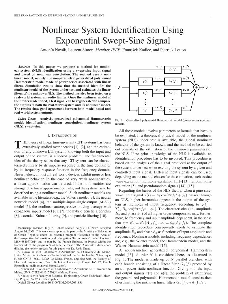
Fig. 1. Generalized polynomial Hammerstein model (power series nonlinearmodel).

All these models involve parameters or kernels that have tobe estimated. If a theoretical physical model of the nonlinearsystem (NLS) under test is available, the global nonlinearbehavior of the system is known, and the method to be carriedout consists of the estimation of the unknown parameters ofthe NLS. If no prior knowledge of the NLS is available, anidentification procedure has to be involved. This procedure isbased on the analysis of the signal produced at the output ofthe system under test when exciting the system by a given andcontrolled input signal. Different input signals can be used,depending on the method chosen for the estimation, such as sinewave excitation, multitone excitation [11]–[13], random noiseexcitation [5], and pseudorandom signals [14], [15].

Regarding the basics of the NLS theory, when a pure sine-wave input signal x(t) = A1 cos(2πf1t + φ1) passes throughan NLS, higher harmonics appear at the output of the sys-tem as multiples of input frequency, according to y(t) =∑

n Bn cos(2πnf1t + φn). The characteristics (i.e., amplitudeBn and phase φn) of all higher order components may, further-more, be frequency and input amplitude dependent, in the sensethat ∀n Bn ≡ Bn(A1, f1), φn ≡ φn(A1, f1). The completeidentification procedure consequently needs to estimate theamplitude Bn and phase φn as functions of input amplitude andfrequency. Nonlinear models, including frequency dependence,are, e.g., the Wiener model, the Hammerstein model, and theWiener–Hammerstein model [15].

A nonparametric generalized polynomial Hammersteinmodel [15] of order N is considered here, as illustrated inFig. 1. The model is made up of N parallel branches, witheach branch consisting of a linear filter Gn(f) preceded byan nth power static nonlinear function. Giving both the inputand output signals x(t) and y(t), the problem of identifyingthe generalized polynomial Hammerstein model consists thenof estimating the unknown linear filters Gn(f), n ∈ [1, N ].

0018-9456/$26.00 © 2009 IEEE

2 IEEE TRANSACTIONS ON INSTRUMENTATION AND MEASUREMENT

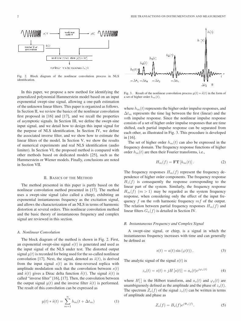
Fig. 2. Block diagram of the nonlinear convolution process in NLSidentification.

In this paper, we propose a new method for identifying thegeneralized polynomial Hammerstein model based on an inputexponential swept-sine signal, allowing a one-path estimationof the unknown linear filters. This paper is organized as follows.In Section II, we review the basics of the nonlinear convolutionfirst proposed in [16] and [17], and we recall the propertiesof asymptotic signals. In Section III, we define the swept-sineinput signal, and we detail how to design this input signal forthe purpose of NLS identification. In Section IV, we definethe associated inverse filter, and we show how to estimate thelinear filters of the model. In Section V, we show the resultsof numerical experiments and real NLS identification (audiolimiter). In Section VI, the proposed method is compared withother methods based on dedicated models [25], such as theHammerstein or Wiener models. Finally, conclusions are notedin Section VII.

II. BASICS OF THE METHOD

The method presented in this paper is partly based on thenonlinear convolution method presented in [17]. The methoduses a swept-sine signal (also called a chirp), exhibiting anexponential instantaneous frequency as the excitation signal,and allows the characterization of an NLS in terms of harmonicdistortion at several orders. This nonlinear convolution methodand the basic theory of instantaneous frequency and complexsignal are reviewed in this section.

A. Nonlinear Convolution

The block diagram of the method is shown in Fig. 2. First,an exponential swept-sine signal s(t) is generated and used asthe input signal of the NLS under test. The distorted outputsignal y(t) is recorded for being used for the so-called nonlinearconvolution [17]. Next, the signal, denoted as s(t), is derivedfrom the input signal s(t) as its time-reversed replica withamplitude modulation such that the convolution between s(t)and s(t) gives a Dirac delta function δ(t). The signal s(t) iscalled “inverse filter” [16], [17]. Then, the convolution betweenthe output signal y(t) and the inverse filter s(t) is performed.The result of this convolution can be expressed as

y(t) ∗ s(t) =∞∑

m=1

hm(t + Δtm) (1)

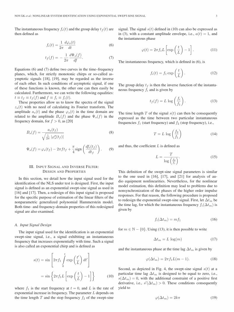
Fig. 3. Result of the nonlinear convolution process y(t) ∗ s(t) in the form ofa set of higher order hm(t).

where hm(t) represents the higher order impulse responses, andΔtm represents the time lag between the first (linear) and themth impulse response. Since the nonlinear impulse responseconsists of a set of higher order impulse responses that are timeshifted, each partial impulse response can be separated fromeach other, as illustrated in Fig. 3. This procedure is developedin [16].

The set of higher order hm(t) can also be expressed in thefrequency domain. The frequency response functions of higherorder hm(t) are then their Fourier transforms, i.e.,

Hm(f) = FT [hm(t)] . (2)

The frequency responses Hm(f) represent the frequency de-pendence of higher order components. The frequency responseH1(f) is consequently the response corresponding to thelinear part of the system. Similarly, the frequency responseHm(f) (m > 1) may be regarded as the system frequencyresponse, when considering only the effect of the input fre-quency f on the mth harmonic frequency mf of the output.The relation between partial frequency responses Hm(f) andlinear filters Gn(f) is detailed in Section IV.

B. Instantaneous Frequency and Complex Signal

A swept-sine signal, or chirp, is a signal in which theinstantaneous frequency increases with time and can generallybe defined as

s(t) = a(t) sin (ϕ(t)) . (3)

The analytic signal of the signal s(t) is

zs(t) = s(t) + jH [s(t)] = as(t)ejϕs(t) (4)

where H[ ] is the Hilbert transform, and as(t) and ϕs(t) areunambiguously defined as the amplitude and the phase of zs(t).The spectrum Zs(f) of the signal zs(t) can be written in termsof amplitude and phase as

Zs(f) = Bs(f)ejΨs(f). (5)

NOVÁK et al.: NONLINEAR SYSTEM IDENTIFICATION USING EXPONENTIAL SWEPT-SINE SIGNAL 3

The instantaneous frequency fi(t) and the group delay tf (t) arethen defined as

fi(t) =12π

dϕs(t)dt

(6)

tf (f) = − 12π

dΨs(f)df

. (7)

Equations (6) and (7) define two curves in the time–frequencyplanes, which, for strictly monotonic chirps or so-called as-ymptotic signals [18], [19], may be regarded as the inverseof each other. In such conditions of asymptotic signal, if oneof these functions is known, the other one can then easily becalculated. Furthermore, we can write the following equalities:t ≡ tf ≡ tf (f) and f ≡ fi ≡ fi(t).

These properties allow us to know the spectra of the signalzs(t) with no need of calculating its Fourier transform. Theamplitude as(t) and the phase ϕs(t) in the time domain arerelated to the amplitude Bs(f) and the phase Ψs(f) in thefrequency domain, for f > 0, as [20]

Bs(f) =as(tf )√12π |ϕ′′

s(tf )|(8)

Ψs(f) = ϕs(tf ) − 2πftf +π

4sign

(dfi(tf )

dtf

). (9)

III. INPUT SIGNAL AND INVERSE FILTER:DESIGN AND PROPERTIES

In this section, we detail how the input signal used for theidentification of the NLS under test is designed. First, the inputsignal is defined as an exponential swept-sine signal as used in[16] and [17]. Then, a redesign of this input signal is proposedfor the specific purpose of estimation of the linear filters of thenonparametric generalized polynomial Hammerstein model.Both time- and frequency-domain properties of this redesignedsignal are also examined.

A. Input Signal Design

The input signal used for the identification is an exponentialswept-sine signal, i.e., a signal exhibiting an instantaneousfrequency that increases exponentially with time. Such a signalis also called an exponential chirp and is defined as

s(t) = sin

⎡⎣2πf1

t∫0

exp(

t′

L

)dt′

⎤⎦

= sin{

2πf1L

[exp

(t

L

)− 1

]}(10)

where f1 is the start frequency at t = 0, and L is the rate ofexponential increase in frequency. The parameter L depends onthe time length T and the stop frequency f2 of the swept-sine

signal. The signal s(t) defined in (10) can also be expressed asin (3), with a constant amplitude envelope, i.e., a(t) = 1, andthe instantaneous phase

ϕ(t) = 2πf1L

[exp

(t

L

)− 1

]. (11)

The instantaneous frequency, which is defined in (6), is

fi(t) = f1 exp(

t

L

). (12)

The group delay tf is then the inverse function of the instanta-neous frequency fi and is given by

tf (f) = L log(

fi

f1

). (13)

The time length T of the signal s(t) can then be consequentlyexpressed as the time between two particular instantaneousfrequencies f1 (start frequency) and f2 (stop frequency), i.e.,

T = L log(

f2

f1

)(14)

and thus, the coefficient L is defined as

L =T

log(

f2f1

) . (15)

This definition of the swept-sine signal parameters is similarto the one used in [16], [17], and [21] for analysis of au-dio equipment nonlinearities. Nevertheless, for the nonlinearmodel estimation, this definition may lead to problems due tononsynchronization of the phases of the higher order impulseresponses. For that reason, the following procedure is proposedto redesign the exponential swept-sine signal. First, let Δtm bethe time lag, for which the instantaneous frequency fi(Δtm) isgiven by

fi(Δtm) = mf1 (16)

for m ∈ N − {0}. Using (13), it is then possible to write

Δtm = L log(m) (17)

and the instantaneous phase at the time lag Δtm is given by

ϕ(Δtm) = 2πf1L(m − 1). (18)

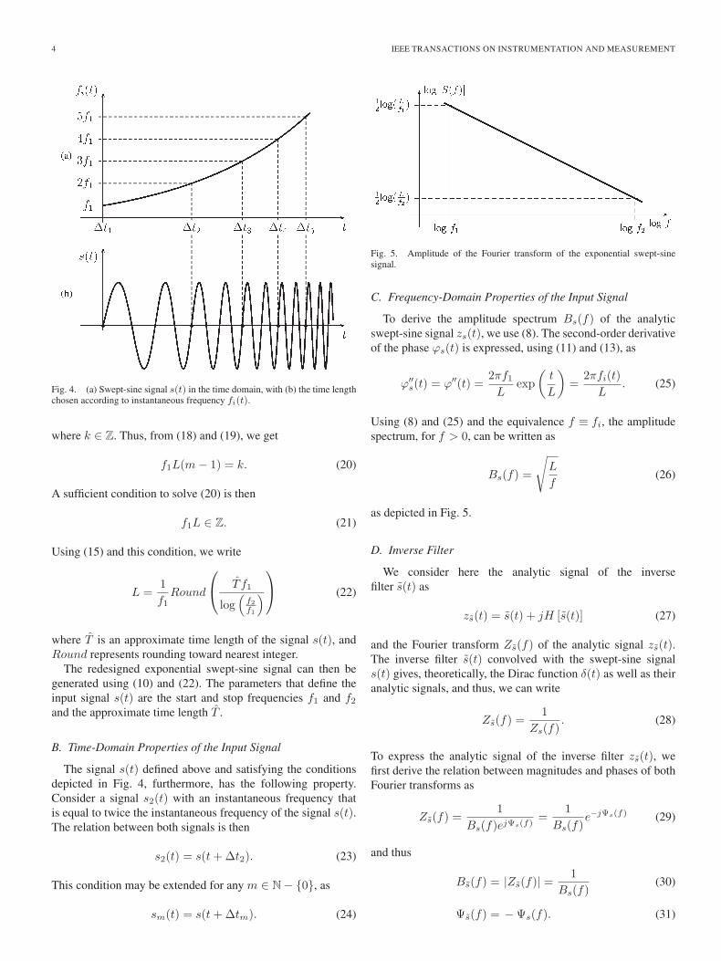
Second, as depicted in Fig. 4, the swept-sine signal s(t) at aparticular time lag Δtm is designed to be equal to zero, i.e.,s(Δtm) = 0, with the additional constraint of a positive firstderivative, i.e., s′(Δtm) > 0. These conditions consequentlyyield to

ϕ(Δtm) = 2kπ (19)


Fig. 4. (a) Swept-sine signal s(t) in the time domain, with (b) the time lengthchosen according to instantaneous frequency fi(t).

where k ∈ Z. Thus, from (18) and (19), we get

f1L(m − 1) = k. (20)

A sufficient condition to solve (20) is then

f1L ∈ Z. (21)

Using (15) and this condition, we write

L =1f1

Round

⎛⎝ T f1

log(

f2f1

)⎞⎠ (22)

where T is an approximate time length of the signal s(t), andRound represents rounding toward nearest integer.

The redesigned exponential swept-sine signal can then begenerated using (10) and (22). The parameters that define theinput signal s(t) are the start and stop frequencies f1 and f2

and the approximate time length T .

B. Time-Domain Properties of the Input Signal

The signal s(t) defined above and satisfying the conditionsdepicted in Fig. 4, furthermore, has the following property.Consider a signal s2(t) with an instantaneous frequency thatis equal to twice the instantaneous frequency of the signal s(t).The relation between both signals is then

s2(t) = s(t + Δt2). (23)

This condition may be extended for any m ∈ N − {0}, as

sm(t) = s(t + Δtm). (24)

Fig. 5. Amplitude of the Fourier transform of the exponential swept-sinesignal.

C. Frequency-Domain Properties of the Input Signal

To derive the amplitude spectrum Bs(f) of the analyticswept-sine signal zs(t), we use (8). The second-order derivativeof the phase ϕs(t) is expressed, using (11) and (13), as

ϕ′′s(t) = ϕ′′(t) =

2πf1

Lexp

(t

L

)=

2πfi(t)L

. (25)

Using (8) and (25) and the equivalence f ≡ fi, the amplitudespectrum, for f > 0, can be written as

Bs(f) =

√L

f(26)

as depicted in Fig. 5.

D. Inverse Filter

We consider here the analytic signal of the inversefilter s(t) as

zs(t) = s(t) + jH [s(t)] (27)

and the Fourier transform Zs(f) of the analytic signal zs(t).The inverse filter s(t) convolved with the swept-sine signals(t) gives, theoretically, the Dirac function δ(t) as well as theiranalytic signals, and thus, we can write

Zs(f) =1

Zs(f). (28)

To express the analytic signal of the inverse filter zs(t), wefirst derive the relation between magnitudes and phases of bothFourier transforms as

Zs(f) =1

Bs(f)ejΨs(f)=

1Bs(f)

e−jΨs(f) (29)

and thus

Bs(f) = |Zs(f)| =1

Bs(f)(30)

Ψs(f) = − Ψs(f). (31)


For asymptotic signal zs(t), the analytic inverse filter zs(t) is,consequently, also an asymptotic signal, i.e.,

zs(t) = as(t)ejϕs(t). (32)

Then, we derive the phase ϕs(t) from the expression of tf (f).Using (7) and (31), we get

tf (f) = − 12π

dΨs(f)df

=12π

dΨs(f)df

. (33)

Consequently, we get

tf (f) = − tf (f) (34)

ϕs(t) = ϕs(−t). (35)

We use (8) to derive the amplitude as(t) of the inverse filter asfollows:

Bs(f) =as(tf )√12π

∣∣ϕ′′s(tf )

∣∣ . (36)

As ϕ′′s(tf ) = ϕ′′

s(tf ) [from (34) and (35)], we can substitutefrom (25)

Bs(f) =as(tf )√

fL

. (37)

Now, from (26), (30), and (37) we can write

as(tf ) =fi

L. (38)

Using (12), the envelope as(t) is given by

as(t) =f1

Lexp

(− t

L

)(39)

and the analytic inverse filter is finally expressed as

zs(t) =f1

Lexp

(− t

L

)ej(ϕs(−t)) (40)

i.e., in shorten form, we have

zs(t) =f1

Lexp

(− t

L

)zs(−t). (41)

The inverse filter s(t) is then

s(t) =f1

Lexp

(− t

L

)s(−t). (42)

IV. PRINCIPLES OF THE METHOD OF IDENTIFICATION

In Section III, the input signal s(t) and the inverse filters(t) have been defined to be used for identification of the NLSunder test. This section focuses on the relation between partialfrequency responses Hm(f) and linear filters Gn(f) in thefrequency domain.

As the impulse responses hm(t) and gn(t), defined as theinverse Fourier transform of Hm(f) and Gn(f), respectively,

are supposed to be real functions, it follows from the Hermitianproperties of Hm(f) and Gn(f) that only the half frequencyarea f > 0 is considered in the following.

Given the partial frequency responses Hm(f) defined by (2),the frequency response of the linear filters Gn(f) of the powerseries nonlinear model can be derived analytically using thetrigonometric power formulas, defined as [22]

(sin x)2l+1 =(−1)l

4l

l∑k=0

(−1)k

(2l + 1

k

)sin [(2l + 1 − 2k)x]

(43)

∀ l ∈ N and

(sin x)2l =(−1)l

22l−1

l−1∑k=0

(−1)k

(2l

k

)cos [2(l − k)x] +

122l

(2l

l

)(44)

∀ l ∈ N − {0}.Regarding the Fourier transform of (43) and (44), and noting

FTp the result of the Fourier transform only for positive fre-quencies, we can write

FTp

{(sin x)2l+1

}=

(−1)l

4l

l∑k=0

(−1)k

(2l + 1

k

)

×FTp {sin [(2l + 1 − 2k)x]} (45)

∀ l ∈ N and

FTp

{(sin x)2l

}= j

(−1)l

22l−1

l−1∑k=0

(−1)k

(2l

k

)

×FTp {sin [2(l − k)x]} +1

22l

(2l

l

)(46)

∀ l ∈ N − {0}.These formulas give in the Fourier domain the relation

between the higher order harmonic sin(lx) and the lth power ofthe harmonic signal sinl(x), for l ∈ N. Considering a harmonicinput signal of frequency f0 > 0, the values of the frequencyresponses Hm(lf0) and the values of the frequency responsesof the linear filters Gn(lf0) are related in the same way as in(43) and (44).

The trigonometric formulas in the frequency domain can thenbe rewritten into the matrix form (47), where the matrices Aand B represent the coefficients in (45) and (46), i.e.,⎛

⎜⎜⎝FTp{sin x}FTp{sin2 x}FTp{sin3 x}

...

⎞⎟⎟⎠ = A

⎛⎜⎜⎝

FTp{sin x}FTp{sin 2x}FTp{sin 3x}

...

⎞⎟⎟⎠ + B. (47)

The matrix A is defined, according to (45) and (46), as

An,m =

⎧⎪⎨⎪⎩

(−1)2n+ 1−m2

2n−1

(n

n−m2

), for n ≥ m and

(n + m) is even0, else.

(48)

The matrix B is a one-column matrix and represents the con-stant values of the even power series. These values are only


Fig. 6. Simulated NLS with memory.

linked to the mean value of the output signal. The relationbetween the partial frequency response Hm(f0), for f0 > 0,and the linear filters Gn(f0) from the power series nonlinearmodel is given using the coefficients of the matrix A. Eachpartial frequency response Hm(f0), or mth harmonic, can beexpressed as a sum of the mth harmonics of all the nth powersweighted by the linear filters Gn(f0). The coefficients of themth harmonics of the nth power are A(n,m) and thus

Hm(f0) =N∑

n=1

An,mGn(f0). (49)

Finally, the linear transformation between Hm(f0) and Gn(f0),for f0 > 0, can generally be expressed in matrix form as⎛

⎜⎜⎝G1(f0)G2(f0)G3(f0)

...

⎞⎟⎟⎠ = (AT )−1

⎛⎜⎜⎝

H1(f0)H2(f0)H3(f0)

...

⎞⎟⎟⎠ (50)

where AT denotes the transpose of A.

V. RESULTS

A. Simulation of an NLS With Memory

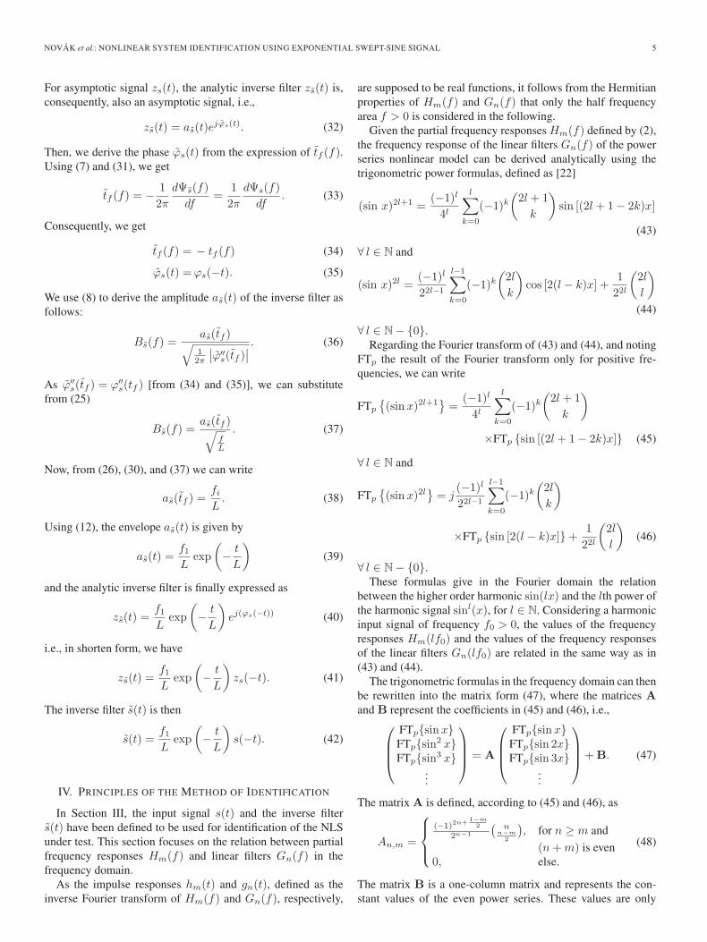
To illustrate the method, a simulated NLS with memory isidentified. This NLS consists of two nonlinear branches withlinear and cubic parts, each of them followed by a linear filter(Fig. 6). To simulate real-world conditions, a white Gaussiannoise n(t) is added to the output signal. Both filters are digitalButterworth filters. The filter G1(f) used in the linear branchis a tenth-order high-pass filter, with a cutoff frequency of500 Hz, and the filter G3(f) used in the cubic branch is atenth-order low-pass filter, with a cutoff frequency of 1 kHz.The simulation is performed using a sampling frequency fs =12 kHz. The excitation signal used for the identification is aswept-sine signal, as defined in Section III, with the followingparameters: f1 = 20 Hz; f2 = 2000 Hz; and T = 5 s. Themaximum frequency f2 has been chosen to avoid any aliasing[23], [24]. The order of the model is set to N = 3. Once theresponse of the NLS under test to this excitation signal isknown, the nonlinear convolution described in Section IV isperformed, and the linear filters of the nonlinear model areestimated.

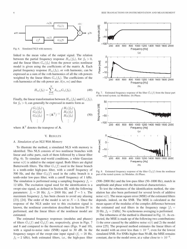
The estimated frequency responses (modulus and phases)of filters G1(f) and G2(f) are, respectively, given in Figs. 7and 8 and compared to the theoretical ones (Figs. 9 and 10),with a signal-to-noise ratio (SNR) equal to 30 dB. In thefrequency ranges of the swept-sine input signal (f1 = 20 Hz,f2 = 2 kHz), both estimated filters, i.e., the high-pass filter

Fig. 7. Estimated frequency response of the filter G1(f) from the linear partof the tested system. (a) Modulus. (b) Phase.

Fig. 8. Estimated frequency response of the filter G3(f) from the nonlinearpart of the tested system. (a) Modulus. (b) Phase.

(500–2000 Hz) and the low-pass filter (50–1000 Hz), match inamplitude and phase with the theoretical characteristics.

To test the robustness of the identification method, the sim-ulation has also been performed for several levels of additivenoise n(t). The mean square error (MSE) of the estimated filtersdepends, indeed, on the SNR. The MSE is calculated as themean square of the modulus of the complex difference betweenthe estimated and real filters in the frequency range [f1 =20 Hz, f2 = 2 kHz]. No synchronous averaging is performed.

The robustness of the method is illustrated in Fig. 11. As ex-pected, the MSE is made up of the following two contributions:1) the error caused by the additive noise n(t) and 2) the modelerror [25]. The proposed method estimates the linear filters ofthe model with an error less than 10−2, even for the lowestsimulated SNR. For SNRs higher than 50 dB, the MSE remainsconstant, due to the model error, at a value close to 10−6.


Fig. 9. Theoretical frequency response of the filter G1(f) from the linear partof the tested system. (a) Modulus. (b) Phase.

Fig. 10. Theoretical frequency response of the filter G3(f) from the nonlinearpart of the tested system. (a) Modulus. (b) Phase.

Fig. 11. Dependence of the MSE of the estimated filters G1(f) and G3(f)on SNR.

Fig. 12. Comparison of the real-world (thin) and regenerated (bold) responsesto the sine wave, with f = 500 Hz and A = 1 V. (a) Waveforms. (b) Spectra.

B. Identification of a Real NLS

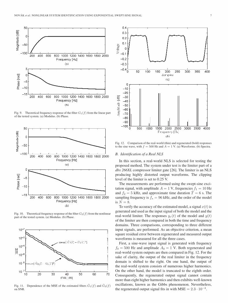
In this section, a real-world NLS is selected for testing theproposed method. The system under test is the limiter part of adbx 266XL compressor limiter gate [26]. The limiter is an NLSproducing highly distorted output waveforms. The clippinglevel of the limiter is set to 0.25 V.

The measurements are performed using the swept-sine exci-tation signal, with amplitude A = 1 V, frequencies f1 = 10 Hzand f2 = 5 kHz, and approximate time duration T = 6 s. Thesampling frequency is fs = 96 kHz, and the order of the modelis N = 8.

To verify the accuracy of the estimated model, a signal x(t) isgenerated and used as the input signal of both the model and thereal-world limiter. The responses yr(t) of the model and y(t)of the limiter are then compared in both the time and frequencydomains. Three comparisons, corresponding to three differentinput signals, are performed. As an objective criterion, a meansquare residual error between regenerated and measured outputwaveforms is measured for all the three cases.

First, a sine-wave input signal is generated with frequencyf0 = 500 Hz and amplitude A0 = 1 V. Both regenerated andreal-world system outputs are then compared in Fig. 12. For thesake of clarity, the output of the real limiter in the frequencydomain is shifted to the right. On one hand, the output ofthe real-world system consists of numerous higher harmonics.On the other hand, the model is truncated to the eighth order.Consequently, the regenerated output signal cannot containmore than eight higher harmonics and then exhibits well-knownoscillations, known as the Gibbs phenomenon. Nevertheless,the regenerated output signal fits in with MSE = 2.3 · 10−4.


Fig. 13. Comparison of the real-world (thin) and regenerated (bold) responsesto the sine wave, with f = 500 Hz and A = 0.3 V. (a) Waveforms. (b) Spectra.

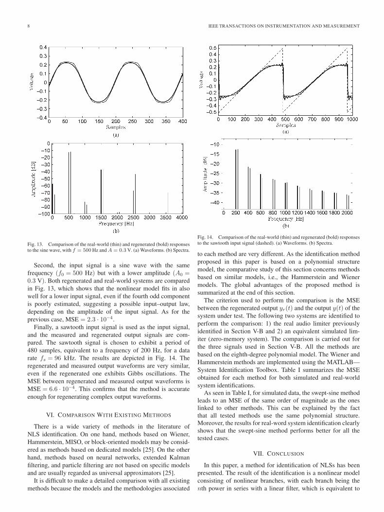
Second, the input signal is a sine wave with the samefrequency (f0 = 500 Hz) but with a lower amplitude (A0 =0.3 V). Both regenerated and real-world systems are comparedin Fig. 13, which shows that the nonlinear model fits in alsowell for a lower input signal, even if the fourth odd componentis poorly estimated, suggesting a possible input–output law,depending on the amplitude of the input signal. As for theprevious case, MSE = 2.3 · 10−4.

Finally, a sawtooth input signal is used as the input signal,and the measured and regenerated output signals are com-pared. The sawtooth signal is chosen to exhibit a period of480 samples, equivalent to a frequency of 200 Hz, for a datarate fs = 96 kHz. The results are depicted in Fig. 14. Theregenerated and measured output waveforms are very similar,even if the regenerated one exhibits Gibbs oscillations. TheMSE between regenerated and measured output waveforms isMSE = 6.6 · 10−4. This confirms that the method is accurateenough for regenerating complex output waveforms.

VI. COMPARISON WITH EXISTING METHODS

There is a wide variety of methods in the literature ofNLS identification. On one hand, methods based on Wiener,Hammerstein, MISO, or block-oriented models may be consid-ered as methods based on dedicated models [25]. On the otherhand, methods based on neural networks, extended Kalmanfiltering, and particle filtering are not based on specific modelsand are usually regarded as universal approximators [25].

It is difficult to make a detailed comparison with all existingmethods because the models and the methodologies associated

Fig. 14. Comparison of the real-world (thin) and regenerated (bold) responsesto the sawtooth input signal (dashed). (a) Waveforms. (b) Spectra.

to each method are very different. As the identification methodproposed in this paper is based on a polynomial structuremodel, the comparative study of this section concerns methodsbased on similar models, i.e., the Hammerstein and Wienermodels. The global advantages of the proposed method issummarized at the end of this section.

The criterion used to perform the comparison is the MSEbetween the regenerated output yr(t) and the output y(t) of thesystem under test. The following two systems are identified toperform the comparison: 1) the real audio limiter previouslyidentified in Section V-B and 2) an equivalent simulated lim-iter (zero-memory system). The comparison is carried out forthe three signals used in Section V-B. All the methods arebased on the eighth-degree polynomial model. The Wiener andHammerstein methods are implemented using the MATLAB—System Identification Toolbox. Table I summarizes the MSEobtained for each method for both simulated and real-worldsystem identifications.

As seen in Table I, for simulated data, the swept-sine methodleads to an MSE of the same order of magnitude as the oneslinked to other methods. This can be explained by the factthat all tested methods use the same polynomial structure.Moreover, the results for real-word system identification clearlyshows that the swept-sine method performs better for all thetested cases.

VII. CONCLUSION

In this paper, a method for identification of NLSs has beenpresented. The result of the identification is a nonlinear modelconsisting of nonlinear branches, with each branch being thenth power in series with a linear filter, which is equivalent to


TABLE IMSES

the generalized polynomial Hammerstein model. The methodallows in particular to regenerate an output signal correspond-ing to any given input signal and to compare this regeneratedoutput signal to the real-world output to validate the accuracyof the model.

The method has been applied to a real-world NLS (audiolimiter). The nonlinear model has been tested for different inputsignals, i.e., two sine-wave signals with different levels and asawtooth signal, and compared with other methods.

On one hand, one of the characteristics of the method isthe necessity of properly designed excitation signal. For thatreason, the system under test cannot be excited from a simplesignal generator, but from a personal computer with an audiocard, or from a signal generator with memory, in which theproperly designed signal is recorded.

On the other hand, the robustness of the method has beenproved regarding noise characteristics (Fig. 11) and througha real measurement test (Table I), as also presented in [16]and [17]. It has also worth noting that the method has a lowcalculation time cost. Compared to the methods that are notbased on a specific model (e.g., extended Kalman filtering,particle filtering, or neural networks), the proposed method isstraightforward with no special algorithms and, thus, easy tobe implemented. In addition, the method has no need for anyknowledge of the system under test.

REFERENCES

[1] T. Kailath, Linear Systems. Englewood Cliffs, NJ: Prentice-Hall, 1980.[2] B. P. Lathi, Signal Processing and Linear Systems. Oxford, U.K.:

Oxford Univ. Press, 2000.[3] M. Schetzen, The Volterra and Wiener Theories of Nonlinear Systems.

New York: Wiley, 1980.[4] O. Nelles, Nonlinear System Identification: From Classical Approaches to

Neural Networks and Fuzzy Models. Berlin, Germany: Springer-Verlag,2001.

[5] J. S. Bendat, Nonlinear System Techniques and Applications. New York:Wiley, 1998.

[6] F. Thouverez and L. Jezequel, “Identification of NARMAX models on amodal base,” J. Sound Vib., vol. 189, no. 2, pp. 193–213, Jan. 1996.

[7] H. E. Liao and W. S. Chen, “Determination of nonlinear delay ele-ments within NARMA models using dispersion functions,” IEEE Trans.Instrum. Meas., vol. 46, no. 4, pp. 868–872, Aug. 1997.

[8] Y.-W. Chen, S. Narieda, and K. Yamashita, “Blind nonlinear system iden-tification based on a constrained hybrid genetic algorithm,” IEEE Trans.Instrum. Meas., vol. 52, no. 3, pp. 898–902, Jun. 2003.

[9] H. Sorenson, Kalman Filtering: Theory and Application. Montvale, NJ:IEEE Press, 1985.

[10] O. Cappé, S. J. Godsill, and E. Moulines, “An overview of existing meth-ods and recent advances in sequential Monte Carlo,” Proc. IEEE, vol. 95,no. 5, pp. 899–924, May 2007.

[11] P. Crama and J. Schoukens, “Initial estimates of Wiener and Hammersteinsystems using multisine excitation,” IEEE Trans. Instrum. Meas., vol. 50,no. 6, pp. 1791–1795, Dec. 2001.

[12] M. Solomou, D. Rees, and N. Chiras, “Frequency domain analysis of non-linear systems driven by multiharmonic signals,” IEEE Trans. Instrum.Meas., vol. 53, no. 2, pp. 243–250, Apr. 2004.

[13] E. Ceri and D. Rees, “Nonlinear distortions and multisine signals—Part 1: Measuring the best linear approximation,” IEEE Trans. Instrum.Meas., vol. 49, no. 3, pp. 602–609, Jun. 2000.

[14] A. H. Tan and K. Godfrey, “The generation of binary and near-binarypseudorandom signals: An overview,” IEEE Trans. Instrum. Meas.,vol. 51, no. 4, pp. 583–588, Aug. 2002.

[15] R. Haber and L. Keviczky, Nonlinear System Identification: Input/OutputModeling Approach, vol. 1/2. Dordrecht, The Netherlands: Kluwer,1999.

[16] A. Farina, “Simultaneous measurement of impulse response and distortionwith a swept-sine technique,” in Proc. AES 108th Conv., Paris, France,Feb. 2000.

[17] E. Armelloni, A. Farina, and A. Bellini, “Non-linear convolution: A newapproach for the auralization of distorting systems,” in Proc. AES 110thConv., Amsterdam, The Netherlands, May 2001.

[18] L. Cohen, Time–Frequency Analysis. Englewood Cliffs, NJ: Prentice-Hall, 1995.

[19] P. Flandrin, Time–Frequency/Time-Scale Analysis. San Diego, CA:Academic, 1999.

[20] L. Cohen, “Instantaneous frequency and group delay of a filtered signal,”J. Franklin Inst., vol. 337, no. 4, pp. 329–346, Jul. 2000.

[21] T. Kite, “Measurement of audio equipment with log-swept sine chirps,”in Proc. AES 117th Conv., San Francisco, CA, Oct. 2004.

[22] W. H. Beyer, Standard Mathematical Tables. Boca Raton, FL: CRCPress, 1987.

[23] Y. M. Zhu, “Generalized sampling theorem,” IEEE Trans. Circuits Syst.II, Analog Digit. Signal Process., vol. 39, no. 8, pp. 587–588, Aug. 1992.

[24] J. Tsimbinos and K. V. Lever, “Input Nyquist sampling suffices to identifyand compensate nonlinear systems,” IEEE Trans. Signal Process., vol. 46,no. 10, pp. 2833–2837, Oct. 1998.

[25] J. Schoukens, R. Pintelon, and Y. Rolain, “Identification of nonlinear andlinear systems, similarities, differences, challenges,” in Proc. 14th IFACSymp. Syst. Identification, Newcastle, Australia, 2006, pp. 122–124.

[26] WWW page Dbx: Professional Products, dbx 266xl Compressor-Gate2007. [Online]. Available: http://www.dbxpro.com/266XL/266XL.php

[27] J. S. Bendat and A. G. Piersol, Engineering Applications of Correlationand Spectral Analysis. New York: Wiley, 1980.

[28] P. Welch, “The use of the fast Fourier transform for the estimation ofpower spectra,” IEEE Trans. Audio Electroacoust., vol. AU-15, no. 70,pp. 70–73, Jun. 1970.

Antonín Novák received the Master degree inengineering from the Czech Technical University,Prague, Czech Republic, in 2006. He is currentlywith the Faculty of Electrotechnical Engineering,Czech Technical University, and the Laboratoired’Acoustique de l’Université du Maine, UMR-CNRS 6613, Le Mans, France, working toward aPh.D. degree within the framework of the Frenchgovernment program, “Cotutelle de thèse.”

His research interests include analysis and mea-surement of nonlinear systems and digital signal

processing.

http://www.dbxpro.com/266XL/266XL.php

http://www.dbxpro.com/266XL/266XL.php


Laurent Simon (M’00) was born in France in 1965.He received the Ph.D. degree in acoustics from theUniversité du Maine, Le Mans, France, in 1994.

He is currently a Professor with the Labo-ratoire d’Acoustique de l’Université du Maine,UMR-CNRS 6613, Le Mans. His research interestsmainly concern signal processing for acoustics andvibrations, including nonlinear system identification,inverse problems for NDT, and spectral estimation ofmissing data.

František Kadlec was born in Czech Republic in1943. He received the B.S. degree in electrical en-gineering and the Ph.D. degree in acoustics from theCzech Technical University, Prague, Czech Repub-lic, in 1967 and 1975, respectively.

He is currently with the Multimedia TechnologyGroup, Radio Engineering Department, Faculty ofElectrotechnical Engineering, Czech Technical Uni-versity. His research interests include audio signalprocessing, analysis of audio systems with nonlin-earities, and sound signals compression and testing

from the psychoacoustic point of view.

Pierrick Lotton was born in France, in 1967. Hereceived the Ph.D. degree in acoustics from the Uni-versité du Maine, Le Mans, France, in 1994.

He is currently a CNRS Research Fellow withthe Laboratoire d’Acoustique de l’Université duMaine, UMR-CNRS 6613, Le Mans. His researchinterests include electroacoustic transducers andthermoacoustics.

Dr. Lotton is a member of the Audio EngineeringSociety and the French Acoustical Society.

Documents

Nonlinear System Identification Using Exponential Swept-Sine Signal