Nonstationarity in the ‘resting brain's’ modular architecture

Non-Stationarity in the ‘‘Resting Brain’s’’ ModularArchitectureDavid T. Jones1, Prashanthi Vemuri2, Matthew C. Murphy2, Jeffrey L. Gunter2, Matthew L. Senjem2,

Mary M. Machulda3, Scott A. Przybelski4, Brian E. Gregg2, Kejal Kantarci2, David S. Knopman1,

Bradley F. Boeve1, Ronald C. Petersen1, Clifford R. Jack Jr.2*

1 Department of Neurology, Mayo Clinic, Rochester, Minnesota, United States of America, 2 Department of Radiology, Mayo Clinic, Rochester, Minnesota, United States of

America, 3 Department of Psychiatry/Psychology, Mayo Clinic, Rochester, Minnesota, United States of America, 4 Department of Biomedical Statistic and Informatics, Mayo

Clinic, Rochester, Minnesota, United States of America

Abstract

Task-free functional magnetic resonance imaging (TF-fMRI) has great potential for advancing the understanding andtreatment of neurologic illness. However, as with all measures of neural activity, variability is a hallmark of intrinsicconnectivity networks (ICNs) identified by TF-fMRI. This variability has hampered efforts to define a robust metric ofconnectivity suitable as a biomarker for neurologic illness. We hypothesized that some of this variability rather thanrepresenting noise in the measurement process, is related to a fundamental feature of connectivity within ICNs, which istheir non-stationary nature. To test this hypothesis, we used a large (n = 892) population-based sample of older subjects toconstruct a well characterized atlas of 68 functional regions, which were categorized based on independent componentanalysis network of origin, anatomical locations, and a functional meta-analysis. These regions were then used to constructdynamic graphical representations of brain connectivity within a sliding time window for each subject. This allowed us todemonstrate the non-stationary nature of the brain’s modular organization and assign each region to a ‘‘meta-modular’’group. Using this grouping, we then compared dwell time in strong sub-network configurations of the default modenetwork (DMN) between 28 subjects with Alzheimer’s dementia and 56 cognitively normal elderly subjects matched 1:2 onage, gender, and education. We found that differences in connectivity we and others have previously observed inAlzheimer’s disease can be explained by differences in dwell time in DMN sub-network configurations, rather than steadystate connectivity magnitude. DMN dwell time in specific modular configurations may also underlie the TF-fMRI findingsthat have been described in mild cognitive impairment and cognitively normal subjects who are at risk for Alzheimer’sdementia.

Citation: Jones DT, Vemuri P, Murphy MC, Gunter JL, Senjem ML, et al. (2012) Non-Stationarity in the ‘‘Resting Brain’s’’ Modular Architecture. PLoS ONE 7(6):e39731. doi:10.1371/journal.pone.0039731

Editor: Yong He, Beijing Normal University, China

Received February 15, 2012; Accepted May 25, 2012; Published June 28, 2012

Copyright: � 2012 Jones et al. This is an open-access article distributed under the terms of the Creative Commons Attribution License, which permitsunrestricted use, distribution, and reproduction in any medium, provided the original author and source are credited.

Funding: This work was supported by The National Institute on Aging (R01AG11378, P50 AG16574, U01 AG06786, K99AG37573), the Alexander FamilyAlzheimer’s Disease Research Professorship of the Mayo Foundation, and Alzheimer’s Association New Investigator grant. The funders had no role in study design,data collection and analysis, decision to publish, or preparation of the manuscript.

Competing Interests: The authors have declared that no competing interests exist.

* E-mail: [email protected]

Introduction

Functional magnetic resonance imaging (fMRI) conducted

without a predetermined experimental condition (sometimes

referred to as resting-state fMRI), is emerging as a powerful tool

for investigating the intrinsic organization of large portions of the

brain into networks of synchronized activity [1]. Network informa-

tion is found by analyzing low-frequency oscillations (,0.1 Hz) in

the blood-oxygenation level dependent (BOLD) signal. These

oscillations are readily observed with MRI systems available at

most medical centers. The absence of an experimentally predeter-

mined task in these studies has led to the popularization of the term

resting-state fMRI to refer to the technique, and the term resting-

state networks to refer to the identified brain networks. However, the

networks identified using resting-state fMRI are also identified when

applying the same analysis techniques to task-based fMRI exper-

imental designs when the brain is not at ‘‘rest’’ [2]. Therefore, the

technique is more accurately referred to as task-free fMRI (TF-

fMRI), and the identified networks as intrinsic connectivity networks

(ICNs) [3]. Removing ‘‘rest’’ from these terms more accurately

captures the dynamic nature of the functional connectivity that

characterizes these large-scale networks [4], as the brain is never

truly at ‘‘rest.’’

Task-free fMRI has great potential for serving as a biomarker

for neurologic illness, however high variability in network

measures [5] may necessitate long scanning times to distinguish

an individual from the group [6]. We hypothesize that some of this

variability, rather than representing noise in the measurement

process [7], is related to a fundamental feature of connectivity

within ICNs, which is its non-stationary nature. Some of this

variability is undoubtedly related to the variability in brain states at

the time of the experimentally unconstrained scanning session.

Unconstrained brain activity is inherent in the TF-fMRI

experimental paradigm and this leads to variability in measures

of the organization of large-scale brain networks. This implies that

varying brain states will affect measures of network organization,

which has led some researchers to suggest restraining possible

PLoS ONE | www.plosone.org 1 June 2012 | Volume 7 | Issue 6 | e39731

brain states by administering a task [6]. However, introducing a

task reduces the appeal of the ease of TF-fMRI acquisition and

does not necessarily circumvent the need for understanding the

effects of the non-stationary nature of brain states on measures of

network connectivity.

The non-stationary nature of ICNs during an experimentally

unconstrained condition has been observed using magnetoen-

cephalography [8]. It has also recently been shown that ICNs are

related to shifting brain microstates measured via electroenceph-

alography (EEG) [9], which are characteristically non-stationary.

Yet, little is known about the variability in the organization of

ICNs over time in TF-fMRI data. However, a great deal has been

learned about the presumed stationary network properties of the

brain via application of graph theoretical analysis of TF-fMRI

data (see [10] for a review of complex network analysis

methodology).

Graph theoretical analyses have demonstrated that the network

architecture of the brain has scale-free small-world network

organization [11,12] and has a degenerate [13] hierarchically-

organized [14] modular architecture. The segregation of regions

within a graph into densely interconnected groups defines a

networks modular structure, and measures of this structure are

referred to as measures of modularity. The regions of the brain

comprising these modules have similarities across studies, and bear

resemblance to the most common networks identified as ICNs (e.g.

visual, motor, task-negative and task-positive regions [15]). Given

the non-stationarity in ICN, we hypothesize that the topographic

organization of the brain’s modular architecture also varies over

time, which may explain variability in the reported modular

assignments within separate datasets [16]. If this hypothesis is

validated, then the conceptualization of TF-fMRI modular

architecture as non-stationary would be consistent with a recent

report of the modular non-stationarity during task-based fMRI

[17], thus further linking observations of the organization of low-

frequency fluctuations during ‘‘rest’’ and task.

Understanding the dynamic network architecture in the human

brain is a prerequisite to understanding how neurological disease

alters this time-dependent topology. We have recently demon-

strated that the age-related changes in ICNs are similar to the

changes observed in Alzheimer’s disease (AD) [18], and other

investigators have shown that the modular organization of the

brain is also affected by aging [19]. Therefore, it is important to

study the normal modular architecture of the population at risk for

developing the neurologic illness of interest. The population based

sampling of healthy older subjects in the Mayo Clinic Study of

Aging (MCSA) [20] is ideally suited to define normal network

topology in the cognitively normal population at risk for common

neurodegenerative illnesses of the elderly, namely AD dementia.

For these same reasons it is important to atlas the brain

functionally [6] in this population as well.

This paper is organized into three major subsections. First, we

constructed a population-based functional atlas. This was done by

performing a large (N = 892) high dimensional independent

component analysis (ICA) decomposition of TF-fMRI data from

cognitively normal (CN) subjects drawn from the MCSA. This

ICA decomposition was used to atlas the brain into 68 functional

regions, which are categorized based on ICA network of origin,

anatomical locations, and a functional meta-analysis. Second, we

developed dynamic functional metrics to capture the non-

stationary nature of the brain’s network topography. This was

done by constructing dynamic graphical representations of brain

connectivity (between the atlas defined functional regions) using a

sliding time window correlation for each subject and then

characterizing these graphs using recently developed graph

metrics for modularity on fully connected and weighted networks

[13]. Lastly, we evaluated whether non-stationarity in this modular

organization was related to the reciprocal changes in connectivity

between the anterior default mode network (aDMN) and posterior

default mode network (pDMN) we have previously observed in

subjects with AD dementia [18].

Methods

SubjectsSubjects enrolled in the Mayo Clinic Study of Aging (MCSA), a

prospective, population based study of randomly selected residents

of Olmstead County, Minnesota, who had undergone TF-fMRI

and passed quality control (see below) at the time of this study were

included in this study (n = 892). The MCSA cohort is composed of

non-demented subjects age 70–90 plus and is balanced on gender.

Only cognitively normal (CN) MCSA subjects were used in this

first step in our analyses (Table 1). The details of MCSA subject

recruitment and design are detailed in a previous report [20]. In

summary, subjects undergo in-person evaluations by nurses,

physicians and neuropsychologists, during which they gathered

risk factor assessments including structured neurological exams

with mental status screening and routine neuropsychological

evaluation including tests measuring memory, language, executive

function and visuospatial skills. A final diagnosis for each subject is

made during a weekly consensus conference involving all study

faculty.

We also evaluated subjects with AD dementia (n = 28) in our

study. All met National Institute of Neurological Disorders and

Stroke and the Alzheimer’s Disease and Related Disorders

Association (NINDS-ADRDA) criteria and were participants of

the Mayo Clinic Alzheimer’s Disease Research Center.

Ethics StatementAll participants, or appropriate surrogates, provided written

informed consent for participation. The Mayo Clinic Institutional

Review Board approved the study and the consenting processes.

Task-Free fMRI Data Acquisition and PreprocessingTask-free fMRI data were acquired using a General Electric

3 T Signa HDx scanner, 8 channel head coil, gradient EPI,

TR = 3000 ms, TE = 30 ms, 90u flip angle, 21 cm field of view,

64664 in-plane matrix, slice thickness 3.3 mm without gap, and

103 or 113 volumes were obtained. Subjects were instructed to

keep their eyes open during scanning. All TF-fMRI data sets with

greater than 3 mm of translational movement, 3u of rotational

movement, or that failed visual inspection for obvious artifacts

were excluded from analysis (2.4% of studies did not pass these

quality control measures). Preprocessing and data analysis was

performed utilizing a combination of the Statistical Parametric

Mapping (SPM5) software (http://www.fil.ion.ucl.ac.uk/spm/

software/spm5/) (Wellcome Department of Cognitive Neurology,

University College London, UK), the Resting-State fMRI Data

Analysis Toolkit (REST) v1.5 (http://www.restfmri.net) [21], Data

Processing Assistant for Resting-State fMRI (DPARSF) v2.0

(http://www.restfmri.net) [22], group ICA of fMRI toolbox

(GIFT) software v2.0 c (http://icatb.sourceforge.net) [23], brain

connectivity toolbox (http://www.brain-connectivity-toolbox.net)

[10], and in-house developed software implemented in MATLAB

v7.11 (Mathworks Inc., Natick, MA, USA).

Preprocessing steps included discarding the first 3 volumes to

obtain steady state magnetization (sequences with 113 volumes

were also truncated so all sequences had 100 remaining volumes

for analysis), realignment, slice time correction, normalization to

Non-Stationarity in TF-fMRI


SPM5 EPI template, smoothing with 4 mm full-width half

maximum Gaussian kernel, linear detrending to correct for signal

drift, and 0.01–0.08 Hz bandpass filtering to reduce non-neuronal

contributions to BOLD fluctuations. In addition, regression

correction for spurious variables included rigid body transforma-

tion motion effects, global mean signal, white matter signal and

cerebral spinal fluid signal [24,25].

Construction of Population Based Atlas-using the TimeSeries of 892 CN Subjects

Independent component analysis. The first step for the

construction of the population based atlas was identification of

ICNs in the population. We used spatial group ICA method of

GIFT with both a low-dimensional estimation of 20 independent

components and a high-dimensional estimation of 54 components

to identify the ICNs in the population. The number of

components chosen for the high-dimensional ICA was based on

the components estimation procedure available in the GIFT

software package. To evaluate stability and obtain the centrotype

estimate of the independent components, both the high and low-

dimensional group ICA analyses were run with 100 iterations

using the ICASSO [26] function within the GIFT software

package (Figure 1). The aggregated group component maps were

scaled to Z values. Every component was visually inspected, and

similar networks in both high- and low-dimensional ICA were

identified to assist in naming the high-dimensional components

which were subsets of the lower dimensional components

(Figure 2). Artifactual components were visually identified during

this processes and discarded. Each high-dimensional independent

component was then assigned a name based on a combination of

ICA network of origin, anatomical locations, and the functional

meta-analysis result (see below). All further analyses are conducted

using the high-dimensional ICA components.

BrainMap functional meta-analysis. Next, we used the

BrainMap functional meta-analysis to aid us with the nomencla-

ture of the identified ICNs by associating each ICN with

behavioral domains. Using BrainMap’s behavioral metadata we

conducted a functional meta-analysis of the behavioral domains

which are overrepresented (relative to the entire brain) within a

10 mm cubic region of interest (ROI) centered at the Montreal

Neurologic Institute (MNI) coordinates corresponding to the peak

Z-score for each of the 31 ICNs identified by the high dimensional

ICA in a similar manner as outlined by Laird et al, 2009 [27].

BrainMap behavioral metadata is divided into broad domains

including; action, cognition, emotion, interoception, and sensation

(a complete list can be accessed at http://brainmap.org/scribe).

The action, cognition, and sensation domains have a significant

number of highly occurring sub-domains of interest, so these

categories were expanded for the subsequent analysis (a complete

list of these domains is listed on the top and bottom of Figure 3).

For each ICN ROI, a chi squared test was performed to

evaluate the proportion of each behavioral domains occurrence

within the ROI relative to the entire brain. In order to account for

the inherent multiple comparisons problem, a false discovery rate

(FDR) correction was utilized, and results are reported significant

at FDR corrected p,0.05 and p,0.01.

Development of Dynamic Functional Metrics-using theTime Series of 892 CN Subjects

Dynamic graph construction using sliding time

windows. All graph metrics used in this study were obtained

from the brain connectivity toolbox (http://www.brain-

connectivity-toolbox.net) [10]. In order to construct graphical

representations which retain interpretability in terms of the above

defined ICNs, the 31 ICNs identified by the high-dimensional ICA

were used to develop 68 ROIs to be used as graph nodes. The 68

nodes were created by applying a stringent threshold to the group

independent components defined by a Z-score greater than 7,

which resulted in distinct clusters within each of the components.

These clusters were then manually extracted using MRIcron

(http://www.mccauslandcenter.sc.edu/mricro/mricron/). Clus-

ters that crossed the midline were divided into right and left

ROIs. This resulted in the creation of 68 ROI images, which are

available for download at http://mayoresearch.mayo.edu/mayo/

research/jack_lab/supplement.cfm. The BOLD signal within

these 68 ROIs was then extracted from the pre-processed TF-

fMRI data across the 100 volumes for each subject. Pearson’s

correlation coefficient was then used to create the connectivity

matrices. With the recent development of graph metrics applicable

to fully connected and weighted graphs [13], it was not necessary

to restrict our graphical representations using only positive weights

and arbitrary r-value cutoffs.

With the aim of investigating the dynamic nature of the

brain’s modular structure, graphical representations were

constructed within the smallest odd numbered sliding time

window from which reliable modular graph metrics could be

obtained (an odd number time window allows for centering of

the obtained metric on one time point). To define the smallest

reliable window size, we used the variability within the recently

developed measure of goodness of modular partition metric, Q*

[13]. Graphs with high Q* have greater than chance-expected

total within module weight, and ranges from 0 to 1, and we

consider high Q* to be values above the Q* of the null model

of a randomized graph preserving the original graph’s degree-,

weight- and strength-distribution (see [13] for a complete

discussion of Q* and the null model). The variance in Q*

began to stabilize around a window size of 27 seconds (9

volumes) and dropped to 10% greater than the variance present

using half of the total volumes at a window length of 33 seconds

(11 volumes) (Figure 4). Therefore, all subsequent analyses were

Table 1. Cognitively normal cohort characteristics.

Study participantsn = 892

Study non-participantsn = 945

MCSA cognitively normal participantsn = 1837

No. of females (%) 438 (49) 472 (50) 910 (50)

Age, (q1, q3) 79 (75, 83) 81 (76, 85) 80 (76, 85)

Short Test of mental status (q1, q3){ 35 (33, 37) 34 (32, 36) 34 (33, 36)

The median (IQR) are reported for the continuous variables.{40 subjects missing the Short Test of mental status; 13 missing from the study participants and 27 from the study non-participants.doi:10.1371/journal.pone.0039731.t001



conducted using a window length of 33 seconds. At this window

length, 90 graphical representations of connectivity in each

individual brain could be created. This resulted in 80,280

graphs for 892 subjects which were used in the subsequent

modular analysis.

Modular analysis. For each of the 80,280 graphs, the

modular assignments and Q* was calculated. A degree-, weight-

and strength-distribution preserving null model was constructed

for each of the 80,280 graphs and the Q* was calculated for these

as well [13]. Comparisons between Q* and the null Q*

distribution was conducted using the Wilcoxon two-sided rank

sum test.

The number of modules each graph contained ranged from 2–5

modules at the predefined smallest reliable odd numbered window

length of 33 seconds. The proportion of each was calculated across

all graphs and the percent time, or modular dwell time, an

individual subject spent in the modular configurations was also

estimated (except for the 5 modular configuration given its

infrequent occurrence across the 80,280 graphs). In order to

examine the effect of window length on module number, the

modular proportion was also calculated across all possible window

lengths.

Next, we assigned each of the 68 ROIs to a single module,

allowing for subsequent graphical analysis. Given that the

Figure 1. Similarity between independent component estimates as a 2D CCA projection. The similarity between the independentcomponents identified in each of the 100 iterations of the group ICA for both the low-(A) and high-dimensional (B) runs. Points represent individualruns, grey convex hulls represent a cluster of the same independent component (labeled with component number), cyan circles represent the bestestimate of the independent component (centrotype), red shading indicates average intra-cluster similarity exceeds 0.9, and pink shading indicatesaverage intra-cluster similarity is between 0.8 and 0.9. If intra-cluster similarity is bellow 0.9, red lines are drawn between runs that have similaritygreater than 0.9. Compact clusters are indicative of high run-to-run similarity in the ICA solution for that component. 2D-two dimensional, CCA-curvilinear component analysis, ICA-independent component analysis.doi:10.1371/journal.pone.0039731.g001

Figure 2. Default mode sub-networks identified with the low- and high-dimensional independent component analysis of 892cognitively normal subjects. The DMN sub-networks identified with low- (top) and high-dimensional (bottom) ICA displayed at Z.7 overlaid onanatomical reference. The colored high-dimensional independent components were split from their low-dimensional counterpart displayed above;cyan-vDMN, green-adDMN, pink-avDMN, blue-pDMN, yellow-dDMN, red-tDMN. DMN-default mode network, ICA-independent component analysis,vDMN-ventral default mode network, adDMN-anterior dorsal default mode network, avDMN-anterior ventral default mode network, pDMN-posteriordefault mode network, dDMN-dorsal default mode network, tDMN-temporal default mode network.doi:10.1371/journal.pone.0039731.g002



modular assignment number is arbitrary and not necessarily

related from graph to graph (numbers denoting groups ranging

from 1–5) and the non-stationarity in modular composition, we

grouped together nodes that tended to get the same modular

assignment number across the different modular configurations

in order to define a ‘‘meta-modular’’ structure. For example,

visual system nodes may receive a modular assignment of

module label 1 within a 2 modular configuration, while other

nodes are then assigned module label 2. While in another 2

module configuration, the visual and auditory nodes are

Figure 3. BrainMap functional meta-analysis. The results of the BrainMap functional meta-analysis are displayed for each of the 31 ICNsidentified in the high-dimensional ICA in 892 cognitively normal subjects. The ICNs are grouped by final modular assignment identified on the left(the language network ICN was included in TIL for this grouping). MNI coordinates for the peak Z-score are listed in parenthesis after the ICNabbreviation (names for abbreviations can be found in Table 2). The behavioral domains are color coded by BrainMap domain of origin; red-action,orange-cognitive, green-emotion, black-interoception, blue-perception. Plus signs indicate overrepresented, and minus signs indicateunderrepresented, relative to the entire brain. (+, 2) FDR p,0.05 (++, 22) FDR p,0.01 ICN-intrinsic connectivity network, ICA-independentcomponent analysis, SSM-somatic sensory-motor, TIL-temporal/insular/limbic, TPN-task-positive network, TNN-task-negative network, VIS-visual, MNI-Montreal Neurologic Institute.doi:10.1371/journal.pone.0039731.g003



Table 2. Node matrix order, module assignments, names, and abbreviations.

Module Name Node # Name AbbreviationFinalAssignment

Clustering ofAssignments

SSM 1 Left Face Face_L 1 1

2 Right Face Face_R 1 1

3 Left Hand Hand_L 1 1

4 Right Hand Hand_R 1 1

5 Left Leg Leg_L 1 1

6 Right Leg Leg_R 1 1

7 Left Parietal Operculum PrOp_L 1 1

8 Right Parietal Operculum PrOp_R 1 1

9 Left Superior Parietal Lobule SPL_L 1 1

10 Right Superior Parietal Lobule SPL_R 1 1

11 Left Dorsal Visual Stream DVS_L 1 1

12 Right Dorsal Visual Stream DVS_R 1 1

AIL 13 Left Auditory Aud_L 2 2

14 Right Auditory Aud_R 2 2

15 Left Superior Temporal ST_L 2 2

16 Right Superior Temporal ST_R 2 2

17 Posterior Language Lang_P 2 2

18 Left Temporal Default Mode Network tDMN_L 2 2

19 Right Temporal Default Mode Network tDMN_R 2 2

20 Left Anterior Limbic Network ALN_L 2 2

21 Right Anterior Limbic Network ALN_R 2 2

22 Left Posterior Limbic Network PLN_L 2 2

23 Right Posterior Limbic Network PLN_R 2 2

24 Left Deep Gray DG_L 2 2

25 Right Deep Gray DG_R 2 2

26 Left Insula Ins_L 2 2

27 Right Insula Ins_R 2 2

TPN 28 Left Inferior Temporal IT_L 3 3

29 Anterior Language Lang_A 3 3

30 Anterior Right Working Memory rWM_A 3 3

31 Posterior Right Working Memory rWM_P 3 3

32 Posterior Left Working Memory lWM_P 3 4

33 Left Attention Att_L 3 3

34 Right Attention Att_R 3 3

35 Anterior Cingulate Region of Salience Network SN_ACC 3 3

36 Left Lateral Region of Salience Network SN_L_Lat 3 3

37 Right Lateral Region of Salience Network SN_R_Lat 3 3

38 Left Anterior Ventral Lateral Prefrontal Cortex avlPFC_L 3 3

39 Right Anterior Ventral Lateral Prefrontal Cortex avlPFC_R 3 3

40 Left Posterior Ventral Lateral Prefrontal Cortex pvlPFC_L 3 3

41 Right Posterior Ventral Lateral Prefrontal Cortex pvlPFC_R 3 3

TNN 42 Left Lateral Posterior Default Mode Network pDMN_L_Lat 4 3

43 Left Medial Posterior Default Mode Network pDMN_L_Med 4 4

44 Right Lateral Posterior Default Mode Network pDMN_R_Lat 4 3

45 Right Medial Posterior Default Mode Network pDMN_R_Med 4 4

46 Left Lateral Dorsal Default Mode Network dDMN_L_Lat 4 3

47 Left Medial Dorsal Default Mode Network dDMN_L_Med 4 4

48 Right Lateral Dorsal Default Mode Network dDMN_R_Lat 4 3

49 Right Medial Dorsal Default Mode Network dDMN_R_Med 4 4



assigned module label 2 while other nodes are assigned module

label 1. However, across all possible modular configurations, the

visual nodes were typically always assigned to the same module,

while other nodes’ co-assignment with the visual nodes was

more variable. Given this variability, we captured the ‘‘meta-

modular’’ configuration using Ward’s method of agglomerative

hierarchical clustering applied to the modular assignments for

all 80,280 graphs. Since the highest observed modular

configuration was 5, we report the meta-modular assignment

at a maximum cluster cutoff of 5. However, for the final

modular assignment we also considered the ICN of origin. For

visualization, the nodes were ordered within the connectivity

matrices based on this final modular group assignment.

Application to Alzheimer’s DiseaseWe applied the developed sliding time window graph

construction technique, using the 68 ROIs as nodes with final

modular assignments listed in Table 2, to a group of 28

Alzheimer’s disease patients to investigate if the non-stationary

nature of the brain’s network architecture is related to

differences observed in functional connectivity between AD

and CN subjects, see [28] for a recent review. Specifically, we

examined whether dwell time in a particular modular config-

uration is related to our previously reported differential effect of

Alzheimer’s disease on the aDMN and pDMN [18]. To this

end, we calculated the composite within-module degree Z-score

for each of the DMN sub-networks in the task-negative network

module (i.e. posterior, anterior, dorsal, and ventral DMN) using

the brain connectivity toolbox [10].The composite score was the

average score for each of the four nodes in the DMN sub-

network. DMN sub-networks were considered a strong contrib-

utor to the brain state if their composite within-module degree

Z-score was greater than the average (i.e. positive z-values). The

percentage of time in which the sub-network strongly contrib-

uted to an individual subject’s brain state is reported as the

DMN dwell time. The 28 AD subjects were matched 1:2 on

age, gender, and education to a subset of 56 CN subjects for

comparison. The pair-wise comparisons of DMN dwell time for

AD and CN subjects were conducted using the Wilcoxon two-

sided rank sum test.

Results

SubjectsGiven that one of the motivations for this study was to develop a

baseline for investigating Alzheimer’s disease and other neurode-

generative illnesses in the elderly population, a summary of the

sample characteristics of the subset of imaged CN patients used in

this study relative to the entire MCSA population are reported in

Table 1. The MCSA subjects with TF-fMRI were representative

to the subjects that were not included for analyses. The age-,

gender-, and education-matched subset of controls and AD

subjects’ demographics are reported in Table 3.

Population Based AtlasIndependent component analysis. The low-dimensional

ICA revealed 15 ICNs and the high-dimensional ICA revealed 31

ICNs. The low-dimensional ICA components tended to include

several of their higher-dimensional counterparts within the same

independent component. This information was retained when

naming the high-dimensional components. For example, the three

low-dimensional DMN components and the corresponding six

high-dimensional components which retain the DMN moniker are

shown in Figure 2. This splitting was characteristic of other

Table 2. Cont.

Module Name Node # Name AbbreviationFinalAssignment

Clustering ofAssignments

50 Left Lateral Ventral Default Mode Network vDMN_L_Lat 4 4

51 Left Medial Ventral Default Mode Network vDMN_L_Med 4 4

52 Right Lateral Ventral Default Mode Network vDMN_R_Lat 4 4

53 Right Medial Ventral Default Mode Network vDMN_R_Med 4 4

54 Left Anterior Dorsal Default Mode Network adDMN_L 4 4

55 Right Anterior Dorsal Default Mode Network adDMN_R 4 4

56 Left Anterior Ventral Default Mode Network avDMN_L 4 4

57 Right Anterior Ventral Default Mode Network avDMN_R 4 4

58 Left Cingulate Cing_L 4 4

59 Right Cingulate Cing_R 4 4

60 Supplementary Motor Area of Language Network Lang_SMA 4 4

VIS 61 Left Central Primary Visual cPV_L 5 5

62 Right Central Primary Visual cPV_R 5 5

63 Left Peripheral Primary Visual pPV_L 5 5

64 Right Peripheral Primary Visual pPV_R 5 5

65 Left Lingual Ling_L 5 5

66 Right Lingual Ling_R 5 5

67 Left Ventral Visual Stream VVS_L 5 5

68 Right Ventral Visual Stream VVS_R 5 5

SSM-somatic sensory-motor, TIL-temporal/insular/limbic, TPN-task-positive network, TNN-task-negative network, VIS-visual.doi:10.1371/journal.pone.0039731.t002



networks. The dorsal visual stream, ventral visual stream, and

primary visual network for peripheral vision were all in the same

low-dimensional independent component, while each had distinct

independent components in the high-dimensional ICA. While the

high-dimensional decomposition was finer grained, it was also

more susceptible to the stochastic nature of the group ICA

algorithm. This manifested in less compact clustering of the 100

repeated group ICA runs using the ICASSO procedure in the

high-dimensional ICA compared to the low-dimensional (Figure 1).

The MNI coordinates for the peak Z-score of each high-

dimensional ICN are included in Figure 3. The aggregate

component maps for both the high- and low- dimensional ICA

are available for download at http://mayoresearch.mayo.edu/

mayo/research/jack_lab/supplement.cfm.

BrainMap functional meta-analysis and network

nomenclature. The BrainMap functional meta-analysis re-

vealed a statistically significant result for 26 of the 31 ICNs

(Figure 3). This information was then used to better inform the

final network nomenclature. For example, the dorsal and ventral

visual stream networks, which are sometimes referred to as lateral

visual ICN, had a functional meta-analysis result consistent with

properties associated with the dorsal and ventral processing

pathways (i.e. the ventral stream was associated with the language

domain and the dorsal was associated with the spatial domain,

fitting with the ‘‘what’’ and ‘‘where’’ pathway distinction). The

functional meta-analysis also highlighted the distinct differences in

two ICNs which involved the primary visual cortex. One of these

networks was strongly associated with the vision domain in the

meta-analysis, while the other was below statistical significance in

the visual domain but was highly significant in its association with

the auditory domain. This suggests that the visual network strongly

associated with audition is likely representative of the portion of

the primary visual cortex dedicate to the peripheral visual field,

which is commonly observed to co-activate in auditory fMRI

paradigms [29]. The anatomical location of these two visual ICNs

is also consistent with one accounting for the central visual field

and the other with the peripheral. The final visual-related ICN did

not have a significant result in the meta-analysis, however it largely

followed the anatomical extent of the lingual gyrus and therefore

we retained that anatomic moniker in this analysis. This naming

Figure 4. Q* versus window length in 892 cognitively normal subjects. The mean (green line) and standard deviation (error bars) of Q* areplotted for all graphs at each window length (A). The standard deviation of Q* is plotted as the percentage greater than the standard deviationpresent at a window length using half of the available volumes (50 volumes) and reported as the relative Q* variance (B). In order to define theshortest possible reliable odd window length, a predefined cutoff of a relative Q* variance of 10% was selected and is identified with a red line in Bdemonstrating the chosen window length of 11 volumes (33 seconds).doi:10.1371/journal.pone.0039731.g004



procedure was also informed by the ICA network of origin as

outlined above.

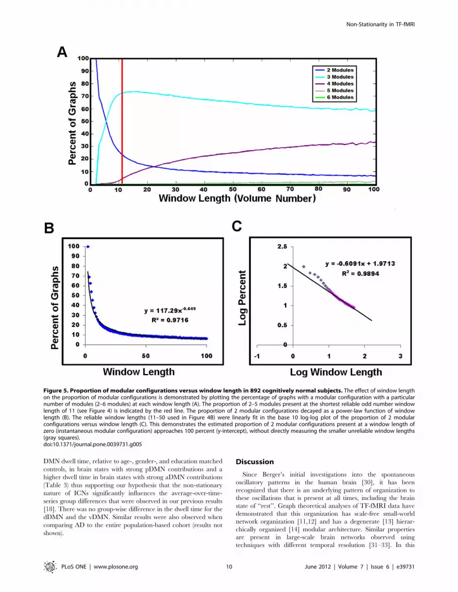
Modular AnalysisThe effect of window length on modular proportion is

significant, as would be expected in a non-stationary process

(Figure 5A). Longer window lengths measure predominately 3 and

4 modular configurations, consistent with a recent report on

several data sets analyzed at comparable window sizes [13]. The

proportion of 2 modular network configurations decreased as a

power-law function of window length (Figure 5B). Given that we

could not confidently decrease the window length beyond ,33

seconds (11 volumes), we attempted to estimate the instantaneous

(i.e. window length of zero) proportion of 2 module configurations.

To this end, we created a log-log plot of the proportion of 2

modular configurations versus the window lengths used in the

assessment of reliability (Figure 4B). We then linearly fit the

reliable window lengths (11–50 volumes) in the log-log plot and

calculated the y-intercept (Figure 5C). This revealed that the

estimated instantaneous proportion of 2 module configurations

approached 100% (actual estimate was 93.6%). In addition,

window lengths smaller than 11 in the log-log plot fall off the linear

trend of the more reliable window lengths further supporting our

use of the smallest possible reliable window length of 33 seconds

(11 volumes).

Each of the 80,280 graphs, form the shortest reliable odd

number window length of 33 seconds, displayed a highly modular

architecture relative to the null model (median and interquartile

range for Q* = 0.55, 0.52–0.59, and for null Q* = 0.16, 0.15–0.17,

p = 0). This result indicates that the high Q* values, characteristic

of dynamic brain connectivity matrices, are measuring true

modularity that is consistently greater than any potential chance

modular structure present in each of the 80,280 graphs.

The number of modules within each of the 80,280 graphs varied

between 2 and 5, at the predefined smallest reliable odd numbered

window length of 33 seconds (11 volumes), with 23.63% in a 2

module configuration, 72.38% in a 3 module configuration, 3.98%

in a 4 module configuration, and less than 0.01% in a 5 module

configuration (red line in Figure 5A). This distribution across all

graphs was similar for the modular dwell time within the 90 graphs

from a single subject’s scanning session, with each of the 892

subjects spending the majority of time during the scanning session

in a brain state with either a 2 or 3 module configuration at a

window length of 33 seconds (Figure 6).

The agglomerative hierarchical clustering of the modular

assignments into ‘‘meta-modular’’ groupings revealed clusters

largely composed of nodes from related ICNs (Figure 7). Even

though this was expected, it was further validation that nodes

within an ICN behaved synchronously in graphical form as

well. The ‘‘meta-modules’’ consisted of a somatic-sensory motor

module (SSM), temporal/insular/limbic module (TIL), task-

negative network module (TNN), task-positive network module

(TPN), and a visual module (VIS). While it is true that most

nodes clustered back with the ICN from which they were

derived, there were some exceptions. The lateral parietal

portions of the posterior DMN (pDMN) and dorsal DMN

(dDMN) clustered with the task-positive network. We elected,

however, to assign nodes derived from the same ICN to the

same module for the final modular assignment. An exception

was made for the language ICN because the three nodes in the

language ICN were all assigned to different clusters; the anterior

language node (left frontal operculum) to the TPN, the posterior

language node (left temporo-parietal) to the TIL, and the

supplementary motor area node to the TNN. The ‘‘meta-

modular’’ clustering and final nodal assignments are listed in

Table 2, and the spatial extents of the final 5 modular

assignments are displayed in Figure 8.

The average connectivity matrix for all 80,280 graphs

revealed that the VIS module had strong average within

module connectivity (Figure 9A). However, the dorsal visual

stream also had greater average connectivity with the VIS

module rather than the SSM module in which it was grouped

in the cluster analysis of modular assignment. Similar discrep-

ancies between modular clustering and the average connectivity

matrix are evident in other networks as well; however there

remains strong agreement between the average connectivity

matrix and the final modular assignment. Still, it is clear that

both the average connectivity matrix and final modular

assignments do not capture the non-stationary nature of the

brain’s modular architecture (Figure 9 B and C). The

connectivity between nodes varied continuously across the

scanning session (see Videos S1 and S2), which in turn leads

to varying graph topography which does not resemble the group

average. This was also true for the average connectivity matrix

for an individual subject, in which the average topography was

driven by the dwell time in particular modular configurations.

In other words, the longer a subject spent in a particular brain

state, the more it contributed to the topography of the average

connectivity matrix.

Application to Alzheimer’s DiseaseTo examine whether dwell time in a particular configuration is

related to our previously reported differential effect of Alzheimer’s

disease on the aDMN and pDMN [18], we calculated the

composite within-module degree Z-score for each of the DMN

sub-networks in the TNN module (i.e. posterior, anterior, dorsal,

and ventral DMN). We found that Alzheimer’s subjects had lower

Table 3. Comparison of DMN sub-network dwell timebetween Alzheimer’s and age-, gender-, and education-matched cognitive normal subjects.

CN (n = 56) AD (n = 28) p-value

No. of females (%) 20 (35.7) 10 (35.7) 1

Age (q1, q3) 78 (74, 84.5) 78 (74, 84.5) 0.92

Education (q1, q3) 15.5 (12,18) 15.5 (12,18) 0.97

STMS (q1, q3) 35 (33, 37) 23.5 (21.5, 29) ,0.001

CDR-SOB (q1, q3) 0.0 (0.0, 0.0) 4.5 (3.0, 6.8) ,0.001

pDMN DT (q1,q3) 52.8 (38.3, 63.9) 42.8 (21.7, 57.8) 0.048

aDMN DT (q1,q3) 57.8 (33.3, 75.6) 73.9 (58.9, 87.8) ,0.001

vDMN DT (q1,q3) 83.9 (68.9, 91.1) 80.0 (66.7, 87.8) 0.48

dDMN DT (q1,q3) 46.1 (29.4, 65.6) 39.4 (23.9, 56.7) 0.39

The median, IQR, and p-values from the Wilcoxon two-sided rank sum test arereported for the age, education, STMS, CDR-SOB, and dwell time in strong DMNsub-network modular configurations for AD subjects and age-, gender-, andeducation-matched CN subjects (the gender proportions and the p-value of thechi-squared test between groups is reported as well). DMN dwell time isdefined as the proportion of time (reported as a percentage) that a subjectspends in a particular modular configuration (strong DMN sub-networkconfigurations in this case) during the TF-fMRI scanning session.AD-Alzheimer’s disease, STMS-short test of mental status, CDR-SOB-clinicaldementia rating scale sum of boxes, aDMN-anterior default mode network, DT-dwell time, pDMN-posterior default mode network, vDMN-ventral default modenetwork, dDMN-dorsal default mode network, CN-cognitively normal, IQR-interquartile range, TF-fMRI-task-free functional magnetic resonance imaging.doi:10.1371/journal.pone.0039731.t003



DMN dwell time, relative to age-, gender-, and education matched

controls, in brain states with strong pDMN contributions and a

higher dwell time in brain states with strong aDMN contributions

(Table 3) thus supporting our hypothesis that the non-stationary

nature of ICNs significantly influences the average-over-time-

series group differences that were observed in our previous results

[18]. There was no group-wise difference in the dwell time for the

dDMN and the vDMN. Similar results were also observed when

comparing AD to the entire population-based cohort (results not

shown).

Discussion

Since Berger’s initial investigations into the spontaneous

oscillatory patterns in the human brain [30], it has been

recognized that there is an underlying pattern of organization to

these oscillations that is present at all times, including the brain

state of ‘‘rest’’. Graph theoretical analyses of TF-fMRI data have

demonstrated that this organization has scale-free small-world

network organization [11,12] and has a degenerate [13] hierar-

chically organized [14] modular architecture. Similar properties

are present in large-scale brain networks observed using

techniques with different temporal resolution [31–33]. In this

Figure 5. Proportion of modular configurations versus window length in 892 cognitively normal subjects. The effect of window lengthon the proportion of modular configurations is demonstrated by plotting the percentage of graphs with a modular configuration with a particularnumber of modules (2–6 modules) at each window length (A). The proportion of 2–5 modules present at the shortest reliable odd number windowlength of 11 (see Figure 4) is indicated by the red line. The proportion of 2 modular configurations decayed as a power-law function of windowlength (B). The reliable window lengths (11–50 used in Figure 4B) were linearly fit in the base 10 log-log plot of the proportion of 2 modularconfigurations versus window length (C). This demonstrates the estimated proportion of 2 modular configurations present at a window length ofzero (instantaneous modular configuration) approaches 100 percent (y-intercept), without directly measuring the smaller unreliable window lengths(gray squares).doi:10.1371/journal.pone.0039731.g005



study, we demonstrate that non-stationarity in the brain’s network

topography also exists at the temporal resolution of TF-fMRI

studies, and estimate that the instantaneous large-scale organiza-

tion of the brain is a binary modular state. This notion has face

validity because it implies that at any instant, the brain organizes

itself into an ‘‘active’’ module that is focused on a specific

functional quality, with portions of the reminder of the brain in a

‘‘non-active’’ state. We explored the composition of the varying

topography within the context of a well characterized functional

parcellation of the brain from a large population based sample of

subject’s at risk for AD dementia. This allowed us to demonstrate

that the non-stationary nature of the brains modular organization

is related to the differences in aDMN and pDMN connectivity in

AD dementia. However, even the non-stationary metric intro-

duced here remains burdened with high variability.

Figure 6. Histograms of modular dwell time in 2, 3, and 4 modular configurations at the smallest odd number reliable windowlength for the 892 cognitively normal subjects. The modular dwell time is defined as the proportion of time (reported as a percentage on the x-axis) that a subject spends in a modular configuration with a particular number of modules (i.e. 2,3, or 4) during the TF-fMRI scanning session.doi:10.1371/journal.pone.0039731.g006

Figure 7. Clustering of modular assignment for the 68 regions of interest, from the 892 cognitively normal subjects. The dendrogramfor the clustering of the 68 ROIs is displayed above. The colored regions in the dendrogram correspond to the similarly colored overlaid ROIs below(see Table 2 for each ROIs cluster assignment). ROI-region of interest.doi:10.1371/journal.pone.0039731.g007



Variability is a hallmark feature of measures of neural activity,

prompting the development of techniques which average across

multiple trials and subjects, or prolonging signal acquisition in

order to reduce this variability. These techniques as applied to TF-

fMRI have yet to yield a metric that is robust enough to be used as

a biomarker at the individual subject level [34]. Therefore, a better

understanding of the origins of the variability present in ICNs is

needed. Demographics such as age and gender are sources of

variability [35] as is the unconstrained nature of the task-free

experimental paradigm. However, only a small reduction in

variability related to the task-free experimental design is achieved

with the addition of a simple task [6], and highly structured tasks

Figure 8. Spatial extents of the 68 ROIs divided by final module assignment, from the 892 cognitively normal subjects. The spatialextents of the 68 ROIs are overlaid on a template brain using MRIcron. The network abbreviations are color-coded in the bottom right of each panel(see Table 2 for a list of corresponding names). The module abbreviations are listed to the left of each panel. ROI-region of interest, SSM-somaticsensory-motor, TIL-temporal/insular/limbic, TPN-task-positive network, TNN-task-negative network, VIS-visual.doi:10.1371/journal.pone.0039731.g008



typical of fMRI activation experiments still have a significant

amount variability necessitating averaging across trials and

subjects [36]. In addition, genetic factors such as APOE e4 carrier

status are also sources of variability independent of gray matter

density [37] and Alzheimer’s pathology [38]. However, controlling

for all of these factors will not circumvent the need for

understanding the effects of the non-stationary nature of brain

states on measures of network connectivity. It may indeed be the

case that the variability related to the non-stationary properties of

ICNs are the salient features which may distinguish AD-related

alterations of connectivity.

The inherent variability in large-scale neural networks was

more apparent in our high-dimensional ICA, as this analysis was

more susceptible to the stochastic nature of the ICA process

(Figure 1). The higher dimensional ICA was a finer-grained

parcellation of the brain across all of the subjects’ average

network configurations. This finer-grained solution may be the

reason for the greater variability, given that we observed that the

brain is organized into binary modular networks at any

instantaneous point in time, with finer-grained higher-order

modular configurations being observed by averaging binary states

over time. The regions of the brain within any given modular

organization were highly variable, but regions typically reported

as ICNs seemed to form common groupings within this varying

modular structure more often than not (Figure 8). This suggests

that the typically observed ICN (with accompanied anticorrela-

tions) represent an average representation of the most common

binary brain configurations over the observed time period. The

fact that at any given time the brain’s network topography

consists of a binary modular structure, may relate to the

difficulties human beings encounter while multitasking [39].

However, it should be noted that the relationship between the

large-scale organization of the brain’s connectivity and cognitive

performance remains uncertain. Although, our results (Figure 3)

and others [2,27,40] indicate that ICNs observed under the task-

free condition relate to observed results in highly structured task-

based fMRI studies. Developing a conceptual link between TF-

fMRI studies, task-based fMRI studies, and cognitive perfor-

mance will improve communication of results and allow for a

better understanding of the effect of neurologic disorders, such as

AD, on cognition and neural networks. To this end, non-

stationarity in modular composition should be considered an

intrinsic property of the brain’s organization in a ‘‘task-free’’ state

as well as ‘‘task-related’’ states [17].

The observed divergent changes between the aDMN and

pDMN, which we previously reported using ICA and seed-based

connectivity studies [18], are also present in the dwell time in

strong aDMN and pDMN brain states (Table 3). Compared to

CN, AD subjects had greater dwell time in strong aDMN sub-

network modular configurations and less dwell time in strong

pDMN configurations. Thus varying DMN dwell time in specific

modular configurations, rather than steady state connectivity

magnitude, seems to underlie the functional connectivity findings

that have been routinely described in AD dementia. Dwell time in

specific modular configurations may also underlie the TF-fMRI

findings that have been described in mild cognitive impairment

[41–44] and cognitively normal subjects who are at risk for AD

dementia [37,38,45,46]. It remains to be seen whether AD

associated changes in non-stationary connectivity metrics are

related to AD subjects transitioning into abnormal brain states, the

manner in which they transition between normal brain states, or a

combination of both. Future investigations into the reciprocal

pattern observed in pDMN and aDMN dwell time may also help

to clarify the mechanisms behind reciprocal network changes

commonly observed in TF-fMRI studies [47].

While this study has observed some of the properties of the non-

stationary nature of ICNs, it is yet to be shown how many

configurations are possible and what the composition of those

Figure 9. Fully connected and weighted graphs in 892 cognitively normal subjects. The fully connected and weighted graphicalrepresentation of the connectivity between the 68 ROIs at the smallest reliable odd number window length is displayed as connectivity matrices forthe average of all graphs (A) and two subjects (B and C). The color bar encodes Pearson correlation strength for all 3 figure panels. The 68 ROIs arearranged by final modular assignment (see Table 2 for ROI order). The within-module connections are highlighted with color-coded boxes for eachmodule in the average connectivity matrix (A). B and C display the average matrix for individual subjects (upper left corner inset of each panel) andevery tenth frame of the sliding time window analysis follows, which increase in time from left-to-right along the top row followed by the bottomrow. The videos of the entire sliding time window analysis for these two subjects are included in the supplementary material. SSM-somatic sensory-motor, TIL-temporal/insular/limbic, TPN-task-positive network, TNN-task-negative network, VIS-visual.doi:10.1371/journal.pone.0039731.g009



configurations might be. In this regard, future studies utilizing

instantaneous frequency estimates in graph construction may be

informative. This will be an important step to be taken in order to

better understand how neurodegenerative illnesses affect the

varying organization of the brain. In this regard, our study is

partially limited by the inherent heuristics present in our analysis

methodology; however the large sample size and null model gives

confidence that the properties reported here are robust. We do not

believe that the non-stationary nature of the brain’s complex

network architecture measured with TF-fMRI can be explained

simply by noise. Several features of the non-stationarity observed

in this study, beyond the difference identified in AD, support a

physiologically meaningful etiology.

Not only does modular dwell time vary within subjects across

the scanning session, but the nodal assignment to these modules

was highly variable. However, as can be readily appreciated from

Video S1 and S2, the variation was regular with multiple nodes

reorganizing the entire network by losing edges with one module

and gaining edges with another community simultaneously. We

attempted to capture some features of this dynamical process with

the agglomerative hierarchical clustering analysis (Figure 7). While

noise may seem like a plausible explanation for apparent non-

stationarity in a node-to-node correlation, the coordinated non-

stationarity present in the entire set of nodes, and the graphical

metrics characterizing the global network they comprise, can not

easily be attributable to noise alone. A more natural interpretation

would be that the scale-free nature of the brain’s network

architecture also extends to the property of non-stationarity

commonly observed at higher frequencies with more direct

electrophysiologic measures [8]. We hypothesize that the meta-

stable brain states observed in this analysis are the low-frequency

analogs of the higher-frequency microstates [9], albeit with

different temporal and spatial characteristics. More work is needed

to characterize these brain state configurations in their most

rudimentary binary form and how they associate over time to form

the higher-order network topography typically observed by

averaging over long window lengths. We intend for the high-

and low-dimensional decomposition of the MCSA TF-fMRI

cohort and the regions of interest used for non-stationary graph

construction to serve as a reference for ongoing investigations into

these properties (available for download at http://mayoresearch.

mayo.edu/mayo/research/jack_lab/supplement.cfm).

Supporting Information

Video S1 Entire sliding time window connectivitymatrix for the subject in Figure 9B in the main text.This supplementary video contains the complete sliding time

window analyses for the subject displayed in Figure 7B. The color

bar encodes Pearson correlation strength. The 68 ROIs are

arranged by final modular assignment (see Table 2 for ROI order).

The video plays at a rate of 3 frames per second with each frame

representing 3 seconds, which correspond to a playback rate 9

times faster than real time.

(ZIP)

Video S2 Entire sliding time window connectivitymatrix for the subject in Figure 9C in the main text.This supplementary video contains the complete sliding time

window analyses for the subject displayed in Figure 9C. The color

bar encodes Pearson correlation strength. The 68 ROIs are

arranged by final modular assignment (see Table 2 for ROI order).

The video plays at a rate of 3 frames per second with each frame

representing 3 seconds, which correspond to a playback rate 9

times faster than real time.

(ZIP)

Author Contributions

Conceived and designed the experiments: DTJ CRJ. Performed the

experiments: DTJ PV MCM. Analyzed the data: DTJ SAP BEG.

Contributed reagents/materials/analysis tools: DTJ MCM JLG MLS.

Wrote the paper: DTJ. Acquired data and obtained funding: DSK BFB

RCP CRJ. Performed clinical assessment: DSK BFB RCP. Interpreted

results: DTJ PV MCM JLG MLS MMM KK DSK BFB RCP CRJ.

Critically reviewed manuscript: DTJ PV MCM JLG MLS MMM SAP

BEG KK DSK BFB RCP CRJ.

References

1. Fox MD, Raichle ME (2007) Spontaneous fluctuations in brain activity observed

with functional magnetic resonance imaging. Nat Rev Neurosci 8: 700–711.

2. Smith SM, Fox PT, Miller KL, Glahn DC, Fox PM, et al. (2009)

Correspondence of the brain’s functional architecture during activation and

rest. Proc Natl Acad Sci U S A 106: 13040–13045.

3. Seeley WW, Menon V, Schatzberg AF, Keller J, Glover GH, et al. (2007)

Dissociable intrinsic connectivity networks for salience processing and executive

control. J Neurosci 27: 2349–2356.

4. Chang C, Glover GH (2010) Time-frequency dynamics of resting-state brain

connectivity measured with fMRI. Neuroimage 50: 81–98.

5. Wang JH, Zuo XN, Gohel S, Milham MP, Biswal BB, et al. (2011) Graph

theoretical analysis of functional brain networks: test-retest evaluation on short-

and long-term resting-state functional MRI data. PLoS One 6: e21976.

6. Anderson JS, Ferguson MA, Lopez-Larson M, Yurgelun-Todd D (2011)

Reproducibility of single-subject functional connectivity measurements. AJNR

Am J Neuroradiol 32: 548–555.

7. Maxim V, Sendur L, Fadili J, Suckling J, Gould R, et al. (2005) Fractional

Gaussian noise, functional MRI and Alzheimer’s disease. Neuroimage 25: 141–

158.

8. de Pasquale F, Della Penna S, Snyder AZ, Lewis C, Mantini D, et al. (2010)

Temporal dynamics of spontaneous MEG activity in brain networks. Proc Natl

Acad Sci U S A 107: 6040–6045.

9. Britz J, Van De Ville D, Michel CM (2010) BOLD correlates of EEG

topography reveal rapid resting-state network dynamics. Neuroimage 52: 1162–

1170.

10. Rubinov M, Sporns O (2010) Complex network measures of brain connectivity:

uses and interpretations. Neuroimage 52: 1059–1069.

11. van den Heuvel MP, Stam CJ, Boersma M, Hulshoff Pol HE (2008) Small-world

and scale-free organization of voxel-based resting-state functional connectivity in

the human brain. Neuroimage 43: 528–539.

12. Salvador R, Suckling J, Coleman MR, Pickard JD, Menon D, et al. (2005)

Neurophysiological architecture of functional magnetic resonance images of

human brain. Cereb Cortex 15: 1332–1342.

13. Rubinov M, Sporns O (2011) Weight-conserving characterization of complex

functional brain networks. Neuroimage 56: 2068–2079.

14. Meunier D, Lambiotte R, Fornito A, Ersche KD, Bullmore ET (2009)

Hierarchical modularity in human brain functional networks. Front Neuroin-

form 3: 37.

15. Fox MD, Snyder AZ, Vincent JL, Corbetta M, Van Essen DC, et al. (2005) The

human brain is intrinsically organized into dynamic, anticorrelated functional

networks. Proc Natl Acad Sci U S A 102: 9673–9678.

16. He Y, Wang J, Wang L, Chen ZJ, Yan C, et al. (2009) Uncovering intrinsic

modular organization of spontaneous brain activity in humans. PLoS One 4:

e5226.

17. Bassett DS, Wymbs NF, Porter MA, Mucha PJ, Carlson JM, et al. (2011)

Dynamic reconfiguration of human brain networks during learning. Proceedings

of the National Academy of Sciences of the United States of America 108: 7641–

7646.

18. Jones DT, Machulda MM, Vemuri P, McDade EM, Zeng G, et al. (2011) Age-

related changes in the default mode network are more advanced in Alzheimer

disease. Neurology 77: 1524–1531.

19. Meunier D, Achard S, Morcom A, Bullmore E (2009) Age-related changes in

modular organization of human brain functional networks. Neuroimage 44:

715–723.

20. Roberts RO, Geda YE, Knopman DS, Cha RH, Pankratz VS, et al. (2008) The

Mayo Clinic Study of Aging: design and sampling, participation, baseline

measures and sample characteristics. Neuroepidemiology 30: 58–69.

21. Song XW, Dong ZY, Long XY, Li SF, Zuo XN, et al. (2011) REST: a toolkit for

resting-state functional magnetic resonance imaging data processing. PLoS One

6: e25031.



22. Chao-Gan Y, Yu-Feng Z (2010) DPARSF: A MATLAB Toolbox for ‘‘Pipeline’’

Data Analysis of Resting-State fMRI. Front Syst Neurosci 4: 13.

23. Calhoun VD, Adali T, Pearlson GD, Pekar JJ (2001) A method for making

group inferences from functional MRI data using independent component

analysis. Hum Brain Mapp 14: 140–151.

24. Fox MD, Zhang D, Snyder AZ, Raichle ME (2009) The global signal and

observed anticorrelated resting state brain networks. J Neurophysiol 101: 3270–

3283.

25. Weissenbacher A, Kasess C, Gerstl F, Lanzenberger R, Moser E, et al. (2009)

Correlations and anticorrelations in resting-state functional connectivity MRI: a

quantitative comparison of preprocessing strategies. Neuroimage 47: 1408–

1416.

26. Himberg J, Hyvarinen A, Esposito F (2004) Validating the independent

components of neuroimaging time series via clustering and visualization.

Neuroimage 22: 1214–1222.

27. Laird AR, Eickhoff SB, Li K, Robin DA, Glahn DC, et al. (2009) Investigating

the functional heterogeneity of the default mode network using coordinate-based

meta-analytic modeling. J Neurosci 29: 14496–14505.

28. Vemuri P, Jones DT, Jack CR Jr (2012) Resting state functional MRI in

Alzheimer’s Disease. Alzheimers Res Ther 4: 2.

29. Cate AD, Herron TJ, Yund EW, Stecker GC, Rinne T, et al. (2009) Auditory

attention activates peripheral visual cortex. PLoS One 4: e4645.

30. Gloor P (1994) Berger lecture. Is Berger’s dream coming true? Electroencepha-

logr Clin Neurophysiol 90: 253–266.

31. Stam CJ (2004) Functional connectivity patterns of human magnetoencephalo-

graphic recordings: a ‘small-world’ network? Neurosci Lett 355: 25–28.

32. Van de Ville D, Britz J, Michel CM (2010) EEG microstate sequences in healthy

humans at rest reveal scale-free dynamics. Proc Natl Acad Sci U S A 107:

18179–18184.

33. Bassett DS, Meyer-Lindenberg A, Achard S, Duke T, Bullmore E (2006)

Adaptive reconfiguration of fractal small-world human brain functional

networks. Proc Natl Acad Sci U S A 103: 19518–19523.

34. Seibert TM, Majid DS, Aron AR, Corey-Bloom J, Brewer JB (2012) Stability of

resting fMRI interregional correlations analyzed in subject-native space: A one-

year longitudinal study in healthy adults and premanifest Huntington’s disease.

Neuroimage 59: 2452–2463.

35. Biswal BB, Mennes M, Zuo XN, Gohel S, Kelly C, et al. (2010) Toward

discovery science of human brain function. Proc Natl Acad Sci U S A 107:4734–4739.

36. McGonigle DJ, Howseman AM, Athwal BS, Friston KJ, Frackowiak RS, et al.

(2000) Variability in fMRI: an examination of intersession differences. Neuro-image 11: 708–734.

37. Machulda MM, Jones DT, Vemuri P, McDade E, Avula R, et al. (2011) Effectof APOE epsilon4 status on intrinsic network connectivity in cognitively normal

elderly subjects. Arch Neurol 68: 1131–1136.

38. Sheline YI, Morris JC, Snyder AZ, Price JL, Yan Z, et al. (2010) APOE4 AlleleDisrupts Resting State fMRI Connectivity in the Absence of Amyloid Plaques or

Decreased CSF A{beta}42. J Neurosci 30: 17035–17040.39. Marois R, Ivanoff J (2005) Capacity limits of information processing in the brain.

Trends Cogn Sci 9: 296–305.40. Laird AR, Fox PM, Eickhoff SB, Turner JA, Ray KL, et al. (2011) Behavioral

interpretations of intrinsic connectivity networks. J Cogn Neurosci 23: 4022–

4037.41. Li SJ, Li Z, Wu G, Zhang MJ, Franczak M, et al. (2002) Alzheimer Disease:

evaluation of a functional MR imaging index as a marker. Radiology 225: 253–259.

42. Bai F, Watson DR, Yu H, Shi Y, Yuan Y, et al. (2009) Abnormal resting-state

functional connectivity of posterior cingulate cortex in amnestic type mildcognitive impairment. Brain Res 1302: 167–174.

43. Sorg C, Riedl V, Muhlau M, Calhoun VD, Eichele T, et al. (2007) Selectivechanges of resting-state networks in individuals at risk for Alzheimer’s disease.

Proc Natl Acad Sci U S A 104: 18760–18765.44. Wang Z, Yan C, Zhao C, Qi Z, Zhou W, et al. (2011) Spatial patterns of

intrinsic brain activity in mild cognitive impairment and Alzheimer’s disease: a

resting-state functional MRI study. Hum Brain Mapp 32: 1720–1740.45. Hedden T, Van Dijk KR, Becker JA, Mehta A, Sperling RA, et al. (2009)

Disruption of functional connectivity in clinically normal older adults harboringamyloid burden. J Neurosci 29: 12686–12694.

46. Sheline YI, Raichle ME, Snyder AZ, Morris JC, Head D, et al. (2010) Amyloid

plaques disrupt resting state default mode network connectivity in cognitivelynormal elderly. Biol Psychiatry 67: 584–587.

47. Seeley WW (2011) Divergent network connectivity changes in healthy APOEepsilon4 carriers: disinhibition or compensation? Arch Neurol 68: 1107–1108.



Documents

Nonstationarity in the ‘resting brain's’ modular architecture