Novel Numerical Approach for 1D Variable Density ShallowFlows over Uneven Rigid and Erodible Beds

Luca Cozzolino, Ph.D.1; Luigi Cimorelli, Ph.D.2; Carmine Covelli, Ph.D.3;Renata Della Morte, Ph.D.4; and Domenico Pianese5

Abstract: The numerical modeling of hyperconcentrated shallow flows is a challenging task because they exhibit special features, such aspropagation over dry beds, profound bed elevation modifications owing to erosion or deposition phenomena, and flow discontinuities. In thispaper, a novel depth-positivity preserving Harten, Lax, and van Leer—contact (HLLC) Riemann solver is devised in order to approximate thesolution of the Riemann problem for the 1D (one-dimensional) hyperconcentrated shallow flows equations over horizontal beds. The solver isused as a building block for the construction of hyperconcentrated shallow flows (HCSF), a well-balanced finite-volume scheme for thesolution of the hyperconcentrated shallow flows equations with variable elevation. HCSF is able to handle the case of dry beds, to take intoaccount the variability of the topography also in the presence of bed discontinuities, considering the flow resistance and the mass exchangebetween the flowing mixture and the mobile bed. The numerical tests carried out confirm the well-balancing property of the scheme proposed,the robustness in the presence of dry beds, the ability to approximate the analytic solution of problems with smooth or discontinuous beds, andthe ability to reproduce reasonably the results of a laboratory experiment. DOI: 10.1061/(ASCE)HY.1943-7900.0000821.© 2014 AmericanSociety of Civil Engineers.

Author keywords: Shallow flows; Hyperconcentrated flows; Riemann solver; Morphological evolution; Dam failure; Depth-positivitypreservation.

Introduction

The propagation of hyperconcentrated shallow flows can be in-duced by the human activity, as a consequence of the failure of con-crete or earth dams and the overtopping or breaching of levees, but itcan be also the consequence of the propagation of floods throughrivers after extreme rainfall events. Great practical relevance isgiven to their study, because of their potential destructivity andthe conspicuous morphological changes that they cause in floodedareas and in rivers. The numerical simulation of these phenomenacan be a useful tool in order to conduct postevent analysis, to drawhazard maps, and to design mitigation measures.

The hyperconcentrated flows considered here are a mixture ofa solid phase and water, with variable concentration, and both

phases are incompressible. In the most general setting, appropriatethree-dimensional equations describe separately the mass and mo-mentum conservation for the solid and the fluid phases (Iverson1997; Pitman and Le 2005), but the direct use of these equationsis often limited by factors such as the numerical complexity andthe lack of information (initial conditions, boundary conditions,grain distribution, pore pressure, and small-scale description of thetopography) needed to start calculations. Dependent on the initialenergy available and the terrain slope, the mixture can run andspread for long distances, with fluid depth much smaller than itshorizontal characteristic length. When this happens, the mathemati-cal modeling of the problem can be greatly simplified, a shallow-water type approach is possible, and depth-averaged versions of themass and momentum conservation equations can be assumed, to-gether with a hydrostatic pressure distribution. In these conditions,the variability of the flow field characteristics along the vertical isless essential than the variability along the horizontal direction, andthe physical variables characterizing the flow reduce to the mixturedepth, the mixture depth-averaged velocity, and the mixture depth-averaged density.

The mathematical model considered in this work, and describ-ing 1D (one-dimensional) hyperconcentrated shallow flows, hasbeen frequently considered in the literature (Pianese 1993, 1994;Capart and Young 1998; Cao et al. 2004, Simpson and Castelltort2006; Wu and Wang 2007, 2008; Xia et al. 2010; Begnudelli andRosatti 2011; Zhang and Duan 2011; Li and Duffy 2011; Kim andLee 2012). It can be obtained as a special case of the two-phasePitman and Le (2005) model, if the drag between the solid andthe fluid phase is high enough to drive instantaneously the phasevelocities to equilibrium (Pelanti et al. 2008), and if the additionalassumption of an erodible bed is made. The 1D hyperconcentratedshallow flows equations are the following:

∂U∂t þ

∂FðUÞ∂x þHðUÞ ∂U∂x ¼ SðUÞ ð1Þ

1Senior Researcher, Dept. of Engineering, Parthenope Univ., CentroDirezionale di Napoli—Is. C4, Napoli 80143, Italy (corresponding author).E-mail: luca.cozzolino@uniparthenope.it

2Assistant Researcher, Dept. of Civil, Architectural and EnvironmentalEngineering, Federico II Univ., via Claudio 21, Napoli 80125, Italy.E-mail: luigi.cimorelli@unina.it

3Assistant Researcher, Dept. of Civil, Architectural and EnvironmentalEngineering, Federico II Univ., via Claudio 21, Napoli 80125, Italy.E-mail: carcovel@unina.it

4Full Professor, Dept. of Engineering, Parthenope Univ., CentroDirezionale di Napoli—Is. C4, Napoli 80143, Italy. E-mail: renata.dellamorte@uniparthenope.it

5Full Professor, Dept. of Civil, Architectural and EnvironmentalEngineering, Federico II Univ., via Claudio 21, Napoli 80125, Italy.E-mail: pianese@unina.it

Note. This manuscript was submitted on November 22, 2012; approvedon September 5, 2013; published online on September 7, 2013. Discussionperiod open until August 1, 2014; separate discussions must be submittedfor individual papers. This paper is part of the Journal of Hydraulic En-gineering, Vol. 140, No. 3, March 1, 2014. © ASCE, ISSN 0733-9429/2014/3-254-268/$25.00.

254 / JOURNAL OF HYDRAULIC ENGINEERING © ASCE / MARCH 2014

J. Hydraul. Eng. 2014.140:254-268.

Dow

nloa

ded

from

asc

elib

rary

.org

by

DA

PS L

IBR

AR

Y o

n 02

/19/

14. C

opyr

ight

ASC

E. F

or p

erso

nal u

se o

nly;

all

righ

ts r

eser

ved.

where the correction factors that arise from the depth-averagingof the three-dimensional mass and momentum conservation equa-tions are taken equal to unity. The meaning of the symbols isas follows: x, t = space-independent and time-independent varia-bles, respectively; U ¼ ð h ρh ρhu z ÞT is the vector of theconserved variables; FðUÞ ¼ ð hu ρhu pþ ρhu2 0 ÞT is thevector of the fluxes; T = the symbol of matrix transpose; h =mixture depth; u = vertically averaged mixture velocity; ρ =vertically averaged mixture density; p = hydrostatic thrust, definedas p ¼ 1=2 ρgh2; g = gravity acceleration; and z = bed elevation.The source term vector S and the matrix H of the nonconservativeproducts are defined as follows:

HðUÞ ¼

0BBBB@

0 0 0 0

0 0 0 0

0 0 0 ρgh

0 0 0 0

1CCCCA

SðUÞ ¼�

Nbcb

ρbNbcb

−ρghSf − Nbcb

�T ð2Þ

where Nb = net volume of sediment transferred from the erodiblebed to the flowing water-sediment mixture per unit time and unitbed surface area; Sf = friction slope; cb = sediment concentration inthe saturated bed; and ρb = density of the saturated bed.

In the vector Eq. (1), the scalar equations from first to third ex-press the conservation equations for volume, mass, and momentumof the flowing water-sediment mixture, respectively, while the lastscalar equation represents the volume conservation of the saturatedsediment bed. It is easy to see that these equations form a nonlinearsystem of hyperbolic partial differential equations, which can de-velop discontinuous solutions also starting from continuous initialconditions. In addition to the discontinuities of the flow field(hydraulic jumps and propagating bores), the bed elevation zcan be discontinuous (Kubatko and Westerink 2007) for the pres-ence of artificial and natural bed sills, trenches, or deep excavationsat the end of stilling-basing aprons, or for the presence of changesin the flow regime, which alter the rate of sediment exchangebetween the flow and the sediment bed, and generate moving sedi-ment fronts (Goutière et al. 2008).

The numerical solution of Eq. (1) is a challenging task, not onlyfor the possible formation of flow and bed discontinuities. Actually,physical congruence considerations require that the mixture depthis nonnegative everywhere through the numerical domain: theschemes that satisfy a depth-positivity property exhibit enhancedstability characteristics and are able to enforce the mass conserva-tion also in the presence of a dry bed. In a similar fashion, the sedi-ment concentration in the mixture is a nonnegative quantity thatcannot exceed the value of the sediment concentration in the satu-rated bed, and this condition should be guaranteed.

Many authors have proposed numerical schemes for the ap-proximate solution of Eq. (1). Capart and Young (1998) performa mathematical analysis of Eq. (1) and discard the possibility tohave bed discontinuities, finally proposing a finite-differencenumerical scheme where the nonconservative product ρgh∂z=∂xis considered as a part of the source vector. In order to take intoaccount the propagation over the dry bed, they consider a fictiouswater layer in the dry parts of the physical domain: it is wellknown that this approach can lead to poor evaluation of the propa-gating wave celerity, when the dam-break over a dry bed is con-sidered (Toro 2001). In Cao et al. (2004), Eq. (1) is manipulatedin order to extract the density from the left-hand side of themomentum equation. The new set of equations obtained is thensolved by a second-order finite-volume scheme, where the fluxes

are calculated by means of a HLLC approximate Riemann solverfor the shallow-water equations with a passive tracer, while thesource terms are calculated using a central finite-differencescheme. The nonconservative manipulation considered by Caoet al. (2004) is problematic from the mathematical point of view,because the application of the derivation rules can be used safelyonly in the case of smooth continuous solutions. In addition, thepropagation over the dry bed is not considered in the numericaltests presented by the authors. Simpson and Castelltort (2006)solve Eq. (1) in the form considered by Cao et al. (2004), withthe addition of diffusive fluxes terms: they use a HLL scheme forthe evaluation of the advective fluxes, and no indication about thedepth-positivity preservation property of their scheme is given.In Wu and Wang (2007), two distinct sediment conservation equa-tions are used, in order to take into account separately the bed andthe suspended transport, and the momentum equation is manipu-lated in order to extract the mixture density from the left-hand sideof the equation, as made by Cao et al. (2004), while no clear in-dication is given about the depth-positivity preservation propertyof the scheme. Pelanti et al. (2008) propose a Suliciu-type solverfor the approximate solution of Eq. (1) written in conservativeform: their scheme is provably depth-positivity preserving, butthe test cases considered include only flat bed, without friction,erosion, and deposition of sediments. In Leighton et al. (2010),a Roe solver is applied to Eq. (1) written in conservation form.Only smooth fixed beds are considered, and the well-balancingproperty is satisfied if an a priori equilibrium solution is definedcase by case. The method proposed for the inclusion of the well-balancing property is not viable in realistic cases, where compli-cate topographies are present. Moreover, the propagation over thedry bed, and the source terms such as the friction, the sedimenta-tion, and the erosion, are discarded from their analysis. Begnudelliand Rosatti (2011) propose a Roe-type solver which includes theeffects of the bed discontinuities, and hypothesize hydrostatic pres-sure distribution over the bed step, solving Eq. (1) in its originalconservative form: they do not include the effects of friction, sed-imentation, and erosion, and do not consider the interesting case ofpropagation over the dry bed. Moreover, their solver requires aniterative procedure in the case that a critical state is present on thestep top when the bed is discontinuous. Kim and Lee (2012) con-sider the nonconservative form by Cao et al. (2004), adopting ascheme that is fourth-order accurate in time and space. Despitethe high-order accuracy of their scheme, which enhances thewell-balancing property on smooth bed profiles, nonphysical os-cillations are found in the presence of bed discontinuities.

In this paper, a robust first-order finite- volume scheme for thesolution of the 1D hyperconcentrated shallow flows written in con-servation form, called HCSF, is presented. The scheme is able totake into account variable bed elevation and to cope with the effectsof friction, sedimentation, and erosion. Aiming at this, a novelHLLC-type Riemann solver for the 1D hyperconcentrated shallowflows equations on unerodible flat beds is introduced. The solverproposed is very robust and exhibits useful properties, namely, theability to resolve exactly isolated shocks and contact discontinu-ities, together with the preservation of positivity at strong rarefac-tions. This HLLC solver is used to evaluate the conservative fluxesin the HCSF scheme, while the variability of the bed elevation istaken into account including into the hyperbolic problem the non-conservative products that are proportional to the bed elevation gra-dient: this is accomplished by means of an appropriate variablesreconstruction, inspired by Cozzolino et al. (2011), which confersto HCSF the ability of coping with both smooth and discontinuousbottoms, avoiding the use of equilibrium conditions calculated a

JOURNAL OF HYDRAULIC ENGINEERING © ASCE / MARCH 2014 / 255

J. Hydraul. Eng. 2014.140:254-268.

Dow

nloa

ded

from

asc

elib

rary

.org

by

DA

PS L

IBR

AR

Y o

n 02

/19/

14. C

opyr

ight

ASC

E. F

or p

erso

nal u

se o

nly;

all

righ

ts r

eser

ved.

priori. Finally, an implicit algorithm is used to take into account thefriction and the processes of erosion and sedimentation.

In the following sections, the weak solutions of Eq. (1) areintroduced, considering also the case where bed discontinuitiesare present, and writing the corresponding Generalized Rankine-Hugoniot conditions. After a discussion about the defects that arecommonly found in the numerical schemes for the solution ofEq. (1), the HLLC solver is presented, a complete description ofthe HCSF scheme is given, and numerous numerical tests areaccomplished in order to evaluate its capabilities. These numericaltests confirm that the numerical model HCSF is well balancedwith order one, and it is able to cope with bed discontinuitieswithout introducing spurious oscillation of the numerical solution.Moreover, the numerical scheme proposed is able to reproducereasonably realistic cases of dam-break over erodible beds, pre-serving the positivity of the depth and of the sediment concen-tration. Appendix I contains the general analytic solution of theRiemann problem for the 1D hyperconcentrated shallow flowsequations on flat bed: to the best of the authors’ knowledge, thisanalytic solution is reported here for the first time. Finally, a proofof the main properties of the HLLC solver proposed is sketchedin Appendix II.

Characterization of the Governing Equations

In order to characterize the governing equations, in the followingthe authors discard temporarily the source vector SðUÞ, and rewriteEq. (1) in quasi-linear form:

∂U∂t þAðUÞ ∂U∂x ¼ 0 ð3Þ

whereA ¼ JþH and J ¼ ∂FðUÞ=∂U is the Jacobian of the fluxesvector. The matrix A has four eigenvalues, which are all real anddistinct for u2 ≠ gh (Pianese 1993; Begnudelli and Rosatti 2011)

λ1 ¼ u − ffiffiffiffiffigh

p; λ2 ¼ u; λ3 ¼ uþ

ffiffiffiffiffigh

p; λ4 ¼ 0

ð4Þ

It is easy to verify that the first and the third characteristic fieldsassociated to Eq. (1) are genuinely nonlinear, and then can developeither shocks or rarefactions, while the second and the fourth char-acteristic fields are linearly degenerate, and then can develop con-tact discontinuities.

We observe that the term ρgh∂z=∂x in the product AðUÞ∂U=∂xcontains the unknown z, and it is not a source term but it is actuallypart of the hyperbolic problem. This term cannot be recast in di-vergence form, and then difficulties arise in the definition ofthe discontinuous solutions of Eq. (1): in this case, the quantityρgh∂z=∂x represents the product between the Heaviside functionby the Dirac distribution, and it has no clear mathematical meaning.In order to avoid the restriction of Eq. (1) to the case of thecontinuous bed, and circumvent the ambiguity introduced by thepresence of the nonconservative products, it is possible to applythe theory by Dal Maso et al. (1995). it is possible to apply thetheory by s ∈ ½0; 1� → φðs;UL;URÞ ¼ ðφh φρh φρhu φz ÞTis chosen in the space of the conserved variables between the statesUL and UR, respectively at the left and at the right of the genericdiscontinuity, assuming that the following consistency conditionsare satisfied by the path φ:

φð0;UL;URÞ ¼ UL; φð1;UL;URÞ ¼ UR

φðs;U;UÞ ¼ U ∀ s;U ð5Þ

After this choice, the nonconservative products are regularizeddefining the vector

SφðUL;URÞ ¼Z

1

0

H½φðs;UL;URÞ�∂φ∂s ðs;UL;URÞds ð6Þ

and obtaining the Generalized Rankine-Hugoniot condition

ξðUR − ULÞ ¼ FðURÞ − FðULÞ þ SφðUL;URÞ ð7Þ

where ξ is the discontinuity speed, while the subscripts L and Rrefer to the variables and the fluxes at the left and at the rightof the discontinuity, respectively. Of course, when the nonconserva-tive products are absent, Eq. (7) simplifies to the usual form ofthe Rankine-Hugoniot condition ξðUR − ULÞ ¼ FðURÞ − FðULÞ.Due to the sparse structure of the matrix H, the vector Sφ hasthe form

SφðUL;URÞ ¼ ½ 0 0 PφðUL;URÞ 0 �T ð8Þ

where the scalar function PφðUL;URÞ is defined as

PφðUL;URÞ ¼Z

1

0

gφρhðs;UL;URÞ∂φz

∂s ðs;UL;URÞds ð9Þ

and φρh and φz are the second and the fourth component of thepath φ.

It can be shown (Cozzolino et al. 2011) that the path φ has aclear physical meaning, and its choice coincides with the choiceof the pressure distribution acting on the bed discontinuity, whilethe scalar function Pφ represents the force exerted by the flow onthe bed discontinuity. Actually, the appearance of the nonconserva-tive products reveals the lack of autonomy of a shallow-flow typemathematical model, which is oversimplified with respect to thephysics to be represented when bed discontinuities are present:this lack of autonomy is resolved, introducing additional externalphysical knowledge represented by the path φ. For a review ofthe theory by Dal Maso et al. (1995), and its numerical applica-tions, the interested reader is referred to Parés (2006) and Castroet al. (2007).

Discontinuous Solutions, Introduction of theReduced Conservative System, and Solutionof the Related Riemann Problem

Independent of the actual definition of the path φ, the fourth com-ponent of the Generalized Rankine-Hugoniot [Eq. (7)] reads

ξðzR − zLÞ ¼ 0 ð10Þ

where zR and zL are the bed elevations at the right and at the left ofthe discontinuity, respectively. The following two cases are given.

Case (a)—The Bed Exhibits a Discontinuity

When the bed is discontinuous (zR − zL ≠ 0), Eq. (10) implies thatthe discontinuity speed ξ is null. In this case, the fourth componentof the vector Eq. (7) is trivially null, while the remaining compo-nents of the generalized Rankine-Hugoniot condition at the bedstep can be rewritten as

256 / JOURNAL OF HYDRAULIC ENGINEERING © ASCE / MARCH 2014

J. Hydraul. Eng. 2014.140:254-268.

Dow

nloa

ded

from

asc

elib

rary

.org

by

DA

PS L

IBR

AR

Y o

n 02

/19/

14. C

opyr

ight

ASC

E. F

or p

erso

nal u

se o

nly;

all

righ

ts r

eser

ved.

hRuR − hLuL ¼ 0

ρRhRuR − ρLhLuL ¼ 0

pR þ ρRhRu2R − pL − ρLhLu2L þ PφðUR;ULÞ ¼ 0 ð11Þ

From Eq. (11) it is concluded that the volume flux and the massflux of the mixture are conserved through the bed discontinuities.This also implies that the flow density is conserved through the beddiscontinuities (ρR ¼ ρL) if the mass flux is not null, while densitydiscontinuities are allowed if the mass flux is null. In the literature,conditions such as the energy conservation at the bed step (Castroet al. 2007) have been enforced in order to evaluate the thrust Pφand to fully determine Eq. (11): in this work, following Fraccarolloand Capart (2002), a hydrostatic pressure distribution is assumed atthe bed steps. In the case zR − zL ≥ 0, the following expressions forthe thrust Pφ exerted on the bed discontinuity are obtained:

hL þ zL − zR > 0 ⇒ PφðUL;URÞ

¼ 1

2gρLh2L − 1

2gρL½hL − ðzR − zLÞ�2

hL þ zL − zR ≤ 0; uL ≤ 0 ⇒ PφðUL;URÞ

¼ 1

2gρLh2L ð12Þ

Conversely, the following expressions are valid for the casezR − zL < 0:

hR þ zR − zL > 0 ⇒ PφðUL;URÞ

¼ − 1

2gρRh2R þ 1

2gρR½hR − ðzL − zRÞ�2

hR þ zR − zL ≤ 0; uR ≥ 0 ⇒ PφðUL;URÞ

¼ − 1

2gρRh2R ð13Þ

Case (b)—The Bed Is Horizontal: ReducedConservative System

When the bed is horizontal (zR − zL ¼ 0), the nonconservativeproduct ρgh∂z=∂x is null, and Eq. (1) can be simplified, obtainingthe following reduced conservative system, where the source termS has been temporarily discarded:

∂u∂t þ

∂fðuÞ∂x ¼ 0 ð14Þ

In Eq. (14), u ¼ ð h ρh ρhu ÞT and fðuÞ ¼ ð hu ρhupþ ρhu2ÞT are the vectors of the conserved variables and fluxesfor the reduced system. The reduced system is characterized bythree characteristic fields, and the celerities of the small disconti-nuities coincide with the celerities λ1, λ2, and λ3 of the completesystem [Eq. (1)]. Being the bed horizontal, Eq. (10) implies thatthe discontinuity speed ξ can be nonzero, and the GeneralizedRankine-Hugoniot condition [Eq. (7)] coincides with the clas-sic Rankine-Hugoniot condition written for the reduced conserva-tive system [Eq. (14)]

ξðhR − hLÞ ¼ hRuR − hLuL

ξðρRhR − ρLhLÞ ¼ ρRhRuR − ρLhLuL

ξðρRhRuR − ρLhLuLÞ ¼ pR þ ρRhRu2R − pL − ρLhLu2L ð15Þ

It is easy to see that, when uL ≠ uR, the moving discontinuity isa shock. For this case, some algebra allows to obtain the followingjump conditions:

ξðhR − hLÞ ¼ hRuR − hLuL

ρL ¼ ρR

ξðhRuR − hLuLÞ ¼1

2gh2R þ hRu2R − 1

2gh2L − hLu2L ð16Þ

Eq. (16) implies that the Rankine-Hugoniot conditions throughshocks over horizontal bed coincide with the Rankine-Hugoniotconditions for the shallow-water equations with advection of apassive tracer with concentration ρ ¼ ρL ¼ ρR: in other words,the presence of sediments does not influence the flow dynamicsthrough shocks. On the contrary, when uL ¼ uR, a contact discon-tinuity over horizontal bed is developed, and the Rankine-Hugoniotconditions reduce to

ξ ¼ uL ¼ uR pR ¼ pL ð17ÞIn this case, the flow velocity and the hydrostatic thrust are

constant through the contact discontinuities over horizontal bed,and the discontinuity speed ξ is equal to the flow velocity. FromEq. (17), it is clear that the difference of flow density through thecontact discontinuity rules the flow height jump, and the presenceof highly concentrated suspended sediments introduces nonnegli-gible dynamic effects.

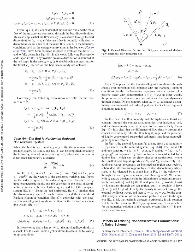
In Fig. 1, the general Riemann fan arising from a discontinuityis represented for the reduced system [Eq. (14)]. The initial leftand right states uL ¼ ðhL ρLhL ρLhLuL ÞT and uR ¼ ð hR ρRhRρRhRuRÞT are separated by two nonlinear waves (denoted by adouble line), which can be either shocks or rarefactions, wherethe smallest and largest speeds are SL and SR, respectively. Thenonlinear waves encompass an intermediate region (star region),subdivided into two subregions by a contact discontinuity whosespeed is SM (denoted by a single line in Fig. 1): the velocity u�through the star region is constant, and then SM ¼ u�. We denotewith ρ�L and ρ�R the densities in the left and right subregions, respec-tively, and with h�L and h�R the flow depths: the hydrostatic thrustp� is constant through the star region, but it is possible to haveρ�L ≠ ρ�R and h�L ≠ h�R. Finally, the density is constant through theexternal nonlinear waves, and then ρ�L ¼ ρL, ρ�R ¼ ρR. For the com-plete analytic solution of the Riemann problem related to the sys-tem [Eq. (14)], the reader is directed to Appendix I: this solutionwill be helpful when an HLLC-type approximate Riemann solverfor the numerical solution of the reduced system [Eq. (14)] is pre-sented and discussed.

Defects of Existing Nonconservative Formulations:A Naïve Scheme

In many recent references (Cao et al. 2004; Simpson and Castelltort2006; Xia et al. 2010; Zhang and Duan 2011; Li and Duffy 2011;

Fig. 1. General Riemann fan for the 1D hyperconcentrated shallowflow equations over horizontal bed

JOURNAL OF HYDRAULIC ENGINEERING © ASCE / MARCH 2014 / 257

J. Hydraul. Eng. 2014.140:254-268.

Dow

nloa

ded

from

asc

elib

rary

.org

by

DA

PS L

IBR

AR

Y o

n 02

/19/

14. C

opyr

ight

ASC

E. F

or p

erso

nal u

se o

nly;

all

righ

ts r

eser

ved.

Kim and Lee 2012), the original formulation of Eq. (1) is manip-ulated, obtaining the following system of equations:

∂h∂t þ

∂hu∂x ¼ 0

∂ρh∂t þ ∂ρhu

∂x ¼ 0

∂hu∂t þ ∂

∂x�1

2gh2 þ hu2

�¼ − 1

2gh2

ρ∂ρ∂x − gh

∂z∂x

∂z∂t ¼ 0 ð18Þ

where the bed-evolution and flow-resistance source terms havebeen temporarily discarded again. The extraction of the densityρ from the left-hand side of the momentum conservation equationintroduces a new nonconservative term ðh2ρ−1∂ρ=∂xÞ: it is pos-sible to disambiguate its mathematical meaning through disconti-nuities if a suitable regularization of the solution is chosen, but theneed to introduce an additional condition for the definition of thisnew nonconservative product is a shortcoming not present in theoriginal formulation of Eq. (1).

If the nonconservative products are not considered part of thehyperbolic problem, and are treated as smooth source terms, theleft-hand side of the system [Eq. (18)] coincides with the shallow-water equations with a passive tracer. For these equations, well-grounded and widely used numerical methods are available. Thisis why, in the cited references, the manipulation that leads to theappearance of a new nonconservative product is justified with ex-pressions such as “to use a previously developed easy numericalmethod” or “to expedite numerical solution using conservativevariables.”

In order to show the consequences of this approach, the follow-ing naïve first-order finite-volume explicit scheme is introduced:

qnþ1i ¼ qn

i − ΔtΔx

½Eðqni ;q

niþ1Þ − Eðqn

i−1;qni Þ� þ Sn

i

znþ1i ¼ zni ð19Þ

where qni ¼ ð hni ρhni huni ÞT is the vector of the cell-averaged

values of the quantities conserved in Eq. (18), calculated in theith cell of length Δx at the time level tn ¼ nΔt. In Eq. (19),Eðqn

i−1;qni Þ is the vector of the numerical fluxes calculated

using the HLLC approach summarized in Appendix (Essentialsof HLLC Approximate Riemann Solver) of Cao et al. (2004),and Sn

i is the following approximation of the right-hand sideof Eq. (18):

Sni ¼

�0 0 − gðhni Þ2

2ρni

ρniþ1 − ρni−12Δx

− ghnizniþ1 − zni−1

2Δx

�T

ð20Þ

In Eq. (20), ρni ¼ ρhni =hni is an approximation of the cell-

averaged value of the density, while zni is the cell-averaged valueof the bed elevation.

The scheme [Eqs. (19) and (20)], although only first-orderaccurate, retains the main characteristics of the models presentedin the cited references. These characteristics can be summarizedas follows:• Extraction of the density ρ from the left-hand side of the

momentum conservation equation;• Approximation of the numerical fluxes by means of a Riemann

solver for the shallow-water equations with a passive tracer(Toro 2001);

• Use of a centred finite difference scheme for the evaluationof the geometric and the density source terms at the right-hand side; and

• Inability to incorporate into the numerical scheme the actualpressure distribution at the bed step.In the next subsections, the naïve approach is verified, showing

that spurious oscillations are produced at the bed discontinuities,while the standing contact discontinuities on horizontal bed canbreak into complex systems of traveling waves. Before consideringthe consequences of the adoption of the naïve approach, it is worthmentioning the works by Wu and Wang (2007, 2008), which arebased on the scheme by Ying et al. (2004). In these works, the geo-metric source terms are upwinded and treated in a fashion similar tothat of the advective fluxes: it is easy to verify that the upwindingapproach by Ying et al. (2004) is able to reduce the spurious os-cillations on discontinuous beds, but it cannot incorporate into thenumerical scheme the actual pressure distribution at the bed step,leading to numeric solutions that are not congruent with the weaksolutions of the equations.

Verification of the Naïve Scheme: StandingContact-Discontinuity

The naïve numerical scheme [Eqs. (19) and (20)] is applied tothe case of quiescent fluid, with the following initial conditions,expressed in terms of primitive variables W ¼ ð h u ρ z ÞT :

Wðx; 0Þ ¼(WL; x < x0

WR; x > x0ð21Þ

where

WL ¼ ð 4 0 1562.5 0 ÞT ; WR ¼ ð 5 0 1000 0 ÞTð22Þ

and x0 ¼ 250 m. The channel is long L ¼ 500 m, and nonreflec-tive boundary conditions are used (Sanders 2002). For this testcase, the hydrostatic thrust is constant through the flow field: thediscontinuity at x ¼ x0 is a standing contact discontinuity over ahorizontal bed, with speed ξ ¼ 0, and the corresponding analyticalsolution is of fluid at rest.

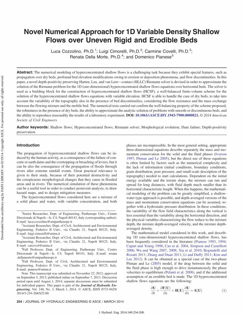
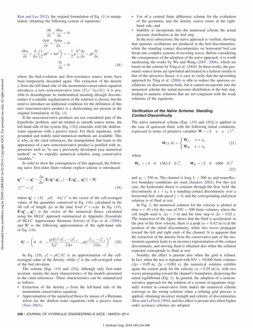
In Fig. 2, the numerical solution for the velocity is plotted attime t ¼ 10 s for the case of NV ¼ 500 finite volumes, where thecell length used is Δx ¼ 1 m and the time step is Δt ¼ 0.02 s.The inspection of the figure shows that the fluid is accelerated: inthe plot of the flow velocity, there is a peak (u ¼ 0.42 m=s) at theposition of the initial discontinuity, while two waves propagatetoward the left and right ends of the channel. It is apparent thatthe extraction of the density from the conservative part of the mo-mentum equation leads to an incorrect representation of the contactdiscontinuity, and moving fluid is obtained also when the solutionexpected corresponds to fluid at rest.

Notably, the effect is present also when the grid is refined.In fact, when the test is repeated with NV ¼ 10,000 finite volumes(Δx ¼ 0.05 m, Δt ¼ 0.001 s), the numerical solution exhibitsagain the central peak for the velocity (u ¼ 0.29 m=s), with twowaves propagating toward the channel’s boundaries, destroying theinitial equilibrium (Fig. 2). In general, the adoption of a noncon-servative approach for the solution of a system of equations origi-nally written in conservative form makes the numerical schemeconverge to the wrong solution when a refining grid process isapplied, obtaining incorrect strength and celerity of discontinuities(Hou and LeFloch 1994), and this effect is present also when higherorder accuracy schemes are adopted.

258 / JOURNAL OF HYDRAULIC ENGINEERING © ASCE / MARCH 2014

J. Hydraul. Eng. 2014.140:254-268.

Dow

nloa

ded

from

asc

elib

rary

.org

by

DA

PS L

IBR

AR

Y o

n 02

/19/

14. C

opyr

ight

ASC

E. F

or p

erso

nal u

se o

nly;

all

righ

ts r

eser

ved.

Verification of the Naïve Scheme: Dam-Break overa Step

In this test, the dam-break over a bed step considered by Begnudelliand Rosatti (2011), with hydrostatic pressure distribution on thestep, is considered. In particular, in a channel of length L ¼200 m the initial conditions [Eq. (21)] are considered, with

WL ¼ ð5 0 1165 0 ÞT ; WR ¼ ð 0.9966 0 1495 1 ÞTð23Þ

and x0 ¼ 100 m. The analytic solution (Appendix III) correspondsto fluid moving from the left to the right, passing over the bed step:the left and the right states are connected by four waves, namely,a rarefaction, a bed step discontinuity, a moving contact disconti-nuity, and finally a shock.

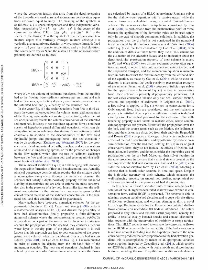
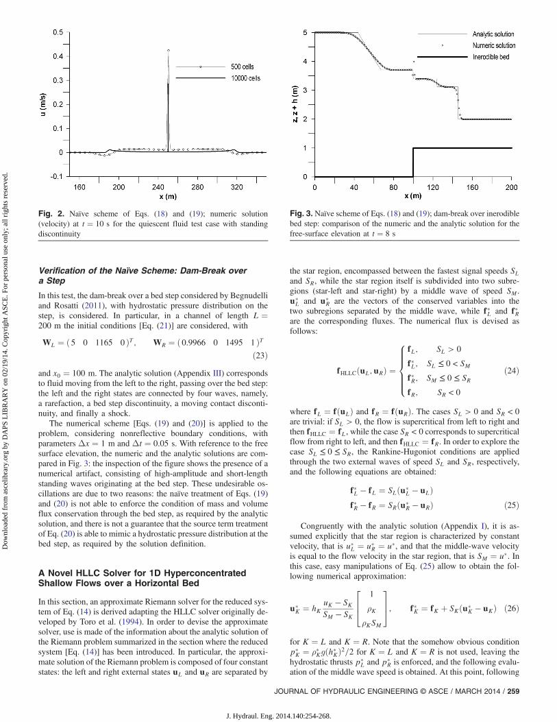
The numerical scheme [Eqs. (19) and (20)] is applied to theproblem, considering nonreflective boundary conditions, withparameters Δx ¼ 1 m and Δt ¼ 0.05 s. With reference to the freesurface elevation, the numeric and the analytic solutions are com-pared in Fig. 3: the inspection of the figure shows the presence of anumerical artifact, consisting of high-amplitude and short-lengthstanding waves originating at the bed step. These undesirable os-cillations are due to two reasons: the naïve treatment of Eqs. (19)and (20) is not able to enforce the condition of mass and volumeflux conservation through the bed step, as required by the analyticsolution, and there is not a guarantee that the source term treatmentof Eq. (20) is able to mimic a hydrostatic pressure distribution at thebed step, as required by the solution definition.

A Novel HLLC Solver for 1D HyperconcentratedShallow Flows over a Horizontal Bed

In this section, an approximate Riemann solver for the reduced sys-tem of Eq. (14) is derived adapting the HLLC solver originally de-veloped by Toro et al. (1994). In order to devise the approximatesolver, use is made of the information about the analytic solution ofthe Riemann problem summarized in the section where the reducedsystem [Eq. (14)] has been introduced. In particular, the approxi-mate solution of the Riemann problem is composed of four constantstates: the left and right external states uL and uR are separated by

the star region, encompassed between the fastest signal speeds SLand SR, while the star region itself is subdivided into two subre-gions (star-left and star-right) by a middle wave of speed SM.u�L and u�

R are the vectors of the conserved variables into thetwo subregions separated by the middle wave, while f�L and f�Rare the corresponding fluxes. The numerical flux is devised asfollows:

fHLLCðuL;uRÞ ¼

8>>>><>>>>:

fL; SL > 0

f�L; SL ≤ 0 < SM

f�R; SM ≤ 0 ≤ SR

fR; SR < 0

ð24Þ

where fL ¼ fðuLÞ and fR ¼ fðuRÞ. The cases SL > 0 and SR < 0are trivial: if SL > 0, the flow is supercritical from left to right andthen fHLLC ¼ fL, while the case SR < 0 corresponds to supercriticalflow from right to left, and then fHLLC ¼ fR. In order to explore thecase SL ≤ 0 ≤ SR, the Rankine-Hugoniot conditions are appliedthrough the two external waves of speed SL and SR, respectively,and the following equations are obtained:

f�L − fL ¼ SLðu�L − uLÞ

f�R − fR ¼ SRðu�R − uRÞ ð25Þ

Congruently with the analytic solution (Appendix I), it is as-sumed explicitly that the star region is characterized by constantvelocity, that is u�L ¼ u�R ¼ u�, and that the middle-wave velocityis equal to the flow velocity in the star region, that is SM ¼ u�. Inthis case, easy manipulations of Eq. (25) allow to obtain the fol-lowing numerical approximation:

u�K ¼ hK

uK − SKSM − SK

264

1

ρK

ρKSM

375; f�K ¼ fK þ SKðu�

K − uKÞ ð26Þ

for K ¼ L and K ¼ R. Note that the somehow obvious conditionp�K ¼ ρ�Kgðh�KÞ2=2 for K ¼ L and K ¼ R is not used, leaving the

hydrostatic thrusts p�L and p�

R is enforced, and the following evalu-ation of the middle wave speed is obtained. At this point, following

Fig. 2. Naïve scheme of Eqs. (18) and (19); numeric solution(velocity) at t ¼ 10 s for the quiescent fluid test case with standingdiscontinuity

Fig. 3. Naïve scheme of Eqs. (18) and (19); dam-break over inerodiblebed step: comparison of the numeric and the analytic solution for thefree-surface elevation at t ¼ 8 s

JOURNAL OF HYDRAULIC ENGINEERING © ASCE / MARCH 2014 / 259

J. Hydraul. Eng. 2014.140:254-268.

Dow

nloa

ded

from

asc

elib

rary

.org

by

DA

PS L

IBR

AR

Y o

n 02

/19/

14. C

opyr

ight

ASC

E. F

or p

erso

nal u

se o

nly;

all

righ

ts r

eser

ved.

Batten et al. (1997), and congruently with the analytic solution, theauthors enforce p�

L ¼ p�R, and the following evaluation of the

middle wave speed is obtained:

SM ¼ pL − pR þ ρRhRuRðSR − uRÞ þ ρLhLuLðuL − SLÞρRhRðSR − uRÞ þ ρLhLðuL − SLÞ

ð27Þ

The accuracy of the proposed numerical flux relies on the ac-curacy of the estimates for the fastest speeds SL and SR. We use thevalues proposed by Einfeldt et al. (1991)

SL ¼ minfλ1ðuLÞ; ~λ1g; SR ¼ maxfλ3ðuRÞ; ~λ3g ð28Þ

where ~λ1 ¼ uRoe − ffiffiffiffiffiffiffiffiffiffiffighRoe

pand ~λ3 ¼ uRoe þ

ffiffiffiffiffiffiffiffiffiffiffighRoe

pare calculated

using the variables uRoe and hRoe, corresponding to an intermediatestate defined as the Roe average of the left and right states. Theestimates [Eq. (28)] are intended to be a bound for the signal speedswhen a rarefaction is present, while the correct shock speed is sup-plied in the case of isolated shock.

Actually, the determination of the Roe averages for the con-served variables is not straightforward in the case of the system[Eq. (14)], and then the estimates of the primitive variables validfor the constant density Shallow-water equations are used

hRoe ¼hL þ hR

2; uRoe ¼

uRffiffiffiffiffiffihR

p þ uLffiffiffiffiffiffihL

pffiffiffiffiffiffihR

p þ ffiffiffiffiffiffihL

p ð29Þ

This choice is fully justified: Eq. (16) shows that the fluid den-sity is constant through the shocks, and then the speed estimates ofisolated shocks calculated by means of Eq. (29) are correct for thesystem [Eq. (14)].

The approximate HLLC Riemann solver proposed here exhibitsnice properties, namely, exact resolution of isolated contact discon-tinuities, exact resolution of isolated shocks, and positivity preser-vation of h and ρ: these properties are considered in Appendix II.Moreover, the Riemann solver is able to take into account the dy-namic effects through the contact discontinuity, but it is not morecomputationally expensive than the HLLC solvers used in Cao et al.(2004), Simpson and Castelltort (2006), Zhang and Duan (2011),and Kim and Lee (2012).

HCSF: A Finite-Volume Scheme for the Solutionof the 1D Hyperconcentrated Shallow FlowsEquations with Variable Bed Elevation

In the preceding section, an HLLC Riemann solver for the 1Dhyperconcentrated shallow flows over horizontal bed, where theequations are written in conservative form, has been introduced.In the present section it is described how this solver can be incor-porated into HCSF (HyperConcentrated Shallow Flows), a well-balanced finite volume scheme for the approximate solution ofEq. (1), able to take into account the effects of sediment erosionand deposition. Aiming at this, a splitting scheme is adopted: inthe first step, the hyperbolic part of Eq. (1) is considered, and thepredicted solution obtained is used as an initial condition for thecorrection step, which advances the solution in time taking intoaccount the source terms. In order to consider the space variabilityof the bed elevation z, a modified version of the Generalized hydro-static reconstruction proposed in Cozzolino et al. (2011) is used.The reconstruction adopted for the conserved variables makesthe scheme exactly well balanced at the bed discontinuities and en-sures the convergence to the correct solution when the bed issmooth, because the model falls into the class of path-conservativenumerical schemes (Parés 2006).

Prediction Step

Aiming to the solution of the hyperbolic part of Eq. (1), a first-orderfinite volume scheme is considered, and the numerical domain issubdivided into NV finite volumes of lengthΔx. If Un

i is the value,averaged over the ith cell, of the vector U at the time leveltn ¼ nΔt, the prediction step assumes the following form:

Ui ¼ Uni − Δt

Δx

�fHLLCðu−

iþ1=2;uþiþ1=2Þ − fHLLCðu−

i−1=2;uþi−1=2Þ

0

�

þ ΔtΔx

½SφðUþi−1=2;Un

i Þ þ SφðUni ;U

−iþ1=2Þ� ð30Þ

where Ui is the value of U predicted at the end of the hyperbolicstep in the ith cell. In order to calculate the numerical fluxes fHLLCand the terms Sφ, the conserved variables are reconstructed at theinterfaces. The state U−

iþ1=2, reconstructed at the left of the interfaceiþ 1=2 between the ith and the (iþ 1)th cell, is found imposingthat the state Un

i is connected to the state U−iþ1=2 by the bed-step

condition [Eq. (11)], complemented by the definition [Eq. (12)]of the thrust Pφ exerted on the step. The state Uþ

iþ1=2, reconstructedat the right of the interface iþ 1=2, is found imposing the satisfac-tion of the bed-step condition [Eq. (11)] between the states Uþ

iþ1=2and Un

iþ1, complemented by the definition [Eq. (13)] of the thrustPφ. The variables reconstruction accomplished in this manner al-lows capturing automatically the contact discontinuities containedinto the fourth characteristic field.

The values of U reconstructed at the interfaces are defined as

U−iþ1=2 ¼ ð h−iþ1=2 ρh−iþ1=2 ρhu−iþ1=2 ziþ1=2 ÞT

¼ ðu−iþ1=2 ziþ1=2 ÞT

Uþiþ1=2 ¼ ð hþiþ1=2 ρhþiþ1=2 ρhuþiþ1=2 ziþ1=2 ÞT

¼ ðuþiþ1=2 ziþ1=2 ÞT ð31Þ

where ziþ1=2 ¼ maxfzni ; zniþ1g is an unambiguous value of the bedelevation defined at the interface iþ 1=2, while u−

iþ1=2 and uþiþ1=2

are the reconstructed variables corresponding to the reduced system[Eq. (14)]. In order to show how these variables are calculated, anexample is made assuming zni ≤ zniþ1, which supplies ziþ1=2 ¼ zniþ1.Now, two different cases are possible: in the first case, the free sur-face elevation at the left of the step is less than or equal to the eleva-tion of the step top (zni þ hni ≤ zniþ1), while in the second case thefree surface elevation at the left of the step is greater than the eleva-tion of the step top (zni þ hni > zniþ1).

In the case that zni þ hni ≤ zniþ1, the values of the variables recon-structed at the left of the interface are simply h−iþ1=2 ¼ 0, ρ−iþ1=2 ¼ 0

and hu−iþ1=2 ¼ 0. In the case zni þ hni > zniþ1, the bed-step condition[Eq. (11)], applied between the states Un

i and U−iþ1=2, supplies

ρ−iþ1=2 ¼ ρni and hu−iþ1=2 ¼ huni , while the reconstructed value ofthe flow depth is found solving the following equation with respectto h−iþ1=2:

ðhuni Þ2hni

þ g2ðhni þ zni − ziþ1=2Þ2 ¼

g2ðh−iþ1=2Þ2 þ

ðhu−iþ1=2Þ2h−iþ1=2

ð32Þ

Eq. (32) can exhibit two, one, or no positive real solution forh−iþ1=2. When two distinct solutions are available, one solutioncorresponds to subcritical conditions, while the other correspondsto supercritical conditions: in this case, the right state U−

iþ1=2 ischosen in order to keep the same flow conditions (sub- or super-critical) of the left state Un

i . When only one solution is available,the state U−

iþ1=2 corresponds to critical flow, and this solution is

260 / JOURNAL OF HYDRAULIC ENGINEERING © ASCE / MARCH 2014

J. Hydraul. Eng. 2014.140:254-268.

Dow

nloa

ded

from

asc

elib

rary

.org

by

DA

PS L

IBR

AR

Y o

n 02

/19/

14. C

opyr

ight

ASC

E. F

or p

erso

nal u

se o

nly;

all

righ

ts r

eser

ved.

retained. Finally, the case of no positive real solution has a clearphysical meaning: the residual total force Ri ¼ ðhuni Þ2=hni þgðhni þ zni − ziþ1=2Þ2 is not sufficient to make the discharge passover the bed step. In these conditions, the Bélanger’s principleis applied, and critical state conditions are imposed at the bed-steptop

h−iþ1=2 ¼ffiffiffiffiffiffiffi2Ri

3g

s; hu−iþ1=2 ¼

hunijhuni j

h−iþ1=2

ffiffiffiffiffiffiffiffiffiffiffiffiffiffigh−iþ1=2

qρ−iþ1=2 ¼ ρni ð33Þ

Once that the state U−iþ1=2 is known, the thrust acting on the bed

step is calculated as PϕðUni ;U

−iþ1=2Þ ¼ gρi½ðhni Þ2 − α2�=2, where

α ¼ maxf0; hni þ zni − ziþ1=2g, and the vector SφðUni ;U

−iþ1=2Þ

can be finally calculated from Eq. (8). At the right of the bedstep, the application of the bed-step condition [Eq. (11)] betweenthe states Uþ

iþ1=2 and Uniþ1, complemented with the definition

[Eq. (13)], supplies the reconstructed values hþiþ1=2 ¼ hniþ1,

ρþiþ1=2 ¼ ρniþ1, and huþiþ1=2 ¼ huniþ1, together with PφðUþiþ1=2;

Uniþ1Þ ¼ 0, and then the vector SφðUþ

iþ1=2;Uniþ1Þ is identically null.

In the case that zni > zniþ1, the same procedure is used, with theobvious changes.

In order to cope with dry areas, a limit fluid depth εh is defined,and the cells where h < εh are considered dry. The velocity is setto zero into the dry cells and the momentum equation is notadjourned, while fluxes between two dry cells are set to zero.At the interface between a wet and a dry cell, the analyticspeed estimates given by Fraccarollo and Toro (1995) are used(Appendix II), instead of the estimates [Eq. (28)]. The lengthΔt of the time step must be limited, because the prediction stepis explicit, and the algorithm is conditionally stable. While theapproximate Riemann solver used for the problem with horizontalbeds is positive preserving, there is no guarantee that this propertyis satisfied also when the bed elevation is variable, and the citedreconstructions are accomplished. Nonetheless, the numerical ex-periments show that the numerical scheme behaves nicely, and nonegative depth appears, if the classic half Courant-Friderichs-Levycondition is satisfied (Bouchut 2004).

Correction Step

Once that the predicted value Ui of the conserved variable U isavailable, the correction step is accomplished in order to considerthe presence of source terms (friction, mass exchange between theflow and the saturated bed, and bed evolution in time). We considera first-order implicit algorithm (Burguete et al. 2007; Cozzolinoet al. 2012), in order to avoid time step restrictions and en-hance the stability of the algorithm in presence of wetting-dryingmoving fronts

Unþ1i − SðUnþ1

i ÞΔt ¼ Ui ð34Þwhere SðUnþ1

i Þ is the vector source term from Eq. (2). Due to thenonlinearity of the source terms, the Newton-Raphson algorithm isadopted for the solution of Eq. (34).

If the mixture depth falls below the limit depth εh, it is assumedthat the flow is not able to carry the sediment. In this case,the velocity is set to zero, the sediment carried is settledcompletely, and the bed elevation is adjourned. Accordingly, themixture density is set equal to the water density and the flow depthis recalculated in order to satisfy mass conservation in the cell(Armanini et al. 2009).

Numerical Experiments

In this section, the HCSF scheme is demonstrated by means of se-lected numerical tests. The first battery of tests explores the abilityof the HLLC solver proposed in this work to approximate transientsolutions, to preserve nontrivial equilibria on horizontal beds, andto allow the flow propagation on dry beds without the formationof negative depths and densities. The second battery of tests ex-plores the integration between the Riemann solver and a suitablereconstruction of conserved variables, devised in order to take intoaccount properly the variability of the bed elevation, also when thisis discontinuous. A final test is devoted to verify the applicabilityof HCSF in a realistic case. In all the numerical tests, the valueg ¼ 9.81 m=s2 is used.

Quiescent Fluid with Standing Discontinuity

The numerical test of quiescent fluid with standing contact discon-tinuity is repeated using the HCSF scheme, with N ¼ 500 finitevolumes (Δx ¼ 1 m,Δt ¼ 0.02 s), setting the source term SðUÞ tozero. The simulation proves that at time t ¼ 2,000 s the velocity iszero to within round-off error, as expected for the quiescent fluidsolution, also when very long runs are considered.

It is instructive to compare this result with those obtained bythe naïve scheme of Eqs. (19) and (20), and contained in Fig. 2:the HLLC Riemann solver described in this paper is able to capturestanding contact discontinuities at the machine precision level, dis-criminating the dynamic effects through the middle wave. Existingmethods, based on nonconservative manipulations of the originalEq. (1), do not exhibit this property.

Dam-Break over Horizontal Bed

The second numerical test is devoted to verifying the ability of theHLLC Riemann solver to approximate the numerical solution ofa Riemann problem where different types of waves are present.Aiming at this, the HCSF scheme is applied, considering a horizon-tal channel of length L ¼ 500 m and using the initial conditions ofEq. (21), with

WL ¼ ð 10 0 1562.5 0 Þ; WR ¼ ð 1 0 1000 0 Þð35Þ

and xo ¼ 250 m. Again, the effects of erosion, deposition, and fric-tion are neglected, and then the source term SðUÞ is set to zero. Theanalytic solution of this Riemann problem can be found with themethods described in Appendix I: the initial discontinuity breaksinto a shock propagating toward the right, and a rarefaction wavepropagating toward the left. The two extreme waves encompasstwo constant states separated by a moving contact discontinuity.

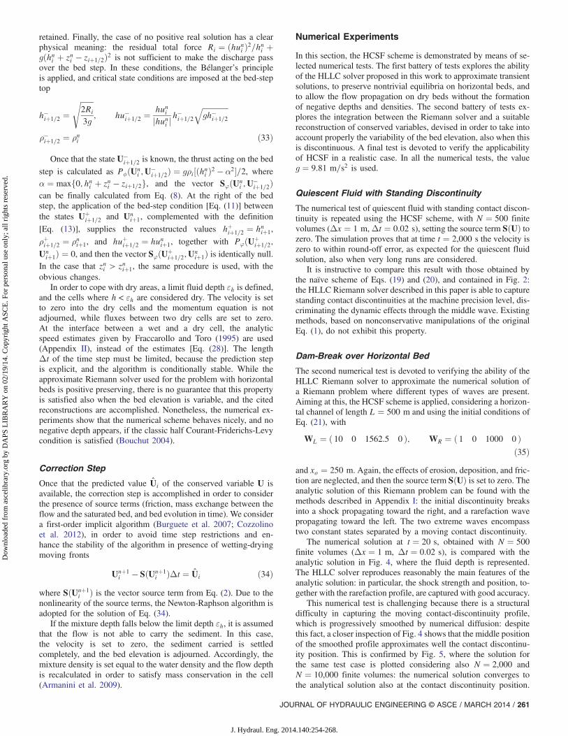
The numerical solution at t ¼ 20 s, obtained with N ¼ 500finite volumes (Δx ¼ 1 m, Δt ¼ 0.02 s), is compared with theanalytic solution in Fig. 4, where the fluid depth is represented.The HLLC solver reproduces reasonably the main features of theanalytic solution: in particular, the shock strength and position, to-gether with the rarefaction profile, are captured with good accuracy.

This numerical test is challenging because there is a structuraldifficulty in capturing the moving contact-discontinuity profile,which is progressively smoothed by numerical diffusion: despitethis fact, a closer inspection of Fig. 4 shows that the middle positionof the smoothed profile approximates well the contact discontinu-ity position. This is confirmed by Fig. 5, where the solution forthe same test case is plotted considering also N ¼ 2,000 andN ¼ 10,000 finite volumes: the numerical solution converges tothe analytical solution also at the contact discontinuity position.

JOURNAL OF HYDRAULIC ENGINEERING © ASCE / MARCH 2014 / 261

J. Hydraul. Eng. 2014.140:254-268.

Dow

nloa

ded

from

asc

elib

rary

.org

by

DA

PS L

IBR

AR

Y o

n 02

/19/

14. C

opyr

ight

ASC

E. F

or p

erso

nal u

se o

nly;

all

righ

ts r

eser

ved.

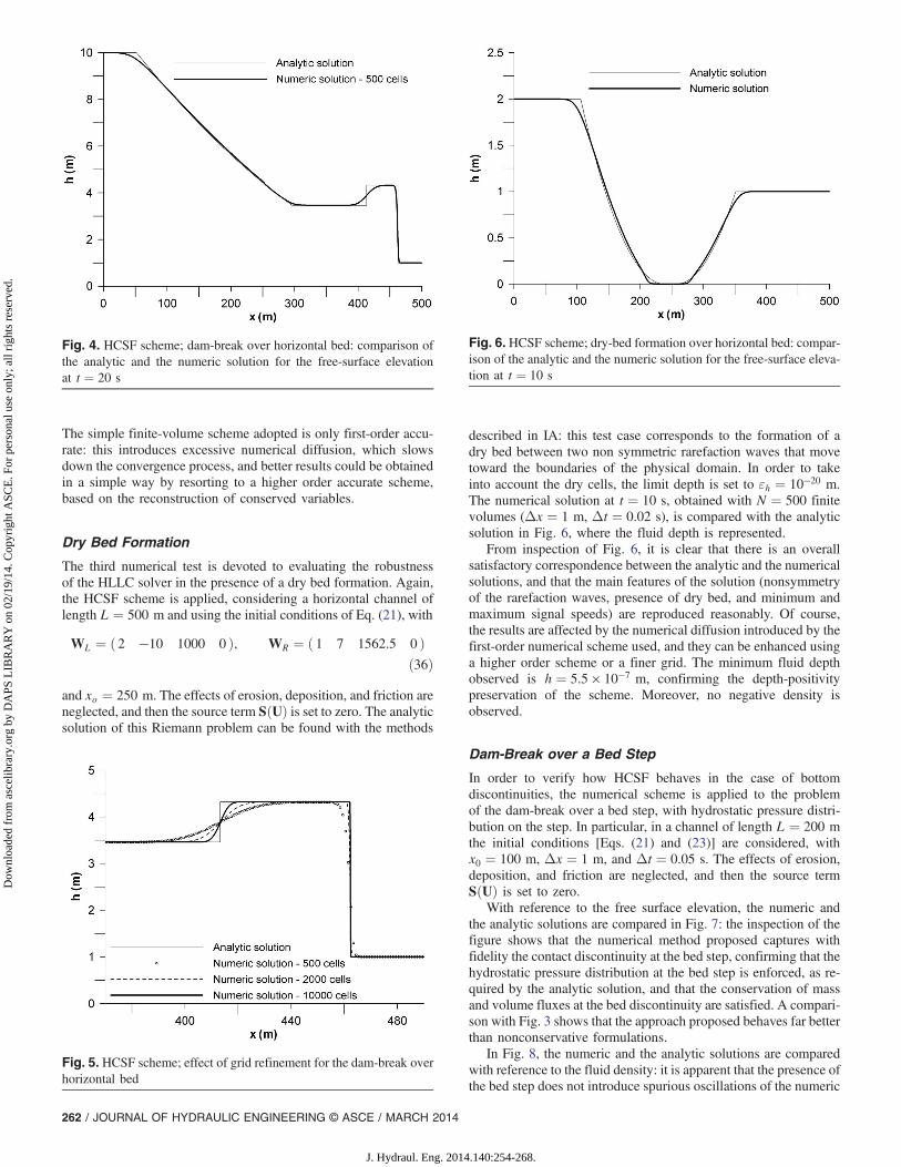
The simple finite-volume scheme adopted is only first-order accu-rate: this introduces excessive numerical diffusion, which slowsdown the convergence process, and better results could be obtainedin a simple way by resorting to a higher order accurate scheme,based on the reconstruction of conserved variables.

Dry Bed Formation

The third numerical test is devoted to evaluating the robustnessof the HLLC solver in the presence of a dry bed formation. Again,the HCSF scheme is applied, considering a horizontal channel oflength L ¼ 500 m and using the initial conditions of Eq. (21), with

WL ¼ ð 2 −10 1000 0 Þ; WR ¼ ð 1 7 1562.5 0 Þð36Þ

and xo ¼ 250 m. The effects of erosion, deposition, and friction areneglected, and then the source term SðUÞ is set to zero. The analyticsolution of this Riemann problem can be found with the methods

described in IA: this test case corresponds to the formation of adry bed between two non symmetric rarefaction waves that movetoward the boundaries of the physical domain. In order to takeinto account the dry cells, the limit depth is set to εh ¼ 10−20 m.The numerical solution at t ¼ 10 s, obtained with N ¼ 500 finitevolumes (Δx ¼ 1 m, Δt ¼ 0.02 s), is compared with the analyticsolution in Fig. 6, where the fluid depth is represented.

From inspection of Fig. 6, it is clear that there is an overallsatisfactory correspondence between the analytic and the numericalsolutions, and that the main features of the solution (nonsymmetryof the rarefaction waves, presence of dry bed, and minimum andmaximum signal speeds) are reproduced reasonably. Of course,the results are affected by the numerical diffusion introduced by thefirst-order numerical scheme used, and they can be enhanced usinga higher order scheme or a finer grid. The minimum fluid depthobserved is h ¼ 5.5 × 10−7 m, confirming the depth-positivitypreservation of the scheme. Moreover, no negative density isobserved.

Dam-Break over a Bed Step

In order to verify how HCSF behaves in the case of bottomdiscontinuities, the numerical scheme is applied to the problemof the dam-break over a bed step, with hydrostatic pressure distri-bution on the step. In particular, in a channel of length L ¼ 200 mthe initial conditions [Eqs. (21) and (23)] are considered, withx0 ¼ 100 m, Δx ¼ 1 m, and Δt ¼ 0.05 s. The effects of erosion,deposition, and friction are neglected, and then the source termSðUÞ is set to zero.

With reference to the free surface elevation, the numeric andthe analytic solutions are compared in Fig. 7: the inspection of thefigure shows that the numerical method proposed captures withfidelity the contact discontinuity at the bed step, confirming that thehydrostatic pressure distribution at the bed step is enforced, as re-quired by the analytic solution, and that the conservation of massand volume fluxes at the bed discontinuity are satisfied. A compari-son with Fig. 3 shows that the approach proposed behaves far betterthan nonconservative formulations.

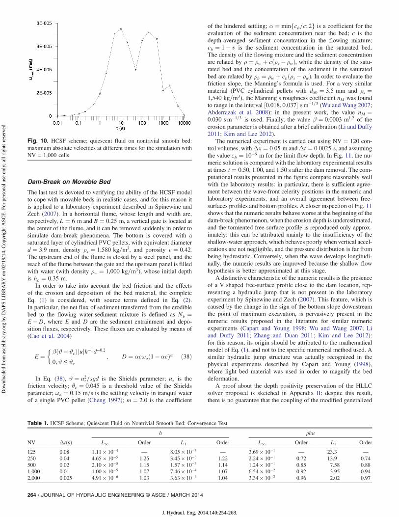
In Fig. 8, the numeric and the analytic solutions are comparedwith reference to the fluid density: it is apparent that the presence ofthe bed step does not introduce spurious oscillations of the numeric

Fig. 4. HCSF scheme; dam-break over horizontal bed: comparison ofthe analytic and the numeric solution for the free-surface elevationat t ¼ 20 s

Fig. 5. HCSF scheme; effect of grid refinement for the dam-break overhorizontal bed

Fig. 6. HCSF scheme; dry-bed formation over horizontal bed: compar-ison of the analytic and the numeric solution for the free-surface eleva-tion at t ¼ 10 s

262 / JOURNAL OF HYDRAULIC ENGINEERING © ASCE / MARCH 2014

J. Hydraul. Eng. 2014.140:254-268.

Dow

nloa

ded

from

asc

elib

rary

.org

by

DA

PS L

IBR

AR

Y o

n 02

/19/

14. C

opyr

ight

ASC

E. F

or p

erso

nal u

se o

nly;

all

righ

ts r

eser

ved.

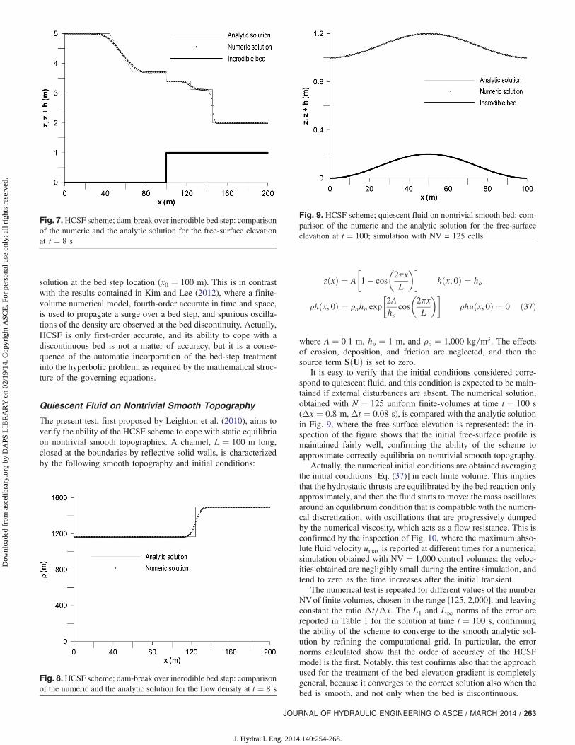
solution at the bed step location (x0 ¼ 100 m). This is in contrastwith the results contained in Kim and Lee (2012), where a finite-volume numerical model, fourth-order accurate in time and space,is used to propagate a surge over a bed step, and spurious oscilla-tions of the density are observed at the bed discontinuity. Actually,HCSF is only first-order accurate, and its ability to cope with adiscontinuous bed is not a matter of accuracy, but it is a conse-quence of the automatic incorporation of the bed-step treatmentinto the hyperbolic problem, as required by the mathematical struc-ture of the governing equations.

Quiescent Fluid on Nontrivial Smooth Topography

The present test, first proposed by Leighton et al. (2010), aims toverify the ability of the HCSF scheme to cope with static equilibriaon nontrivial smooth topographies. A channel, L ¼ 100 m long,closed at the boundaries by reflective solid walls, is characterizedby the following smooth topography and initial conditions:

zðxÞ ¼ A

�1 − cos

�2πxL

��hðx; 0Þ ¼ ho

ρhðx; 0Þ ¼ ρoho exp

�2Aho

cos

�2πxL

��ρhuðx; 0Þ ¼ 0 ð37Þ

where A ¼ 0.1 m, ho ¼ 1 m, and ρo ¼ 1,000 kg=m3. The effectsof erosion, deposition, and friction are neglected, and then thesource term SðUÞ is set to zero.

It is easy to verify that the initial conditions considered corre-spond to quiescent fluid, and this condition is expected to be main-tained if external disturbances are absent. The numerical solution,obtained with N ¼ 125 uniform finite-volumes at time t ¼ 100 s(Δx ¼ 0.8 m,Δt ¼ 0.08 s), is compared with the analytic solutionin Fig. 9, where the free surface elevation is represented: the in-spection of the figure shows that the initial free-surface profile ismaintained fairly well, confirming the ability of the scheme toapproximate correctly equilibria on nontrivial smooth topography.

Actually, the numerical initial conditions are obtained averagingthe initial conditions [Eq. (37)] in each finite volume. This impliesthat the hydrostatic thrusts are equilibrated by the bed reaction onlyapproximately, and then the fluid starts to move: the mass oscillatesaround an equilibrium condition that is compatible with the numeri-cal discretization, with oscillations that are progressively dumpedby the numerical viscosity, which acts as a flow resistance. This isconfirmed by the inspection of Fig. 10, where the maximum abso-lute fluid velocity umax is reported at different times for a numericalsimulation obtained with NV ¼ 1,000 control volumes: the veloc-ities obtained are negligibly small during the entire simulation, andtend to zero as the time increases after the initial transient.

The numerical test is repeated for different values of the numberNVof finite volumes, chosen in the range [125, 2,000], and leavingconstant the ratio Δt=Δx. The L1 and L∞ norms of the error arereported in Table 1 for the solution at time t ¼ 100 s, confirmingthe ability of the scheme to converge to the smooth analytic sol-ution by refining the computational grid. In particular, the errornorms calculated show that the order of accuracy of the HCSFmodel is the first. Notably, this test confirms also that the approachused for the treatment of the bed elevation gradient is completelygeneral, because it converges to the correct solution also when thebed is smooth, and not only when the bed is discontinuous.

Fig. 7.HCSF scheme; dam-break over inerodible bed step: comparisonof the numeric and the analytic solution for the free-surface elevationat t ¼ 8 s

Fig. 8.HCSF scheme; dam-break over inerodible bed step: comparisonof the numeric and the analytic solution for the flow density at t ¼ 8 s

Fig. 9. HCSF scheme; quiescent fluid on nontrivial smooth bed: com-parison of the numeric and the analytic solution for the free-surfaceelevation at t ¼ 100; simulation with NV = 125 cells

JOURNAL OF HYDRAULIC ENGINEERING © ASCE / MARCH 2014 / 263

J. Hydraul. Eng. 2014.140:254-268.

Dow

nloa

ded

from

asc

elib

rary

.org

by

DA

PS L

IBR

AR

Y o

n 02

/19/

14. C

opyr

ight

ASC

E. F

or p

erso

nal u

se o

nly;

all

righ

ts r

eser

ved.

Dam-Break on Movable Bed

The last test is devoted to verifying the ability of the HCSF modelto cope with movable beds in realistic cases, and for this reason itis applied to a laboratory experiment described in Spinewine andZech (2007). In a horizontal flume, whose length and width are,respectively, L ¼ 6 m and B ¼ 0.25 m, a vertical gate is located atthe center of the flume, and it can be removed suddenly in order tosimulate dam-break phenomena. The bottom is covered with asaturated layer of cylindrical PVC pellets, with equivalent diameterd ¼ 3.9 mm, density ρs ¼ 1,580 kg=m3, and porosity v ¼ 0.42.The upstream end of the flume is closed by a steel panel, and thereach of the flume between the gate and the upstream panel is filledwith water (with density ρw ¼ 1,000 kg=m3), whose initial depthis ho ¼ 0.35 m.

In order to take into account the bed friction and the effectsof the erosion and deposition of the bed material, the completeEq. (1) is considered, with source terms defined in Eq. (2).In particular, the net flux of sediment transferred from the erodiblebed to the flowing water-sediment mixture is defined as Nb ¼E −D, where E and D are the sediment entrainment and depo-sition fluxes, respectively. These fluxes are evaluated by means of(Cao et al. 2004)

E ¼�βðϑ − ϑcÞjujh−1d−0.20;ϑ ≤ ϑc

; D ¼ αcωoð1 − αcÞm ð38Þ

In Eq. (38), ϑ ¼ u2�=sgd is the Shields parameter; u� is thefriction velocity; θc ¼ 0.045 is a threshold value of the Shieldsparameter; ωo ¼ 0.15 m=s is the settling velocity in tranquil waterof a single PVC pellet (Cheng 1997); m ¼ 2.0 is the coefficient

of the hindered settling; α ¼ minfcb=c; 2g is a coefficient for theevaluation of the sediment concentration near the bed; c is thedepth-averaged sediment concentration in the flowing mixture;cb ¼ 1 − v is the sediment concentration in the saturated bed.The density of the flowing mixture and the sediment concentrationare related by ρ ¼ ρw þ cðρs − ρwÞ, while the density of the satu-rated bed and the concentration of the sediment in the saturatedbed are related by ρb ¼ ρw þ cbðρs − ρwÞ. In order to evaluate thefriction slope, the Manning’s formula is used. For a very similarmaterial (PVC cylindrical pellets with d50 ¼ 3.5 mm and ρs ¼1,540 kg=m3), the Manning’s roughness coefficient nM was foundto range in the interval ½0.018; 0.037� sm−1=3 (Wu and Wang 2007;Abderrazak et al. 2008): in the present work, the value nM ¼0.030 sm−1=3 is used. Finally, the value β ¼ 0.0003 m1.2 of theerosion parameter is obtained after a brief calibration (Li and Duffy2011; Kim and Lee 2012).

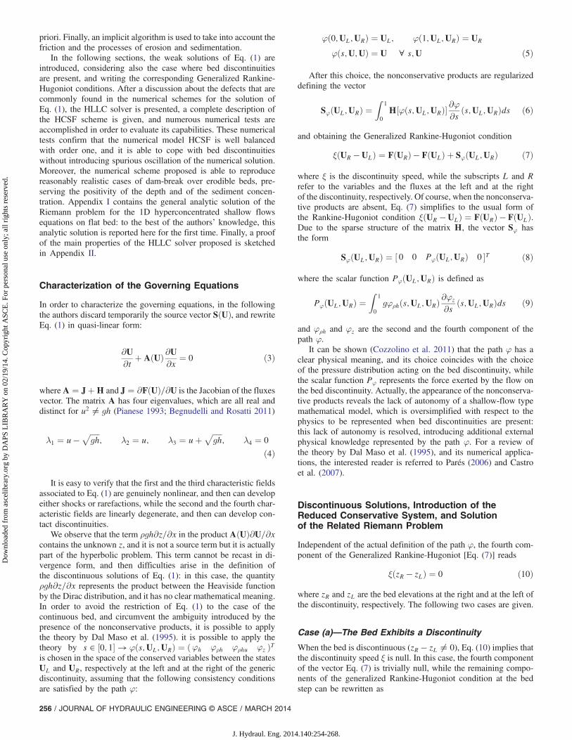
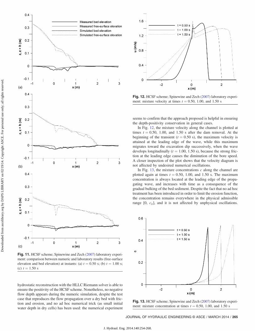
The numerical experiment is carried out using NV ¼ 120 con-trol volumes, withΔx ¼ 0.05 m andΔt ¼ 0.0025 s, and assumingthe value εh ¼ 10−6 m for the limit flow depth. In Fig. 11, the nu-meric solution is compared with the laboratory experimental resultsat times t ¼ 0.50, 1.00, and 1.50 s after the dam removal. The com-putational results presented in the figure compare reasonably wellwith the laboratory results: in particular, there is sufficient agree-ment between the wave-front celerity positions in the numeric andlaboratory experiments, and an overall agreement between free-surfaces profiles and bottom profiles. A closer inspection of Fig. 11shows that the numeric results behave worse at the beginning of thedam-break phenomenon, when the erosion depth is underestimated,and the tormented free-surface profile is reproduced only approx-imately: this can be attributed mainly to the insufficiency of theshallow-water approach, which behaves poorly when vertical accel-erations are not negligible, and the pressure distribution is far frombeing hydrostatic. Conversely, when the wave develops longitudi-nally, the numeric results are improved because the shallow flowhypothesis is better approximated at this stage.

A distinctive characteristic of the numeric results is the presenceof a V shaped free-surface profile close to the dam location, rep-resenting a hydraulic jump that is not present in the laboratoryexperiment by Spinewine and Zech (2007). This feature, which iscaused by the change in the sign of the bottom slope downstreamthe point of maximum excavation, is pervasively present in thenumeric results proposed in the literature for similar numericexperiments (Capart and Young 1998; Wu and Wang 2007; Liand Duffy 2011; Zhang and Duan 2011; Kim and Lee 2012):for this reason, its origin should be attributed to the mathematicalmodel of Eq. (1), and not to the specific numerical method used. Asimilar hydraulic jump structure was actually recognized in thephysical experiments described by Capart and Young (1998),where light bed material was used in order to magnify the beddeformation.

A proof about the depth positivity preservation of the HLLCsolver proposed is sketched in Appendix II: despite this result,there is no guarantee that the coupling of the modified generalized

Fig. 10. HCSF scheme; quiescent fluid on nontrivial smooth bed:maximum absolute velocities at different times for the simulation withNV = 1,000 cells

Table 1. HCSF Scheme; Quiescent Fluid on Nontrivial Smooth Bed: Convergence Test

NV ΔtðsÞh ρhu

L∞ Order L1 Order L∞ Order L1 Order

125 0.08 1.11 × 10−4 — 8.05 × 10−3 — 3.69 × 10−1 — 23.3 —250 0.04 4.65 × 10−5 1.25 3.45 × 10−3 1.22 2.24 × 10−1 0.72 13.9 0.74500 0.02 2.10 × 10−5 1.15 1.57 × 10−3 1.14 1.24 × 10−1 0.85 7.58 0.881,000 0.01 1.00 × 10−5 1.07 7.46 × 10−4 1.07 6.54 × 10−2 0.92 3.95 0.942,000 0.005 4.91 × 10−6 1.03 3.63 × 10−4 1.04 3.34 × 10−2 0.96 2.02 0.97

264 / JOURNAL OF HYDRAULIC ENGINEERING © ASCE / MARCH 2014

J. Hydraul. Eng. 2014.140:254-268.

Dow

nloa

ded

from

asc

elib

rary

.org

by

DA

PS L

IBR

AR

Y o

n 02

/19/

14. C

opyr

ight

ASC

E. F

or p

erso

nal u

se o

nly;

all

righ

ts r

eser

ved.

hydrostatic reconstruction with the HLLC Riemann solver is able toensure the positivity of the HCSF scheme. Nonetheless, no negativeflow depth appears during the numeric simulation, despite the testcase that reproduces the flow propagation over a dry bed with fric-tion and erosion, and no ad hoc numerical trick (as small initialwater depth in dry cells) has been used: the numerical experiment

seems to confirm that the approach proposed is helpful in ensuringthe depth-positivity conservation in general cases.

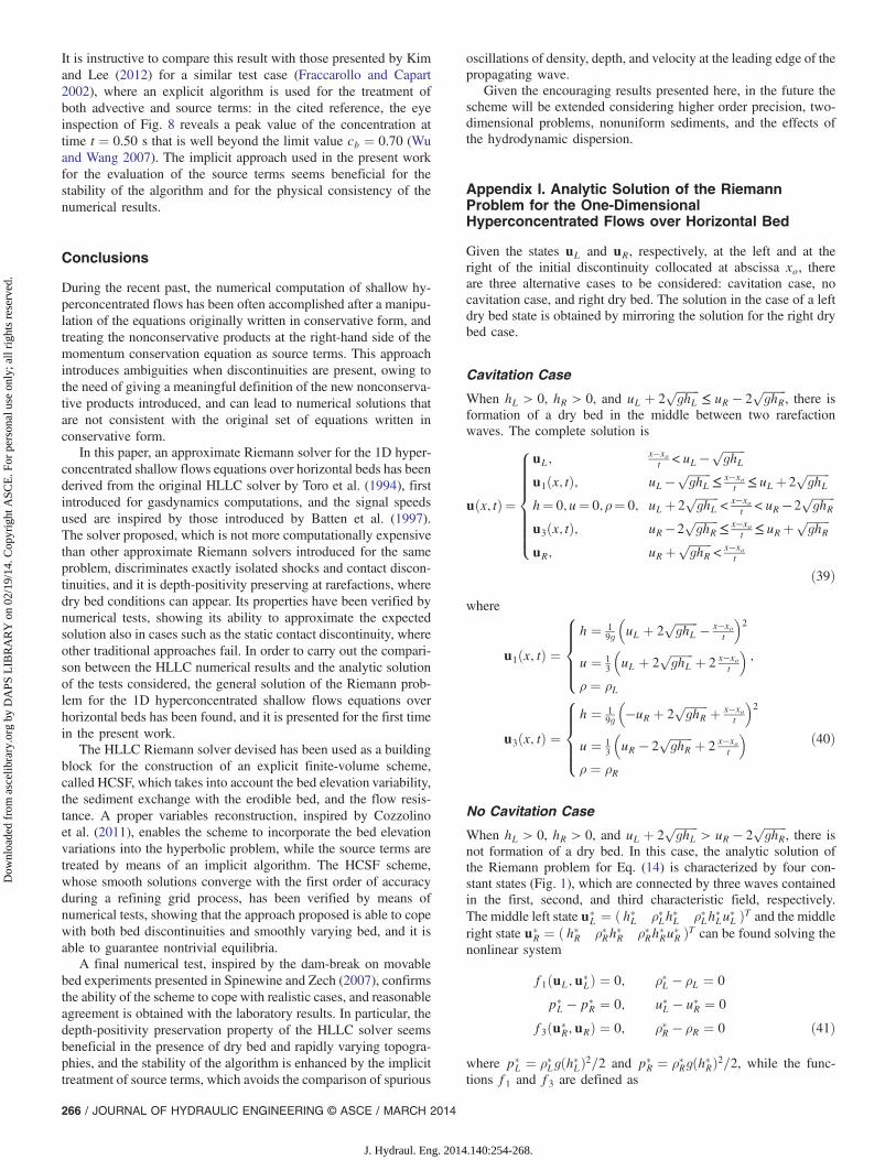
In Fig. 12, the mixture velocity along the channel is plotted attimes t ¼ 0.50, 1.00, and 1.50 s after the dam removal. At thebeginning of the transient (t ¼ 0.50 s), the maximum velocity isattained at the leading edge of the wave, while this maximummigrates toward the excavation dip successively, when the wavedevelops longitudinally (t ¼ 1.00, 1.50 s), because the strong fric-tion at the leading edge causes the diminution of the bore speed.A closer inspection of the plot shows that the velocity diagram isnot affected by undesired numerical oscillations.

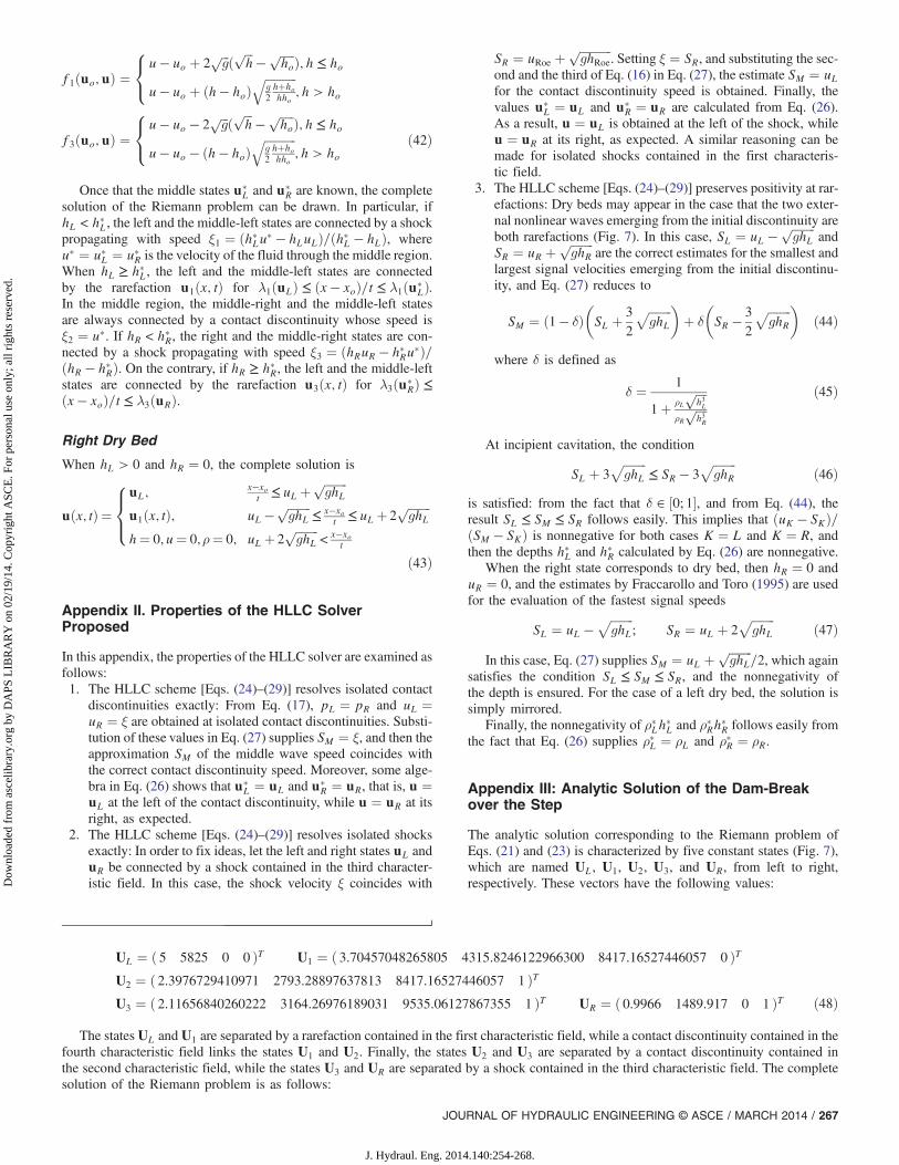
In Fig. 13, the mixture concentrations c along the channel areplotted again at times t ¼ 0.50, 1.00, and 1.50 s. The maximumconcentration is always located at the leading edge of the propa-gating wave, and increases with time as a consequence of thegradual bulking of the bed sediment. Despite the fact that no ad hoctreatment has been introduced in order to limit the erosion function,the concentration remains everywhere in the physical admissiblerange [0, cb], and it is not affected by unphysical oscillations.

Fig. 11. HCSF scheme; Spinewine and Zech (2007) laboratory experi-ment: comparison between numeric and laboratory results (free-surfaceelevation and bed elevation) at instants: (a) t ¼ 0.50 s; (b) t ¼ 1.00 s;(c) t ¼ 1.50 s

Fig. 12. HCSF scheme; Spinewine and Zech (2007) laboratory experi-ment: mixture velocity at times t ¼ 0.50, 1.00, and 1.50 s

Fig. 13. HCSF scheme; Spinewine and Zech (2007) laboratory experi-ment: mixture concentration at times t ¼ 0.50, 1.00, and 1.50 s

JOURNAL OF HYDRAULIC ENGINEERING © ASCE / MARCH 2014 / 265

J. Hydraul. Eng. 2014.140:254-268.

Dow

nloa

ded

from

asc

elib

rary

.org

by

DA

PS L

IBR

AR

Y o

n 02

/19/

14. C

opyr

ight

ASC

E. F

or p

erso

nal u

se o

nly;

all

righ

ts r

eser

ved.

It is instructive to compare this result with those presented by Kimand Lee (2012) for a similar test case (Fraccarollo and Capart2002), where an explicit algorithm is used for the treatment ofboth advective and source terms: in the cited reference, the eyeinspection of Fig. 8 reveals a peak value of the concentration attime t ¼ 0.50 s that is well beyond the limit value cb ¼ 0.70 (Wuand Wang 2007). The implicit approach used in the present workfor the evaluation of the source terms seems beneficial for thestability of the algorithm and for the physical consistency of thenumerical results.

Conclusions

During the recent past, the numerical computation of shallow hy-perconcentrated flows has been often accomplished after a manipu-lation of the equations originally written in conservative form, andtreating the nonconservative products at the right-hand side of themomentum conservation equation as source terms. This approachintroduces ambiguities when discontinuities are present, owing tothe need of giving a meaningful definition of the new nonconserva-tive products introduced, and can lead to numerical solutions thatare not consistent with the original set of equations written inconservative form.

In this paper, an approximate Riemann solver for the 1D hyper-concentrated shallow flows equations over horizontal beds has beenderived from the original HLLC solver by Toro et al. (1994), firstintroduced for gasdynamics computations, and the signal speedsused are inspired by those introduced by Batten et al. (1997).The solver proposed, which is not more computationally expensivethan other approximate Riemann solvers introduced for the sameproblem, discriminates exactly isolated shocks and contact discon-tinuities, and it is depth-positivity preserving at rarefactions, wheredry bed conditions can appear. Its properties have been verified bynumerical tests, showing its ability to approximate the expectedsolution also in cases such as the static contact discontinuity, whereother traditional approaches fail. In order to carry out the compari-son between the HLLC numerical results and the analytic solutionof the tests considered, the general solution of the Riemann prob-lem for the 1D hyperconcentrated shallow flows equations overhorizontal beds has been found, and it is presented for the first timein the present work.

The HLLC Riemann solver devised has been used as a buildingblock for the construction of an explicit finite-volume scheme,called HCSF, which takes into account the bed elevation variability,the sediment exchange with the erodible bed, and the flow resis-tance. A proper variables reconstruction, inspired by Cozzolinoet al. (2011), enables the scheme to incorporate the bed elevationvariations into the hyperbolic problem, while the source terms aretreated by means of an implicit algorithm. The HCSF scheme,whose smooth solutions converge with the first order of accuracyduring a refining grid process, has been verified by means ofnumerical tests, showing that the approach proposed is able to copewith both bed discontinuities and smoothly varying bed, and it isable to guarantee nontrivial equilibria.

A final numerical test, inspired by the dam-break on movablebed experiments presented in Spinewine and Zech (2007), confirmsthe ability of the scheme to cope with realistic cases, and reasonableagreement is obtained with the laboratory results. In particular, thedepth-positivity preservation property of the HLLC solver seemsbeneficial in the presence of dry bed and rapidly varying topogra-phies, and the stability of the algorithm is enhanced by the implicittreatment of source terms, which avoids the comparison of spurious

oscillations of density, depth, and velocity at the leading edge of thepropagating wave.

Given the encouraging results presented here, in the future thescheme will be extended considering higher order precision, two-dimensional problems, nonuniform sediments, and the effects ofthe hydrodynamic dispersion.

Appendix I. Analytic Solution of the RiemannProblem for the One-DimensionalHyperconcentrated Flows over Horizontal Bed

Given the states uL and uR, respectively, at the left and at theright of the initial discontinuity collocated at abscissa xo, thereare three alternative cases to be considered: cavitation case, nocavitation case, and right dry bed. The solution in the case of a leftdry bed state is obtained by mirroring the solution for the right drybed case.

Cavitation Case

When hL > 0, hR > 0, and uL þ 2ffiffiffiffiffiffiffiffighL

p ≤ uR − 2ffiffiffiffiffiffiffiffighR

p, there is

formation of a dry bed in the middle between two rarefactionwaves. The complete solution is

uðx; tÞ ¼

8>>>>>>><>>>>>>>:

uL;x−xot < uL− ffiffiffiffiffiffiffiffi

ghLp

u1ðx; tÞ; uL− ffiffiffiffiffiffiffiffighL

p ≤ x−xot ≤ uLþ 2

ffiffiffiffiffiffiffiffighL

p

h¼ 0;u¼ 0;ρ¼ 0; uLþ 2ffiffiffiffiffiffiffiffighL

p< x−xo

t < uR− 2ffiffiffiffiffiffiffiffighR

p

u3ðx; tÞ; uR− 2ffiffiffiffiffiffiffiffighR

p ≤ x−xot ≤ uRþ

ffiffiffiffiffiffiffiffighR

p

uR; uRþffiffiffiffiffiffiffiffighR

p< x−xo

t

ð39Þwhere

u1ðx; tÞ ¼

8>>><>>>:

h ¼ 19g

�uL þ 2

ffiffiffiffiffiffiffiffighL

p − x−xot

�2

u ¼ 13

�uL þ 2

ffiffiffiffiffiffiffiffighL

p þ 2 x−xot

�ρ ¼ ρL

;

u3ðx; tÞ ¼

8>>><>>>:

h ¼ 19g

�−uR þ 2

ffiffiffiffiffiffiffiffighR

p þ x−xot

�2

u ¼ 13

�uR − 2

ffiffiffiffiffiffiffiffighR

p þ 2 x−xot

�ρ ¼ ρR

ð40Þ

No Cavitation Case

When hL > 0, hR > 0, and uL þ 2ffiffiffiffiffiffiffiffighL

p> uR − 2

ffiffiffiffiffiffiffiffighR

p, there is

not formation of a dry bed. In this case, the analytic solution ofthe Riemann problem for Eq. (14) is characterized by four con-stant states (Fig. 1), which are connected by three waves containedin the first, second, and third characteristic field, respectively.The middle left state u�

L ¼ ð h�L ρ�Lh�L ρ�Lh

�Lu

�L ÞT and the middle

right state u�R ¼ ð h�R ρ�Rh

�R ρ�Rh

�Ru

�R ÞT can be found solving the

nonlinear system

f1ðuL;u�LÞ ¼ 0; ρ�L − ρL ¼ 0

p�L − p�

R ¼ 0; u�L − u�R ¼ 0

f3ðu�R;uRÞ ¼ 0; ρ�R − ρR ¼ 0 ð41Þ

where p�L ¼ ρ�Lgðh�LÞ2=2 and p�

R ¼ ρ�Rgðh�RÞ2=2, while the func-tions f1 and f3 are defined as

266 / JOURNAL OF HYDRAULIC ENGINEERING © ASCE / MARCH 2014

J. Hydraul. Eng. 2014.140:254-268.

Dow

nloa

ded

from

asc

elib

rary

.org

by

DA

PS L

IBR

AR

Y o

n 02

/19/

14. C

opyr

ight

ASC

E. F

or p

erso

nal u

se o

nly;

all

righ

ts r

eser

ved.

f1ðuo;uÞ ¼8<:

u − uo þ 2ffiffiffig

p ð ffiffiffih

p − ffiffiffiffiffiho

p Þ; h ≤ ho

u − uo þ ðh − hoÞffiffiffiffiffiffiffiffiffiffiffig2hþhohho

q; h > ho

f3ðuo;uÞ ¼8<:

u − uo − 2ffiffiffig

p ð ffiffiffih

p − ffiffiffiffiffiho

p Þ; h ≤ ho

u − uo − ðh − hoÞffiffiffiffiffiffiffiffiffiffiffig2hþhohho

q; h > ho

ð42Þ

Once that the middle states u�L and u�

R are known, the completesolution of the Riemann problem can be drawn. In particular, ifhL < h�L, the left and the middle-left states are connected by a shockpropagating with speed ξ1 ¼ ðh�Lu� − hLuLÞ=ðh�L − hLÞ, whereu� ¼ u�L ¼ u�R is the velocity of the fluid through the middle region.When hL ≥ h�L, the left and the middle-left states are connectedby the rarefaction u1ðx; tÞ for λ1ðuLÞ ≤ ðx − xoÞ=t ≤ λ1ðu�

LÞ.In the middle region, the middle-right and the middle-left statesare always connected by a contact discontinuity whose speed isξ2 ¼ u�. If hR < h�R, the right and the middle-right states are con-nected by a shock propagating with speed ξ3 ¼ ðhRuR − h�Ru

�Þ=ðhR − h�RÞ. On the contrary, if hR ≥ h�R, the left and the middle-leftstates are connected by the rarefaction u3ðx; tÞ for λ3ðu�

RÞ ≤ðx − xoÞ=t ≤ λ3ðuRÞ.

Right Dry Bed

When hL > 0 and hR ¼ 0, the complete solution is

uðx; tÞ ¼

8><>:

uL;x−xot ≤ uL þ

ffiffiffiffiffiffiffiffighL

p

u1ðx; tÞ; uL − ffiffiffiffiffiffiffiffighL

p ≤ x−xot ≤ uL þ 2

ffiffiffiffiffiffiffiffighL

p

h¼ 0;u¼ 0;ρ¼ 0; uL þ 2ffiffiffiffiffiffiffiffighL

p< x−xo

t

ð43Þ

Appendix II. Properties of the HLLC SolverProposed

In this appendix, the properties of the HLLC solver are examined asfollows:1. The HLLC scheme [Eqs. (24)–(29)] resolves isolated contact

discontinuities exactly: From Eq. (17), pL ¼ pR and uL ¼uR ¼ ξ are obtained at isolated contact discontinuities. Substi-tution of these values in Eq. (27) supplies SM ¼ ξ, and then theapproximation SM of the middle wave speed coincides withthe correct contact discontinuity speed. Moreover, some alge-bra in Eq. (26) shows that u�

L ¼ uL and u�R ¼ uR, that is, u ¼

uL at the left of the contact discontinuity, while u ¼ uR at itsright, as expected.

2. The HLLC scheme [Eqs. (24)–(29)] resolves isolated shocksexactly: In order to fix ideas, let the left and right states uL anduR be connected by a shock contained in the third character-istic field. In this case, the shock velocity ξ coincides with

SR ¼ uRoe þffiffiffiffiffiffiffiffiffiffiffighRoe

p. Setting ξ ¼ SR, and substituting the sec-

ond and the third of Eq. (16) in Eq. (27), the estimate SM ¼ uLfor the contact discontinuity speed is obtained. Finally, thevalues u�

L ¼ uL and u�R ¼ uR are calculated from Eq. (26).

As a result, u ¼ uL is obtained at the left of the shock, whileu ¼ uR at its right, as expected. A similar reasoning can bemade for isolated shocks contained in the first characteris-tic field.

3. The HLLC scheme [Eqs. (24)–(29)] preserves positivity at rar-efactions: Dry beds may appear in the case that the two exter-nal nonlinear waves emerging from the initial discontinuity areboth rarefactions (Fig. 7). In this case, SL ¼ uL − ffiffiffiffiffiffiffiffi

ghLp

andSR ¼ uR þ ffiffiffiffiffiffiffiffi

ghRp

are the correct estimates for the smallest andlargest signal velocities emerging from the initial discontinu-ity, and Eq. (27) reduces to

SM ¼ ð1 − δÞ�SL þ 3

2

ffiffiffiffiffiffiffiffighL

p �þ δ

�SR − 3

2

ffiffiffiffiffiffiffiffighR

p �ð44Þ

where δ is defined as

δ ¼ 1

1þ ρLffiffiffiffih3L

pρR

ffiffiffiffih3R

pð45Þ

At incipient cavitation, the condition

SL þ 3ffiffiffiffiffiffiffiffighL

p ≤ SR − 3ffiffiffiffiffiffiffiffighR

pð46Þ

is satisfied: from the fact that δ ∈ ½0; 1�, and from Eq. (44), theresult SL ≤ SM ≤ SR follows easily. This implies that ðuK − SKÞ=ðSM − SKÞ is nonnegative for both cases K ¼ L and K ¼ R, andthen the depths h�L and h�R calculated by Eq. (26) are nonnegative.

When the right state corresponds to dry bed, then hR ¼ 0 anduR ¼ 0, and the estimates by Fraccarollo and Toro (1995) are usedfor the evaluation of the fastest signal speeds

SL ¼ uL − ffiffiffiffiffiffiffiffighL

p; SR ¼ uL þ 2

ffiffiffiffiffiffiffiffighL

pð47Þ

In this case, Eq. (27) supplies SM ¼ uL þ ffiffiffiffiffiffiffiffighL

p=2, which again

satisfies the condition SL ≤ SM ≤ SR, and the nonnegativity ofthe depth is ensured. For the case of a left dry bed, the solution issimply mirrored.

Finally, the nonnegativity of ρ�Lh�L and ρ�Rh

�R follows easily from

the fact that Eq. (26) supplies ρ�L ¼ ρL and ρ�R ¼ ρR.

Appendix III: Analytic Solution of the Dam-Breakover the Step

The analytic solution corresponding to the Riemann problem ofEqs. (21) and (23) is characterized by five constant states (Fig. 7),which are named UL, U1, U2, U3, and UR, from left to right,respectively. These vectors have the following values:

UL ¼ ð 5 5825 0 0 ÞT U1 ¼ ð 3.70457048265805 4315.8246122966300 8417.16527446057 0 ÞTU2 ¼ ð 2.3976729410971 2793.28897637813 8417.16527446057 1 ÞTU3 ¼ ð 2.11656840260222 3164.26976189031 9535.06127867355 1 ÞT UR ¼ ð 0.9966 1489.917 0 1 ÞT ð48Þ

The states UL and U1 are separated by a rarefaction contained in the first characteristic field, while a contact discontinuity contained in thefourth characteristic field links the states U1 and U2. Finally, the states U2 and U3 are separated by a contact discontinuity contained inthe second characteristic field, while the states U3 and UR are separated by a shock contained in the third characteristic field. The completesolution of the Riemann problem is as follows:

JOURNAL OF HYDRAULIC ENGINEERING © ASCE / MARCH 2014 / 267

J. Hydraul. Eng. 2014.140:254-268.

Dow

nloa

ded

from

asc

elib

rary

.org

by

DA

PS L

IBR

AR

Y o

n 02

/19/

14. C

opyr

ight

ASC

E. F

or p

erso

nal u

se o

nly;

all

righ

ts r

eser

ved.

Uðx; tÞ ¼

8>>>>>>>>>>><>>>>>>>>>>>:

UL; ðx − xoÞ=t < λ1ðULÞðu1ðx; tÞ 0 ÞT ; λ1ðULÞ ≤ ðx − xoÞ=t ≤ λ1ðU1ÞU1; λ1ðU1Þ < ðx − xoÞ=t < 0

U2; 0 < ðx − xoÞ=t < ξ2;3

U3; ξ2;3 < ðx − xoÞ=t < ξ3;R

UR; ξ3;R < ðx − xoÞ=t

ð49Þ

where

ξ2;3 ¼ ½FðU3Þ − FðU2Þ�=ðU3 − U2Þ and

ξ3;R ¼ ½FðURÞ − FðU3Þ�=ðUR − U3Þ

Acknowledgments

The experimental data employed in this paper derive from acampaign of laboratory experiments carried out at the Laboratoryof the Civil and Environmental Engineering Department, Univer-sité Catholique de Louvain by Dr. B. Spinewine, Prof. Y. Zech,Prof. S. Soares-Frazão, and Dr. N. Le Grelle. They are all gratefullyacknowledged for having made this data set available. Finally, theauthors want to acknowledge the two anonymous reviewers, theAssociate Editor and the Editor, whose constructive comments andsuggestions contributed to improve the paper.

References

Abderrazak, K. E.-K., Paquier, A., and Gay, B. (2008). “One-dimensionalnumerical modelling of dam-break waves over movable beds: Applica-tion to experimental and field cases.” Environ. Fluid Mech., 8(2),169–198.

Armanini, A., Fraccarollo, L., and Rosatti, G. (2009). “Two-dimensionalsimulation of debris flows in erodible channels.” Comput. Geosci.,35(5), 993–1006.

Batten, P., Clarke, N., Lambert, C., and Causon, M. (1997). “On the choiceof wavespeeds for the HLLC Riemann solver.” J. Sci. Comp., 18(6),1553–1570.

Begnudelli, L., and Rosatti, G. (2011). “Hyperconcentrated 1D shallowflows on fixed bed with geometrical source term due to a bottom step.”J. Sci. Comp., 48(1–3), 319–332.

Bouchut, F. (2004). Nonlinear stability of finite volume methods for hyper-bolic conservation laws, Birkhäuser, Basel, Switzerland.

Burguete, J., Garcìa-Navarro, P., Murillo, J., and Garcìa-Palacìn, I. (2007).“Analysis of the friction term in the one-dimensional Shallow-water model.” J. Hydraul. Eng., 10.1061/(ASCE)0733-9429(2007)133:9(1048), 1048–1063.

Cao, Z., Pender, G., Wallis, S., and Carling, P. (2004). “Computationaldam-break hydraulics over erodible sediment bed.” J. Hydraul. Eng.,10.1061/(ASCE)0733-9429(2004)130:7(689), 689–703.

Capart, H., and Young, D. L. (1998). “Formation of a jump by thedam-break wave over a granular bed.” J. Fluid Mech., 372, 165–187.

Castro, M. J., Milanés, A. P., and Parés, C. (2007). “Well-balanced numeri-cal schemes based on a Generalized hydrostatic reconstruction tech-nique.” Math. Model Meth. Appl. Sci., 17(12), 2055–2113.

Cheng, N. S. (1997). “Simplified settling velocity formula for sedimentparticle.” J. Hydraul. Eng., 10.1061/(ASCE)0733-9429(1997)123:2(149), 149–152.

Cozzolino, L., Della Morte, R., Covelli, C., Del Giudice, G., andPianese, D. (2011). “Numerical solution of the discontinuous-bottomshallow-water equations with hydrostatic pressure distribution at thestep.” Adv. Water Resour., 34(11), 1413–1426.

Cozzolino, L., Della Morte, R., Del Giudice, G., Palumbo, A., andPianese, D. (2012). “Awell-balanced spectral volume scheme with thewetting–drying property for the shallow-water equations.” J. Hydroin-form., 14(3), 745–760.

Dal Maso, G., LeFloch, P. G., and Murat, F. (1995). “Definition and weakstability of nonconservative products.” J. Math. Pures Appl. IX Ser.,74(6), 483–548.

Einfeldt, B., Munz, C. D., Roe, P. L., and Sjogreen, B. (1991). “OnGodunov-type methods near low densities.” J. Comput. Phys., 92(2),273–295.

Fraccarollo, L., and Capart, H. (2002). “Riemann wave description oferosional dam-break flows.” J. Fluid Mech., 461, 183–228.

Fraccarollo, L., and Toro, E. F. (1995). “Experimental and numerical as-sessment of the shallow water model for two-dimensional dam-breaktype problems.” J. Hydraul. Res., 33(6), 843–864.

Goutière, L., Soares-Frazão, S., Savary, C., Laraichi, T., and Zech, Y.(2008). “One-dimensional model for transport flows involving bed-loadsediment transport and changes in flow regimes.” J. Hydraul. Eng.,10.1061/(ASCE)0733-9429(2008)134:6(726), 726–735.

Hou,T.Y., andLeFloch,P.G. (1994). “Whynonconservative schemesconvergeto wrong solutions: Error analysis.”Math. Comput., 62(206), 497–530.

Iverson, R. M. (1997). “The physics of debris flows.” Rev. Geophys., 35(3),245–296.

Kim, D.-H., and Lee, S. O. (2012). “Stable numerical model for transcrit-ical flow and sediment transport on uneven bathymetry.” J. Hydraul.Eng., 10.1061/(ASCE)HY.1943-7900.0000473, 46–56.

Kubatko, E. J., andWesterink, J. J. (2007). “Exact discontinuous solutions ofExner’s bed evolution model: Simple theory for sediment bores.” J. Hy-draul. Eng., 10.1061/(ASCE)0733-9429(2007)133:3(305), 305–311.

Leighton, F. Z., Borthwick, A. G. L., and Taylor, P. H. (2010). “1-D numeri-cal modelling of shallow flows with variable horizontal density.” Int. J.Num. Meth. Fluids, 62(11), 1209–1231.

Li, S., and Duffy, C. J. (2011). “Fully coupled approach to modellingshallow water flow, sediment transport, and bed evolution in rivers.”Water Resour. Res., 47(3), W03508.

Parès, C. (2006). “Numerical methods for nonconservative hyperbolicsystems: A theoretical framework.” J. Numer. Anal., 44(1), 300–321.

Pelanti, M., Bouchut, F., and Mangeney, A. (2008). “A Roe-type schemefor two-phase shallow granular flows over variable topography.” Math.Model. Numer. Anal., 42(5), 851–885.

Pianese, D. (1993). Influenza della non stazionarietà e non uniformità deltrasporto solido sui processi di evoluzione d’alveo, Communication No.725, Dept. of Hydraulic and Environmental Engineering G. Ippolito,Univ. of Napoli Federico II, Napoli (in Italian).

Pianese, D. (1994). Comparison of different mathematical models for riverdynamics analysis, Communication No. 782, Dept. of Hydraulic andEnvironmental Engineering G. Ippolito, Univ. of Napoli Federico II,Napoli.

Pitman, E. B., and Le, L. (2005). “A two-fluid model for avalanche anddebris flows.” Phil. Trans. R. Soc. A, 363(1832), 1573–1601.

Sanders, B. F. (2002). “Non-reflecting flux function for finite volumeshallow-water models.” Adv. Water Resour., 25(2), 195–202.

Simpson, G., and Castelltort, S. (2006). “Coupled model of surfacewater flow, sediment transport and morphological evolution.” Comput.Geosci., 32(10), 1600–1614.

Spinewine, B., and Zech, Y. (2007). “Small-scale laboratory dam-breakwaves on movable beds.” J. Hydraul. Res., 45(Sup1), 73–86.

Toro, E. F. (2001). Shock-capturing methods for free-surface shallow flows,Wiley, Chichester, U.K.

Toro, E. F., Spruce, M., and Speares, W. (1994). “Restoration of the contactsurface in the HLL Riemann solver.” Shock Waves, 4(1), 25–34.

Wu, W., and Wang, S. Y. (2007). “One-dimensional modelling of dam-break flow over movable beds.” J. Hydraul. Eng., 10.1061/(ASCE)0733-9429(2007)133:1(48), 48–58.

Wu, W., and Wang, S. Y. (2008). “One-dimensional explicit finite-volumemodel for sediment transport.” J. Hydraul. Res., 46(1), 87–98.

Xia, J., Lin, B., Falconer, R. A., and Wang, G. (2010). “Modellingdam-break flows over mobile beds using a 2D coupled approach.”Adv. Water Resour., 33(2), 171–183.

Ying, X., Khan, A. A., and Wang, S. S. (2004). “Upwind conservativescheme for the Saint Venant equations.” J. Hydaul. Eng., 10.1061/(ASCE)0733-9429(2004)130:10(977), 977–987.

Zhang, S., and Duan, J. G. (2011). “1D finite volume model of unsteadyflow over mobile bed.” J. Hydrol., 405(1–2), 57–68.

268 / JOURNAL OF HYDRAULIC ENGINEERING © ASCE / MARCH 2014

J. Hydraul. Eng. 2014.140:254-268.

Dow

nloa

ded

from

asc

elib

rary

.org

by

DA

PS L

IBR

AR

Y o

n 02

/19/

14. C

opyr

ight

ASC

E. F

or p

erso

nal u

se o

nly;

all

righ

ts r

eser

ved.