Embed Size (px)
Citation preview

Numerical Methods and Computation
Prof. S.R.K. Iyengar
Department of Mathematics
Indian Institute of Technology Delhi
Lecture No - 37
Numerical Differentiation and Integration (Continued)
In our previous lectures we have derived numerical methods for numerical differentiation; we laid particular emphasis on the possible numerical instability that can arise in differentiation. We have also laid emphasis on using a lower order formula, if first order or second order formula and then using Richardson extrapolation to improve the results, very often very dramatically the results would improve by using the numerical differentiation of lower order and then applying the Richardson extrapolation. Let us now see how do we go about solving the problems of numerical integration, so let us now take up numerical integration.
(Refer Slide Time: 01:44)
What we are looking for is to write a formula for evaluating and integral of the form, integral of a to b w(x) f(x) dx where w(x) is a weight function, a positive quantity which is a weight function. Wherever the weight function is not required we will take the integrant as an single quantity as w(x) f(x) as a single quantity but whenever we are required a weight function to use a
1

particular integration formula we shall then use that weight function for the purpose. Now the interval a to b may be finite, it can be semi infinite or infinite, so the interval [a, b] can be finite interval, it can be semi infinite interval so that we have this as 0 to infinity or it may be infinite. We shall consider all the three cases and derive numerical methods for obtaining this particular integral. The formulas usually are called the integration formulas or quadrature formulas, so we can come across both the names by called integration formulas or they are also called rules or they are called quadrature rules. Now what we would like to write is, since the integrant contains the unknown function f(x), w(x) is a weight function which is known, the integral must be a linear combination of f(x) evaluated at a number of points between a and b.
(Refer Slide Time: 03:55)
Therefore I must be able to write this integral I that is equal to integral a to b w(x) f(x) dx as a linear combination approximately as k is equal to 0 to n lambdak f of xk, lambdak’s are there parameters and we are evaluating f(x) at a number of points in the interval a to b and these points xk’s or lying between in (a, b). Of course we shall be using the end points also, wherever it is necessary we shall use the end points, for example I can use x0 is equal to a and I can use xn the last point as b also. However we can construct formulas which do not use the values at the end points.
2

(Refer Slide Time: 04:56)
Since we are using, we shall also call the xk’s as abscissas of the quadrature rule, we shall call this as abscissas of the quadrature rule and lambdak’s shall be called as weights of the quadrature rule, so these are weights and abscissas of a quadrature rule. Now we can see that we are using in the integration formula a total number of n plus 1 abscissas, since we are using n plus 1 abscissas we shall call this as a n plus 1 point rule, so we shall call this as a n plus 1 point rule. Now as given in this formula these xk abscissas there are n plus 1 that are there, there are n plus 1 weights also in this formula. If we take both of them as unknowns that is abscissa also to be determined, lambdak’s also to be determined then there are a total of 2 n plus 2 unknowns, this will be 2 n plus 2 unknowns in the general case. Now the error in the integration rule, we shall define it as, we bring the right hand side to the left hand side and write down that as a error in the integration rule, so I can define the error as some Rn is equal to integral a to b w(x) f(x) dx minus summation k is equal to 0 to n lambdak f(xk).
Now we need to define the order of a formula before we derive a formula, numerical integration formula, let us define the order of a formula. So let us say the order is p, let us say we call it as order p. Now the method will be of order p if this rule integrates exactly polynomials of degree less than or equal to p, so it must be able to integrate this exactly so if I use, if f(x) happens to be a polynomial degree less than or equal to p, I substitute here, error would become 0 or it will exactly be, this will be an exact identity and I will have this is equal to this formula. If the, if the rule integrates exactly polynomials of degree less than or equal to p then order is equal to p. Now when we say polynomials of degree less than or equal to p it would imply that it is sufficient for us to consider 1, x, x square so on x to the power of p because obviously if it is integrating these individually a linear combination a0 plus a1 x plus a2 x square it will automatically, also it will integrate exactly, so if you want to test whether it is integrating exactly or not we just choose f(x) is equal to 1, x, x square, x to the power of p, substitute in this formula then this would
3

immediately give that error is 0, so it is integrating exactly. So this would also imply that Rn is equal to 0 for f(x) a polynomial of degree less than or equal to p. So the error would be 0 if f(x) is a polynomial of degree less than or equal to p. So this is how one can check whether the order is 1, 2 or 3 by just substituting it and then showing that the error is equal to 0 in these particular cases. Now in the general case we said that the formula has got 2 n plus 2 unknowns, hence we can, we can consider it as if it is a data given to us at 2 n plus 2 points therefore we can find a formula which will have the order 2 n plus 1.
(Refer Slide Time: 09:46)
So therefore if you have, since the number of unknowns, number of unknowns in the general case is equal to 2 n plus 2 therefore the formula can be made exact to polynomials of degree less than or equal to 2 n plus 1 that means we are talking the order of the formula can be made as 2 n plus 1. Sometimes the order is also called precision, so we can also use the alternative name as the precision of the formula. Now if you want to use the result that we know in the interpolation particularly to the Lagrange interpolation or the other interpolations, there the abscissas are all fixed so the data is given to us x(k), so x(k) is fixed therefore if I want to use that formula I need to fix my xk’s. So let us consider the case when xk’s are fixed, if xk are fixed we have only lambdak’s to be determined therefore these are n plus 1 unknowns, where therefore only n plus 1 unknowns to be determined. Hence we can make the formula exact polynomials degree less than or equal to n, therefore the formula can be made exact to polynomials of degree less than or equal to n that means order of the formula can be made is equal to n. Now when once you say that xk’s are fixed then we can immediately say that we can use the Lagrange interpolation formula.
4

(Refer Slide Time: 12:06)
Therefore use Lagrange interpolation, Lagrange interpolation polynomial for f(x).
(Refer Slide Time: 12:32)
Therefore we write integral a to b w(x) f(x) dx is equal to integral a to b w(x) into [summation k is equal to 0 to n lk(x) f of xk plus pi(x) upon (n plus 1) factorial f(n+1) zhi dx, where the abscissas
5

xk’s are given by a is equal to x0 less than x1 less than x2 and so on less than xn is equal to b. Now let us simplify the right hand side, we write it as a sum of two integrals, integral of the first one and the integral of the second one, in the first integral we can take the summation outside the integral sign also f of xk is independent of x therefore we can take f(xk) also out of the integral sign therefore we get integral a to b w(x) f(x) dx is equal to summation k is equal to 0 to n f of xk into integral a to b w(x)into lk(x) dx plus 1 upon (n plus 1) factorial integral a to b w(x)into pi(x) f(n+1) zhi dx. Note that zhi is dependent on x therefore I cannot take f(n+1) zhi outside the integral and write it, it will be part of the integrant, now this integral is difficult for us to evaluate. Now we will set it equal to summation k is equal to 0 to n some lambdak f of xk plus Rn, where we have denoted this integral by lambdak and this error term as Rn.
(Refer Slide Time: 15:09)
Therefore we can write lambdak is equal to a to b w(x) lk(x) dx and the error term Rn is 1 upon (n plus 1) factorial, integral a to b pi(x) w(x) f(n+1) of zhi dx. As I mentioned earlier it is difficult for us to evaluate this integral unless this part pi(x) into w(x) has got some special properties which may, may not have always have it therefore I would like to write an alternative method for finding Rn, so let us call this as alternate method for finding Rn. We know that the formula is of order n so that is the first step that we shall note, therefore it integrates all polynomials of degree less than or equal to n, integrates exactly all polynomials of degree less than or equal to n. That means it integrates exactly 1, x, x square and so on x to the power of n. This implies that if f(x) is equal to x to the power of n plus 1 then Rn plus Rn is not equal to 0, this error is not going to be equal to 0 therefore if Rn is equal to 0 then it is going to integrate exactly polynomials of degree n plus 1 also. Hence if we use x to the power of n plus 1, now if Rn is equal to 0 for f(x)is equal to x n plus 1 then the formula is of order n plus 1.
6

(Refer Slide Time: 17:24)
That means, hence we shall use f(x) is equal to x to the power of n plus 1 and determine the error constant in the error. We shall call the error constant as C, you can call it by any other name. Therefore C is defined by integral a to b w(x) x to the power of n plus 1 dx minus summation k is 0 to n lambdak xk
n+1. In the integration rule f(x) is replaced by x to the power of n plus 1, f of xk is replaced by xk to the power of n plus 1. Then error is defined by, Rn is C upon (n plus 1)
factorial f of n plus 1 of eta, where eta lies between a and b.
7

(Refer Slide Time: 19:00)
So let us take, let w(x) is equal to 1 that is weight function is equal to 1. Then our lambdak’s would be simply integral a to b lk(x) dx, so w(x)is equal to 1 it is simply the integral of the Lagrange fundamental polynomials that is lk(x) and let us open it up. Therefore this is equal to integral of, a is equal to x0, b is equal to xn (x minus x0) (x minus x1) (x minus xk-1) (x minus xk+1) (x minus xn) divide by (xk minus x0) (xk minus x1) (xk minus xk-1) (xk minus xk+1) (xk minus xn) dx. I have written the Lagrange fundamental polynomial with respect to the abscissa xk because left hand side I have written lambdak, I will write corresponding to lambdak if the, in the formula it is lambdak f(xk) so I will be writing lambdak with respect to the abscissa xk therefore I will be missing the term in the numerator (x minus xk) and this is the Lagrange fundamental polynomial.
Now I will assume that we are taking the equi space, let us take the equi space, equi spaced abscissas, equi space and let us define (x minus x0) by h is equal to some s, which is same as x is equal to x0 plus s h. Now with respect to this particular substitution I would like to derive what is a numerator and denominator. For example x minus xi would be equal to x minus (x0 plus i h), xi is equal to (x0 plus i h), which is same as x minus x0 minus i h but x minus x0 is s into h that is equal to s into h minus i into h that is (s minus i) into h. So I can set i is equal to 0, 1, 2, 3 so on and then I can obtain the expression for each one of these terms that we have over here and similarly if I take the denominator, denominator is xk minus some xi, xk minus xi, xk is fixed, xi is varying. Therefore this I can write as x0 plus k h and xi is equal to (x0 plus i h) therefore this is (k minus i) into h. Therefore we are able to get the expression for each one of these factors that we have here, so let us now write down what is the denominator.
8

(Refer Slide Time: 22:55)
Now denominator, if I take this first term is (xk minus x0) so i is equal to 0 so first term is k h, so I will have here (k h). The next term is (xk minus x1) i is 1 that is (k minus 1) into h, [(k minus 1) into h] and so on, I have got here (xk minus xk-1) therefore k minus k minus 1 therefore I will have plus 1 into h, so I will have h here. Now the next term is (xk minus xk+1) therefore I will have here minus k minus 1 so I will have here [minus h] and so on, the last term is [(n minus k) into h] this is your (n minus k) with a negative sign, I have written (n minus k), this is your (k minus 1) into h so this is minus n minus 1 into k.
Now let us simplify this, there number of terms here are n, number of terms are n therefore each one is giving us a h for us, so it is giving h to the power of n. With negative sign there are n minus k terms, so I will have minus 1 to the power of n minus k. And the, if you look at the first one this is 1 into 2 into 3 into k so this will contribute factorial k. This is 1 into 2 into 3 (n minus k) so this will give you (n minus k) factorial. This will be the denominator, the simplified form of the denominator. Now let us write down the numerator. Now here we have (x minus x0) therefore I have to substitute i is equal to 0 in this, therefore this is s into h therefore I will have s into h as the first term. Then I substitute i is equal to 1 so I will have [(s minus 1) into h] and I have to go up to (x minus xk-1) so will have here [(x minus k plus 1) into h]. Then we have (x minus xk+1) therefore I will have [(s minus k minus 1) into h] and so on. And the last term is (x minus xn) so I put i is equal to n, so s minus 1 into h so I will have here is, [(s minus n) into h]. Number of terms are n therefore I will have here h to the power of n again and the remaining is s into (s minus 1), (s minus k plus 1), (s minus k minus 1), (s minus n). Now I can substitute the denominator and the numerator in lambdak, so if I do that let us write down lambdak. Now the, when I substitute h to the power of n cancels with h power of n, so we can drop of h to the power of n.
9
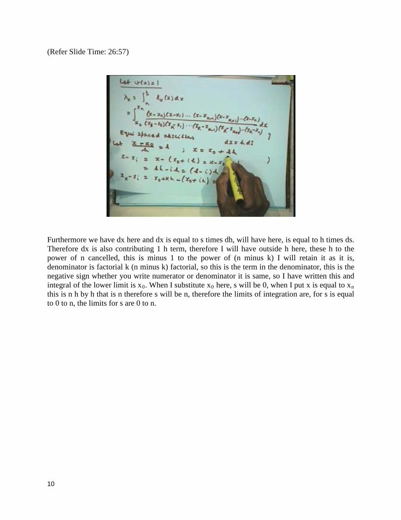
(Refer Slide Time: 26:57)
Furthermore we have dx here and dx is equal to s times dh, will have here, is equal to h times ds. Therefore dx is also contributing 1 h term, therefore I will have outside h here, these h to the power of n cancelled, this is minus 1 to the power of (n minus k) I will retain it as it is, denominator is factorial k (n minus k) factorial, so this is the term in the denominator, this is the negative sign whether you write numerator or denominator it is same, so I have written this and integral of the lower limit is x0. When I substitute x0 here, s will be 0, when I put x is equal to xn this is n h by h that is n therefore s will be n, therefore the limits of integration are, for s is equal to 0 to n, the limits for s are 0 to n.
10

(Refer Slide Time: 28:04)
And the integral is given by simply this quantity that is s into (s minus 1) so on (s minus k plus 1), (s minus k minus 1) so on (s minus 1) ds. Now we can also write down from here what will be the error term, the error term that we had written is this, so I can write down the error term from this using this, let us write error that is equal to Rn.
(Refer Slide Time: 28:40)
11

Now the numerator w(x) is 1 we have taken, pi(x) contains all the products, all the products means it will now contain the missing factor also that we have missed here (s minus k) so that missing factor will come here and hence it will be h to the power of n plus 1 and there is a h being contributed by dx, therefore we will have here h to the power of n plus 2, h to the power of n plus 1 contributed by this and dx is equal to h times ds. Denominator is the same that is your n plus 1 so we will have (n plus 1) factorial, integral of 0 to n and the s into (s minus 1), all the terms are here so simply (s minus 1) f(n+1) of zhi ds. This is the error term for the most general case and these lambdak’s are the weights in the integration formula and this entire set of formulas are called Newton-cotes formulas; they are called Newton-cotes formulas. If I take particular values of number of points n then I have various order formulas coming, let us first of all take a case n is equal to 1 which is a 2 point formula, this will be a 2 point formula. We are taking n plus 1 as the total number of points so if I take n is equal to 1, we are taking 2 point formula that is your x0 we are taking, f(x0) we are taking and (x1, f(x1)), these are the 2 points that we are taking. Therefore h will be simply equal to x1 minus x0 that is equal to simply b minus a. We are taking the entire interval a to b as only considering 2 points therefore it will be the upper limit and the lower limit therefore the distance between them will be your step length b minus a.
(Refer Slide Time: 31:12)
The formula will be integral of a to b f(x)dx, w is equal to 1 so f(x)dx is lambda0 f of x0 plus lambda1 f of x1, this is our formula of which x0 and x1 are fixed as a and b. Now lambda0 I can obtain from here, let us substitute k is equal to 0 in this to get our value, so I have to put n is equal to 1, k is equal to 0, I have to put here and k is equal to 0 and n is equal to 1. Therefore we will get lambda0 is equal to, n is 1, k is 0 so I will have a minus sign, minus h, this is factorial 0, factorial 1 so I will have denominator simply as 1. Integral of 0 to 1 that only n is equal to 1, 0 to 1 and the numerator should not contain x minus s k term that is your x minus x0 term that means
12

I should not have s in the integrant, so I will simply have s minus 1 ds. since we have taken only n is equal to 1 will have to consider only 2 terms of this, so of this lambda0 s will be missing, for lambda1 s minus 1 will be missing, so s missing so I will have simply this. Now I can integrate this and write this minus h s square by 2 that is half minus s that is 1, so that is equal to h upon 2. Now we have obtained already lambda0 so let us obtain lambda1.
(Refer Slide Time: 33:02)
So now I have to take n is equal to 1, k is equal to 1, I have to take n is equal to 1, k is equal to 1. So let us put in this n is equal to 1, k is equal to 1, therefore I will have lambda1, now n is 1, k is 1 so it will be positive sign and this is 1 factorial, this is 0 factorial so again I will have 1. 0 to 1 now s minus 1 will be missing so I will simply have s ds. Therefore this will give you h square by 2, s square by 2 therefore thats equal to n by 2. Therefore we have now derived the formula as integral a to b f(x)dx is equal to h by 2 [f of x0 plus f of x1]. If you want we can put it in terms of the upper and lower limit also, h is equal to b minus a so I can alternatively write this as (b minus a) by 2 [f(x0) plus f of x1] and again (b minus a) by 2 [f of a plus f of b]. So I can use this particular form or I can use this particular form for computation purposes. Now let us write down the error term, the error term is given by this, now n is equal to 1 therefore our error Rn is h cubed by factorial 2, I am putting n is equal to 1 here, 0 to 1 s into (s minus 1) f(n+1) zhi ds.
13

(Refer Slide Time: 35:07)
Now it is possible sometimes for us to use the mean value theorem of integral calculus to evaluate this as we have done earlier also. You can see that this product, this function s has got negative sign between 0 and 1 so it has the same sign, it has the same sign, minus sign in (0, 1). Therefore I can apply the mean value theorem where we have 0 to 1 sum f(x) g(x) dx is there, f(x) does not change its sign then g(x) can be taken out of the integral and evaluate it at any point in between 0 and 1. So apply the mean value theorem, use mean value theorem of integral calculus.
14

(Refer Slide Time: 36:04)
If I use this mean value theorem of integral calculus I can now take out this f(n+1) out and write this as h cubed by factorial 2, n is equal to 1 f double dashed of some eta, some other point some point in this one into integral 0 to 1, let us multiply it out s square minus s ds, where eta is lying between a and b, eta is lying between a and b. Now let us evaluate this, this is equal to h cubed by 2 f double dash of eta, this is x cubed by 3 that is [1 by 3 minus 1 by 2]. This gives you minus 1 by 6 so minus h cubed by 12 f double dash eta. If I want in terms of b minus a, I can also write in terms of (b minus a) whole cubed by 12 f double dash of eta. Now n is equal to 1 therefore as we are shown earlier this integral formula integrates exactly polynomials of degree less than or equal to 1, therefore this integrates polynomials of degree less than or equal to 1 that is all linear polynomials it will integrate exactly. Therefore integrates exactly polynomials of degree less than or equal to 1 that is because order is going to be n is equal to 1.
Indeed, of course we could have observed or derived this particular thing by looking at this error term. The error term consists of f double dash of eta, now if f is a linear polynomial it is second derivative is 0, therefore Rn is always going to be 0 whenever, whenever our f(x)is a linear polynomial. Therefore the conclusion that we have given here could be obtained by if you are able to derive the error formula, I can obtain the same observations from the error formula also. This formula is called the trapezoidal rule or trapezium rule, this is called the trapezium rule, trapezoidal or we can call it as trapezium rule.
15

(Refer Slide Time: 38:49)
If you are looking at integral a to b f(x) dx, why it is called a trapezium I am just trying to explain, if you are taking this is nothing but area under the curve from a to b f(x) so if I draw the graph of this, let us write a nice graph like this, let us take this as a, let us take this as b, then this is the graph of y is equal to f(x), this gives you area under the curve between the abscissa x is equal to a x is equal b and bounded by y is equal to f(x) above the x axis. Here what we are doing here is, we have written the formula as simply b minus a by 2 into f of a plus f of b that means what we have really done here is, we have now taken this as the approximate area, we have taken this as the approximate area by using this particular formula. This is nothing but the area of trapezium, now if you look at this trapezium this is nothing but the area of the trapezium, therefore it is called the trapezoidal rule or the trapezium rule. Now but the order of the formula is only one therefore it is very useful at the same time we would like to have better formulas.
16

(Refer Slide Time: 40:14)
So let us go for n is equal to 2 that is your 3 point formula that means we are using the 3 abscissas x0, x1, x2, they are equi distant therefore we are taking a, a plus b by 2 and b, these are 3 equi distant formulas therefore we have a, a plus b by 2 and b. Now I will have to substitute in this expression that we have derived earlier for lambdak for winding lambda0 I will have to substitute n is equal to 2, k is equal 0, integrate this I will have, then I will have 3 terms here s into (s minus 1) (s minus 2) one of them will be dropped for finding lambda0 that is s will be dropped, where I find s 1, lambda1, I will drop (s minus 1), when I find lambda2 I drop (s minus 2). So it is simply integration of this between the limits 0 to 2; I have to integrate between 0 to 2. Now I will give the values for the lambdas that is very simple straight forward to be can be obtained that is h upon 3, lambda1 is equal to 4 h by 3 and lambda2 is equal to h by 3. h of course is the distance between x1 and x0 and this, therefore your h is equal to x1 minus x0 or same as x2 minus x1 therefore this will be b minus a by 2. This is the 3 point so it will be 2 intervals because the 2 intervals we are taking, the 2 intervals are x0, x1, x1, x2, therefore the step length that we have will be, having will b minus a by 2, so that it is divided into 3 equi distant points.
Therefore the formula would be integral a to b f(x) dx is equal to h by 3 [f of x0 4 times f of x1 plus f of x2]. If I write in terms of the n points, upper and lower limits I can write down b minus a, this is 2 therefore I have a 6 here, [f of a 4 times f of (a plus b by 2) plus f of b]. Now let us write down the error also from here, error formula can immediately be written down but the error formula as given is difficult for me so what I would do is I will write the alternative form of the error that is given to us. We have written the error constant, we have defined the error constant, I would like to use this to derive the error formula for this formula. Now n is equal to 2 therefore it should integrate polynomials of degree less than or equal to 2 so let us first say integrates
17

polynomials of degree less than or equal to 2. Therefore our error term should come from the next power of x that is x cubed, this is n is equal to 2 therefore I must use x to the power of n plus 1 that is 3 and that should give me the error constant therefore let us write down the error constant.
(Refer Slide Time: 43:52)
The error constant c would be equal to integral of a to b, integral of a to b x cubed dx minus lambda0 f(x0), we will write down this expression but just write down the original formula. Now let us put the value of this, this is equal to integral a to b, let us integrate this x4 by 4 so I will have 1 by 4 (b to the power of 4 minus a to the power of 4) minus this is b minus a by 6, I am writing from here, I am writing from this formula. This is your f of a, I will substitute for x in a moment but let us just write down the formula, this is 4 times f of (a plus b by 2) plus f of b. So let us put the value of f, f is x cubed therefore this is 1 upon 4 (b to the power of 4 minus a to the power of 4)( b minus a) by 6, f is x cubed therefore this is a cubed plus 4 upon 8 (a plus b) whole cubed plus b cubed.
Now I will leave this as a simple exercise for you to just open it up and show that it turns out to be 0. Just multiply it out everything cancels and we will have only b4 minus a4 here and we will get this is equal to 0. Therefore the error constant has turned out to be 0, before we had written this we said it integrates polynomials of degree less than or equal to 2 but now error constant has become 0, so it is integrating x cubed also exactly, therefore this formula is integrating polynomials of degree less than or equal to 3 exactly. Therefore we conclude from here immediately integrates polynomials of degree less than or equal to 3 exactly, it is not 2 but 3 therefore the order of this formula is now 3.
18

(Refer Slide Time: 46:39)
Now I want the constant c therefore I must go to the next term that is I have to go to a to b x to the power of 4 dx that is a next value of x, that is x to the power of 4 dx minus (b minus a) by 6 f of a that is a to the power of 4 upon 16 (a plus b) to the power of 4 plus b to the power of 4, f of a f of a, a plus b by 2 and f of b. Now I can integrate this, this will give you minus 1 upon 5 x to the power of 5 by 5 that is b 5 minus a 5 and this. Now I will leave this also an exercise for you, it comes out to be very simple expression as (b minus a) to the power of 5 by 120. This combines with this and they would all become a perfect factor and it would become (b minus a) to the power of 5 by 120. Therefore our error is not R2 but R3, n is now instead of 2 it has become 3, so R3 is equal to c upon, if you had written the previous one it will be factorial 3, now c was 0 so I will have factorial 4 f fourth derivative eta. Now this also would now tell us that is the fourth derivative occurring for 5 f therefore integrates exactly all polynomials of degree less than or equal to 3. Therefore we are proving from here also that it is a order 3.
Now I substitute this therefore I will have b minus a by 5 24 into 120 f iv eta. Now this form I can use alternatively, I would like to use the form of the step length h, the step length h for this was, h was b minus a by 2 therefore I can use b minus a is 2 h, therefore b minus a to the power of 5 will be 2 to the power of 5 32 h to the power of 5 by 24 into 120 f4 eta. This is 28, 80 and 32 cancels off, it becomes 90 so I will have here h5 by 90, f iv of eta. Now this clause of formulas is called the Simpson’s integration formulas, these are the Simpson rules. Some books call it as one third rule but whenever we talk of Simpson’s rule we always mean this particular rule and this is a formula which has got precision or order 3 and the error term is quite small that is h to the power of 5 by 90 fourth derivative of this. When f(x) is a continuous function that is given to us
19

fiv is bounded. Therefore the error is now really governed by this particular factor that we have over here and we can see by improving by one point the order has jumped also and also it has become very very accurate it is going to be. Okay would stop with this.
20


