Numerical Simulation of Turbulent Free-Surface Flow

in Curved Channel∗

T. Bodnar and J. PrıhodaInstitute of Thermomechanics, Academy of Sciences of Czech Republic

Abstract. This paper presents first results of numerical simulation of turbulentfree-surface flow. Simple implementation of surface capturing method is based onthe variable density approach. The flow is treated as if there is only one fluid, butwith variable material properties (density, viscosity). The switch in these values isdone by a function resulting from the mass conservation principle. This approachsimplifies the implementation of turbulence model. In this case the SST k−ω modelwas chosen in modification given by Hellsten.

Numerical solution was carried out by finite-volume method with explicit Runge-Kutta time-integration. The artificial compressibility method was used for time-marching search for steady state solution. The whole model was tested on hori-zontally placed square-sectioned 90 bend, which was partially filled by the water.The main goal of this study was to demonstrate the applicability of this model andsolution method for capturing the water-air interface as well as for predicting theturbulent effects in both fluids.

Keywords: turbulent flow, free-surface, finite volume, artificial compressibility

1. Introduction

Numerical simulation of free-surface flows is one of the most compli-cated tasks of CFD. There are two main groups of methods applied tothe free-surface resolution.

Interface tracking methods define the free-surface as a sharp interfacewhose motion is followed. The interface forms a part of the computa-tional domain boundary and thus the mesh must be readjusted as thefree-surface evolves. Interface capturing methods work on fixed grid,which extends beyond the free-surface. The shape of the free-surface isdetermined by cells which are partially filled.

In general, interface tracking methods are more accurate than in-terface capturing methods and more efficient for very simple physicalsituations. However, the interface tracking methods are usually limitedonly to these very simple situations. With the increasing need to solvevery complex cases, the necessity of use of interface capturing methodshas arrised.

∗ This work was supported by the Research Plan No. AV0Z20760514 of theAcademy of Sciences of Czech Republic

c© 2005 Kluwer Academic Publishers. Printed in the Netherlands.

paper_01.tex; 24/06/2005; 10:01; p.1

2

Therefore the method we have used in our study is based on oneof the possible implementations of interface capturing methods. Thecase solved here is the flow in a square sectioned 90 bend, which ispartially filled by the water. Because of the action of the centrifugalforce, the water-air interface is deformed in the bend. The shape ofthe free-surface is relatively simple in this case, however its correctresolution at high Reynolds number in a fully turbulent flow is a verycomplicated task.

2. Mathematical Model

The approach used in our model is based on the assumptions for variable-density incompressible flow. It means the flow is treated as if the domainis filled by only one fluid, which density is variable. The discontinuity indensity profile arises at the free-surface. The key point in the modellingof this kind of flows is the appropriate formulation of mass conservationlaw, i.e. in the choice of adequate form of continuity equation. In thiscase the full ”compressible” version should be used.

2.1. Mass conservation

∂ρ

∂t+ div (ρv) = 0 (1)

Using the chain rule, this could be rewritten as:

∂ρ

∂t+ v · grad ρ = −ρ divv (2)

Because of the incompressibility assumption, the right-hand side ofequation (2) should be equal zero. From this directly follows the ex-pression on the left-hand side is then also equal zero. This means thatthe mass conservation in variable-density incompressible flows requirestwo separate conditions to be fullfiled:

a) Density transport equation

∂ρ

∂t+ v · grad ρ = 0 (3)

b) Divergence-free constrain

divv = 0 (4)

paper_01.tex; 24/06/2005; 10:01; p.2

3

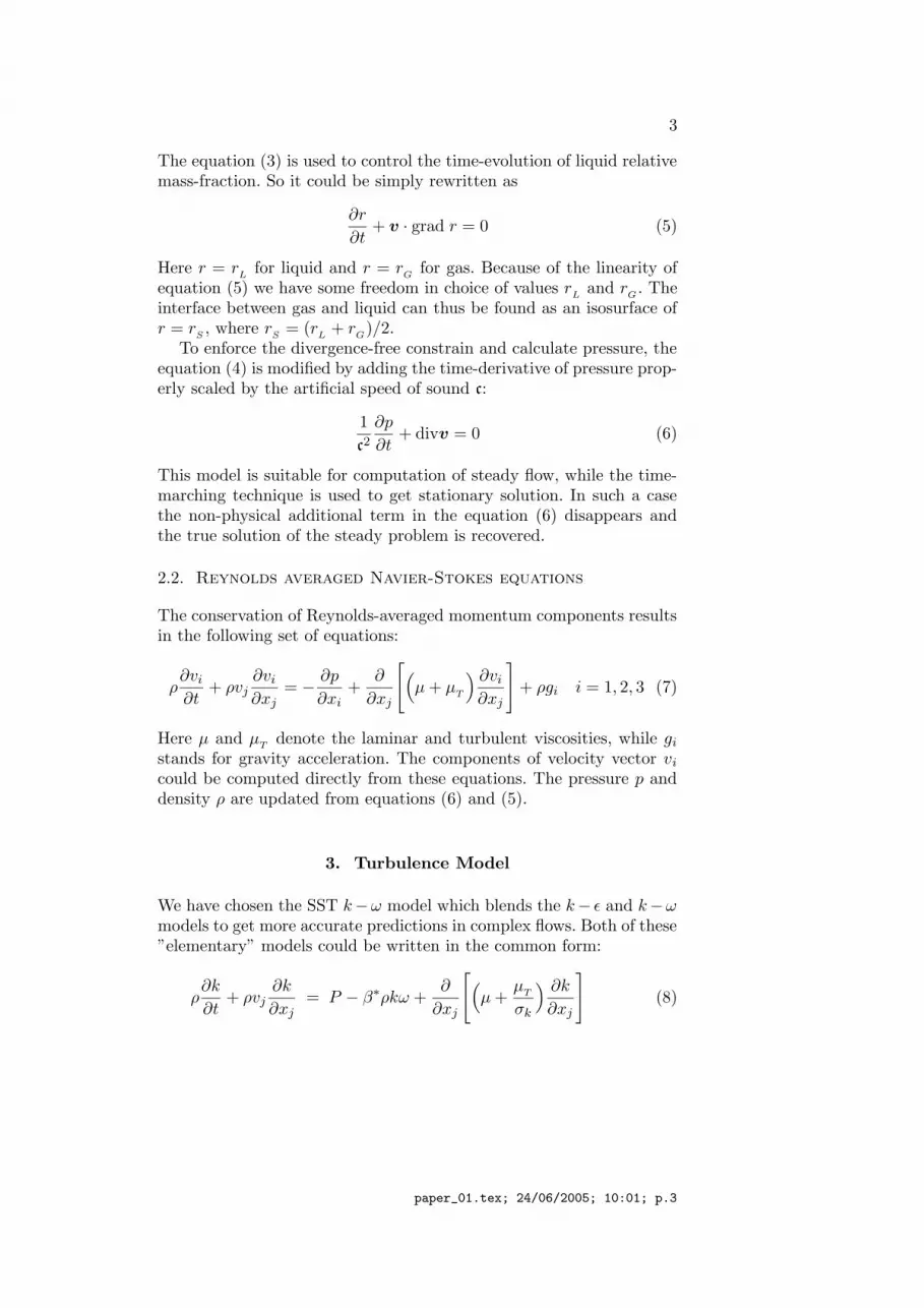
The equation (3) is used to control the time-evolution of liquid relativemass-fraction. So it could be simply rewritten as

∂r

∂t+ v · grad r = 0 (5)

Here r = rL

for liquid and r = rG

for gas. Because of the linearity ofequation (5) we have some freedom in choice of values r

Land r

G. The

interface between gas and liquid can thus be found as an isosurface ofr = r

S, where r

S= (r

L+ r

G)/2.

To enforce the divergence-free constrain and calculate pressure, theequation (4) is modified by adding the time-derivative of pressure prop-erly scaled by the artificial speed of sound c:

1

c2

∂p

∂t+ divv = 0 (6)

This model is suitable for computation of steady flow, while the time-marching technique is used to get stationary solution. In such a casethe non-physical additional term in the equation (6) disappears andthe true solution of the steady problem is recovered.

2.2. Reynolds averaged Navier-Stokes equations

The conservation of Reynolds-averaged momentum components resultsin the following set of equations:

ρ∂vi

∂t+ ρvj

∂vi

∂xj= − ∂p

∂xi+

∂

∂xj

[

(

µ + µT

) ∂vi

∂xj

]

+ ρgi i = 1, 2, 3 (7)

Here µ and µT

denote the laminar and turbulent viscosities, while gi

stands for gravity acceleration. The components of velocity vector vi

could be computed directly from these equations. The pressure p anddensity ρ are updated from equations (6) and (5).

3. Turbulence Model

We have chosen the SST k−ω model which blends the k− ε and k−ωmodels to get more accurate predictions in complex flows. Both of these”elementary” models could be written in the common form:

ρ∂k

∂t+ ρvj

∂k

∂xj= P − β∗ρkω +

∂

∂xj

[

(

µ +µ

T

σk

) ∂k

∂xj

]

(8)

paper_01.tex; 24/06/2005; 10:01; p.3

4

ρ∂ω

∂t+ ρvj

∂ω

∂xj=

γρ

µT

P − F4βρω2 +∂

∂xj

[

(

µ +µ

T

σω

) ∂ω

∂xj

]

+ 2ρ1 − F1

σω2ω

∂k

∂xj

∂ω

∂xj(9)

Model costants are slightly different for each of these models. Theblending between k−ω and k−ε model is provided by switching betweentheir parameters .

σk

σω

β

= F1

σk1

σω1

β1

+ (1 − F1)

σk2

σω2

β2

(10)

Here the blending function F1 reads:

F1 = tanh(Γ4) with Γ = min

[

max(

√k

β∗ωd;500ν

ωd2

)

;4ρσω2k

CDkωd2

]

(11)

The CDkω stands for positive part of cross-diffusion term

CDkω = max

[

2ρ

σω2ω

∂k

∂xj

∂ω

∂xj; CDkω min

]

(12)

The cross-diffusion minimum value should be prescribed (i.e. CDkω min =10−10).Model constants for k − ω model are:

σk1 = 2.0 σω1 = 2.0 β1 = 0.075 (13)

Model constants for k − ε model:

σk2 = 1.0 σω2 = 1.168 β2 = 0.0828 (14)

Further parameters: κ = 0.41 and β∗ = 0.09. Parameter γ is computedfrom:

γ =β

β∗− σωκ2

√β∗

(15)

Turbulent kinetic energy production is given by

P =(

2µTSij −

2

3δijρk

) ∂vi

∂xj(16)

The symmetric part of the velocity gradient is defined as follows:

Sij =1

2

( ∂vi

∂xj+

∂vj

∂xi

)

with norm |Sij | =√

2SijSij (17)

paper_01.tex; 24/06/2005; 10:01; p.4

5

The turbulent viscosity is evaluated from

µT

=a1ρk

max(a1ω; |Sij |F2F3)where a1 = 0.31 (18)

The function F2 is evaluated from:

F2 = tanh(Γ22) with Γ2 = max

( 2√

k

β∗ωd;500ν

ωd2

)

(19)

The function F3 is given by:

F3 = 1 − tanh

[

(

150ν

ωd2

)4]

(20)

The streamline curvature effect is taken into account by the functionF4, given by the following formula:

F4 =1

1 + CrcRiwhere Crc ≈ 3.6 (21)

The Richardson number Ri is defined by:

Ri =|Ωij ||Sij |

( |Ωij ||Sij |

− 1

)

(22)

Here the anti-symmetric part of the velocity gradient is defined asfollows:

Ωij =1

2

( ∂vi

∂xj− ∂vj

∂xi

)

with norm |Ωij | =√

2ΩijΩij (23)

Boundary conditions

The boundary conditions for the presented model were chosen accord-ing to the original paper (Hellsten, 1998). The model allows to setboundary conditions on inpermeable wall depending on the surfaceroughness.

Rough wall

ω =u2

τ

νS

Rwhere the friction velocity uτ =

√

τw/ρ (24)

The nondimensional function SR

is given by

SR

=

(

50max(k+

s ;k+smin)

)2for k+

s < 25

100k+

s

for k+s ≥ 25

(25)

paper_01.tex; 24/06/2005; 10:01; p.5

6

In the above equations the nondimensional sand-grain height is:

k+s =

uτks

ν(26)

Its minimal value could be evaluated from

k+smin = 2.4 (y+

1 )0.85 where y+1 =

uτ∆d1

ν(27)

In our case the wall was assumed to be idealy smooth, so the valuek+

s = k+smin was used on the wall.

Free stream

The following free stream values for k, ω, and νT

could be used

ω∞ = C · V∞/L (28)

νT∞ = 10−3ν (29)

k∞ = νT∞ ω∞ (30)

Here C ≈ 1 ÷ 10 and L is the characteristic scale of the flow.

4. Numerical Solution

Numerical solution of the above presented mathematical model is basedon finite-volume cell-centered semi-discretization on structured mesh.The time-integration of the resulting system of ordinary differentialequations is carried out using explicit Runge-Kutta multistage scheme.Because of the use of the central-differencing in spatial discretization,suitable stabilization technique is used to avoid non-physical oscilla-tions in the solution.

4.1. Space Discretization

The computational mesh is structured, consisting of hexahedral pri-mary control volumes. To evaluate the viscous fluxes also dual finitevolumes are needed. These have octahedral shape and are centeredaround the corresponding primary cell faces. See the following figure 1for the schematic view of such configuration.

paper_01.tex; 24/06/2005; 10:01; p.6

7

Figure 1. Finite-volume grid in 3D

The system of RANS equations (including the modified continuityequation) could be rewritten in the vector form. Here we use W todenote the vector of unknowns (including pressure). Vectors F, G and H

denote the inviscid fluxes in x,y,z directions, while R, S and T stand fortheir viscous counterparts. Using this notation, the spatial finite-volumesemi-discretization could be written in the following form:

∂Wijk

∂t= − 1

|D|

∮

∂D

[

(F−R), (G− S), (H−T)]

· ν dS +1

|D|

∫

D

fW

(31)

Here D denotes the computational cell, ν is the outer unit normalvector of the cell boundary, dS is the surface element of this boundary.The vector f

Wcontains the external body forces (e.g. gravity in our

case). The equation (31) can be rewritten in operator form:

∂Wijk

∂t= −LWi,j,k (32)

Here L stands for the finite-volume discretization operator. This oper-ator is still exact at this stage and it should be properly discretized toallow for numerical solution. This is done by the replacement of fluxesin it’s formulation by their numerical (approximate) versions.

The inviscid flux integral can be approximated in a central manner,e.g. the value of the flux F on the cell face with index ` = 1 is computedas average of cell-centered values from both sides of this face:

paper_01.tex; 24/06/2005; 10:01; p.7

8

Di,j,ki+1,j,kD

l=1

Figure 2. Inviscid flux discretization

Fn1 =

1

2[F(Wn

i,j,k) + F(Wni+1,j,k)] (33)

The contribution of inviscid fluxes is finally summed up over the cellfaces ` = 1, . . . , 6. In this way we can write down the inviscid fluxapproximation:

∮

∂D

Fνx dy dz ≈6∑

`=1

F`νx` S` (34)

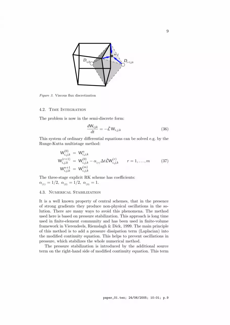
The discretization of viscous fluxes is a little bit more complicatedbecause the vectors R, S, T were defined using the derivatives of velocitycomponents. So we need to approximate somehow these derivatives atcell faces. This can be done using the dual finite-volume grid that iscentered around the corresponding faces (see Figure 1 and 3).

The evaluation of velocity gradient components is then replaced bythe surface integral over the dual volume boundary. Finally this surfaceintegral is approximated by a discrete sum over the dual cell faces(with indices m = 1, . . . , 8). For example trying to evaluate the firstcomponent of the viscous flux R1 (i.e. approximate ux) at the cell facel = 1 we must proceed in the following way:

ux ≈∮

∂D

u νx dy dz ≈8∑

m=1

umνxmSm (35)

The outer normal of the dual cell faces should be properly approximatedνx ≈ νx

m. The values of velocity components in the middle nodes ofthese faces are taken as an average of the values in the correspondingvertices.

paper_01.tex; 24/06/2005; 10:01; p.8

9

Di+1,j,ki,j,kD

m=1

Figure 3. Viscous flux discretization

4.2. Time Integration

The problem is now in the semi-discrete form:

dWijk

dt= −LWi,j,k (36)

This system of ordinary differential equations can be solved e.g. by theRunge-Kutta multistage method:

W(0)i,j,k = W

ni,j,k

W(r+1)i,j,k = W

(0)i,j,k − α

(r)∆tLW

(r)i,j,k r = 1, . . . , m (37)

Wn+1i,j,k = W

(m)i,j,k

The three-stage explicit RK scheme has coefficients:α

(1)= 1/2, α

(2)= 1/2, α

(3)= 1.

4.3. Numerical Stabilization

It is a well known property of central schemes, that in the presenceof strong gradients they produce non-physical oscillations in the so-lution. There are many ways to avoid this phenomena. The methodused here is based on pressure stabilization. This approach is long timeused in finite-element community and has been used in finite-volumeframework in Vierendeels, Riemslagh & Dick, 1999. The main principleof this method is to add a pressure dissipation term (Laplacian) intothe modified continuity equation. This helps to prevent oscillations inpressure, which stabilizes the whole numerical method.

The pressure stabilization is introduced by the additional sourceterm on the right-hand side of modified continuity equation. This term

paper_01.tex; 24/06/2005; 10:01; p.9

10

has the following form:

Qi,j,k =1

|Di,j,k|

2N∑

`=1

p` − pi,j,k

b`

S` (38)

Here ` denotes the control volume cell face index, p` is the pressurein the corresponding neighboring cell and S` is the cell face area. Thevalue bell has the dimension of velocity and represents the maximalconvective velocity in the domain and local diffusive velocity.

b` = max(√

v21 + v2

2 + v23) +

2ν

L`

(39)

Symbol L` corresponds to a distance between the actual and neighbor-ing cell centers.

It is possible to show, that on the uniform cartesian mesh with cellsof size δx this term gives:

Q =δx

2b∆p (40)

This type of numerical stabilization has some advantages over theclassical artificial diffusion applied to the velocity components. First,its ”artificial” effects are clearly separated from the physical viscosityincluded in RANS equations. Even more important property of thisstabilization term is that it contains only second derivatives of pressureand thus it will vanish if pressure will be a linear function of spacecoordinates. This is the case of e.g. Poiseuille flow with linear pressuredecay along the flow axis. Also the pressure being constant across theboundary layer, forces the stabilizing source term to disappear fromcontinuity equation.

5. Numerical Results

Numerical tests were performed for thecurved channel with squarecross-section. The 90 bend was oriented with the plane of symmetryin horizontal position. Channel is partially filled by the water (up tothe symmetry plane), while the remaining volume is occupied by air.Uniform velocity 1 m/s was assumed for both fluids on the inlet. Thenumerical results presented here were chosen to show the resolution ofthe free-surface in the bend.

paper_01.tex; 24/06/2005; 10:01; p.10

11

X Y

Z

a

a

Figure 4. Free-surface in 3D view

Z

X

Y

Figure 5. Free-surface in 3D view

The lengths of inflow and outflow parts of the channel were chosenvery short to decrease the overall computational time. These partshowever should be significantly longer for real configurations to avoidnon-physical boundary effects in the proximity of the bend .

The Figure 6 shows the 3D view of the water-air interface. Thecontours of the surface elevation are drawn in the same figure. Thesecontours are shown separately in 2D view in the Figure 7.

X

ZY

Figure 6. Free-surface in 3D view

X

Z

Y

Figure 7. Free-surface elevation contours

The position of the free-surface and its spatial evolution in thestream-wise direction from the inlet can be seen in the Figure 8 and 9in detail.

paper_01.tex; 24/06/2005; 10:01; p.11

12

X Y

Z

Inlet

0

30

60 90

-0.1 -0.05 0 0.05 0.1R-a

-0.1

-0.05

0

0.05

0.1

030

6090

y

Figure 8. Free-surface elevation at different sections

In the Figure 8 is visible also the near-wall shape of the free surface.This, a litle bit unexpected profiles are probably caused by the absenceof surface tension in our model. This phenomena however could playimportant role in real case and its effectl should be introduced into ourmodel in the future.

The traces of water-air interface on channel side-walls and in theaxial plane are shown in Figure 9:

Axial position

-0.1

-0.05

0

0.05

0.1

00 30 60 90Inlet Outlet

y

Outer Wall

Inner Wall

Axial Plane

Figure 9. Longitudinal free surface profiles

These profiles are close to what was expected. The only issue to beaddressed in this case is a small ”wave” close to the inlet section. This isnot physical and it is caused by the presence of artificial inlet boundary,

paper_01.tex; 24/06/2005; 10:01; p.12

13

where the uniform velocity profile was prescribed. The fast change inthe velocity profile introduces an impuls to a free surface to form sucha wave. This could be handled by shifting the inlet boundary furtherfrom the bend and mainly by prescription of some more realistic, fullydeveloped velocity profile.

The last set of pictures in Figure 10 shows the turbulent kineticenergy contours for selected sections within the bend.

-0.1

-0.05

0

0.05

0.1

-0.1 -0.05 0 0.05 0.1R-a

y

-0.1

-0.05

0

0.05

0.1

-0.1 -0.05 0 0.05 0.1R-a

y

a. 0 section b. 30 section

-0.1

-0.05

0

0.05

0.1

-0.1 -0.05 0 0.05 0.1R-a

y

-0.1

-0.05

0

0.05

0.1

-0.1 -0.05 0 0.05 0.1R-a

y

c. 60 section d. 90 section

Figure 10. Turbulent kinetic energy isolines at different sections

These contours show the very thin TKE boundary layer in both,water and air. However the maximum appears in the region, where thefree surface minima takes a place. This is the mst kritical region wherethe velocity changes very quickly in magnitude and direction.

6. Conclusions & Remarks

The range of numerical test we have performed for the selected flowsetup has shown the possibility to model turbulent free-surface flows

paper_01.tex; 24/06/2005; 10:01; p.13

14

by the presented ”variable density” approach. The straightforward for-mulation and use of the mass conservation principle for capturing thefree-surface allows us to distinguish between cells occupied by waterand by the air. The use of the turbulence model is than reduced to itsimplementation for the two-component fluid mixture with mixing ratiogiven point-wise by the density transport equation.

The model predictions for both free-surface position and turbulentquantities seem to be qualitatively correct. Actually it was not possibleto validate the code on experimental data because of the absence ofsuitable data set providing sufficient free-surface and turbulence infor-mation for one experiment. This is one of the essential tasks for themodel evolution and practical use.

There are still several issues connected with this approach thatshould be addressed in future work. They are however rather connectedwith numerical issues than with the model itself. Both time- and spacediscretization should be further refined to get higher overall efficiencyand robustness.

References

Benes, L. & Kozel, K.: Numerical Simulation of 3D Atmospheric Boundary LayerFlow with Pollution Dispersion. In: Proceedings of International Conference onAdvanced Engineering Design, (pp. 141–146). University of Glasgow, Glasgow(2001). ISBN 0-85261-731-3.

Ferziger, J. H. & Peric, M.: Computational Methods for Fluid Dynamics. SpringerVerlag (1997).

Hellsten, A.: Some improvements in Menter’s k − ω SST turbulence model. Tech.rep., American Institute of Aeronautics and Astronautics (1998). AIAA-98-2554.

Ransau, S. R.: Solution Methods for Incompressible Viscous Free Surface Flows: ALiterature Review. Preprint 3/2002, Norwegian University of Science and Tech-nology, Department of Mathematical Sciences, Norvegian University of Scienceand Technology, N-7491 Trondheim, Norway (2002).

Vierendeels,J. , Riemslagh, K. and Dick, E.: A Multigrid Semi-implicit Line-Methodfor Viscous Incompressible and Low-Mach-Number Flows on High Aspect RatioGrids Journal of Computational Physics 154, pp. 310–341 (1999)

paper_01.tex; 24/06/2005; 10:01; p.14