Numerical Simulations of Unsteady Shock WaveInteractions Using SaC and Fortran-90

Daniel Rolls2, Carl Joslin2, Alexei Kudryavtsev1, Sven-Bodo Scholz2, and AlexShafarenko2

1 Institute of Theoretical and Applied Mechanics RAS SB,Institutskaya st. 4/5,

Novosibirsk, 630090, Russia2 Department of Computer Science, University of Hertfordshire, AL10 9AB, UK

Abstract. This paper briefly introduces SaC: a data-parallel languagewith an imperative feel but side-effect free and declarative. The expe-riences of porting a simulation of unsteady shock waves in the Eulersystem from Fortran to SaC are reported. Both the SaC and Fortrancode was run on a 16-core AMD machine. We demonstrate scalabilityand performance of our approach by comparison to Fortran.

1 Introduction

In the past when high performance was desired from code, high-levels of ab-straction had to be comprimised. This paper will demonstrate our approachwhich overcomes these shortcomings: we will present the data-parallel languageSaC [1] and exemplify its usage by implementing an unsteady shock wave sim-ulator in the Euler system. SaC was developed by an international consortiumcoordinated by one of the authors (Sven-Bodo Scholz). We will compare theperformance of our approach against Fortran by running this application on a16-core computation server.

The language is close to C syntactically, which makes it more accessible tocomputational scientists, while at the same time being a side-effect free, declar-ative language. The latter enables a whole host of intricate optimisations in thecompiler and, perhaps more importantly, liberates the programmer from imple-mentation concerns, such as the efficiency of memory access and space manage-ment, exploitation of data-parallelism and optimisation of iteration spaces. Inaddition, code that was written for a specific dimensionality of arrays can bereused in higher dimensions thanks to an elaborate system of array subtypingin SaC, as well as its facilities for function and operator overloading that farexceed the capabilities of not only Fortran but the object-orientation languagesas well.

SaC has already been used for many kinds of application, ranging fromimage-processing to cryptography to signal analysis. However, to our knowl-edge there has been only one occasion of programming a Computational FluidDymamics application in SaC namely the Kademtsev-Petviashivili system [2].

Even that example is too esoteric to support any conclusions about practicalsuitability of Single-Assignment C. In this paper we present for the first timethe results of using SaC as a tool in solving a real, practical problem: simulationof unsteady shock waves in the Euler system.

The equations of fluid mechanics can be solved analitically for only a limitednumber of simple flows. As a consequence, numerical simulation of fluid flowsknown as Computational Fluid Dynamics (CFD) is widely used in both scientificresearch and countless engineering applications. Efficiency of computations andease of code development is of great importance in CFD which is one of the mostperspective fields for implementing new concepts and tools of computer science.

In Section 2 we will briefly outline the features of SaC that we would arguemake it uniquely suitable for the class of applications being discussed. Section 3delineates the numerical method being used and Section 4 discuses implemen-tation issues we came across when porting a Fortran TVD implementatin toSaC. Our results are then presented in Section 5 and related work is discussedin Section 6 before finally Section 7 discusses the lessons learnt and concludes.

2 SaC

SaC is an array processing language that first appears to be an imperitive pro-gram like Fortran but actually has more in common with functional programminglanguages. A SaC function consists of a sequence of statements that define andre-define array objects. To a C programmer this looks very similar to assigningthe result of expressions to arrays, but there is an important difference: whatmay appear to the programmer to be the “control flow” in SaC is in fact a chainof definitions that link with one another via the use of common variables, thisemphasises data as opposed to control dependencies. Thus any iterative updatebecomes essentially a recurrence relation between the snapshots of the arraysbeing updated, and it is up to the compiler whether or not the arrays need tobe recreated as objects in memory or whether the underlying computation maybe taken in-flow. That not withstanding, analogues of control structures, suchas the IF statement, are provided, if only with a slightly different interpretation,so the illusion of programming a control flow may be retained as far as possible.

Two main constructs of SaC support the kind of computation that we areconcerned with in this paper:

Most of the high level constructions in this paper are compiled down to thefollowing to constructs.

with-loop Despite the name, which reflects some historic choices of terminol-ogy in SaC, the essence of this construct is a data-parallel array definition.The programmer supplies a specification of the index space (in an extendedenumeration form) and the definition of the array value for a given index interms of an expression with other values possibly indexed and produced byexternal functions. Definitions for different array values are assumed to bemutually independent, hence data-parallelism is presented to the compilerexplicitly.

for loop This is used for programming recurrences. The recurrence index isspecified in the for loop together with its initial value and increment, thecompiler interprets the loop body as a definition of the arrays emerging atthe final step of the recurrence in terms of the arrays defined prior to thefirst step.

As with FORTRAN-90 small arithmetic expressions in SaC can operate onwhole arrays to conveniently express elementwise operations on those arrays.E.g. a - b * c + c could be both an expression operating on scalars, arraysor scalars and arrays where the scalar form of the expression is applied to cor-responding indicies in the arrays a, b and c. For consise expressivness SaCsupports set notation which allows an expression to be defined for every el-ement of a new array where each expression may depend on the index. E.g.{ [i,j] -> matrix[j,i] } transposes a matrix by placing element (j, i) fromthe original matrix into element (i, j) for all i and j.

Another feature of the language that finds its use in the application beingreported is its type system, which supports subtyping. To provide an overviewof this, we remark, by way of an example, that a vector can be interpretedas a two dimensional array obtained by replicating the vector as a row in thecolumn dimension. This is a subtype of a general two dimensional array type. Oneconsequence of this is that a function that contains a tridiagonal solver for a one-dimensional Poisson equation can be applied to a two dimensional array (actingrow-wise) and then applied again column-wise by using two transpositions, allwithout changing a single line of code in the solver definition.

All these features make it possible to write function bodies that act on inputsof any dimension which suffer no performance loss compared to more specializedfunction bodies. Our code makes use of this fact to reuse function bodies for aone dimensional and two dimensional shockwave simulation.

3 Application

SaC is used to develop an efficient solver for the compressible Euler equations,which govern the flow of an inviscid perfect gas:

∂Q∂t

+∂F∂x

+∂G∂y

= 0, (1)

Q =

ρρuρvE

, F =

ρuρu2

ρuvu(E + p)

, G =

ρvρuvρv2

v(E + p)

. (2)

Here t is time, x and y are spatial coordinates, u and v are components ofthe flow velocity, ρ is density, p is the pressure related to the total energy E as

p = (γ − 1)(E − ρ

u2 + v2

2

), (3)

where γ is the ratio of specific heats (γ = 1.4 for air). The Euler equationsare the canonical example of a hyperbolic system of nonlinear conservation lawsthat describe conservation of mass, momentum and energy. Numerical methods,originally developed for the Euler equations, can be also used for a wide varietyof other hyperbolic systems of conservation laws, which arise in physical modelsdescribing physical phenomena in fields as varied as acoustics and gas dynamics,traffic flow, elasticity, astrophysics and cosmology. Thus, the Euler solver is arepresentative example of a broad class of computational physics programs.

A salient feature of nonlinear hyperbolic equations is the emergence of dis-continuous solutions such as shock waves, fluid and material interfaces. It turnstheir numerical solution into a non-trivial task. Modern numerical methods forsolving the hyperbolic equation [3] are based on high-resolution shock-capturingschemes originated from the seminal Godunov’s paper [4]. In these methods, thecomputational domain is divided into a number of grid cells and the conserva-tion laws are written for each cell. The computational procedure includes threestages: 1) reconstruction (in each cell) of the flow variables on the cell faces fromcell-averaged variables; 2) evaluation of the numerical fluxes through the cellboundaries; and 3) advancement of the solution from the time tn to time tn+1

where tn+1 = tn + ∆t. These stages are successively reiterated during the timeintergation of Eq (1).

The reconstruction during the first stage should avoid the interpolation acrossthe flow discontinuities. Otherwise, numerical simulations fail because of a lossof monotonicity and numerical oscillations developing near the discontinuities.The Fortran code developed includes several techniques of monotone reconstruc-tion, in particular, the TVD (Total Variation Diminishing) reconstructions ofthe 2nd and 3rd orders with various slope limiters and the 3rd order WENO(Weighted Essentially Non-Oscillatory) reconstruction, which automatically as-signs the zero weight to the stencils crossing a discontinuity. The latter techniqueis used in the examples of flow computation below. The reconstruction is appliedto the so-called (local) characterisic variables rather than to the primitive vari-ables ρ, u, v and p or the conservative variables Q.

The evaluation of numerical axes is performed by approximately solving theRiemann problems between two states on the “left” and “right” sides of the cellboundaries resulting from the reconstruction. The code includes a few optionsfor the approximate Riemann solver, below the results obtained from the shockwave simulation are presented. For time advancement (Stage 3) the 2nd or 3rdorder TVD Runge-Kutta schemes are used.

As an example of flow computations both a one dimensional and two dimen-sional problem is described below.

3.1 One Dimensional Simulation

The Euler code was used to solve the Sod shock tube problem [5], a commontest for the accuracy of computational gasdynamics code. The test consists ofa one dimensional Riemann problem. At the initial moment, the diaphragmseparates two resting gases with different pressures and densities. The top state

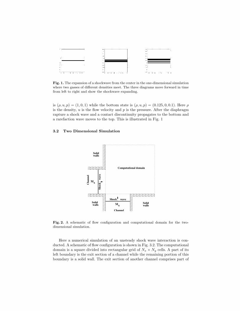
Fig. 1. The expansion of a shockwave from the center in the one-dimensional simulationwhere two gasses of different densities meet. The three diagrams move forward in timefrom left to right and show the shockwave expanding.

is (ρ, u, p) = (1, 0, 1) while the bottom state is (ρ, u, p) = (0.125, 0, 0.1). Here ρis the density, u is the flow velocity and p is the pressure. After the diaphragmrapture a shock wave and a contact discontinuity propagates to the bottom anda rarefaction wave moves to the top. This is illustrated in Fig. 1

3.2 Two Dimensional Simulation

���������������������������������������������������������������������������������������������������������������������������������������������������������������������������������������������������������������������������������

���������������������������������������������������������������������������������������������������������������������������������������������������������������������������������������������������������������������������������

������������������������������������������������������������������������������������������������������������������������������������������������������������������

������������������������������������������������������������������������������������������������������������������������������������������������������������������

������������������������������������������������������������������������������������������������������������������������������������������������������������������������������������������������������������������������������������������

������������������������������������������������������������������������������������������������������������������������������������������������������������������������������������������������������������������������������������������

Ms

Ms

Computational domain

Ch

an

nel

Channel

Shock wave

Sh

ock

wa

ve

Solidwalls

Solidwalls

Solidwalls

Fig. 2. A schematic of flow configuration and computational domain for the two-dimensional simulation.

Here a numerical simulation of an unsteady shock wave interaction is con-ducted. A schematic of flow configuration is shown in Fig. 3.2. The computationaldomain is a square divided into rectangular grid of Nx ×Ny cells. A part of itsleft boundary is the exit section of a channel while the remaining portion of thisboundary is a solid wall. The exit section of another channel comprises part of

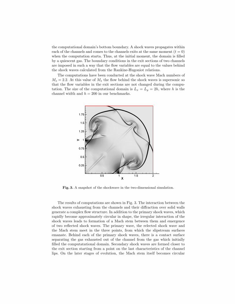
the computational domain’s bottom boundary. A shock waves propagates withineach of the channels and comes to the channels exits at the same moment (t = 0)when the computation starta. Thus, at the initial moment, the domain is filledby a quiescent gas. The boundary conditions in the exit sections of two channelsare imposed in such a way that the flow variables are equal to the values behindthe shock waves calculated from the Rankine-Hugoniot relations.

The computations have been conducted at the shock wave Mach numbers ofMs = 2.2. At this value of Ms the flow behind the shock waves is supersonic sothat the flow variables in the exit sections are not changed during the compu-tation. The size of the computational domain is Lx = Ly = 2h, where h is thechannel width and h = 200 in our benchmarks.

2.1 Simulation results

The computations have been conducted at the shock wave Mach numbers Ms =2.2. At this value of Ms the flow behind the shock waves is supersonic so thatthe flow variables in the exit sections are not changed during the computation.The sizes of computational domain are Lx = Ly = 2h, where h is the channelwidth. The computational grid consists of 400!400 cells.

The results of computations are shown in Figure 2.1. The interaction be-tween the shock waves exhausting from the channels and their di!raction oversolid walls generate a complex flow structure. In addition to the primary shockwaves, which rapidly become of an approximately circular shape, the irregularinteraction of the shock waves leads to formation of a Mach stem between themand emergence of two reflected shock waves. The primary wave, the relectedshock wave and the Mach stem meet in the triple points, from which slipstreamsurfaces are emanated. Behind each primary shock waves, there is a contact sur-face separating the gas exhausted from the channel from the gas which initiallyfilled the computatational domain. Secondary shock waves are formed closer tothe exit section starting from a point on the last characteristics of the channellip. On the later stages of evolution, the Mach stem itself becomes of circularshape and occupies the most portion of the leading shock front while the contactsurface behind it curls up into a mushroom-like structure.

Fig. 2. Results of the simulation using the SaC compiler

3 Performance, programmability and lessons learned

This section will be finalised in the complete version of the paper. At this stagewe can identify the following bullet points:

Fig. 3. A snapshot of the shockwave in the two-dimensional simulation.

The results of computations are shown in Fig. 3. The interaction between theshock waves exhausting from the channels and their diffraction over solid wallsgenerate a complex flow structure. In addition to the primary shock waves, whichrapidly become approximately circular in shape, the irregular interaction of theshock waves leads to formation of a Mach stem between them and emergenceof two reflected shock waves. The primary wave, the relected shock wave andthe Mach stem meet in the three points, from which the slipstream surfacesemanate. Behind each of the primary shock waves, there is a contact surfaceseparating the gas exhausted out of the channel from the gas which initiallyfilled the computatational domain. Secondary shock waves are formed closer tothe exit section starting from a point on the last characteristics of the channellips. On the later stages of evolution, the Mach stem itself becomes circular

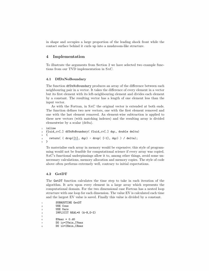
in shape and occupies a large proportion of the leading shock front while thecontact surface behind it curls up into a mushroom-like structure.

4 Implementation

To illustrate the arguments from Section 2 we have selected two example func-tions from our TVD implementation in SaC.

4.1 DfDxNoBoundary

The function dfDxNoBoundary produces an array of the difference between eachneighbouring pair in a vector. It takes the difference of every element in a vectorbut its first element with its left-neighbouring element and divides each elementby a constant. The resulting vector has a length of one element less than theinput vector.

As with the Fortran, in SaC the original vector is extended at both ends.The function defines two new vectors, one with the first element removed andone with the last element removed. An element-wise subtraction is applied tothese new vectors (with matching indexes) and the resulting array is dividedelementwise by a scalar (delta).

1 inline2 fluid_cv[.] dfDxNoBoundary( fluid_cv[.] dqc, double delta)3 {4 return( ( drop([1], dqc) - drop( [-1], dqc) ) / delta);5 }

To materialise each array in memory would be expensive; this style of program-ming would not be feasible for computational science if every array was copied.SaC’s functional underpinnings allow it to, among other things, avoid some un-necessary calculations, memory allocation and memory copies. The style of codeabove often performs extremely well, contrary to initial expectations.

4.2 GetDT

The GetDT function calculates the time step to take in each iteration of thealgorithm. It acts upon every element in a large array which represents thecomputational domain. For the two dimensional case Fortran has a nested loopstructure with one loop for each dimension. The value EV is calculated each timeand the largest EV value is saved. Finally this value is divided by a constant.

1 SUBROUTINE GetDT2 USE Cons3 USE Vars4 IMPLICIT REAL*8 (A-H,O-Z)5

6 EVmax = 0.d07 DO iy=IYmin,IYmax8 DO ix=IXmin,IXmax

9 Ux = QP(1,ix,iy)10 Uy = QP(2,ix,iy)11 Pc = QP(3,ix,iy)12 Rc = QP(4,ix,iy)13 C = SQRT(Gam*Pc/Rc)14 EV = (ABS(Ux)+C)/Dx+(ABS(Uy)+C)/Dy15 EVmax = MAX(EV,EVmax)16 END DO17 END DO18

19 DT = CFL/EVmax20

21 END

The SaC version of the function is shown below. In the following code GAM,DELTA and CFL are constants.

1 inline2 double getDt(fluid_pv[+] qp)3 {4 c = sqrt(GAM * p(qp) / rho(qp));5 d = MathArray::fabs( u(qp));6 ev = { iv -> (sum( ( d[iv] + c[iv]) / DELTA))};7 return( CFL / maxval( ev));8 }

The type of the function parameter is fluid_pv[+] which means an array ofunknown dimensionality of fluid_pv values, where fluid_pv is a user defineddatatype. The syntax for an array type (t) can be syntactically represented ast[x,y,z] for an array of size x by y by z, t[.,.] for a array of two dimensionsof unknown size and also t[+] for an array of unknown dimensionality.

The functions p and ρ extract the pressure and density from fluid_pv re-spectively. The SaC function calculates the variable C above using elementwiseoperations and then in line 6 EV is calculated, which depends on the entire inputarray. With little experience with SaC this function quickly becomes easier tounderstand than the Fortran code. It is a functional definition (i.e. an expres-sion) but the programmer is not obliged to use recursion on the array like afunctional programmer would do with lists.

This clearer imperative-like but functional style makes data dependenciesmore obvious both to the programmer and to the compiler. In our simulationthe SaC compiler always calculates the dimensionality needed for this functionfrom its calls and therefore no penalty is paid for the generic type of qp.

5 Results

To evaluate the performance of SaC compared with Fortran we ran the 2Dsimulation with a 400x400 grid as described in Section 3.2. The simulation wasrun for 1000 time steps to ensure that the run time was sufficient to negatethe start-up time of the program. We made use of a 400x400 grid as this wasthe size used in the original Fortran implementation. In the experiment we used

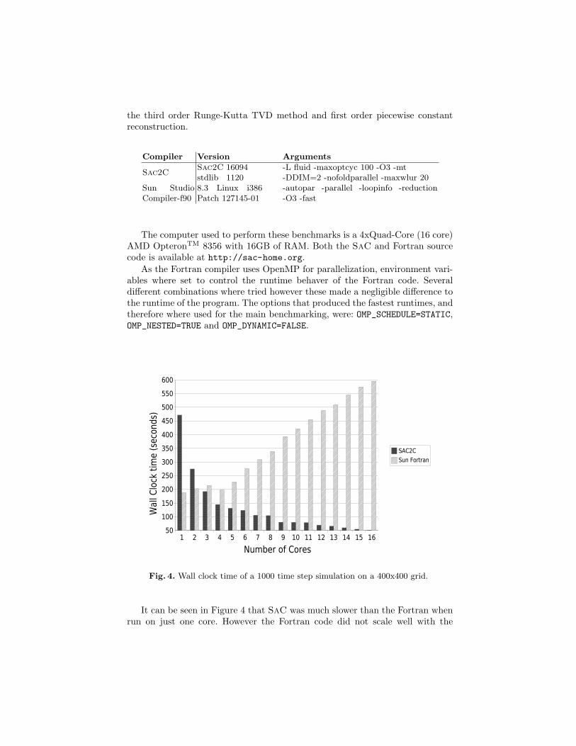
the third order Runge-Kutta TVD method and first order piecewise constantreconstruction.

Compiler Version Arguments

Sac2CSac2C 16094 -L fluid -maxoptcyc 100 -O3 -mt

-DDIM=2 -nofoldparallel -maxwlur 20stdlib 1120Sun StudioCompiler-f90

8.3 Linux i386Patch 127145-01

-autopar -parallel -loopinfo -reduction-O3 -fast

The computer used to perform these benchmarks is a 4xQuad-Core (16 core)AMD OpteronTM 8356 with 16GB of RAM. Both the SaC and Fortran sourcecode is available at http://sac-home.org.

As the Fortran compiler uses OpenMP for parallelization, environment vari-ables where set to control the runtime behaver of the Fortran code. Severaldifferent combinations where tried however these made a negligible difference tothe runtime of the program. The options that produced the fastest runtimes, andtherefore where used for the main benchmarking, were: OMP_SCHEDULE=STATIC,OMP_NESTED=TRUE and OMP_DYNAMIC=FALSE.

1 2 3 4 5 6 7 8 9 10 11 12 13 14 15 1650

100

150

200

250

300

350

400

450

500

550

600

SAC2C

Sun Fortran

Number of Cores

Wal

l Clo

ck t

ime

(sec

onds

)

Fig. 4. Wall clock time of a 1000 time step simulation on a 400x400 grid.

It can be seen in Figure 4 that SaC was much slower than the Fortran whenrun on just one core. However the Fortran code did not scale well with the

number of cores, and as the number of cores increased performance degraded.We therefore suspect that there is added overhead of communication betweenthe threads.

SaC does not use system calls for its inter-thread communication but ratheruses shared memory and spin locks to allow inter thread communication withvery little overhead. This low overhead allows SaC to scale well even when itsproblem size is too small for Fortran’s auto-parallelization feature to work effi-ciently. There are optimizations which the SaC compiler can perform which areonly possible because SaC is a functional, single assignment language. Theseoptimizations help to allow the program to scale by collating many small oper-ations on arrays into fewer, larger operations. This is not possible in proceduralprograming languages like Fortran as the compiler can not always work out thedata dependences in complete detail: with a functional language like SaC it ispossible to identify data dependencies.

When the same benchmark was run with a larger 2000x2000 grid we discov-ered that Fortran was able to scale slightly with small numbers of cores but afterjust five cores it started to suffer from the overheads of inter-thread communi-cation again.

6 Related Work

Broadly three techniques exist for producing highly parallelizable code for scien-tific simulations. The first technique is to carefully determine how a run shouldbe parallelised and to explicitly write the code to do this. The message pass-ing interface API[6] is commonly used for this. Also a threading library likePthreads [7] could be used. Secondly, source-code annotations or directives canbe used to provide information to a compiler to show it how an execution canbe parallelised. Lastly compilers can try to autoparallelize code by analysingdependencies between variables. This section gives a brief overview of the threemethods mentioned above and then discusses performance.

High-Performance Fortran [8] is an extension to FORTRAN-90 that allowsthe addition of directives to the source code to annotate distribution and locality.The Fortran code itself is written in a sequential style and already describes someoperations in a data-parallel way. High-Performance Fortran compilers can thenuse these directives to compile to pipelined, vectorized, SIMD or message passingparallel code.

For explicitly annotating parts of a program that can be parallelized onshared memory systems the OpenMP [9] API is supported for C, C++ andFortran. Many autoparallelizing compilers produce programs that call upon thisAPI including the Intel and Sun Microsystems Fortran and C compilers.

ZPL [10] is a high level array processing language designed to be conciseand platform independent. It allows programmers to easily describe subarrayswithin an array using a concept called regions. ZPL was designed with paral-lelism in mind and has had its performance compared with other languages forapplications inclusive of computational fluid dynamics applications [11].

Parallel performance results tend to vary depending on the application, ar-chitecture and type of parallelism. For example an application that performs wellon shared memory systems may not necessarily perform well when compiled torun on a distributed memory system. In addition and rather surprisingly, care-fully crafted MPI applications might not necessarily have better speedups percore than implicit parallelism in high level languages. One surprising exampleof this is ZPL which has been shown to scale well in parallel runs with theMultigrid [12] NAS benchmark [13] and even shown prospects with CFD [11].

7 Conclusion

The results have shown that execution of high-performance applications writtenin SaC can achieve speedups on parallel architectures. SaC provides a powerfulexpressiveness where the greater learning curve is not grasping the paradigm butin resisting the temptation to try to optimize the code, and thus making use ofSaC’s ability to allow programs to be written with a high level of abstraction.

Programmers need a good way to express their programs so that they arequick to write, easy to understand and efficient to maintain. Up until now ex-pressing programs in a readable form, with high levels of abstraction has comeat a considerable performance penalty. However, as can be seen in this paper itis possible to write programs in a clear style with high levels of abstraction whileobtaining reasonable speedups that can be greater than those produced from thecompilers of languages that where originally designed as sequential languages.

The results of this paper used SaC’s Pthread back-end; future SaC back-ends promise even more parallelism. CUDA [14], whilst challenging to harness,has tremendous processing capabilities that will enable programs to make use ofhigh performance, low cost processing resources found on GPUs as a potentiallyfaster way of performing complicated simulations [15]. As part of an EU FP-7 project a back-end is being developed for SaC which produces code for alanguage which will compile to a many-core architecture called Microgrid [16].This architecture will deliver considerable parallelism without the complexitythat is involved with CUDA.

For future architectures parallelism will be increasingly vital. The work inthis paper has shown that now that parallelism is important, it is possible towrite abstract code in a high-level language and still be able to compete withtraditional low-level, high performance languages like Fortran on parallel archi-tectures.

Acknowledgments This work was partly supported by the European FP-7 Integrated Project Apple-core (FP7-215216 — Architecture Paradigms andProgramming Languages for Efficient programming of multiple COREs).

References

1. Scholz, S.B.: Single assignment c — efficient support for high-level array operationsin a functional setting. Journal of Functional Programming 13 (2003) 1005–1059

2. et al, A.S.: Implementing a numerical solution of the kpi equation using singleassignment c: Lessons learned and experiences. In: Implementation and Applicationof Functional Languages, 20th international symposium. (2005) 160–170

3. Guinot, V.: Godunov-type schemes. Elsevier, Amsterdam (2003)4. Godunov, S.: A difference method for numerical calculation of discontinuous equa-

tions of hydrodynamics (in russian). Mat. Sb. 47 (1959) 271–3005. Sod, G.A.: A survey of several finite difference methods for systems of nonlinear

hyperbolic conservation laws. Journal of Computational Physics 27 (1978) 1–316. Forum, M.P.I.: MPI: A Message-Passing Interface Standard, Version 2.1. High

Performance Computing Center Stuttgart (HLRS) (2008)7. Josey, A.: The Single UNIX Specification Version 3. Open Group (2004)8. Forum, H.P.F.: High Performance Fortran Language Specification. Rice University

(1993)9. Chapman, B., Jost, G., Van Der Pas, R., Kuck, D.: Using OpenMP: portable

shared memory parallel programming. The MIT Press (2007)10. Lin, C., Snyder, L.: ZPL: An array sublanguage. Lecture Notes in Computer

Science 768 (1994) 96–11411. Lin, C., Snyder, L.: SIMPLE performance results in ZPL. Lecture Notes in Com-

puter Science 892 (1995) 361–37512. Briggs, W., McCormick, S.: A multigrid tutorial. Society for Industrial Mathe-

matics (2000)13. Chamberlain, B., Deitz, S., Snyder, L.: A comparative study of the NAS MG bench-

mark across parallel languages and architectures. In: Supercomputing, ACM/IEEE2000 Conference. (2000) 46–46

14. Guo, J., Thiyagalingam, J., Scholz, S.B.: Towards Compiling SAC to CUDA.In: Proceedings of the 10th Symposium On Trends In Functional Programming,Komarno, Slovakia (2009)

15. Senocak, I., Thibault, J., Caylor, M.: (J19. 2 Rapid-response Urban CFD Simula-tions using a GPU Computing Paradigm on Desktop Supercomputers)

16. Grelck, C., Herhut, S., Jesshope, C., Joslin, C., Lankamp, M., Scholz, S.B., Sha-farenko, A.: Compiling the Functional Data-Parallel Language sac for Microgridsof Self-Adaptive Virtual Processors. In: 14th Workshop on Compilers for ParallelComputing (CPC09), IBM Research Center, Zurich, Switzerland. (2009)