Embed Size (px)
Citation preview

Applied Mathematical Modelling 36 (2012) 605–617
Contents lists available at ScienceDirect
Applied Mathematical Modelling
journal homepage: www.elsevier .com/locate /apm
Numerical solutions of the generalized Kuramoto–Sivashinskyequation using B-spline functions
Mehrdad Lakestani a, Mehdi Dehghan b,⇑a Faculty of Mathematical Sciences, University of Tabriz, Tabriz, Iranb Department of Applied Mathematics, Faculty of Mathematics and Computer Sciences, Amirkabir University of Technology, No. 424, Hafez Avenue,15914 Tehran, Iran
a r t i c l e i n f o
Article history:Received 16 August 2010Received in revised form 29 May 2011Accepted 1 July 2011Available online 3 August 2011
Keywords:B-spline functionKuramoto–Sivashinsky equationDerivative matrixCollocation method
0307-904X/$ - see front matter � 2011 Elsevier Incdoi:10.1016/j.apm.2011.07.028
⇑ Corresponding author. Tel.: +98 21 64542503; fE-mail addresses: [email protected], lakesta
a b s t r a c t
A numerical technique based on the finite difference and collocation methods is presentedfor the solution of generalized Kuramoto–Sivashinsky (GKS) equation. The derivativematrices between any two families of B-spline functions are presented and are utilizedto reduce the solution of GKS equation to the solution of linear algebraic equations. Numer-ical simulations for five test examples have been demonstrated to validate the techniqueproposed in the current paper. It is found that the simulating results are in good agreementwith the exact solutions.
� 2011 Elsevier Inc. All rights reserved.
1. Introduction
As is said in [1] the generalized Kuramoto–Sivashinsky (GKS) equation is a model of nonlinear partial differential equation(NLPDE) frequently encountered in the study of continuous media which exhibits a chaotic behavior form
@u@tþ u
@u@xþ a
@2u@x2 þ b
@3u@x3 þ c
@4u@x4 ¼ 0; ð1:1Þ
where a, b and c are nonzero real constants.For b = 0, Eq. (1.1) is called the Kuramoto–Sivashinsky (KS) equation which is a canonical nonlinear evolution equation
arising in a variety of physical contexts, e.g. long waves on thin films, unstable drift waves in plasmas, reaction diffusion sys-tems [2], etc. This equation was originally derived in the context of plasma instabilities, flame front propagation, and phaseturbulence in reaction–diffusion system [3]. It appears in context of long waves on the interface between two viscous fluids[4], unstable drift waves in plasmas, and flame front instability [5]. The Kuramoto–Sivashinsky equation models the fluctu-ations of the position of a flame front, the motion of a fluid going down a vertical wall, or a spatially uniform oscillatingchemical reaction in a homogeneous medium [6]. This equation is useful to model solitary pulses in a falling thin film[7]. As is mentioned in [8] this equation can be precisely recovered from a model in the continuity equation by adding anappropriate amending-function.
For a = c = 1 and b = 0 it represents models of pattern formation on unstable flame fronts and thin hydrodynamic films [5],Eq. (1.1) has thus been studied extensively [9,10].
. All rights reserved.
ax: +98 21 [email protected] (M. Lakestani), [email protected], [email protected] (M. Dehghan).

606 M. Lakestani, M. Dehghan / Applied Mathematical Modelling 36 (2012) 605–617
In the past several years ago, various methods have been proposed to solve this equation. Authors of [1] presented theChebyshev spectral collocation scheme to solve this equation. This equation is solved by lattice Boltzmann technique [8].The method of radial basis functions [11,12] developed in [13] to find the approximate solution of this equation. Authorsof [14] proposed the local discontinuous Galerkin methods to solve this equation. The tanh function method is developedin [15] and author of [16] investigated this equation and proposed a technique based on the variational iteration method[17]. More investigations can be found in [18,19].
It is worth to point out that, recently various methods have been proposed to construct exact solutions of Kuramoto–Sivashinsky equation. For more details we refer the interested reader to [20–23]. Also many methods were developed forfinding exact solutions of some nonlinear evolution equations [24–28].
We would like to mention that this equation is also called KdV–Burgers–Kuramoto (KBK) equation. Thus the interestedreader can see [16,29,30].
The approach in the current paper is different. A numerical technique based on the finite difference [31,32] and colloca-tion methods [33,34] is proposed for the solution of generalized Kuramoto–Sivashinsky (GKS) equation. In this work we re-duce the given problem to a set of algebraic equations by expanding the unknown function as fifth order B-spline functionsspecially constructed on bounded intervals, with unknown coefficients. The derivative matrices between any two families ofB-spline functions are given. These matrices together with the B-spline functions are then utilized to evaluate the unknowncoefficients.
This paper is organized as follows: In Section 2, we describe the formulation of the B-spline functions on [a,b], and thederivative matrices required for our subsequent development. In Section 3 the proposed method is used to approximatethe solution of the problem in interval [a,b]. As the results a set of algebraic equations is formed and a solution of the con-sidered problem is introduced. In Section 4 the theoretical stability of the linearized scheme is presented. In Section 5, wereport our computational results and demonstrate the accuracy of the proposed approximate scheme by presenting numer-ical examples. Section 6 completes this paper with a brief conclusion. Note that we have computed the numerical results byMaple programming.
2. B-spline functions on [a,b]
The mth-order cardinal B-spline Nm(t) has the knot sequence {. . .,�1,0,1, . . .} and consists of polynomials of order m (de-gree m � 1) between the knots. Let N1(t) = v[0,1](t) be the characteristic function of [0,1]. Then for each integer m P 2, themth-order cardinal B-spline is defined, inductively by [35,36]
NmðtÞ ¼ ðNm�1 � N1ÞðtÞ ¼Z 1
�1Nm�1ðt � xÞN1ðxÞdx ¼
Z 1
0Nm�1ðt � xÞdx: ð2:1Þ
It can be shown [37] that Nm(t) for m P 2 can be achieved by using the following formula
NmðtÞ ¼t
m� 1Nm�1ðtÞ þ
m� tm� 1
Nm�1ðt � 1Þ;
recursively, and supp[Nm(t)] = [0,m].It can be seen [36] that a finite-energy sequence g[m,k] exists such that the relation
NmðtÞ ¼X
k
g½m; k�Nmð2t � kÞ; ð2:2Þ
where
g½m; k� ¼2�mþ1
m
k
!; 0 6 k 6 m;
0; elsewhere;
8>><>>:
is satisfied. The explicit expressions of N2(t), N3(t), N4(t) and N5(t) are [35–37]:
N2ðtÞ ¼
t; t 2 ½0;1�;
2� t; t 2 ½1;2�;
0; elsewhere;
8>><>>: ð2:3Þ
N3ðtÞ ¼12
t2; t 2 ½0;1�;
�2t2 þ 6t � 3; t 2 ½1;2�;
t2 � 6t þ 9; t 2 ½2;3�;
0; elsewhere;
8>>>>><>>>>>:
ð2:4Þ

M. Lakestani, M. Dehghan / Applied Mathematical Modelling 36 (2012) 605–617 607
N4ðtÞ ¼16
t3; t 2 ½0;1�;4� 12t þ 12t2 � 3t3; t 2 ½1;2�;�44þ 60t � 24t2 þ 3t3; t 2 ½2;3�;64� 48t þ 12t2 � t3; t 2 ½3;4�;0; elsewhere;
8>>>>>><>>>>>>:
ð2:5Þ
N5ðtÞ ¼1
24
t4; t 2 ½0;1�;�5þ 20t � 30t2 þ 20t3 � 4t4; t 2 ½1;2�;155� 300t þ 210t2 � 60t3 þ 6t4; t 2 ½2;3�;�655þ 780t � 330t2 þ 60t3 � 4t4; t 2 ½3;4�;625� 500t þ 150t2 � 20t3 þ t4; t 2 ½4;5�;0; elsewhere:
8>>>>>>>><>>>>>>>>:
ð2:6Þ
Suppose Ni;j;kðtÞ ¼ Nið2jt � kÞ; i ¼ 1;2;3;4;5; j; k 2 R and Bi,j,k = supp[Ni,j,k(t)] = clos{t:Ni,j,k(t) – 0}. It is easy to see that
Bi;j;k ¼ ½2�jk;2�jðiþ kÞ�; i ¼ 1; . . . ;5 j; k 2 R:
Define the set of indices
Si;j ¼ fk : Bi;j;k \ ða; bÞ – ;g; i ¼ 1; . . . ;5; j 2 R;
and suppose mi;j ¼ minfSi;jg and Mi;j ¼ maxfSi;jg; i ¼ 1; . . . ;5; j 2 R.We need that these functions intrinsically defined on [a,b] so we put
Nij;kðtÞ ¼ Ni;j;kðtÞv½a;b�ðtÞ; i ¼ 1; . . . ;5; j 2 R; k 2 Si;j: ð2:7Þ
2.1. The function approximation
Suppose
Ui;jðtÞ ¼ Nij;mi;jðtÞ;Ni
j;mi;jþ1ðtÞ; . . . ;Nij;Mi;jðtÞ
h iT; i ¼ 1; . . . ;5; j 2 R: ð2:8Þ
For a fixed j = J, a function f(t) defined over [a,b] may be represented by the fifth order B-spline functions as
f ðtÞ ¼XM5;J
k¼m5;J
skN5J;kðtÞ ¼ STU5;JðtÞ; ð2:9Þ
where
S ¼ ½sm5;J ; sm5;Jþ1; . . . ; sM5;J �T; ð2:10Þ
where sk; k ¼ m5;J; . . . ;M5;J , can be found using the method presented in [38].
2.2. The derivative matrices
Using Eq. (2.1) we get [36]
NmðtÞ0 ¼ddt
NmðtÞ ¼ Nm�1ðtÞ � Nm�1ðt � 1Þ: ð2:11Þ
Now using Eqs. (2.8) and (2.11) we obtain
U0i;JðtÞ ¼ Di;JUi�1;JðtÞ; i ¼ 2;3;4;5; ð2:12Þ
where
Di;J ¼ 2J �
�11 �1
. .. . .
.
1 �11
26666664
37777775; i ¼ 2;3;4;5;
and Di,J is a ðMi;J �mi;JÞ � ðMi;J �mi;J � 1Þ matrix. Because supp[Nm(t)] = [0,m], it can be found thatMi;J �mi;J � 1 ¼Mi�1;J �mi�1;J .

608 M. Lakestani, M. Dehghan / Applied Mathematical Modelling 36 (2012) 605–617
3. Description of the numerical method
Consider the GKS equation (1.1) with initial value
uðx;0Þ ¼ hðxÞ; x 2 ½a; b�; ð3:1Þ
and boundary conditions
uða; tÞ ¼ f1ðtÞ;uðb; tÞ ¼ f2ðtÞ;uxða; tÞ ¼ g1ðtÞ;uxðb; tÞ ¼ g2ðtÞ;
8>>><>>>:
ð3:2Þ
where h(x), f1(t), f2(t), g1(t) and g2(t) are known functions.Here we introduce a numerical scheme to solve the problem.
3.1. Scheme based on Crank–Nicolson time stepping
By integrating form Eq. (1.1) with respect to ‘‘t’’ in the interval [t, t + dt] we get
uðx; t þ dtÞ � uðx; tÞ þZ tþdt
tuðx; tÞuxðx; tÞdt þ a
Z tþdt
tuxxðx; tÞdt þ b
Z tþdt
tuxxxðx; tÞdt þ c
Z tþdt
tuxxxxðx; tÞdt ¼ 0: ð3:3Þ
Using the trapezoid method we can approximate Eq. (3.3) as
uðx; t þ dtÞ � uðx; tÞ þ dt2fuðx; t þ dtÞuxðx; t þ dtÞ þ uðx; tÞuxðx; tÞg þ a
dt2fuxxðx; t þ dtÞ þ uxxðx; tÞg þ b
dt2fuxxxðx; t þ dtÞ
þ uxxxðx; tÞg þ cdt2fuxxxxðx; t þ dtÞ þ uxxxxðx; tÞg ¼ 0; ð3:4Þ
where dt is the time step size. To linearize the non-linear term u(x, t + dt)ux(x, t + dt) we use the linearization form given byRubin and Graves [39]
uðx; t þ dtÞuxðx; t þ dtÞ � uðx; t þ dtÞuxðx; tÞ þ uðx; tÞuxðx; t þ dtÞ � uðx; tÞuxðx; tÞ: ð3:5Þ
Replacing Eq. (3.5) in Eq. (3.4), then rearranging it, and using the notation un = u(x, tn) where tn = tn�1 + dt, we obtain
unþ1 � un þ dt2
unþ1run þ unrunþ1 þ a r2unþ1 þr2un� �
þ b r3unþ1 þr3un� �
þ c r4unþ1 þr4un� �n o
¼ 0; ð3:6Þ
where r is the gradient operator.Using Eq. (2.9), the function u(x, tn) can be approximated as
unðxÞ ¼XM5;J
k¼m5;J
unkN5
J;kðxÞ ¼ UTnU5;JðxÞ; ð3:7Þ
where Un ¼ unm5;J; un
m5;Jþ1; . . . ; unM5;J
h iT, and U5,J(x) is defined as (2.8).
Also using (2.12) we can write
run ¼ UTn
ddx
U5;JðxÞ ¼ UTnD5;JU4;JðxÞ; ð3:8Þ
r2un ¼ UTn
d2
dx2 U5;JðxÞ ¼ UTnD5;J
ddx
U4;JðxÞ ¼ UTnD5;JD4;JU3;JðxÞ; ð3:9Þ
r3un ¼ UTn
d3
dx3 U5;JðxÞ ¼ UTnD5;JD4;JD3;JU2;JðxÞ; ð3:10Þ
r4un ¼ UTn
d4
dx4 U5;JðxÞ ¼ UTnD5;JD4;JD3;JD2;JU1;JðxÞ: ð3:11Þ
Replacing Eqs. (3.7)–(3.11) in Eq. (3.6) we get
UT5;JðxÞ 1þ dt
2UT
4;JðxÞDT5;JUn þUnU
T4;JðxÞD
T5;J
� �� �þ dt
2aUT
3;JðxÞDT4;JD
T5;J þ bUT
2;JðxÞDT3;JD
T4;JD
T5;J þ cUT
1;JðxÞDT2;JD
T3;JD
T4;JD
T5;J
� �� �Unþ1
¼ UT5;JðxÞ �
dt2
aUT3;JðxÞD
T4;JD
T5;J þ bUT
2;JðxÞDT3;JD
T4;JD
T5;J þ cUT
1;JðxÞDT2;JD
T3;JD
T4;JD
T5;J
� �� �Un:
ð3:12Þ

M. Lakestani, M. Dehghan / Applied Mathematical Modelling 36 (2012) 605–617 609
Using Eqs. (3.7) and (3.8) in (3.2) we have
UT5;JðaÞUnþ1 ¼ f1ðtnþ1Þ;
UT5;JðbÞUnþ1 ¼ f2ðtnþ1Þ;
UT4;JðaÞD
T5;JUnþ1 ¼ g1ðtnþ1Þ;
UT4;JðbÞD
T5;JUnþ1 ¼ g2ðtnþ1Þ:
ð3:13Þ
Collocating Eq. (3.12) in ‘ ¼Mi;J �mi;J � 4 points xi = i(b � a)/(‘ + 1) + a, i = 1,2, . . . ,‘ we get
UT5;JðxiÞ 1þ dt
2UT
4;JðxiÞDT5;JUn þ UnU
T4;JðxiÞDT
5;J
� �� �þ dt
2aUT
3;JðxiÞDT4;JD
T5;J þ bUT
2;JðxiÞDT3;JD
T4;JD
T5;J þ cUT
1;JðxiÞDT2;JD
T3;JD
T4;JD
T5;J
� �� �Unþ1
¼ UT5;JðxiÞ �
dt2
aUT3;JðxiÞDT
4;JDT5;J þ bUT
2;JðxiÞDT3;JD
T4;JD
T5;J þ cUT
1;JðxiÞDT2;JD
T3;JD
T4;JD
T5;J
� �� �Un:
ð3:14Þ
Writing (3.14) together with (3.13) in a matrix form we have
AnUnþ1 ¼ bn; n ¼ 1;2; . . . ; ð3:15Þ
where An is a (‘ + 3) � (‘ + 3) matrix as
An :¼
UT5;JðaÞ
UT4;JðaÞD
T5;J
n1
..
.
n‘UT
5;JðbÞUT
4;JðbÞDT5;J
266666666666664
377777777777775;
and
bn :¼
f1ðtnþ1Þg1ðtnþ1Þ
f1
..
.
f‘f2ðtnþ1Þg2ðtnþ1Þ
26666666666664
37777777777775;
with
ni ¼ UT5;JðxiÞ 1þ dt
2UT
4;JðxiÞDT5;JUn þ UnU
T4;JðxiÞDT
5;J
� �� �
þ dt2
aUT3;JðxiÞDT
4;JDT5;J þ bUT
2;JðxiÞDT3;JD
T4;JD
T5;J þ cUT
1;JðxiÞDT2;JD
T3;JD
T4;JD
T5;J
� �; i ¼ 1;2; . . . ; ‘;
and
fi ¼ UT5;JðxiÞ �
dt2
aUT3;JðxiÞDT
4;JDT5;J þ bUT
2;JðxiÞDT3;JD
T4;JD
T5;J þ cUT
1;JðxiÞDT2;JD
T3;JD
T4;JD
T5;J
� �� �Un; i ¼ 1;2; . . . ; ‘:
Eq. (3.15) using Eq. (3.1) as the starting points, gives a linear system of equations with ‘ + 4 unknowns and equations, whichcan be solved to find Un+1 in any step n = 1, . . .. So the unknown functions u(x, tn) in any time t = tn, n = 1,2, . . . can be found.
4. Theoretical stability of the linearized scheme
We use the notation of asymptotic stability of a numerical method as it is defined in [40] for a discrete problem of theform
dUdt¼ LJU;
where LJ is assumed to be a diagonalizable matrix.

610 M. Lakestani, M. Dehghan / Applied Mathematical Modelling 36 (2012) 605–617
Definition 1. The region of absolute stability of a numerical method is defined for the scalar model problem
dUdt¼ kU;
to be the set of all kdt such that kUnk is bounded as t ?1. We say that a numerical method is asymptotically stable for aparticular problem if for sufficiently small dt > 0, the product of the dt times every eigenvalue of L lies within the regionof absolute stability [41].
The Crank–Nicolson scheme: This method is absolutely stable in the entire left-half plane.
4.1. Stability for linearized GKS equation
We consider the linearized GKS equation
@u@tþ l @u
@xþ a
@2u@x2 þ b
@3u@x3 þ c
@4u@x4 ¼ 0; ð4:1Þ
where the linearization coefficient l stands for values of u. We assume that jlj 6M, where M is an upper bound of u. HereL = C�1K, where C and K are matrices in the form C = (V1,V2, . . . ,V‘+4) and K = (C1,C2, . . . ,C‘+4) where Vi and Ci, i = 1,2, . . . ,‘ + 4are the vectors in the forms
Vi ¼ �U5;JðxiÞ; i ¼ 1;2; . . . ; ‘þ 4;
and
Ci ¼ � lD5;JU4;JðxiÞ þ aD5;JD4;JU3;JðxiÞ þ bD5;JD4;JD3;JU2;JðxiÞ þ cD5;JD4;JD3;JD2;JU1;JðxiÞ�
; i ¼ 1;2; . . . ; ‘þ 4;
respectively, so that the discretized linearized GKS equation becomes
dUdt¼ LU:
The Crank–Nicolson scheme is A-stable. The region of absolute stability for the Crank–Nicolson time stepping scheme isplotted in Fig. 1, for Examples 1 and 2 presented in this paper.
5. Numerical examples
In this section we give some computational results of numerical experiments with the method based on Section 3, to sup-port our theoretical discussion.
Fig. 1. dt = 10�3 times the eigenvalues of L1 for Example 1 (left) and Example 2 (right).

Table 1Ł1 and L2 errors for u(t) using presented method.
dt Ł1-error L2-error Ł1-error L2-errorJ = 4 J = 4 J = 5 J = 5
0.1 7.3 � 10�3 6.5 � 10�3 4.4 � 10�3 3.7 � 10�3
0.01 6.1 � 10�3 5.7 � 10�3 3.3 � 10�5 2.6 � 10�5
0.001 1.0 � 10�4 8.4 � 10�5 2.8 � 10�6 1.5 � 10�6
Fig. 3. Plot of exact and approximate solutions for J = 1, dt = 0.1, T = 1 (left) and T = 2 (right) for Example 1.
Fig. 2. Plot of exact and approximate solutions for J = 1, dt = 0.01, T = 0.5 (left) and T = 1 (right) for Example 1.
M. Lakestani, M. Dehghan / Applied Mathematical Modelling 36 (2012) 605–617 611

Fig. 4. Plot of exact and approximate solutions for J = 1, dt = 0.2, T = 1 (left) and T = 2 (right) for Example 1.
Fig. 5. Plot of exact and approximate solutions for J = 2, dt = 0.2, T = 1 (left) and T = 2 (right) for Example 1.
612 M. Lakestani, M. Dehghan / Applied Mathematical Modelling 36 (2012) 605–617
Example 1. In this example, we consider the GKS equation, represented by a = c = 1 and b = 4. The exact solution is [1]
uðx; tÞ ¼ 11þ 15 tanhh� 15 tanh2 h� 15 tanh3 h;
with h ¼ � 12 xþ t. We will use this solution, evaluated at t = 0, as the initial condition, and the boundary functions from the
exact solution on the interval [�1,1]. The Ł1 and L2 errors are obtained in Table 1 for the presented method in time t = 1 fordifferent values of dt and J.
Figs. 2–6 show the chaotic solutions for different values of J, T, dt on the interval [�10,10].
Example 2. Consider Eq. (1.1) with a = 2, c = 1 and b = 0. The exact solution is [1]
uðx; tÞ ¼ � 1jþ 60
19jð�38cj2 þ aÞ tanhhþ 120cj3 tanh3 h;

Fig. 6. Plot of exact and approximate solutions for J = 2, dt = 0.2, T = 3 (left) and T = 4 (right) for Example 1.
Table 2Ł1 and L2 errors for u(t) using the presented method.
dt Ł1-error L2-error Ł1-error L2-errorJ = 4 J = 4 J = 5 J = 5
0.1 1.3 � 10�3 1.2 � 10�3 1.7 � 10�3 1.5 � 10�3
0.01 4.2 � 10�4 3.7 � 10�4 9.0 � 10�5 8.0 � 10�5
0.001 9.7 � 10�5 9.1 � 10�5 6.2 � 10�6 5.5 � 10�6
Fig. 7. Plot of exact and approximate solutions for J = 1, dt = 0.01, T = 0.5 (left) and T = 1 (right) for Example 2.
M. Lakestani, M. Dehghan / Applied Mathematical Modelling 36 (2012) 605–617 613
where h = jx + t and j ¼ ð1=2Þffiffiffiffiffiffiffiffiffiffiffiffiffiffiffiffiffiffiffi11a=19c
p. Similar to the previous example, we extract the required boundary functions from
the exact solution on the interval [�1,1]. The Ł1 and L2 errors are obtained in Table 2 for the presented method in time t = 1for different values of dt and J. Figs. 7 and 8 show the chaotic solutions for different values of J, T, dt on the interval [�10,10].
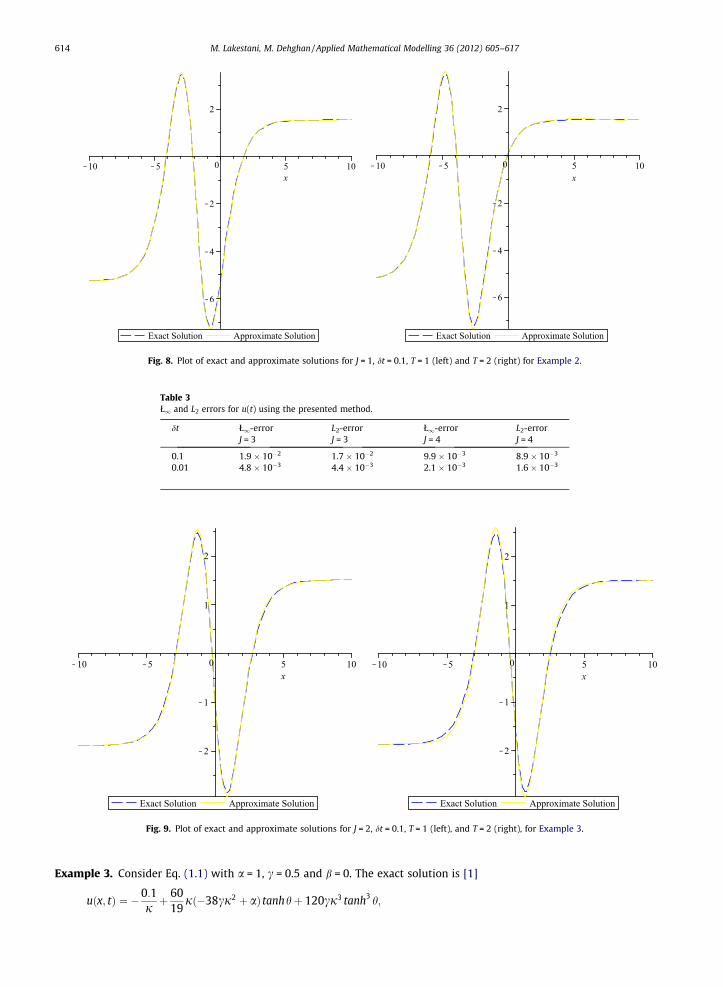
Fig. 8. Plot of exact and approximate solutions for J = 1, dt = 0.1, T = 1 (left) and T = 2 (right) for Example 2.
Table 3Ł1 and L2 errors for u(t) using the presented method.
dt Ł1-error L2-error Ł1-error L2-errorJ = 3 J = 3 J = 4 J = 4
0.1 1.9 � 10�2 1.7 � 10�2 9.9 � 10�3 8.9 � 10�3
0.01 4.8 � 10�3 4.4 � 10�3 2.1 � 10�3 1.6 � 10�3
Fig. 9. Plot of exact and approximate solutions for J = 2, dt = 0.1, T = 1 (left), and T = 2 (right), for Example 3.
614 M. Lakestani, M. Dehghan / Applied Mathematical Modelling 36 (2012) 605–617
Example 3. Consider Eq. (1.1) with a = 1, c = 0.5 and b = 0. The exact solution is [1]
uðx; tÞ ¼ �0:1jþ 60
19jð�38cj2 þ aÞ tanhhþ 120cj3 tanh3 h;

Fig. 10. The chaotic solution of the GKS equation for J = 1, dt = 0.1, t 2 [0,5], for Example 3.
Table 4Ł1 error for u(t) using CN method.
c CN method Method [1]
0.1 7.7 � 10�7 2.6 � 10�4
0.01 1.8 � 10�6 3.2 � 10�5
0.001 1.6 � 10�6 3.2 � 10�5
M. Lakestani, M. Dehghan / Applied Mathematical Modelling 36 (2012) 605–617 615
where h = jx + 0.1t and j ¼ ð1=2Þffiffiffiffiffiffiffiffiffiffiffiffiffiffiffiffiffiffiffi11a=19c
p. Again, we extract the required boundary functions from the exact solution on
the interval [�1,1]. The Ł1 and L2 errors are obtained in Table 3 for the presented method in time t = 1 for different values ofdt and J. Fig. 9 shows the chaotic solutions for J = 2, dt = 0.1 and T = 1, 2 on the interval [�10,10]. The chaotic solutions areshown in Fig. 10 for J = 1, dt = 0.1 and t 2 [0,5].
Example 4. Consider Eq. (1.1) with a = 1,c = 1 and b = 4. The exact solution is [1]
uðx; tÞ ¼ 9þ 2c þ 15 tanhh� 15 tanh2 h� 15 tanh3 h;
where h = �1/2x + ct. Similar to the previous examples, we extract the required boundary functions from the exact solutionon the interval [�1,1]. The Ł1 errors for different values of c are obtained in Table 4 for the presented method in time t = 1 fordt = 0.05 and J = 5, also we compare the results with the method proposed in [1].
Example 5. In this example, we consider another type of Kuramoto–Sivashinsky equation
ut þ uux þ uxx þ uxxxx ¼ 0;
where is the simplest nonlinear partial differential exhibiting the chaotic behavior over a finite spatial domain. Here we takethe Gaussian initial condition [13,42]
uðx;0Þ ¼ expð�x2Þ;
with the boundary conditions
uða; tÞ ¼ 0; uðb; tÞ ¼ 0; uxða; tÞ ¼ 0; uxðb; tÞ ¼ 0:
The numerical results are presented in Fig. 11 for a = �30 and b = 30. We can observe that the numerical results are conver-gent for the very chaotic nature.

Fig. 11. The chaotic solution of the KS equation for J = 1, dt = 0.1, t 2 [0,30], for Example 5.
616 M. Lakestani, M. Dehghan / Applied Mathematical Modelling 36 (2012) 605–617
6. Conclusion
In this paper we presented a numerical scheme for solving the generalized Kuramoto–Sivashinsky equation. The methodemployed to find the solution of this equation is based on the B-spline functions. The new method was applied on severaltest problems from the literature. The computational results are found to be in good agreement with the exact solutions. Thealgorithms proposed in the current paper can be employed to solve a large class of linear and nonlinear time-dependent par-tial differential equations.
Acknowledgments
The authors are very grateful to both referees for carefully reading the paper and for comments and suggestions whichhave improved the paper.
References
[1] A.H. Khater, R.S. Temsah, Numerical solutions of the generalized Kuramoto–Sivashinsky equation by Chebyshev spectral collocation methods, Comput.Math. Appl. 56 (2008) 1465–1472.
[2] Y. Kuramoto, T. Tsuzuki, Persistent propagation of concentration waves in dissipative media far from thermal equilibrium, Prog. Theor. Phys. 55 (1976)356–369.
[3] J. Rademacher J, R. Wattenberg, Viscous shocks in the destabilized Kuramoto–Sivashinsky, J. Comput. Nonlinear Dynam. 1 (2006) 336–347.[4] A.P. Hooper, R. Grimshaw, Nonlinear instability at the interface between two viscous fluids, Phys. Fluids 28 (1985) 37–45.[5] G.I. Sivashinsky, Instabilities, pattern-formation, and turbulence in flames, Ann. Rev. Fluid Mech. 15 (1983) 179–199.[6] R. Conte R, Exact solutions of nonlinear partial differential equations by singularity analysis, in: Lecture Notes in Physics, Springer, Berlin,
2003, pp. 1–83.[7] S. Demekhin Saprykin, EA. Kalliadasis, Two-dimensional wave dynamics in thin films, I. Stationary solitary pulses, J. Phys. Fluids 17 (2005) 1–16.[8] H. Lai, C.F. Ma, Lattice Boltzmann method for the generalized Kuramoto–Sivashinsky equation, Physica A 388 (2009) 1405–1412.[9] R. Grimshaw, A.P. Hooper, The non-existence of a certain class of travelling wave solutions of the Kuramoto–Sivashinsky equation, Physica D 50 (1991)
231–238.[10] X. Liu, Gevrey class regularity and approximate inertial manifolds for the Kuramoto–Sivashinsky equation, Physica D 50 (1991) 135–151.[11] M. Dehghan, A. Shokri, A numerical method for solution of the two-dimensional sine-Gordon equation using the radial basis functions, Math. Comput.
Simulat. 79 (2008) 700–715.[12] M. Tatari, M. Dehghan, On the solution of the non-local parabolic partial differential equations via radial basis functions, Appl. Math. Model. 33 (2009)
1729–1738.[13] M. Uddin, Sirajul Haq, Siraj-ul Islam, A mesh-free numerical method for solution of the family of Kuramoto–Sivashinsky equations, Appl. Math.
Comput. 212 (2009) 458–469.[14] Yan Xu, Chi-Wang Shu, Local discontinuous Galerkin methods for the Kuramoto–Sivashinsky equations and the Ito-type coupled KdV equations,
Comput. Methods Appl. Mech. Eng. 195 (2006) 3430–3447.[15] E. Fan, Extended tanh-function method and its applications to nonlinear equations, Phys. Lett. A 277 (2000) 212–218.[16] A.A. Soliman, A numerical simulation and explicit solutions of KdV–Burgers and Lax’s seventh-order KdV equations, Chaos Solitions Fract. 29 (2006)
294–302.[17] M. Tatari, M. Dehghan, On the convergence of He’s variational iteration method, J. Comput. Appl. Math. 207 (2007) 121–128.[18] H. Chen, H. Zhang, New multiple soliton solutions to the general Burgers–Fisher equation and the Kuramoto–Sivashinsky equation, Chaos Solitions
Fract. 19 (2004) 71–76.

M. Lakestani, M. Dehghan / Applied Mathematical Modelling 36 (2012) 605–617 617
[19] Tian-Shiang Yang, On traveling-wave solutions of the Kuramoto–Sivashinsky equation, Physica D 110 (1997) 25–42.[20] D. Baldwin, O. Goktas, W. Hereman, L. Hong, R.S. Martino, J.C. Miller, Symbolic computation of exact solutions expressible in hyperbolic and elliptic
functions for nonlinear PDEs, J. Symbolic Comput. 37 (2004) 669–705.[21] H. Triki, T.R. Taha, A.M. Wazwaz, Solitary wave solutions for a generalized KdV–mKdV equation with variable coefficients, Math. Comput. Simulat. 80
(2010) 1867–1873.[22] A.M. Wazwaz, An analytical study of compacton solutions for variants of Kuramoto–Sivashinsky equation, Appl. Math. Comput. 148 (2004) 571–585.[23] A.M. Wazwaz, Partial Differential Equations and Solitary Waves Theory, HEP and Springer, Peking and Berlin, 2009.[24] A.H. Khater, M.M. Hassan, R.S. Temsah, Exact solutions with Jacobi elliptic functions of two nonlinear models for ion-acoustic plasma waves, J. Phys.
Soc. Jpn. 74 (2005) 1431–1435.[25] A.H. Khater, A.A. Hassan, R.S. Temsah, Cnoidal wave solutions for a class of fifth-order KdV equations, Math. Comput. Simulat. 70 (2005) 221–226.[26] A.H. Khater, W. Malfliet, D.K. Callebaut, E.S. Kamel, Travelling wave solutions of some classes of nonlinear evolution equations in (1 + 1) and (2 + 1)
dimensions, J. Comput. Appl. Math. 140 (2002) 469–477.[27] A.H. Khater, W. Malfliet, D.K. Callebaut, E.S. Kamel, The tanh method, a simple transformation and exact analytical solutions for nonlinear reaction–
diffusion equations, Chaos Solitons Fract. 14 (2002) 513–522.[28] A.H. Khater, W. Malfliet, E.S. Kamel, Travelling wave solutions of some classes of nonlinear evolution equations in (1 + 1) and higher dimensions, Math.
Comput. Simulat. 64 (2004) 247–258.[29] M.A. Helal, M.S. Mehanna, A comparison between two different methods for solving KdV–Burgers equation, Chaos Solitions Fract. 28 (2006) 320–326.[30] C.F. Ma, A new lattice Boltzmann model for KdV–Burgers equation, Chinese Phys. Lett. 22 (2005) 2313–2315.[31] M. Dehghan, Finite difference procedures for solving a problem arising in modeling and design of certain optoelectronic devices, Math. Comput.
Simulat. 71 (2006) 16–30.[32] M. Dehghan, On the solution of an initial-boundary value problem that combines Neumann and integral condition for the wave equation, Numer.
Methods Part. Diff. Equat. 21 (2005) 24–40.[33] M. Dehghan, Implicit collocation technique for heat equation with non-classic initial condition, Int. J. Nonlinear Sci. Numer. Simulat. 7 (2006) 447–450.[34] M. Dehghan, F. Fakhar–Izadi, The spectral collocation method with three different bases for solving a nonlinear partial differential equation arising in
modeling of nonlinear waves, Math. Comput. Model. 53 (2011) 1865–1877.[35] C.K. Chui, An Introduction to Wavelets, Academic Press, San Diego, CA, 1992.[36] J.C. Goswami, A.K. Chan, Fundamentals of Wavelets: Theory, Algorithms, and Applications, John Wiley & sons, Inc., 1999.[37] C. de Boor, A Practical Guide to Spline, Springer-Verlag, New York, 1978.[38] M. Lakestani, M. Dehghan, Numerical solution of Riccati equation using the cubic B-spline scaling functions and Chebyshev cardinal functions, Comput.
Phys. Commun. 181 (2010) 957–966.[39] S.G. Rubin, R.A. Graves, Cubic spline approximation for problems in fluid mechanics, NASA TR R-436, Washington, DC, 1975.[40] C. Canuto, M.Y. Hussaini, A. Quarteroni, T.A. Zang, Spectral Method in Fluid Dynamics, Springer-Verlag, 1988.[41] B.V. Rathish Kumar, Mani Mehra, A wavelet Taylor Galerkin method for parabolic and hyperbolic partial differential equations, Int. J. Comput. Methods
2 (1) (2005) 75–97.[42] R.C. Mittal, G. Arora, Quintic B-spline collocation method for numerical solution of the Kuramoto–Sivashinsky equation, Commun. Nonlinear Sci.
Numer. Simulat. 15 (2010) 2798–2808.


