Observations of low-frequency electromagnetic plasma waves upstream from the Martian shock

Observations of low-frequency electromagnetic plasma

waves upstream from the Martian shock

D. A. Brain,1 F. Bagenal,1 M. H. Acuna,2 J. E. P. Connerney,2 D. H. Crider,2

C. Mazelle,3 D. L. Mitchell,4 and N. F. Ness5

Received 7 November 2000; revised 9 July 2001; accepted 9 July 2001; published 15 June 2002.

[1] We have analyzed magnetic field data returned from Mars Global Surveyor (MGS) forsignatures of electromagnetic plasma waves upstream from the Martian bow shock. Wediscuss two recurring wave features in the data. Left-hand polarized waves (0.04–0.10 Hz)observed near the local proton gyrofrequency (PCWs) propagate at small to moderateangles to the magnetic field and have amplitudes that decrease with distance from Mars.They are concentrated in two locations upstream of the Martian shock. PCWs were reportedfrom Phobos 2 observations and can be attributed to solar wind pickup of Mars’hydrogen exosphere. Higher-frequency waves (0.4–2.3 Hz) are observed when MGS ismagnetically connected to the Martian shock. These waves have not been reported at Marsbefore, but have been reported at many solar system bodies, and are attributed to whistlerwaves generated at the shock and propagating upstream. The sense of polarization (left-handed or right-handed) of the whistler waves observed in the spacecraft frame dependsupon the angle between the magnetic field and the solar wind flow direction. The whistlerwaves at Mars follow the trends in frequency, amplitude, propagation angle, andeccentricity observed at other solar system bodies. INDEX TERMS: 6225 Planetology: Solar

System Objects: Mars; 2772 Magnetospheric Physics: Plasma waves and instabilities; 2154 Interplanetary

Physics: Planetary bow shocks; KEYWORDS: Mars, MGS, upstream, waves, electromagnetic

1. Introduction

[2] One observational result of Mars missions has beenthe detection of electromagnetic waves and disturbancesupstream from the Martian shock [e.g., Riedler et al., 1989;Grard et al., 1989; Russell et al., 1990; Sagdeev et al.,1990; Barabash and Lundin, 1993]. The newest and largestset of observations of upstream waves have been made bythe magnetometer/electron reflectometer (MAG/ER) onboard Mars Global Surveyor (MGS). Perturbations to themagnetic field have been observed throughout the Martiansystem by MGS, which has more complete coverage of thesolar wind interaction in solar zenith angle and in altitudethan previous spacecraft. Waves are evident in MGS dataupstream of the bow shock [Mazelle et al., 2000; Brainet al., 1998] and in the Martian sheath [Cloutier et al., 1999;Crider, 1999]. Here we focus on two waves repeatedlyobserved in MGS MAG data outside of the Martian bowshock. One wave (0.04–0.10 Hz) is observed at the localproton gyrofrequency and is associated with pickup of

Mars’ neutral hydrogen exosphere. The other wave is seenat higher frequencies (0.4–2.3 Hz) and has been identifiedat other solar system bodies as a whistler wave.[3] Waves at the proton gyrofrequency (PCWs) have

been previously detected at Mars by Russell et al. [1990].Using three orbits of high time resolution data from theMAGMA magnetometer on Phobos, the amplitude, eccen-tricity, polarization, and propagation angle were reported forfour examples of PCWs. It was noted that the waves hadvery low amplitudes (�0.15 nT, �B/B �.06), are left-handelliptically polarized, and propagate at small to moderateangles relative to the magnetic field. Wave observationsnear the shock were complicated by shock-related turbu-lence, and waves were not observed further upstreamthan 2–3 RM from Mars. From the frequency, location,polarization, and propagation of the waves Russell et al.[1990] concluded that the waves formed by ionization ofMars’ hydrogen exosphere upstream of the shock. Thisconclusion was bolstered and extended by results from theAutomatic Space Plasma Experiment with Rotating Ana-lyzer (ASPERA), which observed ring distributions ofpickup protons from Mars’ extended hydrogen corona andderived altitude profiles of pickup proton fluxes and exo-spheric number densities using the observed energy in thering distributions [Barabash et al., 1991]; the cyclotroninstability of the protons would produce Alfven wavesobserved by the magnetometer. There is no evidence atVenus for left-hand polarized proton cyclotron waves anal-ogous to the Martian waves [Russell et al., 1992], suggest-ing that Martian waves near the proton cyclotron frequency

JOURNAL OF GEOPHYSICAL RESEARCH, VOL. 107, NO. A6, 1076, 10.1029/2000JA000416, 2002

1Laboratory for Atmospheric and Space Physics, University ofColorado, Boulder, Colorado, USA.

2NASA Goddard Space Flight Center, Greenbelt, Maryland, USA.3Centre d’Etude Spatiale des Rayonnements, Toulouse, France.4Space Sciences Laboratory, University of California, Berkeley,

California, USA.5Bartol Research Institute, University of Delaware, Newark, Delaware,

USA.

Copyright 2002 by the American Geophysical Union.0148-0227/02/2000JA000416

SMP 9 - 1

form because the Martian exosphere extends beyond theMartian bow shock, unlike the case at Venus. The pickupmechanism has been studied extensively in the case ofcomets [e.g., Mazelle and Neubauer, 1993; Brinca, 1991;Tsurutani, 1991; Gary, 1991; and references therein].Recently, Sauer et al. [2001] have shown that pickupprotons at Mars are capable of exciting nonlinear coherentwaves at the local proton gyrofrequency.[4] Upstream whistler waves have been reported for

many solar system bodies, but never for Mars. These waves(sometimes called ‘‘1 Hz waves’’) were first observed atEarth in the shock foot by Heppner et al. [1967] and werefirst noted upstream from the shock by Russell et al. [1971].Fairfield [1974] identified these waves as whistlers. Sub-sequently, whistlers have been reported upstream from othersolar system bodies, including Venus, Mercury, and Saturn[Orlowski et al., 1990; Orlowski et al., 1992]. In general,the waves are observed at frequencies greater than the localproton gyrofrequency. They propagate obliquely to themagnetic field and appear very soon after the spacecraftpasses onto field lines connected to the bow shock. Whenobserved in the inner solar system, the waves are usuallyleft-hand elliptically polarized, but are observed as right-hand polarized waves when they propagate at a large angleto the solar wind velocity. The percentage of waves withright-hand polarization increases with the heliocentric dis-tance of the solar system body around which the waves arebeing observed. The amplitude of the waves decreases withdistance (measured along the magnetic field line) from theshock. Early studies of upstream whistlers at Earth favored alocal generation mechanism in the foreshock because oftheir association with ion beams [Hoppe et al., 1981], butsubsequent work showed that ion beams are not alwaysobserved in conjunction with these waves [Hoppe et al.,1982], and suggested that the whistlers are generated at theshock and propagate upstream [Orlowski et al., 1995].Upstream propagation is possible because the whistlergroup velocity is greater than the solar wind velocity; thewaves propagate upstream faster than they are convecteddownstream. A wide variety of scenarios have been pro-posed as the generation mechanism [Wong and Smith,1994], including reflected solar wind electrons from theshock ramp [Sentman et al., 1983], cross-field drift at theshock [Orlowski et al., 1995], shock front perturbations[Baumgartel and Sauer, 1995], reflected protons whichgyrate back to the shock [Hellinger and Mangeney, 1997],and electron temperature anisotropies (for nearly field-aligned whistlers) [Mace, 1998]. Similarities between thewave characteristics at each body suggest that similarprocesses are responsible for the waves throughout the solarsystem, and that the size and shape of the shock do not playsignificant roles in the generation or subsequent damping ofthe waves [Orlowski and Russell, 1995]. Mars represents anadditional data point for understanding of these whistlerwaves.[5] Here we present observations by MGS MAG of

plasma waves outside of the Martian bow shock. Observa-tions of waves at the local proton gyrofrequency confirmprevious observations from the Phobos spacecraft. Wefurther discuss the characteristics and spatial distributionof these waves on the basis of data from over 500 MGSorbits. Upstream whistler waves are reported from magneto-

meter data for the first time at Mars, and their characteristicsare placed in context with observations from other solarsystem bodies. We discuss the observations and analysesnecessary for determination of the generation mechanism ofeach wave.

2. Observations

[6] The MAG instrument consists of two triaxial fluxgatemagnetometers mounted on the ends of the spacecraftsolar panels [Acuna et al., 1998]. Vector measurementsof magnetic field are made at a rate of up to 32 samplesper second at a resolution of up to 0.005 nT per axis. At agiven sample rate (32, 16, or 8 samples per second), MAGrecords the full value of the magnetic field every 24thsample, and only records the change in magnetic field fromone sample to the next for the remaining samples. Ouranalysis includes high time resolution observations (usingall samples) and low time resolution observations (usingonly samples where the full magnetic field value isrecorded). With a Nyquist frequency ranging from 0.17–0.67 Hz, low time resolution observations are adequate forstudy of waves at the proton gyrofrequency for typicalupstream magnetic field strengths. High time resolutiondata (with minimum Nyquist frequency of 4 Hz) arerequired for analysis of the whistler waves.[7] The position of the magnetometers on the spacecraft

solar panels creates a unique set of calibration issues, whichare discussed by Acuna et al. [2001]. The data have beencalibrated to include dynamic and static magnetic fieldcontributions from the MGS spacecraft and solar panels,with accuracy of �0.5 nT in Mars’ shadow and �1 nTelsewhere. The main remaining MGS contribution to mag-netic field measurements comes from the thermal responseof the solar panels, which heat up as they are exposed tosunlight. This response generally occurs at a frequencymuch lower than the frequency of either wave featurediscussed here. Thus, with proper filtering of the data wecan obtain a reliable signature of the magnetic field pertur-bation due to each wave. However, the direction of theambient magnetic field is uncertain to within the accuracyof the calibration. Spacecraft calibration is available for lowtime resolution data, which we use to study the waves at thecyclotron frequency. Because of the time resolution ofspacecraft and solar panel engineering data the calibrationis not available for high time resolution data. We use highpass filtered high time resolution data (which does notinclude the spacecraft calibration) to study the whistlerwaves, and we use the corresponding low time resolutiondata to estimate the background field direction.[8] The orbit geometry of the MGS mission during each

of its phases is described by Albee [2000]. The premappingportion of the mission is divided into four phases. Three ofthese mission phases have an elliptical orbit geometry thattook MGS outside of the Martian shock, enabling observa-tion of upstream waves. The orbit geometry for each ofthese mission phases is shown in Figure 1. The firstaerobraking mission phase (AB1) occurred immediatelyafter orbit insertion and lasted from 13 September 1997,through 25 March 1998, lasting 198 orbits. The spacecraftorbit evolved considerably in this time, and includes obser-vations at middle to high solar zenith angles and at large

SMP 9 - 2 BRAIN ET AL.: MARTIAN UPSTREAM WAVES

distances from Mars. The first Science Phasing Orbit mis-sion phase (SPO1) occurred from 26 March 1998, through27 May 1998. At low to moderate solar zenith angles, 130orbits yielded a large number of upstream observations overa limited region of space relative to Mars and the Sun. TheSPO2 mission phase occurred from 28 May 1998, through23 September 1998, and lasted 245 orbits. Observationsoutside of the shock are closer to the terminator plane thanfor SPO1 and do not extend to the large distances of AB1.[9] Three Cartesian coordinate systems were used in the

data analysis. Sun-state (SS) coordinates are used to refer-ence MGS to Mars. At a given instant in this coordinatesystem, the Mars-Sun line is taken as the +x axis, thenegative of the Martian orbital velocity vector is taken asthe +y direction, and a vector upward out of the Martianorbital plane completes the right-handed coordinate system.Mean-field coordinates (sometimes called field-alignedcoordinates) are useful for studying wave properties relative

to the ambient solar wind magnetic field direction. In thiscoordinate system the mean magnetic field over a period oftime long enough to encompass many cycles of the plasmawaves (typically 5 min in this work) is taken as the +zdirection, and two vectors perpendicular to the mean-fielddirection complete the right-handed coordinate system.Finally, principal axis coordinates (PA) are used as thecoordinate system of the wave. For an elliptically polarizedwave in PA coordinates, the wave propagation vector, k, liesin the ± z direction (the sign of the vector cannot be uniquelydetermined), and magnetic field oscillations occur in the x-yplane. The x and y axes are defined along the semimajor axesof oscillation. PA coordinates are determined by calculatingthe plane in which the majority of magnetic field oscillationoccurs. A thorough discussion of principal axis analysis as itapplies to plasma waves observed in time series magneticfield data is given by Song and Russell [1999]. For individualwave observations, the SS, mean-field, and PA coordinatesystems are used in conjunction to determine the relation-ships between wave propagation direction, mean magneticfield direction, and the Martian solar wind interaction.

3. Data Analysis

[10] Wave activity is readily apparent in the magneticfield data. Figure 2 shows 1 min of high time resolutionMAG data in SS coordinates from 24 April 1998. Twosuperposed wave frequencies are identified: one low-fre-quency component (�13 s period) and one high-frequencycomponent (�1 s period). The lower-frequency wave occursnear the local proton cyclotron frequency; we will show thatthe high-frequency wave is a whistler wave.[11] The evolution of the power and frequency of these

waves with time can be studied by creating dynamic fastFourier spectra from MAG data. The data were rotated intomean-field coordinates and high-pass filtered to remove thesolar panel thermal contribution and other long-periodfluctuations not associated with the wave oscillations iden-tified in the raw data. Windowed fast Fourier transforms(FFTs) of 150 s of data (sufficient to capture multipleperiods of the cyclotron wave) were taken every 30 s. Theresultant power from each FFT is shown for the +x mean-field magnetic field component as a spectrogram in Figure 3.The orbit shown is a SPO1 orbit. Data gaps between 1910and 1940 UT are apparent in the spectrum. Beneath the bowshock (time < 1900 UT) it is difficult to pick out anyspecific wave features. The FFT technique does not workwell because the background magnetic field and plasmaenvironment in the magnetosheath change rapidly over each150 s span of data. The analysis of waves downstream ofthe shock is beyond the scope and techniques of this work,but it is a subject for study during future work. Outside ofthe shock (time > 1900 UT) the technique works well, andwe can see the two wave modes clearly. The low-frequencywave is long-lived and occurs at a frequency that isindistinguishable from the local proton cyclotron frequency(denoted by the black line in the spectrum). At times(1950–2070 UT) the wave is accompanied by a lower-frequency signal. The low-frequency ‘‘companion’’ featureis sometimes seen in data from other orbits, and it ischaracteristic of the coherent wave generation mechanismproposed by Sauer et al. [2001] under specific conditions

Figure 1. Mars Global Surveyor (MGS) orbit geometryfor three premapping mission phases in sun-state cylindricalcoordinates. The best fit bow shock [from Vignes et al.,2000] is shown in black.

BRAIN ET AL.: MARTIAN UPSTREAM WAVES SMP 9 - 3

(e.g., relative drift of the pickup ion population). The high-frequency feature occurs intermittently for this orbit. Wavesnear 1 Hz are evident close to the bow shock (1920–2020 UT), and again further upstream (2070–2200 UT).The characteristics of both wave features in this orbit arerepresentative of the wave features during other orbits as

well, though the frequency and power of the waves variesfrom orbit to orbit.

3.1. Low-Frequency Waves

[12] The initial Phobos observations of waves at the localproton cyclotron frequency [Russell et al., 1990, 1992]provide context for our observations. With many moreorbits of data and more complete spatial coverage of theregion outside of the Martian shock, MGS data are exam-ined to confirm the results from Phobos, and to address theissues of the spatial distribution of the waves, and howPCW characteristics vary with location. Low time resolu-tion MAG data from the AB1, SPO1, and SPO2 missionphases were used for the analysis.[13] To further investigate the PCW characteristics, high

pass filtered data (cutoff frequency of 0.005 Hz) from eachorbit were examined every 30 s. The peak frequency wasdetermined from an FFT of the data at each time. The lengthof the window for the FFT varied according to the localgyrofrequency. When waves were evident in mean-fieldtime series data at the peak frequency, we used a principalaxis analysis to extract the eccentricity, amplitude, polar-ization, and propagation direction for each identified wave.Figure 4 shows the spatial distribution of wave detections incylindrical coordinates. At each location the percentage ofobservations that contained low-frequency waves is indi-cated in color. The best fit bow shock, determined fromMGS data, is shown in red. Two areas outside of the shockcontain high concentrations of waves near the gyrofre-quency: the most sunward and lowest solar zenith anglelocations (sampled during SPO1 and some AB1 orbits), andhigh solar zenith angle locations (the most tailward AB1observations). Beneath the shock, few waves were observedon the planetary dayside, most likely because the turbulentnature of the magnetosheath makes detection of the waves

Figure 3. Spectrogram of power as a function of frequency and time for the BX field component inmean-field coordinates for 24 April 1998. The bow shock crossing occurs at �1910 UT, after whichMGS is outside of the shock for this SPO1 orbit. Low-frequency waves occur near the local protongyrofrequency ( plotted over the spectrogram in black), and high-frequency waves occur near 1 Hz. Thereare two data gaps between 1906 and 1924 UT. See color version of this figure at back of this issue.

Figure 2. High time resolution magnetometer (MAG) datain sun-state (SS) coordinates from 24 April 1998. MGS is�2.9 RM outside of the Martian shock, at solar zenith angleof�65�. Two wave modes are evident with periods of�13 sand �1 s.


problematic, as discussed in section 3. However, we wereable to detect waves in the nightside magnetosheath.[14] Principal axis analysis was used to determine the

characteristics of each identified wave. The waves typicallyhave more power perpendicular to the mean-field directionthen along it, which indicates that k makes a small ormoderate angle with the mean-field direction. Figure 5ashows power spectra for all three field components in mean-field coordinates on 13 April 1998, from 1630 to 1730 UT.The displayed power spectra were created by averaging120 FFTs over a 60 min time span. The peak near theaverage local proton gyrofrequency is very clear, and thepower in the mean-field direction is smaller by a factor of�10 than the power in either of the other two directions.The angle between k and the mean-field direction is small(qkB � 20�). PCWs are always left-hand elliptically polar-ized. Figure 5b shows a hodogram of 2 min of data in the

same time period. The data were band pass filtered between0.005 Hz and 0.1 Hz. The magnetic field oscillates in a left-hand sense around the propagation vector; the mean-field isout of the page in this instance.[15] The characteristics of PCWs outside of the shock are

summarized in Table 1. The typical frequency range iswithin 20% of the local proton gyrofrequency, and isconsistent with upstream magnetic field strengths of2.7–6.6 nT. The amplitude of the waves (in nT) is largerthan observed by Phobos, as is the amplitude relative to themagnitude of the background field. Both the eccentricityand the angle between the propagation direction and thebackground field agree with the values reported fromPhobos. Table 1 further summarizes PCW observations inthe two regions of high wave concentration: the ‘‘subsolar’’low zenith angle waves observed during SPO1, and the‘‘flank’’ high zenith angle waves observed during AB1.

Figure 4. Spatial distribution of waves detected at the local proton gyrofrequency. The percentage ofobservations that were determined to contain waves is shown for each spatial bin. The best fit bow shockis indicated in red. See color version of this figure at back of this issue.


While the frequency range of the two types of waves issimilar, the waves at the flanks are more likely to beobserved above the local gyrofrequency. The amplitude ofthe waves on the flanks is larger and more variable than nearthe subsolar point, and their eccentricities are slightly lower.The waves near the subsolar point propagate at a smallerangle to the background magnetic field. The differences inwave characteristics between the two locations could beexplained by a difference in the source regions, by adifference in the source mechanisms, or if the waves inone region (near the subsolar point) are observed soonerafter generation than the waves from another region (theflanks).[16] Several trends are noted in the wave power. First, the

wave intensity varies spatially. To demonstrate this, we tookFFTs of MAG data every 30 s and extracted the power at thelocal proton gyrofrequency from the three mean-field mag-netic field components. Figure 6 shows the power in one ofthe perpendicular magnetic field components as a functionof location. The best fit shock location is shown in black.Inside of the shock the power is generally high in themagnetosheath (between the shock and the magnetic pile-up boundary), and it is highest at the subsolar point and inthe tailward sheath. This power could be indicative ofbroadband turbulence or of the waves we observe upstream.Outside of the shock, power is highest in regions wherethere is a high concentration of waves (see Figure 4) and

decreases with distance from the shock. This decrease withdistance is more rapid for the upstream waves at low solarzenith angle than at high solar zenith angle. PCW intensitydecreases with altitude during a given orbit.[17] The proposed generation mechanisms for these

waves involve interaction of the solar wind with theMartian hydrogen exosphere [Russell et al., 1990; Saueret al., 2001]. Thus the generation of these waves likelydepends upon exospheric density. We can use altitudeprofiles of wave intensity from each MGS orbit to derivean exospheric ‘‘scale height’’ at Mars using very simpleassumptions. We assume that the waves are observed attheir source, that wave intensity varies with altitude onlyaccording to exospheric density, and that exospheric scaleheight is a constant with altitude over the altitude rangethat we sample. Therefore, if H(z) = H, n(z) = n0e

�z/H, andI(z) = Cnb, we find that H/b = (z2 � z1)/ln(I1/I2), where I1and I2 are wave intensities measured at altitudes z1 and z2,respectively, H is ‘‘scale height,’’ n is particle density, andC and b are constants. Each of the assumptions isproblematic. We likely do not always observe the wavesat their source, and we suspect that the waves observed atthe flanks are convected from either the subsolar point orfrom the magnetosheath. We do not know that the onlyaltitude variation of wave intensity comes from neutralparticle density. However, we expect the quantity ofpickup ions created from each of the three main ionization

Figure 5. Low-frequency waves upstream of the bow shock on 13 April 1998. (a) Power spectra forthree mean-field magnetic field components. The local proton gyrofrequency is indicated by the verticaldashed line. The data are high pass filtered with cutoff frequency of 0.005 Hz, and the curves representaverage power spectra over 1 hour. (b) A hodogram of BX versus BY in principal axis (PA) coordinates forband pass filtered data. The oscillation is in a left-hand sense around the mean magnetic field.

Table 1. Upstream PCW Characteristicsa

Upstream Waves w, Hz w/�c+ A, nT dB/B e qkB, deg

All waves 0.041–0.100 0.85–1.51 0.19–0.53 0.20–0.56 0.48–0.78 13.9–33.7SPO1 0.044–0.081 0.87–1.27 0.13–0.33 0.15–0.26 0.61–0.83 10.6–22.5AB1 ‘‘flank’’ 0.039–0.094 0.84–1.58 0.23–0.56 0.27–0.63 0.50–0.77 15.2–36.6

aEach range of values denotes the quartiles around the median value.


processes of electron impact, charge exchange, and photo-ionization to vary linearly with exospheric density (b = 1).Finally, we can not be sure that the exospheric scale heightdoes not vary with temperature; however, the exosphere iscollisionless, and at the altitudes at which we observe thewaves we do not expect the temperatures to vary stronglywith altitude. Using each orbit of data individually, wefind that H/b has a value of 3170 km ± 1480 km for SPO1upstream data in the altitude range 5500–18,500 km, and2070 km ± 1850 km for flank in the altitude range15,500–45,500 km. If b = 1, then the exospheric scaleheight is �2000–3000 km. This is much larger than thescale height for hydrogen of �800 km inferred from Nagyand Cravens [1988] and Shinigawa and Cravens [1989]by Crider [1999], and much smaller than the scale height

of �16,000 km derived by Barabash et al. [1991]. Wecalculate scale height at much higher altitudes than Crider[1999], and we use a much simpler definition thanBarabash et al. [1991].[18] It is interesting to note that the two spatial concen-

trations of waves occur �6–8 RM apart. Assuming that thelocal magnetic field magnitude is 6 nT and that the solarwind velocity is 400 km/s, the distance that a recentlypicked-up exospheric particle would travel over a singlegyroperiod as it is convected downstream by the solarwind is �1.3 RM for hydrogen, and �21 RM for oxygen.The PCWs at the flank, then, do not appear to beattributable to convection of the subsolar waves down-stream. They are either generated locally outside of theshock, or are generated elsewhere (such as in the magneto-

Figure 6. Spatial distribution of power at the local proton gyrofrequency. Average power is shown as afunction of location for the x component of magnetic field in mean-field coordinates. The best fit bowshock is indicated in black. See color version of this figure at back of this issue.


sheath) and propagate/are convected to the region wherethey are observed.

3.2. High-Frequency Waves

[19] At Earth and other solar system bodies, whistlerwaves are observed in the shock foot, in wave trainsupstream from the shock, and near disturbances in the solarwind [e.g., Fairfield, 1974; Heppner et al., 1967; Russellet al., 1971]. Each of these phenomena is observed in hightime resolution MGS data, and we focus here on relativelylong-lived (minutes to tens of minutes) upstream whistlertrains.[20] The same technique described above for PCWs was

employed to study the whistler waves. High time resolutionMAG data from selected upstream time periods was bandpass filtered (to exclude the local gyrofrequency and high-frequency noise) and examined every 4 s for the presence ofthe whistler disturbance. For each identified wave example,principal axis analysis was used to determine the peakfrequency, amplitude, polarization, eccentricity, and pro-pagation direction for the wave. The background magneticfield direction (calculated from low time resolution data)was used to determine whether MGS was in the foreshock(magnetically connected to the bow shock). For thoseobservations connected to the bow shock, the distance tothe shock along the field line was recorded.[21] Figure 7 shows power spectra for all three magnetic

field components in mean-field coordinates on 11 December1997. FFTs were constructed from MAG data every 16 sover a 60 min time span and averaged together to create thedisplayed power spectra. PCWs are seen at the local protongyrofrequency (indicated by the dashed line) for this orbit,and the whistler waves are evident near 1 Hz. The whistlerwave power is mostly transverse, and the wave propagatesat (�16�) to the background magnetic field. A hodogram of

10 s of data in PA coordinates from this time period isshown in Figure 7b. The wave oscillates around the meanmagnetic field (out of the page) in a left-hand sense. Not allexamples of the whistler waves propagate at such a smallangle to the background field, and not all examples are left-hand polarized. Left-hand spectra typically have a sharppeak and a steep falloff at high frequencies. Right-handspectra do not have a sharp peak.[22] Important features of upstream whistlers at other

planets include an association with the foreshock, a corre-lation between the sense of polarization and the angle thesolar wind flow makes with the magnetic field (or wavepropagation vector), and a decrease of wave amplitude withdistance to the shock along the magnetic field line [Orlow-ski and Russell, 1995]. Each of these distinguishing char-acteristic is observed for the waves at Mars. Of theobservations determined to contain whistler waves, 88%occurred while MGS was magnetically connected to thebow shock. The remaining 12% could be attributable touncertainty in determination by MAG of the mean-fielddirection, or to upstream disturbances that can cause whis-tlers, such as hot diamagnetic cavities [Øieroset et al.,2001].[23] Figure 8 shows that the sense of polarization is

controlled by the direction of the solar wind flow withrespect to the magnetic field. The figure shows the fre-quency of whistler waves as a function of the angle betweenthe magnetic field direction (determined from low timeresolution data) and solar wind velocity (taken in thex direction for lack of better solar wind velocity informa-tion). Negative frequencies indicate left-hand polarization inthe rest frame of MGS. When the magnetic field is at a highangle to the flow, the sense of polarization of the waves isright-handed. Below �66� the polarization sense is left-handed. This trend is observed because of the relative

Figure 7. Whistler waves upstream of the bow shock on 11 December 1997. (a) Power spectra for threemean-field magnetic field components. The local proton gyrofrequency is indicated by the verticaldashed line. The data are high pass filtered with cutoff frequency of 0.01 Hz, and the curves representaverage power spectra over 1 hour. (b) A hodogram of BX versus BY in PA coordinates for band passfiltered data. The oscillation is in a left-hand sense around the mean magnetic field.


motion between the solar wind flow and the spacecraft. Aspointed out by Fairfield [1974], the whistler waves areright-handed in the rest frame of the plasma, and they areable to propagate upstream from the shock because theirgroup velocity is greater than the solar wind velocity of�400 km/s. However, the wave can appear to be left-handedin the rest frame of the spacecraft because the component ofthe wave’s group velocity in the same direction as the solarwind flow is Doppler shifted. The larger the angle betweenthe wave propagation vector and the solar wind velocityvector, the smaller the observed Doppler shift. The wavespropagate obliquely to the magnetic field; therefore, thelarger the angle between the IMF direction and the solarwind, the more likely the waves are to be observed withtheir intrinsic right-handed polarization. No waves are

indicated at low frequency in Figure 8 because frequenciesnear the local proton gyrofrequency were excluded fromthis analysis. The striped effect in the figure arises becauseMAG data have discrete time resolution; thus the frequencyresolution of FFTs of MAG data is also discrete.[24] The decrease in wave intensity with distance from

the shock is demonstrated for Mars in Figure 9. The pathlength from the spacecraft location to the shock along thefield line was calculated for each whistler wave observation.Overall, the median wave amplitude for waves with peakfrequency between 0.3 and 1.3 Hz decreases from the shockout to �8 RM. Beyond that distance the amplitude of thewaves becomes too low to be distinguished in MAG data,and the observed wave amplitude levels off. That dampingof upstream whistlers is believed to be governed by details

Figure 9. Wave amplitude as a function of distance to the shock along the magnetic field line for waveswith peak frequency between 0.3 Hz and 1.3 Hz.

Figure 8. Frequency of the whistler waves as a function of the angle between the magnetic field and thesolar wind velocity. The solar wind velocity is taken in the x direction. Negative frequencies indicate left-hand polarization in the rest frame of MGS.


of the electron distribution; the spread in wave amplitudes ata given distance from the shock may be attributed to thelocal electron population. Whistler waves observed closer tothe shock (<1 RM) had even higher amplitudes than thoseshown in Figure 9, but they are likely from the shock footwhistlers studied by Fairfield [1974] and not from upstreamwhistler wave trains.[25] It is certain that the observed upstream waves are the

whistlers reported for other solar system bodies. A com-parative study of these whistlers at other bodies have notedtrends in the wave characteristics with the distance of thebody from the Sun [Orlowski and Russell, 1995]. For thefirst time, we are able to put Martian whistler waves incontext with other planets. The results are summarized inTable 2. For Mars the quartile values around the median aregiven for each quantity. Martian waves follow the trendsobserved at other planets. The frequency of the waves in theframe of the spacecraft decreases with heliocentric distance.The waves are thought to be generated at broad range offrequencies (25–100 �C

+) in the plasma frame, and thefrequency difference between the planets reflects the differ-ence in Doppler shift with increasing heliocentric distance(and increasing solar wind spiral angle). Eccentricityincreases and amplitude decreases with heliocentric dis-tance. The whistler waves propagate at a moderate angleto the background magnetic field. The angle between thewave propagation vector and the flow velocity increaseswith distance as the solar wind magnetic field becomes lessradial. Whistlers are most likely generated in the shock footand propagate upstream in the foreshock at each of thesebodies [Orlowski and Russell, 1995]; the fact that wavecharacteristics vary smoothly with heliocentric distancesuggests that similar processes must act at each body toproduce these waves. At the same time, the observed trendswith heliocentric distance suggest that the solar windinteraction with the shock or foreshock of each body resultsin different wave characteristics at each planet.

4. Conclusions

[26] MGS MAG records perturbations to the magneticfield upstream from the Martian shock that result fromelectromagnetic plasma wave propagation. Two wavemodes were examined in MAG data: a wave observed atthe local proton gyrofrequency and higher-frequency whis-tler waves.[27] For waves at the local gyrofrequency, the main

results of this analysis are as follows:1. The spatial distribution of the waves with respect to

Mars is determined to be concentrated near the subsolarpoint and near the flanks of the solar wind interaction. There

is a paucity of waves observed near the Martian terminatorplane. These PCWs are more powerful at low altitude thanat high altitude. The waves are also present in themagnetosheath.2. Hundreds of orbits of data were analyzed to determine

the characteristics of the waves. The frequency (near thelocal gyrofrequency), eccentricity (�0.60), and propagationangle (qkB) agree with those determined from Phobosobservations, while the wave amplitude is 2–3 times higherthan observed by Phobos.3. Waves observed near the subsolar point differ from the

waves observed near the flanks. The subsolar waves aremore circular, have lower amplitude, propagate at a smallerangle to the magnetic field, and their intensity falls off lessrapidly with altitude than the waves on the flanks.4. The observed wave features (left-hand polarization,

decreasing amplitude with altitude, spatial distribution) areconsistent with solar wind pickup of Mars’ hydrogenexosphere.[28] For whistler waves, the main results of this analysis

are as follows:1. Upstream whistler waves in the frequency range 0.4–

2.3 Hz are reported at Mars for the first time frommagnetometer data.2. Wave characteristics are consistent with observations

at other solar system bodies (summarized by Orlowski andRussell [1995]) and follow the trends with heliocentricdistance observed at other bodies. Specifically, thefrequency and amplitude of the waves decrease withheliocentric distance, while the angle between k and thesolar wind flow direction increases. The whistler wavespropagate obliquely to the magnetic field.3. The similarities between waves observed at Mars and

at other solar system bodies suggest that similar processesare at work at the shocks and in the foreshocks of thosebodies that result in the generation and propagation ofupstream whistlers.[29] Future work on upstream plasma waves at Mars

should focus on the generation mechanisms for the twowaves studied here. MGS does not have a solar windplasma instrument, and observations of LF waves at theproton cyclotron frequency throughout the Martian systemneed to be made in conjunction with solar wind plasma andvelocity measurements, as well as exospheric density meas-urements. The differences between subsolar waves andflank waves should be explored to discover whether thewaves observed on the flanks have been convected from thesubsolar region, convected/propagated from the Martiansheath, or are generated locally. If formed locally, theycould be generated by a similar mechanism to the mecha-nism that operates in the subsolar region, or by a differentmechanism. Exospheric measurements can be used todetermine the chief ionization process for the particlescausing the waves.[30] There is much that is still not understood about the

upstream whistlers. It is believed that the electron distribu-tion function plays an important role in the damping andevolution of these waves [Orlowski et al., 1995], but severalauthors have not ruled out the role of protons in whistlerwave formation [Hellinger and Mangeney, 1997; Balikhinet al., 1999]. A study of simultaneous magnetic field andparticle observations (from MGS or from future spacecraft)

Table 2. Upstream Whistler Waves in the Solar Systema

Planet w, Hz A, nT e qkB, deg qkx, deg

Mercuryb 2.5–3.0 0.2–3.2 0.2–0.65 7–53 0–37Venusb 1.0–1.8 0.3–1.9 0.75–0.99 5–51 830Earthb 0.8–1.5 0.1–0.6 0.71–0.9 5–57 9–36Mars 0.5–0.8 0.2–0.5 0.73–0.89 19–40 21–38Saturnb 0.1–0.2 0.01–0.04 0.6 40–60 60–70

aEach range of values for Mars denotes the quartiles around the medianvalue.

bSource is Orlowski and Russell [1995]. (Reprinted with permission fromthe Committee on Space Research.)


may reveal how the electron distribution function affectsthese waves and whether protons are capable of causingsome of the observed whistlers. Simultaneous plasma meas-urements of the wave and the solar wind velocity are criticalfor constraining details of the wave propagation and can beused to estimate the thickness of the Martian shock and thefrequency of the waves in the plasma frame.[31] The NOZOMI spacecraft is equipped with a suite of

plasma instruments including a magnetometer, electrontemperature probe, electron and ion spectrometers, andneutral mass spectrometer. The two plasma wave analyzerson NOZOMI are designed to detect plasma waves atfrequencies above 10 Hz, which is higher than the observedfrequency range for either of the waves studied here.Therefore time series analysis of magnetometer data willbe essential for detecting these waves. It is hoped that futureanalysis of MGS data and results from future spacecraftsuch as NOZOMI will shed light on the outstanding ques-tions for both waves mentioned above.

[32] Acknowledgments. The authors thank the reviewers for theirdetailed and thoughtful critique.[33] Janet G. Luhmann thanks Christopher T. Russell and another

referee for their assistance in evaluating this manuscript.

ReferencesAcuna, M. H., et al., Magnetic field and plasma observations at Mars: Initialresults from the Mars Global Surveyor Mission, Science, 279, 1676–1680, 1998.

Acuna, M. H., et al., Magnetic field of Mars: Summary of results from theaerobraking and mapping orbits, J. Geophys. Res., 106, 23,403–23,417,2001.

Albee, A. L., Mars 2000, Annu. Rev. Earth Planet. Sci., 28, 281–304,2000.

Balikhin, M. A., H. St-C. K. Alleyne, R. A. Treumann, M. N. Nozdrachev,S. N. Walker, and W. Baumjohann, The role of nonlinear interaction inthe formation of LF whistler turbulence upstream of a quasi-perpendicu-lar shock, J. Geophys. Res., 104, 12,525–12,535, 1999.

Barabash, S., and R. Lundin, Reflected ions near Mars: Phobos-2 observa-tions, Geophys. Res. Lett., 20, 787–790, 1993.

Barabash, S., E. Dubinin, N. Pissarenko, R. Lundin, and C. T. Russell,Picked-up protons near Mars: Phobos observations, Geophys. Res. Lett.,18, 1805–1808, 1991.

Baumgartel, K., and K. Sauer, Support for the shock source hypothesis ofupstream whistlers from Hall-MHD calculations, Adv. Space Res., 15,93–96, 1995.

Brain, D. A., M. H. Acuna, J. E. P. Connerney, F. Bagenal, D. Mitchell,D. H. Crider, and P. A. Cloutier, Observation of ion cyclotron waveswith MGS MAG/ER (abstract), Eos Trans. AGU, 79(45), Fall Meet.Suppl., F530, 1998.

Brinca, A. L., Cometary linear instabilities: From profusion to perspective,in Cometary Plasma Processes, Geophys. Monogr. Ser., vol. 61, editedby A. D. Johnstone, pp. 211–221, AGU, Washington, D. C., 1991.

Cloutier, P. A., Venus-like interaction of the solar wind with Mars, Geo-phys. Res. Lett., 26, 2685–2688, 1999.

Crider, D. H., Evidence of electron impact ionization in the magnetic pileupboundary of Mars—Observations and modeling results, Ph.D. thesis,109 pp., Rice Univ., Houston, Tex., May 1999.

Fairfield, D. H., Whistler waves observed upstream from collisionlessshocks, J. Geophys. Res., 79, 1368–1378, 1974.

Gary, S. P., Electromagnetic ion/ion instabilities and their consequences inspace plasmas: A review, Space Sci. Rev., 56, 373–415, 1991.

Grard, R., A. Pedersen, S. Klimov, S. Savin, A. Skalsky, J. G. Trotignon,and C. Kennel, First measurements of plasma waves near Mars, Nature,341, 607–609, 1989.

Hellinger, P., and A. Mangeney, Upstream whistlers generated by protonsreflected from a quasi-perpendicular shock, J. Geophys. Res., 102, 9809–9819, 1997.

Heppner, J. P., M. Sugiura, T. L. Skillman, B. G. Ledley, and M. Campbell,OGO-A magnetic field observations, J. Geophys. Res., 72, 5417–5471,1967.

Hoppe, M. M., C. T. Russell, L. A. Frank, T. E. Eastman, and E. W.Greenstadt, Upstream hydromagnetic waves and their association with

backstreaming ion populations: ISEE 1 and 2 observations, J. Geophys.Res., 86, 4471–4492, 1981.

Hoppe, M. M., C. T. Russell, T. E. Eastman, and L. A. Frank, Character-istics of the ULF waves associated with upstream ion beams, J. Geophys.Res., 87, 643–650, 1982.

Mace, R. L., Whistler instability enhanced by suprathermal electrons withinthe Earth’s foreshock, J. Geophys. Res., 103, 14,643–14,654, 1998.

Mazelle, C., and F. M. Neubauer, Discrete wave packets at the protoncyclotron frequency at comet P/Halley, Geophys. Res. Lett., 20, 153–156, 1993.

Mazelle, C., et al., Nonlinear low frequency waves observations by MarsGlobal Surveyor (abstract), Eos Trans. AGU, 81(48), Fall Meet. Suppl.,F964, Abstract SH61A-05, 2000.

Nagy, A. F., and T. E. Cravens, Hot oxygen in the upper atmospheres ofVenus and Mars, Geophys. Res. Lett., 15, 433–435, 1988.

Øieroset, M., D. L. Mitchell, T. D. Phan, and R. P. Lin, Hot diamagneticcavities upstream of the Martian bow shock, Geophys. Res. Lett., 28,887–890, 2001.

Orlowski, D. S., and C. T. Russell, Comparison of properties of upstreamwhistlers at different planets, Adv. Space Res., 15, 37–41, 1995.

Orlowski, D. S., G. K. Crawford, and C. T. Russell, Upstream waves atMercury, Venus and Earth: Comparison of the properties of one Hertzwaves, Geophys. Res. Lett., 341, 2293–2296, 1990.

Orlowski, D. S., C. T. Russell, and R. P. Lepping, Wave phenomena in theupstream region of Saturn, J. Geophys. Res., 97, 19,187–19,199, 1992.

Orlowski, D. S., C. T. Russell, D. Krauss-Varban, N. Omidi, and M. F.Thomsen, Damping and spectral formation of upstream whistlers,J. Geophys. Res., 100, 17,117–17,128, 1995.

Riedler, W., et al., Magnetic fields near Mars: First results, Nature, 341,604–607, 1989.

Russell, C. T., D. D. Childers, and P. J. Coleman Jr., Ogo 5 observations ofupstream waves in the interplanetary medium: Discrete wave packets,J. Geophys. Res., 76, 845–861, 1971.

Russell, C. T., J. G. Luhmann, K. Schwingenschuh, W. Riedler, andY. Yeroshenko, Upstream waves at Mars: Phobos observations, Geophys.Res. Lett., 17, 897–900, 1990.

Russell, C. T., J. G. Luhmann, K. Schwingenschuh, W. Riedler, andY. Yeroshenko, Upstream waves at Mars, Adv. Space Res., 12, 251–254, 1992.

Sagdeev, R. Z., V. D. Shapiro, V. I. Shevchenko, A. Zaiharov, P. Kiraly,K. Szego, A. F. Nagy, and R. J. Grard, Wave activity in the neighborhoodof the bow shock of Mars, Geophys. Res. Lett., 17, 893–896, 1990.

Sauer, K., E. Dubinin, and J. F. McKenzie, New type of soliton in bi-ionplasmas and possible implications, Geophys. Res. Lett., 28, 3589–3592,2001.

Sentman, D. D., M. F. Thomsen, S. P. Gary, W. C. Feldman, and M. M.Hoppe, The oblique whistler instability in the Earth’s foreshock, J. Geo-phys. Res., 88, 2048–2056, 1983.

Shinigawa, H., and T. E. Cravens, A one-dimensional multispecies magne-tohydrodynamic model of the dayside ionosphere of Mars, J. Geophys.Res., 94, 6506–6516, 1989.

Song, P., and C. T. Russell, Time series data analyses in space physics,Space Sci. Rev., 87, 387–463, 1999.

Tsurutani, B. T., Comets: A laboratory for plasma waves and instabilities, inCometary Plasma Processes, Geophys. Monogr. Ser., vol. 61, edited byA. D. Johnstone, pp. 189–209, AGU, Washington, D. C., 1991.

Vignes, D., C. Mazelle, H. Reme, M. H. Acuna, J. E. P. Connerney, R. P. Lin,D. L. Mitchell, P. Cloutier, D. H. Crider, and N. F. Ness, The solar windinteraction with Mars: Locations and shapes of the bow shock and mag-netic pile-up boundary from the observations of the MAG/ER experimentonboard Mars Global Surveyor, Geophys. Res. Lett., 27, 49–52, 2000.

Wong, H. K., and C. W. Smith, Electron beam excitation of upstream wavesin the whistler mode frequency range, J. Geophys. Res., 99, 13,373–13,387, 1994.

��M. H. Acuna, J. E. P. Connerney, and D. H. Crider, NASA Goddard

Space Flight Center, Code 695.0, Greenbelt, MD 20701, USA. ([email protected]; [email protected]; [email protected])F. Bagenal and D. A. Brain, Laboratory for Atmospheric and Space

Physics, University of Colorado, Campus Box 392, Boulder, CO 80309,USA. ([email protected]; [email protected])C. Mazelle, CESR, 9, Avenue du colonel Roche, BP 4346, F-31028,

Toulouse, France. ([email protected])D. L. Mitchell, Space Sciences Laboratory, University of California,

Berkeley, CA 94720-7450, USA. ([email protected])N. F. Ness, Bartol Research Institute, University of Delaware, 217 Sharp

Lab, Newark, DE 19716, USA. ([email protected])


Figure 3. Spectrogram of power as a function of frequency and time for the BX field component inmean-field coordinates for 24 April 1998. The bow shock crossing occurs at �1910 UT, after whichMGS is outside of the shock for this SPO1 orbit. Low-frequency waves occur near the local protongyrofrequency (plotted over the spectrogram in black), and high-frequency waves occur near 1 Hz. Thereare two data gaps between 1906 and 1924 UT.

SMP 9 - 4

BRAIN ET AL.: MARTIAN UPSTREAM WAVES

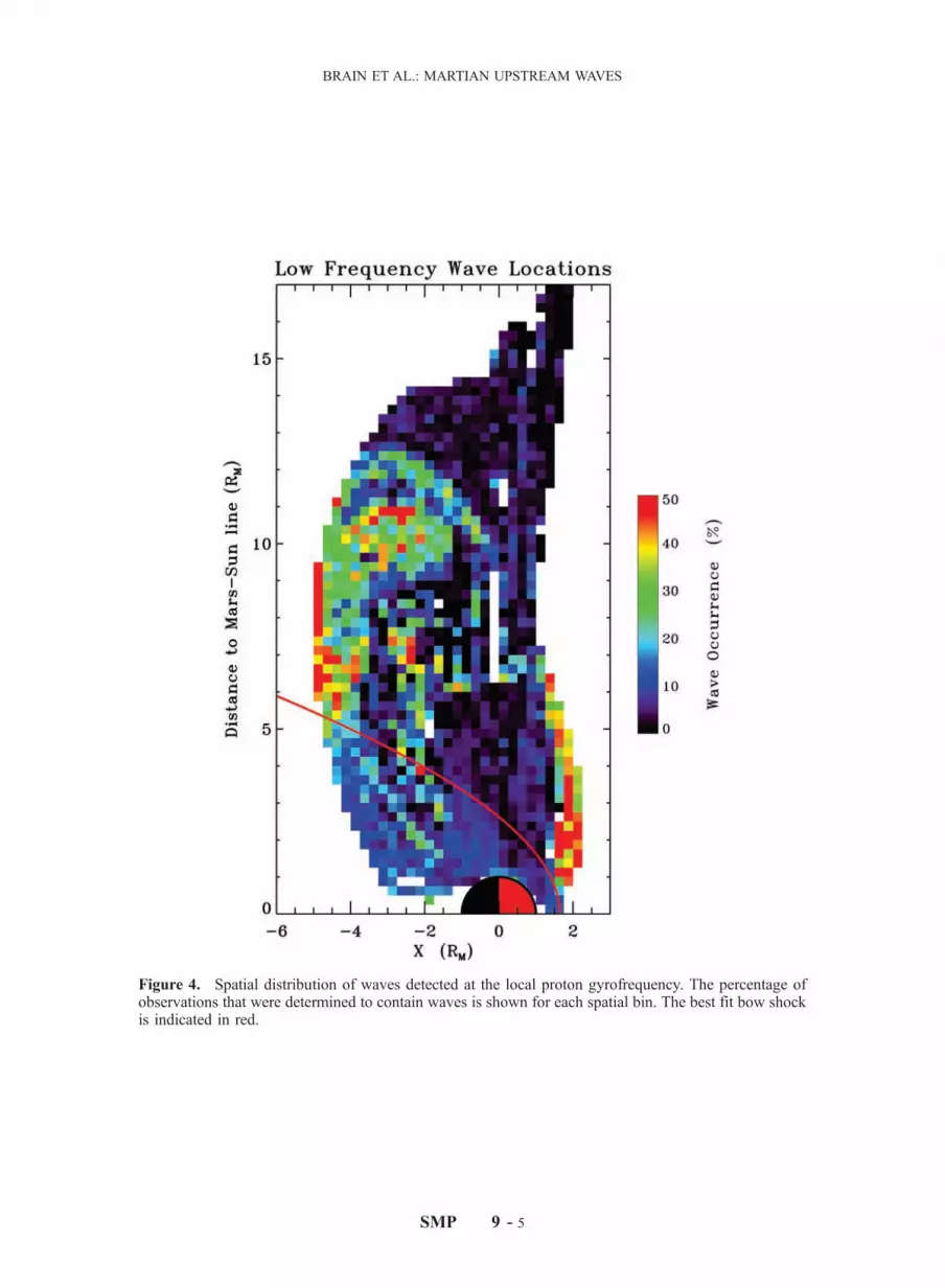
Figure 4. Spatial distribution of waves detected at the local proton gyrofrequency. The percentage ofobservations that were determined to contain waves is shown for each spatial bin. The best fit bow shockis indicated in red.

SMP 9 - 5


Figure 6. Spatial distribution of power at the local proton gyrofrequency. Average power is shown as afunction of location for the x component of magnetic field in mean-field coordinates. The best fit bowshock is indicated in black.

SMP 9 - 7


Documents

Observations of low-frequency electromagnetic plasma waves upstream from the Martian shock