Offshore and onshore ground-generation airborne wind ... - WES

Offshore and onshore ground-generation airborne wind energypower curve characterizationMarkus Sommerfeld1, Martin Dörenkämper2, Jochem De Schutter3, and Curran Crawford1

1Institute for Integrated Energy Systems, University of Victoria, British Columbia, Canada2Fraunhofer Institute for Wind Energy Systems, Oldenburg, Germany3Systems Control and Optimization Laboratory IMTEK, Freiburg, Germany

Correspondence: Markus Sommerfeld ([email protected])

Abstract.

Airborne wind energy systems (AWESs) aim to operate at altitudes well above conventional wind turbines (WTs) and har-

vest energy from stronger winds aloft. While multiple AWES concepts compete for entry into the market, this study focuses

on ground-generation AWES. Various companies and researchers proposed power curve characterizations for AWES, but no

consensus for an industry-wide standard has been reached. An universal description of a ground-generation AWES power5

curve is difficult to define because of complex tether and drag losses as well as alternating flight paths over changing wind

conditions with altitude, as compared to conventional WT with winds at fixed hub height and rotor area normalization. There-

fore, this study determines AWES power and annual energy prediction (AEP) based on the awebox optimal control model

for two AWES sizes, driven by representative 10-minute onshore and offshore mesoscale WRF wind data. The wind resource

is analyzed with respect to atmospheric stability as well as annual and diurnal variation. The wind data is categorized using10

k-means clustering, to reduce the computational cost. The impact of changing wind conditions on AWES trajectory and power

cycle is investigated. Optimal operating heights are below 400 m onshore and below 200 m offshore. Efforts are made to de-

rive AWES power coefficients similar to conventional WT to enable a simple power and AEP estimation for a given site and

system. This AWES power coefficient decreases up to rated power due to the increasing tether length with wind speed and the

accompanying tether losses. A comparison between different AEP estimation methods shows that a low number of clusters15

with three representative wind profiles within the clusters yields the highest AEP, as other wind models average out high wind

speeds which are responsible for a high percentage of the overall AEP.

1 Introduction

Airborne wind energy systems (AWESs) aspire to harvest stronger and less turbulent winds at mid-altitude, here defined as

heights above 100 m and below 1500 m, which are unreachable with conventional wind turbines (WTs). The prospects of20

higher energy yield combined with reduced capital cost motivate the development of this novel class of renewable energy

technology (Lunney et al., 2017; Fagiano and Milanese, 2012). Unlike conventional wind turbines, which have converged to a

single concept with three blades, nacelle and generator supported by a conical tower, several different AWES designs are under

investigation by numerous companies and research institutes (Cherubini et al., 2015). These kite-inspired systems consist of

1

https://doi.org/10.5194/wes-2020-120Preprint. Discussion started: 19 November 2020c© Author(s) 2020. CC BY 4.0 License.

three main components: a flying wing or kite, a ground station and a tether to connect them. Various concepts compete for entry25

into the market. This study focuses on the two-phase, ground-generation concept, also referred to as pumping-mode which is

the main route that industry is investigating. During the reel-out phase the wing pulls a non-conductive tether from a drum

which is connected to a generator, thereby producing electricity. During the reel-in phase the wing reduces its aerodynamic

forces by adjusting the angle of attack to reduce the power needed to pull the tether back in. Other concepts such as fly-gen,

aerostat or rotary lift are not within the scope of this study (Cherubini et al., 2015). Since this technology is still in an early30

stage, validation of results is difficult.

A standardized power curve definition would enable comparison between different AWES concepts and to conventional wind

turbines. Together with the site-specific wind resource, power curves help wind park planners and AWES device manufacturers

to estimate the annual energy production (AEP) and determine financial viability. As such this work supports the development

and implementation of this novel technology (Malz et al., 2020).35

The power of an AWES highly depends on the wind speed magnitude and profile shape (wind speed and direction variation

with height) which determines the power output as well as optimal operating altitude and trajectory. Simple wind profile ap-

proximations using logarithmic or exponential wind speed profiles, which are often erroneously applied beyond earths surface

layer (Optis et al., 2016), might approximate long-term average conditions, but can not capture the broad variation of profile

shapes (Emeis, 2018). They are therefore an inappropriate approximation to estimate instantaneous, diurnal and seasonal vari-40

ation in electrical power output. However, they are the standard in most AWES power estimation studies (e.g. (Leuthold et al.,

2018; Licitra et al., 2019; De Schutter et al., 2018; Aull et al., 2020)). AWES need to dynamically adapt their flight trajectory to

changing winds in order to optimize power production. Wind conditions are determined by environmental, location-dependent

conditions (e.g. surface roughness) and weather phenomena on a multitude of temporal and spatial scales, subject to diurnal and

seasonal patterns. They can be estimated from mesoscale numerical weather prediction models such as the weather research45

and forecasting model (WRF), which is well known for conventional WT siting applications (Salvação and Guedes Soares,

2018; Dörenkämper et al., 2020). These numerical simulations should be corrected for systematic errors using measurements

such as light detection and ranging (LiDAR) during site assessment and deployment. Results in this study are exclusively based

on WRF mesoscale simulations, since measuring wind conditions at mid-altitudes is difficult due to reduced data availability

(Sommerfeld et al., 2019a) and measurements are hard to find, proprietary or confidential. We compare AWES performance50

for an onshore location in northern Germany near the city of Pritzwalk (Sommerfeld et al., 2019b) and an offshore location at

the FINO3 research platform in the North Sea. WT and AWES performance using logarithmic wind profiles are compared as

reference.

Section 2 describes the onshore and offshore wind resource based on the WRF model. Sub-sections give a brief overview

of the WRF model and compare wind statistics. Section 3 introduces the k-means clustering algorithm and summarizes results55

of clustered wind velocity profiles (profiles of both longitudinal and lateral wind component). These include cluster averaged

profiles and correlation with seasonal, diurnal and atmospheric stability. Section 4.1 introduces the awebox optimization

framework. It summarizes aircraft, tether and ground station models as well as implemented constraints and initialization

used to derive the results shown in section 5. This includes flight paths and time series of various performance parameters,

2


a statistical analysis of tether length and operating altitude. Furthermore, we compare power curve characterization, capacity60

factor and AEP estimation. Based on these results, an AWES power coefficient is defined to approximate AWES efficiency and

power based on system size and wind speed. Finally, Section 6 concludes with an outlook and motivation for future work.

2 Wind data

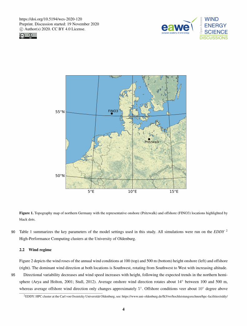
This study compares the AWES performance at two representative locations in Europe (see fig 1). “Onshore” wind data at

the Pritzwalk Sommersberg airport (lat: 53◦10′47.00′′N, lon: 12◦11′20.98′′E) in northern Germany and comprises 12 months65

of WRF simulation between September 2015 and September 2016. The area surrounding the airport mostly consists of flat

agricultural land with the town of Pritzwalk to the south and is therefore a fitting location for wind energy generation (See

(Sommerfeld et al., 2019a) and (Sommerfeld et al., 2019b) for details). The FINO3 research platform in the North Sea (lat:

55◦11,7′N, lon: 7◦9,5′ E) was chosen as a representative “offshore” location due to the proximity to several offshore wind

farms and the amount of comprehensive reference measurements (Peña et al., 2015). The offshore simulation covers the time70

frame between September 2013 and September 2014.

2.1 Mesoscale model

The mesoscale simulations in this study were carried out using the weather research and forecasting (WRF) model from

(Skamarock et al., 2008). The onshore simulation was performed with version 3.6.1 before the 2018 release of WRF version

4.0.2 1 in which the offshore simulations were computed. The setup of the model has been adapted and constantly optimized75

for wind energy applications by the authors in the framework of various projects and applications in recent years (Dörenkämper

et al., 2015, 2017; Dörenkämper et al., 2020; Hahmann et al., 2020; Sommerfeld et al., 2019c).

The focus of this study is not on the detailed comparison between mesoscale models, but on AWES performance subject to

representative onshore and offshore wind conditions determined based on clustered wind profiles (described on section 3). To

that end, both WRF models provide adequate wind data for our purposes. data Both simulations consist of three nested domains80

centered around either the FINO3 met mast (see Figure 1) or the Pritzwalk Sommersberg airport. Atmospheric boundary condi-

tions are defined by ERA-Interim (Dee et al., 2011) for the onshore location and by ERA5 (Hersbach and Dick, 2016) reanalysis

data for the offshore location, while sea surface parameters for the offshore location are based on OSTIA (Donlon et al., 2012).

These data sets have proven to provide good results for wind energy relevant heights and sites (Olauson, 2018; Hahmann

et al., 2020). Both simulations use the MYNN 2.5 level scheme for the planetary boundary layer (PBL) physics (Nakanishi85

and Niino, 2009). While the onshore simulation was performed in one 12 month simulations (01.09.2015 - 31.08.2016), the

offshore simulation period consisted of 410 days (30.08.2013 - 14.10.2014) that were split into 41 simulations of 10 days

each with an additional 24 h of spin-up time per run. The data from the mesoscale models’ sigma levels (terrain-following)

were transformed to the geometric heights using the post-processing methodology described in (Dörenkämper et al., 2020).

1WRF model releases: https://github.com/wrf-model/WRF/releases

3


FINO3

Pritzwalk

50°N

55°N

5°E 10°E 15°E

Figure 1. Topography map of northern Germany with the representative onshore (Pritzwalk) and offshore (FINO3) locations highlighted by

black dots.

Table 1 summarizes the key parameters of the model settings used in this study. All simulations were run on the EDDY 290

High-Performance Computing clusters at the University of Oldenburg.

2.2 Wind regime

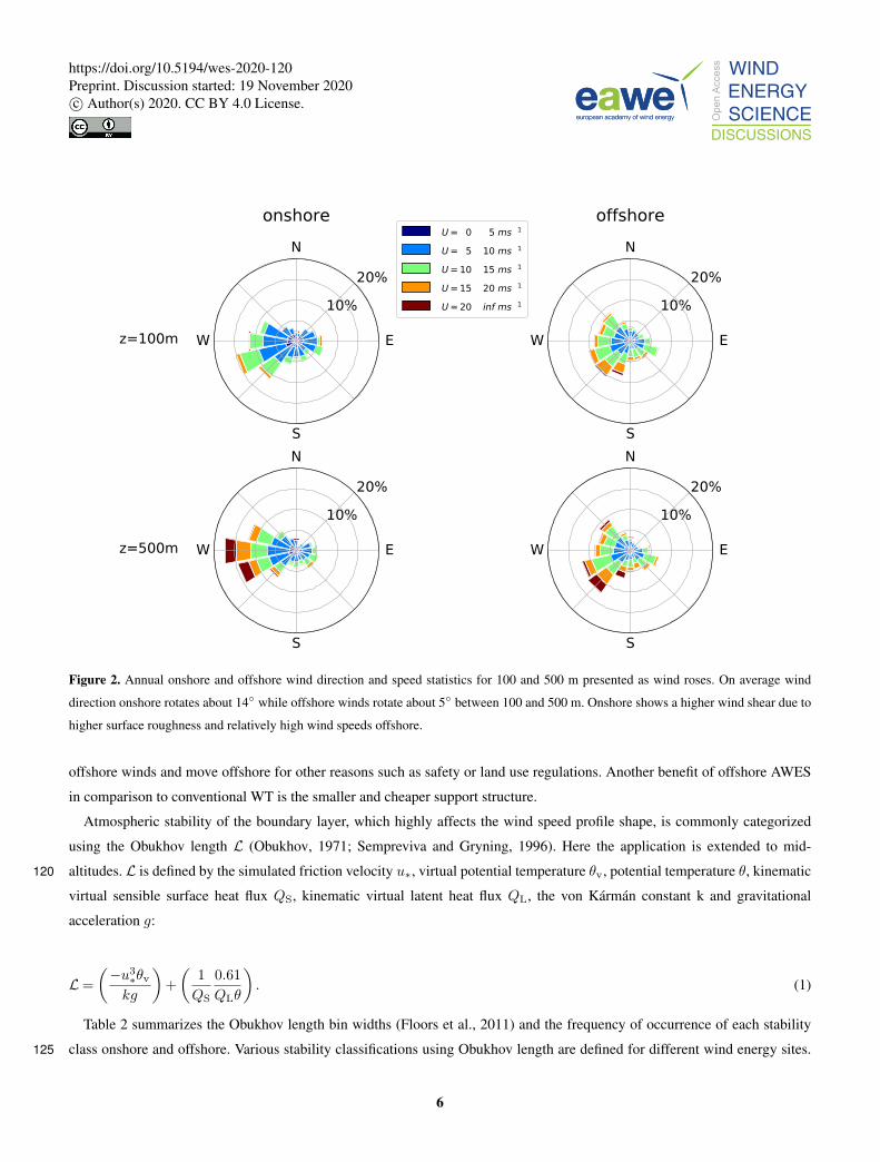
Figure 2 depicts the wind roses of the annual wind conditions at 100 (top) and 500 m (bottom) height onshore (left) and offshore

(right). The dominant wind direction at both locations is Southwest, rotating from Southwest to West with increasing altitude.

Directional variability decreases and wind speed increases with height, following the expected trends in the northern hemi-95

sphere (Arya and Holton, 2001; Stull, 2012). Average onshore wind direction rotates about 14◦ between 100 and 500 m,

whereas average offshore wind direction only changes approximately 5◦. Offshore conditions veer about 10◦ degree above

2EDDY: HPC cluster at the Carl von Ossietzky Universität Oldenburg, see: https://www.uni-oldenburg.de/fk5/wr/hochleistungsrechnen/hpc-facilities/eddy/

4


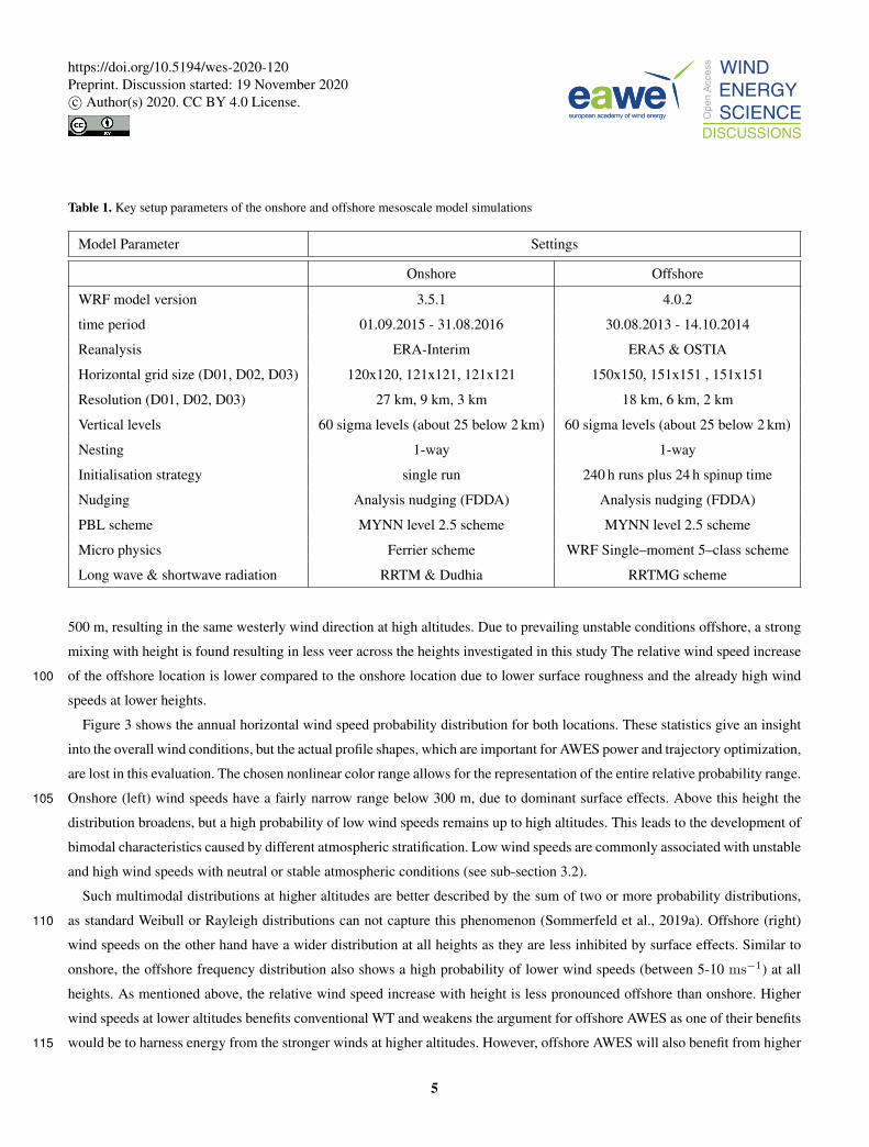
Table 1. Key setup parameters of the onshore and offshore mesoscale model simulations

Model Parameter Settings

Onshore Offshore

WRF model version 3.5.1 4.0.2

time period 01.09.2015 - 31.08.2016 30.08.2013 - 14.10.2014

Reanalysis ERA-Interim ERA5 & OSTIA

Horizontal grid size (D01, D02, D03) 120x120, 121x121, 121x121 150x150, 151x151 , 151x151

Resolution (D01, D02, D03) 27 km, 9 km, 3 km 18 km, 6 km, 2 km

Vertical levels 60 sigma levels (about 25 below 2 km) 60 sigma levels (about 25 below 2 km)

Nesting 1-way 1-way

Initialisation strategy single run 240 h runs plus 24 h spinup time

Nudging Analysis nudging (FDDA) Analysis nudging (FDDA)

PBL scheme MYNN level 2.5 scheme MYNN level 2.5 scheme

Micro physics Ferrier scheme WRF Single–moment 5–class scheme

Long wave & shortwave radiation RRTM & Dudhia RRTMG scheme

500 m, resulting in the same westerly wind direction at high altitudes. Due to prevailing unstable conditions offshore, a strong

mixing with height is found resulting in less veer across the heights investigated in this study The relative wind speed increase

of the offshore location is lower compared to the onshore location due to lower surface roughness and the already high wind100

speeds at lower heights.

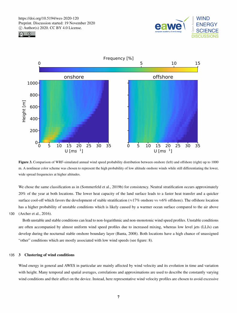
Figure 3 shows the annual horizontal wind speed probability distribution for both locations. These statistics give an insight

into the overall wind conditions, but the actual profile shapes, which are important for AWES power and trajectory optimization,

are lost in this evaluation. The chosen nonlinear color range allows for the representation of the entire relative probability range.

Onshore (left) wind speeds have a fairly narrow range below 300 m, due to dominant surface effects. Above this height the105

distribution broadens, but a high probability of low wind speeds remains up to high altitudes. This leads to the development of

bimodal characteristics caused by different atmospheric stratification. Low wind speeds are commonly associated with unstable

and high wind speeds with neutral or stable atmospheric conditions (see sub-section 3.2).

Such multimodal distributions at higher altitudes are better described by the sum of two or more probability distributions,

as standard Weibull or Rayleigh distributions can not capture this phenomenon (Sommerfeld et al., 2019a). Offshore (right)110

wind speeds on the other hand have a wider distribution at all heights as they are less inhibited by surface effects. Similar to

onshore, the offshore frequency distribution also shows a high probability of lower wind speeds (between 5-10 ms−1) at all

heights. As mentioned above, the relative wind speed increase with height is less pronounced offshore than onshore. Higher

wind speeds at lower altitudes benefits conventional WT and weakens the argument for offshore AWES as one of their benefits

would be to harness energy from the stronger winds at higher altitudes. However, offshore AWES will also benefit from higher115

5


E

N

W

S

10%20%

onshoreU= 0− 5 ms−1

U= 5−10 ms−1

U=10−15 ms−1

U=15−20 ms−1

U=20− inf ms−1

E

N

W

S

10%20%

E

N

W

S

10%20%

offshore

E

N

W

S

10%20%

z=100m

z=500m

Figure 2. Annual onshore and offshore wind direction and speed statistics for 100 and 500 m presented as wind roses. On average wind

direction onshore rotates about 14◦ while offshore winds rotate about 5◦ between 100 and 500 m. Onshore shows a higher wind shear due to

higher surface roughness and relatively high wind speeds offshore.

offshore winds and move offshore for other reasons such as safety or land use regulations. Another benefit of offshore AWES

in comparison to conventional WT is the smaller and cheaper support structure.

Atmospheric stability of the boundary layer, which highly affects the wind speed profile shape, is commonly categorized

using the Obukhov length L (Obukhov, 1971; Sempreviva and Gryning, 1996). Here the application is extended to mid-

altitudes. L is defined by the simulated friction velocity u∗, virtual potential temperature θv, potential temperature θ, kinematic120

virtual sensible surface heat flux QS, kinematic virtual latent heat flux QL, the von Kármán constant k and gravitational

acceleration g:

L=(−u3

∗θv

kg

)+(

1QS

0.61QLθ

). (1)

Table 2 summarizes the Obukhov length bin widths (Floors et al., 2011) and the frequency of occurrence of each stability

class onshore and offshore. Various stability classifications using Obukhov length are defined for different wind energy sites.125

6


0 5 10 15 20 25 30 35U [ms−1]

0

200

400

600

800

1000

Height [m

]

onshore

0 5 10 15 20 25 30 35U [ms−1]

offshore

0 5 10 15Frequency [%]

Figure 3. Comparison of WRF-simulated annual wind speed probability distribution between onshore (left) and offshore (right) up to 1000

m. A nonlinear color scheme was chosen to represent the high probability of low altitude onshore winds while still differentiating the lower,

wide spread frequencies at higher altitudes.

We chose the same classification as in (Sommerfeld et al., 2019b) for consistency. Neutral stratification occurs approximately

20% of the year at both locations. The lower heat capacity of the land surface leads to a faster heat transfer and a quicker

surface cool-off which favors the development of stable stratification (≈17% onshore vs ≈6% offshore). The offshore location

has a higher probability of unstable conditions which is likely caused by a warmer ocean surface compared to the air above

(Archer et al., 2016).130

Both unstable and stable conditions can lead to non-logarithmic and non-monotonic wind speed profiles. Unstable conditions

are often accompanied by almost uniform wind speed profiles due to increased mixing, whereas low level jets (LLJs) can

develop during the nocturnal stable onshore boundary layer (Banta, 2008). Both locations have a high chance of unassigned

“other” conditions which are mostly associated with low wind speeds (see figure: 8).

3 Clustering of wind conditions135

Wind energy in general and AWES in particular are mainly affected by wind velocity and its evolution in time and variation

with height. Many temporal and spatial averages, correlations and approximations are used to describe the constantly varying

wind conditions and their affect on the device. Instead, here representative wind velocity profiles are chosen to avoid excessive

7


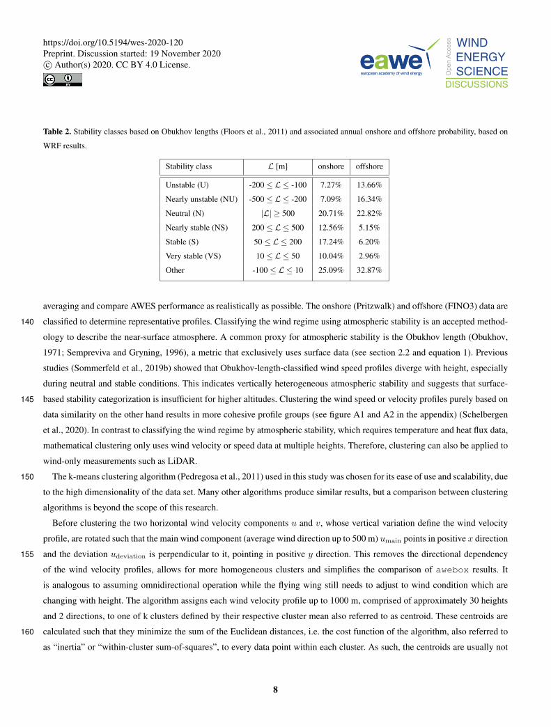
Table 2. Stability classes based on Obukhov lengths (Floors et al., 2011) and associated annual onshore and offshore probability, based on

WRF results.

Stability class L [m] onshore offshore

Unstable (U) -200 ≤ L≤ -100 7.27% 13.66%

Nearly unstable (NU) -500 ≤ L≤ -200 7.09% 16.34%

Neutral (N) |L| ≥ 500 20.71% 22.82%

Nearly stable (NS) 200 ≤ L≤ 500 12.56% 5.15%

Stable (S) 50 ≤ L≤ 200 17.24% 6.20%

Very stable (VS) 10 ≤ L≤ 50 10.04% 2.96%

Other -100 ≤ L≤ 10 25.09% 32.87%

averaging and compare AWES performance as realistically as possible. The onshore (Pritzwalk) and offshore (FINO3) data are

classified to determine representative profiles. Classifying the wind regime using atmospheric stability is an accepted method-140

ology to describe the near-surface atmosphere. A common proxy for atmospheric stability is the Obukhov length (Obukhov,

1971; Sempreviva and Gryning, 1996), a metric that exclusively uses surface data (see section 2.2 and equation 1). Previous

studies (Sommerfeld et al., 2019b) showed that Obukhov-length-classified wind speed profiles diverge with height, especially

during neutral and stable conditions. This indicates vertically heterogeneous atmospheric stability and suggests that surface-

based stability categorization is insufficient for higher altitudes. Clustering the wind speed or velocity profiles purely based on145

data similarity on the other hand results in more cohesive profile groups (see figure A1 and A2 in the appendix) (Schelbergen

et al., 2020). In contrast to classifying the wind regime by atmospheric stability, which requires temperature and heat flux data,

mathematical clustering only uses wind velocity or speed data at multiple heights. Therefore, clustering can also be applied to

wind-only measurements such as LiDAR.

The k-means clustering algorithm (Pedregosa et al., 2011) used in this study was chosen for its ease of use and scalability, due150

to the high dimensionality of the data set. Many other algorithms produce similar results, but a comparison between clustering

algorithms is beyond the scope of this research.

Before clustering the two horizontal wind velocity components u and v, whose vertical variation define the wind velocity

profile, are rotated such that the main wind component (average wind direction up to 500 m) umain points in positive x direction

and the deviation udeviation is perpendicular to it, pointing in positive y direction. This removes the directional dependency155

of the wind velocity profiles, allows for more homogeneous clusters and simplifies the comparison of awebox results. It

is analogous to assuming omnidirectional operation while the flying wing still needs to adjust to wind condition which are

changing with height. The algorithm assigns each wind velocity profile up to 1000 m, comprised of approximately 30 heights

and 2 directions, to one of k clusters defined by their respective cluster mean also referred to as centroid. These centroids are

calculated such that they minimize the sum of the Euclidean distances, i.e. the cost function of the algorithm, also referred to160

as “inertia” or “within-cluster sum-of-squares”, to every data point within each cluster. As such, the centroids are usually not

8


actual data points, but rather the average of that cluster. The resulting cluster labels are random results of initialization and are

therefore insignificant. Later evaluation uses clusters sorted by average wind speed up to 500 m.

The variable k refers to the fixed, predefined number of clusters. The choice of k significantly affects the accuracy of

the resulting power and AEP predictions (see section 5.5) as well as the computational cost associated with clustering (pre-165

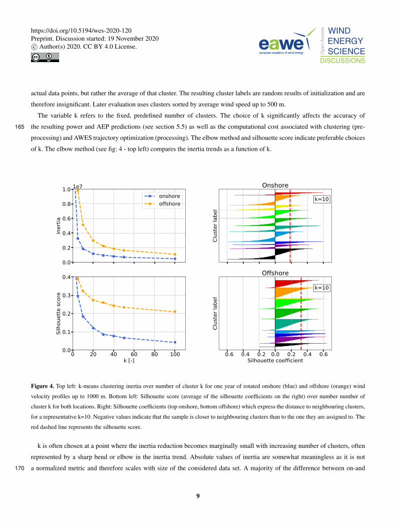
processing) and AWES trajectory optimization (processing). The elbow method and silhouette score indicate preferable choices

of k. The elbow method (see fig: 4 - top left) compares the inertia trends as a function of k.

0.0

0.2

0.4

0.6

0.8

1.0

inertia

1e7onshoreoffshore

Clus

ter lab

el

k=10

Onshore

0 20 40 60 80 100k [-]

0.0

0.1

0.2

0.3

0.4

Silhou

ette sc

ore

−0.6 −0.4 −0.2 0.0 0.2 0.4 0.6Silhouette coefficient

Clus

ter lab

el

k=10

Offshore

Figure 4. Top left: k-means clustering inertia over number of cluster k for one year of rotated onshore (blue) and offshore (orange) wind

velocity profiles up to 1000 m. Bottom left: Silhouette score (average of the silhouette coefficients on the right) over number number of

cluster k for both locations. Right: Silhouette coefficients (top onshore, bottom offshore) which express the distance to neighbouring clusters,

for a representative k=10. Negative values indicate that the sample is closer to neighbouring clusters than to the one they are assigned to. The

red dashed line represents the silhouette score.

k is often chosen at a point where the inertia reduction becomes marginally small with increasing number of clusters, often

represented by a sharp bend or elbow in the inertia trend. Absolute values of inertia are somewhat meaningless as it is not

a normalized metric and therefore scales with size of the considered data set. A majority of the difference between on-and170

9


offshore is likely due to different number of vertical grid cells which the algorithm interprets as dimensions (see table 1). The

silhouette coefficients on the other hand are normalized between -1 (worst) and 1 (best) and indicate the membership of a data

point to its cluster in comparison to other clusters. A negative value suggests that a data point is assigned to the wrong cluster.

The silhouette score is the average of all silhouette coefficients for a fixed number of clusters k. Its trend is shown in the bottom

left of figure 4 . The top right depicts the onshore and the bottom right the offshore silhouette coefficients for a representative175

k of 10. Note that the clusters are unsorted as a result of the random initialization process. Therefore, their labels (1 to 10) are

omitted. Silhouette coefficients and the resulting silhouette score illustrate that the offshore clusters are more coherent than the

onshore clusters. Onshore clusters also have more negative silhouette coefficients which could indicate too many or too few

clusters. Another possible explanation could be that the continuous nature of wind which results in a high cluster proximity as

well as the high variability of profile shapes onshore led to a worse score. The following sub-section shows that non-monotonic180

wind velocity profiles (e.g. profiles with low level jets (LLJs), which are more common onshore, intersect with other clusters

and therefore reduce the overall silhouette score.

3.1 Analysis of clustered profiles

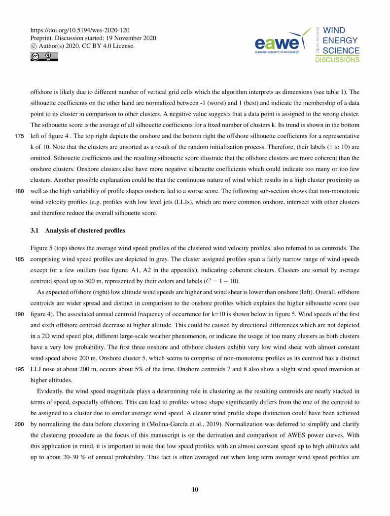
Figure 5 (top) shows the average wind speed profiles of the clustered wind velocity profiles, also referred to as centroids. The

comprising wind speed profiles are depicted in grey. The cluster assigned profiles span a fairly narrow range of wind speeds185

except for a few outliers (see figure: A1, A2 in the appendix), indicating coherent clusters. Clusters are sorted by average

centroid speed up to 500 m, represented by their colors and labels (C = 1− 10).

As expected offshore (right) low altitude wind speeds are higher and wind shear is lower than onshore (left). Overall, offshore

centroids are wider spread and distinct in comparison to the onshore profiles which explains the higher silhouette score (see

figure 4). The associated annual centroid frequency of occurrence for k=10 is shown below in figure 5. Wind speeds of the first190

and sixth offshore centroid decrease at higher altitude. This could be caused by directional differences which are not depicted

in a 2D wind speed plot, different large-scale weather phenomenon, or indicate the usage of too many clusters as both clusters

have a very low probability. The first three onshore and offshore clusters exhibit very low wind shear with almost constant

wind speed above 200 m. Onshore cluster 5, which seems to comprise of non-monotonic profiles as its centroid has a distinct

LLJ nose at about 200 m, occurs about 5% of the time. Onshore centroids 7 and 8 also show a slight wind speed inversion at195

higher altitudes.

Evidently, the wind speed magnitude plays a determining role in clustering as the resulting centroids are nearly stacked in

terms of speed, especially offshore. This can lead to profiles whose shape significantly differs from the one of the centroid to

be assigned to a cluster due to similar average wind speed. A clearer wind profile shape distinction could have been achieved

by normalizing the data before clustering it (Molina-García et al., 2019). Normalization was deferred to simplify and clarify200

the clustering procedure as the focus of this manuscript is on the derivation and comparison of AWES power curves. With

this application in mind, it is important to note that low speed profiles with an almost constant speed up to high altitudes add

up to about 20-30 % of annual probability. This fact is often averaged out when long term average wind speed profiles are

10


0 5 10 15 20 25 30 35U [ms−1]

0

200

400

600

800

1000

Height [m

]

onshore

0 5 10 15 20 25 30 35U [ms−1]

offshore

1 5 10C [-]

01020

f [%]

1 5 10C [-]

0 5 10 15 20 25U(z≤500m) [ms−1]

Figure 5. Onshore (left) and offshore (right) average annual wind speed profiles (or centroids) resulting from the k-means clustering process

for k = 10 over height (top). Comprising WRF simulated wind velocity profiles depicted in grey. Centroids are sorted, labeled and colored in

ascending order of average wind speed up to 500 m. The corresponding cluster frequency f for each cluster C is shown below.

considered. AWES therefore need to be able to either operate under such low speed conditions or be able to safely land and

take-off.205

3.2 Analysis of clustered statistics

Figures 6 to 8 summarize the correlation between representative clusters (k=10) and monthly, diurnal and atmospheric stability

for the onshore (top row) and offshore (bottom row) location. This reveals patterns within the data set and gives insight into

the wind prevailing regime. Clusters are sorted in ascending order of centroid average wind speed up to 500 m and colored

accordingly. The corresponding centroids are shown in figure 5.210

11


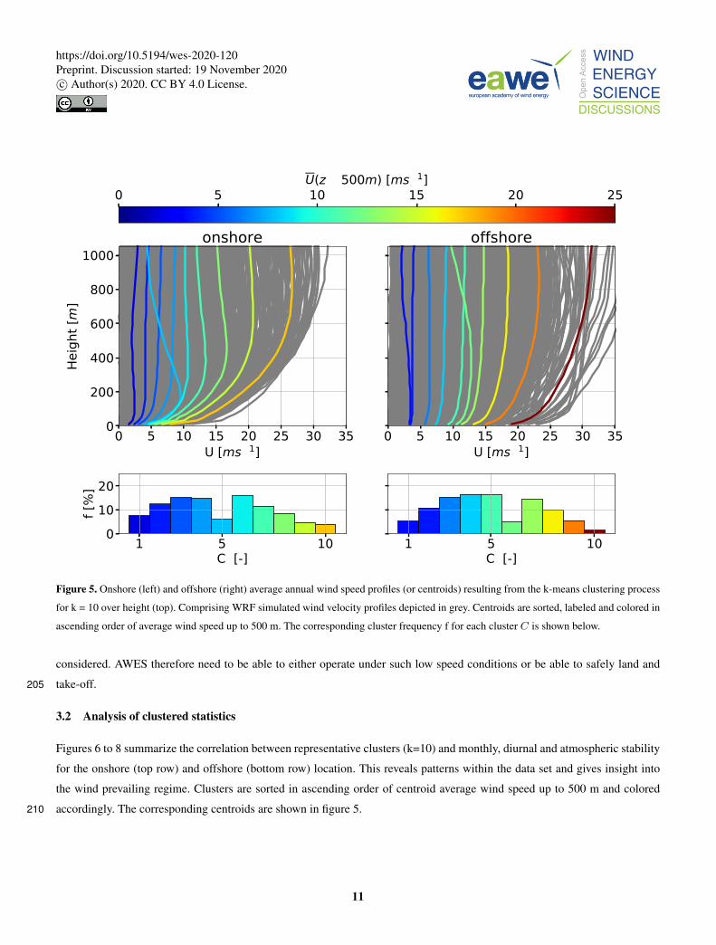
Both locations follow a distinct annual pattern (see figure 6) during which profiles associated with high wind speeds increase

during the winter months and profiles with low wind speeds are predominantly found in summer. The two onshore and offshore

clusters associated with the highest wind speed are almost exclusively present during November to February.

0

10

20

30

Onsh

ore

freq

uenc

y [%

]

Jan Feb Mar Apr May Jun Jul Aug Sep Oct Nov Dec

0

10

20

30

Offshore

fr

eque

ncy [%

]

0

5

10

15

20

25

U(z≤500m

) [ms−

1 ]

cluster label k=[1, 10]

Figure 6. Monthly frequency of k-means clustered onshore (top) and (offshore) wind velocity profiles for a representative k=10. Clusters are

sorted and colored by average wind speed up to 500 m. Centroids associated with each cluster can be found in figure 5.

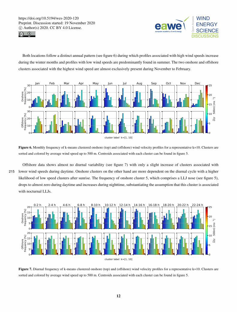
Offshore data shows almost no diurnal variability (see figure 7) with only a slight increase of clusters associated with

lower wind speeds during daytime. Onshore clusters on the other hand are more dependent on the diurnal cycle with a higher215

likelihood of low speed clusters after sunrise. The frequency of onshore cluster 5, which comprises a LLJ nose (see figure 5),

drops to almost zero during daytime and increases during nighttime, substantiating the assumption that this cluster is associated

with nocturnal LLJs.

0

5

10

15

20

Onshore

freq

uenc [%

]

0-2 h 2-4 h 4-6 h 6-8 h 8-10 h 10-12 h 12-14 h 14-16 h 16-18 h 18-20 h 20-22 h 22-24 h

0

5

10

15

20

Offsho

re

freq

uenc [%

]

0

5

10

15

20

25

U(z≤50

0m) [ms−

1 ]

cluster label k=[1, 10]

Figure 7. Diurnal frequency of k-means clustered onshore (top) and (offshore) wind velocity profiles for a representative k=10. Clusters are

sorted and colored by average wind speed up to 500 m. Centroids associated with each cluster can be found in figure 5.

12


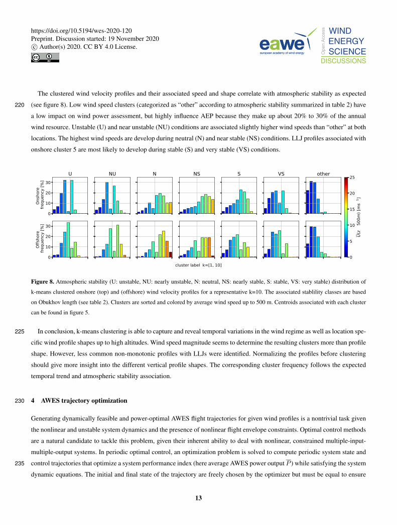
The clustered wind velocity profiles and their associated speed and shape correlate with atmospheric stability as expected

(see figure 8). Low wind speed clusters (categorized as “other” according to atmospheric stability summarized in table 2) have220

a low impact on wind power assessment, but highly influence AEP because they make up about 20% to 30% of the annual

wind resource. Unstable (U) and near unstable (NU) conditions are associated slightly higher wind speeds than “other” at both

locations. The highest wind speeds are develop during neutral (N) and near stable (NS) conditions. LLJ profiles associated with

onshore cluster 5 are most likely to develop during stable (S) and very stable (VS) conditions.

0

10

20

30

Onshore

freq ency [%

]

U NU N NS S VS other

0

10

20

30

Offshore

freq ency [%

]

0

5

10

15

20

25

U(z≤50

0m) [ms−

1 ]

cl ster label k=[1, 10]

Figure 8. Atmospheric stability (U: unstable, NU: nearly unstable, N: neutral, NS: nearly stable, S: stable, VS: very stable) distribution of

k-means clustered onshore (top) and (offshore) wind velocity profiles for a representative k=10. The associated stablility classes are based

on Obukhov length (see table 2). Clusters are sorted and colored by average wind speed up to 500 m. Centroids associated with each cluster

can be found in figure 5.

In conclusion, k-means clustering is able to capture and reveal temporal variations in the wind regime as well as location spe-225

cific wind profile shapes up to high altitudes. Wind speed magnitude seems to determine the resulting clusters more than profile

shape. However, less common non-monotonic profiles with LLJs were identified. Normalizing the profiles before clustering

should give more insight into the different vertical profile shapes. The corresponding cluster frequency follows the expected

temporal trend and atmospheric stability association.

4 AWES trajectory optimization230

Generating dynamically feasible and power-optimal AWES flight trajectories for given wind profiles is a nontrivial task given

the nonlinear and unstable system dynamics and the presence of nonlinear flight envelope constraints. Optimal control methods

are a natural candidate to tackle this problem, given their inherent ability to deal with nonlinear, constrained multiple-input-

multiple-output systems. In periodic optimal control, an optimization problem is solved to compute periodic system state and

control trajectories that optimize a system performance index (here average AWES power output P ) while satisfying the system235

dynamic equations. The initial and final state of the trajectory are freely chosen by the optimizer but must be equal to ensure

13


periodic operation. We here apply this methodology to generate realistic single-wing, ground-generation AWES power curves

and AEP estimation based on simulated wind velocity profiles using the awebox. Take-off and landing are not considered in

this paper. Instead only the trajectory during the production cycle is optimized.

4.1 Optimization model overview240

We consider a 6 degree of freedom (DOF) rigid-wing aircraft model. It uses pre-computed quadratic approximations of the

aerodynamic coefficients which are controlled via aileron, elevator and rudder deflection rates (Malz et al., 2019). The tether

is controlled by the tether jerk (...ltether) from which tether acceleration (l̈tether), speed (l̇tether = vtether) and length (ltether) are

derived. The tether is modeled as a single solid rod which can not be subjected to compressive forces (De Schutter et al., 2019).

The rod is divided into naero = 10 elements and tether drag is calculated individually for each element relative to apparent245

wind speed (Bronnenmeyer, 2018), with a tether drag coefficient of ctetherD = 1. Wind profiles are implemented as 2D wind

components rotated such that the main wind direction is in positive x direction and the deviation from it in y direction. This

is equivalent to assuming omnidirectional AWES operation with the wing still needing to adjust to changing wind conditions

with height. Furthermore, we include a simplified atmospheric model based on international standard atmosphere to account

for air density variation.250

4.2 Aircraft model

The aircraft aerodynamic coefficients are those available for the Ampyx AP2 (Malz et al., 2019; Ampyx) for comparison with

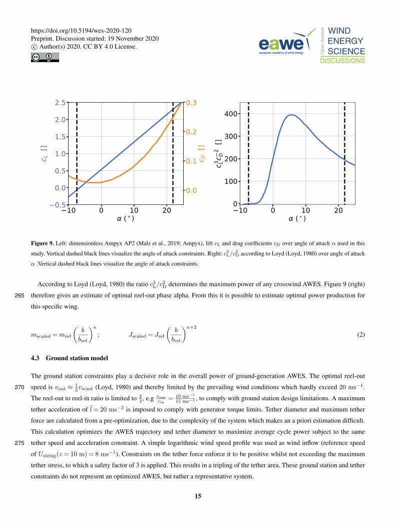
other publications and since no other AWES data were available3. Figure 9 (left) visualizes the implemented aircraft lift cL and

drag coefficient cD .

Lift is assumed to behave linearly in between the angle of attack constraints, visualized by black, vertical, dashed lines.255

Changes in the drag coefficient on the other hand are implemented by a quadratic approximation. This study compares two

aircraft sizes, one with a wing area of A= 20 m2 and another one with A= 50 m2. Aircraft geometry such as aspect ratio

is kept constant (AR= 10). The aircraft mass and inertia were scaled relative to wing span b (see equation 2), based on

the Galileo’s square–cube law. However, we chose a rather optimistic κ of 2 (pure geometric scaling would assume κ= 3),

assuming design and material improvements with scale. The wing loading of approximately 12.25 kgm−2 is consistent with260

the AP2 reference data. This results in an overestimation of output power and lower cut-in speed in comparison to a heavier

aircraft. The focus of this paper is on the derivation and investigation of the AWES power curve and not on realistic system

design which will be subject of a future paper on scaling study of AWES.

3other aerodynamic coefficients can be found under: https://github.com/awebox/awebox/blob/develop/awebox/opts/kite_data/ampyx_data.py

14


−10 0 10 20α ( ∘ ∘

−0.5

0.0

0.5

1.0

1.5

2.0

2.5

c L []

−10 0 10 20α ( ∘ ∘

0

100

200

300

400

c3 Lc−

2D

[]

0.0

0.1

0.2

0.3

c D []

Figure 9. Left: dimensionless Ampyx AP2 (Malz et al., 2019; Ampyx), lift cL and drag coefficients cD over angle of attack α used in this

study. Vertical dashed black lines visualize the angle of attack constraints. Right: c3L/c2D according to Loyd (Loyd, 1980) over angle of attack

α .Vertical dashed black lines visualize the angle of attack constraints.

According to Loyd (Loyd, 1980) the ratio c3L/c2D determines the maximum power of any crosswind AWES. Figure 9 (right)

therefore gives an estimate of optimal reel-out phase alpha. From this it is possible to estimate optimal power production for265

this specific wing.

mscaled =mref

(b

bref

)κ; Jscaled = Jref

(b

bref

)κ+2

(2)

4.3 Ground station model

The ground station constraints play a decisive role in the overall power of ground-generation AWES. The optimal reel-out

speed is vout ≈ 13vwind (Loyd, 1980) and thereby limited by the prevailing wind conditions which hardly exceed 20 ms−1.270

The reel-out to reel-in ratio is limited to 23 , e.g vout

vin= 10 ms−1

15 ms−1 , to comply with ground station design limitations. A maximum

tether acceleration of l̈ = 20 ms−2 is imposed to comply with generator torque limits. Tether diameter and maximum tether

force are calculated from a pre-optimization, due to the complexity of the system which makes an a priori estimation difficult.

This calculation optimizes the AWES trajectory and tether diameter to maximize average cycle power subject to the same

tether speed and acceleration constraint. A simple logarithmic wind speed profile was used as wind inflow (reference speed275

of Usizing(z = 10 m) = 8 ms−1). Constraints on the tether force enforce it to be positive whilst not exceeding the maximum

tether stress, to which a safety factor of 3 is applied. This results in a tripling of the tether area. These ground station and tether

constraints do not represent an optimized AWES, but rather a representative system.

15


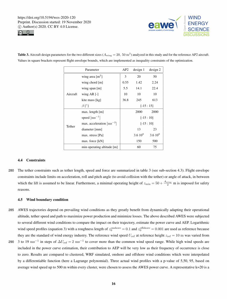
Table 3. Aircraft design parameters for the two different sizes (Awing = 20, 50 m2) analyzed in this study and for the reference AP2 aircraft.

Values in square brackets represent flight envelope bounds, which are implemented as inequality constraints of the optimization.

Parameter AP2 design 1 design 2

Aircraft

wing area [m2] 3 20 50

wing chord [m] 0.55 1.42 2.24

wing span [m] 5.5 14.1 22.4

wing AR [-] 10 10 10

kite mass [kg] 36.8 245 613

β [◦] [-15 : 15]

Tether

max. length [m] 2000 2000

speed [ms−1] [-15 : 10]

max. acceleration [ms−2] [-15 : 10]

diameter [mm] 13 23

max. stress [Pa] 3.6 109 3.6 109

max. force [kN] 150 500

min operating altitude [m] 60 75

4.4 Constraints

The tether constraints such as tether length, speed and force are summarized in table 3 (see sub-section 4.3). Flight envelope280

constraints include limits on acceleration, roll and pitch angle (to avoid collision with the tether) or angle of attack, in between

which the lift is assumed to be linear. Furthermore, a minimal operating height of zmin = 50 + Awing2 m is imposed for safety

reasons.

4.5 Wind boundary condition

AWES trajectories depend on prevailing wind conditions as they greatly benefit from dynamically adapting their operational285

altitude, tether speed and path to maximize power production and minimize losses. The above described AWES were subjected

to several different wind conditions to compare the impact on their trajectory, estimate the power curve and AEP. Logarithmic

wind speed profiles (equation 3) with a roughness length of zonshore0 = 0.1 and zoffshore

0 = 0.001 are used as reference because

they are the standard of wind energy industry. The reference wind speed Uref at reference height zref = 10 m was varied from

3 to 19 ms−1 in steps of ∆Uref = 2 ms−1 to cover more than the common wind speed range. While high wind speeds are290

included in the power curve estimation, their contribution to AEP will be very low as their frequency of occurrence is close

to zero. Results are compared to clustered, WRF simulated, onshore and offshore wind conditions which were interpolated

by a differentiable function (here a Lagrange polynomial). Three actual wind profiles with a p-value of 5,50, 95, based on

average wind speed up to 500 m within every cluster, were chosen to assess the AWES power curve. A representative k=20 is a

16


reasonable choice according to the elbow method and silhouette score described in section 3. To estimate AEP, cluster centroids295

across the range of k = 5− 100 were implemented. Wind conditions for the AEP estimation are based on the cluster centroids

for k = 5− 100 due to the high computational cost of running multiple profiles per cluster. These results are compared to the

AEP calculated from power of k=20 p5, p50 and p95 wind profiles.

Ulog = Uref

(log10(z/z0)

log10(zref/z0)

)(3)

4.6 Problem formulation and solution300

AWES trajectory optimization is a highly nonlinear and non-convex problem which likely has multiple local optima. Therefore,

the particular results generated by a numerical optimization solver can only guaranty local optimally, and usually depend on

the chosen initialization. This can result in unwanted or unrealistic AWES trajectories, which implies that the quality of all

solutions needs to be evaluated a posteriori.

A periodic optimal control problem is formulated to maximize the average cycle power (P ) of a single AWES subject to305

equality and in-equality constraints described above (De Schutter et al., 2019; Leuthold et al., 2018). The trajectory optimiza-

tion problem is discretized into 100 intervals using direct collocation.An initial guess is generated using a homotopy technique

similar to (Gros et al., 2013) with an estimated circular trajectory based on a fixed number of loops (here nloop = 4) at a 30◦

elevation angle and an estimated aircraft speed. The homotopy technique initially fully relaxes the dynamic constraints using

fictitious forces and moments to reduce model nonlinearity and coupling, improving the convergence of Newton-type opti-310

mization techniques. The constraints are then gradually re-introduced until the relaxed problem matches the original problem.

The resulting nonlinear program (NLP) is formulated in the symbolic modeling framework CasADi for Python (Andersson

et al., 2012) and solved using the linear solver MA57 (HSL) in IPOPT (Wächter and Biegler, 2006).

5 Results

In this section we compare representative onshore (Pritzwalk) and offshore (FINO3) trajectories and time series trends. Build-315

ing on that onshore and offshore operating height statistics and tether length trends are examined. AWES power curves are

determined based on average cycle power and wind speeds at different reference heights. From these power curve trends we

determine an AWES power coefficient cAWESp similar to conventional WT to allow for a quick estimate of AWES power based

on wing area, path length and wind speed. Lastly, the annual energy production (AEP) and capacity factor (cf) estimates of

different number of clusters are compared to Rayleigh distributed log-profiles as they are defined by IEC standards.320

5.1 Flight trajectory and time series results

This sub-section offers insight into typical optimized AWES flight trajectories. Figures 10 and A3 (appendix) compare the

trajectories of representative (chosen because of different wind speeds and profile shape) onshore and offshore profiles for an

17


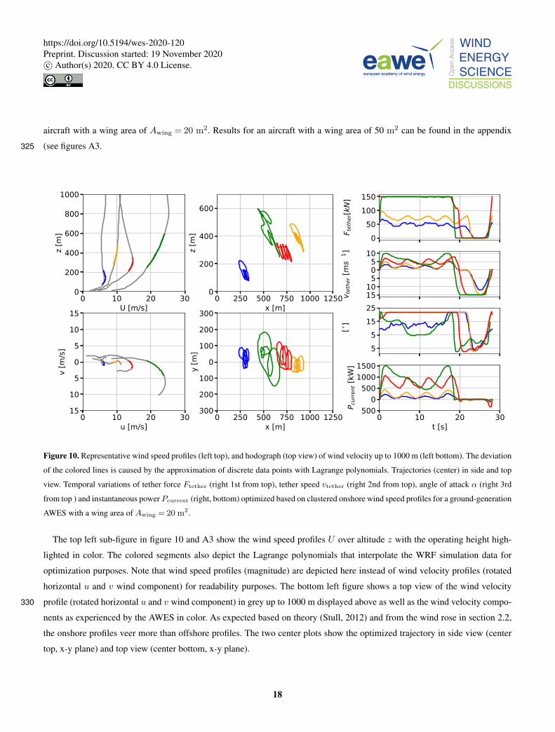
aircraft with a wing area of Awing = 20 m2. Results for an aircraft with a wing area of 50 m2 can be found in the appendix

(see figures A3.325

0 10 20 30U [m/s]

0

200

400

600

800

1000

z [m]

0 250 500 750 1000 1250x [m]

0

200

400

600

z [m]

0 250 500 750 1000 1250x [m]

−300

−200

−100

0

100

200

300

y [m

]

050

100150

F tethe

r[kN]

−15−10−505

10

v tethe

r [ms−

1 ]−55

1525

α [∘]

0 10 20 30t [s]

−5000

50010001500

P current [k

∘]

0 10 20 30u [m/s]

−15

−10

−5

0

5

10

15

v [m

/s]

Figure 10. Representative wind speed profiles (left top), and hodograph (top view) of wind velocity up to 1000 m (left bottom). The deviation

of the colored lines is caused by the approximation of discrete data points with Lagrange polynomials. Trajectories (center) in side and top

view. Temporal variations of tether force Ftether (right 1st from top), tether speed vtether (right 2nd from top), angle of attack α (right 3rd

from top ) and instantaneous power Pcurrent (right, bottom) optimized based on clustered onshore wind speed profiles for a ground-generation

AWES with a wing area of Awing = 20 m2.

The top left sub-figure in figure 10 and A3 show the wind speed profiles U over altitude z with the operating height high-

lighted in color. The colored segments also depict the Lagrange polynomials that interpolate the WRF simulation data for

optimization purposes. Note that wind speed profiles (magnitude) are depicted here instead of wind velocity profiles (rotated

horizontal u and v wind component) for readability purposes. The bottom left figure shows a top view of the wind velocity

profile (rotated horizontal u and v wind component) in grey up to 1000 m displayed above as well as the wind velocity compo-330

nents as experienced by the AWES in color. As expected based on theory (Stull, 2012) and from the wind rose in section 2.2,

the onshore profiles veer more than offshore profiles. The two center plots show the optimized trajectory in side view (center

top, x-y plane) and top view (center bottom, x-y plane).

18


When maximum tether force is reached the system starts to de-power while maintaining the same high tension (right, 1st

from top in figures 10 and A3). Such trajectories often extend perpendicular to the main wind direction (y-direction). This often335

results in odd and unrealistic or unexpected trajectories, even though these local minima are within the system constraints (roll

rate etc.). De-powering by increasing the elevation angle is also possible and likely to happen, but harder to determine as it is

not easily identifiable whether the elevation angle increased due to better wind conditions or to de-power the wing. Reducing

the angle of attack (right, 3rd from top) while maintaining constant maximum tether force (right, 1st from top) can be observed

in the highest onshore wind speed trajectory (green). The exact reason why the angle of attack at almost all wind speeds is340

lower offshore than onshore is hard to determine. A possible reason could be that the wind conditions offshore are so beneficial

that the system can operate at lower altitudes and therefore closer to optimal directly down wind conditions with optimal c3L/c2D

at around α≈ 8◦ predicted in figure 9. Onshore conditions on the other hand do not seem to allow for angle of attack close to

this optimal.

The algorithm seems to always maximize tether force and vary tether speed (right 2nd from top) close to optimal reel-out345

speed (vout ≈ 13vwind (Loyd, 1980)) to maximize average cycle power. At high wind speed the tether speed constraint is active

during the reel-in phase, presumably to keep this phase as short as possible. In these cases the trajectory starts to differ from

its predefined shape with distinct loops to de-power, visible in the power development during the production phase (green).

Trajectories for such high speed wind conditions without a tether force constraint, where the tether diameter is adjusted to

the wind conditions, would be closer to the looping paths seen for lower wind speeds (blue, orange, red). The time history of350

instantaneous power (Pcurrent; right bottom) clearly distinguishes the production and consumption phase of pumping-mode

(ground-generation) AWES. However, all optimized trajectories have a close to zero power usage during reel-in as they reduce

the angle of attack to near zero lift conditions. One commonality between all time series is that they all almost have the same

flight time independent of location, wind speed or aircraft size. The flight time is almost solely determined by the initial number

of loops, here five, used in the initialization procedure. Based on previous analyses, mechanical AWES power output seems to355

be insensitive to number of loops and flight time.

5.2 Tether length and altitude

This sub-section compares tether lengths and operating altitudes for onshore and offshore wind conditions for a wing size of

Awing = 20 m2. Results for the Awing = 50 m2 design can be found in the appendix in figure A6. The data is based on the

p5,p50, p95-th wind profiles of k=20 onshore and offshore clusters (see sub-section 4.5).360

Figure 11 (left) illustrates the minimum (blue) and maximum (orange) tether length ltether over reference wind speed, here

U(zref = 200 m), for both onshore (top) and offshore (bottom). The right side of the figure shows the frequency distribution

of operating altitude zoperating, calculated based on the trajectories described above in sub-section 5.1. Neither of the opti-

mizations reaches the maximum tether length of lmaxtether = 2000 m. Comparing both locations two very different trends emerge.

Onshore tethers are generally longer as operating altitudes tend to be higher due to higher wind shear and typically higher winds365

offshore. Where a tether length of approximately 600 m suffices for the entire offshore wind regime, onshore tethers need to be

at least 1000 m long, except for a few outliers which would benefit from an even longer tether. The gradual increase of tether

19


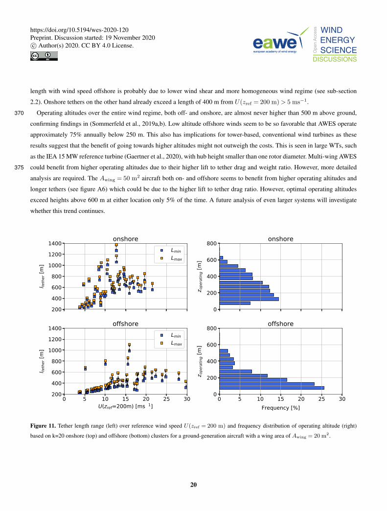
length with wind speed offshore is probably due to lower wind shear and more homogeneous wind regime (see sub-section

2.2). Onshore tethers on the other hand already exceed a length of 400 m from U(zref = 200 m)> 5 ms−1.

Operating altitudes over the entire wind regime, both off- and onshore, are almost never higher than 500 m above ground,370

confirming findings in (Sommerfeld et al., 2019a,b). Low altitude offshore winds seem to be so favorable that AWES operate

approximately 75% annually below 250 m. This also has implications for tower-based, conventional wind turbines as these

results suggest that the benefit of going towards higher altitudes might not outweigh the costs. This is seen in large WTs, such

as the IEA 15 MW reference turbine (Gaertner et al., 2020), with hub height smaller than one rotor diameter. Multi-wing AWES

could benefit from higher operating altitudes due to their higher lift to tether drag and weight ratio. However, more detailed375

analysis are required. The Awing = 50 m2 aircraft both on- and offshore seems to benefit from higher operating altitudes and

longer tethers (see figure A6) which could be due to the higher lift to tether drag ratio. However, optimal operating altitudes

exceed heights above 600 m at either location only 5% of the time. A future analysis of even larger systems will investigate

whether this trend continues.

200400600800

100012001400

l tether [m

]

onshoreLmin

Lmax

0

200

400

600

800

z ope

ratin

g [m]

onshore

0 5 10 15 20 25 30U(zref=200m) [ms−1]

200400600800

100012001400

l tether [m

]

offshoreLmin

Lmax

0 5 10 15 20 25 30Frequency [%]

0

200

400

600

800

z ope

ratin

g [m]

offshore

Figure 11. Tether length range (left) over reference wind speed U(zref = 200 m) and frequency distribution of operating altitude (right)

based on k=20 onshore (top) and offshore (bottom) clusters for a ground-generation aircraft with a wing area of Awing = 20 m2.

20


5.3 Power curve380

This sub-section compares AWES power curve representations based on various wind profile inputs over different reference

heights. Clustered WRF profiles are compared to logarithmic wind speed profiles, as defined in the IEC standards (International

Electrotechnical Commission, 2010). Due to many conceptually different AWES designs and the novelty of the technology,

there is no unanimously accepted AWES power curve definition. Therefore, no standard reference wind speed, equivalent to

wind speed at hub height for conventional WT, has been agreed upon. Similarly, no standard wind speed probability distribution385

such as the Rayleigh or Weibull distribution for conventional wind has been defined. Determining these parameters is more

complex than for conventional wind turbines as AWES power is highly dependents on the wind speed variation with height

and the resulting flight trajectories.

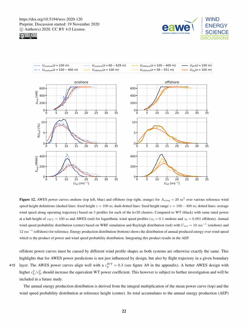
The power curves shown in figures 12 (Awing = 20 m2) and A8 (Awing = 50 m2) compare the cycle-average, onshore

(left,blue) and offshore (right, orange) power based on 60 different wind velocity profiles within k=20 clusters for wing areas390

of 20 and 50 m2, respectively. The dashed lines are curves based on a fixed reference height of z = 100 m. The dash-dotted

lines use the average wind speed between z = 100 m and z = 400 m and the the dotted lines use the average wind speed

over the respective AWES operating altitude. AWES power curves for logarithmic wind speed profiles with z0 = 0.1 (onshore,

left) and z0 = 0.001 (offshore, right) (Burton, 2011) as well as results using a simple WT power estimation (red) with a fixed

cWTp = 0.45 (see equation: 4) are depicted as reference. Air density ρair is calculated as a function of altitude z from a linear395

approximation of the standard atmosphere (Champion et al., 1985) (ρair(z) = 1.225 kgm−3− 0.00011 kgm−4 z). The Hub

height zWT is assumed to be 100 m for both onshore and offshore WT. The swept area of the turbine AWT is chosen such that

its rated power is equivalent to the AWES using:

PWT = cWTp

12ρairAWTU(zWT = 100 m) (4)

Cut-in and cut-out wind speeds were not used for either the AWES or WT to not limit specific designs. Therefore, energy400

production (bottom) is limited by the wind speed probability distribution (center). Wind statistics for the logarithmic wind speed

profiles are based on the IEC standard Rayleigh distribution (International Electrotechnical Commission, 2010) with a reference

wind speed of Uonshoreave = 10 ms−1 and Uoffshore

ave = 12 ms−1. The presented AWES and WT start producing significant power

around U ≈ 5 ms−1 and reach rated power between U 12 and 15 ms−1 at their respective reference heights. Whereas the

onshore power curve with a fixed reference height of 100 m aligns with the power curve of a conventional wind turbine, other405

power curves are seemingly below that. This is probably because of high wind shear profiles which lead to faster winds aloft

and higher operating altitudes with lower wind speeds at 100 m. The lower reference wind speeds, i.e. wind speeds at lower

altitudes, result in a power curve shift towards lower wind speeds (to the left). Offshore winds however experience less shear

(see sub-section : 2.2), which is why offshore AWES power curves for any reference height overlap with each other. Therefore,

a reference height of 200 m is likely a better choice as it results in smoother power curve. The divergence between WT and410

AWES power curves is likely caused by the reduction in AWES power coefficient cAWESp with wind speed (see sub-section

5.4) due to increased tether length and associated losses such as tether weight and drag. The difference between onshore and

21


0 5 10 15 20 25 30 350

200

400

600

p avg

[kW

]

onshore

Uonshore(z = 100 m)Uonshore(z = 100 400 m)

Uonshore(z = 60 629 m)Uoffshore(z = 100 m)

Uoffshore(z = 100 400 m)Uoffshore(z = 59 551 m)

UWT(z = 100 m)Ulog(z = 100 m)

0 5 10 15 20 25 30 350

200

400

600offshore

0 5 10 15 20 25 30 350

5

10

f(Ure

f) [%

]

0 5 10 15 20 25 30 350

5

10

0 5 10 15 20 25 30 35Uref [ms 1]

0

200

400

E avg

[MW

h]

0 5 10 15 20 25 30 35Uref [ms 1]

0

200

400

Figure 12. AWES power curves onshore (top left, blue) and offshore (top right, orange) for Awing = 20 m2 over various reference wind

speed height definitions (dashed lines: fixed height z = 100 m; dash-dotted lines: fixed height range z = 100−400 m; dotted lines: average

wind speed along operating trajectory) based on 3 profiles for each of the k=20 clusters. Compared to WT (black) with same rated power

at a hub height of zWT = 100 m and AWES (red) for logarithmic wind speed profiles (z0 = 0.1 onshore and z0 = 0.001 offshore). Annual

wind speed probability distribution (center) based on WRF simulation and Rayleigh distribution (red) with Uave = 10 ms−1 (onshore) and

12 ms−1 (offshore) for reference. Energy production distribution (bottom) shows the distribution of annual produced energy over wind speed

which is the product of power and wind speed probability distribution. Integrating this product results in the AEP.

offshore power curves must be caused by different wind profile shapes as both systems are otherwise exactly the same. This

highlights that for AWES power predictions is not just influenced by design, but also by flight trajectory in a given boundary

layer. The AWES power curves align well with a cWTp = 0.3 (see figure A9 in the appendix). A better AWES design with415

higher c3L/c2D should increase the equivalent WT power coefficient. This however is subject to further investigation and will be

included in a future study.

The annual energy production distribution is derived from the integral multiplication of the mean power curve (top) and the

wind speed probability distribution at reference height (center). Its total accumulates to the annual energy production (AEP)

22


further described in sub-section 5.5. AWES energy production distribution shifts towards higher wind speeds due to higher420

operating heights and their higher wind speeds. Similarly, the maximum onshore wind speed at 100 m is lower than offshore,

while wind speeds at other reference heights are similar to offshore.

Table 4 compiles the AEP of both system sizes and both locations. The table also includes the estimated WT AEP for

reference. Overall energy estimates for one system size and location are fairly consistent with each other. However, energy

estimates of the larger wing (Awing = 50 m2) onshore shows more variability due to the wider range of wind conditions and425

operating heights. This indicates that this effect scales with system size which will be investigated further in a future study.

The smaller AWES with a wing area of Awing = 20 m2 outperforms the WT with the same rated power onshore, whereas

the larger wing does not. This indicates that onshore wind conditions favor higher operating altitude due to higher wind

shear. Furthermore, the relative reduction in AWES energy with size could be related to additional losses associated with a

longer tether and heavier aircraft. Offshore, the WTs outperform the AWESs for both sizes as the lower wind shear favors430

lower operating altitudes. The offshore AEP is about 25 % larger than onshore for both AWES sizes, while WT performance

increases about 50% offshore in comparison to onshore due to better wind resource. This main difference between WT and

AWES can be explained by the high cWTp = 0.45 while the wind turbine equivalent of AWES power is closer to cWT

p = 0.3.

We assume that the best reference wind speed would be the wind speed along the actual AWES trajectory. Since this is hard

to estimate before site selection, a better reference wind speed would be calculated from the average between 100 and 600 m435

since this is the height at which most onshore and offshore AWES operate (see figure 11). Choosing one fixed reference height

might be an inadequate choice as larger AWES sweep a larger altitude range.

23


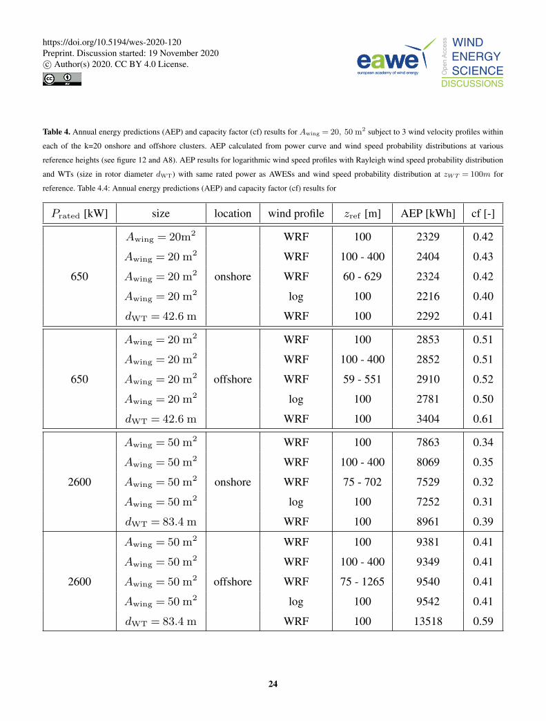
Table 4. Annual energy predictions (AEP) and capacity factor (cf) results for Awing = 20, 50 m2 subject to 3 wind velocity profiles within

each of the k=20 onshore and offshore clusters. AEP calculated from power curve and wind speed probability distributions at various

reference heights (see figure 12 and A8). AEP results for logarithmic wind speed profiles with Rayleigh wind speed probability distribution

and WTs (size in rotor diameter dWT) with same rated power as AWESs and wind speed probability distribution at zWT = 100m for

reference. Table 4.4: Annual energy predictions (AEP) and capacity factor (cf) results for

Prated [kW] size location wind profile zref [m] AEP [kWh] cf [-]

650

Awing = 20m2

onshore

WRF 100 2329 0.42

Awing = 20 m2 WRF 100 - 400 2404 0.43

Awing = 20 m2 WRF 60 - 629 2324 0.42

Awing = 20 m2 log 100 2216 0.40

dWT = 42.6 m WRF 100 2292 0.41

650

Awing = 20 m2

offshore

WRF 100 2853 0.51

Awing = 20 m2 WRF 100 - 400 2852 0.51

Awing = 20 m2 WRF 59 - 551 2910 0.52

Awing = 20 m2 log 100 2781 0.50

dWT = 42.6 m WRF 100 3404 0.61

2600

Awing = 50 m2

onshore

WRF 100 7863 0.34

Awing = 50 m2 WRF 100 - 400 8069 0.35

Awing = 50 m2 WRF 75 - 702 7529 0.32

Awing = 50 m2 log 100 7252 0.31

dWT = 83.4 m WRF 100 8961 0.39

2600

Awing = 50 m2

offshore

WRF 100 9381 0.41

Awing = 50 m2 WRF 100 - 400 9349 0.41

Awing = 50 m2 WRF 75 - 1265 9540 0.41

Awing = 50 m2 log 100 9542 0.41

dWT = 83.4 m WRF 100 13518 0.59

24


5.4 AWES power coefficient

To simplify the AWES power estimation, we derive the power coefficient for AWES cAWESp similar to conventional WT from

equation 5. The reference area is calculated from the swept area Aswept along the traveled path length lpath and wing span b440

(see table 3). The equation uses the wind speed U along the path and the average cycle power P . Air density ρair is calculated

from the linear approximation described in sub-section 5.3.

cp =P

ρair2 AsweptU3

(5)

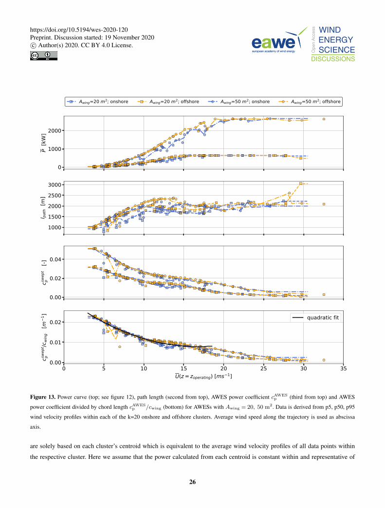
Figure 13 shows the previously described power curve (top) over average wind speed along the path U(zoperating). Data

points are based on awebox optimizations for wing areas of 20 and 50 m2 with three wind velocity profiles (p-value of 5,50,445

95 within each cluster) within each of the k=20 clusters. Onshore and offshore power curves of the same system size are close

to each other, however onshore power is slightly lower due to unfavorable wind conditions.

Similarly, the onshore path length (second from top) is generally smaller than offshore. Before reaching rated power, the

onshore path length for Awing = 20 m2 is approximately 18% smaller than the length of Awing = 50 m2; offshore this ratio

is only 12%. third sub-figure from the top shows the power coefficient cAWESp , which is calculated from equation 5, for two450

different AWES sizes at both locations. cAWESp is location and wind velocity profile independent as the reference wind speed

on the abscissa is the average speed along the trajectory. The difference between sizes amounts to the chord cwing, which scaled

with wing size since the aspect ratio AR= 10 of the wing is kept constant. A possible explanation for this difference is that

the mechanical power of a ground-generation AWES is the product of tether force and tether speed. Tether force scales with

wing area and tether speed increases because the tether length increases while the total cycle time remains almost constant (see455

sub-section 5.1 and 5.2). The decrease in cAWESp can be attributed to increased losses associated with a longer tether, i.e. tether

drag and weight. The bottom sub-figure depicts the scaled AWES power coefficient cAWESp /cwing which shows a nonlinear,

but consistent trend for all AWESs. A quadratic fit of cAWESp /cwing between cut-in and rated power (black line), described by:

cfitp

cwing= 0.00096 U(zoperating)2− 0.00308 U(zoperating) + 0.03286 (6)

is in good agreement with the data.460

5.5 AEP

This sub-section contrasts annual energy predictions (AEPs) and capacity factor (cf) based on the various power estimates and

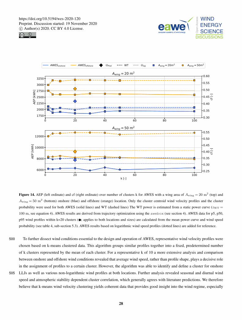
wind statistics. Figure 14 compares results for an increasing number of clusters (k= 2,5,10, 20, 30, 40, 50, 100) to results using

p5, p50, p95 wind velocity profiles for k=20 to assess the necessary number of clusters and therefore optimization runs needed

to approximate the simulated AWES AEP. The top sub-figure shows results for an AWES wing of Awing = 20 m2 and bottom465

for Awing = 50 m2. Onshore results are depicted in blue and offshore data in orange. Power results of the k cluster sweep

25


0

1000

2000

P [k

W]

Awing=20 m2; onshore Awing=20 m2; offshore Awing=50 m2; onshore Awing=50 m2; offshore

10001500200025003000

l pat

h [m

]

0.00

0.02

0.04

cswep

tp

[-]

0 5 10 15 20 25 30 35U(z = zoperating) [ms 1]

0.00

0.01

0.02

cswep

tp

/cw

ing

[m1 ] quadratic fit

Figure 13. Power curve (top; see figure 12), path length (second from top), AWES power coefficient cAWESp (third from top) and AWES

power coefficient divided by chord length cAWESp /cwing (bottom) for AWESs with Awing = 20, 50 m2. Data is derived from p5, p50, p95

wind velocity profiles within each of the k=20 onshore and offshore clusters. Average wind speed along the trajectory is used as abscissa

axis.

are solely based on each cluster’s centroid which is equivalent to the average wind velocity profiles of all data points within

the respective cluster. Here we assume that the power calculated from each centroid is constant within and representative of

26


the entire cluster. Therefore, AEP is the sum of the product of average power P i and cluster probability fi over all clusters k

multiplied by the number of hours in a year.470

AEP =∑

ki=1

(P ifi

)8760

hyear

(7)

Conventional WT energy (dashed line) is estimated from a simple static power approximations (described in sub-section

5.3, equation 4) using cluster centroid wind speed at 100 m and the same cluster frequency as the AWES.

Both onshore and offshore AEP vary with number of clusters, however above k=10 the variation is negligible and the

possible improvement in energy prediction does not justified the increased computational cost. Similarly, WT AEP does not475

vary significantly for more than 10 clusters. However, AEP and cf are consistently higher than those of AWES. Compared to

these results, AEP calculations based on an estimated power curve from three representative wind profiles per cluster k=20

( see sub-section 5.3 ; color refers to location, onshore: blue, offshore: orange) yield a higher energy estimate. Estimates

using just the centroid have lower AEP because of averaging effects within each cluster. High wind speed profiles, which are

responsible for a considerable percentage of the cluster energy due to the nonlinear power to wind speed relationship, are480

averaged out. We therefore believe that a power curve estimation together with wind speed probability distribution for a lower

number of total clusters and multiple profiles within a cluster yield better AEP estimates than just using the cluster centroids.

Reference AWES AEP and cf are depicted as dotted lines These data are based on power curves for logarithmic wind

speed profiles (with z0 = 0.1 onshore and z0 = 0.001 offshore) and Rayleigh wind speed probability distributions (Uonshoreave =

10 ms−1 and Uoffshoreave = 12 ms−1) (International Electrotechnical Commission, 2010) . Offshore AEP estimates based on485

logarithmic wind profiles are closer to power curve estimates based on WRF data than similar onshore results. This implies

that offshore wind conditions (wind profile shape and probability) are better represented by logarithmic wind speed profiles

than onshore conditions.

6 Conclusions and outlook

We characterized ground-generation AWES power, annual energy production and capacity factor based on representative,490

mesoscale onshore wind data at Pritzwalk in northern Germany and offshore wind data at the FINO3 research platform in the

North Sea. The analysis is deduced from path optimization using awebox toolbox, with the objective to maximize average

cycle power. Representative wind velocity profiles based on k-means clustering were chosen to reduce computational cost.

As long-term high resolution high altitude measurements with sufficient data availability are scarce, wind data are based on

mesoscale WRF simulations. These simulations span an entire year with a temporal resolution of 10 minutes, thereby including495

seasonal, synoptic and diurnal variations at a higher resolution than re-analysis data sets. The annual wind roses for heights of

100 m and 500 m confirm the expected wind speed acceleration and clockwise rotation at both locations, with generally lower

offshore wind shear and veer than onshore. Annual wind speed statistics reveal that while average wind speeds increase with

height, low wind speeds still occur at a fairly high probability up to 1000 m.

27


0 20 40 60 80 1001750

2000

2250

2500

2750

3000

3250

AEP [kWh]

Awing=20 m2

AWESonshore AWESoffshore UPVal WT Ulog Awing=20m2 Awing=50m2

0 20 40 60 80 100k [-]

6000

8000

10000

12000

AEP [kWh]

Awing=50 m2

0.30

0.35

0.40

0.45

0.50

0.55

0.60

cf [-]

0.25

0.30

0.35

0.40

0.45

0.50

0.55

cf [-]

Figure 14. AEP (left ordinate) and cf (right ordinate) over number of clusters k for AWES with a wing area of Awing = 20 m2 (top) and

Awing = 50 m2 (bottom) onshore (blue) and offshore (orange) location. Only the cluster centroid wind velocity profiles and the cluster

probability were used for both AWES (solid lines) and WT (dashed lines) The WT power is estimated from a static power curve (zWT =

100 m, see equation 4). AWES results are derived from trajectory optimization using the awebox (see section 4). AWES data for p5, p50,

p95 wind profiles within k=20 clusters ( ; applies to both locations and sizes) are calculated from the mean power curve and wind speed

probability (see table 4, sub-section 5.3). AWES results based on logarithmic wind speed profiles (dotted lines) are added for reference.

To further dissect wind conditions essential to the design and operation of AWES, representative wind velocity profiles were500

chosen based on k-means clustered data. This algorithm groups similar profiles together into a fixed, predetermined number

of k clusters represented by the mean of each cluster. For a representative k of 10 a more extensive analysis and comparison

between onshore and offshore wind conditions revealed that average wind speed, rather than profile shape, plays a decisive role

in the assignment of profiles to a certain cluster. However, the algorithm was able to identify and define a cluster for onshore

LLJs as well as various non-logarithmic wind profiles at both locations. Further analysis revealed seasonal and diurnal wind505

speed and atmospheric stability dependent cluster correlation, which generally agrees with literature predictions. We therefore

believe that k-means wind velocity clustering yields coherent data that provides good insight into the wind regime, especially

28


for higher altitudes. The derived groups represent the annual variation better than traditional logarithmic or exponential wind

speed profiles.

The 5th, 50th and 95th percentile wind velocity profiles within each cluster for k=20 as well as logarithmic reference wind510

speed profiles were implemented into the airborne wind energy trajectory optimization toolbox awebox to estimate average

cycle power of ground-generation AWES. Two scaled Ampyx AP2 aircraft sizes (Awing = 20,50 m2) are compared in terms

of trajectory, operating altitude, instantaneous tether force and length as well as power. AWESs at both location rarely operate

above 400 m, with offshore systems mostly flying below 200 m, due to fast wind speeds at low heights and low wind shear.

These results weaken the claim of increased power harvest above 500 m for AWES, but also obviate airspace restriction515

challenges for AWES. A wing with the given size, aerodynamic and mass properties achieves a similar power curve as a

similarly rated wind turbine with a power coefficient of approximately 0.3. As expected, offshore AWES generally outperform

onshore AWES in terms of AEP and capacity factor. Furthermore, social acceptance of such systems will likely be higher

offshore.

From this analysis we derived an AWES power coefficient cAWESp based on average AWES power curves, path lengths and520

wing spans. The decrease in cAWESp with wind speed can be attributed to the increase in tether length and the accompanying

weight and drag losses. Scaling these power coefficients by the inverse wing chord (cAWESp /cwing) lead to a collapse of both

location and both size trends to a single quadratic, decreasing progression.

We compared AEP and cf estimates for each system based on different power and wind speed probability description and

conclude that the highest, and probably most realistic AEP prediction, is based on an average power curve which is derived525

from multiple wind profiles within a cluster (p5, p50, p95) for a small number of clusters (k=10). The wind speed probability

distribution is ideally derived from the wind speed along the flight path. As this is difficult to predetermined before operation,

we recommend to use average wind speeds between 100 and 400 m. Offshore this choice seems to be less significant as winds

are less sheared and are more monotonic than onshore. Therefore, AEP estimates based on logarithmic wind profiles and

Rayleigh distribution give similar results as the clustered profiles.530

In summary, k-means clustering provides adequate categorization and provides realistic, representative wind velocity profiles

for AWES trajectory optimization. This increases the power prediction accuracy in comparison to logarithmic wind speed

profiles. Furthermore, clustering reduces the computational cost of AEP estimates as only a few number of clusters suffice.

Best AEP results and power curve description can be achieved by using multiple representative profiles within each cluster

instead of using the cluster centroid. A nonlinear AWES power coefficient to approximate AWES power up to rated power535

gives reasonable results. We expect further work, field tests and other research studies with different AWES sizes, aerodynamic

coefficients and flight paths to confirm our findings.

Based on these results, we will describe the design space and weight budget of ground-generation AWES in a future sizing

study using the here described clustered wind data. To that end, we will compare the performance of a high lift airfoil to the

here used AP2 aerodynamic reference model and determine the maximum weight for different aircraft sizes. Furthermore, we540

will investigate the impact of a nonlinear lift coefficient. These results should inform researchers and industry on the scaling

potential of AWES. An interesting research question is the seasonality of AWES performance in comparison to WT.

29


Author contributions. Markus Sommerfeld evaluated the data and wrote the manuscript in consultation and under the supervision of Curran545

Crawford. Martin Dörenkämper set up the numerical offshore simulation, contributed to the meteorological evaluation of the data and

reviewed the manuscript. Jochem De Schutter co-developed the optimization model and helped writing and reviewed this manuscript.

Competing interests. We declare that neither the author nor any co-author can identify any conflict of interest regarding the subject matter

or materials discussed in this manuscript.

Acknowledgements. The authors thank the BMWi for funding of the “OnKites I” and “OnKites II” project [grant number 0325394A] on the550

basis of a decision by the German Bundestag and project management Projektträger Jülich. We thank the PICS, NSERC and the DAAD for

their funding.

awebox has been developed in collaboration with the company Kiteswarms Ltd. The company has also supported the awebox project

through research funding. The awebox project has received funding from the European Union’s Horizon 2020 research and innovation

program under the Marie Sklodowska-Curie grant agreement No 642682 (AWESCO)555

We thank the Carl von Ossietzky University of Oldenburg and the Energy Meteorology research group for providing access to their High

Performance Computing cluster EDDY and ongoing support.

We further acknowledge Rachel Leuthold (University of Freiburg, SYSCOP) and Thilo Bronnenmeyer (Kiteswarms Ltd.) for their helped

in writing this article and great technical awebox support.

30


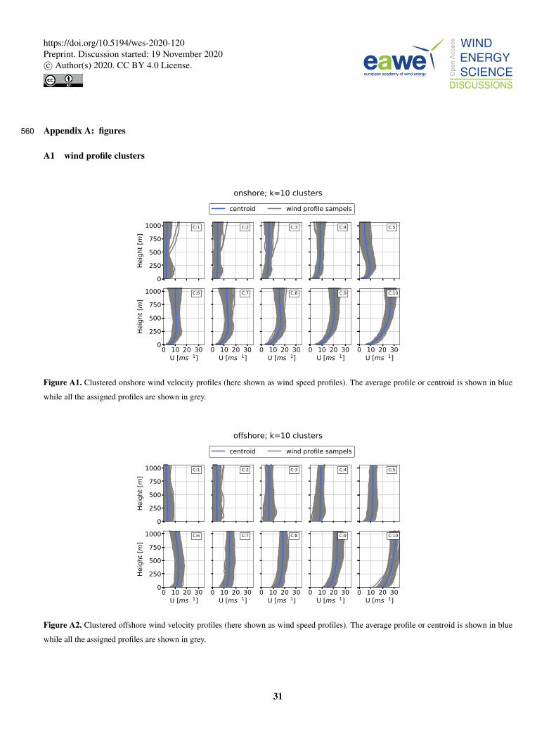
Appendix A: figures560

A1 wind profile clusters

0250500750

1000

Height [m

]

C:1 C:2 C:3

centroid wind rofile sam els

C:4 C:5

0 10 20 30U [ms−1]

0250500750

1000

Height [m

]

C:6

0 10 20 30U [ms−1]

C:7

0 10 20 30U [ms−1]

C:8

0 10 20 30U [ms−1]

C:9

0 10 20 30U [ms−1]

C:10

onshore; k=10 clusters

Figure A1. Clustered onshore wind velocity profiles (here shown as wind speed profiles). The average profile or centroid is shown in blue

while all the assigned profiles are shown in grey.

0250500750

1000

Height [m

]

C:1 C:2 C:3

centroid wind rofile sam els

C:4 C:5

0 10 20 30U [ms−1]

0250500750

1000

Height [m

]

C:6

0 10 20 30U [ms−1]

C:7

0 10 20 30U [ms−1]

C:8

0 10 20 30U [ms−1]

C:9

0 10 20 30U [ms−1]

C:10

offshore; k=10 clusters

Figure A2. Clustered offshore wind velocity profiles (here shown as wind speed profiles). The average profile or centroid is shown in blue

while all the assigned profiles are shown in grey.

31


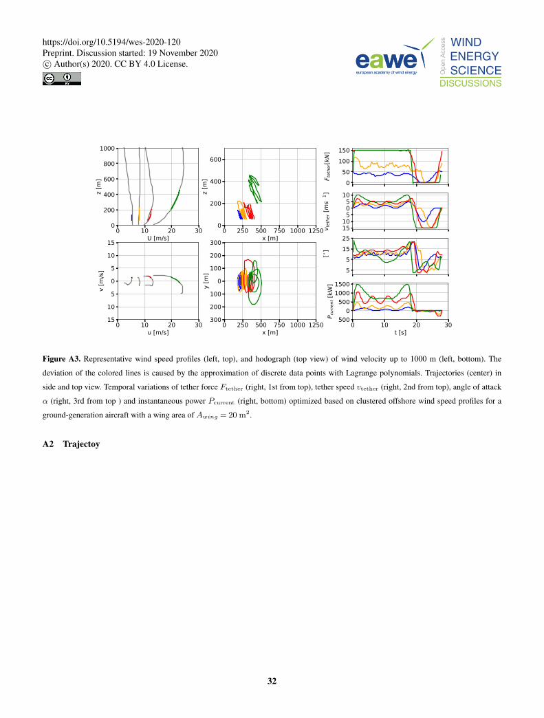
0 10 20 30U [m/s]

0

200

400

600

800

1000

z [m]

0 250 500 750 1000 1250x [m]

0

200

400

600

z [m]

0 250 500 750 1000 1250x [m]

−300

−200

−100

0

100

200

300

y [m

]

050

100150

F tethe

r[kN]

−15−10−505

10

v tethe

r [ms−

1 ]

−55

1525

α [∘]

0 10 20 30t [s]

−5000

50010001500

P current [k

∘]

0 10 20 30u [m/s]

−15

−10

−5

0

5

10

15

v [m

/s]

Figure A3. Representative wind speed profiles (left, top), and hodograph (top view) of wind velocity up to 1000 m (left, bottom). The

deviation of the colored lines is caused by the approximation of discrete data points with Lagrange polynomials. Trajectories (center) in

side and top view. Temporal variations of tether force Ftether (right, 1st from top), tether speed vtether (right, 2nd from top), angle of attack

α (right, 3rd from top ) and instantaneous power Pcurrent (right, bottom) optimized based on clustered offshore wind speed profiles for a

ground-generation aircraft with a wing area of Awing = 20 m2.

A2 Trajectoy

32


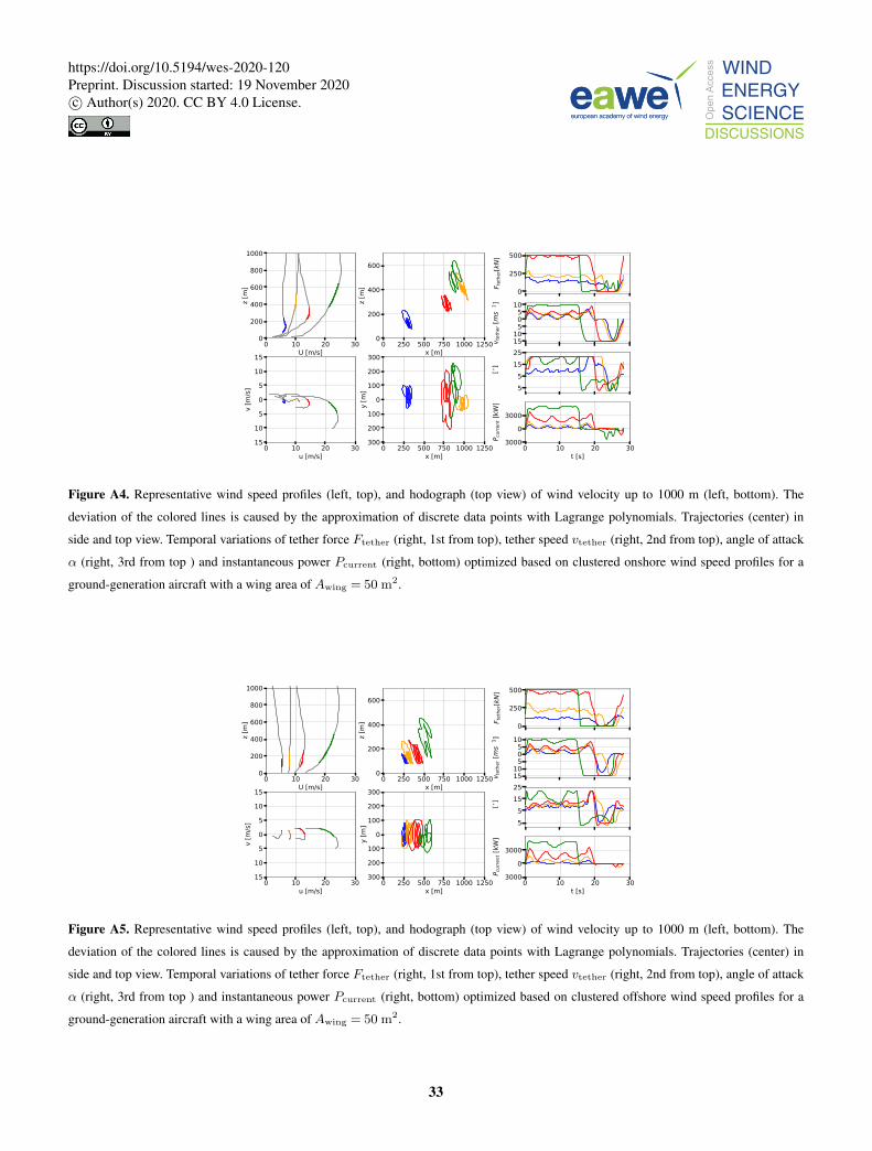
0 10 20 30U [m/s]

0

200

400

600

800

1000z [

m]

0 250 500 750 1000 1250x [m]

0

200

400

600

z [m]

0 250 500 750 1000 1250x [m]

−300

−200

−100

0

100

200

300y [m

]

0

250

500

F tethe

r[kN]

−15−10−505

10

v tethe

r [ms−

1 ]

−55

1525

α [∘]

0 10 20 30t [s]

−30000

3000

P current [k

∘]

0 10 20 30u [m/s]

−15

−10

−5

0

5

10

15

v [m

/s]




α (right, 3rd from top ) and instantaneous power Pcurrent (right, bottom) optimized based on clustered onshore wind speed profiles for a


0 10 20 30U [m/s]

0

200

400

600

800

1000

z [m]

0 250 500 750 1000 1250x [m]

0

200

400

600

z [m]

0 250 500 750 1000 1250x [m]

−300

−200

−100

0

100

200

300

y [m

]

0

250

500

F tethe

r[kN]

−15−10−505

10

v tethe

r [ms−

1 ]

−55

1525

α [∘]

0 10 20 30t [s]

−30000

3000

P current [k

∘]

0 10 20 30u [m/s]

−15

−10

−5

0

5

10

15

v [m

/s]




α (right, 3rd from top ) and instantaneous power Pcurrent (right, bottom) optimized based on clustered offshore wind speed profiles for a


33


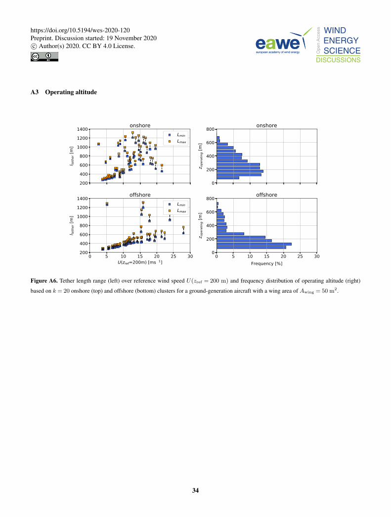
A3 Operating altitude

200400600800

100012001400

l tether [m

]

onshoreLmin

Lmax

0

200

400

600

800

z ope

ratin

g [m]

onshore

0 5 10 15 20 25 30U(zref=200m) [ms−1]

200400600800

100012001400

l tether [m

]

offshoreLmin

Lmax

0 5 10 15 20 25 30Frequency [%]

0

200

400

600

800z o

peratin

g [m]

offshore

Figure A6. Tether length range (left) over reference wind speed U(zref = 200 m) and frequency distribution of operating altitude (right)

based on k = 20 onshore (top) and offshore (bottom) clusters for a ground-generation aircraft with a wing area of Awing = 50 m2.

34


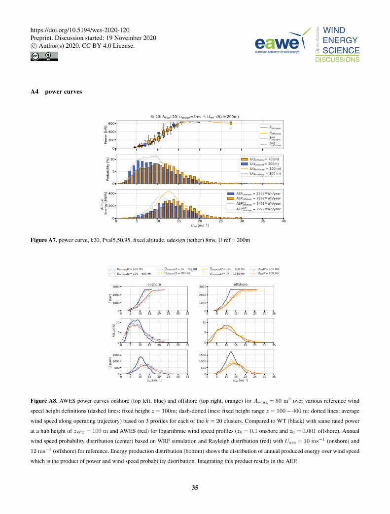
A4 power curves

0

200

400

600

Powe

r [kW

] PonshorePoffshorePWTonshore

PWToffshore

0

5

10

Prob

abilit

y [%

] U(zoffshore= 200m)U(zonshore= 200m)U(zoffshore = 100 m)U(zonshore = 100 m)

0 5 10 15 20 25 30 35 40Uref [ms−1]

0

200

400

Annu

a

Ene

rg)

[MW

h] AEPonshore = 2333MWh/)earAEPoffshore = 2892MWh/)earAEPWT

offshore = 3401MWh/)earAEPWT

onshore = 2292MWh/)ear

k: 20; Akite: 20; udesign=8ms−1; Uref :U(z= 200m)

Figure A7. power curve, k20, Pval5,50,95, fixed altitude, udesign (tether) 8ms, U ref = 200m

0 5 10 15 20 25 30 350

1000

2000

3000

P [kW]

onshore

Uonshore(z=100 m)Uonshore(z=100−400 m)

Uonshore(z=74−702 m)Uoffshore(z=100 m)

Uoffshore(z=100−400 m)Uoffshore(z=74−1265 m)

UWT(z=100 m)Ulog(z=100 m)

0 5 10 15 20 25 30 350

1000

2000

3000 offshore

0 5 10 15 20 25 30 350

5

10

f(Uref) [%

]

0 5 10 15 20 25 30 350

5

10

0 5 10 15 20 25 30 35Uref [ms−1]

0

500

1000

1500

E [kWh]

0 5 10 15 20 25 30 35Uref [ms−1]

0

500

1000

1500

Figure A8. AWES power curves onshore (top left, blue) and offshore (top right, orange) for Awing = 50 m2 over various reference wind

speed height definitions (dashed lines: fixed height z = 100m; dash-dotted lines: fixed height range z = 100− 400 m; dotted lines: average

wind speed along operating trajectory) based on 3 profiles for each of the k = 20 clusters. Compared to WT (black) with same rated power

at a hub height of zWT = 100 m and AWES (red) for logarithmic wind speed profiles (z0 = 0.1 onshore and z0 = 0.001 offshore). Annual

wind speed probability distribution (center) based on WRF simulation and Rayleigh distribution (red) with Uave = 10 ms−1 (onshore) and

12 ms−1 (offshore) for reference. Energy production distribution (bottom) shows the distribution of annual produced energy over wind speed

which is the product of power and wind speed probability distribution. Integrating this product results in the AEP.

35


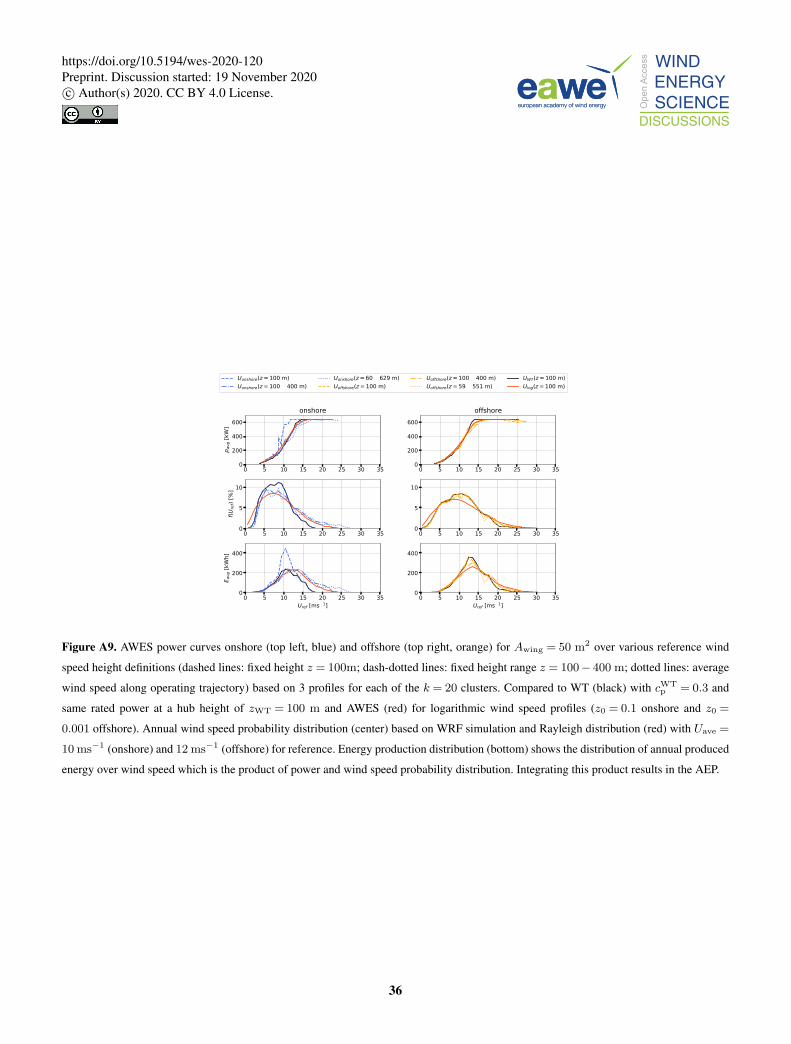
0 5 10 15 20 25 30 350

200

400

600

p avg [k

W]

onshore

Uonshore(z=100 m)Uonshore(z=100−400 m)

Uonshore(z=60−629 m)Uoffshore(z=100 m)

Uoffshore(z=100−400 m)Uoffshore(z=59−551 m)

UWT(z=100 m)Ulog(z=100 m)

0 5 10 15 20 25 30 350

200

400

600offshore

0 5 10 15 20 25 30 350

5

10

f(Uref) [%

]

0 5 10 15 20 25 30 350

5

10

0 5 10 15 20 25 30 35Uref [ms−1]

0

200

400

E avg [k

Wh]

0 5 10 15 20 25 30 35Uref [ms−1]

0

200

400

Figure A9. AWES power curves onshore (top left, blue) and offshore (top right, orange) for Awing = 50 m2 over various reference wind

speed height definitions (dashed lines: fixed height z = 100m; dash-dotted lines: fixed height range z = 100− 400 m; dotted lines: average

wind speed along operating trajectory) based on 3 profiles for each of the k = 20 clusters. Compared to WT (black) with cWTp = 0.3 and

same rated power at a hub height of zWT = 100 m and AWES (red) for logarithmic wind speed profiles (z0 = 0.1 onshore and z0 =

0.001 offshore). Annual wind speed probability distribution (center) based on WRF simulation and Rayleigh distribution (red) with Uave =

10 ms−1 (onshore) and 12 ms−1 (offshore) for reference. Energy production distribution (bottom) shows the distribution of annual produced

energy over wind speed which is the product of power and wind speed probability distribution. Integrating this product results in the AEP.

36


References565

Ampyx, .: Ampyx Power BV, https://www.ampyxpower.com/, last accessed: 2020-11-17.

Andersson, J., Åkesson, J., and Diehl, M.: CasADi: A Symbolic Package for Automatic Differentiation and Optimal Control, in: Recent

Advances in Algorithmic Differentiation, edited by Forth, S., Hovland, P., Phipps, E., Utke, J., and Walther, A., pp. 297–307, Springer

Berlin Heidelberg, Berlin, Heidelberg, 2012.

Archer, C. L., Colle, B. A., Veron, D. L., Veron, F., and Sienkiewicz, M. J.: On the predominance of unstable atmospheric conditions in570

the marine boundary layer offshore of the U.S. northeastern coast, Journal of Geophysical Research: Atmospheres, 121, 8869–8885,

https://doi.org/10.1002/2016JD024896, 2016.

Arya, P. and Holton, J.: Introduction to Micrometeorology, International Geophysics, Elsevier Science, 2001.

Aull, M., Stough, A., and Cohen, K.: Design Optimization and Sizing for Fly-Gen Airborne Wind Energy Systems, Automation, 1, 1–16,

2020.575

Banta, R. M.: Stable-boundary-layer regimes from the perspective of the low-level jet, Acta Geophysica, 56, 58–87,

https://doi.org/10.2478/s11600-007-0049-8, 2008.

Bronnenmeyer, T.: Optimal Control for Multi-Kite Emergency Trajectories, Master’s thesis, University of Stuttgart, https://cdn.syscop.de/

publications/Bronnenmeyer2018.pdf, last accessed: 2020-11-17, 2018.

Burton, T., ed.: Wind energy handbook, Wiley, Chichester, West Sussex, 2nd ed edn., https://doi.org/10.1002/9781119992714, 2011.580

Champion, K. S. W., Cole, A. E., and Kantor, A. J.: Chapter 14 Standard and Reference Atmospheres, 1985.

Cherubini, A., Papini, A., Vertechy, R., and Fontana, M.: Airborne Wind Energy Systems: A review of the technologies, Renewable and

Sustainable Energy Reviews, 51, 1461–1476, https://doi.org/10.1016/j.rser.2015.07.053, 2015.

De Schutter, J., Leuthold, R., and Diehl, M.: Optimal Control of a Rigid-Wing Rotary Kite System for Airborne Wind Energy, in: Proceedings

of the European Control Conference (ECC), 2018.585

De Schutter, J., Leuthold, R., Bronnenmeyer, T., Paelinck, R., and Diehl, M.: Optimal control of stacked multi-kite systems for utility-scale

airborne wind energy, in: 2019 IEEE 58th Conference on Decision and Control (CDC), pp. 4865–4870, 2019.

Dee, D. P., Uppala, S. M., Simmons, A. J., Berrisford, P., Poli, P., Kobayashi, S., Andrae, U., Balmaseda, M. A., Balsamo, G., Bauer,

P., Bechtold, P., Beljaars, A. C. M., van de Berg, L., Bidlot, J., Bormann, N., Delsol, C., Dragani, R., Fuentes, M., Geer, A. J., Haim-

berger, L., Healy, S. B., Hersbach, H., Hólm, E. V., Isaksen, L., Kållberg, P., Köhler, M., Matricardi, M., McNally, A. P., Monge-Sanz,590

B. M., Morcrette, J.-J., Park, B.-K., Peubey, C., de Rosnay, P., Tavolato, C., Thépaut, J.-N., and Vitart, F.: The ERA-Interim reanalysis:

configuration and performance of the data assimilation system, Quarterly Journal of the Royal Meteorological Society, 137, 553–597,

https://doi.org/10.1002/qj.828, 2011.

Donlon, C. J., Martin, M., Stark, J., Roberts-Jones, J., Fiedler, E., and Wimmer, W.: The Operational Sea Surface Temperature and Sea Ice

Analysis (OSTIA) system, Remote Sensing of Environment, 116, 140–158, https://doi.org/10.1016/j.rse.2010.10.017, 2012.595

Dörenkämper, M., Optis, M., Monahan, A., and Steinfeld, G.: On the Offshore advection of Boundary-Layer Structures and the Influence on

Offshore Wind Conditions, Boundary-Layer Meteorol., 155, 459–482, https://doi.org/10.1007/s10546-015-0008-x, 2015.

Dörenkämper, M., Stoevesandt, B., and Heinemann, D.: Derivation of an offshore wind index for the German bight from high-resolution

mesoscale simulation data, Proceedings of DEWEK - German Offshore Wind Energy Conference, p. 5, 2017.

Dörenkämper, M., Olsen, B. T., Witha, B., Hahmann, A. N., Davis, N. N., Barcons, J., Ezber, Y., García-Bustamante, E., González-Rouco,600

J. F., Navarro, J., Sastre-Marugán, M., Sı̄le, T., Trei, W., Žagar, M., Badger, J., Gottschall, J., Sanz Rodrigo, J., and Mann, J.: The

37


Making of the New European Wind Atlas – Part 2: Production and evaluation, Geoscientific Model Development, 13, 5079–5102,

https://doi.org/10.5194/gmd-13-5079-2020, 2020.

Emeis, S.: Wind energy meteorology: atmospheric physics for wind power generation, Springer, Heidelberg, 2018.

Fagiano, L. and Milanese, M.: Airborne Wind Energy: An overview, in: 2012 American Control Conference (ACC), pp. 3132–3143, IEEE,605

https://doi.org/10.1109/ACC.2012.6314801, 2012.

Floors, R., Batchvarova, E., Gryning, S.-E., Hahmann, A. N., Peña, A., and Mikkelsen, T.: Atmospheric boundary layer wind profile at

a flat coastal site - wind speed lidar measurements and mesoscale modeling results, Advances in Science and Research, 6, 155–159,

https://doi.org/10.5194/asr-6-155-2011, 2011.

Gaertner, E., Rinker, J., Sethuraman, L., Zahle, F., Anderson, B., Barter, G. E., Abbas, N. J., Meng, F., Bortolotti, P., Skrzypinski, W.,610

Scott, G. N., Feil, R., Bredmose, H., Dykes, K., Shields, M., Allen, C., and Viselli, A.: IEA Wind TCP Task 37: Definition of the IEA

15-Megawatt Offshore Reference Wind Turbine, https://doi.org/10.2172/1603478, 2020.

Gros, S., Zanon, M., and Diehl, M.: A relaxation strategy for the optimization of Airborne Wind Energy systems, in: 2013 European Control

Conference (ECC), pp. 1011–1016, https://doi.org/10.23919/ECC.2013.6669670, 2013.

Hahmann, A. N., Sı̄le, T., Witha, B., Davis, N. N., Dörenkämper, M., Ezber, Y., García-Bustamante, E., González-Rouco, J. F., Navarro,615

J., Olsen, B. T., and Söderberg, S.: The making of the New European Wind Atlas – Part 1: Model sensitivity, Geoscientific Model

Development, 13, 5053–5078, https://doi.org/10.5194/gmd-13-5053-2020, 2020.

Hersbach, H. and Dick, D.: ERA5 reanalysis is in production, http://www.ecmwf.int/en/newsletter/147/news/era5-reanalysis-production, last

accessed: 2019-10-22, 2016.

HSL: The HSL Mathematical Software Library, http://www.hsl.rl.ac.uk/, last accessed: 2020-06-14.620

International Electrotechnical Commission, ed.: Design requirements: amendment 1, no. 1,1 in Wind turbines, IEC, Geneva, ed. 3.0, 2010-10

edn., oCLC: 838280539, 2010.

Leuthold, R., De Schutter, J., Malz, E. C., Licitra, G., Gros, S., and Diehl, M.: Operational Regions of a Multi-Kite AWE System, in: 2018

European Control Conference (ECC), pp. 52–57, https://doi.org/10.23919/ECC.2018.8550199, 2018.

Licitra, G., Koenemann, J., Bürger, A., Williams, P., Ruiterkamp, R., and Diehl, M.: Performance assessment of a rigid wing Airborne Wind625

Energy pumping system, Energy, 173, 569–585, https://doi.org/10.1016/j.energy.2019.02.064, 2019.

Loyd, M. L.: Crosswind kite power (for large-scale wind power production), Journal of Energy, 4, 106–111, https://doi.org/10.2514/3.48021,

1980.

Lunney, E., Ban, M., Duic, N., and Foley, A.: A state-of-the-art review and feasibility analysis of high altitude wind power in Northern

Ireland, Renewable and Sustainable Energy Reviews, 68, 899 – 911, https://doi.org/10.1016/j.rser.2016.08.014, 2017.630

Malz, E., Koenemann, J., Sieberling, S., and Gros, S.: A reference model for airborne wind energy systems for optimization and control,

Renewable Energy, 140, 1004 – 1011, https://doi.org/10.1016/j.renene.2019.03.111, 2019.

Malz, E., Hedenus, F., Göransson, L., Verendel, V., and Gros, S.: Drag-mode airborne wind energy vs. wind turbines: An analysis of power

production, variability and geography, Energy, 193, 116 765, https://doi.org/10.1016/j.energy.2019.116765, 2020.

Molina-García, A., Fernández-Guillamón, A., Gómez-Lázaro, E., Honrubia-Escribano, A., and Bueso, M. C.: Vertical Wind Pro-635

file Characterization and Identification of Patterns Based on a Shape Clustering Algorithm, IEEE Access, 7, 30 890–30 904,

https://doi.org/10.1109/ACCESS.2019.2902242, 2019.

Nakanishi, M. and Niino, H.: Development of an Improved Turbulence Closure Model for the Atmospheric Boundary Layer, Journal of the

Meteorological Society of Japan, 87, 895–912, https://doi.org/10.2151/jmsj.87.895, 2009.

38


Obukhov, A. M.: Turbulence in an atmosphere with a non-uniform temperature, Boundary-Layer Meteorology, 2, 7–29,640

https://doi.org/10.1007/BF00718085, 1971.

Olauson, J.: ERA5: The new champion of wind power modelling?, Renewable Energy, 126, 322–331,

https://doi.org/10.1016/j.renene.2018.03.056, 2018.

Optis, M., Monahan, A., and Bosveld, F. C.: Limitations and breakdown of Monin–Obukhov similarity theory for wind profile extrapolation

under stable stratification, Wind Energy, 19, 1053–1072, https://doi.org/10.1002/we.1883, 2016.645

Peña, A., Gryning, S.-E., and Floors, R.: Lidar observations of marine boundary-layer winds and heights: a preliminary study, Meteorologis-

che Zeitschrift, 24, 581–589, https://doi.org/10.1127/metz/2015/0636, 2015.

Pedregosa, F., Varoquaux, G., Gramfort, A., Michel, V., Thirion, B., Grisel, O., Blondel, M., Prettenhofer, P., Weiss, R., Dubourg, V.,

Vanderplas, J., Passos, A., Cournapeau, D., Brucher, M., Perrot, M., and Duchesnay, E.: Scikit-learn: Machine Learning in Python, Journal

of Machine Learning Research, 12, 2825–2830, 2011.650

Salvação, N. and Guedes Soares, C.: Wind resource assessment offshore the Atlantic Iberian coast with the WRF model, Energy, 145, 276 –

287, https://doi.org/10.1016/j.energy.2017.12.101, 2018.

Schelbergen, M., Kalverla, P. C., Schmehl, R., and Watson, S. J.: Clustering wind profile shapes to estimate airborne wind energy production,

Wind Energy Science, 5, 1097–1120, https://doi.org/10.5194/wes-5-1097-2020, 2020.

Sempreviva, A. M. and Gryning, S.-E.: Humidity fluctuations in the marine boundary layer measured at a coastal site with an infrared655

humidity sensor, Boundary-Layer Meteorology, 77, 331–352, https://doi.org/10.1007/BF00123531, 1996.

Skamarock, W., Klemp, J., Dudhia, J., Gill, D., Barker, D., Duda, M., Huang, X., Wang, W., and Powers, J.: A description of the advanced

research WRF version 3, Tech. Rep. NCAR/TN–475+STR, NCAR - National Center for Atmospheric Research, Boulder, Colorado, USA,

http://n2t.net/ark:/85065/d72n51q1, last accessed: 2020-11-17, 2008.

Sommerfeld, M., Crawford, C., Monahan, A., and Bastigkeit, I.: LiDAR-based characterization of mid-altitude wind conditions for airborne660

wind energy systems, Wind Energy, 22, 1101–1120, https://doi.org/10.1002/we.2343, 2019a.

Sommerfeld, M., Dörenkämper, M., Steinfeld, G., and Crawford, C.: Improving mesoscale wind speed forecasts using lidar-based observation

nudging for airborne wind energy systems, Wind Energy Science, 4, 563–580, https://doi.org/10.5194/wes-4-563-2019, 2019b.

Sommerfeld, M., Dörenkämper, M., Steinfeld, G., and Crawford, C.: Improving mesoscale wind speed forecasts using lidar-based observation

nudging for airborne wind energy systems, Wind Energy Science, 4, 563–580, https://doi.org/10.5194/wes-4-563-2019, 2019c.665

Stull, R. B.: An Introduction to Boundary Layer Meteorology, vol. 13, Springer Science & Business Media, https://doi.org/10.1007/978-94-

009-3027-8, 2012.

Wächter, A. and Biegler, L. T.: On the implementation of an interior-point filter line-search algorithm for large-scale nonlinear programming,

Mathematical Programming, 106, 25–57, https://doi.org/10.1007/s10107-004-0559-y, 2006.

39


Documents

Offshore and onshore ground-generation airborne wind ... - WES