Embed Size (px)
Citation preview
Omega risk model with tax
Zhenyu Cui ∗
Draft: March 29, 2014
Abstract
In this paper we study the Omega risk model with surplus-dependent tax pay-ments in a time-homogeneous diffusion setting. The new model incorporates practi-cal features from both the Omega risk model(Albrecher and Gerber and Shiu (2011))and the risk model with tax(Albrecher and Hipp (2007)). We explicitly characterizethe Laplace transform of the occupation time of an Azema-Yor process(e.g. a processrefracted by functionals of its running maximum) below a constant level until thefirst hitting time of another Azema-Yor process or until an independent exponentialtime. This result unifies and extends recent literature(Li and Zhou (2013) and Zhang(2014)) incorporating some of their results as special cases. We explicitly character-ize the Laplace transform of the time of bankruptcy in the Omega risk model withtax and discuss an extension to integral functionals. Finally we present examplesusing a Brownian motion with drift.
Math Subject Classification 60G44 91B25 91B70Key-words: Time-homogeneous diffusion; Azema-Yor process; occupation time; Laplacetransform; risk model with tax; Omega risk model.
∗Corresponding Author. Zhenyu Cui is with the department of Mathematics at Brooklyn College ofthe City University of New York, Ingersoll Hall, 2900 Bedford Ave, Brooklyn, NY11210, United States.Tel.: +1718-951-5600, ext. 6892 Fax: +1718-951-4674. Email: [email protected]
1
1 Introduction
The Omega risk model was first introduced by Albrecher, Gerber and Shiu (2011), andit distinguishes the ruin time(negative surplus) from the time of bankruptcy of a com-pany(occupation time of the negative surplus exceeds a grace period).
The risk model with tax was first introduced in Albrecher and Hipp (2007), wherea constant tax rate is applied to the compound Poisson risk model at profitable times.In a time-homogeneous diffusion setting, Li, Tang and Zhou (2013) introduce a diffusionrisk model with tax and model the ruin time of the company by its two-sided exit time.In the Levy insurance model with tax, Kyprianou and Zhou (2009) obtain explicitly thetwo-sided exit time, the expected present value of tax until ruin, and the generalizedGerber-Shiu function. Renaud (2009) obtains explicit expressions of the distribution ofthe tax payments made over the lifetime of the company.
We make three contributions to the current literature. First, we obtain the Laplacetransform of the occupation time of an Azema-Yor process below a constant level until thefirst hitting time of another Azema-Yor process or until an independent exponential time.This result unifies and extends recent literature(Li, Tang and Zhou (2013), Li and Zhou(2013) and Zhang (2014)) incorporating some of their results as special cases. Second,we propose the “Omega risk model with tax” to model the ruin and bankruptcy of aninsurance company. This allows a more practical view in the modeling of bankruptcy,because an insurance company under distress is subject to tax, which may further weakentheir solvency, and the company is considered bankrupt only when its surplus value is belowa critical level beyond a“grace period”. We explicitly characterize the Laplace transform ofthe time of bankruptcy. Third, as an application of the main results, we obtain the Laplacetransforms of the occupation times related to both the (absolute) drawdown and therelative drawdown until respectively the first hitting time or an independent exponentialtime. We also discuss an extension to integral functionals through stochastic time change.
The paper is organized as follows: Section 2 reviews the preliminary results on theOmega risk model and the risk model with tax. Section 3 gives the main results, namelythe explicit Laplace transforms of the occupation time of an Azema-Yor process belowa constant level until the first hitting time of another Azema-Yor process or until anindependent exponential time. As an application, we propose the “Omega risk modelwith tax”, and determine the Laplace transform of the time of bankruptcy. We alsodiscuss other interesting applications involving both the absolute and relative drawdownprocesses of the before-tax and after-tax processes, and the extension to a more generalbankruptcy function. Section 4 provides examples using a standard Brownian motion withdrift. Section 5 concludes the paper with future research directions.
2 Preliminaries
Recently, there are two strands of literature with one looking at a new definition of “ruin”,and the other considering a diffusion risk model refracted by its running maximum named
2
the “risk model with tax”. We review relevant literature here and in Section 3 we willcombine them to propose and study the “Omega risk model with tax”.
2.1 The Omega risk model
Classical ruin theory assumes that ruin or bankruptcy will occur at the first time whenthe surplus value of an insurance company is negative. For a pointer to the literature inthis area, please refer to Gerber and Shiu (1998). Recently, the “Omega risk model” hasbeen proposed and studied in a series of papers starting with Albrecher, Gerber and Shiu(2011). This model distinguishes between ruin (negative surplus value) and bankruptcy(going out of business). The company continues operation even with a period of negativesurplus value, and is declared bankrupt if this period exceeds a threshold “grace period”.They introduce a bankruptcy rate function ω(x), where x < 0 denotes the value of negativesurplus value, and it represents the probability of bankruptcy within dt time units. TheOmega risk model is based on the study of the occupation time of the risk process belowa constant level. The occupation time of of a spectrally negative Levy process has beenstudied in Landriault, Renaud and Zhou ((2011) (2014)) and Loeffen, Renaud and Zhou(2014). The occupation time of a refracted Levy process(Kyprianou and Loeffen (2010))has been studied in Renaud (2014). This paper focuses on the diffusion risk model similaras in Li and Zhou (2013).
Given a complete filtered probability space (Ω,F ,Ft, P ) with state space J = (l,∞),−∞ 6l <∞, consider a J-valued regular time-homogeneous diffusion X = (Xt)t∈[0,∞) which sat-isfies the stochastic differential equation(SDE)
dXt = µ(Xt) dt + σ(Xt) dWt, X0 = x ∈ J, (1)
where W is a Ft-Brownian motion and µ(·) and σ(·) > 0 are Borel functions satisfying thefollowing conditions: there exists a constant C > 0 such that, for all x1, x2 ∈ J
| µ(x1)− µ(x2) | + | σ(x1)− σ(x2) | 6 C | x1 − x2 |, µ2(x1) + σ2(x1) 6 C2(1 + x21),(2)
Condition (2) guarantees that the SDE (1) has a unique solution that possesses the strongMarkov property (see p.40, p.107, Gihman and Skorohod (1972)).
In the following, we denote Px(·) , P (· | X0 = x) and Ex[·] , Ex[· | X0 = x]. Assumethat the before-tax value of the company is modeled by X with SDE (1). If we introducean auxiliary “bankruptcy monitoring” process N on the same probability space (with apossibly enlarged filtration to accommodate it), and assume that conditional on X, Nfollows a Poisson process with state-dependent intensity ω(Xt)1Xt<0, t > 0. Define thetime of bankruptcy τω as the first arrival time of the Poisson process N , i.e.
τω := inf
t > 0 :
∫ t
0
ω(Xs)1Xs<0ds > e1
, (3)
3
where e1 is an independent exponential random variable with unit rate. Similar as in Li andZhou (2013), for λ > 0, we can express the Laplace transform of the time of bankruptcyas
Ex[e−λτω ] = Px(τω < eλ) = 1− Ex
[e−
∫ eλ0 ω(Xs)1Xs<0ds
]. (4)
2.2 Risk model with surplus-dependent tax
The risk model with tax was introduced by Albrecher and Hipp (2007) in the case of aconstant tax rate, and was later extended by Albrecher, Renaud and Zhou (2008) andKyprianou and Zhou (2009) to the case where there is a non-negative state-dependenttax payment paid immediately when the surplus value of the company is at a runningmaximum.
Assume that the before-tax value of the company is modeled by the diffusion X in(1). Introduce a state-dependent tax: whenever the process Xt coincides with its runningmaximum X t, the firm pays tax at rate γ(X t), where γ(·) : [x,∞) → [0, 1) is a Borelmeasurable function. The value process after taxation is denoted as (Ut)t>0, and satisfies
dUt = dXt − γ(X t)dX t, U0 = X0 = x, t > 0, (5)
Kyprianou and Zhou (2009) introduce the following function
γ(u) = u−∫ u
x
γ(z)dz = x+
∫ u
x
(1− γ(z))dz, u > x. (6)
Notice that x < γ(u) 6 u. We have the following representation Ut = Xt −X t + γ(X t).
3 Omega risk model with surplus-dependent tax
We combine the practical features of the “Omega risk model” and the “risk model withtax” to propose the “Omega risk model with tax”, where we use (5) to model the after-tax surplus value of an insurance company. Li, Tang and Zhou (2013) define the time ofdefault with tax as the two-sided exit time of U from the constant boundaries. We definethe time of bankruptcy of the company as the first time the occupation time exceeds anindependent exponential time with unit rate.
Ut is a special case of the so called Azema-Yor process introduced in Azema and Yor(1979), which is a process refracted by functionals of its running maximum (see also theterminology in Albrecher and Ivanovs (2014)). We first obtain general Laplace transformsof the occupation time of an Azema-Yor process below a constant level until the firsthitting time of another Azema-Yor process or until an independent exponential time. Tothe best of our knowledge, these results are new and are of independent interest. As anapplication, we obtain the explicit Laplace transform of the “time of bankruptcy” of the“Omega risk model with tax”. Our general formula contains some results in Li and Zhou(2013) and Zhang (2014) as special cases.
4
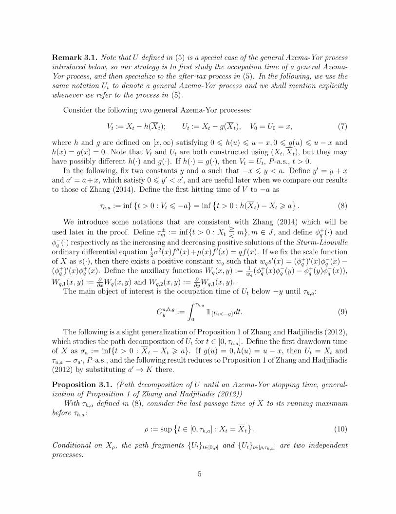
Remark 3.1. Note that U defined in (5) is a special case of the general Azema-Yor processintroduced below, so our strategy is to first study the occupation time of a general Azema-Yor process, and then specialize to the after-tax process in (5). In the following, we use thesame notation Ut to denote a general Azema-Yor process and we shall mention explicitlywhenever we refer to the process in (5).
Consider the following two general Azema-Yor processes:
Vt := Xt − h(X t); Ut := Xt − g(X t), V0 = U0 = x, (7)
where h and g are defined on [x,∞) satisfying 0 6 h(u) 6 u − x, 0 6 g(u) 6 u − x andh(x) = g(x) = 0. Note that Vt and Ut are both constructed using (Xt, X t), but they mayhave possibly different h(·) and g(·). If h(·) = g(·), then Vt = Ut, P -a.s., t > 0.
In the following, fix two constants y and a such that −x 6 y < a. Define y′ = y + xand a′ = a+x, which satisfy 0 6 y′ < a′, and are useful later when we compare our resultsto those of Zhang (2014). Define the first hitting time of V to −a as
τh,a := inf t > 0 : Vt 6 −a = inft > 0 : h(X t)−Xt > a
. (8)
We introduce some notations that are consistent with Zhang (2014) which will be
used later in the proof. Define τ±m := inft > 0 : Xt T m,m ∈ J , and define φ+q (·) and
φ−q (·) respectively as the increasing and decreasing positive solutions of the Sturm-Liouvilleordinary differential equation 1
2σ2(x)f ′′(x)+µ(x)f ′(x) = qf(x). If we fix the scale function
of X as s(·), then there exists a positive constant wq such that wqs′(x) = (φ+
q )′(x)φ−q (x)−(φ+
q )′(x)φ+q (x). Define the auxiliary functions Wq(x, y) := 1
wq(φ+
q (x)φ−q (y)− φ+q (y)φ−q (x)),
Wq,1(x, y) := ∂∂xWq(x, y) and Wq,2(x, y) := ∂
∂yWq,1(x, y).
The main object of interest is the occupation time of Ut below −y until τh,a:
Ga,h,gy :=
∫ τh,a
0
1Ut<−ydt. (9)
The following is a slight generalization of Proposition 1 of Zhang and Hadjiliadis (2012),which studies the path decomposition of Ut for t ∈ [0, τh,a]. Define the first drawdown timeof X as σa := inft > 0 : X t − Xt > a. If g(u) = 0, h(u) = u − x, then Ut = Xt andτu,a = σa′ , P -a.s., and the following result reduces to Proposition 1 of Zhang and Hadjiliadis(2012) by substituting a′ → K there.
Proposition 3.1. (Path decomposition of U until an Azema-Yor stopping time, general-ization of Proposition 1 of Zhang and Hadjiliadis (2012))
With τh,a defined in (8), consider the last passage time of X to its running maximumbefore τh,a:
ρ := supt ∈ [0, τh,a] : Xt = X t
. (10)
Conditional on Xρ, the path fragments Utt∈[0,ρ] and Utt∈[ρ,τh,a] are two independentprocesses.
5
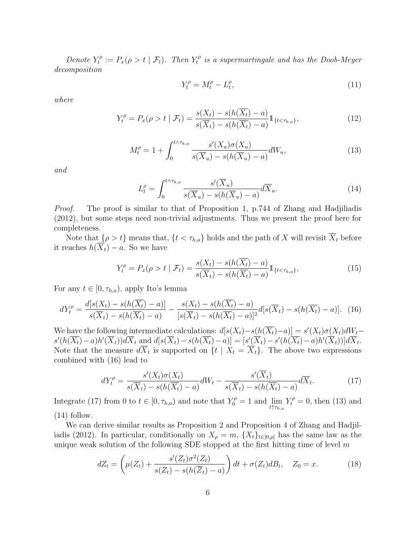
Denote Y ρt := Px(ρ > t | Ft). Then Y ρ
t is a supermartingale and has the Doob-Meyerdecomposition
Y ρt = Mρ
t − Lρt , (11)
where
Y ρt = Px(ρ > t | Ft) =
s(Xt)− s(h(Xt)− a)
s(X t)− s(h(Xt)− a)1t<τh,a, (12)
Mρt = 1 +
∫ t∧τh,a
0
s′(Xu)σ(Xu)
s(Xu)− s(h(Xu)− a)dWu, (13)
and
Lρt =
∫ t∧τh,a
0
s′(Xu)
s(Xu)− s(h(Xu)− a)dXu. (14)
Proof. The proof is similar to that of Proposition 1, p.744 of Zhang and Hadjiliadis(2012), but some steps need non-trivial adjustments. Thus we present the proof here forcompleteness.
Note that ρ > t means that, t < τh,a holds and the path of X will revisit X t beforeit reaches h(X t)− a. So we have
Y ρt = Px(ρ > t | Ft) =
s(Xt)− s(h(Xt)− a)
s(X t)− s(h(Xt)− a)1t<τh,a, (15)
For any t ∈ [0, τh,a), apply Ito’s lemma
dY ρt =
d[s(Xt)− s(h(Xt)− a)]
s(X t)− s(h(Xt)− a)− s(Xt)− s(h(Xt)− a)
[s(X t)− s(h(Xt)− a)]2d[s(X t)− s(h(Xt)− a)]. (16)
We have the following intermediate calculations: d[s(Xt)−s(h(Xt)−a)] = s′(Xt)σ(Xt)dWt−s′(h(Xt)−a)h′(X t))dX t and d[s(X t)−s(h(Xt)−a)] = [s′(X t)−s′(h(Xt)−a)h′(X t))]dX t.Note that the measure dX t is supported on t | Xt = X t. The above two expressionscombined with (16) lead to
dY ρt =
s′(Xt)σ(Xt)
s(X t)− s(h(Xt)− a)dWt −
s′(X t)
s(X t)− s(h(Xt)− a)dX t. (17)
Integrate (17) from 0 to t ∈ [0, τh,a) and note that Y ρ0 = 1 and lim
t↑τh,aY ρt = 0, then (13) and
(14) follow.We can derive similar results as Proposition 2 and Proposition 4 of Zhang and Hadjil-
iadis (2012). In particular, conditionally on Xρ = m, Xtt∈[0,ρ] has the same law as theunique weak solution of the following SDE stopped at the first hitting time of level m
dZt =
(µ(Zt) +
s′(Zt)σ2(Zt)
s(Zt)− s(h(Zt)− a)
)dt+ σ(Zt)dBt, Z0 = x. (18)
6
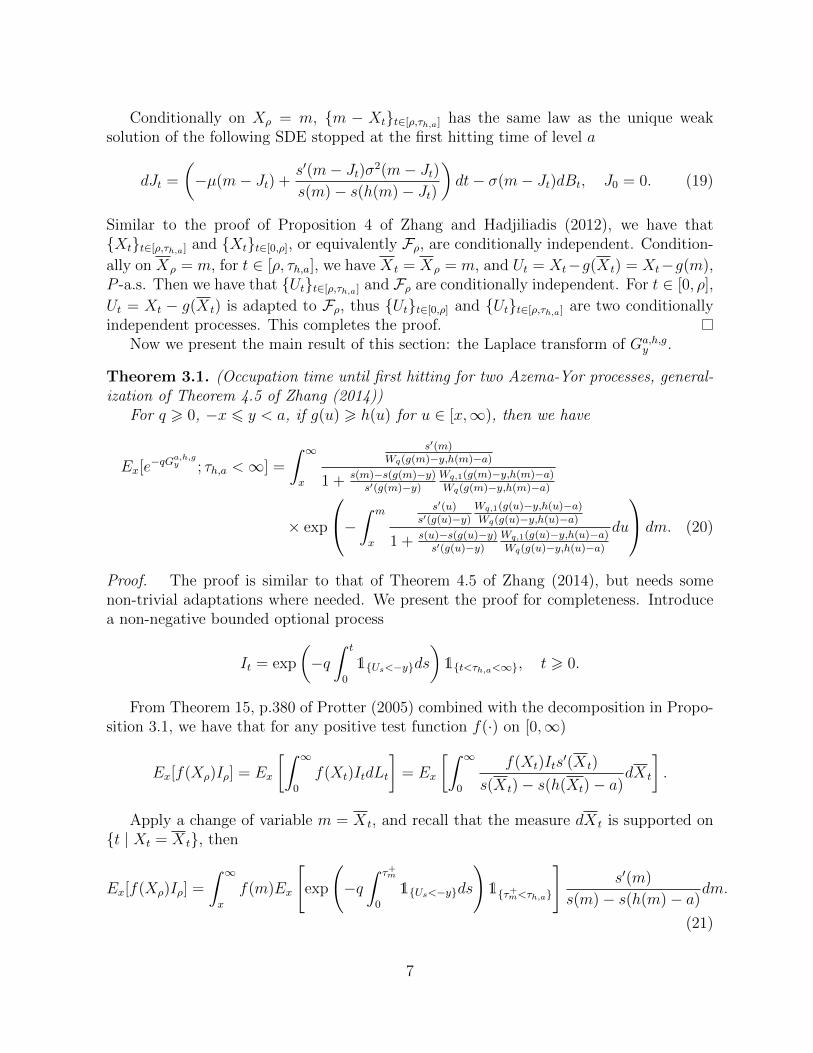
Conditionally on Xρ = m, m − Xtt∈[ρ,τh,a] has the same law as the unique weaksolution of the following SDE stopped at the first hitting time of level a
dJt =
(−µ(m− Jt) +
s′(m− Jt)σ2(m− Jt)s(m)− s(h(m)− Jt)
)dt− σ(m− Jt)dBt, J0 = 0. (19)
Similar to the proof of Proposition 4 of Zhang and Hadjiliadis (2012), we have thatXtt∈[ρ,τh,a] and Xtt∈[0,ρ], or equivalently Fρ, are conditionally independent. Condition-
ally on Xρ = m, for t ∈ [ρ, τh,a], we have X t = Xρ = m, and Ut = Xt−g(X t) = Xt−g(m),P -a.s. Then we have that Utt∈[ρ,τh,a] and Fρ are conditionally independent. For t ∈ [0, ρ],
Ut = Xt − g(X t) is adapted to Fρ, thus Utt∈[0,ρ] and Utt∈[ρ,τh,a] are two conditionallyindependent processes. This completes the proof.
Now we present the main result of this section: the Laplace transform of Ga,h,gy .
Theorem 3.1. (Occupation time until first hitting for two Azema-Yor processes, general-ization of Theorem 4.5 of Zhang (2014))
For q > 0, −x 6 y < a, if g(u) > h(u) for u ∈ [x,∞), then we have
Ex[e−qGa,h,gy ; τh,a <∞] =
∫ ∞x
s′(m)Wq(g(m)−y,h(m)−a)
1 + s(m)−s(g(m)−y)s′(g(m)−y)
Wq,1(g(m)−y,h(m)−a)Wq(g(m)−y,h(m)−a)
× exp
−∫ m
x
s′(u)s′(g(u)−y)
Wq,1(g(u)−y,h(u)−a)Wq(g(u)−y,h(u)−a)
1 + s(u)−s(g(u)−y)s′(g(u)−y)
Wq,1(g(u)−y,h(u)−a)Wq(g(u)−y,h(u)−a)
du
dm. (20)
Proof. The proof is similar to that of Theorem 4.5 of Zhang (2014), but needs somenon-trivial adaptations where needed. We present the proof for completeness. Introducea non-negative bounded optional process
It = exp
(−q∫ t
0
1Us<−yds
)1t<τh,a<∞, t > 0.
From Theorem 15, p.380 of Protter (2005) combined with the decomposition in Propo-sition 3.1, we have that for any positive test function f(·) on [0,∞)
Ex[f(Xρ)Iρ] = Ex
[∫ ∞0
f(Xt)ItdLt
]= Ex
[∫ ∞0
f(Xt)Its′(X t)
s(X t)− s(h(Xt)− a)dX t
].
Apply a change of variable m = X t, and recall that the measure dX t is supported ont | Xt = X t, then
Ex[f(Xρ)Iρ] =
∫ ∞x
f(m)Ex
[exp
(−q∫ τ+m
0
1Us<−yds
)1τ+m<τh,a
]s′(m)
s(m)− s(h(m)− a)dm.
(21)
7
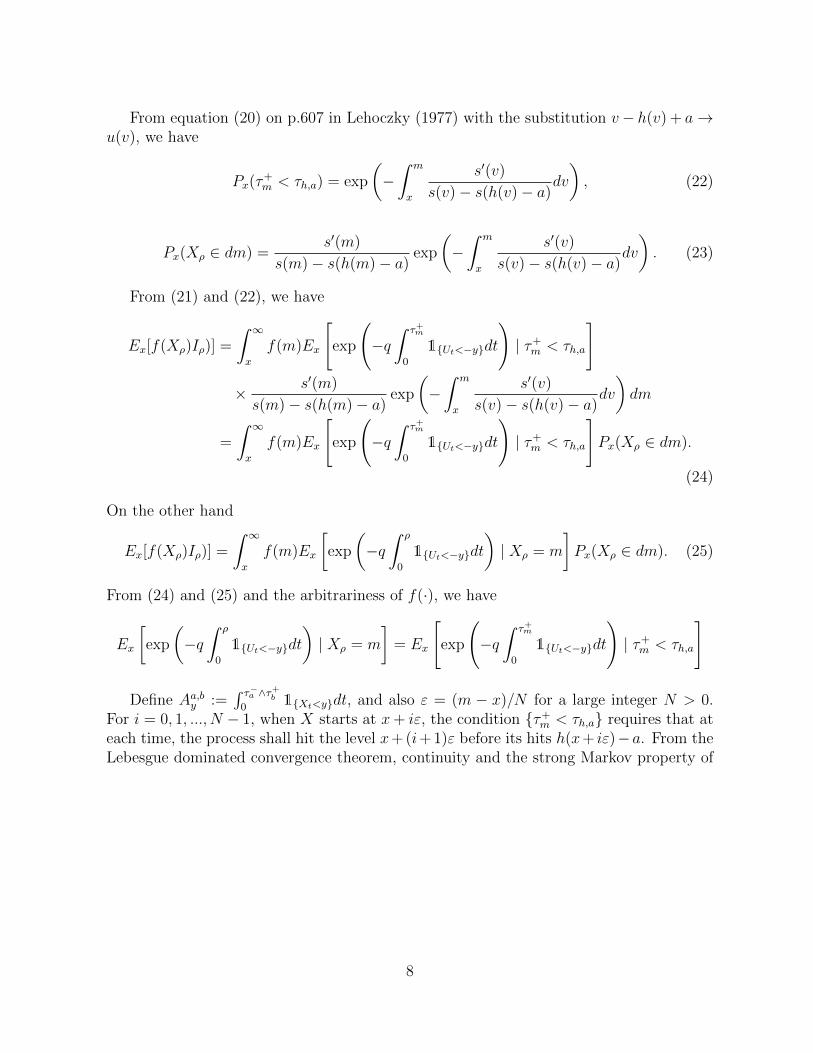
From equation (20) on p.607 in Lehoczky (1977) with the substitution v− h(v) + a→u(v), we have
Px(τ+m < τh,a) = exp
(−∫ m
x
s′(v)
s(v)− s(h(v)− a)dv
), (22)
Px(Xρ ∈ dm) =s′(m)
s(m)− s(h(m)− a)exp
(−∫ m
x
s′(v)
s(v)− s(h(v)− a)dv
). (23)
From (21) and (22), we have
Ex[f(Xρ)Iρ)] =
∫ ∞x
f(m)Ex
[exp
(−q∫ τ+m
0
1Ut<−ydt
)| τ+m < τh,a
]
× s′(m)
s(m)− s(h(m)− a)exp
(−∫ m
x
s′(v)
s(v)− s(h(v)− a)dv
)dm
=
∫ ∞x
f(m)Ex
[exp
(−q∫ τ+m
0
1Ut<−ydt
)| τ+m < τh,a
]Px(Xρ ∈ dm).
(24)
On the other hand
Ex[f(Xρ)Iρ)] =
∫ ∞x
f(m)Ex
[exp
(−q∫ ρ
0
1Ut<−ydt
)| Xρ = m
]Px(Xρ ∈ dm). (25)
From (24) and (25) and the arbitrariness of f(·), we have
Ex
[exp
(−q∫ ρ
0
1Ut<−ydt
)| Xρ = m
]= Ex
[exp
(−q∫ τ+m
0
1Ut<−ydt
)| τ+m < τh,a
]
Define Aa,by :=∫ τ−a ∧τ+b0
1Xt<ydt, and also ε = (m − x)/N for a large integer N > 0.For i = 0, 1, ..., N − 1, when X starts at x+ iε, the condition τ+m < τh,a requires that ateach time, the process shall hit the level x+ (i+ 1)ε before its hits h(x+ iε)−a. From theLebesgue dominated convergence theorem, continuity and the strong Markov property of
8
X, we have
Ex
[exp
(−q∫ τ+m
0
1Ut<−ydt
)| τ+m < τh,a
]
= limN→∞
N−1∏i=0
Ex+iε
[e−qA
h(x+iε)−a,x+(i+1)εg(x+iε)−y | τ+x+(i+1)ε < τ+h(x+iε)−a
]= lim
N→∞exp
(log
(N−1∑i=0
Ex+iε
[e−qA
h(x+iε)−a,x+(i+1)εg(x+iε)−y | τ+x+(i+1)ε < τ+h(x+iε)−a
]))
= exp
(limN→∞
N−1∑i=0
(Ex+iε
[e−qA
h(x+iε)−a,x+(i+1)εg(x+iε)−y | τ+x+(i+1)ε < τ+h(x+iε)−a
]− 1))
= exp
∫ m
x
s′(u)
s(u)− s(h(u)− a)−
s′(u)s′(g(u)−y)
Wq,1(g(u)−y,h(u)−a)Wq(g(u)−y,h(u)−a)
1 + s(u)−s(g(u)−y)s′(g(u)−y)
Wq,1(g(u)−y,h(u)−a)Wq(g(u)−y,h(u)−a)
du , (26)
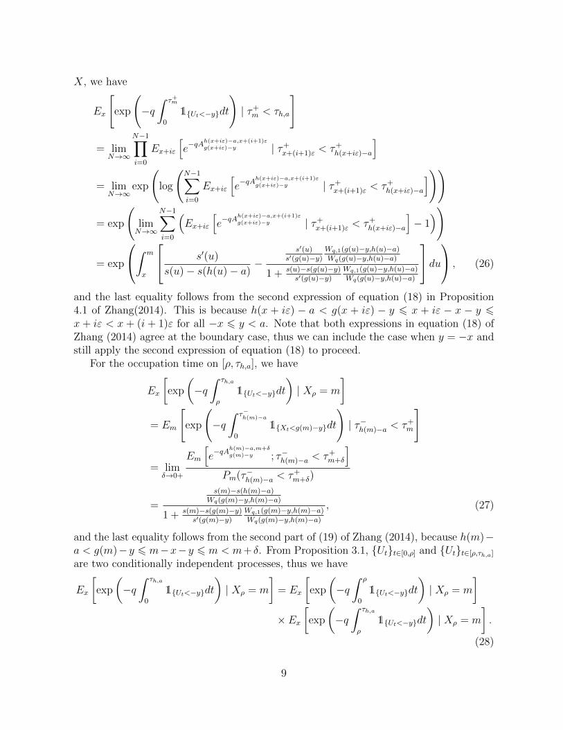
and the last equality follows from the second expression of equation (18) in Proposition4.1 of Zhang(2014). This is because h(x + iε) − a < g(x + iε) − y 6 x + iε − x − y 6x + iε < x + (i + 1)ε for all −x 6 y < a. Note that both expressions in equation (18) ofZhang (2014) agree at the boundary case, thus we can include the case when y = −x andstill apply the second expression of equation (18) to proceed.
For the occupation time on [ρ, τh,a], we have
Ex
[exp
(−q∫ τh,a
ρ
1Ut<−ydt
)| Xρ = m
]= Em
[exp
(−q∫ τ−
h(m)−a
0
1Xt<g(m)−ydt
)| τ−h(m)−a < τ+m
]
= limδ→0+
Em
[e−qA
h(m)−a,m+δg(m)−y ; τ−h(m)−a < τ+m+δ
]Pm(τ−h(m)−a < τ+m+δ)
=
s(m)−s(h(m)−a)Wq(g(m)−y,h(m)−a)
1 + s(m)−s(g(m)−y)s′(g(m)−y)
Wq,1(g(m)−y,h(m)−a)Wq(g(m)−y,h(m)−a)
, (27)
and the last equality follows from the second part of (19) of Zhang (2014), because h(m)−a < g(m)−y 6 m−x−y 6 m < m+ δ. From Proposition 3.1, Utt∈[0,ρ] and Utt∈[ρ,τh,a]are two conditionally independent processes, thus we have
Ex
[exp
(−q∫ τh,a
0
1Ut<−ydt
)| Xρ = m
]= Ex
[exp
(−q∫ ρ
0
1Ut<−ydt
)| Xρ = m
]× Ex
[exp
(−q∫ τh,a
ρ
1Ut<−ydt
)| Xρ = m
].
(28)
9
We use the density in (23) to integrate out (28) and this completes the proof.
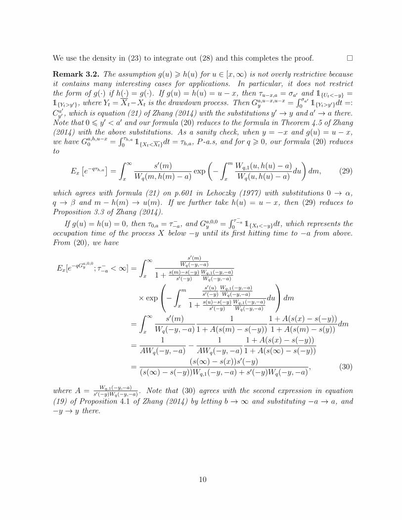
Remark 3.2. The assumption g(u) > h(u) for u ∈ [x,∞) is not overly restrictive becauseit contains many interesting cases for applications. In particular, it does not restrictthe form of g(·) if h(·) = g(·). If g(u) = h(u) = u − x, then τu−x,a = σa′ and 1Ut<−y =1Yt>y′, where Yt = X t−Xt is the drawdown process. Then Ga,u−x,u−x
y =∫ σa′0
1Yt>y′dt =:
Ca′
y′ , which is equation (21) of Zhang (2014) with the substitutions y′ → y and a′ → a there.Note that 0 6 y′ < a′ and our formula (20) reduces to the formula in Theorem 4.5 of Zhang(2014) with the above substitutions. As a sanity check, when y = −x and g(u) = u − x,we have Ga,h,u−x
0 =∫ τh,a0
1Xt<Xtdt = τh,a, P -a.s, and for q > 0, our formula (20) reducesto
Ex[e−qτh,a
]=
∫ ∞x
s′(m)
Wq(m,h(m)− a)exp
(−∫ m
x
Wq,1(u, h(u)− a)
Wq(u, h(u)− a)du
)dm, (29)
which agrees with formula (21) on p.601 in Lehoczky (1977) with substitutions 0 → α,q → β and m − h(m) → u(m). If we further take h(u) = u − x, then (29) reduces toProposition 3.3 of Zhang (2014).
If g(u) = h(u) = 0, then τ0,a = τ−−a, and Ga,0,0y =
∫ τ−−a0
1Xt<−ydt, which represents theoccupation time of the process X below −y until its first hitting time to −a from above.From (20), we have
Ex[e−qGa,0,0y ; τ−−a <∞] =
∫ ∞x
s′(m)Wq(−y,−a)
1 + s(m)−s(−y)s′(−y)
Wq,1(−y,−a)Wq(−y,−a)
× exp
−∫ m
x
s′(u)s′(−y)
Wq,1(−y,−a)Wq(−y,−a)
1 + s(u)−s(−y)s′(−y)
Wq,1(−y,−a)Wq(−y,−a)
du
dm
=
∫ ∞x
s′(m)
Wq(−y,−a)
1
1 + A(s(m)− s(−y))
1 + A(s(x)− s(−y))
1 + A(s(m)− s(y))dm
=1
AWq(−y,−a)− 1
AWq(−y,−a)
1 + A(s(x)− s(−y))
1 + A(s(∞)− s(−y))
=(s(∞)− s(x))s′(−y)
(s(∞)− s(−y))Wq,1(−y,−a) + s′(−y)Wq(−y,−a), (30)
where A = Wq,1(−y,−a)s′(−y)Wq(−y,−a) . Note that (30) agrees with the second expression in equation
(19) of Proposition 4.1 of Zhang (2014) by letting b → ∞ and substituting −a → a, and−y → y there.
10
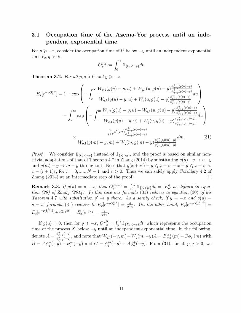
3.1 Occupation time of the Azema-Yor process until an inde-pendent exponential time
For y > −x, consider the occupation time of U below −y until an independent exponentialtime eq, q > 0:
Oq,gy :=
∫ eq
0
1Ut<−ydt.
Theorem 3.2. For all p, q > 0 and y > −x
Ex[e−pOq,gy ] = 1− exp
−∫ ∞x
Wq,2(g(u)− y, u) +Wq,1(u, g(u)− y)φ+′q+p(g(u)−y)φ+q+p(g(u)−y)
Wq,1(g(u)− y, u) +Wq(u, g(u)− y)φ+′q+p(g(u)−y)φ+q+p(g(u)−y)
du
−∫ ∞x
exp
−∫ m
x
Wq,2(g(u)− y, u) +Wq,1(u, g(u)− y)φ+′q+p(g(u)−y)φ+q+p(g(u)−y)
Wq,1(g(u)− y, u) +Wq(u, g(u)− y)φ+′q+p(g(u)−y)φ+q+p(g(u)−y)
du
×
pq+p
s′(m)φ+′q+p(g(m)−y)φ+q+p(g(m)−y)
Wq,1(g(m)− y,m) +Wq(m, g(m)− y)φ+′q+p(g(m)−y)φ+q+p(g(m)−y)
dm. (31)
Proof. We consider 1Ut<−y instead of 1Yt>y, and the proof is based on similar non-trivial adaptations of that of Theorem 4.7 in Zhang (2014) by substituting g(u)−y → u−yand g(m)− y → m− y throughout. Note that g(x+ iε)− y 6 x+ iε− x− y 6 x+ iε <x + (i + 1)ε, for i = 0, 1..., N − 1 and ε > 0. Thus we can safely apply Corollary 4.2 ofZhang (2014) at an intermediate step of the proof.
Remark 3.3. If g(u) = u − x, then Oq,u−xy =
∫ eq01Yt>y′dt =: Eq
y′ as defined in equa-tion (29) of Zhang (2014). In this case our formula (31) reduces to equation (30) of hisTheorem 4.7 with substitution y′ → y there. As a sanity check, if y = −x and g(u) =
u − x, formula (31) reduces to Ex[e−pOq,u0 ] = q
q+p. On the other hand, Ex[e
−pOq,u−x−x ] =
Ex[e−p
∫ eq0 1Xt<Xt
dt] = Ex[e−peq ] = q
q+p.
If g(u) = 0, then for y > −x, Oq,0−x =
∫ eq01Xt<−ydt, which represents the occupation
time of the process X below −y until an independent exponential time. In the following,
denote A =φ+′q+p(−y)φ+q+p(−y)
, and note that Wq,1(−y,m)+Wq(m,−y)A = Bφ+q (m)+Cφ−q (m) with
B = Aφ−q (−y) − φ−′q (−y) and C = φ+′q (−y) − Aφ+
q (−y). From (31), for all p, q > 0, we
11
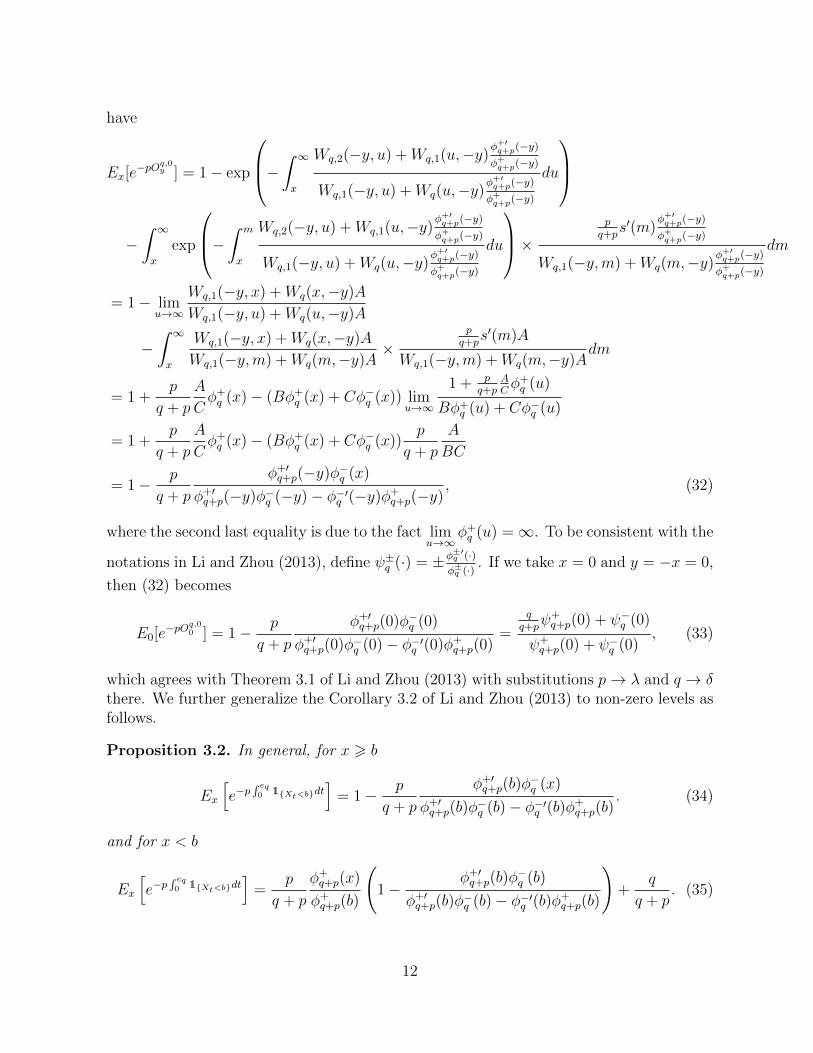
have
Ex[e−pOq,0y ] = 1− exp
−∫ ∞x
Wq,2(−y, u) +Wq,1(u,−y)φ+′q+p(−y)φ+q+p(−y)
Wq,1(−y, u) +Wq(u,−y)φ+′q+p(−y)φ+q+p(−y)
du
−∫ ∞x
exp
−∫ m
x
Wq,2(−y, u) +Wq,1(u,−y)φ+′q+p(−y)φ+q+p(−y)
Wq,1(−y, u) +Wq(u,−y)φ+′q+p(−y)φ+q+p(−y)
du
× pq+p
s′(m)φ+′q+p(−y)φ+q+p(−y)
Wq,1(−y,m) +Wq(m,−y)φ+′q+p(−y)φ+q+p(−y)
dm
= 1− limu→∞
Wq,1(−y, x) +Wq(x,−y)A
Wq,1(−y, u) +Wq(u,−y)A
−∫ ∞x
Wq,1(−y, x) +Wq(x,−y)A
Wq,1(−y,m) +Wq(m,−y)A×
pq+p
s′(m)A
Wq,1(−y,m) +Wq(m,−y)Adm
= 1 +p
q + p
A
Cφ+q (x)− (Bφ+
q (x) + Cφ−q (x)) limu→∞
1 + pq+p
ACφ+q (u)
Bφ+q (u) + Cφ−q (u)
= 1 +p
q + p
A
Cφ+q (x)− (Bφ+
q (x) + Cφ−q (x))p
q + p
A
BC
= 1− p
q + p
φ+′q+p(−y)φ−q (x)
φ+′q+p(−y)φ−q (−y)− φ−′q (−y)φ+
q+p(−y), (32)
where the second last equality is due to the fact limu→∞
φ+q (u) =∞. To be consistent with the
notations in Li and Zhou (2013), define ψ±q (·) = ±φ±′q (·)φ±q (·) . If we take x = 0 and y = −x = 0,
then (32) becomes
E0[e−pOq,00 ] = 1− p
q + p
φ+′q+p(0)φ−q (0)
φ+′q+p(0)φ−q (0)− φ−′q (0)φ+
q+p(0)=
qq+p
ψ+q+p(0) + ψ−q (0)
ψ+q+p(0) + ψ−q (0)
, (33)
which agrees with Theorem 3.1 of Li and Zhou (2013) with substitutions p→ λ and q → δthere. We further generalize the Corollary 3.2 of Li and Zhou (2013) to non-zero levels asfollows.
Proposition 3.2. In general, for x > b
Ex
[e−p
∫ eq0 1Xt<bdt
]= 1− p
q + p
φ+′q+p(b)φ
−q (x)
φ+′q+p(b)φ
−q (b)− φ−′q (b)φ+
q+p(b). (34)
and for x < b
Ex
[e−p
∫ eq0 1Xt<bdt
]=
p
q + p
φ+q+p(x)
φ+q+p(b)
(1−
φ+′q+p(b)φ
−q (b)
φ+′q+p(b)φ
−q (b)− φ−′q (b)φ+
q+p(b)
)+
q
q + p. (35)
12
Proof. For x > b, take y = −b > −x in (32), and we have the desired result in (34).For x < b, from the memoryless property of eq and the strong Markov property of X,
we have
Ex
[e−p
∫ eq0 1Xt<bdt
]= Ex
[e−pτ
+b ; τ+b < eq
]Eb
[e−p
∫ eq0 1Xt<bdt
]+ Ex
[e−peq ; eq < τ+b
]= Ex
[e−(q+p)τ
+b
]Eb
[e−p
∫ eq0 1Xt<bdt
]+
q
q + p
(1− Ex
[e−(q+p)τ
+b
]).
(36)
Then (35) follows from taking y = −b and x = b in equation (32) and Lemma 2.2 of Zhang(2014).
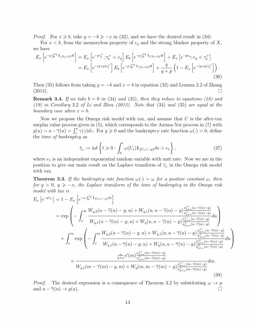
Remark 3.4. If we take b = 0 in (34) and (35), then they reduce to equations (18) and(19) in Corollary 3.2 of Li and Zhou (2013). Note that (34) and (35) are equal at theboundary case when x = b.
Now we propose the Omega risk model with tax, and assume that U is the after-taxsurplus value process given in (5), which corresponds to the Azema-Yor process in (7) withg(u) = u− γ(u) =
∫ uxγ(z)dz. For y > 0 and the bankruptcy rate function ω(.) > 0, define
the time of bankruptcy as
τω := inf
t > 0 :
∫ t
0
ω(Us)1Us<−yds > e1
, (37)
where e1 is an independent exponential random variable with unit rate. Now we are in theposition to give our main result on the Laplace transform of τω in the Omega risk modelwith tax.
Theorem 3.3. If the bankruptcy rate function ω(·) = ω for a positive constant ω, thenfor q > 0, y > −x, the Laplace transform of the time of bankruptcy in the Omega riskmodel with tax is
Ex[e−qτω
]= 1− Ex
[e−ω
∫ eq0 1Us<−yds
]= exp
−∫ ∞x
Wq,2(u− γ(u)− y, u) +Wq,1(u, u− γ(u)− y)φ+′q+ω(u−γ(u)−y)φ+q+ω(u−γ(u)−y)
Wq,1(u− γ(u)− y, u) +Wq(u, u− γ(u)− y)φ+′q+ω(u−γ(u)−y)φ+q+ω(u−γ(u)−y)
du
+
∫ ∞x
exp
−∫ m
x
Wq,2(u− γ(u)− y, u) +Wq,1(u, u− γ(u)− y)φ+′q+ω(u−γ(u)−y)φ+q+ω(u−γ(u)−y)
Wq,1(u− γ(u)− y, u) +Wq(u, u− γ(u)− y)φ+′q+ω(u−γ(u)−y)φ+q+ω(u−γ(u)−y)
du
×
ωq+ω
s′(m)φ+′q+ω(m−γ(m)−y)φ+q+ω(m−γ(m)−y)
Wq,1(m− γ(m)− y,m) +Wq(m,m− γ(m)− y)φ+′q+ω(m−γ(m)−y)φ+q+ω(m−γ(m)−y)
dm.
(38)
Proof. The desired expression is a consequence of Theorem 3.2 by substituting ω → pand u− γ(u)→ g(u).
13
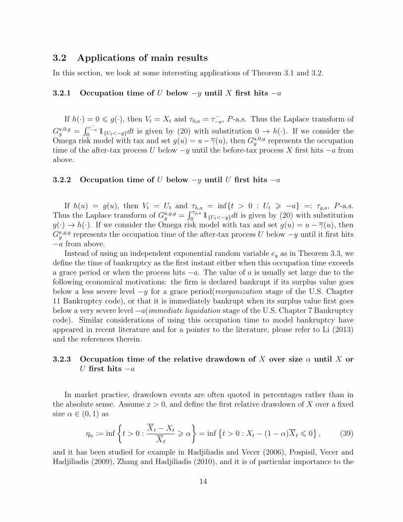
3.2 Applications of main results
In this section, we look at some interesting applications of Theorem 3.1 and 3.2.
3.2.1 Occupation time of U below −y until X first hits −a
If h(·) = 0 6 g(·), then Vt = Xt and τ0,a = τ−−a, P -a.s. Thus the Laplace transform of
Ga,0,gy =
∫ τ−−a0
1Ut<−ydt is given by (20) with substitution 0 → h(·). If we consider theOmega risk model with tax and set g(u) = u− γ(u), then Ga,0,g
y represents the occupationtime of the after-tax process U below −y until the before-tax process X first hits −a fromabove.
3.2.2 Occupation time of U below −y until U first hits −a
If h(u) = g(u), then Vt = Ut and τh,a = inft > 0 : Ut > −a =: τg,a, P -a.s.Thus the Laplace transform of Ga,g,g
y =∫ τg,a0
1Ut<−ydt is given by (20) with substitutiong(·)→ h(·). If we consider the Omega risk model with tax and set g(u) = u− γ(u), thenGa,g,gy represents the occupation time of the after-tax process U below −y until it first hits−a from above.
Instead of using an independent exponential random variable eq as in Theorem 3.3, wedefine the time of bankruptcy as the first instant either when this occupation time exceedsa grace period or when the process hits −a. The value of a is usually set large due to thefollowing economical motivations: the firm is declared bankrupt if its surplus value goesbelow a less severe level −y for a grace period(reorganization stage of the U.S. Chapter11 Bankruptcy code), or that it is immediately bankrupt when its surplus value first goesbelow a very severe level −a(immediate liquidation stage of the U.S. Chapter 7 Bankruptcycode). Similar considerations of using this occupation time to model bankruptcy haveappeared in recent literature and for a pointer to the literature, please refer to Li (2013)and the references therein.
3.2.3 Occupation time of the relative drawdown of X over size α until X orU first hits −a
In market practice, drawdown events are often quoted in percentages rather than inthe absolute sense. Assume x > 0, and define the first relative drawdown of X over a fixedsize α ∈ (0, 1) as
ηα := inf
t > 0 :
X t −Xt
X t
> α
= inf
t > 0 : Xt − (1− α)X t 6 0
, (39)
and it has been studied for example in Hadjiliadis and Vecer (2006), Pospisil, Vecer andHadjiliadis (2009), Zhang and Hadjiliadis (2010), and it is of particular importance to the
14
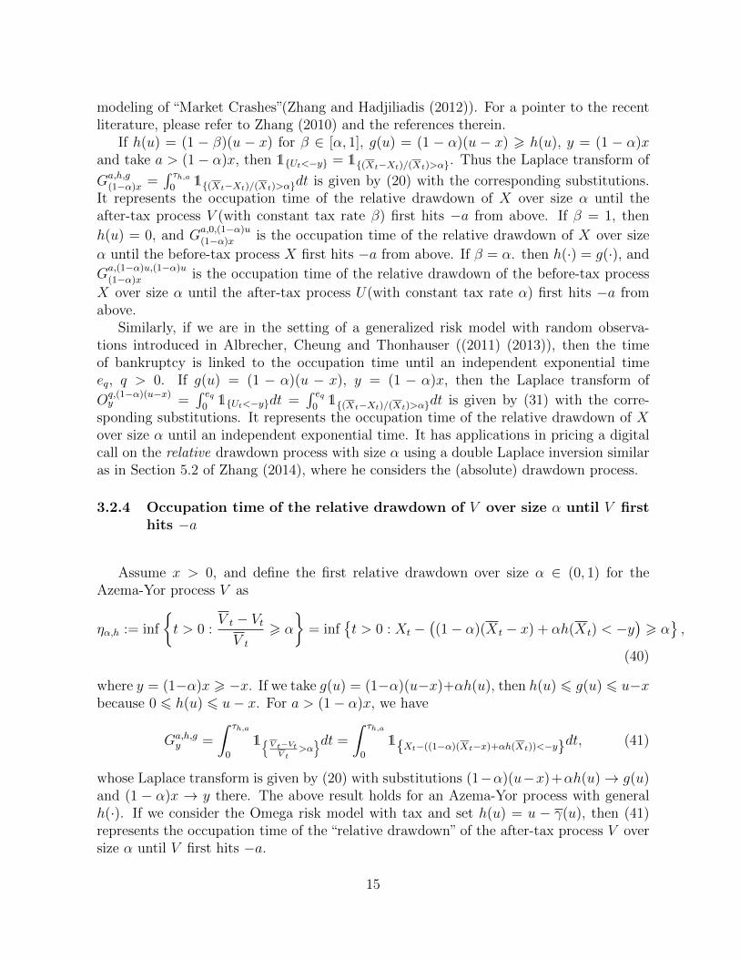
modeling of “Market Crashes”(Zhang and Hadjiliadis (2012)). For a pointer to the recentliterature, please refer to Zhang (2010) and the references therein.
If h(u) = (1 − β)(u − x) for β ∈ [α, 1], g(u) = (1 − α)(u − x) > h(u), y = (1 − α)xand take a > (1− α)x, then 1Ut<−y = 1(Xt−Xt)/(Xt)>α. Thus the Laplace transform of
Ga,h,g(1−α)x =
∫ τh,a0
1(Xt−Xt)/(Xt)>αdt is given by (20) with the corresponding substitutions.It represents the occupation time of the relative drawdown of X over size α until theafter-tax process V (with constant tax rate β) first hits −a from above. If β = 1, then
h(u) = 0, and Ga,0,(1−α)u(1−α)x is the occupation time of the relative drawdown of X over size
α until the before-tax process X first hits −a from above. If β = α. then h(·) = g(·), and
Ga,(1−α)u,(1−α)u(1−α)x is the occupation time of the relative drawdown of the before-tax process
X over size α until the after-tax process U(with constant tax rate α) first hits −a fromabove.
Similarly, if we are in the setting of a generalized risk model with random observa-tions introduced in Albrecher, Cheung and Thonhauser ((2011) (2013)), then the timeof bankruptcy is linked to the occupation time until an independent exponential timeeq, q > 0. If g(u) = (1 − α)(u − x), y = (1 − α)x, then the Laplace transform of
Oq,(1−α)(u−x)y =
∫ eq01Ut<−ydt =
∫ eq01(Xt−Xt)/(Xt)>αdt is given by (31) with the corre-
sponding substitutions. It represents the occupation time of the relative drawdown of Xover size α until an independent exponential time. It has applications in pricing a digitalcall on the relative drawdown process with size α using a double Laplace inversion similaras in Section 5.2 of Zhang (2014), where he considers the (absolute) drawdown process.
3.2.4 Occupation time of the relative drawdown of V over size α until V firsthits −a
Assume x > 0, and define the first relative drawdown over size α ∈ (0, 1) for theAzema-Yor process V as
ηα,h := inf
t > 0 :
V t − VtV t
> α
= inf
t > 0 : Xt −
((1− α)(X t − x) + αh(X t) < −y
)> α
,
(40)
where y = (1−α)x > −x. If we take g(u) = (1−α)(u−x)+αh(u), then h(u) 6 g(u) 6 u−xbecause 0 6 h(u) 6 u− x. For a > (1− α)x, we have
Ga,h,gy =
∫ τh,a
0
1V t−VtV t
>αdt =
∫ τh,a
0
1Xt−((1−α)(Xt−x)+αh(Xt))<−ydt, (41)
whose Laplace transform is given by (20) with substitutions (1−α)(u−x)+αh(u)→ g(u)and (1 − α)x → y there. The above result holds for an Azema-Yor process with generalh(·). If we consider the Omega risk model with tax and set h(u) = u − γ(u), then (41)represents the occupation time of the “relative drawdown” of the after-tax process V oversize α until V first hits −a.
15
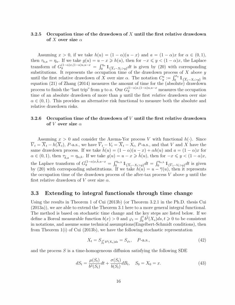
3.2.5 Occupation time of the drawdown of X until the first relative drawdownof X over size α
Assuming x > 0, if we take h(u) = (1 − α)(u − x) and a = (1 − α)x for α ∈ (0, 1),then τh,a = ηα. If we take g(u) = u− x > h(u), then for −x 6 y < (1− α)x, the Laplace
transform of G(1−α)x,(1−α)u,u−xy =
∫ ηα0
1Xt−Xt>ydt is given by (20) with correspondingsubstitutions. It represents the occupation time of the drawdown process of X above yuntil the first relative drawdown of X over size α. The notation Ca
y :=∫ σa01Xt−Xt>y in
equation (21) of Zhang (2014) measures the amount of time for the (absolute) drawdown
process to finish the “last trip” from y to a. Our G(1−α)x,(1−α)u,u−xy measures the occupation
time of an absolute drawdown of more than y until the first relative drawdown over sizeα ∈ (0, 1). This provides an alternative risk functional to measure both the absolute andrelative drawdown risks.
3.2.6 Occupation time of the drawdown of V until the first relative drawdownof V over size α
Assuming x > 0 and consider the Azema-Yor process V with functional h(·). SinceV t = X t − h(X t), P -a.s., we have V t − Vt = X t −Xt, P -a.s., and that V and X have thesame drawdown process. If we take h(u) = (1 − α)(u − x) + αh(u) and a = (1 − α)x forα ∈ (0, 1), then τh,a = ηα,h. If we take g(u) = u− x > h(u), then for −x 6 y < (1− α)x,
the Laplace transform of G(1−α)x,h,u−xy =
∫ ηα,h0
1Xt−Xt>ydt =∫ ηα,h0
1V t−Vt>ydt is givenby (20) with corresponding substitutions. If we take h(u) = u − γ(u), then it representsthe occupation time of the drawdown process of the after-tax process V above y until thefirst relative drawdown of V over size α.
3.3 Extending to integral functionals through time change
Using the results in Theorem 1 of Cui (2013b) (or Theorem 3.2.1 in the Ph.D. thesis Cui(2013a)), we are able to extend the Theorem 3.1 here to a more general integral functional.The method is based on stochastic time change and the key steps are listed below. If wedefine a Boreal measurable function b(x) > 0 and ϕt =
∫ t0b2(Xs)ds, t > 0 to be consistent
in notations, and assume some technical assumptions(Engelbert-Schmidt conditions), thenfrom Theorem 1(i) of Cui (2013b), we have the following stochastic representation
Xt = S∫ t0 b
2(Xs)ds= Sϕt , P -a.s., (42)
and the process S is a time-homogeneous diffusion satisfying the following SDE
dSt =µ(St)
b2(St)dt+
σ(St)
b(St)dBt, S0 = X0 = x. (43)
16
Let τ denote a Ft-stopping time of St, from Theorem 1(iii) of Cui (2013b), we have thatϕτ :=
∫ τ0b2(Xs)ds is a Gt-stopping time and τS = ϕτ , P -a.s., where τS is the corresponding
stopping time for St, and Gt = Fϕt .We have X t := max
06u6tXu = max
06u6tSϕu = max
06u6ϕtSu =: Sϕt , P -a.s., with the second
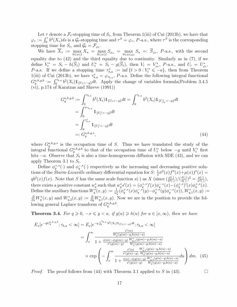
equality due to (42) and the third equality due to continuity. Similarly as in (7), if wedefine V ∗t = St − h(St) and U∗t = St − g(St), then Vt = V ∗ϕt , P -a.s., and Ut = U∗ϕt ,P -a.s. If we define a stopping time τ ∗h,a := inf t > 0 : V ∗t 6 −a, then from Theorem1(iii) of Cui (2013b), we have τ ∗h,a = ϕτh,a , P -a.s. Define the following integral functional
Ga,h,g,by :=
∫ τh,a0
b2(Xt)1Ut<−ydt. Apply the change of variables formula(Problem 3.4.5(vi), p.174 of Karatzas and Shreve (1991))
Ga,h,g,by :=
∫ τh,a
0
b2(Xt)1Ut<−ydt =
∫ τh,a
0
b2(Xt)1U∗ϕt<−ydt
=
∫ ϕτh,a
0
1U∗t <−ydt
=
∫ τ∗h,a
0
1U∗t <−ydt
=: Ga,h,g,∗y , (44)
where Ga,h,g,∗y is the occupation time of S. Thus we have translated the study of the
integral functional Ga,h,g,by to that of the occupation time of U∗t below −y until V ∗t first
hits −a. Observe that St is also a time-homogeneous diffusion with SDE (43), and we canapply Theorem 3.1 to St.
Define φ+,∗q (·) and φ−,∗q (·) respectively as the increasing and decreasing positive solu-
tions of the Sturm-Liouville ordinary differential equation for S: 12σ2(x)f ′′(x)+µ(x)f ′(x) =
qb2(x)f(x). Note that S has the same scale function s(·) as X (since ( µ(·)b2(·))/(
σ(·)b(·) )2 = µ(·)
σ2(·)),
there exists a positive constant w∗q such that w∗qs′(x) = (φ+,∗
q )′(x)φ−,∗q (x)−(φ+,∗q )′(x)φ+,∗
q (x).Define the auxiliary functionsW ∗
q (x, y) := 1w∗q
(φ+,∗q (x)φ−,∗q (y)−φ+,∗
q (y)φ−,∗q (x)), W ∗q,1(x, y) :=
∂∂xW ∗q (x, y) and W ∗
q,2(x, y) := ∂∂yW ∗q,1(x, y). Now we are in the position to provide the fol-
lowing general Laplace transform of Ga,h,g,by .
Theorem 3.4. For q > 0, −x 6 y < a, if g(u) > h(u) for u ∈ [x,∞), then we have
Ex[e−qGa,h,g,by ; τh,a <∞] = Ex[e
−q∫ τh,a0 b2(Xt)1Ut<−ydt; τh,a <∞]
=
∫ ∞x
s′(m)W ∗q (g(m)−y,h(m)−a)
1 + s(m)−s(g(m)−y)s′(g(m)−y)
W ∗q,1(g(m)−y,h(m)−a)W ∗q (g(m)−y,h(m)−a)
× exp
−∫ m
x
s′(u)s′(g(u)−y)
W ∗q,1(g(u)−y,h(u)−a)W ∗q (g(u)−y,h(u)−a)
1 + s(u)−s(g(u)−y)s′(g(u)−y)
W ∗q,1(g(u)−y,h(u)−a)W ∗q (g(u)−y,h(u)−a)
du
dm. (45)
Proof. The proof follows from (44) with Theorem 3.1 applied to S in (43).
17
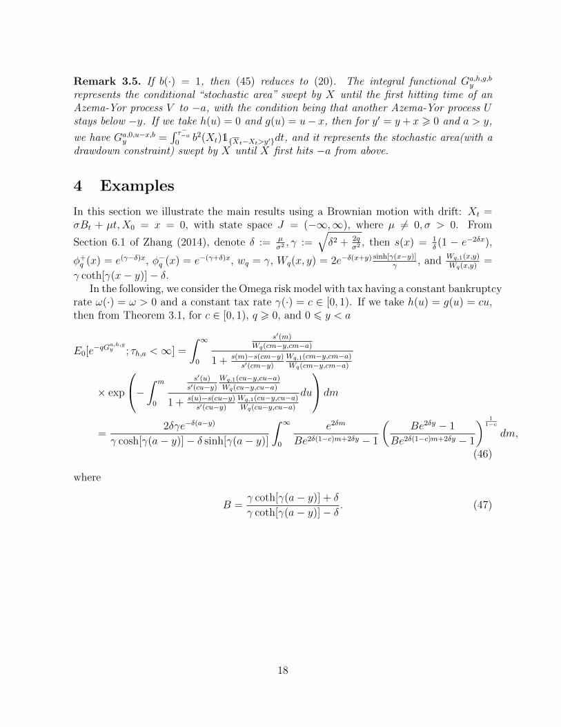
Remark 3.5. If b(·) = 1, then (45) reduces to (20). The integral functional Ga,h,g,by
represents the conditional “stochastic area” swept by X until the first hitting time of anAzema-Yor process V to −a, with the condition being that another Azema-Yor process Ustays below −y. If we take h(u) = 0 and g(u) = u− x, then for y′ = y+ x > 0 and a > y,
we have Ga,0,u−x,by =
∫ τ−−a0
b2(Xt)1Xt−Xt>y′dt, and it represents the stochastic area(with adrawdown constraint) swept by X until X first hits −a from above.
4 Examples
In this section we illustrate the main results using a Brownian motion with drift: Xt =σBt + µt,X0 = x = 0, with state space J = (−∞,∞), where µ 6= 0, σ > 0. From
Section 6.1 of Zhang (2014), denote δ := µσ2 , γ :=
√δ2 + 2q
σ2 , then s(x) = 1δ(1 − e−2δx),
φ+q (x) = e(γ−δ)x, φ−q (x) = e−(γ+δ)x, wq = γ, Wq(x, y) = 2e−δ(x+y) sinh[γ(x−y)]
γ, and Wq,1(x,y)
Wq(x,y)=
γ coth[γ(x− y)]− δ.In the following, we consider the Omega risk model with tax having a constant bankruptcy
rate ω(·) = ω > 0 and a constant tax rate γ(·) = c ∈ [0, 1). If we take h(u) = g(u) = cu,then from Theorem 3.1, for c ∈ [0, 1), q > 0, and 0 6 y < a
E0[e−qGa,h,gy ; τh,a <∞] =
∫ ∞0
s′(m)Wq(cm−y,cm−a)
1 + s(m)−s(cm−y)s′(cm−y)
Wq,1(cm−y,cm−a)Wq(cm−y,cm−a)
× exp
−∫ m
0
s′(u)s′(cu−y)
Wq,1(cu−y,cu−a)Wq(cu−y,cu−a)
1 + s(u)−s(cu−y)s′(cu−y)
Wq,1(cu−y,cu−a)Wq(cu−y,cu−a)
du
dm
=2δγe−δ(a−y)
γ cosh[γ(a− y)]− δ sinh[γ(a− y)]
∫ ∞0
e2δm
Be2δ(1−c)m+2δy − 1
(Be2δy − 1
Be2δ(1−c)m+2δy − 1
) 11−c
dm,
(46)
where
B =γ coth[γ(a− y)] + δ
γ coth[γ(a− y)]− δ. (47)
18
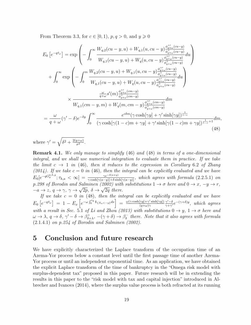
From Theorem 3.3, for c ∈ [0, 1), p, q > 0, and y > 0
E0
[e−qτω
]= exp
−∫ ∞0
Wq,2(cu− y, u) +Wq,1(u, cu− y)φ+′q+ω(cu−y)φ+q+ω(cu−y)
Wq,1(cu− y, u) +Wq(u, cu− y)φ+′q+ω(cu−y)φ+q+ω(cu−y)
du
+
∫ ∞0
exp
−∫ m
0
Wq,2(cu− y, u) +Wq,1(u, cu− y)φ+′q+ω(cu−y)φ+q+ω(cu−y)
Wq,1(cu− y, u) +Wq(u, cu− y)φ+′q+ω(cu−y)φ+q+ω(cu−y)
du
×
ωq+ω
s′(m)φ+′q+ω(cm−y)φ+q+ω(cm−y)
Wq,1(cm− y,m) +Wq(m, cm− y)φ+′q+ω(cm−y)φ+q+ω(cm−y)
dm
=ω
q + ω(γ′ − δ)e−δy
∫ ∞0
ecδm(γ cosh[γy] + γ′ sinh[γy])1
1−c
(γ cosh[γ(1− c)m+ γy] + γ′ sinh[γ(1− c)m+ γy])1
1−c+1dm,
(48)
where γ′ =√δ2 + 2(q+ω)
σ2 .
Remark 4.1. We only manage to simplify (46) and (48) in terms of a one-dimensionalintegral, and we shall use numerical integration to evaluate them in practice. If we takethe limit c → 1 in (46), then it reduces to the expression in Corollary 6.2 of Zhang(2014). If we take c = 0 in (46), then the integral can be explicitly evaluated and we have
E0[e−qGa,h,gy ; τh,a < ∞] = γe−δ(a+y)
γ cosh[γ(a−y)]+δ sinh[γ(a−y)] , which agrees with formula (2.2.5.1) on
p.298 of Borodin and Salminen (2002) with substitutions 1→ σ here and 0→ x, −y → r,−a→ z, q → γ, γ →
√2p, δ →
√2q there.
If we take c = 0 in (48), then the integral can be explicitly evaluated and we have
E0
[e−qτω
]= 1 − Ex
[e−ω
∫ eq0 1Xs<−yds
]= ω(γ cosh[γy]+γ′ sinh[γy])
(q+ω)γγ′−δγ+γ′
e−(γ+δ)y, which agrees
with a result in Sec. 5.1 of Li and Zhou (2013) with substitutions 0→ y, 1→ σ here andω → λ, q → δ, γ′− δ → β+
δ+λ, −(γ + δ)→ β−δ there. Note that it also agrees with formula(2.1.4.1) on p.254 of Borodin and Salminen (2002).
5 Conclusion and future research
We have explicitly characterized the Laplace transform of the occupation time of anAzema-Yor process below a constant level until the first passage time of another Azema-Yor process or until an independent exponential time. As an application, we have obtainedthe explicit Laplace transform of the time of bankruptcy in the “Omega risk model withsurplus-dependent tax” proposed in this paper. Future research will be in extending theresults in this paper to the “risk model with tax and capital injection” introduced in Al-brecher and Ivanovs (2014), where the surplus value process is both refracted at its running
19
maximum and reflected at zero. It would also be interesting to apply results in Section3.2 to designing new risk functionals taking into account both the absolute and relativedrawdown risks.
References
Albrecher, H., C. Cheung, and S. Thonhauser (2011): “Randomized observation periods for thecompound Poisson risk model: Dividends,” ASTIN Bulletin, 41(2), 645–672.
(2013): “Randomized observation periods for the compound Poisson risk model: the discountedpenalty function,” Scandinavian Actuarial Journal, (6), 424–452.
Albrecher, H., H. Gerber, and E. Shiu (2011): “The optimal dividend barrier in the Gamma-Omegamodel,” European Actuarial Journal, 1, 43–55.
Albrecher, H., and C. Hipp (2007): “Lundberg’s risk process with tax,” Bl. DGVFM, 28(1), 13–28.
Albrecher, H., and J. Ivanovs (2014): “Power identities for Levy risk models under taxation andcapital injections,” Stochastic Systems, forthcoming.
Albrecher, H., J. Renaud, and X. Zhou (2008): “A Levy insurance risk process with tax,” Journalof Applied Probability, 45(2), 363–375.
Azema, J., and M. Yor (1979): “Une solution simple au probleme de Skorokhod,” Seminaire de Prob-abilites, Springer, Berlin, 721, 90–115.
Borodin, A., and P. Salminen (2002): Handbook of Brownian motion-facts and formulae, 2nd edition.Birkhauser.
Cui, Z. (2013a): “Martingale property and pricing for time-homogeneous diffusion models in finance,”Ph.D. thesis, University of Waterloo.
(2013b): “Stochastic areas of diffusions and applications in risk theory,” working paper.
Gerber, H., and E. Shiu (1998): “On the time value of ruin,” North American Actuarial Journal, 2(1),48–72.
Gihman, I., and A. Skorohod (1972): “Stochastic differential equations,” Springer.
Hadjiliadis, O., and J. Vecer (2006): “Drawdowns preceding rallies in a Brownian motion model,”Quantitative Finance, 6(5), 403–409.
Karatzas, I., and S. Shreve (1991): “Brownian Motion and Stochastic Calculus,” Graduate Texts inMathematics. vol. 113, 2nd edn. Springer, New York.
Kyprianou, A., and R. Loeffen (2010): “Refracted Levy processes.,” Annales de l’Institut HenriPoincare, Probabilites et Statistiques, 46(1), 24–44.
Kyprianou, A., and X. Zhou (2009): “General tax structures and the Levy insurance risk model,”Journal of Applied Probability, 46(4), 1146–1156.
Landriault, D., J. Renaud, and X. Zhou (2011): “Occupation times of spectrally negative Levyprocesses with applications,” Stochastic Processes and their Applications, 121(11), 2629–2641.
(2014): “An insurance risk model with Parisian implementation delays,” Methodology and Com-puting in Applied Probability, forthcoming.
Lehoczky, J. (1977): “Formulas for stoopped diffusion processes with stopping times based on themaximum,” Annals of Probability, 5(4), 601–607.
20
Li, B. (2013): “Look-back stopping times and their applications to liquidation risk and exotic options,”Ph.D. Thesis, University of Iowa.
Li, B., Q. Tang, and X. Zhou (2013): “A time-homogeneous diffusion model with tax,” Journal ofApplied Probability, 50(1), 195–207.
Li, B., and X. Zhou (2013): “The joint Laplace transforms for diffusion occupation times,” Advancesin Applied Probability, 45(4), 1049–1067.
Louffen, R., J. Renaud, and X. Zhou (2014): “Occupation times of intervals until first passage timesfor spectrally negative Levy processes,” Stochastic Processes and their Applications, 124(3), 1408–1435.
Pospisil, L., J. Vecer, and O. Hadjiliadis (2009): “Formulas for stopped diffusion processes withstopping times based on drawdowns and drawups,” Stochastic Processes and their Applications, 119(8),2563–2578.
Protter, P. (2005): Stochastic integration and differential equations. Springer, 2nd edn.
Renaud, J. (2009): “The distribution of tax payments in a Levy insurance risk model with a surplus-dependent taxation structure,” Insurance Math. Econom., 45, 242–246.
(2014): “On the time spent in the red by a refracted Levy risk process,” Journal of AppliedProbability, forthcoming.
Zhang, H. (2010): “Drawdowns, drawups, and their applications,” Ph.D. Thesis, City University of NewYork.
(2014): “Occupation time, drawdowns, and drawups for one-dimensional regular diffusion,”Advances in Applied Probability, forthcoming, 17(1).
Zhang, H., and O. Hadjiliadis (2010): “Drawdowns and rallies in a finite time-horizon,” Methodologyand Computing in Applied Probability, 12(2), 293–308.
(2012): “Drawdowns and the speed of a market crash,” Methodology and Computing in AppliedProbability, 14(8), 739–752.
21


