On comparing biological shapes: Detection of influential landmarks

AMERICAN JOURNAL OF PHYSICAL ANTHROPOLOGY 8749-65 (1992)

On Comparing Biological Shapes: Detection of Influential Landmarks

SUBHASH LELE AND JOAN T. RICHTSMEIER Department of Biostatistics, School of Hygiene and Public Health (S.L.), and Department of Cell Biology and Anatomy, School of Medicine (J.T.R.), Johns Hopkins University, Baltimore, Maryland 21205

KEY WORDS Euclidean distance matrix, Local form change, Morphology, Sexual dimorphism, Macaca fascicularis, Apert syndrome

ABSTRACT For problems of classification and comparison in biological research, the primary focus is on the similarity of forms. A biological form consists of size and shape. Several approaches for comparing biological forms using landmark data are available. If the two biological forms are demon- strated to be different, the next important issue is to localize the differences by identifying those areas which differ most between the two objects. In this paper we suggest a technique to detect influential landmarks, those which contribute most to the difference between forms. We study the effectiveness of the technique using three-dimensional simulated data sets and two examples. Results suggest that the technique is useful in the study of biological form and its variation.

An inevitable result of biological processes such as growth, evolution, or teratological mechanisms is change in form of the object under study. Form of an object consists of both size and shape.

Most biological forms contain identifiable loci which are referred to as biological landmarks. To be of analytical use, they must be present on all specimens under consideration. Landmark data are the coordinates of these biological loci. Thus for a three-dimensional form with k landmarks, we have a k x 3 matrix of coordinates (see Bookstein (19861, Goodall and Bose (19871, Lele (1991), Lele and Richtsmeier (1991), and Lewis et al. (1980) for more discussion on landmark data and analysis). In this paper we assume that such data are available.

We note here that landmark data alone do not provide all information pertaining to the form of the object. For example, the curva- ture of surfaces between landmarks could be important. However, methods that utilize landmark and outline data simultaneously are not available at present. In the remaining part of the paper we accept this limita- tion of landmark data and proceed to exploit all pertinent information from this type of

data. Thus whenever we say form of an object, we mean the form as represented by landmark data.

Suppose XI, X,, . . . X,, arethe individuals from population X and Y,, Y,, . . . Y, are the individuals from population Y. Here Xi (or YJ denotes the k x 3 or kx2 matrix of landmark coordinates. Further, let us suppose that using any of the morphometric techniques currently available we conclude that populations X and Y have different shapes. The problem we wish to address in this paper is how to determine which parts, or landmarks, of objects X and Y account for the majority of the morphological differences between X and Y. Is it possible to rank the parts according to their contribution to the defined shape or form difference?

Often the biologist has expectations about those loci or regions that differ most between two forms. The proposed method can be used to test such biologically based hypotheses. The biologist’s input is crucial to the intelli- gent formulation of such hypotheses.

In some situations, the difference between

Received July 31,1989; accepted February 13,1991.

@ 1992 WILEY-LISS, INC.

50 S. LELE AND J.T. RICHTSMEIER

populations of forms may not be explainable by any current theory. In this case, statistical methods can be used to explore possibili- ties not yet considered by the biologist. In this paper we also demonstrate how Euclid- ean Distance Matrix Analysis (EDMA) proposed by Lele (1991) and Lele and Richts- meier (1991) enables one to explore possible areas of morphological differences. “Statisti- cal exploration” for influential landmarks can be important scientifically, but biological knowledge ultimately is necessary for understanding and explaining the differences.

This paper begins with a brief description of EDMA. We then describe a method for identifying the possible loci of morphological differences between forms, and a technique for ranking the areas according to their influence. We present a small simulation study using artificial data in three dimensions to justify and judge the performance of our suggested method. Finally, we include analyses of two biological data sets and offer explanations for the analytical results obtained using knowledge of the biological sys- tems under consideration.

EUCLIDEAN DISTANCE MATRIX ANALYSIS-A BRIEF REVIEW

In this section we give a brief introduction to Euclidean Distance Matrix Analysis (EDMA). Interested readers should consult Lele (1991) and Lele and Richtsmeier (1991) for a more detailed explanation.

Let the given object be either two-dimensional or three-dimensional with k landmarks. This object can be represented by a kx 2 or kx 3 matrix of landmark coordinates. A coordinate-free representation of this object, (i.e., a representation which is invariant under translation, rotation, and reflection) is given in terms of a Euclidean distance matrix (see Mardia et al. (1979), Chapter 14, for details). The Euclidean distance matrix is a symmetric matrix of dimension k x k with the (ijIth entry corresponding to the distance between landmarks i and j. Since this matrix contains information on both size and shape, we call this a form matrix and denote it by F.

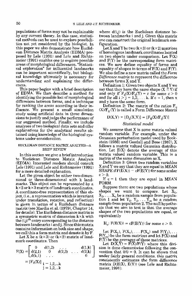
Let X be a (kx3) or (kx2) matrix of landmark coordinates. Then

F(X) = d(2,l) 0 d(2,3) . . . d(2,k)I 0 d(1,2) . . . d(1,k)

d(k,l) . . . 0

k , ,...

[ = [Fij(X)I i = 1 2

j = 1,2, ... k

where d(ij) is the Euclidean distance between landmarks i and j. Given this matrix one can construct the original landmark con- figuration.

Let XandY be two (kx 3) or (kx2) matrices of homologous landmark coordinates located on two objects under comparison. Let F(X) and F(Y) be the corresponding form matrices. We now define equality of forms and equality of shapes in terms of F(X) and F(Y). We also define a new matrix called the Form Difference matrix to represent the difference between forms X and Y.

Definition 1: Given two objects X and Y we say that they have the same shape (X Y) if and only if Fij(X>/Fij(Y) = c for some c > 0 and for all i > j = 1,2, . . . k. If c = 1, then x and y have the same form.

Definition 2: The matrix of the ratios F, (X)/Fij (Y) is called a Form Difference Matrix

D(X,Y) = [Dij(X,Y)I = [Fij(X)/Fij(Y)I Statistical model

We assume that X is some matrix valued random variable. For example, under the Gaussian perturbation model used by Book- stein (1986) and Goodall and Bose (19871, X follows a matrix valued Gaussian distribution. Let E(X) denote the average of this matrix valued random variable. This is a matrix of the same dimension as X.

Definition 3: Given two random variables X and Y we say that they are equal in MEAN SHAPE if F(E(X)) = cF(E(Y)) for some scalar c > 0.

If-c = 1 then they are equal in MEAN FORM.

Suppose there are two populations whose shapes we want to compare. Let XI, X,, . . . X, be a random sample from population 1 and let Y,, Y2,. . . Y, be a random sample from population 2. The null hypothesis that we aim to test is that the average shapes of the two populations are equal, or equivalently

H,: F(E(X)) = cF(E(Y)) for some c > 0.

Let F(X,), F(X2), . . . F(XJ and F(&), . . . F(I7-J be the form matrices and let F(X) and F(Y) be th__ee_average_s of 3 e s e matrices.

Let D(X,Y) = F(X)/F(Y) where this divi- sion is done elementwise following the con- vention that 0/0 = 0. It can be shown that under fairly general conditions, this matrix consistently estimates the form difference matrix D(E(X), E(Y)) (see Lele and Richts- meier, 1991).

LOCALIZING SHAPE CHANGE 51

- Let Dij (X,y) be the (ijIth element of DCX, Y). The test statistic we use to test the null hypothesis is

Tabs = max Dij (X, Y)/min Dij (X, q). i>j i>j

If this test statistic is “significantly” larger than 1, we reject the null hypothesis. We use a bootstrap procedure to estimate the null distribution and the p-value. If the p-value is small, we reject the null hypothesis.

If after testing for the similarity of shapes, the two objects seem to be different, the next issue is localization of the differences. In the following s&on we use the form difference matrix D(X,Y) to detect influential landmarks and then suggest a technique to rank areas according to their influence.

DETECTION OF INFLUENTIAL LANDMARKS

There are two steps involved in the detec-

Step 1. Use the form difference matrix and biological knowledge of the forms being compared to suggest possible areas of influence.

Step 2. Rank these areas according to their influence on the differentiation of forms.

tion of influential landmarks:

We now offer a detailed description of these steps.

Step 1 Consider the form difference matrix for

two objects X and Y.

D(X,Y) = Fij(X)/Fij(Y) = Dij(X,Y)

If Fij(X)/Fij(Y) is less than 1, the distance between landmarks i and j is shorter in X than in Y or equivalently, X has decreased with respect to Y. Similarly if this ratio is larger than 1, X has increased with respect to Y.

Landmarks which are involved in ratios that are “substantially smaller” or “substantially larger” than 1 are instrumental in determining form difference. If these landmarks combine to form a biologically relevant part of the object, that part is considered influential. One can simply look at the form difference matrix ordered according to the value of the ratios. Those landmarks that are involved in the extremes, either low or high, should be studied further for their biological relevance.

Step 2 It is reasonable that the landmarks which

appear at the extremes of Dij(X,Y) may con- stitute two different parts of the object. We need to rank them according to their influence. Our procedure for ranking is based on the following logic: the closer the value of Tobs is to 1, the more congruent are the objects.

If a particular part of the object is responsible for a majority of the form difference, deletion of that part of the object should result in an improved match of the forms defined by the remaining landmarks. One can thus rank the influence of a particular set of landmarks by observing the reduction in Tabs caused by deleting that particular set. The larger the reduction, the larger is the influence.

Two concerns should be noted when applying this logic in practice.

1. The values of T are not directly comparable. We need to calibrate them. We use p-values toward this objective. After deletion of landmarks, a substantial increase in the p-value indicates substantial influence of the deleted landmarks.

2. Some weight should be given to the number of landmarks deleted. If a smaller set of landmarks achieves a reduction in T (or increase in the p-value) similar to that achieved by a larger set, the smaller set is more influential.

Unfortunately there seems to be no objective way of combining the two features. The procedure we suggest is the following:

Step 1. Arrange the form difference matrix in an increasing order. Consider the set of landmarks that are involved in the extrema of the matrix.

Step 2. Group these landmarks in a biologically sensible manner. Let A,, A,, . . . A, be groups that can be formed using landmarks that appear at the extremes.

Step 3. Calculate TA,, T4, . . . TAP where T4 is the value of T after deleting 4, and the corresponding p-values.

Step 4. Use the rule “larger the p-value, larger the influence” to rank A, . . . Aa, but also consider the number of landmarks in each set. The general rule is that if a smaller set of landmarks causes a decrease in Tohs (or similar increase in the p-value) similar to that produced by a larger set, then the smaller set is more influential.


In regression analysis, Cook (1977) uses a similar idea to study influential observations. Following Cook’s approach, one may delete one landmark at a time to study the influence of an individual landmark. How- ever, as in regression analysis, this procedure involves a masking effect. It is not uncommon for two or more landmarks to be influential when considered together, but to have minimal influence when considered in- dividually.

When prior knowledge about the possible influential areas is lacking, the following strategy may be used:

1. Divide the object into mutually exclu- sive and exhaustive parts in a biologically sensible manner, say Al, A,, . . . Ap.

2. Use the above procedure to rank their influence.

One can use D(x,Y) in Step 1 but it is not necessary.

DATA ANALYSIS

In this section, we demonstrate how the above procedure can be used to analyze bio- logicaldata. First, we study the performance of the procedure on simulated data sets where the truth is known. We believe that if a procedure leads us to correct conclusions in simulations, we can be confident in applying the method to real data sets and in using the results to explain morphological differences.

Simulated data sets We use a perturbation model to generate

random three-dimensional figures. Our average 3-D forms (E(X) and E(Y)) consist of eight landmarks with coordinates:

E(X) =

E(Y) =

0 0 0- 1 0 0 1 1 0 0 1.3 0 0 0 1 1 0 1 1 1 1 0 1 1 -

(See Fig. 1.) Our hypothetical forms are identical except local to landmark 4 (Figure 1). The form difference matrix that represents the true form difference between E(X) and E(Y) is presented in Table 1 of the Appendix.

To generate observations we used the following perturbations: Landmarks 1 and 5 were not perturbed at all. Error distribution was degenerate at 0. Landmarks 2 and 6 were perturbed according to a Gaussian distribution with mean 0 and variance matrix u21 with u = 0.1. Landmarks 3 and 7 were perturbed according to a uniform distribution with range (-0.2, 0.2) on each axis. Landmarks 4 and 8 were perturbed with a distribution a(X - 1) where X follows an ex- ponential distribution with mean 1 and a = 0.1. Note that the perturbation distribu- tions are nonidentical and nonsymmetric.

We generated samples of different sizes:

Population X Population Y n = 10 m = 6 n = 20 m = 5 n = 30 m = 30

These represent small, medium, and large sample sizes realistically encountered in biological research. The experiment was re- peated 10 times for each sample size. An example of an ordered form difference matrix produced from each of these studies is presented in Table 2 of the Appendix. The 10 ordered form difference matrices for the three studies are available upon request. Inspecting this table, we observe that:

1. For large sample sizes, the estimated form difference matrix mimics the true form difference matrix (Table 1) closely. ThisSE- roborates empirically the result that D(X,Y) estimates D(E(X),E(Y)) consistently.

2. For smaller samples, this relation is not very close. However, landmark 4, the influential landmark, does occur in the extremes with high frequency.

Table 3 of the Appendix provides the p- values obtained after deleting each of the landmarks. We observe that the rule “larger the p-value, larger the influence” does lead us to the influential landmark (landmark 4) consistently.

In summary, our simulation indicates that the ordered form difference matrix and “delete a landmark technique work well for realistic sample sizes.


TABLE 1 . Three-dimensional landmarks used in analvsis of Macaca fascicularis

Fig. 1. Three-dimensional hypothetical forms used in simulation study. Landmark 4 is changed from (0,1,0) to (0,1.3,0). All other landmarks remain the same in both the figures.

Example 1: Sexual dimorphism in Macaca fascicularis

Mechanisms proposed to explain sexual dimorphism in primates remain diverse, and there is no consensus regarding the primacy of the processes responsible for dimorphism (see Kay et al., 1988; Leutenegger and Kelly, 1977; Cheverud et al., 1985). Following others (see Shea, 1983, 19891, we are particularly interested in the role of ontogenetic mechanisms in the production of dimorphism. EDMA's capability to determine those loci that differ most (or least) between the sexes at various stages of the growth process can help us to define differences in morphological patterns, and propose specific ontogenetic mechanisms responsible for sexual dimorphism of adult forms.

Because the generalized macaque morphology is familiar to readers and much work has been done regarding sexual dimorphism of primates (e.g., Schultz, 1962; Ikeda and Wanatabe, 1966; Albrecht, 1978; Chev- erud and Richtsmeier, 19861, we use three- dimensional coordinate data from biological landmarks located on the skulls of Macaca fascicularis to examine the use of EDMA in the study of ontogeny of sexual dimorphism in this species. The M . fascicularis skulls come from the collections of the National Museum of Natural History, the Smithson- ian Institution. Most specimens are wild shot and sex was recorded at the time of collection. Individual monkeys were placed in developmental age categories based on tooth eruption patterns. For the example

Landmark number Landmark name and description

1

2

3

4

5

6

7

8

9

10

11

12

13

14

15

16

17

18

Point located midway along the arc measured along the neurocranial surface from bregma to nasion.

Nasion. Point of intersection of the nasal bones with the frontal bone.

Nasale. Inferior-most point of intersection of the nasal bones.

Intradentale superior. The point is located on the alveolar border of the maxilla between the central incisors.

Right junction of premaxilla and maxilla on alveolar surface.

Left junction of premaxilla and maxilla on alveolar surface.

Right junction of the frontal bone with the zygomatic bone on the orbital rim.

Left junction of the frontal bone with the zygomatic bone on the orbital rim.

Right zygomaxillare superior. Intersection of zygomatic bone and maxilla at the inferior orbital rim.

Left zygomaxillare superior. Intersection of zygomatic bone and maxilla a t the inferior orbital rim.

Right pterion posterior. Intersection of the frontal, sphenoid, and temporal bones.

Left pterion posterior. Intersection of the frontal, sphenoid, and temporal bones.

Right maxillary tuberosity. Intersection of the maxilla and the palatine bones.

Left maxillary tuberosity. Intersection of the maxilla and the palatine bones.

Intersection of the zygomatic, maxillary, and sphenoid bones at the pterygo-palatine fossa on the right side.

Intersection of the zygomatic, maxillary, and sphenoid bones at the pterygo- palatine fossa on the left side.

Posterior nasale spine. Intersection of vomer and palatine bones at midline palate.

Junction of the vomer and sphenoid bone on the sphenoid body.

presented here we chose to analyze a region of the craniofacial complex that has been shown by others (e.g., Cheverud and Richts- meier, 1986) to experience extensive growth and to show marked dimorphism.

From a total of 45 landmarks identified on the faces of M . fascicularis, eighteen were selected (see Table 1, Figure 2) to adequately describe a single anatomical region of the craniofacial skeleton. The region is defined as the face (excluding the mandible) including its sites of attachment to the basicra- nium and neurocranium. Landmark locations were recorded using the Polhemus


A

C

B Fig. 2.

Table 1. Landmarks located on facial skeleton of M. fusciculuris. Landmark definitions are listed in

Navigation 3Space electromagnetic digitizer that records locations in three dimensions with a resolution of .8 millimeters and a high degree of accuracy.

We use the two extreme age categories in our example: developmental age 1 contains only individuals with a complete deciduous dentition, while developmental age 5 contains only individuals with a complete adult dentition. We compare male and female facial morphologies within and between developmental age categories 1 and 5 to identify those regions of the face which are most

sexually dimorphic in immature and adult individuals. Results enable us to make infer- ences about the way in which sexual dimorphism of facial growth contributes to adult sexual dimorphism.

This example is presented to demonstrate the usefulness of EDMA in biological studies. Properties specific to the method (e.g., three-dimensionality) produce results that are not directly comparable to results obtained from most other methods. However, we have shown elsewhere (Richtsmeier and Lele, 1990) that results obtained from


EDMA and from finite-element scaling analysis (FESA) are similar. To establish whether EDMA provides biologically meaningful results in this example, we compare results of this EDMA of sexual dimorphism in M. fascicularis to results of a FESA of sexual dimorphism in M. mulatta (Cheverud and Richtsmeier, 1986). We have formulated several hypotheses concerning sexual dimorphism of growth of the generalized macaque face from data presented by Cheverud and Richtsmeier (1986). That study is well suited for comparison with our example because 1) there is a good deal of similarity in facial morphology and growth between M. fascicularis and M. mulatta (Richtsmeier and Chev- erud, 1989); 2) many of the landmarks used by Cheverud and Richtsmeier (1986) are used here; and 3) the analytical method used by Cheverud and Richtsmeier (1986) (FESA) is three-dimensional enabling a direct comparison of results of EDMA and FESA. Our working hypotheses formulated from results presented by Cheverud and Richtsmeier (1 986) include:

Ho,. There is little sexual dimorphism in the youngest age group (developmental age 1). Minimal sexual differences in shape exist and local size differences indicate that males are neither predominantly larger nor smaller than females.

Ho,. The pattern of growth is similar in the two sexes.

Ho,. Males grow faster than females.

The following example is not designed to be a comprehensive test of our hypotheses, but it allows evaluation of our EDMA results as they relate to these hypotheses to determine if general agreement exists between the two studies. If agreement exists, we conclude that EDMA provides biologically meaningful results.

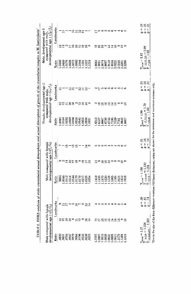
We first compared male to female facial morphology within the youngest and oldest age groups using the males as the base sample (numerator). For developmental age 1 there are 12 males and 3 females, while developmental age 5 consists of 36 males and 20 females. We realize that the sample sizes for developmental age 1 are small, but not unusually so for anthropological, clinical, or paleontological studies.

The form difference matrix D(X,Y), where X is the male sample (developmental age 1) and Y the female sample (developmental age

11, is presented in the first column of Table 2. Differences in shape between the sexes are not statistically significant at this age. The form difference matrix is symmetrically dis- tributed around 1 indicating that males are neither generally larger nor smaller than females at this age. Hypothesis 1 is confirmed by our analysis.

Details of sexual dimorphism in shape at developmental age 1 can be evaluated by a careful inspection of the form difference matrix. Focusing on the upper end of the matrix (smaller ratios), it is evident that linear distances oriented across the face (especially those including zygomaxillare superior) contribute to a larger nasal complex in the female face. The anterior portion of the alveolus, including the most anterior portion of the maxilla and the premaxilla is larger in males. Specific palatal loci (premaxilla-maxilla intersection, intradentale superior) in combination with other facial and palatal landmarks indicate a longer palate (measured along the AP axis) and generally larger snout in males at this early age. For example, zygomaxillare superior in combination with the premaxillary-maxillary intersection produces measures which are much greater in males. These localized results are in general agreement with those presented by Cheverud and Richtsmeier (1986, Tables 2 and 4).

To determine those loci that contribute most to facial sexual dimorphism at developmental age 1, we performed our proposed procedure for the detection of influential landmarks. Inspection of the form difference matrix (Table 2) indicates that left and right premaxilla-maxilla intersection and intradentale superior (4,5,6) aggregate at one end of the form difference matrix and therefore contribute most to differences in shape between the sexes at developmental age 1. There is no biologically meaningful group of landmarks that accounts for the linear distances at the minimum end of the matrix. Our goal is to change the composition of the form difference matrix by deleting the fewest number of landmarks. This is done most efficiently in this particular case by focusing on the maximal of the matrix.

When landmarks 4, 5, and 6 are deleted and the analysis is rerun, the p-value increases to .81 (Table 2). This jump in the p-value delineates a great similarity between male and female facial shape at this developmental age when the anterior-most

TAB

LE 2

. E

DM

A a

naly

sis

of s

tatic

cra

niof

acia

l sex

ual d

imor

phis

m a

nd s

exua

l dim

orph

ism

of

grow

th o

f the

cra

niof

acia

l com

plex

in M

. fas

cicu

lari

s'

Mal

e, d

evel

opm

ent a

ge 5

deve

lopm

enta

l age

1 (85/81)

Fem

ale,

dev

elop

men

tal a

ge 5

deve

lopm

enta

l ag

e 1 (9

5/8J

M

ale

com

pare

d w

ith fe

mal

e M

ale

com

pare

d w

ith fe

mal

e co

mpa

red

with

mal

e,

com

pare

d w

ith m

ale,

de

velo

pmen

tal a

ge 1

(dl/

Q1)

de

velo

pmen

tal

age

5 (&/Q,)

Rat

io

Lan

dmar

ks

Rat

io

Lan

dmar

ks

Rat

io

Lan

dmar

ks

Rat

io

Lan

dmar

ks

3622

10

9

.998

4 9

7 1.

0093

12

11

1.

0486

12

1

__

_

~ _

__

3651

15

11

.8

704

18

17

.884

7 10

2

3979

9

2 .g

o58

11

10

.910

6 10

7

.921

6 9

8

.004

8 2

1 1.

0184

12

1

1.04

89

12

11

,011

2 14

13

1.

0232

11

1

1.05

78

2 1

,011

4 10

1

1.04

69

16

11

1.06

08

11

1

,014

4 17

13

1.

0494

16

15

1.

0673

16

15

,0

170

16

15

1.05

28

2 1

1.08

92

16

11

,017

9 9

1 1.

0645

15

12

1.

1044

15

12

,0

217

16

1 1.

0659

18

11

1.

1184

18

11

.9

239

16

12

1.02

25

17

14

1.08

39

18

12

1.12

22

16

1

.925

3 18

14

1.

0254

10

8

1.09

21

8 1

1.12

24

8 1

1.07

07

10

4 1.

1419

13

5

1.65

13

3 2

1.86

83

18

17

1.08

07

17

4 1.

1430

9

6 1.

6537

18

17

1.

9021

15

5

1.08

15

15

5 1.

1470

10

5

1.66

67

15

5 1.

9074

16

6

1.08

29

15

4 1.

1530

10

3

1.67

38

16

6 1.

9097

3

2 1.

0831

13

4

1.15

38

10

4 1.

6742

13

5

1.91

18

13

5 1.

0898

14

4

1.09

15

16

4 1.

1079

16

6

1.15

65

3 2

1.15

68

9 4

1.16

16

9 3

1.71

95

14

6 1.

7529

10

4

1.77

61

9 4

1.95

24

14

6 2.

0225

10

4

2.05

46

9 4

1.15

68

9 5

1.18

52

10

6 1.

8643

9

5 2.

2291

10

6

1.18

18

10

6 1.

1959

9

5 1.

8807

10

6

2.22

96

9 5

Tto

tal =

1.3

7 p

= .2

8 T

bt31

= 1

.198

p

= .0

1 Tt

,,t31 =

1.8

6 p

= .0

1 Tt

,,t31 =

2.1

2 p

= .0

1 T

-(4,

5,3 =

1.2

38

p =

.81

T-(

3,4,

5,6)

=

p

= .1

8 T

-(l,

ll,l

Z) =

1.7

9 p

= .O

1 T

-(1,

11,1

2) =

2.0

9 p

= .0

1 T

-(,,,

,,,g,

io) =

1.2

31

p =

.74

T-(

g.~o

) = 1

.151

p

= .1

4 T

-(4,

5,5)

= 1

.64

p =

.01

T-(

i 5 6)

= 1

.82

p =

.01

'Due

to th

e si

ze o

f th

e fo

rm d

iffer

ence

mat

rice

s (15

3 lin

ear

dist

ance

s), r

atio

s ar

e sh

own

for

the

min

imum

and

max

imum

ext

rem

a on

ly.


landmarks on the alveolus are excluded from analysis. Landmarks on the anterior palate are responsible for the small degree of sexual dimorphism present in the face of immature Macaca fascicularis. Landmarks 9 and 10 (left and right zygomaxillare superior) appear at both ends of the new form difference matrix; however, deleting them from the analysis does not change the p-value substantially, and the decrease in value of the newly calculated T is trivial. Note, however, that these landmarks in combination with those on the anterior alveolus were at the maximum of the original form difference matrix for this age group.

Comparison of facial morphology between the sexes for developmental age group 5 is found in column 2, Table 2. The form difference matrix is obviously skewed towards ratios greater than one indicating a global magnification of the male form as compared to the female. Only one linear distance is actually larger in the females, but this ratio is very close to 1. Like the form difference matrix for developmental age 1, ratios a t the minimum end of the matrix represent combi- nations of many landmarks with no specific region represented. There is a distinct pattern at the maximum end of the matrix, however.

Landmarks located along the anterior alveolus (intradentale superior, and premaxilla-maxilla intersection) cluster at the maximum end of the matrix just as they did in the analysis of developmental age 1, and the two linear distances representing the max- ima of the form difference matrix are identical for the two age groups studied. This indicates that midfacial height measured from premaxilla-maxilla to zygomaxillare superior is the most sexually dimorphic dimension of facial shape in the youngest age group, and remains that way in the adult. Since the ratios comparing male to female linear distances among these landmarks are not greatly different between the younger and older age groups, we suspect that sexually dimorphic growth vectors for this area of the face (after the eruption of the deciduous dentition) are not responsible for the ontogenetic continuation of the documented sexual dimorphism. Instead, this local dimorphism is established prenatally, or early during the post-natal months and similar localized growth trends in the two sexes maintain the established pattern. Unlike the younger age group, however, nasale appears at the maximum extreme of the developmental age 5

matrix in combination with zygomaxillare superior and nasion. We suggest that sexual dimorphism in growth local to nasale is in part responsible for adult sexual dimorphism of the M. fascicularis snout.

In our attempt to detect the influential landmarks, we note that deletion of landmarks 9 and 10 produces a T that is not much greater than that calculated for landmarks 3,4 ,5 , and 6. This indicates that zygomaxillare superior (in combination with other facial landmarks) accounts for a large degree of sexual dimorphism of adult M. fascicularis faces.

To mimic the design of the growth comparisons done by Cheverud and Richtsmeier (1986), we compared the developmental age 1 male sample with the developmental age 5 male and female samples. These comparisons inform us of how the adult male and female forms differ from the immature male form and allow evaluation of sexual dimorphism of facial growth. The adult form was used as the base sample (numerator) in the two comparisons. The form difference matrices are presented in Table 2 (columns 3 and 4).

The form difference matrices for the comparison of the immature male sample to the adult male sample and to the adult females are nearly parallel. Nine of the 10 linear distances in the minimal extreme are found in both form difference matrices, while the 10 linear dimensions found in the maximal extremes of these matrices are identical. This suggests that similar localized changes are required to produce either the male or female form from the immature male form. Hypothesis 2 is confirmed by our study.

Although resemblances between the two form difference matrices indicate similarity in overall patterns of shape change that occur during growth in males and females, the range of the ratios shows that the magnitude of growth is greater in the males. Offset time of growth is similar in male and female M. mulatta (Cheverud and Richtsmeier, 1986), and preliminary analyses suggest that this is true for M. fascicularis (Richts- meier and Cheverud, unpublished data). Testing of hypothesis 3 requires knowledge of chronological ages. Since our age groups are developmental age classes based on tooth eruption patterns, this example cannot serve as a definitive test of hypothesis 3.

According to Bowen and Koch (1970) there is no difference in sequence or time of eruption of deciduous teeth between male and


female M. fascicularis. However, permanent teeth tend to erupt later in males. The permanent incisors and first molars erupt 2 months later, and the canines, premolars, and second molars erupt 5 months later in males when compared to female M. fascicu- Zaris (Bowen and Koch, 1970). We can assume therefore that males and females in developmental age class 1 are of the same chronological age. However, it is possible that the chronological age of the males in developmental age class 5 are up to 5 months older (chronological time) than females in the same developmental age class. This means that the time elapsed from developmental age 1 to 5 in males may be 5 months longer than the time elapsed in females. Since growth is from 30% to 40% greater in males than females (represented here by larger ratios) and 5 months is less than 10% of the total time elapsed before the dentition is completed, we feel that a difference in growth rate underlies the greater magni- tudes of change during growth of male M. fascicularis.

Details of the morphological changes that occur during growth underscore additional similarities between our results and those presented by Cheverud and Richtsmeier (1986). For example, linear distances that make up the minimal extreme of the form difference matrices comparing immature males to adults of both sexes include those that are oriented mediolaterally. Cheverud and Richtsmeier (1986) also found dispro- portionately little growth along the medio- lateral axis. Linear distances at the maximal extreme of these form difference matrices include landmarks that showed the greatest magnitude of shape change during growth in Cheverud and Richtsmeier’s (1986) analysis (i.e. intradentale superior, premaxilla-maxilla intersection, zygomaxillare superior). Agreement between the results of the EDMA of growth in M. fascicularis and Cheverud and Richtsmeier’s (1986) FESA of M . mulatta suggests that EDMA is providing biologically meaningful information.

Example 2: Dysmorphology in Apert syndrome

Data analyzed in this example are two- dimensional coordinate locations digitized from lateral x-rays of normal males and those affected with Apert syndrome taken at less than or equal to six (s 6) months of age and 10 years of age. Lateral x-rays offer a

limited number of true biological landmarks that can be reliably located for analysis. This is because a lateral x-ray is a composite of superimposed shadows. Only the loci of structures lying on the sagittal plane can be accurately recorded as anatomical points. Other points change with patient position, or are simple constructs that exist only in the x-ray (intersection of shadows from lateral structures) and have no anatomical counter- part (Fields and Sinclair, 1990). The ten biological landmarks available from the lateral films used in analysis are presented on an outline of a lateral projection of the skull as seen in an x-ray (Figure 3) and defined in Table 3. Details about the sample and data collection procedures can be found in Richts- meier (1985,1987).

Premature closure of craniofacial sutures (craniosynostosis) is a component of Apert syndrome. Irregularity of the pattern of premature craniosynostosis in Apert syndrome is common. In addition, Apert patients are marked by syndactyly of the hands and feet, and facial abnormalities including shallow bony eye orbits, increased inter-orbital distance (hypertelorism), and oftentimes defec- tive formation of the maxilla resulting in a sunken appearance of the face (maxillary hypoplasia). A complete description of Apert craniofacial morphology is presented by Kreiborg (1986).

In this example we compare normal to Apert morphology using two-dimensional landmark coordinates from lateral x-rays of children at s 6 months of age and 10 years of age. A FESA of the same cases (but with constructed landmarks added for purposes of element design) (Richtsmeier, 1987) per- mits the formulation of hypotheses regarding the relationship between normal and Apert morphology at these two ages. For reasons related to the exclusion of the constructed landmarks in this analysis (see Richtsmeier and Lele, 1990), the results of this example and Richtsmeier’s (1987) study are not expected to be similar in detail. We therefore formulated hypotheses regarding the more generalized results presented by Richtsmeier (1987). These will be evaluated against EDMA results. If EDMA results agree with these hypotheses, this experiment supports our claim that EDMA provides biologically relevant information. Our hypotheses are:

HO,. The s 6 month old Apert craniofa- cia1 morphology is generally smaller than


2

9

Fig. 3. Table 3.

Landmarks located on lateral cephalometric radiograph. Landmark definitions are listed in

normal, but not significantly different from normal in shape.

HO,. The 10 year old Apert craniofacial morphology is significantly different from normal in shape.

HOB. The 10 year old Apert craniofacial morphology is generally smaller than normal except local to the pituitary fossa and occiput where the Apert morphology is larger than normal.

We used EDMA to compare a sample of normal (N = 12) and Apert males (N = 5 ) at 6 months of age. The form difference matrix D(X,Y) where X is the normal shape appears in Table 4, column 1. The form difference matrix for this comparison is skewed towards numbers that are greater than one indicating that the normal craniofacial complex is globally larger than the Apert craniofacial complex at 6 months of age. There is no significant difference in shape between the two samples however. Our data are in agreement with hypothesis 1.

Those landmarks which appear to be con- tributing strongly to the little inter-sample difference that does exist at this young age are posterior nasale spine and tuberculum sella (local morphology surrounding posterior nasal spine was determined as significantly different from normal by Richtsmeier [1987]). If these landmarks are deleted from analysis, p increases but T decreases minimally (Table 4, column 1). Landmarks which are next in terms of influencing the difference between samples are basion and the cruciate eminence. (Richtsmeier (1987) found basion to be significantly different from normal in Apert individuals of s 6 months of age). Deletion of these landmarks in combination with those already excluded from analysis increases the p-value to .75 and decreases T to 1.10.

This analysis suggests that Apert craniofacial morphology as defined by osseous landmarks defined on a cephalometric radiograph would not indicate a signi€icantly dysmorphic craniofacial complex at < 6 months of age. This is not particularly significant for


TABLE 3. Two-dimensional landmarks used in analysis of Apert and normal individuals

7

Landmark number Landmark name and description

Nasion. Point of intersection of the 1 nasal bones with the frontal bone.

2 Nasale. Inferior-most point of intersection of the nasal bones.

3 Anterior nasal spine. Anterior-most point at the medial intersection of the maxillary bones at the base of the nasal aperture.

Intradentale superior. The point is located on the alveolar border of the maxilla between the central.

Posterior nasal spine. Posterior-most point of intersection of the maxillary bones on the hard palate.

Tuberculum sella. “Saddle” of bone just posterior to the chiasmatic groove on the body of the sphenoid bone.

hypophyseal fossa. The hypophyseal (pituitary) fossa is defined as the bony depression which holds the pituitary gland. This fossa is bounded by tuberculum sella anteriorly and posterior sella posteriorly.

which serves as the posterior border of the hypophyseal fossa.

Basion. The most anterior border of the foramen magnum. Internal occipital protuberance of the

cruciate eminence of the occipital bone.

Sella. Most inflexive point of the

8 Posterior sella. A square plate of bone

9

10

diagnostic purposes since the bony syndactyly of the hands and feet and other craniofacial cues (i.e., shape of the neurocranium) are undoubtedly the clinician’s first indica- tion of the potential diagnosis of Apert syndrome.

EDMA of normal (N = 20) and Apert (N = 4) individuals at 10 years of age is presented in Table 4, column 2. Inter-sample differences in shape of the craniofacial complex are apparent and significant for this age group. Our analysis confirms hypothesis 2. The form difference matrix is skewed towards the values that are greater than 1 indicating that the Apert morphology is smaller than normal, but a distinct group of landmarks gravitates towards the other end of the matrix. The landmarks which cluster at the minimum end of the matrix are those surrounding the pituitary fossa. This indicates that the pituitary fossa enlarges in Apert individuals during growth and ac-

TABLE 4. EDMA of craniofacial shape in normal and Apert indiuiduals, age 16 months and 10 years’

16 months 10 years Ratio Landmarks Ratio Landmarks

0.9998 9 5 0.6172 7 6 1.0183 7 6 0.7147 8 6 1.0254 10 9 0.7210 8 7 1.0333 3 2 0.8953 10 9 1.0497 8 7 0.8959 4 3 1.0658 9 2 0.9792 4 2 1.0676 4 2 1.0164 10 5 1.0748 9 3 1.0282 3 2 1.0770 9 4 1.0350 8 1 1.0774 3 1 1.0414 5 2 .................... .......................... .................... .......................... 1.1533 10 7 1.1875 9 3 1.1591 5 4 1.1881 9 6 1.1595 5 3 1.1983 7 4 1.1662 10 8 1.2086 8 5 1.1697 9 8 1.2089 9 4 1.1705 9 7 1.2748 2 1 1.1757 10 1 1.2855 9 5 1.1787 7 5 1.3433 7 5 1.1841 10 6 1.3905 9 8 1.1865 6 5 1.4092 9 7

Tt0t,1 = 1.1867 p = .44 Ttotal = 2.28 p = .01 T-5,6) = 1.176 p = .54 T-(6,7,3 = 1.429 p = .12 T-(5,6,9,10) = 1.10 P = .75 T-(5,6,7.8,9) = I417 P = .oo ‘Due to the size of the form difference matrix, ratios are shown for the extrema only.

counts for one of the most notable shape differences between Apert and normal craniofacial morphology. Our data do not, however, support the assertion of a large Apert occiput. This may be due to the exclusion of certain constructed landmarks in this study (see Richtsmeier, 1987). Our data provide partial support for hypothesis 3.

When landmarks defining sella turcica (6,7,8) are deleted from analysis, T decreases substantially and the p-value increases (Table 41, demonstrating that shape of the pituitary fossa plays a big role in inter- sample differentiation. After deletion of the landmarks surrounding sella turcica, the posterior nasal spine and basion are defined as equally relevant in determining secondary shape differences between the two samples. If we test for inter-sample differences in shape using the remaining landmarks located on the face (1,2,3,4) and occiput (101, T decreases minimally, but the p-value indicates that highly significant differences in facial morphology remain using these few landmarks.


Our results indicate that by 10 years of age, craniofacial morphology of Apert individuals is extremely different from normal. The most dysmorphic region is that part of the sphenoid bone that houses the pituitary gland. We suspect that abnormal growth dynamics of the brain caused by constraints imposed by a synostosed neurocranium produce a dysmorphic intra-cranial surface of the sphenoidal body. Basion and the posterior nasal spine follow in terms of establish- ing dysmorphology between the two samples. Both of these loci were determined as significantly different from normal in shape in a finite-element scaling analysis of the same patient data (Richtsmeier, 1987). Analysis of the facial landmarks and the cruciate eminence also show significant difference between the Apert and normal 10 year old morphology.

Results of our EDMA of Apert craniofacial morphology are in agreement with previous work by Pruzansky (1977), Kreiborg and Pruzansky (19811, and Richtsmeier (1987) who characterize Apert syndrome as an age progressive disease. Whether or not a specific pattern of malgrowth is the process responsible for this age progressivity in dysmorphology has not been sufficiently determined (but see Kreiborg, 1986; Richtsmeier, 1988).

DISCUSSION

Due to the large size of FDMs, we have presented only the extremes of these matrices. We stress that the researcher must take the time to carefully review a FDM in its en- tirety. The strength of our proposed method lies in its ability to look at all linear distances simultaneously. The temptation to look only at the extremes of the FDM or at predeter- mined regions of interest is great, but is only a useful exercise after evaluation of the entire FDM. The following two examples clar- ify the need to evaluate the complete FDM.

We have noted that the relative size of objects is indicated by the number of ratios exceeding 1. This interpretation may not hold in all instances due to the varying den- sity of landmarks in differential anatomical regions. For example, if two forms are the same size (as defined by area, volume, or maximal length) but differ in regional pro- portions (i.e., shape), misinterpretations regarding differences in size between the two objects can result. Figure 4 shows two hypothetical forms that are equivalent in size

(maximum length as measured from point 1 to 11). The two forms differ in shape; that is, form A has a small snout and large neurocranium while form B has a large snout, but relatively small neurocranium. Because there are more landmarks on the face than on the neurocranium, the majority of the distances of the computed FDM will be greater than one, suggesting that form B is larger than form A when in fact it is not (by this definition of size). A detailed review of the FDM would indicate that the ratios greater than one are confined to a specific anatomical region and that the two forms are similar in overall size as measured by maximal length of the craniofacial complex (from landmark 1 to 11).

Our delete one landmark method requires a cautionary note for determination of the secondary set of influential landmarks especially when the first set of influential landmarks is centrally located. Here, we urge the user not only to study the entire FDM, but stress the importance of visualizing the distances measured and deleted step by step using a three-dimensional model (e.g., skull) or drawing of the forms under consideration. Take for example the two-dimensional forms drawn in Figure 5. Form change is local to landmarks 5 and 6. Our initial FDM will determine this; these landmarks will be deleted and the analysis run again. Since the deleted landmarks are centrally located, that local change will be reflected in any linear distance that crosses the central region (e.g., 1-10, 2-9, 3-8, 4-7). However, the lack of change at other selected linear distances (e.g., 1-4,7-10,8-9) should inform the scientist that the secondary influential landmarks are merely reflecting the primary change. Only evaluation of the complete FDM at each stage of the delete one method can correctly determine the loci of form change.

In this paper we have suggested a method to explore for those landmarks or regions that account for major morphological differences between forms. We have also suggested an approach to rank various areas of the object according to their influence in detecting shape difference between forms. The analysis of simulated data sets and ac- tual biological data indicates the usefulness of the method. Comparison of our results to the analysis of similar data sets by another morphometric method underscores the usefulness of EDMA in the study of biologically relevant questions of size and shape.


1 .4 1

Fig. 4. Homologous landmarks located on two hypothetical forms used to indicate the importance of evaluating the entire FDM when differences between similarly sized forms is extremely localized.

n Fig. 5. Homologous landmarks located on two hypothetical forms used to indicate the importance of

evaluating the entire FDM when differences between forms is centrally located.


ACKNOWLEDGMENTS

Dr. Richard Thorington provided access to skeletal collections at the National Mu- seum of Natural History, Smithsonian Insti- tution. We thank Steve Danahey for assis- tance in data collection and Hannah Grausz for reading previous versions of the paper. Dr. B. Holly Broadbent, Jr., and the late Dr. Samuel Pruzansky offered access to the cephalometric radiographs. Mr. Liao wrote the computer programs. This study was sup- ported in part by a biomedical research grant from the Whittaker Foundation and a Basil O'Connor award from the March of Dimes Birth Defects Foundation. We are grateful to the editor for his kind encouragement and the referees for their insightful comments. We are indebted to Professor Jim Cheverud for pointing out the two examples mentioned in our discussion.

LITERATURE CITED

Albrecht GH (1978) The craniofacial morphology of the Sulawesi macaques: Multivariate approaches to biological problems. Contrib. Primatol. 13:l-151.

Bookstein FL (1986) Size and shape spaces for landmark data in two dimensions. Stat. Sci. 1(2):181-242.

Bowen WH, and Koch G (1970) Determination of age in monkeys (Macaca irus) on the basis of dental development. Laboratory Animals 4:113-123.

Cheverud JM, Dow M, and Leutenegger W (1985) The quantitative assessment of phylogenetic constraints in comparative analysis: Sexual dimorphism in body weight among primates. Evolution 3311335-1351.

Cheverud JM, and Richtsmeier J T (1986) Finite-element scaling applied to sexual dimorphism in Rhesus Macaque (Macaca mulatta) facial growth. Syst. Zool. 35(3)::381-399.

Cook RD (1977) Detection of influential observations in linear regression. Technometrics 29t15-18.

Fields HW, and Sinclair PM (1990) Dentofacial growth and development. J . Dent. for Children 46:4&55.

Goodall C, and Bose A (1987) Models and procrustes methods for the analysis of shape differences. Roc. 19th Symp. Interface between Computer Science and Statistics, American Statistical Association, Alexan- dria, Virginia, pp. 86-92.

Ikeda J , and Wanatabe (1966) Morphological studies of macaca fuscata 111. Craniometry. Primates 7:271-288.

Kay RF, Plavcan JM, Glander KE, and Wright PE (1988)

Sexual selection and canine dimorphism in New York monkeys. Am. J . Phys. Anthropol. 77f3):385-398.

Kreiborg S (1986) Postnatal growth and development of the craniofacial complex in premature craniosynostosis. In M.M. Cohen (ed.). Craniosynostosis: Diagnosis, Evaluation, and Management. New York: Raven Press, pp. 157-189.

Kreiborg S, and Pruzansky S (1981) Craniofacial growth in premature craniofacial synostosis. Scand. J . Plas. Reconstr. Surg. 25:171-186.

Lele S (1991) Some comments on coordinate free and scale invariant methods in morphometrics. Am. J . Phys. Anthropol. (in press).

Lele S, and Richtsmeier JT (1991) Euclidean Distance Matrix Analysis: A Coordinate free approach for comparing biological shapes using landmark data. Am. J . Phys. Anthropol. (in press).

Leutenegger W, and Kelly JT (1977) Relationship of sexual dimorphism in canine size to social behavioral and ecological correlates in anthropoid primates. Pri- mates 28: 117-136.

Lewis JL, Lew WD, and Zimmerman JR (1980) A non- homogenous anthropometric scaling method based on finite element principles. J. Biomechanics I3:815- 824.

Mardia KV, Kent T, and Bibby J M (1979) Multivariate Analysis. New York: Academic Press.

Pruzansky S (1977) Time: The fourth dimension in syndrome analysis applied to craniofacial malformations. Birth Defects 13(30:3-28.

Richtsmeier JT (1985) A study of normal and pathologi- cal craniofacial morphology and growth using finite element methods. Doctoral dissertation, Northwest- ern University.

Richtsmeier J T (1987) Comparative study of normal, Crouzon, and Apert craniofacial morphology using finite element scaling analysis. Am. J. Phys. Anthro- pol. 741473493,

Richtsmeier JT (1988) Craniofacial growth in Apert syndrome as measured by finite-element scaling analysis. Acta anat. 133:50-56.

Richtsmeier J T and Cheverud JM (1989) Sexual dimorphism of facial growth in Macaca mulatta and M. fascicularis. In J Splechtna and H. Hilgers, (eds.): Fortschritte der Zoologie, Vol. 35:438-440.

Richtsmeier JT, and Lele S (1990) Analysis of craniofa- cia1 growth in Crouzon syndrome using landmark data. J. Craniof. Genet. and Devel. Biol. 10(1):3942.

Schultz AH (1962) Metric age changes and sex differences in primate skulls. Z. Morphol. Anthropol. 52:239-255.

Shea, BT (1983) Allometry and heterochrony in the African apes. Am. J. Phys. Anthropol. 62(3)31:275-290.

Shea, BT (1989) Heterochrony in human evolution: The case for neoteny reconsidered. Yearbk. Phys. Anthro- pol. 32169-101.

(SEE APPENDICES ON FOLLOWING TWO PAGES)


APPENDIX APPENDIX TABLE 1. True form difference matrix for

E(X) and E(Y) ordered by the value of Dij (X,Y)

Ratio Landmark

,7692 3623 .8623 .9017 ,9578 ,9578 .9782

1.0000 1.0000 1.0000 1.0000 1.0000 1.0000 1.0000 1.0000 1 .oooo 1.0000 1.0000 1 .oooo 1.0000 1.0000 1.0000 1.0000 1 .0000 1.0000 1.0000

8 4 7

2 3 3 7

8 6 8

1 1 2 3 1 7 5 2 6 2 1 1 1 3 3

1.0000 7 2 1 .0000 5 3

APPENDIX TABLE 2. Ordered estimated form difference matrices for different sample sizes

m = 20, n = 5 m = 30, n = 30 m = 1 0 , n = 6 Ratio Landmark Ratio Landmark Ratio Landmark

,7435 4 1 ,7640 4 1 ,7295 4 1 ,8833 5 4 ,8945 5 4 ,8973 4 2 ,9027 4 2 ,9028 3 2 3999 5 4 .9521 6 4 ,9120 4 2 ,9040 6 2 ,9613 6 3 ,9245 6 4 ,9140 6 4 ,9654 3 2 ,9256 7 3 ,9469 6 1 ,9655 8 7 ,9386 8 3 .9488 7 3 .9675 7 5 ,9452 8 4 .9509 3 2 .9684 8 4 ,9574 3 1 ,9576 6 5 ,9796 3 1 .9581 6 3 ,9681 8 4 .9799 7 6 .9619 5 3 .9906 6 3 ,9800 5 3 ,9718 7 2 ,9918 8 1 ,9856 5 2 ,9738 6 1 ,9957 7 4 .9870 8 5 ,9767 4 3 1.0000 5 1 .9927 6 2 .9807 7 1 1.0084 7 2 ,9950 2 1 ,9838 7 6 1.0212 5 2 .9958 7 1 ,9859 8 1 1.0220 3 1 ,9982 8 2 .9955 7 5 1.0280 8 2

1.0000 5 1 .9966 8 6 1.0286 8 6 1.0041 8 1 ,9987 8 5 1.0317 7 1 1.0045 8 3 1.0000 5 1 1.0318 5 3 1.0142 7 2 1.0003 7 4 1.0615 8 5 1.0206 7 4 1.0014 6 5 1.0733 2 1 1.0282 8 6 1.0064 8 7 1.0749 8 3 1.0308 7 3 1.0284 6 2 1.0758 8 7 1.0398 6 1 1.0323 8 2 1.0944 7 5 1.0574 4 3 1.0889 5 2 1.0983 4 3 1.0653 6 5 1.0897 2 1 1.2178 7 fi

APP

EN

DIX

TA

BLE

3. P

-ual

ues o

btai

ned

for t

he c

ompa

riso

n of

sam

ples

X a

nd Y

aft

er de

letio

n of

each

land

mar

k

Lan

dmar

k Sa

mpl

e 1

Sam

ple

2 Sa

mpl

e 3

Sam

ple 4

Sa

mpl

e 5

Sam

ple

6 Sa

mpl

e 7

Sam

ple

8 Sa

mpl

e 9

Sam

ple

10

dele

ted

p-va

lues

p-

valu

es

p-va

lues

p-

valu

es

p-va

lues

p-

valu

es

p-va

lues

p-

valu

es

p-va

lues

p-

valu

es

1 2 3 4 5 6 7 8 1

2 3 4 5 6 7 8 1 2 3 4

,000

,0

00

.ooo

,300

,0

00

.ooo

,000

,0

00

,430

,0

90

.010

,3

70

,030

,0

20

,010

,0

10

,010

.oo

o ,0

00

.010

,020

,0

00

.ooo

.240

,0

00

.ooo

,000

.oo

o ,1

20

.060

,0

50

,060

.0

40

,070

,0

90

.020

.060

,0

10

.010

.4

40

,010

.oo

o ,0

00

.590

.oo

o ,0

00

.ooo

.ooo

.250

,0

50

,030

.3

40

,000

,0

00

,000

,0

00

,020

.0

10

.ooo

,140

,040

.oo

o .oo

o ,2

70

,000

,0

00

,000

,0

00

,140

.oo

o ,0

20

,850

.oo

o ,0

00

,000

,0

00

,230

,0

10

,010

.1

90

m=

30

n

=3

0

,030

.oo

o .oo

o ,1

40

,000

,0

00

,000

.oo

o m

=2

0

n=

5

,290

.1

60

,080

.3

10

,060

,0

90

.060

,0

20

m=

lO

n=

6

,080

,0

10

.010

,2

50

.ooo

,000

.oo

o

,060

,0

00

.ooo

.340

.oo

o ,0

00

.ooo

,000

,140

,0

00

.ooo

690

,000

,0

00

,000

.oo

o

,480

.oo

o ,0

00

630

,000

,0

00

.ooo

,080

.oo

o .oo

o ,0

00

,000

.320

,0

00

,000

,6

10

,000

,0

00

,000

.oo

o

.020

,0

00

,000

.0

10

.120

.oo

o ,0

00

.250

,0

00

.ooo

,000

,0

00

,230

,0

10

.010

,1

00

,010

,0

10

.010

,0

20

.230

.0

10

,010

,1

90

,040

.oo

o ,0

00

.950

,0

00

.ooo

,000

.oo

o

.880

.0

80

.020

,6

40

,000

.0

10

.010

,0

00

.I40

,0

10

,010

,6

10

,050

,0

00

,000

.7

40

,000

.oo

o ,0

00

.ooo

,340

,0

90

.130

,2

70

.110

,0

30

,040

,0

70

,100

.0

40

,020

.1

80

~~~

5 ,0

00

,010

,0

00

,030

6

,000

.oo

o .oo

o ,0

10

7 ,0

00

.ooo

,000

.0

30

8 ,0

00

,010

,0

00

.020

.oo

o ,0

10

.ooo

,020

,0

10

,020

,010

,0

00

,030

.0

10

,030

,0

10

,010

,0

10

,000

.oo

o .0

10

,000

.0

30

,000

.oo

o

Documents

On comparing biological shapes: Detection of influential landmarks