On polyharmonic univalent mappings

ON POLYHARMONIC UNIVALENT MAPPINGS

J. CHEN, A. RASILA and X. WANG

In this paper, we introduce a class of complex-valued polyharmonic mappings,denoted by HSp(λ), and its subclass HS0

p(λ), where λ ∈ [0, 1] is a constant.These classes are natural generalizations of a class of mappings studied by Good-man in the 1950s. We generalize the main results of Avci and Z lotkiewicz fromthe 1990s to the classes HSp(λ) and HS0

p(λ), showing that the mappings inHSp(λ) are univalent and sense preserving. We also prove that the mappingsin HS0

p(λ) are starlike with respect to the origin, and characterize the extremalpoints of the above classes.

AMS 2010 Subject Classification: Primary 30C45; Secondary 30C20, 30C65.

Key words: polyharmonic mapping, starlikeness, convexity, extremal point.

1. INTRODUCTION

A complex-valued mapping F = u + iv, defined in a domain D ⊂ C,is called polyharmonic (or p-harmonic) if F is 2p (p ≥ 1) times continuouslydifferentiable, and it satisfies the polyharmonic equation ∆pF = ∆(∆p−1F ) =0, where ∆1 := ∆ is the standard complex Laplacian operator

∆ = 4∂2

∂z∂z:=

∂2

∂x2+

∂2

∂y2.

It is well known ([7, 20]) that for a simply connected domain D, a mappingF is polyharmonic if and only if F has the following representation:

F (z) =

p∑k=1

|z|2(k−1)Gk(z),

where Gk are complex-valued harmonic mappings in D for k ∈ {1, · · · , p}.Furthermore, the mappings Gk can be expressed as the form

Gk = hk + gk

for k ∈ {1, · · · , p}, where all hk and gk are analytic in D ([11, 13]).Obviously, for p = 1 (resp. p = 2), F is a harmonic (resp. biharmonic)

mapping. The biharmonic model arises from numerous problems in science and

MATH. REPORTS 15(65), 4 (2013), 343–357

344 J. Chen, A. Rasila and X. Wang 2

engineering ([16, 18, 19]). However, the investigation of biharmonic mappingsin the context of the geometric function theory has started only recently ([1–3,5, 6, 8–10]). The reader is referred to [7, 20] for discussion on polyharmonicmappings, and [11, 13] for the properties of harmonic mappings.

In [4], Avci and Z lotkiewicz introduced the class HS of univalent har-monic mappings F with the series expansion:

(1.1) F (z) = h(z) + g(z) = z +

∞∑n=2

anzn +

∞∑n=1

bnzn

such that∞∑n=2

n(|an|+ |bn|) ≤ 1− |b1| (0 ≤ |b1| < 1),

and the subclass HC of HS, where

∞∑n=2

n2(|an|+ |bn|) ≤ 1− |b1| (0 ≤ |b1| < 1).

The corresponding subclasses of HS and HC with b1 = 0 are denoted byHS0 and HC0, respectively. These two classes constitute a harmonic coun-terpart of classes introduced by Goodman [15]. They are useful in studyingquestions of the so-called δ-neighborhoods (Ruscheweyh [22], see also [20]) andin constructing explicit k-quasiconformal extensions (Fait et al. [14]). In thispaper, we define polyharmonic analogues HSp(λ) and HS0

p(λ), where λ ∈ [0, 1],to the above classes of mappings. Our aim is to generalize the main results of[4] to the mappings of the classes HSp(λ) and HS0

p(λ).

This paper is organized as follows. In Section 3, we discuss the starlike-ness and convexity of polyharmonic mappings in HS0

p(λ). Our main result,Theorem 1, is a generalization of ([4], Theorem 4). In Section 4, we find theextremal points of the class HS0

p(λ). The main result of this section is The-orem 2, which is a generalization of ([4], Theorem 6). Finally, we considerconvolutions and existence of neighborhoods. The main results in this sectionare Theorems 3 and 4 which are generalizations of ([4], Theorems 7 (i) and 8)respectively. Note that the bounds for convexity and starlikeness for harmonicmappings given in [4] have been recently improved by Kalaj et al. [17].

2. PRELIMINARIES

For r > 0, write Dr = {z : |z| < r}, and let D := D1, i.e., the unit disk.We use Hp to denote the set of all polyharmonic mappings F in D with a series

3 On polyharmonic univalent mappings 345

expansion of the following form:

(2.1) F (z) =

p∑k=1

|z|2(k−1)(hk(z) + gk(z)

)=

p∑k=1

|z|2(k−1)∞∑n=1

(an,kzn + bn,kzn)

with a1,1 = 1 and |b1,1| < 1. Let H0p denote the subclass of Hp for b1,1 = 0 and

a1,k = b1,k = 0 for k ∈ {2, · · · , p}.In [20], J. Qiao and X. Wang introduced the class HSp of polyharmonic

mappings F with the form (2.1) satisfying the conditions(2.2)

p∑k=1

∞∑n=2

(2(k − 1) + n)(|an,k|+ |bn,k|) ≤ 1− |b1,1| −p∑

k=2

(2k − 1)(|a1,k|+ |b1,k|),

0 ≤ |b1,1|+p∑

k=2

(|a1,k|+ |b1,k|) < 1,

and the subclass HCp of HSp, where(2.3)

p∑k=1

∞∑n=2

(2(k − 1) + n2)(|an,k|+ |bn,k|) ≤1− |b1,1|−p∑

k=2

(2k − 1)(|a1,k|+ |b1,k|),

0 ≤ |b1,1|+p∑

k=2

(|a1,k|+ |b1,k|) < 1.

The classess of all mappings F in H0p which are of the form (2.1), and

subject to the conditions (2.2), (2.3), are denoted by HS0p , HC0

p , respectively.Now, we introduce a new class of polyharmonic mappings, denoted by

HSp(λ), as follows: A mapping F ∈ Hp with the form (2.1) is said to be inHSp(λ) if(2.4)

p∑k=1

∞∑n=2

(2(k−1) +n(λn+1−λ)

)(|an,k|+ |bn,k|)≤2−

p∑k=1

(2k−1)(|a1,k|+ |b1,k|),

1 ≤p∑

k=1

(2k − 1)(|a1,k|+ |b1,k|) < 2,

where λ ∈ [0, 1]. We denote by HS0p(λ) the class consisting of all mappings F

in H0p , with the form (2.1), and subject to the condition (2.4). Obviously, if

λ = 0 or λ = 1, then the class HSp(λ) reduces to HSp or HCp, respectively.Similarly, if p− 1 = λ = 0 or p = λ = 1, then HSp(λ) reduces to HS or HC.

If

F (z) =

p∑k=1

|z|2(k−1)∞∑n=1

(an,kz

n + bn,kzn)


and

G(z) =

p∑k=1

|z|2(k−1)∞∑n=1

(An,kz

n +Bn,kzn),

then the convolution F ∗G of F and G is defined to be the mapping

(F ∗G)(z) =

p∑k=1

|z|2(k−1)∞∑n=1

(an,kAn,kz

n + bn,kBn,kzn),

while the integral convolution is defined by

(F �G)(z) =

p∑k=1

|z|2(k−1)∞∑n=1

(an,kAn,k

nzn +

bn,kBn,kn

zn

).

See [12] for similar operators defined on the class of analytic functions.

Following the notation of J. Qiao and X. Wang [20], we denote the δ-neighborhood of F the set by

Nδ(F (z)) =

{G(z) :

p∑k=1

∞∑n=2

(2(k − 1) + n

)(|an,k −An,k|+ |bn,k −Bn,k|)

+

p∑k=2

(2k − 1)(|a1,k −A1,k|+ |b1,k −B1,k|) + |b1,1 −B1,1| ≤ δ

},

where G(z) =∑p

k=1 |z|2(k−1)∑∞

n=1

(An,kz

n +Bn,kzn)

and A1,1 = 1 (see alsoRuscheweyh [22]).

3. STARLIKENESS AND CONVEXITY

We say that a univalent polyharmonic mapping F with F (0) = 0 is star-like with respect to the origin if the curve F (reiθ) is starlike with respect tothe origin for each 0 < r < 1.

Proposition 1 ([21]). If F is univalent, F (0) = 0 and ddθ

(argF (reiθ)

)>

0 for z = reiθ 6= 0, then F is starlike with respect to the origin.

A univalent polyharmonic mapping F with F (0) = 0 and ddθF (reiθ) 6= 0

whenever 0 < r < 1, is said to be convex if the curve F (reiθ) is convex for each0 < r < 1.

Proposition 2 ([21]). If F is univalent, F (0) = 0 and ∂∂θ

[arg(∂∂θF (reiθ)

)]>

0 for z = reiθ 6= 0, then F is convex.

Let X be a topological vector space over the field of complex numbers,and let D be a set of X. A point x ∈ D is called an extremal point of D if it


has no representation of the form x = ty + (1 − t)z (0 < t < 1) as a properconvex combination of two distinct points y and z in D.

Now, we are ready to prove results concerning the geometric propertiesof mappings in HS0

p(λ).

Theorem A ([20], Theorems 3.1, 3.2 and 3.3). Suppose that F ∈ HSp.Then F is univalent and sense preserving in D. In particular, each member ofHS0

p (or HC0p) maps D onto a domain starlike w.r.t. the origin, and a convex

domain, respectively.

Theorem 1. Each mapping in HS0p(λ) maps the disk Dr, where r ≤

max{12 , λ}, onto a convex domain.

Proof. Let F ∈ HS0p(λ), and let r ∈ (0, 1) be fixed. Then r−1F (rz) ∈

HS0p(λ) by (2.4), and we have

p∑k=1

∞∑n=2

(2(k − 1) + n2

)(|an,k|+ |bn,k|)r2k+n−3

≤p∑

k=1

∞∑n=2

(2(k − 1) + n(λn+ 1− λ)

)(|an,k|+ |bn,k|) ≤ 1

provided that(2(k − 1) + n2

)r2k+n−3 ≤ 2(k − 1) + n(λn+ 1− λ)

for k ∈ {1, · · · , p}, n ≥ 2 and 0 ≤ λ ≤ 1, which is true if r ≤ max{12 , λ}. Thenthe result follows from Theorem A. �

Immediately from Theorem A, we get the following.

Corollary 1. Let F ∈ HSp(λ). Then F is a univalent, sense preservingpolyharmonic mapping. In particular, if F ∈ HS0

p(λ), then F maps D onto adomain starlike w.r.t. the origin.

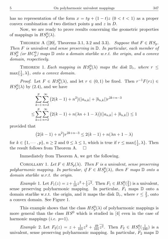
Example 1. Let F1(z) = z+ 110z

2+ 15z

2. Then F1 ∈ HS01(23) is a univalent,

sense preserving polyharmonic mapping. In particular, F1 maps D onto adomain starlike w.r.t. the origin, and it maps the disk Dr, where r ≤ 2

3 , ontoa convex domain. See Figure 1.

This example shows that the class HS0p(λ) of polyharmonic mappings is

more general than the class HS0 which is studied in [4] even in the case ofharmonic mappings (i.e. p=1).

Example 2. Let F2(z) = z + 1101z

2 + 49101z

2. Then F2 ∈ HS01( 1

100) is aunivalent, sense preserving polyharmonic mapping. In particular, F2 maps D


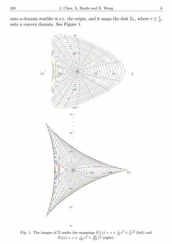
onto a domain starlike w.r.t. the origin, and it maps the disk Dr, where r ≤ 12 ,

onto a convex domain. See Figure 1.

Fig. 1. The images of D under the mappings F1(z) = z + 110z2 + 1

5z2 (left) and

F2(z) = z + 1101

z2 + 49101

z2 (right).


4. EXTREMAL POINTS

First, we determine the distortion bounds for mappings in HSp(λ).

Lemma 1. Suppose that F ∈ HSp(λ). Then, the following statementshold:

(1) For 0 ≤ λ ≤ 12 ,

(1− |b1,1|)|z| −1− |b1,1|2(1 + λ)

|z|2 ≤ |F (z)| ≤ (1 + |b1,1|)|z|+1− |b1,1|2(1 + λ)

|z|2.

Equalities are obtained by the mappings

F (z) = z + |b1,1|eiµz +1− |b1,1|2(1 + λ)

eiνz2,

for properly chosen real µ and ν;

(2) For 12 < λ ≤ 1,

|F (z) ≤ (1 + |b1,1|)|z|+1− |b1,1| − 3(|a1,2|+ |b1,2|)

2(1 + λ)|z|2 + (|a1,2|+ |b1,2|)|z|3

and

|F (z)| ≥ (1− |b1,1|)|z| −1− |b1,1| − 3(|a1,2|+ |b1,2|)

2(1 + λ)|z|2 − (|a1,2|+ |b1,2|)|z|3.

Equalities are obtained by the mappings

F (z) = z+ |b1,1|eiηz+1− |b1,1| − 3(|a1,2|+ |b1,2|)

2(1 + λ)eiϕz2+(|a1,2|+ |b1,2|)eiψz|z|2,

for properly chosen real η, ϕ and ψ.

Proof. Let F ∈ HSp(λ), where λ ∈ [0, 1]. By (2.1), we have

|F (z)| ≤ (1 + |b1,1|)|z|+

(p∑

k=1

∞∑n=2

(|an,k|+ |bn,k|) +

p∑k=2

(|a1,k|+ |b1,k|)

)|z|2.

For 0 ≤ λ ≤ 12 , we have

(4.1) 2(1 + λ) ≤ 2k − 1,

where k ∈ {2, · · · , p}, and

(4.2) 2(1 + λ) ≤ 2(k − 1) + n(λn+ 1− λ),


where k ∈ {1, · · · , p} and n ≥ 2. Then (4.1), (4.2) and (2.4) give

p∑k=1

∞∑n=2

(|an,k|+ |bn,k|) +

p∑k=2

(|a1,k|+ |b1,k|)

≤ 1

2(1 + λ)

(1− |b1,1| −

p∑k=1

∞∑n=2

(2(k − 1) + n(λn+ 1− λ)

−2(1 + λ))(|an,k|+ |bn,k|)−

p∑k=2

((2k − 1)− 2(1 + λ)

)(|a1,k|+ |b1,k|)

),

so

(1− |b1,1|)|z| −1− |b1,1|2(1 + λ)

|z|2 ≤ |F (z)| ≤ (1 + |b1,1|)|z|+1− |b1,1|2(1 + λ)

|z|2.

By (2.1), we obtain

|F (z)| ≤ (1 + |b1,1|)|z|+

(p∑

k=1

∞∑n=2

(|an,k|+ |bn,k|) +

p∑k=3

(|a1,k|+ |b1,k|)

)|z|2

+ (|a1,2|+ |b1,2|)|z|3.

For 12 < λ ≤ 1, we have

(4.3) 2(1 + λ) ≤ 2k − 1,

where k ∈ {3, · · · , p}, and

(4.4) 2(1 + λ) ≤ 2(k − 1) + n(λn+ 1− λ),

where k ∈ {1, · · · , p}, n ≥ 2. Then (4.3), (4.4) and (2.4) imply

p∑k=1

∞∑n=2

(|an,k|+ |bn,k|) +

p∑k=3

(|a1,k|+ |b1,k|)

≤ 1

2(1 + λ)

(1− |b1,1| −

p∑k=1

∞∑n=2

(2(k − 1) + n(λn+ 1− λ)

−2(1 + λ))(|an,k|+ |bn,k|)

−p∑

k=3

(2k − 1− 2(1 + λ)

)(|a1,k|+ |b1,k|)− 3(|a1,2|+ |b1,2|)

).

Then

|F (z)| ≥ (1− |b1,1|)|z| −1− |b1,1| − 3(|a1,2|+ |b1,2|)

2(1 + λ)|z|2 − (|a1,2|+ |b1,2|)|z|3


and

|F (z)| ≤ (1 + |b1,1|)|z|+1− |b1,1| − 3(|a1,2|+ |b1,2|)

2(1 + λ)|z|2 + (|a1,2|+ |b1,2|)|z|3.

The proof of this lemma is complete. �

Remark 1. Suppose that F ∈ HSp(λ) is of the form

F (z) =

p∑k=1

|z|2(k−1)Gk(z) =

p∑k=1

|z|2(k−1)∞∑n=1

(an,kz

n + bn,kzn).

Then for each k ∈ {1, · · · , p},

|Gk(z)| ≤ (|a1,k|+ |b1,k|)|z|+1− |b1,1|2(1 + λ)

|z|2.

Lemma 2. The family HSp(λ) is closed under convex combinations.

Proof. Suppose Fi ∈ HSp(λ) and ti ∈ [0, 1] with∑∞

i=1 ti = 1. Let

Fi(z) =

p∑k=1

|z|2(k−1)∞∑n=1

(a(i)n,kz

n + b(i)n,kz

n).

By Lemma 1, there exists a constant M such that |Fi(z)| ≤ M, for alli = 1, · · · , p. It follows that

∑∞i=1 tiFi(z) is absolutely and uniformly con-

vergent, and by Remark 1, the mapping∑∞

i=1 tiFi(z) is polyharmonic. Since∑∞i=1 tiFi(z) is absolutely and uniformly convergent, we have

∞∑i=1

tiFi(z) =

∞∑i=1

ti

p∑k=1

|z|2(k−1)( ∞∑n=1

a(i)n,kz

n +

∞∑n=1

b(i)n,kz

n

)

=

p∑k=1

|z|2(k−1)( ∞∑n=1

∞∑i=1

tia(i)n,kz

n +

∞∑n=1

∞∑i=1

tib(i)n,kz

n

).

By (2.4), we get

(4.5)

p∑k=1

∞∑n=1

(2(k − 1) + n(λn+ 1− λ)

)(∣∣∣∣∣∞∑i=1

tia(i)n,k

∣∣∣∣∣+

∣∣∣∣∣∞∑i=1

tib(i)n,k

∣∣∣∣∣)

≤∞∑i=1

ti

(p∑

k=1

∞∑n=1

(2(k − 1) + n(λn+ 1− λ)

)(|a(i)n,k|+ |b

(i)n,k|)

)≤ 2.

It follows from

1 ≤p∑

k=1

(2k − 1)

(∣∣∣∣∣∞∑i=1

tia(i)1,k

∣∣∣∣∣+

∣∣∣∣∣∞∑i=1

tib(i)1,k

∣∣∣∣∣)< 2

and (4.5) that∑∞

i=1 tiFi ∈ HSp(λ). �


From Lemma 1, we see that the class HSp(λ) is uniformly bounded, andhence, normal. Lemma 2 implies that HS0

p(λ) is also compact and convex.Then there exists a non-empty set of extremal points in HS0

p(λ).

Theorem 2. The extremal points of HS0p(λ) are the mappings of the

following form:

Fk(z) = z + |z|2(k−1)an,kzn or F ∗k (z) = z + |z|2(k−1)bm,kzm,

where

|an,k| =1

2(k − 1) + n(λn+ 1− λ), for n ≥ 2, k ∈ {1, · · · , p},

and

|bm,k| =1

2(k − 1) +m(λm+ 1− λ), for m ≥ 2, k ∈ {1, · · · , p}.

Proof. Assume that F is an extremal point of HS0p(λ), of the form (2.1).

Suppose that the coefficients of F satisfy the following:p∑

k=1

∞∑n=2

(2(k − 1) + n(λn+ 1− λ)

)(|an,k|+ |bn,k|) < 1.

If all coefficients an,k (n ≥ 2) and bn,k (n ≥ 2) are equal to 0, we let

F1(z) = z +1

2(1 + λ)z2 and F2(z) = z − 1

2(1 + λ)z2.

Then F1 and F2 are in HS0p(λ) and F = 1

2(F1 + F2). This is a contra-diction, showing that there is a coefficient, say an0,k0 or bn0,k0 , of F which isnonzero. Without loss of generality, we may further assume that an0,k0 6= 0.

For γ > 0 small enough, choosing x ∈ C with |x| = 1 properly andreplacing an0,k0 by an0,k0 − γx and an0,k0 + γx, respectively, we obtain twomappings F3 and F4 such that both F3 and F4 are in HS0

p(λ). Obviously,

F = 12(F3+F4). Hence, the coefficients of F must satisfy the following equality:

p∑k=1

∞∑n=2

(2(k − 1) + n(λn+ 1− λ)

)(|an,k|+ |bn,k|) = 1.

Suppose that there exists at least two coefficients, say, aq1,k1 and bq2,k2 oraq1,k1 and aq2,k2 or bq1,k1 and bq2,k2 , which are not equal to 0, where q1, q2 ≥ 2.Without loss of generality, we assume the first case. Choosing γ > 0 smallenough and x ∈ C, y ∈ C with |x| = |y| = 1 properly, leaving all coefficients ofF but aq1,k1 and bq2,k2 unchanged and replacing aq1,k1 , bq2,k2 by

aq1,k1 +γx

2(k1 − 1) + q1(λq1 + 1− λ)and bq2,k2 −

γy

2(k2 − 1) + q2(λq2 + 1− λ),


or

aq1,k1 −γx

2(k1 − 1) + q1(λq1 + 1− λ)and bq2,k2 +

γy

2(k2 − 1) + q2(λq2 + 1− λ),

respectively, we obtain two mappings F5 and F6 such that F5 and F6 are inHS0

p(λ). Obviously, F = 12(F5 + F6). This shows that any extremal point

F ∈ HS0p(λ) must have the form Fk(z) = z + |z|2(k−1)an,kzn or F ∗k (z) =

z + |z|2(k−1)bm,kzm, where

|an,k| =1

2(k − 1) + n(λn+ 1− λ), for n ≥ 2, k ∈ {1, · · · , p},

and

|bm,k| =1

2(k − 1) +m(λm+ 1− λ), for m ≥ 2, k ∈ {1, · · · , p}.

Now, we are ready to prove that for any F ∈ HS0p(λ) with the above

form must be an extremal point of HS0p(λ). It suffices to prove the case of Fk,

since the proof for the case of F ∗k is similar.Suppose there exist two mappings F7 and F8 ∈ HS0

p(λ) such that Fk =tF7 + (1− t)F8 (0 < t < 1). For q = 7, 8, let

Fq(z) =

p∑k=1

|z|2(k−1)∞∑n=1

(a(q)n,kz

n + b(q)n,kz

n).

Then

(4.6) |ta(7)n,k + (1− t)a(8)n,k| = |an,k| =1

2(k − 1) + n(λn+ 1− λ).

Since all coefficients of Fq (q = 7, 8) satisfy, for n ≥ 2 and k ∈ {1, · · · , p},

|a(q)n,k| ≤1

2(k − 1) + n(λn+ 1− λ), |b(q)n,k| ≤

1

2(k − 1) + n(λn+ 1− λ),

(4.6) implies a(7)n,k = a

(8)n,k, and all other coefficients of F7 and F8 are equal to 0.

Thus, Fk=F7=F8, which shows that Fk is an extremal point of HS0p(λ). �

5. CONVOLUTIONS AND NEIGHBORHOODS

Let C0H denote the class of harmonic univalent, convex mappings F of

the form (1.1) with b1 = 0. It is known [11] that the below sharp inequalitieshold:

2|an| ≤ n+ 1, 2|bn| ≤ n− 1.

It follows from ([11], Theorems 5.14) that if H and G are in C0H , then

H ∗ G (or H � G) is sometime not convex, but it may be univalent or even


convex if one of the mappings H and F satisfies some additional conditions.In this section, we consider convolutions of harmonic mappings F ∈ HS0

1(λ)and H ∈ C0

H .

Theorem 3. Suppose that H(z) = z +∑∞

n=2(Anzn + Bnzn) ∈ C0

H andF ∈ HS0

1(λ). Then for 12 ≤ λ ≤ 1, the convolution F ∗ H is univalent and

starlike, and the integral convolution F �H is convex.

Proof. If F (z) = z +∑∞

n=2(anzn + bnzn) ∈ HS0

1(λ), then for F ∗H, weobtain

∞∑n=2

n(|anAn|+ |bnBn|) ≤∞∑n=2

n

(n+ 1

2|an|+

n− 1

2|bn|)

≤∞∑n=2

n(λn+ 1− λ)(|an|+ |bn|) ≤ 1.

Hence, (F ∗H) ∈ HS0. The transformations∫ 1

0

F (z) ∗H(tz)

tdt = (F �H)(z)

now show that (F �H) ∈ HC0. By Theorem A, the result follows. �

Remark 2. The proof of Theorem 3 does not generalize to polyharmonicmappings, when p ≥ 2. For example, let p = 2, and write

H(z) = z +

2∑k=1

|z|2(k−1)∞∑n=2

(An,kzn +Bn,kzn)

and

F (z) = z +

2∑k=1

|z|2(k−1)∞∑n=2

(an,kzn + bn,kzn).

Suppose that |An,k| ≤ n+12 , |Bn,k| ≤ n−1

2 and F ∈ HS02(λ). Then for

λ = 1, the convolution F ∗H is univalent and starlike but it is not clear if thisis true for 1

2 ≤ λ < 1. However, the integral convolution F �H is convex for12 ≤ λ ≤ 1.

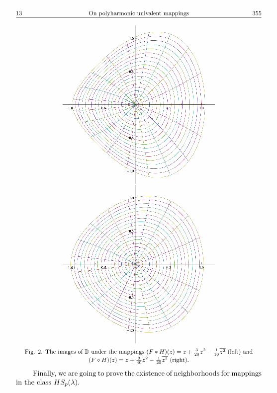
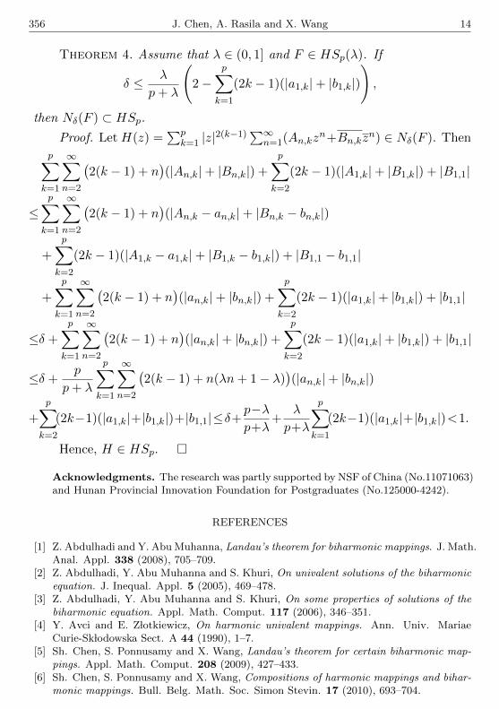
Example 3. Let H(z)=Re{

z1−z}

+ iIm{

z(1−z)2

}∈C0

H . Then H(z) maps Donto the half-plane Re{w} > 1

2 , and let F (z) = z+ 110z

2+ 15z

2 ∈ HS01(23). Then

the convolution F ∗ H is univalent and starlike, and the integral convolutionF �H is convex (see Figure 2).


Fig. 2. The images of D under the mappings (F ∗H)(z) = z + 320z2 − 1

10z2 (left) and

(F �H)(z) = z + 340z2 − 1

20z2 (right).

Finally, we are going to prove the existence of neighborhoods for mappingsin the class HSp(λ).


Theorem 4. Assume that λ ∈ (0, 1] and F ∈ HSp(λ). If

δ ≤ λ

p+ λ

(2−

p∑k=1

(2k − 1)(|a1,k|+ |b1,k|)

),

then Nδ(F ) ⊂ HSp.Proof. Let H(z) =

∑pk=1 |z|

2(k−1)∑∞n=1(An,kz

n+Bn,kzn) ∈ Nδ(F ). Then

p∑k=1

∞∑n=2

(2(k − 1) + n

)(|An,k|+ |Bn,k|) +

p∑k=2

(2k − 1)(|A1,k|+ |B1,k|) + |B1,1|

≤p∑

k=1

∞∑n=2

(2(k − 1) + n

)(|An,k − an,k|+ |Bn,k − bn,k|)

+

p∑k=2

(2k − 1)(|A1,k − a1,k|+ |B1,k − b1,k|) + |B1,1 − b1,1|

+

p∑k=1

∞∑n=2

(2(k − 1) + n

)(|an,k|+ |bn,k|) +

p∑k=2

(2k − 1)(|a1,k|+ |b1,k|) + |b1,1|

≤δ +

p∑k=1

∞∑n=2

(2(k − 1) + n

)(|an,k|+ |bn,k|) +

p∑k=2

(2k − 1)(|a1,k|+ |b1,k|) + |b1,1|

≤δ +p

p+ λ

p∑k=1

∞∑n=2

(2(k − 1) + n(λn+ 1− λ)

)(|an,k|+ |bn,k|)

+

p∑k=2

(2k−1)(|a1,k|+|b1,k|)+|b1,1|≤δ+p−λp+λ

+λ

p+λ

p∑k=1

(2k−1)(|a1,k|+|b1,k|)<1.

Hence, H ∈ HSp. �

Acknowledgments. The research was partly supported by NSF of China (No.11071063)and Hunan Provincial Innovation Foundation for Postgraduates (No.125000-4242).

REFERENCES

[1] Z. Abdulhadi and Y. Abu Muhanna, Landau’s theorem for biharmonic mappings. J. Math.Anal. Appl. 338 (2008), 705–709.

[2] Z. Abdulhadi, Y. Abu Muhanna and S. Khuri, On univalent solutions of the biharmonicequation. J. Inequal. Appl. 5 (2005), 469–478.

[3] Z. Abdulhadi, Y. Abu Muhanna and S. Khuri, On some properties of solutions of thebiharmonic equation. Appl. Math. Comput. 117 (2006), 346–351.

[4] Y. Avci and E. Z lotkiewicz, On harmonic univalent mappings. Ann. Univ. MariaeCurie-Sk lodowska Sect. A 44 (1990), 1–7.

[5] Sh. Chen, S. Ponnusamy and X. Wang, Landau’s theorem for certain biharmonic map-pings. Appl. Math. Comput. 208 (2009), 427–433.

[6] Sh. Chen, S. Ponnusamy and X. Wang, Compositions of harmonic mappings and bihar-monic mappings. Bull. Belg. Math. Soc. Simon Stevin. 17 (2010), 693–704.


[7] Sh. Chen, S. Ponnusamy and X. Wang, Bloch constant and Landau’s theorem for planarp-harmonic mappings. J. Math. Anal. Appl. 373 (2011), 102–110.

[8] J. Chen, A. Rasila and X. Wang, Starlikeness and convexity of polyharmonic mappings.To appear in Bull. Belg. Math. Soc. Simon Stevin, arXiv:1302.2398.

[9] J. Chen, A. Rasila and X. Wang, Landau’s theorem for polyharmonic mappings. Toappear in J. Math. Anal. Appl. arXiv:1303.6760

[10] J. Chen and X. Wang, On certain classes of biharmonic mappings defined by convolution.Abstr. Appl. Anal. 2012, Article ID 379130, 10 pages. doi:10.1155/2012/379130.

[11] J.G. Clunie and T. Sheil-Small, Harmonic univalent functions. Ann. Acad. Sci. Fenn.Math. 9 (1984), 3–25.

[12] P. Duren, Univalent Functions. Spring-Verlag, New York, 1983.[13] P. Duren, Harmonic Mappings in the Plane. Cambridge University Press, Cambridge

2004.[14] M. Fait, J. Krzyz and J. Zygmunt, Explicit quasiconformal extensions for some classes

of univalent functions. Comment. Math. Helv. 51 (1976), 279–285.[15] A.W. Goodman, Univalent functions and nonanalytic curves. Proc. Amer. Math. Soc.

8 (1957), 588–601.[16] J. Happel and H. Brenner, Low Reynolds Number Hydrodynamics with Special Applica-

tions to Particulate Media. Prentice-Hall, Englewood Cliffs, NJ, USA, 1965.[17] D. Kalaj, S. Ponnusamy and M. Vuorinen, Radius of close-to-convexity of harmonic

functions. To appear in Complex Var. Elliptic Equ., 14 pages.doi:10.1080/17476933.2012.759565 arXiv:1107.0610

[18] S.A. Khuri, Biorthogonal series solution of Stokes flow problems in sectorial regions.SIAM J. Appl. Math. 56 (1996), 19–39.

[19] W.E. Langlois, Slow Viscous Flow. Macmillan, New York, NY, USA, 1964.[20] J. Qiao and X. Wang, On p-harmonic univalent mappings (in Chinese). Acta Math.

Sci. 32A (2012), 588–600.[21] C. Pommerenke, Univalent Functions. Vandenhoeck and Ruprecht, Gottingen, 1975.[22] S. Ruscheweyh, Neighborhoods of univalent functions. Proc. Amer. Math. Soc. 18

(1981), 521–528.

Received 13 February 2013 Hunan Normal University,Department of Mathematics,Changsha, Hunan 410081,People’s Republic of China

jiaolongche [email protected]

Hunan Normal University,Department of Mathematics,Changsha, Hunan 410081,People’s Republic of China

andAalto University,

Department of Mathematics and Systems Analysis,P.O. Box 11100, FI-00076 Aalto,

[email protected]

Hunan Normal University,Department of Mathematics,Changsha, Hunan 410081,People’s Republic of China

[email protected]

Documents

On polyharmonic univalent mappings