arX

iv:0

809.

0330

v2 [

hep-

th]

15

Nov

200

8

On orbifolds and free fermion constructions

Ron Donagi Katrin Wendland

November 15, 2008

Abstract

This work develops the correspondence between orbifolds and free fermionmodels. A complete classification is obtained for orbifolds X/G with X theproduct of three elliptic curves and G an abelian extension of a group (Z2)

2

of twists acting on X. Each such quotient X/G is shown to give a geometricinterpretation to an appropriate free fermion model, including the geometricNAHE+ model. However, the semi-realistic NAHE free fermion model isproved to be non-geometric: its Hodge numbers are not reproduced by anyorbifold X/G. In particular cases it is shown that X/G can agree with someBorcea-Voisin threefolds, an orbifold limit of the Schoen threefold, and sev-eral further orbifolds thereof. This yields free fermion models with geometricinterpretations on such special threefolds.

Introduction

This work explores a class of heterotic string theories, more precisely of heteroticconformal field theories, and their geometric interpretations. We consider quan-tum field theories that arise by means of so-called free fermion constructions, andwe study the geometric counterparts of the resulting models. Free fermion modelsare interesting in this context, because mathematically, they are comparativelysimple. They all yield rational conformal field theories, which makes them math-ematically well behaved. On the other hand, there are free fermion models whichcan be interpreted as nonlinear sigma models on tori. In other words, there arespecial points in the moduli space of conformal field theories on tori, where thecorresponding conformal field theories allow a free fermion construction. Hencefor some particular models, there are geometric interpretations at hand, and thenotion of “geometric interpretation” can indeed be made mathematically precise.Finally, more general free fermion models can be included into the discussion byimplementing orbifold techniques.This raises the natural question whether one can find free fermion models whichon the one hand yield semi-realistic string theories, in that they produce exactlythe spectrum of the minimal supersymmetric standard model in the observablemassless sector, and which on the other hand allow a geometric interpretation ona geometric orbifold of a torus. In other words, do any free fermion models exist

1

which connect both to the real world, via the standard model of particle physics,and to geometry, via a mathematically tractable geometric interpretation?Addressing the first part of the task, to our knowledge, [MW86] contains the firsthint that free fermion models could be used to construct semi-realistic models byorbifold-like procedures. These ideas have been further developed by many authors,and models with semi-realistic gauge groups are given e.g. in [FNY90, INQ87],see also [CFN99]. Further references on free fermion models are [KLT87, GO85,ABKW86, ABK87, AB88], and the reader interested in the related topic of covari-ant lattice approaches could consult [FMS86, CFQS86, LLS86, LL87, BFVH87,LLS87, LNS87, LT88, LTZ88].An example of a model of interest to us in this context is the so–called NAHE model[FGKP87, AEHN89, FN93]. It is an example of a semi-realistic heterotic stringtheory, and it can be obtained from a toroidal model by a chain of orbifoldingsof type Z2. In fact, a closer study reveals that a geometric interpretation on anorbifold of a torus, if it exists, must have the form X/G with X the product ofthree elliptic curves and G a semidirect product of a group GS of shifts on X anda subgroup GT ⊂ G which is isomorphic to (Z2)

2, see [Fa93, FFT06].One is hence naturally led to a classification problem: To determine all topo-logically inequivalent Calabi-Yau threefolds that arise by resolving the quotientsingularities in X/G with X the product of three elliptic curves and G a groupof the type described above. This problem is solved in the present paper. A par-tial classification was already given in [DF04], under additional restrictions on the“group of twists” GT . A classification of Calabi-Yau threefolds X/G for which GT

is isomorphic to (Zn)2 with n 6= 2 was given by Jimmy Dillies in [Dil07]. Fromthese classifications one finds a negative answer to the question posed above: Nopurely geometric interpretation of the semi-realistic NAHE free fermion model ex-ists, since for none of the groups G described above, the Hodge numbers h1,1, h2,1

of the resolution of X/G yield three generations h1,1 − h2,1 = 3. In other words,the NAHE and other semi-realistic free fermion models must involve some non-geometric orbifolds.The goal of this paper is to solve the geometric classification problem, to embed itinto the context of free fermion models, and to point out some interesting geometricand model-building features arising from the classification.We start in section 1 with the classification of quotients X/G with G as describedabove. We give a complete list, including the Hodge numbers of the resulting re-solved Calabi-Yau threefolds, as well as their fundamental groups. We also includean (incomplete) discussion of possible coincidences within our list.In section 2 we show that for each of the Calabi-Yau threefolds in our list thereexists a free fermion model whose underlying geometry is X/G. We start witha mathematical review of free fermion constructions. We state and explain therules of the game, and we discuss orbifolds in the free fermion language. Werederive the well-known fact that a particular free fermion model allows a geometricinterpretation on an SO(12) torus. This, along with the discussion of orbifolds,allows us to show that indeed for each model in our list of orbifolds X/G, there isan associated free fermion model.

2

Our list includes a number of Calabi-Yau threefolds that are familiar from othercontexts. The simplest of these is the Vafa-Witten threefold X/(Z2)

2 studied in[VW95]. The NAHE+ model, capturing the geometric part of the NAHE model,is another example. Contrary to popular lore, it is NOT a Z2 orbifold of the Vafa-Witten threefold. We show instead that it can be obtained as a Z2 × Z2 orbifoldof the Vafa-Witten threefold. The full NAHE model is not geometric: we do notobtain any three-generation models in our classification. For other examples, werecover six different types of Borcea-Voisin threefolds [Bor97, Voi93] within ourlist. We also find orbifold limits of Schoen’s threefold [Sch88] and some of itsorbifolds within our list of quotients X/G. This may be of considerable interestbecause precisely these threefolds have been successfully used in the constructionof semi-realistic heterotic string theories in [DOPW02, BD06, BCD06, BD07]. Ifan appropriate degenerate limit of the relevant gauge bundles can be found, thenour result will lead to a dramatic simplification of these heterotic constructions:Free fermion models, after all, are mathematically well understood and technicallyeasy to handle.Discrete torsion may be included in our orbifolds without leaving the realm of freefermion constructions. We note that turning on discrete torsion has a rather mildeffect on the Hodge numbers of our threefolds: we get many of the Hodge numbersof models without torsion, and the only new Hodge pairs are mirrors of existingpairs. Similar observations in more specialized situations have been made before,e.g. in [DW00, PRRV07]. According to Vafa and Witten [VW95], full mirrorsymmetry (as opposed to just the Hodge theoretic matching) is indeed sometimesrealized through discrete torsion. This situation may be specific to (Z2)

2 orbifoldsthough, as suggested in [KS95]. The conclusion of [KS94], suggesting that asym-metric orbifolds should be related to discrete torsion, applies in a different setting,where the emphasis lies on simple current constructions but not on geometric in-terpretations. The NAHE model is not obtainable as a geometric orbifold, with orwithout discrete torsion. Among the six Borcea-Voisin threefolds we obtain, threeare their own mirrors, while the other three are exceptional in the sense that theydo not have mirrors within the Borcea-Voisin construction. Our result that forthese threefolds, there exist associated free fermion models, could therefore well beuseful to shed some light on aspects of mirror symmetry and discrete torsion forthese threefolds.Our basic classification is accomplished with the help of some simple reduction prin-ciples, which reduce the combinatorial complexity and allow us to do everythingby hand. Without these reductions, the amount of calculations required is mas-sive. Indeed, several computer searches have been carried out recently on regionsin the string landscape that overlap ours to various degrees. Nooij [CFN03, Noo06]studied Z2-type free fermion models based on the SO(12) torus. He includes non-geometric orbifolds, and finds a handful of three generation models. A partial listof orbifolds and Hodge numbers is obtained in [PRRV07]. In work in progress,these authors are studying orbifolds with generalized discrete torsion. This appar-ently leads them to recover precisely the complete list of Hodge numbers obtainedhere. The coincidence is quite intriguing; it would be interesting to know whether

3

the objects themselves coincide or whether the Hodge numbers simply fail to cap-ture the relevant data. Note that, for example, the fundamental groups of theirmodels have not been computed. In another work in progress, Kiritisis, Lennekand Schellekens [KLS08] are searching certain free fermion models whose partitionfunctions are left-right symmetric. Due to a language barrier, it is difficult to com-pare their models directly to ours. The list of Hodge numbers they get apparentlyagrees with ours, except that they get one additional model, with Hodge numbers(25,1). The latter is clearly not geometric in our sense: By our assumptions on theorbifolding group G, the G-invariant part of H∗(X,R) contains three dimensionalsubspaces of H1,1(X,R) and of H1,2(X,R), respectively. Hence the Hodge num-bers of all our geometric orbifolds arise by adding contributions of various twistedsectors to the basic (3,3) contribution of the bulk sector, so our Hodge numbersmust be at least 3.

Acknowledgements.

The research leading to this paper has been performed at various locations. The re-search of R.D. has been supported by NSF grants DMS 0139799 and DMS 0612992,and by Research and Training Grant DMS 0636606. K.W. cordially thanks CIRMat Luminy, France and the Penn Math/Physics Group for their hospitality. Herrepeated visits to Philadelphia have been partly funded by Penns NSF FocusedResearch Grant, DMS 0139799, and by her Nuffield Award to Newly AppointedLecturers in Science, Engineering and Mathematics, NAL/00755/G. We have bene-fitted from discussions with A. Bak, V. Bouchard, J. Dillies, A. Faraggi, E. Kiritsis,M. Kreuzer, M. Ratz, and B. Schellekens.

1 A classification of relevant orbifolds

In this section, we discuss a classification of orbifoldings and orbifolds. Restrictingto groups whose so-called twist group GT is isomorphic to (Z2)

2, we introduce anotion of equivalence among such groups, via a reduction principle. Orbifolding theproduct of three elliptic curves by one group yields a quotient which is isomorphicto what is obtained from the product of three different (but isogenous) ellipticcurves by an equivalent group. We give a classification of all such groups up toequivalence. We also calculate some topological data of the resulting orbifolds,namely their Hodge numbers and their fundamental groups. This gives furtherinformation about possible isomorphies among the respective quotients. The mainresults are the tabulation of orbifolds in Section 1.6 and the somewhat incompleteanalysis of coincidences in Section 1.7.

1.1 On a classification of toroidal orbifolds

We work with a 6 (real) dimensional torus X ∼= T 6 with the complex structure ofa product E1 × E2 × E3 of three elliptic curves. Let T0

∼= (Z2)2 ⊂ (Z2)

3 be the

4

Klein group of twists acting on (z1, z2, z3) ∈ X by an even number of sign changes:

t1 : (z1, z2, z3)→ (z1,−z2,−z3),t2 : (z1, z2, z3)→ (−z1, z2,−z3),t3 : (z1, z2, z3)→ (−z1,−z2, z3).

An arbitrary automorphism g of X can be factored uniquely: g = s ◦ gt, where thetwist part gt is an automorphism sending the origin 0 ∈ X to itself, while the shiftpart s is translation by g(0) ∈ X. Any group G of automorphisms fits in an exactsequence

0 −→ GS −→ Gπ−→ G0

T −→ 0,

where GS is the subgroup of shifts contained in G, and G0T is the group of twist

parts of all elements of G, so G0T := {gt|∃ a shift s such that g = s ◦ gt ∈ G}. In

general, G0T is not a subgroup of G. However, it follows from Lemma 1.1.2 below

that we can always reduce to a situation where we can choose a subgroup GT ⊂ Gwhich maps isomorphically onto G0

T under π, and such that G = GS ×GT .Our goal in this section is to study toroidal orbifolds, i.e. quotients X/G, for allfinite groups G whose twist part is T0. We will see that these come in a finitenumber of irreducible families.

Definition 1.1.1 We say that a group G of automorphisms of X is redundant if

it contains a translation by a non zero x ∈ Ei for some i ∈ 1, 2, 3, and is essentialotherwise.

Our first observation (cf.[DF04]) is that there is a simple reduction principle: everytoroidal orbifoldX/G withX = E1×E2×E3 and a given twist partG0

T is also of theformX ′/G′ for some X ′ = E ′

1×E ′2×E ′

3 and some essential group of automorphismsG′ with the same twist part G0

T . Indeed, if the redundant G contains a translationsx by a non zero element x ∈ Ei, then x must be a torsion element, the quotientE ′

i := Ei/x is an elliptic curve, the quotient X ′ := X/x is still a product of threeelliptic curves with one Ei replaced by E ′

i, and

X/G ∼= X ′/G′,

where G′ := G/〈sx〉 fits into an exact sequence

0→ G′S → G′ → G′

T → 0,

with G′S = GS/〈sx〉 and G′

T = G0T as claimed.

We therefore may as well restrict attention to essential groups G.

Lemma 1.1.2 Any essential group G with twist part G0T = T0 is commutative and

isomorphic to the direct product GS ×G0T of its shift and twist parts. All elements

of G are of order 2, and up to conjugation G is contained in Gmax which is the

extension

0→ X[2]→ Gmax → T0 → 0,

where X[2] ∼= (Z2)6 is the group of all points of order 2 in X.

5

Proof: First we show that any g ∈ G has order 2. Let g = s◦ gt ∈ G with s ∈ GS ashift by x ∈ X and gt ∈ G0

T = T0. If gt 6= 1 ∈ G0T then g2 is a shift along x+ gt(x),

i.e. along one of the three elliptic curves, so essence implies g2 = 1. We still needto consider g ∈ GS. The subgroup GS of G is isomorphic to

GS := {x ∈ X|sx ∈ GS} .

The latter is invariant under the action of T0. If it contains x = (x1, x2, x3) it mustalso contain ti(x) hence x + ti(x), which is in Ei. Essence therefore implies that2xi = 0 for all i.It follows that G is commutative and contains a subgroup GT that maps isomor-phically onto the twist group G0

T . Further, it follows that G is isomorphic to thedirect product GS × GT of its shift subgroup GS with any such GT . Now GS is agroup of translations by points of order 2, so it is contained in Gmax. The twistgroup GT need not be contained in Gmax. Its generators can be written in theform:

(z1, z2, z3)→ (x1 + z1, x2 − z2, x3 − z3),(z1, z2, z3)→ (y1 − z1, y2 + z2, y3 − z3)

The order-2 condition requires that x1, y2 and y3−x3 be points of order 2, while thethree remaining variables are unconstrained in the three elliptic curves Ei. Never-theless, one checks immediately that conjugation by an appropriate translation ofX (which also has three complex degrees of freedom, one in each Ei) can be chosento set x2 = x3 = y1 = 0. Such a conjugation takes GT into Gmax and leaves GS

unchanged, completing the proof.

�

In view of the lemma, our essential group G contains a “subgroup of twists” GT

which under π maps isomorphically to G0T , and G is isomorphic to GS × GT . In

the next section we will see that up to conjugation there are four possible actionsof the twist group GT on X.

1.2 Classification of essential automorphism groups

Definition 1.2.1 The rank of an essential automorphism group G is the rank of

GS as a module over Z2.

We will study the possible automorphism groups according to their increasingrank. We will usually describe an automorphism group in terms of a minimal setof generators, listing each generator in the form of a triple (ǫ1δ1, ǫ2δ2, ǫ3δ3), whereǫi ∈ Ei is a point of order 2, and δi ∈ {±} indicates the pure twist part. We takethe period lattice of the elliptic curve Ei to be generated by 2 and 2τ , so the ǫican be one of 0, 1, τ, 1 + τ . The three operations that produce equivalent groupsare change of basis, permutation of the three coordinates zi of the torus, and ashift of one or more of the zi. We start with rank 0, where instead of listing twogenerators we often list all three non zero group elements.

6

Lemma 1.2.2 There are 4 inequivalent groups G = GT of rank 0, given as follows:

(0− 1) : (0+, 0−, 0−), (0−, 0+, 0−), (0−, 0−, 0+),

(0− 2) : (0+, 0−, 0−), (0−, 0+, 1−), (0−, 0−, 1+),

(0− 3) : (0+, 0−, 0−), (0−, 1+, 1−), (0−, 1−, 1+),

(0− 4) : (1+, 0−, 0−), (0−, 1+, 1−), (1−, 1−, 1+).

Remark: In [DF04], only the first of these possibilities, as well as its further quo-tients, were considered, leading to the considerably shorter list there.

Proof: Any rank 0 group is generated by two elements of the form (ǫ1+, ǫ2−, ǫ3−)and (ǫ4−, ǫ5+, ǫ6−). By shifting the three coordinates zi we can clearly arrangethat ǫ2 = ǫ3 = ǫ4 = 0, and by changing the labeling of a homology basis for the Ei

we can take each of the remaining ǫi to be 0 or 1. This leaves us with 8 possibilities,including the four above and

(0+, 0−, 0−), (0−, 1+, 0−), (0−, 1−, 0+);

(1+, 0−, 0−), (0−, 0+, 0−), (1−, 0−, 0+);

(1+, 0−, 0−), (0−, 0+, 1−), (1−, 0−, 1+);

(1+, 0−, 0−), (0−, 1+, 0−), (1−, 1−, 0+).

Of these, the first two are equivalent to (0− 2) under a permutation of the threecoordinates. The third is transformed by a shift of z3 to (1+, 0−, 1−), (0−, 0+, 0−),(1−, 0−, 1+) which is equivalent to (0−3) under a permutation of z1, z2. Similarly,the fourth group is transformed by a shift of z1 to (1+, 0−, 0−), (1−, 1+, 0−),(0−, 1−, 0+) which under a permutation of z2, z3 is equivalent to the third group,hence to (0− 3).One can use similar elementary means to check that the four groups in the state-ment of the lemma are inequivalent. In Section 1.6 we will find the stronger resultthat the corresponding quotients X/G are topologically inequivalent. �

For a group G of higher rank, we list first two generators of G which map ontoa minimal generating set for the twist group GT in the previous (ǫ1δ1, ǫ2δ2, ǫ3δ3)notation; the remaining generators are chosen to be in the shift subgroup GS ⊂ G.Since in this case all the δi are 0, we can omit them, using instead the abbreviatednotation (ǫ1, ǫ2, ǫ3).

Proposition 1.2.3 There are 11 equivalence classes of essential groups in rank 1,14 in rank 2, 6 in rank 3, one in rank 4, and none in higher ranks. They are listed

in the first two columns of Table 1, see Section 1.6.

The proof is elementary and somewhat tedious, using the tools introduced in theproof of Lemma 1.2.2. We leave the details to the reader.

1.3 Orbifold cohomology

Though the techniques are well known, let us briefly summarize for the reader’sconvenience the procedure by which one calculates the Hodge numbers of a minimal

7

resolution of the orbifold X/G. We will assume the situation which is of interestbelow, that isX = E1×E2×E3 equipped with the complex structure of the productof three elliptic curves Ei, and that G is an essential group of the type describedin Section 1.1. In particular, by Lemma 1.1.2, G = GS ×GT with GT

∼= T0 underthe projection π to the twist parts.First observe that the cohomology of X is obtained by taking the wedge prod-uct between the total cohomologies of each elliptic curve Ei. With respect to alocal complex coordinate zi on Ei, the cohomology of the latter is generated by1, dzi, dzi, dzi ∧ dzi. If g ∈ G splits as g = s ◦ ti with ti ∈ T0 into its shift and itstwist part, then g acts on dz1, dz2, dz3 by dzi 7→ dzi and dzj 7→ −dzj for j 6= i,and similarly for the dzk. Hence for the G-invariant part of the cohomology of Xwe find dimensions hp,q

inv, p, q ∈ {0, . . . , 3}, with

(hp,qinv)p,q =

1 0 0 10 3 3 00 3 3 01 0 0 1

.

For example, we have representatives dzi ∧ dzi in H1,1(X) and dz1 ∧ dz2 ∧ dz3 inH2,1(X).Additional contributions to the cohomology of the minimal resolution of X/G comefrom the blow-ups of curves of singularities. Assume that g ∈ G, g 6= 1, has fixedpoints on X. Since by assumption g = s ◦ ti for some ti ∈ T0 and s a shift,this implies that s is a shift by some point x = (x1, x2, x3) ∈ X of order 2 withxi = 0. The fixed locus of g thus consists of 16 copies of Ei. In X/G, the imageyields a curve of singularities of type A1. Its contributions to the cohomology of aresolution of X/〈g〉 have dimensions hp,q

g , p, q ∈ {0, . . . , 3}, with

(hp,q

g

)p,q

=

0 0 0 00 16 16 00 16 16 00 0 0 0

.

The contributions to the cohomology of the resolved quotient X/G are given bythe G-invariant part of these vector spaces. If G has rank r, i.e. G ∼= (Z2)

r+2, thenthe total contribution from blowing up the fixed locus of g = s ◦ ti is

(hp,q

g,inv,A

)p,q

=

0 0 0 00 23−r 23−r 00 23−r 23−r 00 0 0 0

or

(hp,q

g,inv,B

)p,q

=

0 0 0 00 24−r 0 00 0 24−r 00 0 0 0

.

The case hp,qg,inv,B applies if and only if the subgroup of G which maps an irreducible

component of the fixed locus of g in X onto itself is strictly larger than 〈g〉. Indeed,then G contains elements h which map each copy of Ei in the fixed locus of g ontoitself, but which act by multiplication by −1 on dzi and dzi, thus leaving none ofthe cohomology classes counted by h2,1

g and h1,2g invariant, whereas all contributions

to h1,1g and h2,2

g are invariant.

8

1.4 Discrete torsion

In his seminal paper [Vaf86], Cumrun Vafa pointed out that in conformal field the-ory, there is an additional degree of freedom ε ∈ H2(G,U(1)) when orbifolding by agroup G, which is now commonly known as “discrete torsion”. Roughly speaking,one introduces a twisted action of G on the contribution to the cohomology whichcomes from the blow-up of the singular locus in X/G. In the examples that are ofinterest for us, G ∼= (Z2)

r+2. One checks that discrete torsion is compatible withthe reduction principle of Section 1.1, and H2(G,U(1)) = (Z2)

m with m =(

r+22

).

Consider elements g, h ∈ G − {1} such that h 6= g and h maps each componentof the fixed locus of g onto itself. Then the effect of non-trivial discrete torsionε(g, h) amounts to replacing the contributions hp,q

g,inv,B listed above by

(hp,q

g,inv, eB

)

p,q=

0 0 0 00 0 24−r 00 24−r 0 00 0 0 0

.

1.5 Fundamental groups

There is a simple procedure for calculating the fundamental group of an orbifold,which goes back to [DHVW85] in the physics literature. A mathematical versioncan be found in [BH02].

Let a group G act discretely on a simply connected X. Let F be the subgroup ofG generated by all elements which have a fixed point in X. Then the fundamentalgroup of the quotient space X/G is G/F .In our applications, we are interested in the fundamental group of quotients ofthe product X of three elliptic curves, that is X = C3/Λ. We take G to be theextension of the orbifolding group G by the lattice Λ:

0→ Λ→ G→ G→ 0,

so the orbifold is X/G = C3/G. The calculation of the fundamental group of eachof our orbifolds is then a straightforward exercise.

1.6 Tabulation of results

Table 1: The list of automorphism groups

We list the automorphism groups by rank. For each group G we list its twist groupGT , its shift part GS (if non-empty), the Hodge numbers h1,1, h2,1 of a small resolu-tion of X/G, the fundamental group π1(X/G), and the list of contributing sectorsand their contribution. For the fundamental groups we use the abbreviations:

A : the extension of Z2 by Z2 (so H1(X) = (Z2)

3)

B : any extension of (Z2)2 by Z

6 (with various possible H1(X))

C : Z2

D : (Z2)2

9

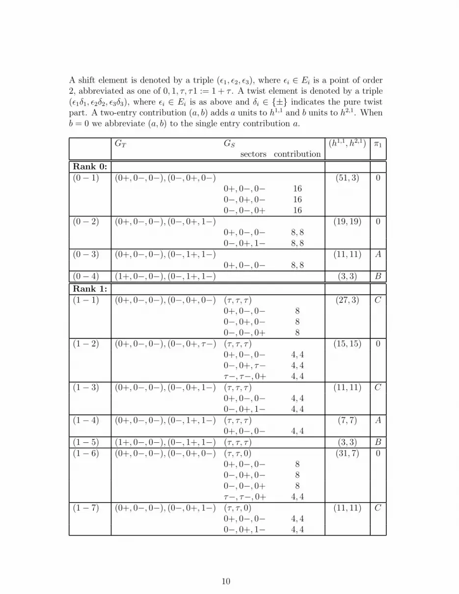
A shift element is denoted by a triple (ǫ1, ǫ2, ǫ3), where ǫi ∈ Ei is a point of order2, abbreviated as one of 0, 1, τ, τ1 := 1 + τ . A twist element is denoted by a triple(ǫ1δ1, ǫ2δ2, ǫ3δ3), where ǫi ∈ Ei is as above and δi ∈ {±} indicates the pure twistpart. A two-entry contribution (a, b) adds a units to h1,1 and b units to h2,1. Whenb = 0 we abbreviate (a, b) to the single entry contribution a.

GT GS (h1,1, h2,1) π1

sectors contribution

Rank 0:

(0− 1) (0+, 0−, 0−), (0−, 0+, 0−) (51, 3) 00+, 0−, 0− 160−, 0+, 0− 160−, 0−, 0+ 16

(0− 2) (0+, 0−, 0−), (0−, 0+, 1−) (19, 19) 00+, 0−, 0− 8, 80−, 0+, 1− 8, 8

(0− 3) (0+, 0−, 0−), (0−, 1+, 1−) (11, 11) A0+, 0−, 0− 8, 8

(0− 4) (1+, 0−, 0−), (0−, 1+, 1−) (3, 3) B

Rank 1:

(1− 1) (0+, 0−, 0−), (0−, 0+, 0−) (τ, τ, τ) (27, 3) C0+, 0−, 0− 80−, 0+, 0− 80−, 0−, 0+ 8

(1− 2) (0+, 0−, 0−), (0−, 0+, τ−) (τ, τ, τ) (15, 15) 00+, 0−, 0− 4, 40−, 0+, τ− 4, 4τ−, τ−, 0+ 4, 4

(1− 3) (0+, 0−, 0−), (0−, 0+, 1−) (τ, τ, τ) (11, 11) C0+, 0−, 0− 4, 40−, 0+, 1− 4, 4

(1− 4) (0+, 0−, 0−), (0−, 1+, 1−) (τ, τ, τ) (7, 7) A0+, 0−, 0− 4, 4

(1− 5) (1+, 0−, 0−), (0−, 1+, 1−) (τ, τ, τ) (3, 3) B(1− 6) (0+, 0−, 0−), (0−, 0+, 0−) (τ, τ, 0) (31, 7) 0

0+, 0−, 0− 80−, 0+, 0− 80−, 0−, 0+ 8τ−, τ−, 0+ 4, 4

(1− 7) (0+, 0−, 0−), (0−, 0+, 1−) (τ, τ, 0) (11, 11) C0+, 0−, 0− 4, 40−, 0+, 1− 4, 4

10

GT GS (h1,1, h2,1) π1

sectors contribution

(1− 8) (0+, 0−, 0−), (0−, 1+, 0−) (τ, τ, 0) (15, 15) 00+, 0−, 0− 4, 40−, 1−, 0+ 4, 4τ−, τ1−, 0+ 4, 4

(1− 9) (0+, 0−, 0−), (0−, 1+, 1−) (τ, τ, 0) (7, 7) A0+, 0−, 0− 4, 4

(1− 10) (1+, 0−, 0−), (0−, 1+, 0−) (τ, τ, 0) (11, 11) A1−, 1−, 0+ 4, 4τ1−, τ1−, 0+ 4, 4

(1− 11) (1+, 0−, 0−), (0−, 1+, 1−) (τ, τ, 0) (3, 3) B

Rank 2:

(2− 1) (0+, 0−, 0−), (0−, 0+, 0−) (1, 1, 1), (τ, τ, τ) (15, 3) D0+, 0−, 0− 40−, 0+, 0− 40−, 0−, 0+ 4

(2− 2) (0+, 0−, 0−), (0−, 0+, 1−) (1, 1, 1), (τ, τ, τ) (9, 9) C0+, 0−, 0− 2, 20−, 0+, 1− 2, 21−, 1−, 0+ 2, 2

(2− 3) (0+, 0−, 0−), (0−, 0+, 0−) (1, 1, 1), (τ, τ, 0) (17, 5) C0+, 0−, 0− 40−, 0+, 0− 40−, 0−, 0+ 4τ−, τ−, 0+ 2, 2

(2− 4) (0+, 0−, 0−), (0−, 0+, 1−) (1, 1, 1), (τ, τ, 0) (11, 11) 00+, 0−, 0− 2, 20−, 0+, 1− 2, 21−, 1−, 0+ 2, 2τ1−, τ1−, 0+ 2, 2

(2− 5) (0+, 0−, 0−), (0−, 0+, τ−) (1, 1, 1), (τ, τ, 0) (7, 7) D0+, 0−, 0− 2, 20−, 0+, τ− 2, 2

(2− 6) (0+, 0−, 0−), (0−, 0+, 0−) (1, 1, 1), (τ, 1, 0) (19, 7) 00+, 0−, 0− 40−, 0+, 0− 40−, 0−, 0+ 4τ1−, 0+, 1− 2, 2τ−, 1−, 0+ 2, 2

(2− 7) (0+, 0−, 0−), (0−, 0+, τ−) (1, 1, 1), (τ, 1, 0) (9, 9) C0+, 0−, 0− 2, 20−, 0+, τ− 2, 2τ1−, 0+, τ1− 2, 2

11

GT GS (h1,1, h2,1) π1

sectors contribution

(2− 8) (0+, 0−, 0−), (0−, τ+, τ−) (1, 1, 1), (τ, 1, 0) (5, 5) A0+, 0−, 0− 2, 2

(2− 9) (0+, 0−, 0−), (0−, 0+, 0−) (0, 1, 1), (1, 0, 1) (27, 3) 00+, 0−, 0− 40−, 0+, 0− 40−, 0−, 0+ 40+, 1−, 1− 41−, 0+, 1− 41−, 1−, 0+ 4

(2− 10) (0+, 0−, 0−), (0−, 0+, τ−) (0, 1, 1), (1, 0, 1) (11, 11) 00+, 0−, 0− 2, 20+, 1−, 1− 2, 20−, 0+, τ− 2, 2

1−, 0+, τ1− 2, 2(2− 11) (0+, 0−, 0−), (0−, τ+, τ−) (0, 1, 1), (1, 0, 1) (7, 7) A

0+, 0−, 0− 2, 20+, 1−, 1− 2, 2

(2− 12) (τ+, 0−, 0−), (0−, τ+, τ−) (0, 1, 1), (1, 0, 1) (3, 3) B(2− 13) (0+, 0−, 0−), (0−, 0+, 0−) (1, 1, 0), (τ, τ, 0) (21, 9) 0

0+, 0−, 0− 40−, 0+, 0− 40−, 0−, 0+ 41−, 1−, 0+ 2, 2τ−, τ−, 0+ 2, 2

τ1−, τ1−, 0+ 2, 2(2− 14) (0+, 0−, 0−), (0−, 0+, 1−) (1, 1, 0), (τ, τ, 0) (7, 7) D

0+, 0−, 0− 2, 20−, 0+, 1− 2, 2

Rank 3:

(3− 1) (0+, 0−, 0−), (0−, 0+, 0−) (0, τ, 1), (12, 6) 0(τ, 1, 0), (1, 0, τ)

0+, 0−, 0− 20−, 0+, 0− 20−, 0−, 0+ 20+, τ−, 1− 1, 11−, 0+, τ− 1, 1τ−, 1−, 0+ 1, 1

12

GT GS (h1,1, h2,1) π1

sectors contribution

(3− 2) (0+, 0−, 0−), (0−, 0+, 1−) (0, τ, 1), (12, 6) 0(τ, 1, 0), (1, 0, τ)

0+, 0−, 0− 1, 10−, 0+, 1− 20−, τ−, 0+ 20+, τ−, 1− 2

1−, 0+, τ1− 1, 1τ−, τ1−, 0+ 1, 1

(3− 3) (0+, 0−, 0−), (0−, 0+, 0−) (1, 1, 0), (17, 5) 0(τ, τ, 0), (1, τ, 1)

0+, 0−, 0− 20−, 0+, 0− 20−, 0−, 0+ 2

0+, τ1−, 1− 2τ1−, 0+, 1− 21−, 1−, 0+ 1, 1τ−, τ−, 0+ 1, 1

τ1−, τ1−, 0+ 2(3− 4) (0+, 0−, 0−), (0−, 0+, τ−) (1, 1, 0), (7, 7) C

(τ, τ, 0), (1, τ, 1)0+, 0−, 0− 1, 10−, 0+, τ− 1, 1

0+, τ1−, 1− 1, 1τ1−, 0+, τ1− 1, 1

(3− 5) (0+, 0−, 0−), (0−, 0+, 0−) (0, 1, 1), (15, 3) C(1, 0, 1), (τ, τ, τ)

0+, 0−, 0− 20−, 0+, 0− 20−, 0−, 0+ 20+, 1−, 1− 21−, 0+, 1− 21−, 1−, 0+ 2

(3− 6) (0+, 0−, 0−), (0−, 0+, τ−) (0, 1, 1), (9, 9) 0(1, 0, 1), (τ, τ, τ)

0+, 0−, 0− 1, 10−, 0+, τ− 1, 1τ−, τ−, 0+ 1, 10+, 1−, 1− 1, 1

1−, 0+, τ1− 1, 1τ1−, τ1−, 0+ 1, 1

13

GT GS (h1,1, h2,1) π1

sectors contribution

Rank 4:

(4− 1) (0+, 0−, 0−), (0−, 0+, 0−) (0, τ, 1), (τ, 1, 0), (15, 3) 0(1, 0, τ), (1, 1, 1)

0+, 0−, 0− 10+, τ−, 1− 1

0+, 1−, τ1− 10+, τ1−, τ− 10−, 0+, 0− 11−, 0+, τ− 1τ1−, 0+, 1− 1τ−, 0+, τ1− 10−, 0−, 0+ 1τ−, 1−, 0+ 1

1−, τ1−, 0+ 1τ1−, τ−, 0+ 1

As follows from the discussion in Section 1.4, for some of the orbifolds listed abovethere may be a non-trivial effect on the resulting Hodge numbers, when twistedactions of G are allowed on the blow-ups of curves of singularities in X/G, that iswhen discrete torsion is taken into account. The most popular example of this typeis our model (0− 1) which was extensively studied in [VW95]. In that paper, theauthors discover that turning on nontrivial discrete torsion ε ∈ Z2 in this exampleof an orbifold by G ∼= (Z2)

2 produces its mirror partner. From our discussion it isindeed not hard to check that the effect of ε = −1 instead of ε = 1 is a swap ofthe Hodge numbers h1,1, h2,1.In general, for each model in our list, an interchange of h1,1 and h2,1 can be achievedby choosing a certain value for discrete torsion. Other types of discrete torsionexist for some of the models, typically producing Hodge number pairs that areintermediate between those of the original orbifold and its mirror. All Hodge pairsobtained this way arise also from other orbifolds without discrete torsion, so theycan also be found elsewhere in our table. we list the possible Hodge numbers below:

model possible values of (h1,1, h2,1)

(2− 9) (27, 3), (15, 15), (3, 27)(3− 3) (17, 5), (11, 11), (5, 17)(3− 5) (15, 3), (9, 9), (3, 15)(4− 1) (15, 3), (12, 6), (9, 9), (6, 12), (3, 15)

Thus we find that the main effect of discrete torsion on our list of possible Hodgenumbers (h1,1, h2,1) is a symmetrization with respect to h1,1 ↔ h2,1. We thereforerefrain from a further study of the resulting geometries. In particular, we do notexamine whether there are any Calabi-Yau threefolds obtained from allowing non-trivial discrete torsion which agree with any of the models listed in Table 1, ortheir mirrors.

14

Table 2: The orbifold family tree

Below we list all those orbifoldings which are realized as free quotients betweenorbifolds listed in Table 1. In the diagrams, each entry is of the form

((r−n)

(h1,1,h2,1)

),

where (r−n) is the label in Table 1, and (h1,1, h2,1) gives the corresponding Hodgenumbers.We first list all free quotients relating orbifolds X/G with fundamental group oftype A: (

(1−4)(7,7)

)−→

((2−8)(5,5)

)

ր ր((0,3)

(11,11)

)−→

((1−9)(7,7)

)

ց ց((1−10)(11,11)

)−→

((2−11)(7,7)

)

Next we list all free quotients relating orbifolds X/G with fundamental group oftype B: (

(0,4)(3,3)

)−→

((1−5)(3,3)

)

ց ((1−11)(3,3)

)−→

((2−12)(3,3)

)

We list the remaining quotients, where the three columns give orbifolds with fun-damental group 0, C, D, respectively:

15

((0−1)(51,3)

)−→

((1−1)(27,3)

)−→

((2−1)(15,3)

)

((0,2)

(19,19)

)−→

((1−3)(11,11)

)−→

((2−5)(7,7)

)

ց ր((1−7)(11,11)

)−→

((2−14)(7,7)

)

((1−2)(15,15)

)−→

((2−2)(9,9)

)

((1−6)(31,7)

)−→

((2−3)(17,5)

)

((1−8)(15,15)

)−→

((2−7)(9,9)

)

((2−4)(11,11)

)

((2−6)(19,7)

)

((2−9)(27,3)

)−→

((3−5)(15,3)

)

((2−10)(11,11)

)−→

((3−4)(7,7)

)

((2−13)(21,9)

)

((3−1)(12,6)

)

((3−2)(12,6)

)

((3−3)(17,5)

)

((3−6)(9,9)

)

((4−1)(15,3)

)

1.7 On coincidences in the list

The Hodge numbers and fundamental group data in Table 1 do not suffice tocompletely distinguish the orbifolds on our list. We can obtain some additionaltopological information:

Lemma 1.7.1 The four orbifolds whose fundamental group is an extension of

(Z2)2 by Z6 (“type B”), labeled (0− 4), (1− 5), (1− 11), (2− 12), all with Hodge

numbers (3, 3), are topologically inequivalent: their fundamental groups are not

isomorphic.

Proof: Each of these four orbifolds Xi is a quotient of C3 by a group Gi actingwithout fixed points, so Fi = {1}, Gi = Gi/Fi = π1(Xi).Each Gi is generated by the two twists (1+, 0−, 0−), (0−, 1+, 1−), plus a rank 6lattice Li of translations, with respective generators:

(0− 4) : (2, 0, 0), (0, 2, 0), (0, 0, 2), (2τ, 0, 0), (0, 2τ, 0), (0, 0, 2τ);

(1− 5) : (2, 0, 0), (0, 2, 0), (0, 0, 2), (2τ, 0, 0), (0, 2τ, 0), (τ, τ, τ);

16

(1− 11) : (2, 0, 0), (0, 2, 0), (0, 0, 2), (2τ, 0, 0), (τ, τ, 0), (0, 0, 2τ);

(2− 12) : (2, 0, 0), (0, 2, 0), (0, 0, 2), (2τ, 0, 0), (0, τ, τ), (τ, 0, τ).

The commutator [G,G] is generated by:

[(1+, 0−, 0−), (0−, 1+, 1−)] = (2,−2, 2);

[(1+, 0−, 0−), Li] = {(0,−2b,−2c)|(a, b, c) ∈ Li} ;

[(0−, 1+, 1−), Li] = {(−2a, 0,−2c)|(a, b, c) ∈ Li} .Consider the four quotients H1 = G/[G,G] for G = Gi. The images of the twotwists square to the non zero elements (2, 0, 0) and (0, 2, 0) respectively, which inall four cases are distinct in H1. These twists therefore generate a subgroup (Z4)

2

of H1 which contains the image of the (Z2)2 orbit of the Z3 of 1-cycles. Therefore,

each of the quotients H1 = G/[G,G] is a product H1×Hτ where H1 = (Z4)2 comes

from the twists and the three 1-cycles, while Hτ comes from the three τ -cycles.Explicitly, the four groups Hτ are: (Z2)

3,Z4, (Z2)2, (Z2)

2, so the four quotientsH1 = G/[G,G] are:

(0− 4) : (Z4)2 × (Z2)

3,

(1− 5) : (Z4)3,

(1− 11) : (Z4)2 × (Z2)

2,

(2− 12) : (Z4)2 × (Z2)

2.

It remains to distinguish between the last two orbifolds. For that, note that inthese cases the extension 0 → Li → Gi → (Z2)

2 → 0 is uniquely determined byLi. In fact, the projection Gi → (Z2)

2 is just the composition of the abelian-ization G → G/[G,G] with multiplication by 2 in the abelian group G/[G,G].So any isomorphism of the two groups Gi induces an isomorphism of the exten-sions, hence of the actions of (Z2)

2 on Li. This action sends (a, b, c) ∈ Li to(a,−b,−c), (−a, b,−c), (−a,−b, c) respectively. The sum of the three sublatticesfixed under these three involutions is the lattice L(0−4), which has index 2 in Li

for i = (1 − 11) and index 4 for i = (2 − 12), completing the proof that the fourfundamental groups are pairwise non-isomorphic. �

Unfortunately, comparable topological information is harder to get for fundamen-tal groups of the other types. For example, one can check that the extension of Z2

by Z2, of “type A”, is unique, with homology group H1(X) = (Z2)3. This leaves

us with the following undistinguished cases:

(h1,1, h2,1) π1 cases

(15, 15) 0 (1− 2), (1− 8)(11, 11) 0 (2− 4), (2− 10)(12, 6) 0 (3− 1), (3− 2)(11, 11) A (0− 3), (1− 10)(7, 7) A (1− 4), (1− 9), (2− 11)

(11, 11) C (1− 3), (1− 7)(9, 9) C (2− 2), (2− 7)(7, 7) D (2− 5), (2− 14)

17

For some of these cases we are able to give a definite answer whether or not thecorresponding threefolds agree. Specifically, the models (0 − 3) and (1 − 10) areof same topological type, although their complex structure is different, as we shallsee in Section 3.2. Together with the orbifold family tree of Table 2 this suggeststhat the three models (1−4), (1−9), and (2−11) may be topologically equivalentas well. We know that the models (1 − 3) and (1 − 7) are distinct as families ofcomplex varieties, and so are (2 − 5) and (2 − 14), as we shall see in Section 3.3.It is not clear to us whether they are topologically equivalent.

2 Free fermion models

In this section, we briefly review free fermion models, giving the basic structure ofthose conformal field theories which are obtained from free fermion constructions.Moreover, we explain how the particular geometric orbifolds that we have classifiedin Section 1 are related to these models.

2.1 Model building with free fermions

We use free fermion models to construct heterotic string theories in D = 4 dimen-sions. As the name suggests, the basic ingredients to free fermion models are therepresentations of the free fermion algebra, see Appendix B. Let H0, H1 denotethe irreducible Fock space representations of the free fermion algebra in the NSand the R sector, respectively, enlarged by (−1)F with F the worldsheet fermionnumber operator. Roughly, a free fermion model is obtained from an appropriatetensor product of Fock spaces H0, H1 by a certain projection, whose properties arepartly governed by the consistency conditions of string theory.In a heterotic theory the left handed side carries at least N = 1 supersymmetry,whereas the right handed side is not supersymmetric. We fermionize all internaldegrees of freedom, thus allowing a description in terms of free fermions. Exter-nal bosons are not fermionized, since they are free uncompactified fields, wherefermionization does not apply to add degrees of freedom. The various anomalycancellation conditions then dictate the following structure: In the left handedsector, we have four external bosons and fermions, two of which are transver-sal in the light cone gauge, ∂Xµ, ψ

µ, µ ∈ {0, 1}. Since the superstring criti-cal dimension is 10, where each coordinate direction corresponds to three freefermions, there are (10 − 4) · 3 = 18 internal fermions χi, yi, wi, i ∈ {1, . . . , 6}.The left handed worldsheet supercurrent, which generates the local conformaltransformations, is then given in light cone gauge by:

∑µ :ψµ∂Xµ: +

∑i :χiyiwi:

[ABKW86, GO85, GNO85, GKO86, DKPR85]. On the right handed side we havefour external bosons, two of which are transversal, ∂Xµ, µ ∈ {0, 1}. Further-more, given the bosonic critical dimension 26 with each coordinate direction cor-responding to two free fermions, there are (26 − 4) · 2 = 44 internal fermions

Φi, i ∈ {1, . . . , 44}. All in all, including external fermions, we have 20 + 44 = 64

fermionic degrees of freedom, and we introduce indices j ∈ {1, . . . , 64} for them in

18

the order ψ0, ψ1, χ1, . . . , χ6, y1, . . . , y6, w1, . . . , w6, Φ1, . . . , Φ

44.

To construct a full theory we need to specify which combinations of spin structuresfor each of the 64 real free fermions contribute. Since many of our free fermionsresult from bosonization, the respective spin structures are coupled pairwise. Thisis also always true for ψ0, ψ1, to ensure consistency of the coupling with worldsheetgravitinos. If the yj, wj combine to six left handed bosons with currents i :yjwj:,then each pair yj, wj must have coupled spin structures. This is the case for freefermion models with geometric interpretation on a real six-torus, but not in gen-eral, so we will not assume such couplings in general. However, if our free fermionmodel arises from a heterotic compactification on a Calabi-Yau manifold with gauge

group in E8×E8, then among the right handed Φithere must be six pairs yielding

the antiholomorphic partners of the yi, wi, which we then denote yi, wi instead of

Φ1, . . . ,Φ

12. Then yi +yi and wi +wi are the fields corresponding to the respective

fermionized coordinates, so yi, yi and wi, wi are pairs with coupled spin structures.

The remaining 32 right handed Φisplit into two sets ϕi, φ

iof eight complex Dirac

fermions each, to allow bosonization to 8 independent currents for each E8 sum-mand of the gauge Kac-Moody algebra, cf. [ABKW86, GO85, GNO85, GKO86].Each Dirac fermion is equivalent to one boson, so the notation implies that the

real and imaginary parts of ϕi, φialso have coupled spin structures. Finally, the

heterotic theory on a Calabi-Yau manifold has (N,N) = (2, 0) worldsheet super-symmetry with U(1) current given by, say,

∑i :χ2j−1χ2j:, which is reflected in a

pairwise coupling of spin structures for the χi, here (χ1, χ2), (χ3, χ4), (χ5, χ6).For what follows we therefore assume that the 64 fermions are arranged into pairswith coupled spin structures. In other words, we fix an injective vectorspace ho-momorphism ι : F

322 −→ F

642 and a fixpoint free involution σ on {1, . . . , 64} such

that for all α ∈ im(ι) and all i ∈ {1, . . . , 64} we have αi = ασ(i). For α ∈ im(ι) wethen define

Hα := pr

(64⊗

i=1

Hiαi

),

where∗ pr acts trivially on all Hi0 but projects Hj

1⊗Hσ(j)1 onto a chosen irreducible

representation of the algebra generated by the ψja, ψ

σ(j)a with a ∈ Z and the total

worldsheet fermion number operator (−1)Fj+Fσ(j) (see Appendix B).While a single fermion can live in one of two sectors (NS or R), states in our fulltheory fall into sectors Hα characterized by α ∈ im(ι) ⊂ F64

2 . By the above, therelevant contributions to the partition function have the form

Z

[αβ

](τ, τ) :=

∏20j=1Z

[αj

βj

](τ)∏64

j=21 Z

[αj

βj

](τ )

(B.2)= trHα

[∏j(−1)βjFjqL0−c/24 qL0−c/24

],

(2.1)

where L0 =∑20

j=1Lj0, L0 =

∑64j=21L

j

0 are the total left and right handed Virasorozero modes and c = 10, c = 22 the total central charges. In the following we also

∗Here and in the following, indices j serve as a reminder that we are considering the jth freefermion, j ∈ {1, . . . , 64}.

19

abbreviate ∏

j

(−1)βjFj = eπiβ·F .

As mentioned above, our models include two left-handed external fermions, ψµ, µ ∈{0, 1}, and consistency of their coupling to worldsheet gravitinos translates intothe requirement that these two must always have the same spin structures. Thismeans that we can assign a definite spin statistic δα ∈ {±1} to each sector Hα

which contributes to our theory:

∀α ∈ F642 with α1 = α2: δα := (−1)α1 ,

where α ∈ im(ι) implies α1 = α2. By definition, sectors Hα with positive spinstatistic δα = 1 contain the spacetime bosons, whereas sectors Hα with nega-tive spin statistic δα = −1 contain the spacetime fermions. We can thus use thespacetime fermion number operator FS, where (−1)FS acts trivially on spacetimebosons and by multiplication with (−1) on spacetime fermions. We can now makean ansatz for the Hilbert space H and the partition function

Z(τ, τ) = trH

[(−1)FSqL0−c/24 qL0−c/24

](2.2)

of the total fermionized theory. Namely, we begin by requiring that Z has the form

Z(τ, τ) = 1|F|

∑

α,β∈FC

[αβ

]Z

[αβ

](τ, τ), C

[αβ

]∈ Z, (2.3)

for some F ⊂ F642 such that for every α ∈ F there is a β ∈ F with C

[αβ

]6= 0. Note

that if Z is obtained from some pre-Hilbert space H by (2.2), then Z vanishes iff inH there is a 1: 1 correspondence between spacetime bosons and spacetime fermionswhich respects the (L0, L0) eigenvalues. In other words, Z(τ, τ) ≡ 0 iff our theorypossesses spacetime supersymmetry, see also Section 2.3.Let us now give a description of H which yields (2.2) with (2.3), and let us discuss

appropriate restrictions on the coefficients C

[αβ

]. First rewrite (2.3) with (2.1) to

find

Z(τ, τ) =∑

α∈FδαZα(τ, τ ), Zα(τ, τ) = trHα

[PFqL0−c/24 qL0−c/24

],

PF :⊕

α∈F Hα −→⊕

α∈F Hα, PF|Hα

:= 1|F|∑

β∈F δαC

[αβ

]· eπiβ·F ,

(2.4)where by construction (−1)FS

|Hα= δα. Then (2.2) holds with H = PF ⊕α∈F Hα.

We wish to interpret PF as a projection operator. To ensure that PF ◦ PF = PF

one checks that it suffices to assume that F ⊂ F642 is a vector space and that

∀α, β, γ ∈ F : C

[α

β + γ

]= δα C

[αβ

]C

[αγ

].

20

In other words,

∀α ∈ F : χα : F −→ {±1}, χα(β) := δαδβC

[αβ

]

is a character. For later convenience we introduce the notation

χ : F × F −→ {±1}, χ

[αβ

]:= δαδβC

[αβ

]

and indeed assume for the following that F is a vector space and that

∀α, β, γ ∈ F : χ

[α

β + γ

]= χ

[αβ

]χ

[αγ

]∈ {±1}. (2.5)

Then the remaining restrictions on the possible choices of χ

[αβ

]will come from the

fact that the partition function Z must be modular invariant and that all fields inH = PF ⊕

α∈FHα must be pairwise semi-local. We introduce

∀α, β ∈ im(ι): α · β :=1

2

20∑

j=1

αjβj −1

2

64∑

j=21

αjβj = αL · βL − αR · βR,

α2 := α · α(2.6)

with αL, βL ∈ F202 , αR, βR ∈ F44

2 . This induces a scalar product on F322∼= im(ι)

with signature (n+, n−, n0). The form (2.6) encodes the conformal dimensions ofthe ground states in Hα for α ∈ F if we lift F ⊂ F64

2 to Z64 with entries in{0, 1}. Namely, since NS ground states in our Fock space representation of the freefermion algebra have vanishing conformal dimension, whereas the R ground statesof a single free fermion have dimension 1

16, we see that the ground states of Hα

have conformal dimensions

(h, h) =(αL · αL

8,αR · αR

8

). (2.7)

To get a well-defined fermionic theory, namely to ensure semi-locality, all conformalspins have to be half integer, h− h ∈ 1

2Z. Since on Hα, the condition h− h ∈ 1

2Z

depends solely on the conformal spin of the ground state as obtained from (2.7),we thus need

∀α ∈ F : α2 ≡ 0(4). (2.8)

Vice versa, if this constraint holds, then one checks that on H a so-called OPE canbe introduced consistently, as is necessary to construct a CFT.Every theory must contain a vacuum sector H0, as follows from 0 ∈ F , and unique-

ness of the vacuum dictates C

[00

]= 1. By the transformation properties listed in

Appendix A, the modular transformation τ 7→ − 1τ+1

maps Z

[00

]to Z

[10

]. Since Z

21

must be modular invariant, this implies that 0 ∈ F entails 1 ∈ F , the vector withall 64 entries given by 1. Hence by (2.8) we need n+−n− ≡ 0(4). In fact, assuming(2.5), modular invariance of the partition function holds if we also impose

C

[αβ

]= C

[βα

], C

[α

α+ 1

]= −δα e−πiα2/4. (2.9)

The latter condition is only consistent if n+ − n− ≡ 4(8). These rules now allow

us to restrict attention to C

[bibj

]with bi, bj ∈ B a basis of F . For example,

B0 = {1},BSUSY = {1, s} with si =

{1 if i ≤ 8,0 otherwise,

Btor = {1, s, ξ1, ξ2} with (ξ1)i =

{1 if i > 48,0 otherwise,

(ξ2)i =

{1 if 32 < i ≤ 48,0 otherwise.

(2.10)

Consistent choices for the values of C are obtained, e.g., as follows:

β 0 1 s ξ1 ξ2α

0 1 −1 −1 1 1

1 −1 −1 −1 (−1)ε1 (−1)ε2

s −1 −1 −1 (−1)ε′1 (−1)ε′2

ξ1 1 (−1)ε1 (−1)ε′1 (−1)ε1 (−1)κ

ξ2 1 (−1)ε2 (−1)ε′2 (−1)κ (−1)ε2

εi, ε′i, κ ∈ {0, 1}.

2.2 GSO and orbifold projections

In general, from the partition function (2.2) of a CFT we can read the net numberof (spacetime) bosonic minus fermionic states in H which are eigenvectors of theVirasoro zero modes L0, L0 with any pair of eigenvalues h, h ∈ R. The specialstructure of the partition function (2.4) allows us to determine the numbers ofbosonic and fermionic contributions separately by hand. Namely, for each β ∈ F ,(2.9) implies

∀α, γ ∈ F : C

[αγ

]Z

[αγ

]+ C

[α

γ + β

]Z

[α

γ + β

]

= C

[αγ

](Z

[αγ

]+ δαC

[αβ

]Z

[α

γ + β

]).

(2.11)

22

Since Z

[αγ

]and Z

[α

γ + β

]differ by an insertion of (−1)Fj in the trace trHα

in

each component j where βj = 1, this amounts to projecting onto states |σ〉α ∈ Hα

which obey

δα C

[αβ

]eπiβ·F |σ〉α = |σ〉α. (2.12)

The condition (2.12) is often called GSO-projection. Since (2.9) also implies that

∀α ∈ F : C

[α0

]= δα,

so that (2.12) trivially holds for β = 0, and since F is a vector space over F2, wesee that |σ〉α remains in the spectrum of our theory iff (2.12) holds for all basiselements β = bj ∈ B.The interpretation of PF as projection operator allows us to relate different choicesof bases B, B′ by orbifolding. Namely, if B ⊂ B′ with r = |B| and r′ = |B′|, thenthe corresponding theories are related by orbifolding with respect to a group G of

type (Z2)r′−r, as long as the coefficients C

[αβ

]for α, β ∈ span

F2B agree. To see

this, let

B = {b1, . . . , br} and B′ = {b1, . . . , br, br+1, . . . , br′} = B ∪ B⊥.

DefineF := span

F2B, F ′ := span

F2B′, F⊥ := span

F2B⊥.

Recall that the CFTs C, C′ corresponding to the bases B and B′, respectively, haveunderlying pre-Hilbert spaces

H = PF⊕

α∈FHα, H′ = PF ′

⊕

α′∈F ′

Hα′ .

We now wish to reinterpret H′ as arising from H by orbifolding, i.e. by rewriting

H′ = HG ⊕(Htwist

)G,

where a superscript G denotes the G-invariant subspace of a given vectorspace, andHtwist :=

⊕γ 6=0Hγ is the sum of the twisted sectors. We will see that this amounts

to a simple reordering of the summands of H′. Indeed, the sectors Hα′ , α′ ∈ F ′,which contribute to the theory C′ associated to B′ can be listed as follows:

∀ γ ∈ F⊥ : Horbγ :=

⊕

eα∈FH

eα+γ, so H′ = PF ′⊕

γ∈F⊥

Horbγ .

Using PF ′

= PF⊥ ◦ PF and for all γ ∈ F⊥: Horbγ := PFHorb

γ , we observe H′ =

PF⊥⊕γ∈F⊥Horb

γ . It thus remains to argue that PF⊥Horbγ = HG

γ for γ ∈ F⊥ with

F⊥ acting as orbifolding group G ∼= (Z2)r′−r and Hγ the γ-twisted sector. First,

23

one immediately checks Horb0 = H, the original pre-Hilbert space of the theory

C associated to B, as necessary. On each Horbγ we have an action of a group

G ∼= (Z2)r′−r which is generated by gbj

with bj ∈ B⊥, where

for |σ〉α ∈ Hα ⊂ Horbγ : gbj

|σ〉α := δαC

[αbj

]eπibj ·F |σ〉α. (2.13)

Invariance under G then is equivalent to |σ〉 obeying (2.12) for all β ∈ F⊥. HencePF⊥

is the projection onto G-invariant states, as claimed. One also checks thatHorb

γ is indeed a γ-twisted representation of the OPE of H.To obtain a well-defined G orbifold CFT of C we cannot allow arbitrary G ac-tions as in (2.13). Namely, G must obey the so-called level matching conditions[Vaf86]. These conditions have been translated into the language of free fermionconstructions in [MW86]. Note that for even n, in [MW86, (7)] the first conditiongives a necessary and sufficient condition for level matching [MW86, (5)] to hold.Since there, external fermions ψµ, µ ∈ {0, 1}, are never twisted, in our notationthese conditions read α2 ≡ 0(4) for all α ∈ F⊥ and hence are equivalent to ourcondition (2.8) on F⊥. The remaining conditions [MW86, (7)] are necessary toensure that G in fact acts as (Z2)

r′−r on Horb0 . In our language they guarantee that

also 2α · β ≡ 0(4) for all α ∈ F , β ∈ F⊥, i.e. that all γ ∈ F ⊕F⊥ obey γ2 ≡ 0(4).It should be kept in mind that the orbifoldings for free fermion models C describedabove in any given interpretation of C as a nonlinear sigma model on some Calabi-Yau variety do not necessarily translate into geometric orbifoldings of that variety.

2.3 Supersymmetry

Consider a free fermion model specified by a choice of F and of coefficients C.Assume that for every β ∈ F we have β1 = · · · = β8. We claim that the theory isautomatically spacetime supersymmetric, i.e. Z(τ, τ) ≡ 0, if s ∈ F , and if

χ

[sβ

]= δβ, i.e. C

[sβ

]= −1 for all β ∈ F ,

amounting to ε′i = 1 in the table below (2.10). In terms of the partition functionthis can be seen as follows: By assumption, F = F0 ∪ F1 where δβ = (−1)b forβ ∈ F b, and β ∈ F0 ⇔ β + s ∈ F1. Moreover,

∀α ∈ Fa, β ∈ F b: Z

[αβ

](τ, τ) = Z

[ab

]8

(τ) ·20∏

j=9

Z

[αj

βj

](τ)

64∏

j=21

Z

[αj

βj

](τ).

24

Hence by (2.9)

Z(τ, τ) = 1|F|∑

α,β∈F0

{C

[αβ

]Z

[αβ

](τ, τ) + C

[α

β + s

]Z

[α

β + s

](τ, τ)

+C

[α + sβ

]Z

[α + sβ

](τ, τ) + C

[α+ sβ + s

]Z

[α + sβ + s

](τ, τ)

}

= 1|F|∑

α,β∈F0 C

[αβ

]{Z

[αβ

](τ, τ) + δαC

[αs

]Z

[α

β + s

](τ, τ)

+ δβC

[sβ

]Z

[α + sβ

](τ, τ) + δβC

[sβ

]Z

[α + sβ + s

](τ, τ )

}

= 1|F|∑

α,β∈F0 C

[αβ

]{Z

[00

]8

(τ)− Z[01

]8

(τ)− Z[10

]8

(τ)− Z[11

]8

(τ)

}

·∏20

j=9 Z

[αj

βj

](τ)∏64

j=21Z

[αj

βj

](τ )

(A.1)= 0.

(2.14)

2.4 Gauge algebras

The gauge algebra of a free fermion model is the Lie algebra generated by the zeromodes of its gauge bosons. The gauge bosons are those massless spacetime bosons Φwhich generate deformations δΦS = Φ(z, z)dz∧dz of the action of our free fermionCFTs and which transform appropriately under the action of the “external” space-time Lorentz group. In particular this means that we are looking for fields Φ withconformal weights h = h = 1 which transform in the vector representation ofthe Lorentz group. In the literature, fields with h = h = 1 are often calledmassless, since δΦS is invariant under infinitesimal conformal transformations ofC, i.e. δΦS defines a “massless deformation” of the theory. To preserve the lefthanded worldsheet supersymmetry of our heterotic CFT, the field Φ must also bethe top entry of an (N,N) = (1, 0) supermultiplet. So equivalently to listing theappropriate massless fields we can count states with (h, h) = (1

2, 1) in our CFT,

the lowest components of multiplets containing a massless field, if we keep in mindthat we need to apply a left handed worldsheet supersymmetry to obtain the actualmassless state.Again, the particular form of our models allows us to count these states by hand.Namely, by the discussion of Section 2.1, each state in our theory belongs to asector Hα with α ∈ im(ι) ⊂ F64

2 , and αj = 1 iff the jth free fermion belongs to theR-sector. Using (2.7) to determine the conformal dimensions of the ground statesin Hα we see: To list all gauge bosons we need to list all states in our theory whichare obtained from the ground state ofHα by the action of creation operators, whichobey the GSO projection (2.12), and such that

αL · αL

8+NL =

1

2,

αR · αR

8+NR = 1. (2.15)

25

Here NL, NR ∈ 12N count the energy coming from creation operators with integer

(half integer) contributions from the jth component iff αj = 1 (αj = 0), i.e. iff thejth free fermion is in the R (NS) sector. NR can also get contributions from the tworight moving bosons ∂Xµ, µ ∈ {0, 1}, whose creation operators are integer moded.Finally, we have to inspect the contributions coming from the external fields tofind all massless fields that transform in the vector representation of the externalLorentz group.Let us count the gauge bosons in two of the examples listed in (2.10) with thechoices of C given there:For B0 = {1}, we have F = {0, 1}, and H1 does not contain massless states sincethe ground state already has conformal dimensions (h, h) = (10

8, 22

8), i.e. h > 1

2. In

fact, H1 is spacetime fermionic and as such cannot contain gauge bosons anyway.For H0, the GSO condition (2.12) enforces

−eπi1·F |σ〉0 = |σ〉0,

i.e. the total number of fermionic creation operators must be odd. Together withNL = 1

2, NR = 1 from (2.15), since α = 0 leaves all free fermions in the NS sector,

we must have one creation operator on the left and two fermionic or one bosonicone on the right handed side. This yields the following fields:

ψµ∂Xν , χi∂Xµ, y

i∂Xµ, wi∂Xµ (i ∈ {1, . . . , 6}),

ψµΦiΦ

j, χiΦ

jΦ

k, yiΦ

jΦ

k, wiΦ

jΦ

k(i ∈ {1, . . . , 6}, j, k ∈ {1, . . . , 44}).

Counting only those fields which transform in the vector representation of theexternal Lorentz group, we find the following gauge bosons:

χi∂Xµ, yi∂Xµ, w

i∂Xµ giving so(3)6 = su(2)6,

ψµΦiΦ

jgiving so(44).

Moreover, ψµ∂Xν also gives a massless field (the graviton), and so do χiΦjΦ

k,

yiΦjΦ

k, wiΦ

jΦ

k(Lorentz scalars in the (3)i × adso(44)).

For Btor and with ε′i = 1 the theory is spacetime supersymmetric, as explained inSection 2.3. To find gauge bosons, it suffices to consider those Hα with δα = 1.Proceeding as above we see that in H0, the GSO projection with s = β breaks thegauge group su(2)6 into u(1)6, and the GSO projections with β = ξk break so(44)into so(12)⊕ so(16)⊕ so(16):

χi∂Xµ giving u(1)6,

ψµΦiΦ

j(i, j ∈ {1, . . . , 12}) giving so(12),

ψµϕiϕj , ψµφiφ

jgiving so(16)⊕ so(16).

In each Hξkthe condition (2.15) yields NL = 1

2, NR = 0. Now let |±〉i denote

the R ground states associated to ϕi or φi, respectively. If κ = 1 in our tabular

below (2.10), then no additional gauge bosons arise from Hξk. But if κ = 0, then

26

we get ψµ ⊗8i=1 |±〉i with an even or odd number of |+〉i, depending on the εk.

In other words, we get a 27 = 128 spinor representation of so(16), built from thesame 16 free fermions which give the adjoint 120 representation of so(16) in H0.Consistency of the spacetime theory requires that the gauge bosons must transformin the adjoint of the gauge algebra; indeed, 128+120 = 248 gives ade8. All in all,since no other sector Hα contains massless states, we have the gauge algebra

u(1)6 ⊕ so(12)⊕ e8 ⊕ e8 if κ = 0,

u(1)6 ⊕ so(12)⊕ so(16)⊕ so(16) if κ = 1.

The case κ = 0 gives precisely the gauge algebra of the toroidally compactifiedheterotic string theory with enhanced symmetry SO(12)× E8 ×E8.

2.5 Examples of free fermion models

It is known that one can use free fermion models to construct toroidal CFTs withenhanced symmetry. In other words, for a particular choice of F and the coefficientsC in the partition function (2.3), a geometric interpretation will be easy to obtain.As explained in Section 2.2, adding any basis element to a basis B of F resultsin orbifolding by a group of type Z2. In CFT, orbifolding by Z2 can be reversedby orbifolding with respect to another group of type Z2. Hence omitting basiselements in a free fermion model also amounts to orbifolding. Thus all free fermionmodels can be interpreted as orbifolds of a toroidal CFT. These may or may notbe geometric orbifoldings in a given geometric interpretation: For example, purelygeometric group actions can never yield the desired spectra of Faraggi’s semi-realistic free fermion models [FNY90, Fa92], an observation made in [DF04]. Thiswas checked in [DF04] for the particular class of geometric orbifolds consideredthere, and extended to all geometric orbifolds in our Section 1.In this subsection we will derive geometric interpretations for several importantexamples of free fermion models. In particular, we will see that there exists a freefermion model with geometric interpretation on the product of three elliptic curves.The corresponding B-field is nontrivial, but it is compatible with all geometricorbifoldings classified in Section 1. In other words, all the corresponding geometricorbifoldings can be lifted to the level of CFT, and for each of the resulting modulispaces of orbifold CFTs, there are special points giving models which allow a freefermion construction. This also holds for orbifolds with discrete torsion.

2.5.1 Free fermion model on the SO(12) torus

It was already noted in [MW86] that the toroidally compactified heterotic stringwith enhanced symmetry SO(12)×E8 ×E8 can be described using a free fermionformulation. Let us briefly give the argument in our language:First, we identify the partition function of the free fermion model with basis Btor.By what was said in Sections 2.2 and 2.4, we must choose ε′1 = ε′2 = 1 and κ = 0in the table below (2.10) in order to reproduce the correct gauge algebra. We

27

introduce ξ3 := 1 + s+ ξ1 + ξ2 and by (2.14) and (B.1) find

ZSUSY (τ, τ) := 12

{(ϑ3(τ)

η(τ)

)4

−(ϑ2(τ)

η(τ)

)4

−(ϑ4(τ)

η(τ)

)4

−(ϑ1(τ)

η(τ)

)4}≡ 0,

Z(τ, τ) = ZSUSY (τ, τ) · ZNarain(τ, τ),

ZNarain(τ, τ) = 18

∑

α,β∈spanF2(ξ1,ξ2,ξ3)

C

[αβ

] 20∏

j=9

Z

[αj

βj

](τ)

64∏

j=21

Z

[αj

βj

](τ ),

where (2.9) allows us to calculate the relevant coefficients C, in particular

β 0 ξ1 ξ2 ξ3α

0 1 1 1 1

ξ1 1 (−1)ε1+1 1 1

ξ2 1 1 (−1)ε2+1 1

ξ3 1 1 1 (−1)ε2+ε2

εi ∈ {0, 1}.

Note that for all α, β ∈ spanF2

(ξ1, ξ2):

C

[α

β + ξ3

](2.9)= C

[αβ

]C

[αξ3

]= C

[αβ

],

and similarly for all α, β ∈ {0, ξ1}:

C

[α

β + ξ2

](2.9)= C

[αβ

]C

[αξ2

]= C

[αβ

].

Together with Z

[11

](τ ) ≡ 0 this implies that a calculation similar to the one per-

formed in (2.14) allows to decompose ZNarain as follows:

ZNarain(τ, τ) = 12

4∑

i=1

∣∣∣∣ϑi(τ)

η(τ)

∣∣∣∣12

·(

12

4∑

i=1

(ϑi(τ)

η(τ)

)8)2

.

Since 12

∑i ϑ

8i is the unique modular form of weight 8 and constant coefficient 1, it

agrees with the theta function E4 of the E8 lattice, and

ZNarain(τ, τ) = ZSO(12)(τ, τ ) · (ZE8(τ))2 ,

ZSO(12)(τ, τ) =1

2

4∑

i=1

∣∣∣∣ϑi(τ)

η(τ)

∣∣∣∣12

, ZE8(τ) =E4(τ )

η8(τ).

(2.16)

This was to be expected, since ZNarain is the partition function of the free fermionmodel constructed from 12 left moving fermions yi, wi, i ∈ {1, . . . , 6} and 44 right

28

moving fermions yi, wi, i ∈ {1, . . . , 6}, ϕi, φi, i ∈ {1, . . . , 16}, with spin structures

coupled among the yi, wi, yi, wi, among the ϕi, and among the φi. In fact, since we

find a u(1)6L⊕u(1)22

R current algebra generated by :yiwi:, :yiwi:, :Φ2j−1

Φ2j

: (j > 6),this is a toroidal CFT, and the determination of its charge lattice will suffice tospecify the theory. By the above we already know that we have an e8 ⊕ e8 gaugesymmetry, and thus a geometric interpretation in terms of a toroidal theory withtrivial e8 ⊕ e8 bundle on some torus.It remains to be shown that ZSO(12) is the partition function of the toroidal CFT atc = c = 6 with enhanced SO(12) symmetry. To this end first note that accordingto the formulas given in Appendix A,

12

(ϑ6

3(τ)ϑ6

3(τ) + ϑ64(τ)ϑ

6

4(τ))

=∑

x,y∈Z6,

x−y∈D6

qx2

2 qy2

2 ,

12

(ϑ6

2(τ)ϑ6

2(τ) + ϑ61(τ)ϑ

6

1(τ))

=∑

x,y∈Z6+ 1

2,

x−y∈D6

qx2

2 qy2

2 ,

where we have introduced the root lattice D6 := {n ∈ Z6 |∑ni ≡ 0(2)} of SO(12),

and 12∈(

12Z)6

denotes the vector with all entries given by 12. Using D∗

6 = Z6 ∪(

Z6 + 12

), we find

ZSO(12)(τ, τ) =1

|η(τ)|12∑

x,y∈D∗

6 ,x−y∈D6

qx2

2 qy2

2 =1

|η(τ)|12∑

(x,y)∈Γ

qx2

2 qy2

2

withΓ :=

{(x, y) ∈ R

6,6 | x, y ∈ D∗6, x− y ∈ D6

}. (2.17)

The claim now is that Γ can be brought into the standard Narain form

Γ(Λ, B) ={

(pL, pR) = 1√2(µ−Bλ + λ, µ− Bλ− λ) | λ ∈ Λ, µ ∈ Λ∗

}(2.18)

for an appropriate lattice Λ ⊂ R6 with dual Λ∗ ⊂ (R6)∗ (using the standardEuclidean scalar product on R6 to view Λ∗ ⊂ R6 ∼= (R6)∗), and for an appropriateB-field B : Λ⊗R −→ Λ∗⊗R. If for a toroidal CFT C with central charges c = c = dthe charge lattice Γ can be brought into the form Γ = Γ(Λ, B) with such Λ, B, then(Λ, B) gives a geometric interpretation of C: The CFT C is the nonlinear sigmamodel on Rd/Λ with B-field B. Note that any two B-fields B, B′ = B + δB yieldΓ(Λ, B) = Γ(Λ′, B′) iff δB(Λ) ⊂ Λ∗. For given Λ we say that B, B′ are equivalentiff they define the same CFT, i.e. iff Γ(Λ, B) = Γ(Λ′, B′).¿From (2.17) and (2.18) we directly read off Λ = 1√

2D6, Λ∗ =

√2D∗

6, such that

Λ∗ ⊂ Λ ⊂ 12Λ∗. Since D6 ⊂ D∗

6, (2.17) tells us that Γ(Λ, B) contains all vectorsof type (pL, pR) = (x, 0) and (pL, pR) = (0, y) with x, y ∈ D6. In other words,(B−1)Λ ⊂ Λ∗ (or equivalently (B−1)D6 ⊂ 2D∗

6), which is equivalent to (B+1)Λ ⊂Λ∗ since Λ ⊂ 1

2Λ∗. In fact, (B − 1)D6 ⊂ 2D∗

6 holds iff all off-diagonal entries of

29

B are odd, and all such choices of B are equivalent. Without loss of generality wecan therefore take B = B∗ with

B∗ =

0 1 1 1 1 1−1 0 1 1 1 1−1 −1 0 1 1 1−1 −1 −1 0 1 1−1 −1 −1 −1 0 1−1 −1 −1 −1 −1 0

. (2.19)

To show that the free fermion model with basis Btor and ε′k = 1, κ = 0 agrees withthe Narain model as claimed, for instance by using [NW01, Thm. 3.1], we stillneed to identify their W-algebras and charge lattices with respect to u(1)6

L⊕u(1)6R.

Since the theory is left-right symmetric, we can focus on the left-handed degreesof freedom. With

jk := i :ykwk:, k ∈ {1, . . . , 6},xk := 1√

2

(yk + iwk

), (xk)∗ := 1√

2

(yk − iwk

), k ∈ {1, . . . , 6},

in addition to the jk which generate u(1)6 we find 60 further (1, 0) fields in the freefermion model:

i :xkxl: = −i :xlxk:, i :xk(xl)∗:, i :(xk)∗(xl)∗: = −i :(xl)∗(xk)∗: (k 6= l),

with charges with respect to ~ = (j1, . . . , j6) given by

ek + el, ek − el, −ek − el,

where the ei denote the standard basis vectors in R6. Hence we can identify these

(1, 0) fields with the holomorphic vertex operators V(pL,0) of the respective charges(pL, 0). One checks that this identification is compatible with the OPE, i.e. the freefermion model and our toroidal CFT share the same W-algebra, with zero modealgebra of the generators given by so(12). By a similar analysis one identifies allV(pL,pR) for (pL, pR) ∈ ΓNarain with fields in the free fermion model: Since we havealready dealt with the (1, 0) fields, and since in our model (B±1)Λ ⊂ Λ∗, it sufficesto identify the V(pL,pR) with pL = pR = 1√

2µ, µ ∈ Λ∗. Now

i :xkxl: 7−→ V(ek ,el) and6∏

i=1

|δi〉i|δi〉i 7−→ V( 12

P

i δiei,12

P

i δiei), δi ∈ {±}

gives the desired identification.

2.5.2 Free fermion model on the square torus

In the previous subsection, we have argued that a free fermion model with basisBtor for F yields a conformal field theory with geometric interpretation on thetorus R6/Λ with Λ = 1√

2D6. The lattice Λ′ =

√2Z6 is a sublattice of Λ of index

30

25. Correspondingly, for the dual lattices we find that (Λ′)∗ is generated by Λ∗

and the multiples 1√2ei of the first five standard basis vectors ei, i ∈ {1, . . . , 5}.

This is evidence for the fact that there is also a free fermion model with geometricinterpretation on the square torus T 6 = R6/

√2Z6: It should arise by orbifolding

with respect to a group of type (Z2)5 from the toroidal free fermion model on the

SO(12) torus.Indeed, with the same techniques as in the previous section, one shows: Considerthe free fermion model with basis B� = {s, ζ1, . . . , ζ5, ξ1, ξ2, ξ3}, where ξ3 = 1 +s + ξ1 + ξ2 as before, and ζi with i ∈ {1, . . . , 5} is the vector which has an entry1 corresponding to the fermions yi, wi, yi, wi and entries 0 otherwise. For the

coefficients C, for all β ∈ B�, we set C

[sβ

]:= −1, while for α, β ∈ B� − {s},

we set C

[αβ

]:= 1. The resulting free fermion model has geometric interpretation

on the square torus T 6 = R6/√

2Z6 with the same B-field B∗ as for the previoustoroidal model, c.f. (2.19).This is an important observation with respect to our classification in Section 1.It implies that for all the orbifolds X/G given there, X ∼= T 6 with the complexstructure of a product E1 × E2 × E3 of three elliptic curves, a free fermion modelexists which has geometric interpretation on X/G, provided that the action of Gis compatible with the B-field B∗ given in (2.19). Compatibility here means thatfor every g ∈ G, the g-conjugate B-field is equivalent to B∗, which indeed is thecase for all groups G discussed in Section 1.Note that the above orbifolding by (Z2)

5 is not described in terms of a geomet-ric orbifolding: While a geometric orbifolding would have to lead to a modelwith geometric orbifold interpretation on a quotient of R

6/Λ, the geometric in-terpretation (Λ′, B) = (

√2Z6, B∗) of the orbifold CFT yields an unbranched cover

T 6 = R6/√

2Z6 of the geometric interpretation (Λ, B) = ( 1√2D6, B∗) of the original

theory on R6/ 1√2D6. The reverse of this orbifolding, obtained in the free fermion

language by omitting the basis vectors ζi, i ∈ {1, . . . , 5} from the basis B�, is ageometric orbifolding of type (Z2)

5 by shifts, and it yields R6/ 1√2D6 = T 6/(Z2)

5.

2.5.3 The NAHE model

As an example of orbifolding by a group which does not act as shift orbifold on thetorus, we consider the free fermion model with basis BNAHE+ = {1, s, ξ1, ξ2, g1, g2}.This is the geometric part of what Faraggi calls the extended NAHE set [FGKP87,INQ87, AEHN89, FNY90, Fa92, FN93], and in the notation of [DF04] one hasgk = bk + s + ξ2 and g3 = g1 + g2 + 1 + ξ1. The 8 Dirac fermions ϕi are renamed

into ψ1, . . . , ψ

5, η1, η2, η3. Omitting untwisted fermions, for the additional basis

31

vectors we set

χ1, χ2, χ3, χ4 χ5, χ6 y1, y2, w1, w2, y3, y4, w3, w4, y5, y6, w5, w6,η1 η2 η3 y1, y2 w1, w2 y3, y4 w3, w4 y5, y6 w5, w6

g1 0 1 1 0 0 1 0 1 0

g2 1 0 1 1 0 0 0 0 1

g3 1 1 0 0 1 0 1 0 0.

(2.20)The geometric action on the SO(12) torus model with pre-Hilbert space HSO(12)

built on the yi, wi; yi, wi is left-right symmetric. Translating into the fundamentalfields of the toroidal theory we get

g1 : jk 7→ −jk for k ∈ {3, . . . , 6}, xk ←→ −(xk)∗ for k ∈ {3, . . . , 6},g2 : jk 7→ −jk for k ∈ {1, 2, 5, 6}, xk ←→ −(xk)∗ for k ∈ {1, 2},

xk ←→ (xk)∗ for k ∈ {5, 6},g3 : jk 7→ −jk for k ∈ {1, . . . , 4}, xk ←→ (xk)∗ for k ∈ {1, . . . , 4},

and analogously for the right-handed fields. In geometric language with real coor-dinates v1, . . . , v6 this corresponds to

g1 : vk 7→ −vk for k ∈ {3, . . . , 6}, up to a shift on the charge

lattice by δ = 12(1, 1, 0, 0, 0, 0; 1, 1, 0, 0, 0, 0) ,

g2 : vk 7→ −vk for k ∈ {1, 2, 5, 6}, up to a shift on the charge

lattice by δ = 12(1, 1, 0, 0, 0, 0; 1, 1, 0, 0, 0, 0) ,

g3 : vk 7→ −vk for k ∈ {1, . . . , 4}, i.e. g3 = g1 ◦ g2.

(2.21)

The claim is that the shifts involved in g1, g2 can be ignored, i.e. that g1, g2, g3 actgeometrically as the three non-trivial elements of the Kleinian (Z2)

2 twist groupT0.To see this, let us assume that the gk act as claimed in the geometric interpretationand derive (2.20) from this assumption. By the above, we only need to confirmthe choices between placing the 1’s in the {yk} instead of the {wk} columns in(2.20) for g1, g2. First note that for the construction of the untwisted sector of theorbifold these choices are irrelevant. Namely, the additional sign in xk ↔ −(xk)∗

merely results in a choice of, say, :x1x3:− :x1(x3)∗: instead of :x1x3: + :x1(x3)∗: asinvariant field under g1, with no consequence on the OPE. In accord with this, allthe contributions to the partition function

gk

1

(τ) = trHSO(12)

(gkq

L0−6/24qL0−6/24)

= 12

{∣∣∣∣ϑ4

η

∣∣∣∣4 ∣∣∣∣ϑ3

η

∣∣∣∣8

+

∣∣∣∣ϑ3

η

∣∣∣∣4 ∣∣∣∣ϑ4

η

∣∣∣∣8}

(2.22)

32

for k ∈ {1, 2, 3} agree, where the factors raised to the fourth power in each sum-mand come from the action of the twist on four of the real fermions. Similarly thetraces over the full gk twisted sectors of the orbifold are

1

gk

(τ) = gk

1

(− 1τ) = 1

2

{∣∣∣∣ϑ2

η

∣∣∣∣4 ∣∣∣∣ϑ3

η

∣∣∣∣8

+

∣∣∣∣ϑ3

η

∣∣∣∣4 ∣∣∣∣ϑ2

η

∣∣∣∣8}, (2.23)

where it again should be kept in mind that the factors raised to the fourth powerin each summand come from the action of the twist on four of the fermions. Thechoice of placing the 1’s in the {yk} instead of the {wk} columns in (2.20) henceonly enters into the encoding of the gi action on the gk twisted sector with i 6= k.In terms of the geometric interpretation of the toroidal theory equivalently to (2.22)and (2.23) we write

gk

1

(τ) =

∣∣∣∣2η

ϑ2

∣∣∣∣4

· 12

{∣∣∣∣ϑ3

η

∣∣∣∣4

+

∣∣∣∣ϑ4

η

∣∣∣∣4},

1

gk

(τ) =

∣∣∣∣2η

ϑ4

∣∣∣∣4

· 12

{∣∣∣∣ϑ3

η

∣∣∣∣4

+

∣∣∣∣ϑ2

η

∣∣∣∣4},

(2.24)

where the first factor in each case accounts for the contributions from the twistedstates in four real coordinate directions, whereas the second factor comes from thetrace over states left invariant by gk. Hence in the usual (Z2)

2 orbifold, when gi

with i 6= k acts on the gk twisted sector, it must leave a factor∣∣∣ 2ηϑ4

∣∣∣2

invariant, and

act by the usual Z2 twist on a second factor∣∣∣ 2ηϑ4

∣∣∣2

transforming it into∣∣∣ 2ηϑ3

∣∣∣2

, while

it introduces the usual factor∣∣∣ϑ3ϑ4

η2

∣∣∣2

=∣∣∣ 2ηϑ2

∣∣∣2

for a twisted sector in the directions

which are left invariant by gk but not by gi. All in all we get

for i 6= k : gi

gk

(τ) =

∣∣∣∣2η

ϑ4

∣∣∣∣2 ∣∣∣∣

2η

ϑ3

∣∣∣∣2 ∣∣∣∣

2η

ϑ2

∣∣∣∣2

(A.1)= 24. (2.25)

Let us now translate the gi action on the gk twisted sector back into the language of

the free fermion model (2.23). We already know that in (2.23) a global factor∣∣∣ϑ2ϑ3

η2

∣∣∣2

must remain invariant, coming from the directions twisted by gk but not by gi. A

factor∣∣∣ϑ3

η

∣∣∣4

in the first summand is transformed into∣∣∣ϑ3ϑ4

η2

∣∣∣2

, and a factor∣∣∣ϑ2

η

∣∣∣4

in

the second summand is transformed into∣∣∣ϑ2ϑ1

η2

∣∣∣2

= 0, each coming from directions

twisted by gi but not by gk. Since by (2.25) the final result of the transformation

must be∣∣∣ϑ2ϑ3

η2

∣∣∣2

·∣∣∣ϑ2ϑ4

η2

∣∣∣2

·∣∣∣ϑ3ϑ4

η2

∣∣∣2

, we find the remaining factor coming from directions

twisted by both gi and gk, namely∣∣∣ϑ2ϑ3

η2

∣∣∣2

in the first summand is transformed into∣∣∣ϑ2ϑ4

η2

∣∣∣2

. Hence the twist is applied to fermions previously yielding a ϑ3 contribution,

33

in other words to fermions which had been untwisted so far. Altogether this indeedleads to the data listed in (2.20) for the yi, wi; yi, wi.In the construction of a semi-realistic free fermion model [FNY90, INQ87], theauthors also use three further Z2 actions, α, β, γ, where again we only list fermionsthat are in fact twisted:

y1, y5, y2, y4, y3, y6,w1, w5, y1, w2, w4 w2, w3, w6 y3,

w1, y5, w5 y2, y4 w4 w3, w6 y6 ψ1,...,5

ηi φ1,...,8

α 0 1 0 1 1 0 1 1 1 0 0 0 1 1 1 1 0 0 0 0

β 1 0 0 1 0 1 1 1 1 0 0 0 1 1 1 1 0 0 0 0

γ 0 1 1 0 0 1 12

12

12

12

12

0 120 1 1 1

212

120.

Note that α, β, γ share the property of leaving all the jk invariant and multiplyingall the k by −1. This is hard to interpret geometrically, since the left-right couplingof the local coordinate functions corresponding to the pairs yi + yi, wi + wi isbroken. The difference in sign between the action on the holomorphic jk and theantiholomorphic k is reminiscent of some type of mirror symmmetry. The actionsof αβ, βγ, γα on the yi, wi; yi, wi, however, have a geometric interpretation:

y1, y5, w1, y1, y2, y4, w2, w2, y3, w3, w6, y3,w5, y5, w1, w5 y2, y4, w4, w4 y6, w3, w6, y6

αβ 1 0 1

βγ 1 1 0

γα 0 1 1.

Each of these actions is left-right symmetric and acts trivially on all jk, k. Assuch, they are shift orbifolds, namely by

αβ : 12(0, 1, 0, 1, 0, 0; 0, 1, 0, 1, 0, 0) ,

βγ : 12(0, 0, 1, 0, 0, 1; 0, 0, 1, 0, 0, 1) ,

γα : 12(1, 0, 0, 0, 1, 0; 1, 0, 0, 0, 1, 0) .

Faraggi shows that his model is a three generation model [Fa92], which is a nec-essary requirement for a theory to be viewed as “semi-realistic”. It is natural toask whether there exists an underlying geometric orbifold with Hodge numbers(h1,1, h2,1) yielding three generations 3 = h1,1 − h2,1. In [DF04], this question wasanswered to the negative, however without a complete classification of all possibleorbifolds. Our classfication, summarized in Table 1 of Section 1.6, completes thistask, and again answers the question to the negative. The numbers of generationsthat can be produced by purely geometric methods, according to the results ofSection 1.6, are 48, 24, 12, 6, or 0. It is interesting that precisely the number 3 islacking in this list.

34

3 Special models within our classification

In this section, we discuss some special cases of the orbifolds that we have classifiedin Section 1. More precisely, we identify some of the resulting Calabi-Yau threefoldsas degenerate cases of so-called Borcea-Voisin threefolds and Schoen threefolds ortheir orbifolds. All these particular Calabi-Yau threefolds have been widely dis-cussed in the literature, either in relation to mirror symmetry or to model buildingin heterotic string theory. Since the results of Section 2 in particular imply that forevery Calabi-Yau threefold listed in Section 1.6 there exists a free fermion modelof an associated CFT, we automatically obtain free fermion constructions for the-ories associated to certain Borcea-Voisin threefolds, Schoen threefolds, and theirorbifolds. This may eventually yield further insight into the geometry of thesethreefolds, and it may simplify some of the existing string theory constructions,since free fermion models are constructed using very simple mathematical tools.

3.1 The Vafa-Witten and NAHE models

As was briefly mentioned at the end of our discussion of Table 1 in Section 1.6, ourmodel (0−1) agrees with the (Z2)

2 orbifold which was extensively studied by Vafaand Witten in their seminal work [VW95] on discrete torsion and mirror symmetry.Since the Vafa-Witten model is indeed obtained as orbifold of the product of threeelliptic curves by the group T0 of ordinary twists, agreement with our model (0−1)is immediate.Let us now discuss the two models (1 − 1) and (2 − 9) in our list, both of whichhave Hodge numbers (27, 3). They are not equivalent as topological spaces, sincethey can be distinguished by their fundamental groups C = Z2 and 0, respectively.However, there seems to have been some confusion between these two models,which we now wish to lift. Clearly, (1− 1) is obtained as Z2-orbifold of the Vafa-Witten model. On the other hand, we claim that (2−9) agrees with the Calabi-Yauthreefold Y which is obtained by orbifolding an SO(12) torus by the orbifoldinggroup T0. This follows using the ideas described at the end of Section 2.5.2: TheSO(12) torus can be obtained from the product X of three elliptic curves by a

shift orbifold using the group GS := (Z2)5 with generators

(τ, 0, 0), (0, τ, 0), (0, 0, τ), (0, 1, 1), (1, 0, 1).

Hence Y is topologically equivalent to X/G, where G = GS × T0. However, the

group G is redundant, since shifts by the first three vectors listed above are redun-dant. Hence Y is also topologically equivalent to X/G with G generated by T0 andthe shifts (0, 1, 1), (1, 0, 1). This is precisely our model (2− 9).It now follows that the free fermion model with basis BNAHE+ discussed in Section2.5.3 gives a CFT with geometric interpretation on our threefold (2−9): In Section2.5.3 we have described this free fermion model as a (Z2)

2-orbifold of the toroidalmodel on the SO(12) torus, and (2.21) identifies the relevant action of (Z2)

2 withT0. By the above, this gives a geometric interpretation on (2 − 9). It also means

35

that the NAHE free fermion model with basis BNAHE+ does not have a geometricinterpretation on the Z2-shift orbifold (1 − 1) of the Vafa-Witten model, as issometimes claimed. Using the techniques described so far, one also checks thatthe free fermion model with basis BNAHE+ ∪ {αβ, βγ, γα} (see Section 2.5.3 fornotations) has geometric interpretation on our Calabi-Yau threefold (4 − 1) withHodge numbers (15, 3). Faraggi, on the other hand, constructs a semi-realistic freefermion model with chiral spectrum (6, 3) [FNY90, Fa92]. As can be seen from ourclassification in Section 1.6, there is no geometric orbifold of the appropriate typewith these Hodge numbers.

3.2 Borcea-Voisin threefolds

Within our list of orbifolds tabulated in Section 1.6, there are several examplesof Borcea-Voisin threefolds [Bor97, Voi93]. Namely, let BV (r, a, δ) denote a con-nected component of the moduli space of Borcea-Voisin threefolds obtained by aZ2 orbifolding procedure from the product of a K3-surface and an elliptic curve,(K3 × E3)/(ι,−1), where ι acts as antisymplectic automorphism on K3. Here,(r, a, δ) ∈ N3 are the parameters from Nikulin’s classification of K3 surfaces withsuch automorphisms [Nik79]. These parameters uniquely specify the topologicalinvariants of each element in BV (r, a, δ), and there are precisely 75 possible triples(r, a, δ). One finds that the Hodge numbers of the resulting Borcea-Voisin three-folds are

h1,1 = 5 + 3r − 2a, h2,1 = 65− 3r − 2a,

except for (r, a, δ) = (10, 10, 0) where h1,1 = h2,1 = 11, see e.g. [Bor97, Voi93]. Arelated set of invariants describes the components of the fixed locus of the involutionι. In all cases except (10, 10, 0) and (10, 8, 0), this set consists of k+1 curves, one ofwhich has genus g while the others are rational. In the exceptional case (10, 10, 0)the fixed locus is empty, while in case (10, 8, 0) it consists of two elliptic curves. Inthe remaining cases, these invariants are related to r, a by:

2g = 22− r − a, 2k = r − a.

We claim that seven of the orbifolds listed in Section 1.6 are among the Borcea-Voisin families of threefolds:

(0− 1) ∈ BV (18, 4, 0), (h1,1, h2,1) = (51, 3),

(0− 2) ∈ BV (10, 8, 0), (h1,1, h2,1) = (19, 19),

(0− 3), (1− 10) ∈ BV (10, 10, 0), (h1,1, h2,1) = (11, 11),

(1− 6) ∈ BV (14, 8, 1), (h1,1, h2,1) = (31, 7),

(1− 8) ∈ BV (10, 10, 1), (h1,1, h2,1) = (15, 15),

(2− 13) ∈ BV (12, 10, 1), (h1,1, h2,1) = (21, 9).

In general, any automorphism of a two-dimensional abelian variety that commuteswith the (−1) involution permutes its 16 fixed points and induces an isomorphism

36

between the tangent spaces at corresponding points. It hence lifts to an automor-phism of theK3 surface obtained by resolving the Kummer surface. The symplecticform must be mapped to some multiple of itself, and that multiple can be evaluatedat any point of the resulting K3 surface. We may therefore safely ignore the fixedpoints and work on the torus E1 × E2 × E3.We write these seven quotients in the form (E1 × K3)/(−1, ι), where −1 sendsx 7→ −x while ι is induced (as above) from an involution (still denoted ι) ofE2 ×E3. The twist part of ι will always be (y, z) 7→ (y,−z).In each case we write:

• The group acting on E1×E2×E3 (in a couple of cases we need a permutationof what we have in Section 1).

• The subgroup G0 fixing E1 and acting only on E2 ×E3.

• The involution ι on E2 ×E3.

• The fixed curves of ι and its composites with G0 in E2 ×E3 and their imagein the K3 surface, i.e. mod G0, that is the ramification curve of the K3involution.

• The invariants g, k when they make sense (i.e. except in cases (10, 10, 0) and(10, 8, 0), when the fixed locus is empty or two elliptic curves, respectively),and (r, a, δ).

model group G0 ι Fix(ι ·G0) (k, g),→ ramif. curve (r, a, δ)

(0− 1) 8 elliptics:(0+, 0−, 0−), (0−, 0−) (0+, 0−) {2y = 0} ∪ {2z = 0} (0, 7),(0−, 0+, 0−) → 8 rationals (18, 4, 0)

(0− 2) (0+, 0−, 0−), (0−, 0−) (0+, 1−) 4 elliptics: {2z = 1}(0−, 0+, 1−) → 2 elliptics (10, 8, 0)

(0− 3) (0+, 0−, 0−), empty(0−, 1+, 1−) (0−, 0−) (1+, 1−) → empty (10, 10, 0)

(1− 6) (0+, 0−, 0−), 8 elliptics:(0−, 0+, 0−), (0−, 0−), (0+, 0−) {2y = 0} ∪ {2z = 0} (0, 3),

(0, t, t) (t, t) → 4 rationals (14, 8, 1)(1− 8) (0+, 0−, 1−),

(0−, 0+, 0−), (0−, 1−), (0+, 0−) 4 elliptics: {2z = 0} (1, 0),(0, t, t) (t, t) → 1 elliptic (10, 10, 1)

(1− 10) (0+, 0−, 0−),(0−, 1+, 1−), (0−, 0−), (1+, 1−) empty

(0, t, t) (t, t) → empty (10, 10, 0)(2− 13) (0+, 0−, 0−),

(0−, 0+, 0−), (0−, 0−), 8 elliptics:(0, 1, 1), (1, 1), (0+, 0−) {2y = 0} ∪ {2z = 0} (0, 1),(0, t, t) (t, t) → 2 rationals (12, 10, 1)

37

The above argument shows that (1−10) is in the same family as (0−3). More pre-cisely, these are two distinct three-parameter subfamilies of the eleven dimensionalfamily of Borcea-Voisin threefolds of type (10, 10, 0). In each case, the three pa-rameters arise as the modulus of the elliptic curve plus two moduli for Kummer-likeK3 surfaces, but these are two different two-parameter families of the latter.As to the determination of the invariants (r, a, δ), the above calculations give usthe fixed divisor in the orbifolding, hence by standard formulas also r and a. Toobtain δ, in case (0−1) we check explicitly that the class of the ramification divisoris even, basically because it has even multiplicity (namely, two) at each of the 16blown up points. It follows that δ = 0 in this case. In all other cases δ is uniquelydetermined, either because only one possibility occurs in Nikulin’s list, or becausethe fixed divisor is either empty or it consists of two elliptic curves, which meansthat these yield cases (10, 10, 0) and (10, 8, 0), respectively.It is curious that all the examples of Borcea-Voisin threefolds which occur in ourlist either have Hodge numbers h1,1 = h2,1 or do not have Borcea-Voisin mirrorpartners since they have parameters (r, a, δ) where (20− r, a, δ) does not belong tothe list of 75 possible triples found by Nikulin [Nik79]. Again, the most prominentexample of this type is the model (0 − 1) ∈ BV (18, 4, 0) discussed by Vafa andWitten in [VW95]. For each of these models, it seems that discrete torsion allowsthe construction of a mirror partner. Using our results, one even has free fermionconstructions for examples of CFTs associated to these “exceptional” Borcea-Voisinthreefolds.

3.3 The Schoen threefold and its descendants

We remark that our orbifold (0−2), with Hodge numbers (19, 19), can be identifiedwith Schoen’s threefold [Sch88]. This may be of importance for the study of semi-realistic heterotic string theories, as we shall explain below. Let us first argue why(0− 2) does indeed agree with Schoen’s threefold [Sch88] which is obtained as thefiber product over P1 of two rational elliptic surfaces S1, S2.To this end note first that Schoen’s threefold has Hodge numbers (19, 19) in agree-ment with our claim. Namely, the complex structure of each rational elliptic surfacedepends on 8 (complex) parameters, and three more parameters are needed to fixan isomorphism between the two P1 bases, resulting in 8 + 8 + 3 = 19 parametersin all. We claim that our orbifolds (0− 2) form a 3 dimensional subfamily of thefamily of Schoen threefolds. The rational elliptic surface, which generically has 12degenerate fibers of type I1, specializes here to an isotrivial one, having two degen-erate fibers of type I∗0 and all other fibers having a fixed value of the j-invariant.These surfaces depend on a single complex parameter, the fixed value of j. Sincethese surfaces have automorphisms acting non trivially on the P1 bases, we getonly one additional parameter for matching the bases, for a total of 1 + 1 + 1 = 3parameters, accounting for the moduli of our three elliptic curves Ei.To finally identify our threefolds of type (0− 2) with Schoen’s threefold, note that

38

our orbifolds can be written in the form:

Y = S1 ×P1 S2,

where in the obvious notation:

S1 := (E1 × E3)/〈(0+, 0−), (0−, 1−)〉,S2 := (E2 × E3)/〈(0−, 0−), (0+, 1−)〉,P

1 := E3/〈(0−), (1−)〉 = (E3/〈(1+)〉)/〈(0−)〉.

Each Si maps to this P1, with constant fiber Ei except over two points of P1 wherethe fiber degenerates.The various quotients of our orbifold (0− 2) can be similarly identified with quo-tients of special cases of the Schoen threefolds. Of greatest immediate interestis orbifold (1 − 3). This was studied in [DOPW02] in an attempt to constructheterotic string compactifications with the low energy spectrum of the StandardModel of particle physics. This attempt succeeded through the construction of adifferent heterotic vector bundle on the same threefold, in [BD06], some of whosephysical properties were further investigated in [BCD06]. Note that our identifi-cation of (1 − 3) with the threefold used in these works implies that free fermionconstructions may suffice to construct the associated string theories. This woulddramatically simplify the rather technical approach of [DOPW02, BD06].All free group actions on Schoen threefolds were analyzed in [BD07], where theyare tabulated in Table 11. The last two, with fundamental group Z2, correspond toour models (1− 3) and (1− 7). In [BD07] they are distinguished by the invariantsm = 2 and m = 1, respectively. The two quotients with fundamental group (Z2)

2

correspond to our models (2− 5) and (2− 14), corresponding again to m = 2 andm = 1, respectively.Let us argue that the invariant m in Table 11 of [BD07] can indeed be used to

distinguish our families. Let Y be a Schoen quotient, and π: Y → Y its universalcover, of degree n. The Schoen quotient Y has a fibration f :Y → P

1. Thecomposition f := f ◦ π is the original abelian surface fibration of the Schoenthreefold Y . The generic fiber A = E1 × E2 of f is the product of two ellipticcurves E1, E2, and the generic fiber of f is its quotient by a finite subgroup. Theinvariant m is defined so that the size of this subgroup is n/m: the covering mapπ has degree n/m along the fibers of f and degree m along the base P

1. So π−1

of a generic abelian surface fiber splits into m disconnected components, each anabelian surface. In other words, m can be recovered from the topology of Y plusthe fibration f . So if we know that the fibration f is unique, it follows that m canbe used to distinguish threefolds.To recover f for the generic member Y in each of our families, we assume that Yis the fiber product of two rational elliptic surfaces S1, S2, and that there existsa point of P1 such that the two elliptic fibers E1, E2 over it are not isogenous.This can be arranged since by moving in the moduli space of Y we can vary thej-function continuously. Then the generic fiber A = E1 × E2 of f := f ◦ π is theproduct of two non isogenous elliptic curves. The only line bundles on such an A

39

are products of pullbacks from the two components. Any map A→ P1 is given bysuch a line bundle of self-intersection 0, hence the line bundle must be a pullbackfrom a single Ei, and the map must factor through that Ei. Therefore any mapf ′ : Y → P1 must factor through an elliptic fibration on one of the rational ellipticsurfaces Si. But the elliptic fibration on Si is unique, and is given by Ei in theanticanonical system: the connected component C of the general fiber of any otherfibration on Si has positive intersection number with Ei, so by adjunction it has tobe rational rather than elliptic. This proves that the fibration f is unique. It followsthat Schoen quotients with distinct invariants m are non isomorphic as algebraicvarieties. Since each family of Schoen quotients dominates its complex structuremoduli space, it also follows that Schoen quotients with distinct invariants m arenot deformation equivalent.

A Jacobi theta functions and their properties

We use the following functions of q = e2πiτ , τ ∈ H, H = {τ ∈ C | ℑ(τ) > 0} andy = e2πiz , z ∈ C,

ϑ1(τ, z) = −ϑ11(τ, z) := i

∞∑

n=−∞(−1)nq

12(n− 1

2)2yn− 1

2

= iq18 y−

12

∞∏

n=1

(1− qn)(1− qn−1y)(1− qny−1),

ϑ2(τ, z) = ϑ10(τ, z) :=∞∑

n=−∞q

12(n− 1

2)2yn− 1

2

= q18 y−

12

∞∏

n=1

(1− qn)(1 + qn−1y)(1 + qny−1),

ϑ3(τ, z) = ϑ00(τ, z) :=∞∑

n=−∞q

n2

2 yn

=∞∏

n=1

(1− qn)(1 + qn− 12 y)(1 + qn− 1

2 y−1),

ϑ4(τ, z) = ϑ01(τ, z) :=∞∑

n=−∞(−1)nq

n2

2 yn

=∞∏

n=1

(1− qn)(1− qn− 12y)(1− qn− 1

2 y−1).

The functions ϑ1, ϑ2, ϑ3, ϑ4 are commonly known as Jacobi theta functions. Wefrequently denote ϑk(τ) := ϑk(τ, 0) or even ϑk := ϑk(τ, 0), so in particular since

40

ϑ1(τ, z) is an odd function in z, ϑ1 = 0.The following transformation laws are obtained directly from the definition or byPoisson resummation:

Operation ϑ1(τ) ϑ2(τ) ϑ3(τ) ϑ4(τ)

τ 7→ τ + 1 e2πi8 ϑ1(τ, z) e

2πi8 ϑ2(τ, z) ϑ4(τ, z) ϑ3(τ, z)

τ 7→ − 1τ, (−i)(−iτ) 1

2eπiz2

τ · (−iτ) 12e

πiz2

τ · (−iτ) 12e

πiz2

τ · (−iτ) 12e

πiz2

τ ·z 7→ z

τ·ϑ1(τ, z) ·ϑ4(τ, z) ·ϑ3(τ, z) ·ϑ2(τ, z)

We also use the Dedekind eta function

η = η(τ) := q1/24∞∏

n=1

(1− qn) .

Under modular transformations, it obeys

η(τ + 1) = e2πi/24η(τ), η(− 1τ) = (−iτ) 1

2 η(τ).

By using the Jacobi triple identity one can prove the following product formulas:

ϑ2(τ)ϑ3(τ)ϑ4(τ) = 2η(τ)3

ϑ2(τ)4 − ϑ3(τ)

4 + ϑ4(τ)4 = 0.

(A.1)

B Representations of the free fermion algebra

A single free fermion ψ can have one of four different spin structures, each char-acterized by two binaries α, β ∈ {0, 1}. The fermion ψ is said to belong to theNS (Neveu-Schwarz) sector if α = 0, where it has half integer (Fourier) modes onexpansion with respect to the parameter x ∈ C∗ of the field ψ, and otherwise itbelongs to the R (Ramond) sector, where it has integer modes. The modes obey

{ψa, ψb} = δa+b,0 for a, b ∈{

Z + 12

(NS)Z (R)

and thus act as creation or annihilation operators. These modes together with 1(that is, a central element which in each representation is normalized to act asidentity operator) form a vector space basis of the so-called free fermion algebra.Let H0, H1 denote the irreducible Fock space representations of the free fermionalgebra in the NS and the R sector, respectively, enlarged by (−1)F with F theworldsheet fermion number, i.e. such that (−1)F is a non-trivial involution whichanticommutes with all ψa. Each state inH0, H1 is obtained by acting with pairwisedistinct fermionic creation operators on a ground state and thereby increasing theconformal dimension by half integer (NS) or integer (R) steps. In the NS sector,

41

ground states of this Fock space representation of the free fermion algebra haveconformal dimension h = 0, whereas in the R sector, they have conformal dimensionh = 1

16. In fact, H0 has a unique ground state (up to scalar multiples) |0〉, the

vacuum, whereas H1 possesses a two dimensional space of such ground states. Thevacuum |0〉 is a worldsheet boson, i.e. (−1)F |0〉 = |0〉, and in H1 we choose a basis|±〉 of ground states such that |+〉 is a worldsheet boson and |−〉 is a worldsheetfermion, i.e. (−1)F |±〉 = ±|±〉. The decomposition of H0, H1 into worldsheetbosons and worldsheet fermions,

Hα∼= H+

α ⊕H−α , α ∈ {0, 1}

agrees with the decomposition into irreducible representations of the Virasoro al-gebra at central charge c = 1

2which arises from the universal enveloping algebra

of the free fermion algebra in either sector. We set

for α, β ∈ {0, 1} : Z

[αβ

]:=

√ϑα,β

η, (B.1)

where the ϑα,β denote the Jacobi theta functions and η the Dedekind eta functionlisted in Appendix A. The square root makes sense in terms of the infinite productrepresentations of the ϑα,β also given there. Then with q = e2πiτ and τ as before,the above discussion together with the explicit product formulas given in AppendixA shows

Z

[00

](τ) = trH0

[qL0−1/48

], Z

[01

](τ) = trH0

[(−1)F qL0−1/48

],

Z

[10

](τ) = 1√

2trH1

[qL0−1/48

], Z

[11

](τ) = 1√

2trH1

[(−1)F qL0−1/48

]= 0.

The insertion of (−1)F in the traces to obtain Z

[α1

]from Z

[α0

]corresponds in

Hamiltonian language to changing the spin structure of the fermion in the imagi-

nary time direction. This means that Z

[αβ

]gives the contribution to the partition

function of a free fermion with spin structure specified by α, β ∈ {0, 1}.The factors of 1√

2in the traces for the R-sector yield 2 · 1√

2=√

2 as coefficient

of the leading term q124 in Z

[10

], accounting for the contributions from the space

generated by |+〉 and |−〉. We obtain integer coefficients as soon as we considerpairs of fermions with coupled spin structures in space direction, which is neces-sary anyway in order to get pairwise local fields of a well-defined CFT. Given acollection of free fermions, for a tensor product between the R-sectors of the jth

and the j′ th free fermion, with coupled spin structures, Hj1 ⊗ Hj′

1 splits into twoisomorphic representations of the free fermion algebras generated by ψj

a, ψj′

a witha ∈ Z enlarged by the total worldsheet fermion number operator (−1)Fj+Fj′ , onewith ground states

|+〉 ⊗ |+〉+ |−〉 ⊗ |−〉, |+〉 ⊗ |−〉+ |−〉 ⊗ |+〉,

42

the other with ground states

|+〉 ⊗ |+〉 − |−〉 ⊗ |−〉, |+〉 ⊗ |−〉 − |−〉 ⊗ |+〉,

respectively. Let pr denote the projection onto one of these two representations.

Using

(Z

[10

])2

as above then gives the trace over pr(Hj

1 ⊗Hj′

1

), as the coefficients

√2 conspire correctly to count a two-dimensional space of ground states. Since(Z

[11

])2

= 0, one of the generators is correctly counted as boson, the other

as fermion. Summarizing, if ψj and ψj′ have coupled spin structures (αj, βj) =

(αj′, βj′) and pr is extended trivially to Hj0 ⊗Hj′

0 , then

Z

[αj

βj

]· Z[αj′

βj′

]= tr

pr“

Hjαj

⊗Hj′

αj′

”

[(−1)βjFj+βj′Fj′qL0−1/48

]. (B.2)

References

[AB88] I. Antoniadis, C. Bachas, 4-D Fermionic Superstrings with Arbi-

trary Twists, Nucl. Phys. B298 (1988), 586.

[ABK87] I. Antoniadis, C. Bachas, and C. Kounnas, Four-Dimensional

Superstrings, Nucl. Phys. B289 (1987), 87.

[ABKW86] I. Antoniadis, C. Bachas, C. Kounnas, and P. Windey, Su-

persymmetry among free fermions and superstrings, Phys. Lett. B171

(1986), 51–65.

[AEHN89] I. Antoniadis, J. Ellis, J.S. Hagelin, D.V. Nanopoulos, The

flipped SU(5)×U(1) string model revamped, Phys. Lett. B 231 (1989),65–74.

[BCD06] V. Bouchard, M. Cvetic, and R. Donagi, Tri-linear couplings

in an heterotic minimal supersymmetric standard model, Nucl. Phys.B745 (2006), 62–83; hep-th/0602096.

[BD06] V. Bouchard and R. Donagi, An SU(5) Heterotic Standard Model,Phys. Lett. B633 (2006), 783–791; hep-th/0512149.

[BD07] V. Bouchard and R. Donagi, On a class of non-simply connected

Calabi-Yau threefolds; arXiv:0704.3096.

[BFVH87] J. Balog, P. Forgacs, P. Vecsernyes, and Z. Horvath, Lat-

tice classification of the four-dimensional heterotic strings, Phys. Lett.B197 (1987), 395–408.

43

[BH02] R. Brown and P.J. Higgins, The fundamental groupoid of the quo-

tient of a Hausdorff space by a discontinuous action of a discrete group

is the orbit groupoid of the induced action; math.AT/0212271.

[Bor97] C. Borcea, K3 surfaces with involution and mirror pairs of Calabi–

Yau manifolds, in: Mirror symmetry II (1997), 717–743, Stud. Adv.Math. 1, Amer. Math. Soc., Providence, RI.

[CFN99] G.B. Cleaver, A.E. Faraggi, and D.V. Nanopoulos, String

derived MSSM and M-theory unification, Phys. Lett. B455 (1999),135–146; hep-ph/9811427.

[CFN03] G.B. Cleaver, A.E. Faraggi, and S. Nooij, NAHE-based string

models with SU(4) × SU(2) × U(1) × SO(10) subgroup, Phys. Lett.B672 (2003), 64–86; hep-ph/0301037.

[CFQS86] J. Cohn, D. Friedan, Z. Qiu, and S.H. Shenker, Covariant

quantization of supersymmetric string theories: The spinor field in the

Ramond-Neveu-Schwarz model, Nucl. Phys. B278 (1986), 577–604.

[DHVW85] L.J. Dixon, J.A. Harvey, C. Vafa, and E. Witten, Strings on

Orbifolds, Nucl. Phys. B261 (1985), 678–686.

[Dil07] J. Dillies, Toroidal orbifolds a la Vafa-Witten, Adv. Theor. Math.Phys. 11 (2007), 683–705; math/0609714.

[DF04] R. Donagi and A.E. Faraggi, On the number of chiral genera-

tions in Z(2) × Z(2) orbifolds, Nucl. Phys. B694 (2004), 187–205;hep-th/0403272.

[DKPR85] P. Di Vecchia, V.G. Knizhnik, J.L. Petersen and P. Rossi, A

Supersymmetric Wess-Zumino Lagrangian in Two- Dimensions, Nucl.Phys. B253 (1985), 701.

[DOPW02] R. Donagi, B.A. Ovrut, T. Pantev, and D. Waldram,Standard-model bundles, Adv. Theor. Math. Phys. 5 (2002), 563–615;math/0008010.

[DW00] S. Dulat and K. Wendland, Crystallographic Orbifolds: Towards

a Classification of Unitary Conformal Field Theories with Central

Charge c = 2, JHEP 0006 (2000) 012; hep-th/0002227.

[Fa92] A. Faraggi, A New standard - like model in the four-dimensional free

fermionic string formulation, Phys. Lett. B278 (1992), 131–139.

[Fa93] A.E. Faraggi, Z(2) × Z(2) Orbifold compactification as the origin

of realistic free fermionic models, Phys. Lett. B326 (1994), 62–68;hep-ph/9311312.

44

[FGKP87] S. Ferrara, L. Girardello, C. Kounnas, and M. Porrati,Effective Lagrangians for four-dimensional superstrings, Phys. Lett.B192 (1987), 368.

[FFT06] A.E. Faraggi, S. Forste, and C. Timirgaziu, Z(2)× Z(2) het-

erotic orbifold models of non factorisable six dimensional toroidal man-

ifolds, JHEP 0008 (2006), 057; hep-th/0605117.

[FMS86] D. Friedan, E. Martinec, and S.H. Shenker, Conformal in-

variance, supersymmetry and string theory, Nucl. Phys. B271 (1986),93–165.

[FN93] A.E. Faraggi and D.V. Nanopoulos, Naturalness of three gen-

erations in free fermionic Z(2) − n × Z(4) string models, Phys. Rev.D48 (1993), 3288–3296.

[FNY90] A.E. Faraggi, D.V. Nanopoulos, and K. Yuan, A standard

like model in 4-d free fermionic string formulation, Nucl. Phys. B335

(1990), 347–362.

[GKO86] P. Goddard, A. Kent, and D. Olive, Unitary representations of

the Virasoro and super-Virasoro algebras, Commun. Math. Phys. 103

(1986), 105–119.

[GNO85] P. Goddard, W. Nahm, and D. Olive, Symmetric spaces, Sug-

awara’s energy momentum tensor in two dimensions and free fermions,Phys. Lett. B160, (1985), 111–116.

[GO85] P. Goddard and D. Olive, Kac–Moody algebras, conformal sym-

metry and critical exponents, Nucl. Phys. B257 (1985), 226–275.

[INQ87] L.E. Ibanez, H.P. Nilles, and F. Quevedo, Orbifolds and Wilson

lines, Phys. Lett. B187 (1987), 25–32.

[KLT87] H. Kawai, D.C. Lewellen, and S.H.H. Tye, Construction of

fermionic string models in four dimensions, Nucl. Phys. B288 (1987),1–120.

[KLS08] M. Kiritsis, M. Lennek, B. Schellekens, in preparation.

[KS94] M. Kreuzer, B. Schellekens, Simple currents versus orbifolds

with discrete torsion: A Complete classification, Nucl. Phys. B411

(1994), 97–121.

[KS95] M. Kreuzer, H. Skarke, Orbifolds with discrete torsion and mirror

symmetry, Phys. Lett. B357 (1995), 81–88.

[LLS86] W. Lerche, D. Lust, and A.N. Schellekens, Ten-dimensional

heterotic strings from Niemeier lattices, Phys. Lett. B181 (1986), 71–82.

45

[LL87] W. Lerche and D. Lust, Covariant heterotic strings and odd self-

dual lattices, Phys. Lett. B187 (1987), 45–58.

[LLS87] , Chiral four-dimensional heterotic strings from selfdual lattices,Nucl. Phys. B287 (1987), 477–528.

[LNS87] W. Lerche, B.E.W. Nilsson, and A.N. Schellekens, Covari-

ant lattices, superconformal invariance and strings, Nucl. Phys. B294

(1987), 136–156.

[LT88] D. Lust and S. Theisen, Four-dimensional heterotic strings: Orb-

ifolds and covariant lattices, Nucl. Phys. B302 (1988), 499–536.

[LTZ88] D. Lust, S. Theisen, and G. Zoupanos, Four-dimensional het-

erotic strings and conformal field theory, Nucl. Phys. B296 (1988),800–846.

[MW86] M. Mueller and E. Witten, Twisting toroidally compactified het-

erotic strings in enlarged symmetry groups, Phys. Lett. B182 (1986),28–32.

[Nik79] V.V. Nikulin, Discrete Reflection Groups in Lobachevsky Spaces and

Algebraic Surfaces, in: Proceedings of the International Congress ofMathematicians (Berkeley, Calif., 1986), Amer. Math. Soc., Provi-dence, RI, (1987), 654–671.

[Noo06] S.E.M. Nooij, Classification of the Chiral Z2 × Z2 Heterotic String

Models, hep-th/0603035.

[NW01] W. Nahm and K. Wendland, A hiker’s guide to K3 – Aspects

of N = (4, 4) superconformal field theory with central charge c = 6,Commun. Math. Phys. 216 (2001), 85–138; hep-th/9912067.

[PRRV07] F. Ploger, S. Ramos-Sanchez, M. Ratz, and P.K.S. Vau-

drevange, Mirage Torsion, JHEP 0704 (2007) 063.

[Sch88] C. Schoen, On fiber products of rational elliptic surfaces with section,Math. Z. 197 (1988), 177–199.

[Vaf86] C. Vafa, Modular invariance and discrete torsion on orbifolds, Nucl.Phys. B273 (1986), 592–606.

[VW95] C. Vafa and E. Witten, On orbifolds with discrete torsion, J.Geom. Phys. 15 (1995), 189–214; hep-th/9409188.

[Voi93] C. Voisin, Miroirs et involutions sur les surfaces K3, Journees deGeometrie Algebrique d’Orsay (Orsay, 1992), Asterisque 218, (1993),273–323.

46