1

On the Complexity of Precedence Graphs

for Assembly and Task Planning

Carlos Ramos; João Rocha; Zita Vale

Institute of Engineering - Polytechnic Institute of Porto (ISEP/IPP)

Rua São Tomé, 4200 PORTO

Portugal

Phone: +351-2-8330500; fax: +351-2-821159

Email: {csr, jsr}@dei.isep.ipp.pt

Faculty of Engineering, University of Porto (FEUP)

Rua dos Bragas, 4099 PORTO CODEX

Portugal

ABSTRACT

This paper deals with a complete and correct method to compute how many plans exist for an

assembly or processing task. Planning is a NP-hard problem and then, in some situations, the

application of time consuming search methods must be avoided. However, up to now the

computation of the exact number of alternative plans for any situation was not reported elsewhere.

Notice that the complexity of the problem does not depend on the number of involved operations,

components or parts. The complexity of the problem depends on the topology of the precedences

between operations. With the method presented in this paper, it will be easy to decide the search

method to use, since we know how many possible plans could exist before applying the search

method.

1- INTRODUCTION

In the past few years, we have observed fundamental changes in the markets for manufacturing

products. Nowadays, Manufacturing Systems markets are more global, complex and competitive

than before.

An important challenge is the dimension of orders and products life-cycles reduction. This implies a

need for frequently redesigning products and reprogramming Manufacturing Systems. However,

Manufacturing Systems reprogramming is a complex task involving a considerable time. Most of this

time is spent in defining how the new product will be manufactured and in programming the different

machines of the Manufacturing System (e.g. CNC, robots, AGV's, conveyors, ...).

Increasing of system's flexibility is very important to achieve efficiency and productivity

improvements. Now the emphasis is on versatility and intelligence leading to ideas such as Intelligent

Design and Automatic Planning and Programming.

In the current manufacturing cells the operator is the one who defines the sequence of operations to

be carried out and the way these ones will be performed by the different components of the system

(robots, numerical control machines, AGV's, ...).

2

A system able to replace or help the manufacturing cell programmer, i.e., automatically obtaining a

plan to the industrial task and managing the control code (program, instructions) of each machine

and robot is an important contribution to reduce the time spent for task activation, since it helps the

programmers to develop programs for the manufacturing of new products and points in the direction

of the new trends in Manufacturing Systems: intelligence, agility and flexibility1.

In our previous work on the generation of plans for assembly and manufacturing tasks [2-7] we used

Precedence Graphs as a structure to represent the involved process. In these graphs the

manufacturing or assembly operations are the nodes while the precedence relations between

operations are represented by directed arcs. In this way, we can represent very complex assemblies

or manufacturing processes without any combinatory explosion problem in the graph representation

since in our graph the number of nodes is equal to the number of operations. This is important

because in some other representation structures (e.g. AND/OR graphs [8]) there is a huge amount of

nodes when the number of involved operations increases. However, notice that independently of the

used representation the number of the possible plans to execute the task is the same.

Due to the complexity of the problem (planning is a NP-hard problem [9]) a great amount of time

may be necessary to generate all plans for a specific task. For this reason, we decided to implement

several algorithms to generate plans using precedence graphs.

One possibility is to generate all plans, but this can be a time consuming work when a great amount

of plans exists. Notice that the number of plans does not directly depend on the number of

operations, precedence relations, and parts. With 1 million of operations represented by a sequence

of nodes there is only 1 plan, while with only 10 operations without any precedence (in this case the

graph has 10 nodes and no arcs) we have 10! (3 628 800) possible plans. Thus, the number of plans

depends on the topology of the Precedence Graph.

Another possibility is the use of heuristics for the fast generation of one or more plans. Here the

quality of the solution is not guaranteed and it is strongly dependent of the example being used.

However, the generation time is low.

Nevertheless, a very interesting possibility is the generation of the best plan according to time

execution criterion. This algorithm takes some more time than the previous one but the best solution

according that criterion is achieved. It is important to say that this algorithm is also able to generate

the N best plans (N specified by the user). Notice that the best plan according to time execution

criterion could not be the best according to other criteria (e.g. line balancing, quality, etc) but with

more than one plan the user may impose other constraints on the achieved solutions.

As we described before we have three alternative methods: to generate all plans, to generate one or

more plans quickly, and to generate the best plans according to a specific criterion. However, how

could we automatically decide which plan generation method will be used? As we show before the

complexity is not dependent on the number of operations or on the number of precedences. For this

reason, we decided to study and to implement a method to analyze the Precedence Graph and to

compute the number of possible plans without the need to generate all the plans. This method gives,

almost immediately, the correct number of possible plans for the task.

1 Readers interested in a classification of Assembly and Task Planning may consult reference [1].

3

2- THE SLOT-BLOCK THEORY

The calculus of the number of plans is done in a way that reminds how to calculate the equivalent

resistance of an electric circuit. It is necessary to identify serial operations or parallel operations and

in each case we can calculate how many plans with N operations exist. Grouping step by step we will

achieve the equivalent, in our case the number of possible plans for the task. Notice that here a plan

is understood as a sequence of operations. If parallelism in the plan execution is allowed then some

plans may correspond to the same situation.

As a very simple example, consider three operations (op1, op2 and op3), 2 precedence relations (op1

before op3, op2 before op3) and 3 machines (one for each operation). In this case, the plan {op1,

op2, op3} and the plan {op2, op1, op3} are in fact the same. However, if we have only one machine

for the three operations these plans are different and may lead to different execution times. This is

very simple to understand. For example, consider that the machine has 2 tools (Tx for op2 and Ty

for op1 and op3) and that Tx is installed on the machine, for this situation the second plan is more

efficient due to the setup time consideration.

Figure 1 illustrates the main topologic elements found in precedence graphs: serial operations and

parallel branches of operations. As the result of each grouping, we will have the number of possible

plans (Nplan) with a number of involved operations (Nop).

Figure 1 - Main topological elements of precedence graph

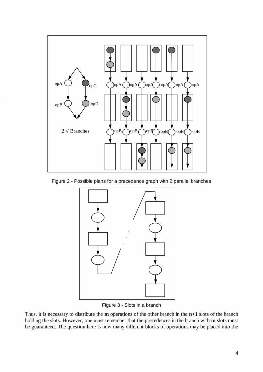
Figure 2 illustrates the possible plans for two parallel branches with two operations each. The

parallel grouping will give as result 6 plans (Nplan = 6) with 4 operations. Figure 2 helps to

understand the basic idea to obtain the number of plans. In any case, we will have four operations for

the plan since all operations are necessary. Our goal is to compute how many plans will exist without

generating them.

The basic idea is to expand one branch on another one. For example considering the left branch of

the figure we will have three places (slots) where the operations of the right branch can be placed

(before both operations, between op1 and op2 and after both operations). These slots are

represented by rectangles in the possible plans. Generally, if we have N operations in one branch we

will have N+1 slots (see Figure 3).

a) Serial operations b) Parallel branches of operations

4

Figure 2 - Possible plans for a precedence graph with 2 parallel branches

Figure 3 - Slots in a branch

Thus, it is necessary to distribute the m operations of the other branch in the n+1 slots of the branch

holding the slots. However, one must remember that the precedences in the branch with m slots must

be guaranteed. The question here is how many different blocks of operations may be placed into the

opA opA opA opA opA opA

opB opB opB opB opB opB

opB

opC opA

2 // Branches

opD

.

.

.

5

slots. Table 1 shows several possibilities of distribution of the m operations (1 m 6) grouped by

blocks. In the table we consider that opi precedes opi+1.

Table 1 - Grouping m operations in blocks (1 m 6)

M 1 block 2 blocks 3 blocks 1 {op1}

2 {op1,op2} {op1} {op2}

3 {op1,op2,op3} {op1} {op2,op3}

{op1,op2} {op3}

{op1} {op2} {op3}

4 {op1,op2,op3,op4} {op1} {op2,op3,op4}

{op1,op2} {op3,op4}

{op1,op2,op3} {op4}

{op1} {op2} {op3,op4}

{op1} {op2,op3} {op4}

{op1,op2} {op3} {op4}

5 {op1,op2,op3,op4,op5} {op1} {op2,op3,op4,op5}

{op1,op2} {op3,op4,op5}

{op1,op2,op3} {op4,op5}

{op1,op2,op3,op4} {op5}

{op1} {op2} {op3,op4,op5}

{op1} {op2,op3,op4} {op5}

{op1,op2,op3} {op4} {op5}

{op1,op2} {op3,op4} {op5}

{op1,op2} {op3} {op4,op5}

{op1} {op2,op3} {op4,op5}

6 {op1,op2,op3,op4,op5,op6} {op1} {op2,op3,op4,op5,op6}

{op1,op2,op3,op4,op5} {op6}

{op1,op2} {op3,op4,op5,op6}

{op1,op2,op3,op4} {op5,op6}

{op1,op2,op3} {op4,op5,op6}

{op1} {op2} {op3,op4,op5,op6}

{op1} {op2,op3,op4,op5} {op6}

{op1,op2,op3,op4} {op5} {op6}

{op1} {op2,op3} {op4,op5,op6}

{op1} {op2,op3,op4} {op5,op6}

{op1,op2} {op3} {op4,op5,op6}

{op1,op2} {op3,op4,op5} {op6}

{op1,op2,op3} {op4} {op5,op6}

{op1,op2,op3} {op4,op5} {op6}

{op1,op2} {op3,op4} {op5,op6}

M 4 block 5 blocks 6 blocks 1 2 3 4 {op1} {op2} {op3} {op4}

5 {op1} {op2} {op3} {op4,op5}

{op1} {op2} {op3,op4} {op5}

{op1} {op2,op3} {op4} {op5}

{op1,op2} {op3} {op4} {op5}

{op1} {op2} {op3} {op4} {op5}

6 {op1} {op2} {op3} {op4,op5,op6}

{op1} {op2} {op3,op4,op5} {op6}

{op1} {op2,op3,op4} {op5} {op6}

{op1,op2,op3} {op4} {op5} {op6}

{op1} {op2} {op3,op4} {op5,op6}

{op1} {op2,op3} {op4} {op5,op6}

{op1} {op2,op3} {op4,op5} {op6}

{op1,op2} {op3,op4} {op5} {op6}

{op1,op2} {op3} {op4,op5} {op6}

{op1,op2} {op3} {op4} {op5,op6}

{op1} {op2} {op3} {op4} {op5,op6}

{op1} {op2} {op3} {op4,op5} {op6}

{op1} {op2} {op3,op4} {op5} {op6}

{op1} {op2,op3} {op4} {op5} {op6}

{op1,op2} {op3} {op4} {op5} {op6}

{op1} {op2} {op3} {op4} {op5} {op6}

If we look to the table, we can see that for grouping m operations in i blocks we will have Cim1

1

groups. The i blocks can be placed into the slots. Since we have n+1 slots, it is easy to conclude that

for i blocks we have Cin1 possible combinations. Thus, for expanding one branch with m

6

operations, grouped in i blocks, on another branch with n operations we have C Cin

im11

1 possible

combinations. However, since the number of blocks i varies from 1 to the minimum between m and

n+1, the total amount of combinations of operations in two parallel branches is:

C Cin

im

i

n m

1

11

1

1min( , )

combinations (subplans) with n+m operations.

The used reasoning was to expand the branch with m operations on the branch with n operations.

The inverse reasoning could be used (to expand the branch with n operations on the branch with m

operations). This corresponds to the right-hand side of the following expression that can be

mathematically proved:

C C C Cin

im

im

in

i

m n

i

n m

1

11 1

11

1

1

1

1 min( , )min( , )

For the example of figure 2 we have m=2, and n=2. Thus, the number of possible plans with these 4

operations is given by:

C C C C C C C Cin

im

i

n m

i ii

11

1

1

13

11

1

2

13

01

23

11 3 1 3 1

min( , )

* *

The first product of the sum corresponds to the possibilities of grouping in one slot (3 possibilities:

before opA and opB; between opA and opB; and after opA and opB) the two operations of the right

branch in one block (only one {opC,opD}). This part corresponds to the following plans (the 3 first

plans of Figure 2):

{opC,opD},opA,opB

opA,{opC,opD},opB

opA,opB,{opC,opD}.

The second product of the sum corresponds to the possibilities of grouping in two slots (3

possibilities: using the first and second slots; using the first and third slots; and using the second and

third slots) the two operations of the right branch in two blocks (only one {opC}, {opD}). This part

corresponds to the following plans (the three last plans of Figure 2):

{opC},opA,{opD},opB

{opC},opA,opB,{opD}

opA,{opC},opB,{opD}.

3- THE PARSE TREE

In order to compute the total number of possible plans of a precedence graph we must group

operations in serial and parallel until the equivalent has been obtained. A parse tree is built to drive

the grouping process.

Let us consider an example for making the object shown in Figure 4, involving 12 operations,

starting with an aluminum cylinder. A lathe can be used to perform the necessary processing

7

operations. The surface of the cylinder must be uniformly adjusted and some facing and turning

operations are necessary. By default, we do not know the order by which the operations must be

done. The sequence of operations will be obtained by the feasibility and geometric constraints

between parts and tools. There are also some processing constraints.

Figure 4 - example

The precedence graph for the above example is shown in Figure 5, considering all feasibility,

geometric (e.g. operation 1 must be done before operation 2) and processing constraints (e.g. for this

type of material we must adjust the surface before starting turning).

Op 1

Op 2 Op 7 Op 8

Op 6Op 3 Op 5

Op 4

Op 9

Op 10

Op 11

Op 0

Figure 5 - Precedence graph for the example

The parse tree for this graph is illustrated in Figure 6 where the terminal nodes are the operations, p

represents parallel operations and s represents serial operations.

The parse tree defines how to proceed in the grouping process to obtain the total number of possible

plans.

8

Figure 6 - Parse Tree of the precedence graph of Figure 5

For this example, the number of possible plans is obtained as follows:

for parallel of {op5, op6}, n=1, m=1 (let us name it as )

21*20

0

2

1

1

1

0

1

2),1min(

1

1

1

1

CCCCCCi

ii

mn

i

m

i

n

i

this means 2 plans ( = 2) with 2 operations (m + n = 2)

for parallel of {op3, }, n=1, m=2 (let us name it as )

* 63*2)1*11*2(*2** 1

1

2

2

1

0

2

1

2

1

1

1

2),1min(

1

1

1

1

CCCCCCCCi

ii

mn

i

m

i

n

i

this means 6 plans ( = 6) with 3 operations (n + m = 3).

Notice that it is necessary to multiply the sum by , since the sum represents the possible

solution for 1 plan of the branch; however for we have 2 plans.

for the serial operations op2, op4, and those of , we have the same number of plans than in , but

with 5 operations, since the parallel has 3 operations

s Op 7 Op 8

p Op 1

s

Op 11 Op 10

s

p Op 0

s

Op 9

Op 4 p Op 2

Op 6 Op 5 Op 3

9

for parallel {op8, s(op2, op4, )}, n=1, m=5 (let us name it as )

* 366*6)4*11*2(*6** 4

1

2

2

4

0

2

1

2

1

4

1

2),1min(

1

1

1

1

CCCCCCCCi

ii

mn

i

m

i

n

i

this means 36 plans ( = 36) with 6 operations (m + n = 6)

for parallel of {op7, }, n=1, m=6 (let us name it as )

2527*36)5*11*2(*36*** 5

1

2

2

5

0

2

1

2

1

5

1

2),1min(

1

1

1

1

CCCCCCCCi

ii

mn

i

m

i

n

i

this means 252 plans with 7 operations (n + m = 7)

for the serial operations op1 and those of , we have the same number of plans of , but with 8

operations, since the parallel has 7 operations

for the serial operations op9, op10 and op11 we have only one plan with 3 operations

for parallel of {s(op9, op10, op11), s(op1, )}, n=3, m=8

7

3

4

4

7

2

4

3

7

1

4

2

7

0

4

1

4

1

7

1

4),1min(

1

1

1

1 ****1 CCCCCCCCCCCCi

ii

mn

i

m

i

n

i

41580165*252)35*121*47*61*4(*252

Therefore, since this is the last grouping, the total number of possible plans for the task is 41 580.

Once the number of plans has been achieved, one may decide which policy to use in order to

generate the plans. If the number of plans is reduced then the generation of all plans is possible in

order to give to the user the possibility to choose by him in a set of few solutions. If the number of

plans is high then one may decide to adopt one of the following policies: the fast generation of N

plans or the generation of the best N plans according with the time execution criterion. In this way,

the user will have the possibility to analyze only a small number of good possibilities. The experience

shows that usually the best plan to achieve a compromise of constraints is in the set of the best plans

according to the time execution criterion.

4- EXECUTION PLAN

The plan generation is achieved considering all precedence relations (obtained from constraints)

represented by the graph and the policy chosen as described in chapter 3. Note that, in this case, only

feasible plans are generated.

The algorithm used to generate the plan [2] consider, for each operation, the time needed for each

operation as well as the time for changing from one operation to another (e.g., change the tool, wait

a certain time before a specific operation due to the involved process and so on). In this algorithm,

10

the configuration of the manufacturing system is also considered, since the sequence of operations is

important due to the time needed for changing from one operation to another.

Then it is possible to select the best plan (if that policy was chosen) considering time execution as

criterion, since all times involved in the operations, tools' changing and setup are considered. In the

example, as the number of different operations is small and the number of total operations is bigger,

the main problems (concerning choice of best algorithm) are not the operations time, but the tools'

changing and setup times. This is why the best plan is the one that minimizes the number of tools'

changing operations and times needed to move tools from one operation to another.

The best plan, for the example above, is: 0 - 1 - 8 - 2 - 3 - 7 - 6 - 5 - 4 - 9 - 10 - 11.

The next step is the generation of the program. The configuration of the manufacturing system must

also be considered, since programs should be generated for each machine. This corresponds to the

areas of Computer Aided Process Planning and CAD/CAM. The reader can find some good

references of this kind of works in [10-14].

For the example of Figure 4, the code for the lathe is presented at Figure 7.

O0004

M62

M39

G99 G21 G00 X30 Z20

M06 T0303

G00 X28 Z2

G71 U0.1 R0.1

G71 P01 Q02 U0.5 W0.5 F0.2

N01 G01 X26

N02 G01 Z-45

G00 X30 Z20

G71 U0.1 R0.1

G71 P05 Q06 U0.1 W0.1 F0.1

N05 G01 X24

N06 G01 Z-45

G70 P05 Q06

G00 X23 Z1

G01 X24 Z-1

G00 X30 Z20

M06 T0505

G00 X25 Z-40

G72 U0.1 R0.1

G72 P07 Q08 U0.1 W0.1 F0.1

N07 G00 X15

N08 G01 X20 Z-40

G70 P07 Q08

G00 X25

G72 U0.1 R0.1

G72 P09 Q10 U0.1 W0.1 F0.1

N09 G00 X15

N10 G02 X15 Z-35 R8

G70 P09 Q10

G00 X30 Z20

M06 T0101

G00 X25 Z-15

G71 U0.1 R0.1

G71 P11 Q12 U0.1 W0.1 F0.1

N11 G00X24

N12 G03 X18 Z-20 R5

G70 P11 Q12

G00 X25 Z-15

G71 U0.1 R0.1

G71 P13 Q14 U0.1 W0.1 F0.1

N13 G00X24

N14 G01 X18 Z-23

G70 P13 Q14

G00 X25 Z-29

G72 U0.1 R0.1

G72 P15 Q17 U0.1 W-0.1 F0.1

N15 G00 Z-29

N16 G00 Z-24 W1

N17 G01 X18 Z-23

G70 P15 Q17

G00 X25 Z-24

G72 U0.1 R0.1

G72 P18 Q20 U0.1 W-0.1 F0.1

N18 G00 Z-29

N19 G00 Z-24 W1

N20 G01 X15 Z-25

G70 P18 Q20

G00 X25 Z1

G72 U0.1 R0.1

G72 P21 Q22 U0.1 W-0.1 F0.1

N21 G00 Z-4 W2

N22 G01 X0

G70 P21 Q22

G00 X30 Z20

M06 T0404

M03 S1200

G00X0 Z2

G01 Z-14 F0.05

G01 Z2

G00 X30 Z20

M06 T0202

G00 X0 Z0

G71 U0.1 R0.1

G71 P23 Q25 U0.1 W0.1 F0.1

N23 G00 X16

N24 G01 X16 Z-12

N25 G01 X12 Z-14

G70 P23 Q25

G00 X26 Z20

M09 G00 X25 Z1

M05 G04 X5

M38

M64

M15

%

Figure 7 - Program for a GE FANUC SERIES OT lathe

5- CONCLUSIONS

In this paper, we have presented a method for computing the complexity of a precedence graph for

manufacturing or assembly tasks. As the core of the method we created the slot-block theory, that

allows to group branches of precedence graphs in order to know how many possible combinations of

0

9

10

5

4

7

6

2

3

11

1

8

11

operations (subplans) exists. A parse tree defines how to proceed in the grouping process to obtain

the total number of possible plans of a precedence graph.

The method presented in this paper is implemented in software. Using the software one can rapidly

obtain the number of plans of a specific precedence graph, and decide which plan generation

algorithm to use. The decision about which algorithm to use depends on the total number of plans as

well as on the purposes of the planning system (on-line versus off-line, strategic versus tactical or

reactive).

This work shows the impact of Information Technology on industrial processes. Besides the

computer aided process planning part of our work that is not described here (see references [2] - [7])

we introduced a new method for the complexity analysis of precedence graphs. This method is

implemented in software.

With our computer application for complexity analysis, we are able to know if we are in the presence

of a combinatory explosion problem or not. Therefore, the software can select, automatically, the

search method to use. The possible methods are the generation of all plans, the fast generation of one

or more good plans or the generation of the best plan (or even the N best plans). All these search

methods are implemented also in software.

Further work on this method will be to consider several resources to execute the manufacturing and

assembly task. In this case, some different plans are equivalent due to the parallelism during task

execution. Temporal reasoning is important for this kind of study.

Another future direction is the integration with work being developed in the area of production

planning and scheduling [15-16].

ACKNOWLEDGEMENTS

The authors of this paper would like to acknowledge FLAD (the Portuguese-American Foundation

for the Development) for the support of Project 443/93 (SFF - Flexible Manufacturing Systems).

The authors would like to acknowledge JNICT (the Joint National Institute for Scientific Research

and Technology) for the support of Projects 2556/95 (SAPPIOP - Industrial Process Planning

Support System) and 2551/95 (SAD/3PE - Decision Support System for Production Planning

considering due dates).

BIBLIOGRAPHY

[1] S. Gottschlich, C. Ramos, D. Lyons - Assembly and Task Planning: A Taxonomy, IEEE

Robotics and Automation Magazine, vol. 1, n. 3, pp. 4-12, September 1994

[2] J. Rocha, C. Ramos - Plan Representation and Heuristic Generation of Operation Sequences for

Manufacturing Tasks, International Conference on Data and Knowledge Systems for

Manufacturing and Engineering - DKSME'96, Tempe AZ (USA), 1996

[3] J. Rocha, C. Ramos - Plan Representation and Generation for Manufacturing Tasks, First IEEE

International Symposium on Assembly and Task Planning, Pittsburgh (USA), 1995

12

[4] J. Rocha, C. Ramos - TPMS: a system for sequencing operations in Process Planning, Eighth

International Conference on Industrial & Engineering Applications of Artificial Intelligence

and Expert Systems, Melbourne (Australia), 1995

[5] J. Rocha, C. Ramos, Z. Vale - Sequencing Operations for Process Planning, The Practical

Application of PROLOG Conference, Paris (France), 1995

[6] J. Rocha, C. Ramos, Z. Vale - Heuristic Generation of Operation Sequences for Process Plans,

Advanced Summer Institute of Network of Excellence in Intelligent Control and Integrated

Manufacturing Systems, ASI'95, Lisbon, 1995

[7] J. Rocha, C. Ramos, Task Planning for Flexible and Agile Manufacturing Systems, IEEE/RSJ

International Conference on Intelligent Robots and Systems - IROS'94, Munich (Germany),

1994, invited paper

[8] L. Homem de Mello - Task sequence planning for robotic assembly, PhD Dissertation, Carnegie

Mellon University, 1989

[9] S. Gupta, D. Nau - Optimal Block's World Solutions are N-P, Technical Report, Computer

Science Department, University of Maryland, 1990.

[10] C. C. Hayes - MACHINIST: A Process Planner for Manufacturability Analysis, 1995

[11] J. Tulkoff - CAPP - Computer Aided Process Planning, Computer and Automated Systems

Association of SME, Michigan, 1985

[12] L. Figueiredo, Conversion and Execution of Process Plans, Master Thesis, University of Porto,

1996

[13] A. Kusiak. - Intelligent Manufacturing Systems, Prentice-Hall International Series in Industrial

and Systems Engineering, 1990

[14] D. Das, S. Gupta, and D. Nau - Reducing cost set-up by automated generation of redesign

suggestions, ASME Computers in Engineering Conference, 1994

[15] C. Ramos, A. Almeida, Z. Vale - Scheduling Manufacturing Orders with Due Dates acting as

real deadlines, Advanced Summer Institute of Network of Excellence in Intelligent Control and

Integrated Manufacturing System, ASI'95, Lisbon, 1995

[16] C. Ramos - An Architecture and a Negotiation Protocol for the Dynamic Scheduling of

Manufacturing Systems, IEEE International Conference on Robotics and Automation -

ICRA´94, San Diego (USA), pp. 3161-3166, 1994