On the computational complexity of cut-reduction

arX

iv:0

712.

1499

v1 [

cs.L

O]

10

Dec

200

7

On the computational complexity of

cut-reduction

Klaus Aehlig

Computer Science

Swansea University

Swansea SA2 8PP, UK

[email protected]

Arnold Beckmann

Computer Science

Swansea University

Swansea SA2 8PP, UK

[email protected]

February 2, 2008

Abstract

We investigate the complexity of cut-reduction on proof notations,in particular identifying situations where cut-reduction operates feasibly,i.e., sub-exponential, on proof notations. We then apply the machineryto characterise definable search problem in Bounded Arithmetic.

To explain our results with an example, let E(d) denote Mints’ con-tinuous cut-reduction operator which reduces the complexity of all cutsof a propositional derivation d by one level. We will show that if all sub-proofs of d can be denoted with notations of size s, and the height of d

is h, then sub-proofs of the derivation E(d) can be denoted by notationsof size h · (s +O(1)). Together with the observation that determining thelast inference of a denoted derivation as well as determining notations forimmediate sub-derivations is easy (i.e., polynomial time computable), wecan apply this result to re-obtain that the Σb

i -definable functions of theBounded Arithmetic theory Si

2 are in the i-th level of the polynomial time

hierarchy of functions FPΣbi−1 .

1 Introduction and Related Work

Since Gentzen’s invention of the “Logik Kalkul” LK and the proof of his “Haupt-satz” [Gen35a, Gen35b], cut-elimination has been studied in many papers onproof theory. Mints’ invention of continuous normalisation [Min78, KMS75]isolates operational aspects of normalisation, that is the manipulations on (in-finitary) propositional derivations. These operational aspects are described in-dependently of the system’s proof theoretic complexity, but at the expense ofintroducing the void logical rule of repetition to balance derivation trees.

Γ (R)Γ

1

http://arXiv.org/abs/0712.1499v1

[email protected]

[email protected]

Note that this rule is both logically valid and preserves the sub-formula property,which in particular means that it does not harm computational tasks related toderivations as long as it does not occur too often.

It is well-known that, using (R), the cut-elimination operator becomes aprimitive recursive function which is continuous w.r.t. the standard metric oninfinitary trees: the normalisation procedure requires only as much informa-tion of the input as it produces output, using (R) as the last inference rule ofthe normal derivation, if the result cannot immediately be determined (“pleasewait”).

In fact, associating some of the repetition rules with computation stepsbounds for the simply-typed lambda calculus can be obtained that bound thesum of the number of computation steps and the size of the output [AJ05],strengthening earlier results by Beckmann [Bec01]. Using Schutte’s ω-rule [Sch51]this method can also be applied to Godel’s [God58] system T .

In this report, we will re-examine this situation. We will show that the cut-reduction operator can be understood as a polynomial time operation naturalway, see Observation 9.12. We will work with proof notations which give implicitdescriptions of (infinite) propositional proofs: a proof notation system will be aset which is equipped with some functions, most importantly two which computethe following tasks:

• Given a notation h, compute the last inference tp(h) in the denoted proof.

• Given a notation h and a number i ∈ N, compute a notation h[i] for thei-th immediate sub-derivation of the derivation denoted by h.

Implicit proof notations given in this way uniquely determine a propositionalderivation tree, by exploring the derivation tree from its root and determiningthe inference at each node of the tree. The cut-reduction operator will bedefined on such implicitly described derivation trees. For this, we build onBuchholz’ technical very smooth approach to notation systems for continuouscut-elimination [Buc91, Buc97]. Our main result of the first part of the report inparticular implies the following statement, as can be seen from Corollary 9.11.Let 2n(x) denote the n-fold iteration of exponentiation 2x.

Let d be some propositional derivation, and assume that all sub-proofs of d can be denoted with notations of size bounded by s,and that the height of d is h. Then, all sub-proofs of the derivationobtained from d by reducing the complexity of cut-formulae by kcan be denoted by notations of size bounded by 2k−1(2h) · s.

Observe that the size of notations is exponential only in the height of the originalderivation. In the second part of this report we will identify situations occurringin proof-theoretical investigations of Bounded Arithmetic where this height isbounded by an iterated logarithm of some global size parameter, making thesesizes feasible.

2

Bounded Arithmetic has been introduced by Buss [Bus86] as theories ofarithmetic with a strong connection to computational complexity. For sakeof simplicity of this introduction, we will concentrate only on the BoundedArithmetic theories Si

2 by Buss [Bus86]. These theories are given as first or-der theories of arithmetic in a language which suitably extends that of PeanoArithmetic where induction is restricted in two ways. First, logarithmic induc-tion is considered which only inducts over a logarithmic part of the universe ofdiscourse.

ϕ(0) ∧ (∀x)(ϕ(x) → ϕ(x + 1)) → (∀x)ϕ(|x|) .

Here, |x| denotes the length of the binary representation of the natural num-ber x, which defines a kind of logarithm on natural numbers. Second, theproperties which can be inducted on, must be described by a suitably restricted(“bounded”) formula. The class of formulae used here are the Σb

i -formulaewhich exactly characterise Σp

i , that is, properties of the i-th level of the poly-nomial time hierarchy of predicates. The theory’s Si

2 main ingredients are theinstances of logarithmic induction for Σb

i formulae.Let a (multi-)function f be called Σb

j -definable in Si2, if its graph can be

expressed by a Σbj -formula ϕ, such that the totality of f , which renders as

(∀x)(∃y)ϕ(x, y), is provable from the Si2-axioms in first-order logic. The main

results characterising definable (multi-) functions in Bounded Arithmetic arethe following.

• Buss [Bus86] has characterised the Σbi -definable functions of Si

2 as FPΣbi−1 ,

the i-th level of the polynomial time hierarchy of functions.

• Krajıcek [Kra93] has characterised the Σbi+1-definable multi-functions of

Si2 as the class FPΣb

i [wit,O(log n)] of multi-functions which can be com-puted in polynomial time using a witness oracle from Σp

i , where the num-ber of oracle queries is restricted to O(log n) many (n being the length ofthe input).

• Buss and Krajıcek [BK94] have characterised the Σbi−1-definable multi-

functions of Si2 as projections of solutions to problems from PLSΣb

i−2 , whichis the class of polynomial local search problems relativised to Σp

i−2-oracles.

We will re-obtain all these definability characterisations by one unifyingmethod using the results from the first part of this report in the followingway. First, we will define a suitable notation system HBA for propositionalderivations which are obtained by translating Bounded Arithmetic proofs. Thepropositional translation used here is well-known in proof-theoretic investiga-tions; the translation has been described by Tait [Tai68], and later was inde-pendently discovered by Paris and Wilkie [PW85]. In the Bounded-Arithmeticworld it is known as the Paris-Wilkie translation.

Applying the machinery from the first part we obtain a notation systemCHBA of cut-elimination for HBA. CHBA will have the property that its implicit

3

descriptions, most notably the functions tp(h) and h[i] mentioned above, willbe polynomial time computable.

This allows us to formulate a general local search problem on CHBA whichis suitable to characterise definable multi-functions for Bounded Arithmetic.Assume that (∀x)(∃y)ϕ(x, y), describing the totality of some multi-function, isprovable in some Bounded Arithmetic theory. Fix a particularly nice formalproof p of this. Given N ∈ N we want to describe a procedure which finds someK such that ϕ(N,K) holds. Invert the proof p of (∀x)(∃y)ϕ(x, y) to a proofof (∃y)ϕ(x, y) where x is fresh a variable, then substitute N for all occurrencesof x. This yields a proof of (∃y)ϕ(N, y). Adding an appropriate number ofcut-reduction operators we obtain a proof with all cut-formulae of (at most) thesame logical complexity as ϕ. It should be noted that a notation h(N) for thisproof can be computed in time polynomial in N .

The general local search problem which finds a witness for (∃y)ϕ(N, y) cannow be characterised as follows. Its instance is given by N . The set of solutionsare those notations of a suitable size, which denote a derivation having theproperty that the derived sequent is equivalent to (∃y)ϕ(N, y) ∨ ψ1 ∨ · · · ∨ ψl

where all ψi are “simple enough” and false. An initial solution is given byh(N). A neighbour to a solution h is a solution which denotes an immediatesub-derivation of the derivation denoted by h, if this exists, and h otherwise. Thecost of a notation is the height of the denoted derivation. The search task is tofind a notation in the set of solutions which is a fixpoint of the neighbourhoodfunction. Obviously, a solution to the search task must exist. In fact, anysolution of minimal cost has this property. Now consider any solution to thesearch problem. It must have the property, that none of the immediate sub-derivations is in the solution space. This can only happen if the last inferencederives (∃y)ϕ(N, y) from a true statement ϕ(N,K) for some K ∈ N. Thus Kis a witness to (∃y)ϕ(N, y), and we can output K as a solution to our originalwitnessing problem.

Depending on the complexity of logarithmic induction present in the BoundedArithmetic theory we started with, and the level of definability, we obtain lo-cal search problems defined by functions of some level of the polynomial timehierarchy, and different bounds to the cost function. For example, if we startwith the Σb

i -definable functions of Si2, we obtain a local search problem defined

by properties in FPΣbi−1 , where the cost function is bounded by |N |O(1). Thus,

by following the canonical path through the search problem which starts atthe initial value and iterates the neighbourhood function, we obtain a path of

polynomial length, which describes a procedure in FPΣbi−1 to compute a witness.

Other research related to our investigations is a paper by Buss [Bus04] whichalso makes use of the Paris-Wilkie translation to obtain witnessing results bygiving uniform descriptions of translated proofs. However, Buss’ approach doesnot explicitely involve cut-elimination. Dynamic ordinal analysis [Bec03, Bec06]characterises the heights of propositional proof trees obtained via the Paris-Wilkie translation and cut-reduction. Therefore, it is not surprising that the

4

bounds obtained by dynamic ordinal analysis coincide with the bounds on costfunctions we are exploiting here.

The potential of our approach to the characterisations of definable searchproblems via notation systems is that it may lead to characterisations of sofar uncharacterised definable search problems, most notably the Σb

1-definablesearch problems in Si

2 for i ≥ 3.

2 Proof Systems

Let S be a set. The set of all subsets of S will be denoted by P(S), the set ofall finite subsets of S will be denoted by Pfin(S).

Definition 2.1 (sequent). Let F be a set (of formulae), ≈ a binary relation onF (identity between formulae), and rk: P(F)×F → N a function (rank). A se-quent over F ,≈, rk is a finite subset of F . We use Γ,∆, . . . as syntactic variablesto denote sequents. With ≈∆ we denote the set {A ∈ F : (∃B ∈ ∆)A ≈ B}.

We usually write A1, . . . , An for {A1, . . . , An} and A,Γ,∆ for {A} ∪ Γ ∪ ∆,etc. We always write C-rk(A) instead of rk(C, A).

We repeat standard Buchholz notation for proof systems [Buc97].

Definition 2.2. A proof system S over F ,≈, rk is given by

• a set of formal expressions called inference symbols (syntactic variable I);

• for each inference symbol I an ordinal |I| ≤ ω, a sequent ∆(I) and afamily of sequents (∆ι(I))ι<|I|.

Proof systems may have inference symbols of the form CutC for C ∈ F ;these are called “cut inference symbols” and their use will (in Definition 2.4) bemeasured by the C-cut rank.

Notation 2.3. By writing. . .∆ι . . . (ι < I)

(I)∆

we declare I as an infer-

ence symbol with |I| = I, ∆(I) = ∆, ∆ι(I) = ∆ι. If |I| = n we write∆0 ∆1 . . . ∆n−1

∆instead of

. . .∆ι . . . (ι < I)

∆.

Definition 2.4 (Inductive definition of S-quasi derivations). If I is an inferencesymbol of S, and (dι)ι<|I| is a sequence of S-quasi derivations, then d :=

5

I(dι)ι<|I| is an S-quasi derivation with

Γ(d) := ∆(I) ∪⋃

ι<|I|

(Γ(dι) \ ≈∆ι(I)) (endsequent of d)

last(d) := I (last inference of d)

d(ι) := dι for ι < |I| (sub-derivation)

C-crk(d) := sup({C-rk(I)} ∪ {C-crk(dι) : ι < |I|}) (cut-rank of d)

where C-rk(I) :=

{C-rk(C) + 1 if I = CutC

0 otherwise

hgt(d) := sup {hgt(dι) + 1: ι < |I|} (height of d)

sz(d) := (∑

ι<|I|

sz(dι)) + 1 (size of d)

3 The infinitary proof system

Definition 3.1. Let C = {⊤,⊥,∧,∨} be the set of (symbols for) connectives

for infinitary logic. Their arity is given by |⊤| = |⊥| = 0 and |∧| = |

∨| = ω. We

define a negation of the connectives according to the de Morgan laws: ¬(⊤) = ⊥,¬(⊥) = ⊤, ¬(

∧) =

∨, and ¬(

∨) =

∧.

Definition 3.2. The set of all infinitary formulae L∞ together with their rankis inductively defined by the clause: if c ∈ C and Aι ∈ L∞ for ι < |c| thenc(Aι)ι<|c| ∈ L∞ and C-rk(c(Aι)ι<|c|) = supι<|c|(C-rk(Aι) + 1).

Notation

We denote ⊤() by ⊤ and ⊥() by ⊥.

Definition 3.3. ¬ denotes the operation on L∞ which computes negation ac-cording to the de Morgan rules, i.e.

¬(c(Aι)ι<|c|

):= ¬(c)

(¬(Aι)

)ι<|c|

Definition 3.4. The set of all infinitary formulae of finite rank is denoted withF∞. The identity between F∞-formulae is the “true” set-theoretic equality.

Definition 3.5. The infinitary proof system S∞ is the proof system over F∞

which is given by the following set of inference symbols:

(Ax)⊤

. . . Aι . . . (ι < ω)(∧

A)A

for A =∧

(Aι)ι<ω ∈ F∞

Ai(∨i

A)A

for A =∨

(Aι)ι<ω ∈ F∞ and i < ω

6

C ¬C(CutC)∅

for C ∈ F∞

∅(Rep)

∅

Definition 3.6. The S∞-derivations are the S∞-quasi derivations.

With a S∞-derivation d = I(dι)ι<|I| we can associate a function from N<ω

to S∞ by letting d(〈〉) := last(d) and

d(〈i〉⌢ s) :=

{di(s) if i < |I|

Ax otherwise

4 Notation system for infinitary formulae

Definition 4.1. A notation system for (infinitary) formulae is a set F of “for-mulae”, together with four functions tp : F → {⊤,⊥,

∧,∨}, ·[·] : F × N → F ,

¬ : F → F , and rk: P(F) × F → N called “outermost connective”, “sub-formula”, “negation” and “rank”, and a relation ≈ ⊆ F × F called “inten-sional equality”, such that tp(¬(f)) = ¬(tp(f)), ¬(f)[n] = ¬(f [n]), C-rk(f) =C-rk(¬f), C-rk(f [n]) < C-rk(f) for n < | tp(f)|, and f ≈ g implies tp(f) = tp(g),f [n] ≈ g[n], ¬(f) ≈ ¬(g) and C-rk(f) = C-rk(g).

It should be noted that if F is a notation system for formulae, then so isF/ ≈ in the obvious way; moreover, in F/ ≈ the intensional equality is trueequality in the quotient. The reason why we nevertheless explicitly consideran (intensional) equality relation is that we are interested in the computationalcomplexity of notation systems and therefore prefer to take notations as thestrings that arise naturally, rather than working on the quotient. Note thatthe latter would require us to compute canonical representations anyway andso would just push the problem to a different place.

It should also be noted that the intensional equality is truly intensional.Two formulae are only equal, if they are given to us as being equal. The obvi-ous extensional equality would be the largest bisimulation, that is, the largestrelation ∼⊂ F ×F satisfying f ∼ g → tp(f) = tp(g) ∧ f [n] ∼ g[n] ∧ C-rk(f) =C-rk(g) ∧ ¬f ∼ ¬g. However, as most extensional concepts, the largest bisimu-lation is undecidable in almost all interesting cases and therefore not suited foran investigation of effective notations.

Definition 4.2. Let F = (F , tp, ·[·], rk,≈) be a notation system for infinitaryformulae. The interpretation [[f ]]∞ of f ∈ F is inductively defined as

[[f ]]∞ = tp(f)([[f [ι]]]∞)ι<| tp(f)|

Observation 4.3. The following properties hold.

1. f ∼ g ⇔ [[f ]]∞ = [[g]]∞,

2. f ≈ g ⇒ [[f ]]∞ = [[g]]∞.

7

5 Semiformal proof systems

Let F = (F , tp, ·[·], rk,≈) be a notation system for infinitary formulae.

Definition 5.1. The semiformal proof system SF over F is the proof systemover F which is given by the following set of inference symbols:

(AxA)A for A ∈ F with tp(A) = ⊤

. . . C[n] . . . (n ∈ N)(∧

C)C

for C ∈ F with tp(C) =∧

C[i](∨i

C)C

for C ∈ F with tp(C) =∨

and i ∈ N

C ¬C(CutC)∅

for C ∈ F with tp(C) ∈ {⊤,∧}

∅(Rep)

∅

Abbreviations

For tp(C) ∈ {⊥,∨} let

C ¬C(CutC)∅

denote¬C C(Cut¬C)

∅.

Definition 5.2. The SF -derivations are the SF -quasi derivations.

Later in our applications, we will be concerned only with derivations offinite height, for which we can formulate slightly sharper upper bounds on cut-reduction than in the general (infinite) case (2α versus 3α). Thus, from now onwe will restrict attention to derivations of finite height only.

Definition 5.3. Let d ⊢αC,m Γ denote that d is an SF -derivation with Γ(d) ⊆

≈Γ, C-crk(d) ≤ m, and hgt(d) ≤ α < ω .

Definition 5.4. The interpretation [[d]]∞ of a SF -derivation d = I(dι)ι<|I| isdefined as

[[d]]∞ := [[I]]∞([[dι]]∞)ι<|I|

where [[I]]∞ is defined by

[[AxA]]∞ := Ax

[[∧

A]]∞ :=∧

[[A]]∞

[[∨i

A]]∞ :=∨i

[[A]]∞

[[CutC ]]∞ := Cut[[C]]∞

[[Rep]]∞ := Rep

Observation 5.5. Γ([[d]]∞) ⊆ [[Γ(d)]]∞

Proof. Induction on d. The “⊆”, instead of the expected “=” is due to thefact, that only formulae are removed from the conclusion that are intensionallyequal; compare also Observation 4.3.

8

6 Cut elimination for semiformal systems

Let F = (F , tp, ·[·], rk,≈) be a notation system for infinitary formulae, and SF

the semiformal proof system over F . We define Mints’ continuous cut-reductionoperator [Min78, KMS75] following the description given by Buchholz [Buc91].The only modification is our explicit use of intensional equality.

Theorem 6.1 (and Definition). Let C ∈ F with tp(C) =∧

, and k < ω be given.We define an operator Ik

C such that: d ⊢αC,m Γ, C ⇒ Ik

C(d) ⊢αC,m Γ, C[k].

Proof by induction on the build-up of d: W.l.o.g. we may assume that Γ = Γ(d)\≈{C}.

Case 1. last(d) ∈ {∧

D : D ≈ C}. Then

IkC(d) := Rep(Ik

C(d(k)))

is a derivation as required.

Case 2. I := last(d) /∈ {∧

D : D ≈ C}. Then

IkC(d) := I(Ik

C(d(i)))i<|I|


Theorem 6.2 (and Definition). Let C ∈ F with tp(C) ∈ {⊤,∧} be given.

We define an operator RC such that: d0 ⊢αC,m Γ, C & d1 ⊢β

C,m Γ,¬C

& C-rk(C) ≤ m ⇒ RC(d0, d1) ⊢α+βC,m Γ.

Proof by induction on the build-up d: W.l.o.g. we may assume that Γ = (Γ(d0)\≈{C}) ∪ (Γ(d1) \ ≈{¬C}). Let I = last(d1).

Case 1. ∆(I)∩≈{¬C} = ∅. Then ∆(I) ⊆ Γ and d1(i) ⊢βi

C,m Γ,¬C,∆i(I) with

βi < β for all i < |I|. By induction hypothesis we obtain RC(d0, d1(i)) ⊢α+βi

C,m

Γ,∆i(I) for i < |I|. Hence

RC(d0, d1) := I(RC(d0, d1(i)))i<|I|


Case 2. ∆(I)∩≈{¬C} 6= ∅. Then tp(C) 6= ⊤, because otherwise there is someD ∈ ∆(I) with tp(D) = ⊥, but this is not satisfied by any of the inferencesymbols of the semiformal system SF . Hence tp(C) =

∧. We obtain that

I =∨k

D for some k ∈ N and D ≈ ¬C, and d1(0) ⊢β0

C,m Γ,¬C,¬C[k] with

β0 < β. By induction hypothesis we obtain RC(d0, d1(0)) ⊢α+β0

C,m Γ,¬C[k]. The

Inversion Theorem shows IkC(d0) ⊢α

C,m Γ, C[k]. Now C-rk(C[k]) < C-rk(C) ≤ m,hence

RC(d0, d1) := CutC[k](IkC(d0),RC(d0, d1(0)))


9

Theorem 6.3 (and Definition). We define an operator E such that:d ⊢α

C,m+1 Γ ⇒ E(d) ⊢2α−1C,m Γ.

Proof by induction on the build-up of d: W.l.o.g. we may assume that Γ = Γ(d).

Case 1. last(d) = CutC . Then C-rk(C) ≤ m and d(0) ⊢α0

C,m+1 Γ, C and

d(1) ⊢α0

C,m+1 Γ,¬C with α0 < α. By induction hypothesis we obtain E(d(0)) ⊢2α0−1C,m

Γ, C and E(d(1)) ⊢2α0−1C,m Γ,¬C.

Case 1.1. tp(C) ∈ {⊤,∧}, then by the last Theorem RC(E(d(0)),E(d(1))) ⊢2·2α0−2

C,m

Γ, andE(d) := Rep(RC(E(d(0)),E(d(1))))


Case 1.2. tp(C) /∈ {⊤,∧}, then R¬C(E(d(1)),E(d(0))) ⊢2·2α0−1

C,m Γ. Continueas before.

Case 2. I := last(d) 6= CutC . Then

E(d) := I(E(d(i)))i<|I|

is as required.

Remark 6.4. Immediately from the definition we note that the operators I, R,and E only inspects the last inference symbol of a derivation to obtain the lastinference symbol of the transformed derivation. It should be noted that thiscontinuity would not be possible without the repetition rule.

7 Notations for derivations and cut-elimination

Let F be a notation system for formulae, and SF the semiformal proof systemover F from Definition 5.1.

Definition 7.1. A notation system for SF is a set H of notations and functionstp: H → SF , ·[·] : H × N → H, Γ : H → Pfin(F), crk : P(F) × H → N, ando, |·| : H → N\{0} called denoted last inference, denoted sub-derivation, denotedend-sequent, denoted cut-rank, denoted height and size, such that C-crk(h[n]) ≤C-crk(h), tp(h) = CutC implies C-rk(C) < C-crk(h), o(h[n]) < o(h) for n <| tp(h)|, and the following local faithfulness property holds for h ∈ H:

∆(tp(h)) ∪⋃

ι<| tp(h)|

(Γ(h[ι]) \ ≈∆ι(tp(h)))

)⊆ ≈Γ(h) .

Proposition 7.2.

Γ(h[j]) ⊆ ≈(Γ(h) ∪ ∆j(tp(h))

)

10

Definition 7.3. Let H = (H, tp, ·[·], o, |·|) be a notation system for SF . Theinterpretation [[h]] of h ∈ H is inductively defined as the following SF -derivation:

[[h]] := tp(h)([[h[n]]])n<| tp(h)|

Observation 7.4. For h ∈ H we have

last([[h]]) = tp(h)

[[h]](ι) = [[h[ι]]] for ι < | tp(h)|

Γ([[h]]) ⊆ ≈Γ(h)

We now extend a notation system H for SF to notation system for cut-elimination on H, by adding notations for the operators I, R and E from theprevious section.

Definition 7.5. The notation system CH for cut-elimination on H is given bythe set of terms CH which are inductively defined by

• H ⊂ CH,

• h ∈ CH, C ∈ F with tp(C) =∧

, k < ω ⇒ IkCh ∈ CH,

• h0, h1 ∈ CH, C ∈ F with tp(C) ∈ {⊤,∧} ⇒ RCh0h1 ∈ CH,

• h ∈ CH ⇒ Eh ∈ CH,

where I,R,E are new symbols, and functions tp : CH → SF , ·[·] : CH×N → CH,Γ : CH → Pfin(F), crk: P(F) × CH → N, o : CH → N \ {0} and |·| : CH → N

defined by recursion on the build-up of h ∈ CH:

• If h ∈ H then all functions are inherited from H.

• h = IkCh0: Let Γ(h) := {C[k]} ∪ (Γ(h0) \ ≈{C}), C-crk(h) := C-crk(h0),

o(h) := o(h0), and |h| := |h0| + 1.

Case 1. tp(h0) ∈ {∧

D : D ≈ C}. Then let tp(h) := Rep, and h[0] :=IkCh0[k].

Case 2. Otherwise, let tp(h) := tp(h0), and h[i] := IkCh0[i].

• h = RCh0h1: Let I := tp(h1). We define Γ(h) := (Γ(h0)\≈{C})∪(Γ(h1)\≈{¬C}), C-crk(h) := max{C-crk(h0), C-crk(h1)}, o(h) := o(h0) + o(h1),and |h| := |h0| + |h1| + 1.

Case 1. ∆(I) ∩≈{¬C} = ∅: Then let tp(h) := I, and h[i] := RCh0h1[i].

Case 2. Otherwise, tp(C) 6= ⊤, because if not there would be someD ∈ ∆(I) with tp(D) = ⊥, but this is not satisfied by any of the inference

symbols of the semiformal system SF . Hence tp(C) =∧

. Thus I =∨k

D

for some k ∈ N and D ≈ ¬C. Then let tp(h) := CutC[k] and h[0] := IkCh0,

h[1] := RCh0h1[0].

11

• h = Eh0: Let Γ(h) := Γ(h0), C-crk(h) := C-crk(h0) ·− 1, o(h) := 2o(h0) − 1,and |h| := |h0| + 1.

Case 1. tp(h0) = CutC : Then let tp(h) := Rep andlet h[0] := RCEh0[0]Eh0[1] if tp(C) ∈ {⊤,

∧},

let h[0] := R¬CEh0[1]Eh0[0] if tp(C) /∈ {⊤,∧}.

Case 2. Otherwise, let tp(h) := tp(h0), and h[i] := Eh0[i].

Proof. The just defined system is a notation system for SF in the sense ofDefinition 7.1. To prove this we have to show that

o(h[n]) < o(h) for n < | tp(h)| (1)

and that the local faithfulness property for Γ holds. We start by proving (1) byinduction on the build-up of h ∈ CH.

If h ∈ H then (1) is inherited from H. If h = IkCh0 then h[n] = I

kCh0[n

′] forsome n′ and (1) is immediate by induction hypothesis.

Now let us consider the case h = RCh0h1. If h[n] = RCh0h1[n′] for some n′

then (1) is immediate by induction hypothesis. The other case is that h[0] =IkCh0 for some k. We compute

o(h[0]) = o(IkCh0) = o(h0) < o(h0) + o(h1) = o(h)

since o(h1) > 0.Finally, let us consider the case h = Eh0. If h[n] = Eh0[n] then (1) is

immediate by induction hypothesis. Otherwise, we are in the case h[0] =RC(Eh0[i])(Eh0[j]) for some C, i, j. By induction hypothesis we obtain thato(h0[i]) ≤ o(h0) − 1 and o(h0[j]) ≤ o(h0) − 1. Hence

o(RC(Eh0[i])(Eh0[j])) = o(Eh0[i]) + o(Eh0[j]) = 2o(h0[i]) − 1 + 2o(h0[j]) − 1

< 2 · 2o(h0)−1 − 1 = 2o(h0) − 1 = o(h)

We now turn to the local faithfulness property of Γ which we also prove byinduction on the build-up of h ∈ CH. We abbreviate

∗(h) := ∆(tp(h)) ∪⋃

ι<| tp(h)|

(Γ(h[ι]) \ ≈∆ι(tp(h)))

),

then we have to show ∗(h) ⊆ ≈Γ(h).

• If h ∈ H then the local faithfulness property is inherited from H.

• If h = IkCh0, then Γ(h) := {C[k]} ∪ (Γ(h0) \ ≈{C}).

Case 1. tp(h0) ∈ {∧

D : D ≈ C}. Then Γ(h0[k]) ⊆ ∗(h0)∪≈{C[k]} hence

∗(h) = ∅ ∪ Γ(IkCh0[k])

= {C[k]} ∪(Γ(h0[k]) \ ≈{C}

)

⊆ {C[k]} ∪(∗ (h0) \ ≈{C}

)

i.h.⊆ {C[k]} ∪

(≈Γ(h0) \ ≈{C}

)⊆ ≈Γ(h)

12

Case 2. Otherwise, we compute

∗(h) = ∆(tp(h0)) ∪⋃

ι<| tp(h0)|

(Γ(IkCh0[ι]) \ ≈∆ι(tp(h0))

)

= ∆(tp(h0)) ∪⋃

ι<| tp(h0)|

([{C[k]} ∪

(Γ(h0[ι]) \ ≈{C}

)]\ ≈∆ι(tp(h0))

)

⊆ {C[k]} ∪([

∆(tp(h0)) ∪⋃

ι<| tp(h0)|

(Γ(h0[ι]) \ ≈∆ι(tp(h0))

)]\ ≈{C}

)

= {C[k]} ∪(∗ (h0) \ ≈{C}

)

i.h.⊆ {C[k]} ∪

(≈Γ(h0) \ ≈{C}

)⊆ ≈Γ(h)

• h = RCh0h1: Let I := tp(h1). We have Γ(h) := (Γ(h0) \≈{C})∪ (Γ(h1) \≈{¬C}).

Case 1. ∆(I) ∩≈{¬C} = ∅: We compute

∗(h) = ∆(I) ∪⋃

ι<|I|

(Γ(RCh0h1[ι]) \ ≈∆ι(I)

)

= ∆(I) ∪⋃

ι<|I|

([Γ(h0) \ ≈{C} ∪ Γ(h1[ι]) \ ≈{¬C}

]\ ≈∆ι(I)

)

⊆ Γ(h0) \ ≈{C} ∪([

∆(I) ∪⋃

ι<|I|

(Γ(h1[ι]) \ ≈∆ι(I)

)]\ ≈{¬C}

)

= Γ(h0) \ ≈{C} ∪ ∗(h1) \ ≈{¬C}

i.h.⊆ Γ(h0) \ ≈{C} ∪ ≈Γ(h1) \ ≈{¬C} ⊆ ≈Γ(h)


∗(h) = Γ(IkCh0) \ ≈{C[k]} ∪ Γ(RCh0h1[0]) \ ≈{¬C[k]}

=({C[k]} ∪

(Γ(h0) \ ≈{C}

)\ ≈{C[k]}

∪(Γ(h0) \ ≈{C} ∪ Γ(h1[0]) \ ≈{¬C}

)\ ≈{¬C[k]}

⊆ Γ(h0) \ ≈{C} ∪(Γ(h1[0]) \ ≈{¬C[k]}

)\ ≈{¬C}

⊆ Γ(h0) \ ≈{C} ∪ ∗(h1) \ ≈{¬C}

i.h.⊆ Γ(h0) \ ≈{C} ∪ ≈Γ(h1) \ ≈{¬C} ⊆ ≈Γ(h)

• h = Eh0: Then Γ(h) := Γ(h0).

13

Case 1. tp(h0) = CutC : Assume tp(C) ∈ {⊤,∧}, then

∗(h) = Γ(RCEh0Eh1)

= Γ(Eh0[0]) \ ≈{C} ∪ Γ(Eh0[1]) \ ≈{¬C}

= Γ(h0[0]) \ ≈{C} ∪ Γ(h0[1]) \ ≈{¬C}

= ∗(h0)i.h.⊆ ≈Γ(h0) ⊆ ≈Γ(h)

The case that tp(C) /∈ {⊤,∧} runs similar.


∗(h) = ∆(tp(h0)) ∪⋃

ι<| tp(h0)|

(Γ(Eh0[ι]) \ ≈∆ι(tp(h0))

)

= ∆(tp(h0)) ∪⋃

ι<| tp(h0)|

(Γ(h0[ι]) \ ≈∆ι(tp(h0))

)

= ∗(h0)i.h.⊆ ≈Γ(h0) = ≈Γ(h)

Remark 7.6. For the computation of Γ, the cut-elimination operators IkC , RC

and E behave like the following inference symbols:

C(IkC)

C[k],

C ¬C(RC)∅

,∅

(E)∅

.

Definition 7.7. Let CH be the notation system for cut-elimination on H. Theinterpretation [[h]] is extended inductively from H to CH by defining

[[IkCh]] = IkC([[h]])

[[RCh0h1]] = RC([[h0]], [[h1]])

[[Eh]] = E([[h]]).

Proposition 7.8. For h ∈ CH we have

last([[h]]) = tp(h)

[[h]](ι) = [[h[ι]]] for ι < | tp(h)|

C-crk([[h]]) ≤ C-crk(h)

Proof. By induction on the build-up of h ∈ CH. If h ∈ H then the assertionis inherited from H and Observation 7.4. The remaining cases follow fromTheorems 6.1, 6.2 and 6.3.

14

8 An Abstract Notion of Notation

We are now interested in studying the size needed by the notations for sub-derivations of derivations obtained by the cut-elimination operator. To avoidlosing the simple idea in a blurb of notation, we abstract our problem to a simpleterm-rewriting system.

Definition 8.1. An abstract system of proof notations is a set D of “deriva-tions”, together with two functions |·|, o(·) : D → N \ {0}, called “size” and“height”, and a relation →⊆ D×D called “reduction to a sub-derivation”, suchthat d→ d′ implies o(d′) < o(d).

Observation 8.2 (and Definition). Let F be a notation system for formu-lae and SF the semiformal proof system over F . A notation system H =(H, tp, ·[·], o, |·|) for SF gives rise to an abstract system of proof notations byletting D = H and defining d→ d′ iff there exists an n < | tp(d)| with d′ = d[n].

Definition 8.3. If D is an abstract system of proof notations, then D, the“cut elimination closure”, is the abstract notation system extending D that isinductively defined by

d ∈ D

d ∈ D

d ∈ D

Id ∈ D

d ∈ D e ∈ D

Rde ∈ D

d ∈ D

Ed ∈ D

|Id| = |d| + 1 |Rde| = |d| + |e| + 1 |Ed| = |d| + 1

d→ d′ in Dd→ d′

d→ d′

Id→ Id′e→ e′

Rde→ Rde′d→ d′

Ed→ Ed′

Rde→ Id

d→ d′ d→ d′′

Ed→ R(Ed′)(Ed′′)

o(Id) = o(d) o(Rde) = o(d) + o(e) o(Ed) = 2o(d) − 1

where E, R, I are new symbols.

Proof. We have to show that whenever d → d′ for d, d′ ∈ D then o(d) > o(d′).We show this by Induction following the inductive definition of the → relationin D. If d → d′ holds in D because it already holds in D then o(d) > o(d′) isinherited from D. The cases Id→ Id′, Rde→ Rde′ and Ed→ Ed′ are immediateby induction hypothesis.

For the remaining cases we argue as follows. In case Rde → Id we calculateo(Rde) = o(d) + o(e) > o(d) = o(Id), since o(e) > 0.

In the case Ed → R(Ed′)(Ed′′) thanks to d → d′ and d → d′′ we haveo(d) ≥ o(d′) + 1 and o(d) ≥ o(d′′) + 1. So, we calculate o(R(Ed′)(Ed′′)) =o(Ed′)+o(Ed′′) = 2o(d′)−1+2o(d′′)−1 < 2o(d′)+2o(d′′)−1 ≤ 2o(d)−1 = o(Ed).

Let F be a notation system for formulae, SF the semiformal proof systemover F , H a notation system for SF , CH the notation system for cut-elimination

15

on H with denoted height o and size |·|, and let D be the abstract system ofproof notations associated with H according to Observation 8.2.

Definition 8.4. The abstraction h of h ∈ CH is obtained by dropping all sub-and superscripts. It can be defined by induction on the build-up of h ∈ CH:

• h ∈ H ⇒ h := h,

• h = IkCh0 ⇒ h := Ih0,

• h = RCh0h1 ⇒ h := R h0 h1,

• h = Eh0 ⇒ h := Eh0.

We denote the set of abstractions for h ∈ CH by CH.

Observation 8.5 (and Definition). The set of abstractions CH for CH is a

subsystem of the cut-elimination closure H of H in the following sense: Let →denote the reduction to sub-derivation relation of H, and define a reduction tosub-derivation relation ; of CH in the obvious way by h ; h′ iff there existsan n < | tp(h)| with h′ = h[n]. Then CH = H and ;⊆→.

9 Size Bounds

We now prove a bound on the size of (abstract) notations for cut-elimination.

By induction on the build up of D we assign every element a measure thatbounds the size of all derivations reachable from it via iterated use of the →-relation. A small problem arises in the base case; if d → d′ in D because thisholds in D we have no means of bounding |d′| in terms of |d|. So we use theusual trick [AS00] when a global measure is needed and assign each element d of

D not a natural number but a monotone function ϑ(d) such that |d′| ≤ ϑ(d)(s)for all d →∗ d′ whenever s ∈ N is a global bound on the size of all elements inD.

Definition 9.1. An abstract system D of proof notations is called s-bounded(for s ∈ N), if for all d ∈ D it is the case that |d| ≤ s.

Definition 9.2. If D is an abstract system of proof notations and d ∈ D, thenby Dd we denote the set Dd = {d′ | d →∗ d′} ⊂ D considered an abstractsystem of proof notation with the structure induced by D. Here →∗ denotesthe reflexive transitive closure of →.

Definition 9.3. For D an abstract system of proof notations and d ∈ D we saythat d is s-bounded if Dd is.

Definition 9.4. By S we denote the set of all monotone functions from N toN.

16

Definition 9.5. For D an abstract system of proof notations we define, a “sizefunction” ϑ(d) ∈ S for every d ∈ D by induction on the inductive definition of

D as follows.

• For d ∈ D we set ϑ(d)(s) = s.

• ϑ(Id)(s) = ϑ(d)(s) + 1

• ϑ(Rde)(s) = max{|d|+1+ϑ(e)(s) , ϑ(d)(s)+1}

• ϑ(Ed)(s) = o(d)(ϑ(d)(s) + 2)

Proof. The monotonicity of the defined function ϑ(d) is immediately seen fromthe definition and the induction hypothesis.

Proposition 9.6. If D is s-bounded then for every d ∈ D we have |d| ≤ ϑ(d)(s).

Proof. By induction on the inductive definition of D.If d ∈ D then ϑ(d)(s) = s ≥ |d|, since D is s-bounded. We calculate

ϑ(Id)(s) = ϑ(d)(s) + 1 ≥ |d| + 1 = |Id|, where we used that ϑ(d)(s) ≥ |d| byinduction hypothesis. Also, ϑ(Rde)(s) ≥ |d|+1+ϑ(e)(s) ≥ 1+ |d|+ |e| = |Rde|,using the induction hypothesis for e. Finally, ϑ(Ed)(s) = o(d)(ϑ(d)(s) + 2) ≥ϑ(d)(s)+1 ≥ |d|+1 = |Ed|, where for the first inequality we used that o(d) ≥ 1,and for the second inequality we used the induction hypothesis.

Theorem 9.7. If D is s-bounded, d ∈ D and d→ d′, then ϑ(d)(s) ≥ ϑ(d′)(s).

Proof. Induction on the inductive definition of the relation d→ d′ in D.If d→ d′ because it holds in D then ϑ(d)(s) = s = ϑ(d′)(s).If Id → Id′ thanks to d → d′ then ϑ(Id)(s) = ϑ(d)(s) + 1 ≥ ϑ(d′)(s) + 1 =

ϑ(Id′)(s), where the inequality is due to the induction hypothesis.If Ed→ R(Ed′)(Ed′′) thanks to d→ d′ and d→ d′′ we argue as follows

ϑ(R(Ed′)(Ed′′))(s)= max{|Ed′|+1+ϑ(Ed′′)(s) , ϑ(Ed′)(s)+1}= max{|d′|+2+o(d′′)(ϑ(d′′)(s)+2) , o(d′)(ϑ(d′)(s) + 2)}≤ max{ϑ(d′)(s)+2+o(d′′)(ϑ(d′′)(s)+2) , o(d′)(ϑ(d′)(s) + 2)}≤ max{ϑ(d)(s)+2+o(d′′)(ϑ(d)(s)+2) , o(d′)(ϑ(d)(s) + 2)}≤ max{ϑ(d)(s)+2+(o(d) − 1)(ϑ(d)(s)+2) , (o(d) − 1)(ϑ(d)(s) + 2)}= ϑ(d)(s)+2+(o(d) − 1)(ϑ(d)(s)+2)= o(d)(ϑ(d)(s)+2)= ϑ(Ed)(s)

where for the first inequality we used Proposition 9.6, for the second the induc-tion hypothesis, for the third that, since d → d′ and d → d′′, both o(d′) ando(d′′) are bounded by o(d) − 1.

If Ed → Ed′ thanks to d → d′ then ϑ(Ed′)(s) = o(d′)(ϑ(d′)(s) + 2) ≤o(d)(ϑ(d′)(s) + 2) ≤ o(d)(ϑ(d)(s) + 2) = ϑ(Ed)(s).

17

If Rde→ Rde′ thanks to e→ e′, then

ϑ(Rde′)(s)= max{|d|+1+ϑ(e′)(s) , ϑ(d)(s)+1}≤ max{|d|+1+ϑ(e)(s) , ϑ(d)(s)+1}= ϑ(Rde)

where for the inequality we used the induction hypothesis.If Rde→ Id then ϑ(Rde)(s) ≥ ϑ(d)(s) + 1 = ϑ(Id)(s).

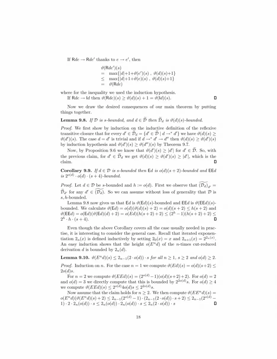
Now we draw the desired consequences of our main theorem by puttingthings together.

Lemma 9.8. If D is s-bounded, and d ∈ D then Dd is ϑ(d)(s)-bounded.

Proof. We first show by induction on the inductive definition of the reflexivetransitive closure that for every d′ ∈ Dd = {d′ ∈ D | d→∗ d′} we have ϑ(d)(s) ≥ϑ(d′)(s). The case d = d′ is trivial and if d→∗ d′ → d′′ then ϑ(d)(s) ≥ ϑ(d′)(s)by induction hypothesis and ϑ(d′)(s) ≥ ϑ(d′′)(s) by Theorem 9.7.

Now, by Proposition 9.6 we know that ϑ(d′)(s) ≥ |d′| for d′ ∈ D. So, with

the previous claim, for d′ ∈ Dd we get ϑ(d)(s) ≥ ϑ(d′)(s) ≥ |d′|, which is theclaim.

Corollary 9.9. If d ∈ D is s-bounded then Ed is o(d)(s + 2)-bounded and EEdis 2o(d) · o(d) · (s+ 4)-bounded.

Proof. Let d ∈ D be s-bounded and h := o(d). First we observe that (Dd)d′ =

Dd′ for any d′ ∈ (Dd). So we can assume without loss of generality that D iss, h-bounded.

Lemma 9.8 now gives us that Ed is ϑ(Ed)(s)-bounded and EEd is ϑ(EEd)(s)-bounded. We calculate ϑ(Ed) = o(d)(ϑ(d)(s) + 2) = o(d)(s + 2) ≤ h(s+ 2) andϑ(EEd) = o(Ed)(ϑ(Ed)(d) + 2) = o(Ed)(h(s+ 2) + 2) ≤ (2h − 1)(h(s+ 2) + 2) ≤2h · h · (s+ 4).

Even though the above Corollary covers all the case usually needed in prac-tise, it is interesting to consider the general case. Recall that iterated exponen-tiation 2n(x) is defined inductively by setting 20(x) = x and 2n+1(x) = 22n(x).An easy induction shows that the height o(End) of the n-times cut-reducedderivation d is bounded by 2n(d).

Lemma 9.10. ϑ(End)(s) ≤ 2n−1(2 · o(d)) · s for all n ≥ 1, s ≥ 2 and o(d) ≥ 2.

Proof. Induction on n. For the case n = 1 we compute ϑ(Ed)(s) = o(d)(s+2) ≤2o(d)s.

For n = 2 we compute ϑ(EEd)(s) = (2o(d)−1)(o(d)(s+2)+2). For o(d) = 2and o(d) = 3 we directly compute that this is bounded by 22o(d)s. For o(d) ≥ 4we compute ϑ(EEd)(s) ≤ 2o(d)4o(d)s ≤ 22o(d)s.

Now assume that the claim holds for n ≥ 2. We then compute ϑ(EEnd)(s) =o(End)(ϑ(End)(s) + 2) ≤ 2n−1(2

o(d) − 1) · (2n−1(2 · o(d)) · s+ 2) ≤ 2n−1(2o(d) −

1) · 2 · 2n(o(d)) · s ≤ 2n(o(d)) · 2n(o(d)) · s ≤ 2n(2 · o(d)) · s

18

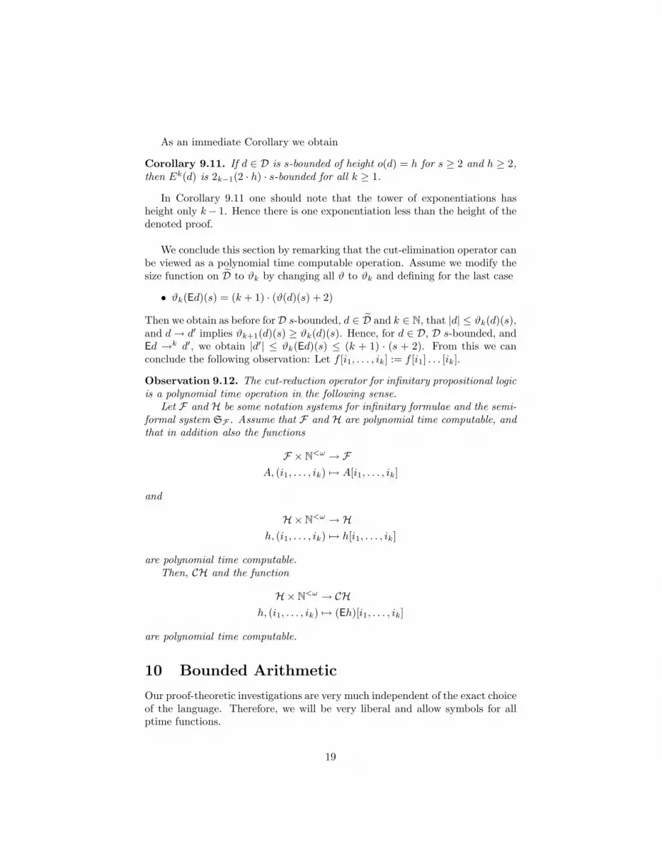
As an immediate Corollary we obtain

Corollary 9.11. If d ∈ D is s-bounded of height o(d) = h for s ≥ 2 and h ≥ 2,then Ek(d) is 2k−1(2 · h) · s-bounded for all k ≥ 1.

In Corollary 9.11 one should note that the tower of exponentiations hasheight only k− 1. Hence there is one exponentiation less than the height of thedenoted proof.

We conclude this section by remarking that the cut-elimination operator canbe viewed as a polynomial time computable operation. Assume we modify thesize function on D to ϑk by changing all ϑ to ϑk and defining for the last case

• ϑk(Ed)(s) = (k + 1) · (ϑ(d)(s) + 2)

Then we obtain as before for D s-bounded, d ∈ D and k ∈ N, that |d| ≤ ϑk(d)(s),and d→ d′ implies ϑk+1(d)(s) ≥ ϑk(d)(s). Hence, for d ∈ D, D s-bounded, andEd →k d′, we obtain |d′| ≤ ϑk(Ed)(s) ≤ (k + 1) · (s + 2). From this we canconclude the following observation: Let f [i1, . . . , ik] := f [i1] . . . [ik].

Observation 9.12. The cut-reduction operator for infinitary propositional logicis a polynomial time operation in the following sense.

Let F and H be some notation systems for infinitary formulae and the semi-formal system SF . Assume that F and H are polynomial time computable, andthat in addition also the functions

F × N<ω → F

A, (i1, . . . , ik) 7→ A[i1, . . . , ik]

and

H× N<ω → H

h, (i1, . . . , ik) 7→ h[i1, . . . , ik]

are polynomial time computable.Then, CH and the function

H× N<ω → CH

h, (i1, . . . , ik) 7→ (Eh)[i1, . . . , ik]

are polynomial time computable.

10 Bounded Arithmetic

Our proof-theoretic investigations are very much independent of the exact choiceof the language. Therefore, we will be very liberal and allow symbols for allptime functions.

19

Definition 10.1 (Language of Bounded Arithmetic). The language LBA ofBounded Arithmetic contains as non-logical symbols {=,≤} for the binary rela-tion “equality” and “less than or equal”, and a symbol for each ptime function.In particular, it includes a constant ca for a ∈ N whose interpretation in thestandard model N is cN

a = a, unary function symbols | · | and 2|·| which have theirstandard interpretation given by (|ca|)N = n and (2|ca|)N = 2n where n is thelength of the binary representation of a, and the binary function symbols minand # whose standard interpretation are minimisation and (ca # cb)

N = 2n·m

where n and m are the lengths of the binary representations of a resp. b. Wewill often write n instead of cn, and 0 for c0.

Atomic formulae are of the form s = t or s ≤ t where s and t are terms.Literals are expressions of the form A or ¬A where A is an atomic formula.Formulas are build up from literals by means of ∧ , ∨ , (∀x), (∃x). The negation¬C for a formula C is defined via de Morgan’s laws. Negation extends to setsof formulae in the usual way by applying it to their members individually.

Let C be a set of LBA-formulae (think of Σbi ), and A an LBA-formula. We

define the C-rank of A, denoted C-rk(A), by induction on the build-up of A:

• If A ∈ C ∪ ¬C, let C-rk(A) := 0.

• If A = B ∧ C or A = B ∨ C, let C-rk(A) := 1 + max{C-rk(B), C-rk(C)}.

• If A = (∀x)B or A = (∃x)B, let C-rk(A) := 1 + C-rk(B).

We will use the following standard abbreviations.

Definition 10.2 (Abbreviations). The expression A → B denotes the expres-sion ¬A ∨ B. The expression s < t denotes ¬t ≤ s. Bounded quantifiers areintroduced as follows: (∀x ≤ t)A denotes (∀x)Ax(min(x, t)), (∃x ≤ t)A denotes(∃x)Ax(min(x, t)), (∀x < t)A denotes (∀x ≤ t)(x < t → A), (∃x < t)A denotes(∃x≤ t)(x < t ∧ A), where x may not occur in t.

Definition 10.3 (Bounded Formulas). The set BFOR of bounded LBA-formulaeis the set of LBA-formulae consisting of literals and closed under ∧ , ∨ , (∀x≤t),(∃x≤ t).

We now define a restricted (also called “strict”) delineation of bounded for-mulae.

Definition 10.4. The set sΣbd is the subset of bounded LBA-formulae whose

elements are of the form

(∃x1 ≤ t1)(∀x2 ≤ t2) . . . (Qxd ≤ td)(Qxd+1 ≤ |td+1|)A(~x)

with Q and Q being of the corresponding alternating quantifier shape, and Abeing quantifier free.

Definition 10.5. As axioms we allow all disjunctions of literals, i.e., all dis-junctions A of literals such that A is true in N under any assignment. Let usdenote this set of axioms by BASIC.

20

We will base the definition of Bounded Arithmetic theories on a somewhatstronger normal form of induction. Let | · |m denote the m-fold iteration of thefunction symbol | · |.

Definition 10.6. Let Ind(A, z, t) denote the expression

Az(0) ∧ (∀z < t)(A → Az(s z)) → Az(t) .

The set Φ-LmIND consists of all expressions of the form

Ind(A, z, 2||t|m|)

with A ∈ Φ, z a variable and t an LBA-term.

This restricted form of induction implies the usual form, because the follow-ing can be proven from BASIC alone.

Ind(A(min(t, z)), z, 2|t|) → Ind(A(z), z, t)

11 Notation system for Bounded Arithmetic for-

mulae

Let FBA be the set of closed formulae in BFOR. We define the outermostconnective function on FBA by

tp(A) :=

⊤ A true literal

⊥ A false literal∧A is of the form A0 ∧ A1 or (∀x)B∨A is of the form A0 ∨ A1 or (∃x)B ,

and the sub-formula function on FBA × N by

A[n] :=

A A literal

Amin(n,1) A is of the form A0 ∧ A1 or A0 ∨ A1

Bx(n) A is of the form (∀x)B or (∃x)B .

The rank and negation functions for the notation system are those defined forLBA.

We didn’t have much choice on how to render BFOR into a notation systemfor formulae. Nevertheless, the above definition already shows that we have towork with a non-trivial intensional equality. The reason is that, even though inthe process of the propositional translation we can make sure that we only haveclosed formulae, this still is not enough; we do have other closed terms than justthe canonical ones.

21

Consider, for example, an arithmetical derivation ending in

...B(f(0))

∃x.B(x)

where f is some function symbol. In the propositional translation we have toprovide some witness i for the

∨i∃x.B(x)-inference. The “obvious” choice seems

to take i = fN(0). But this would require a derivation of (∃x.B(x))[fN(0)] =B(fN(0)). The translation of the sub-derivation, on the other hand, gives us aderivation of B(f(0)). So, in order to make this a correct inference in the propo-sitional translation, he have to consider B(f(0)) and B(fN(0)) as intensionallyequal. Note that both formulae are extensionally equal.

We will now define an intensional equality which provides the above de-scribed identification. For t a closed term its numerical value tN ∈ N is definedin the obvious way. Let →1

Ndenote the rewriting relation obtained from

{(t, tN) : t a closed term

}.

For example,(∀x)(x ≤ ⌊ 1

2 (5 · 3)⌋) →1N (∀x)(x ≤ 7) .

Let ≈N denote the reflexive, symmetric and transitive closure of →1N.

Proposition 11.1. The just defined system consisting of FBA, tp, ·[·], ¬, rkand ≈N forms a notation system for formulae in the sense of Definition 4.1.

Remark 11.2. It is an open problem what the complexity of ≈N is (assuminga usual feasible arithmetisation of syntax). However, if the depth of expressionsis restricted, and the number of function symbols representing polynomial timefunctions is also restricted to a finite subset, then the relation ≈N is polynomialtime decidable. I.e., let ≈N

k denote the restriction of ≈N to expressions of depth≤ k in which at most the first k function symbols occur. Then, for each k, therelation ≈N

k is a polynomial time predicate.

From now on, we will assume that FBA implicitly contains such a constantk without explicitly mentioning it. All formulae and terms used in FBA arethus assumed to obey the abovementioned restriction on occurrences of functionsymbols and depth. We will come back to this restriction at relevant places.The next observation already makes use of this assumption.

Observation 11.3. All relations and functions in FBA are polynomial timecomputable.

Proof. Under the just fixed convention, the relation ≈N is actually ≈Nk for some

k.

Definition 11.4. Let BA∞ denote the semiformal proof system over FBA ac-cording to Definition 5.1.

22

12 A notation system for BA∞

Definition 12.1. The finitary proof system BA⋆ is the proof system overBFOR,≈N which is given by the following set of inference symbols.

(Ax∆) if∨

∆ ∈ BASIC∆

A0 A1(∧

A0∧A1)

A0 ∧A1

Ak(∨k

A0∨A1) (k ∈ {0, 1})

A0 ∨A1

Ax(y)(∧y

(∀x)A)(∀x)A

Ax(t)(∨t

(∃x)A)(∃x)A

¬F, Fy(s y)(INDy,t

F )¬Fy(0), Fy(2|t|)

¬F, Fy(s y)(INDy,n,i

F ) (n, i ∈ N)¬Fy(n), Fy(n+ 2i)

C ¬C(CutC)∅

According to Definition 2.4, a BA⋆-quasi derivation h is equipped with func-tions Γ(h) denoting the endsequent of h, hgt(h) denoting the height of h, andsz(h) denoting the size of h.

In our finitary proof system Schutte’s ω-rule [Sch51] is replaced by ruleswith Eigenvariable conditions. Of course, the precise name of the Eigenvariabledoes not matter, as long as it is an Eigenvariable. For this reason, we thinkof the inference symbols

∧y(∀x)A, INDy,t

F , and INDy,n,iF in BA⋆-quasi derivations

as binding the variable y in the respective sub-derivations. Fortunately, wedon’t have to make this intuition precise, as we will always substitute onlyclosed (arithmetical) terms into BA⋆-derivations and therefore no renaming ofbound variables will be necessary; hence we don’t have to define what thisrenaming would mean. Note, however, that the details of Definition 12.2 ofBA⋆-derivations and Definition 12.4 of substitution become obvious with thisintuition on mind.

Definition 12.2 (Inductive definition of ~x : d). For ~x a finite list of disjointvariables and d = Id0 . . . dn−1 a BA⋆-quasi-derivation we inductively define therelation ~x : d that d is a BA⋆-derivation with free variables among ~x as follows.

• If ~x, y : h0 and I ∈ {∧y

(∀x)A, INDy,tF , INDy,n,i

F } for some A,F, t, n, i, and

FV(Γ(Ih0)) ⊂ {~x} then ~x : Ih0.

• If ~x : h0 and FV((∃x)A),FV(t) ⊆ {~x} then ~x :∨t

(∃x)Ah0.

• If ~x : h0, ~x : h1 and FV(C) ⊆ {~x} then ~x : CutCh0h1.

• If FV(∆) ⊆ {~x} then ~x : Ax∆,

• If ~x : h0, ~x : h1 and I =∧

A0∧A1with FV(A0 ∧A1) ⊂ {~x} then ~x : Ih0h1.

• If ~x : h0 and I =∨k

A0∨A1with FV(A0 ∨A1) ⊂ {~x} then ~x : Ih0.

23

A BA⋆-derivation is a BA⋆-quasi derivation h such that for some ~x it holds~x : h. We call a BA⋆-derivation h closed, if ∅ : h.

Proposition 12.3. If ~x : h then FV(Γ(h)) ⊆ {~x}. In particular FV(Γ(h)) = ∅for closed h.

Proof. Trivial induction on the inductive definition of ~x : h.

Definition 12.4. For h a BA⋆-derivation, y a variable and t a closed termof Bounded Arithmetic we define the substitution h(t/y) inductively by set-ting (Ih0 . . . hn−1)(t/y) to be I(t/y)h0(y/t) . . . hn−1(t/y) if I is not of the form∧y

(∀x)A, INDy,tF , or INDy,n,i

F with the same variable y, and Ih0 . . . hn−1 other-wise.

Substitution for inference symbols is defined by setting

Ax∆(t/y) = Ax∆(t/y)∧A0∧A1

(t/y) =∧

(A0∧A1)(t/y)

∨kA0∧A1

(t/y) =∨k

(A0∧A1)(t/y)∧z(∀x)A(t/y) =

∧z((∀x)A)(t/y)

∨t′

(∃x)A(t/y) =∨t′(t/y)

((∃x)A)(t/y)

INDz,t′

F (t/y) = INDz,t′(t/y)F (t/y) INDz,n,i

F (t/y) = INDz,n,iF (t/y)

We now show the substitution property for BA⋆-derivations. The formu-lation of Lemma 12.5 might look a bit strange with “⊆” instead of the morefamiliar equality. The reason is, that a substitution may make formulae equalwhich are not equal without the substitution.

Recalling however Definition 5.3, we note that derivations h in fact proveevery superset of Γ(h). Of course, an easy consequence of Lemma 12.5 is thatif Γ(h) ⊂ ∆ then Γ(h(t/y)) ⊂ ∆(t/y).

Lemma 12.5. Assume ~x : h and let y be a variable and t a closed term, then~x \ {y} : h(t/y) and moreover Γ(h(t/y)) ⊆ (Γ(h))(t/y).

Proof. We argue by induction on the build-up of h.In the cases where no substitution occurs (as h = I . . . with I of the form∧y

(∀x)A, INDy,tF , or INDy,n,i

F with the same variable y) both claims are trivial.Otherwise, by induction hypothesis, we know that the sub-derivations are

BA⋆-derivations with the correct set of free variables; since substitution is alsocarried out in the inference symbols, the y in the variable conditions for CutC

and∨t

(∃x)A will also disappear due to the substitution. The Eigenvariable con-

dition z 6∈ FV(Γ(h)) will follow once we have shown the second claim.For the second claim we compute by induction hypothesis

Γ((h(t/y))(ι)) = Γ((h(ι))(t/y)) ⊆ Γ((h(ι)))(t/y)

24

Hence

Γ(h(t/y)) = ∆(last(h(t/y))) ∪⋃

ι<| last(h)|

(Γ((h(t/y))(ι)) \ ≈N∆ι(last(h(t/y)))

)

i.h.⊆ ∆(last(h))(t/y) ∪

⋃

ι<| last(h)|

(Γ((h)(ι))(t/y) \ ≈N∆ι(last(h))(t/y)

)

!!!⊆

(∆(last(h)) ∪

⋃

ι<| last(h)|

(Γ((h)(ι)) \ ≈N∆ι(last(h))

))(t/y)

= Γ(h)(t/y)

This finishes the proof.

We will now define the ingredients for a notation system for BA∞, whichforms the embedding of BA⋆ into BA∞.

Let HBA be the set of closed BA⋆-derivations.For each h ∈ HBA we define the denoted last inference tp(h) as follows: Let

h = Ih0 . . . hn−1,

tp(h) :=

AxA if I = Ax∆, where A is the “least” true literal in ∆∧A0 ∧ A1

if I =∧

A0 ∧ A1∨kA0 ∨ A1

if I =∨k

A0 ∨ A1∧(∀x)A if I =

∧y(∀x)A∨tN

(∃x)A if I =∨t

(∃x)A

Rep if I = INDy,tF

Rep if I = INDy,n,0F

CutFy(n+2i) if I = INDy,n,i+1F

CutC if I = CutC

For each h ∈ HBA and j ∈ N we define the denoted sub-derivation h[j] asfollows: Let h = Ih0 . . . hn−1. If j ≥ | tp(h)| let h[j] := Ax0=0. Otherwise,assume j < | tp(h)| and define

h[j] :=

hmin(j,1) if I =∧

A0 ∧ A1

h0 if I =∨k

A0 ∨ A1

h0(j/y) if I =∧y

(∀x)A

h0 if I =∨t

(∃x)A

INDy,0,|t|N

F h0 if I = INDy,tF

h0(n/y) if I = INDy,n,0F

INDy,n,iF h0 if I = INDy,n,i+1

F and j = 0

INDy,n+2i,iF h0 if I = INDy,n,i+1

F and j = 1

hj if I = CutC

25

The denoted end-sequent function on HBA is given by Γ computed accordingto Definition 2.4. The size function |·| on HBA is given by |h| := sz(h).

To define the denoted height function we need some analysis yielding anupper bound to the log of the lengths of inductions which may occur duringthe embedding (we take the log as this bounds the height of the derivation treewhich embeds the application of induction). Let us first assume m is such anupper bound, and let us define the denoted height om(h) of h relative to m: Fora BA⋆-derivation h = Ih0 . . . hn−1 we define

om(h) :=

om(h0) + i+ 1 if I = INDy,n,iF

om(h0) +m+ 1 if I = INDy,tF

1 + supi<n om(hi) otherwise

Observe that om(h) > 0 (in particular, o(Ax∆) = 1).To fill the gap of providing a suitable upper bound function of BA⋆-derivations

we first need to fix monotone bounding terms for any term in LBA.

Bounding terms

For a term t we define a term bd(t) which represents a monotone function withthe following property: If FV(t) = {~x} then

(∀~n) t~x(~n)N ≤ bd(t)~x(~n)N

Let x0, x1, x2, . . . be a fixed list of free variables. We fix for each function symbolf of arity n a monotone bounding term Tf with FV(Tf ) ⊆ {x0, . . . , xn−1}. E.g.,assume that we have fixed for each function symbol f in our language a numbercf ∈ N such that (∀~n)|fN(~n)| ≤ max{2, |~n|}2cf

holds. We then can define

Tf := (max{2, ~x}) # . . .# (max{2, ~x})︸︷︷︸2cf times

.

As the only exception we demand that T|·| := |x0|.

Now, let t be a term. If t is a closed term, let bd(t) := tN. If t = ft1 . . . tnis not a closed term, let bd(t) := (Tf )~x(bd(t1), . . . ,bd(tn)).

Bounding terms for BA⋆-derivations

For h ∈ HBA, the bounding term bd(h) is intended to bound any variable whichoccurs during the embedding of h, and the term | ibd(h)| is intended to boundthe length of any induction which occurs during the embedding of h.

26

Let h = Ih0 . . . hn−1 be in HBA.. We define

bd(h) :=

max(bd(h0(bd(t)/y)), bd(t)) if I =∧y

(∀x≤t)A

max(bd(h0), bd(t)) if I =∨t

(∃x)A

max(bd(h0(2| bd(t)|/y)), 2|bd(t)|) if I = INDy,t

F

max(bd(h0(n+ 2i/y)), n+ 2i) if I = INDy,n,iF

max(bd(h0), . . . ,bd(hn−1)) otherwise.

ibd(h) :=

ibd(h0(bd(t)/y)) if I =∧y

(∀x≤t)A

max(ibd(h0(2| bd(t)|/y)), 2|bd(t)|) if I = INDy,t

F

max(ibd(h0(n+ 2i/y)), 2i) if I = INDy,n,iF

max(ibd(h0), . . . , ibd(hn−1)) otherwise.

Now we can define the denoted height function o(h) := o| ibd(h)|(h) for h ∈HBA.

Theorem 12.6. The just defined system consisting of HBA, tp, ·[·], Γ, o(·) and| · | forms a notation system for BA∞ in the sense of Definition 7.1.

Proof. First, we observe that o(·) satisfies the following monotonicity property:

m ≤ m′ ⇒ om(h) ≤ om′(h) . (2)

We also observe the following substitution property by inspection:

om(h(t/y)) = om(h) . (3)

We prove the following slightly more general assertion:

m ≥ | ibd(h)| & i < | tp(h)| ⇒ om(h[i]) < om(h) (4)

Then the assertion of the theorem follows using the monotonicity property (2),as ibd(h[i]) ≤ ibd(h).

The proof of (4) is by induction on the build-up of h. Let h = Ih0 . . . hn−1.First assume that h[i] = hj(t/y). The definition of om immediately shows

that in this case om(h) = 1 + supi<n om(hi). The substitution property (3)shows that om(hj(t/y)) = om(hj). Hence

om(h) > om(hj) = om(hj(y/k)) = om(h[i]) .

The remaining cases are the following ones:

If h = INDy,tF h0, then h[0] = IND

y,0,|t|F h0. As |t| ≤ | bd(t)| < | ibd(h)| ≤ m

we obtain

om(h[0]) = om(h0) + |t| + 1 < om(h0) +m+ 1 = om(h) .

If h = INDy,n,k+1F h0, then h[i] = INDy,n′,k

F h0 for some n′ Hence

om(h[i]) = om(h0) + k + 1 < om(h0) + k + 2 = om(h) .

27

Thus, assertion (4) is proven. The Theorem follows using the next Propo-sition which shows the local faithfulness property of the denoted end-sequentfunction Γ.

Proposition 12.7. Γ satisfies the local faithfulness property: Let h ∈ BA⋆,then

∆(tp(h)) ∪⋃

ι<| tp(h)|

(Γ(h[ι]) \ ≈N∆ι(tp(h)))

)⊆ ≈NΓ(h) .

Proof by induction on o(h). Let h = Ih0 . . . hn−1 ∈ HBA. We abbreviate

∗(h) := ∆(tp(h)) ∪⋃

ι<| tp(h)|

(Γ(h[ι]) \ ≈N∆ι(tp(h)))

).

Case 1. I = Ax∆: Let A be the “least” true literal in ∆, then

∗(h) = ∆(AxA) = {A} ⊆ ∆ = Γ(h)

Case 2. I =∧

C for C = A0 ∧A1: tp(h) =∧

C , h[0] = h0 and C[0] = A0, andh[ι] = h1 and C[ι] = A1 for ι > 0, hence

∗(h) = {A0 ∧ A1} ∪ (Γ(h0) \ ≈N{A0}) ∪ (Γ(h1) \ ≈N{A1})

= Γ(h)

Case 3. I =∨k

A0 ∨ A1

Case 4. I =∧y

(∀x)A: tp(h) =∧

(∀x)A, and h[ι] = h0(ι/y) and ((∀x)A)[ι] =

A(ι/x) for ι ∈ N hence

∗(h) = {(∀x)A} ∪⋃

i∈N

(Γ(h0(i/y)) \ ≈N{A(i/x)})

⊆ {(∀x)A} ∪⋃

i∈N

(Γ(h0)(i/y) \ ≈N{A(i/x)})

(1)= {(∀x)A} ∪

⋃

i∈N

(Γ(h0) \ ≈N{A})

= Γ(h)

(1): uses Eigenvariable condition.

Case 5. I =∨t

(∃x)A: tp(h) =∨tN

(∃x)A and h[0] = h0, hence

∗(h) = {(∃x)A} ∪ (Γ(h0) \ ≈N{A(tN/x)})

= {(∃x)A} ∪ (Γ(h0) \ ≈N{A(t/x)})

= Γ(h)

28

Case 6. I = INDy,tF : tp(h) = Rep and h[0] = IND

y,0,|tN|F h0, hence

∗(h) = ∅ ∪ Γ(INDy,0,|tN|F h0)

= {¬Fy(0), Fy(0 + 2|tN|)} ∪ (Γ(h0) \ ≈N{¬F, Fy(s y)})

⊆ ≈N{¬Fy(0), Fy(2|t|)} ∪ (Γ(h0) \ ≈N{¬F, Fy(s y)})

⊆ ≈NΓ(h)

Case 7. I = INDy,n,0F : tp(h) = Rep and h[0] = h0(n/y), hence

∗(h) = ∅ ∪ Γ(h0(n/y))

⊆ Γ(h0)(n/y)

(2)

⊆ ≈N{¬Fy(n), Fy(sn)} ∪ (Γ(h0) \ ≈N{¬F, Fy(s y)})

⊆ ≈N

({¬Fy(n), Fy(n+ 1)} ∪ (Γ(h0) \ ≈N{¬F, Fy(s y)})

)

= ≈NΓ(h)

(2) uses Eigenvariable condition.

Case 8. I = INDy,n,i+1F : tp(h) = CutFy(n+2i), h[0] = INDy,n,i

F h0, and h[1] =

INDy,n+2i,iF h0, hence (abbreviating Ξ := Γ(h0) \ ≈N{¬F, Fy(s y)})

∗(h) = ∅ ∪(Γ(INDy,n,i

F h0) \ ≈N{Fy(n+ 2i)})

∪(Γ(INDy,n+2i,i

F h0) \ ≈N{¬Fy(n+ 2i)})

=((

{¬Fy(n), Fy(n+ 2i)} ∪ Ξ)\ ≈N{Fy(n+ 2i)}

)

∪((

{¬Fy(n+ 2i), Fy(n+ 2i+1)} ∪ Ξ)\ ≈N{¬Fy(n+ 2i)}

)

⊆ {¬Fy(n), Fy(n+ 2i+1)} ∪ Ξ

= Γ(h)

Case 9. I = CutC : tp(h) = CutC and h[ι] = hι for ι < 2, hence

∗(h) = ∅ ∪ (Γ(h0) \ ≈N{C}) ∪ (Γ(h1) \ ≈N{¬C})

= Γ(h)

Observation 12.8. The following relations and functions are polynomial timecomputable: the finitary proof system BA⋆, the set of BA⋆-quasi derivations andthe functions h 7→ Γ(h), h 7→ hgt(h), and h 7→ sz(h) denoting the endsequent,the height and the size for a BA⋆-quasi derivation h; the bounding term t 7→bd(t) for terms t occurring in FBA and the relations bd(h) ≤ m and ibd(h) ≤ mon HBA × N; the set HBA and the functions h 7→ tp(h), h, i 7→ h[i], h 7→ Γ(h),m,h 7→ om(h) and h 7→ |h|.

29

Proof. For bounding terms we use our assumption that a fixed (finite) num-ber of function symbols and term depth is only allowed, which implies thatterms can only denote a fixed finite number of different polynomial time com-putable functions. That bd(h) ≤ m is polynomial time computable is clear asthe computation of bd(h) computes a monotone increasing sequence of valuesby successively applying one of the finitely many polynomial time computablefunctions, and once the bound m is exceeded during this process we can alreadyoutput NO.

As the function bd(h) in general may not be polynomially bounded, wecannot conclude in general that o(h) is polynomial time computable. However,the function m,h 7→ omin(| ibd(h)|,m)(h) is polynomial time computable and willbe sufficient in our applications.

13 Computational content of proofs

Let us start by describing the idea for computing witnesses using proof trees.Assume we have a BA proof of an existential formula (∃y)ϕ(y) and we want tocompute a k such that ϕ(k) is true – in case we are interested in definable func-tions, such a situation is obtained from a proof of (∀x)(∃y)ϕ(x, y) by invertingthe universal quantifier to some n ∈ N. Assume further, we have applied someproof theoretical transformations to obtain a BA∞ derivation d of (∃y)ϕ(y) withC-crk(d) ≤ C-rk(ϕ) for some set of formulae C (the choice of C depends on thelevel of definability we are interested in). Then we can define a path through d,represented by sub-derivations

d = d0, d1, d2, . . .

with

• dℓ+1 = dℓ(i) for some i ∈ | last(dℓ)|

• Γ(dℓ) = (∃y)ϕ(y),Γℓ where all formulae A ∈ Γℓ are false and satisfyC-rk(A) ≤ C-rk(ϕ).

As d is well-founded, such a path must be finite, i.e. ends with some dℓ say.In this situation we must have that last(dℓ) =

∨k(∃y)ϕ(y) and that ϕ(k) is true.

Hence we can output k.Such a path can be viewed as the canonical path to the following local search

problem: Let F be a set of possible solutions, which is a subset of BA∞ contain-ing only those d′ which satisfy that Γ(d′) ⊆ {(∃y)ϕ(y)} ∪ Γ′ where all formulaeA ∈ Γ′ are false and satisfy C-rk(A) ≤ C-rk(ϕ). Furthermore, assume d ∈ F andthat F is closed under the following neighbourhood function N : BA∞ → BA∞

which is defined by case distinction on the shape of last(d′) for d′ ∈ F :

• last(d) = AxA cannot occur as all atomic formulae in Γ(d′) are false.

30

• last(d) =∧

A0∧A1, then A0 ∧A1 must be false, hence some of A0, A1 must

be false. Let N(d) := d(0) if A0 is false, and d(1) otherwise.

• last(d) =∧

A0∨A1, then A0 ∨A1 must be false, hence both A0, A1 must be

false. Let N(d) := d(0).

• last(d) =∧

(∀x)A(x). As (∀x)A(x) is false there is some i such that A(i) is

false. Let N(d) := d(i).

• last(d) =∨k

(∃x)A(x). If (∃x)A(x) is different from (∃y)ϕ(y) then (∃x)A(x)

must be false; let N(d) := d(0). Otherwise, let N(d) = d(0) in case ϕ(k)is false, and N(d) = d in case it is true (in which case we found a truesolution to the original search problem).

• last(dℓ) = CutC . If C is false let N(d) := d(0), otherwise let N(d) := d(1).

The idea in the following will be to use proof notations from HBA to denotethis search problem. This way we will obtain characterisations of the definablefunctions of Bounded Arithmetic theories.

The level of proof theoretic reduction will be adjusted in such a way thatoccurring formulae which have to be decided fall exactly in the computationalclass under consideration. So our main concern in order for this strategy tobe meaningful is to find feasible upper bounds for the length of such reductionsequences and for the complexity of derivation notations occurring in them.

13.1 Complexity notions for BA⋆

In order to handle the complexity of BA⋆ proof notations occurring in the set ofpossible solutions, we need some notions describing key complexity propertiesof them which we will provide first.

Although tp(A) =∧

for any A starting with a ∀, and thus we can denote in-finitely many direct sub-formulae by A[n] for all n ∈ N, only finitely many carrynon-trivial information, because all quantifiers (and in particular this outermost∀) are bounded. The next definition makes this formal by assigning first to eachclosed formula in FBA, then to each inference symbol in BA∞, and finally toeach proof notation in CHBA, its range.

Definition 13.1. Let A be a formula in FBA. We define the range of A, denotedrng(A), by

rng(A) :=

0 if A a literal ,

2 if A = B ∧ C or A = B ∨ C ,

tN + 1 if A = (∀x ≤ t)B or A = (∃x ≤ t)B .

Let I be an inference symbol of BA∞. We define the range of I, denoted

31

rng(I), by

rng(I) :=

0 if I = AxA ,

1 if I =∨k

C or I = Rep ,

rng(C) if I =∧

C ,

2 if I = CutC .

For h ∈ CHBA we define

rng(h) := rng(tp(h)) .

Definition 13.2. We extend the definition of bounding terms bd(h) and ibd(h)from HBA to CHBA in the following way by induction on the build-up of h ∈CHBA:

• If h ∈ HBA then the definition of bd(h) and ibd(h) are inherited from thedefinition of bd resp. ibd(h) on HBA.

• If h = IkCh0 then

bd(h) :=

{bd(h0) if k < rng(C) ,

0 otherwise .

ibd(h) := ibd(h0)

• bd(RCh0h1) := max{bd(h0), bd(h1)}, ibd(RCh0h1) := max{ibd(h0), ibd(h1)}.

• bd(Eh0) := bd(h0), ibd(Eh0) := ibd(h0).

Lemma 13.3. Let h ∈ CHBA.

1. If j < rng(h) then bd(h[j]) ≤ bd(h) and ibd(h[j]) ≤ ibd(h).

2. If tp(h) =∨k

C then k ≤ bd(h).

Proof by induction on the build-up of h.

Definition 13.4. For h ∈ BA⋆ ∪ CHBA we define the set of decorations of h,deco(h) ∈ Pfin(BFOR), by induction on the build-up of h. Let h = Ih0 . . . hn−1.We define

deco(h) := deco(I)( ⋃

i<n

deco(hi))

where

deco(I)(S) :=

{S ∪ ∆(I) ∪ {F} if I = INDy,t

F or I = INDy,a,iF ,

S ∪ ∆(I) otherwise .

Observation 13.5. We have Γ(h) ⊆ deco(h).

Definition 13.6. Let CompHBA be the set of all h ∈ CHBA which have theproperty that all occurrences of I

kC in h satisfy k < rng(C).

32

Definition 13.7. Let Φ be a finite set of formulae in BFOR, and let K ∈ N

be a size parameter. With ΦK we denote the set of formulae which result fromformulae in Φ by substituting free variables by constants from {ci : 0 ≤ i ≤ K}.

Lemma 13.8. Let h ∈ CompHBA and Φ ∈ Pfin(BFOR) such that deco(h) ⊆ Φ,and Φ is closed under negation and taking sub-formulae. Let j,K ∈ N and y bea variable.

1. If j ≤ K and C ∈ Φ, then C[j] ∈ ΦK .

2. If j ≤ K then deco(h(j/y)) ⊆ ΦK .

3. ∆(tp(h)) ⊆ deco(h)bd(h) (subscript bd(h) needed e.g. for INDy,n,i+1F ).

4. If j < rng(h) then deco(h[j]) ⊆ Φbd(h).

Proof. For 4., consider the case that h = RCh0h1, tp(h1) =∨k

¬C and j = 0, i.e.h[0] = I

kCh0. By 3. we have ¬C ∈ Φbd(h1), hence C ∈ Φbd(h). Also k ≤ bd(h1)

by Lemma 13.3, 2. Hence, C[k] ∈ Φbd(h) by 1. Now we compute

deco(h[0]) = {C[k]} ∪ deco(h0) ⊆ Φbd(h) ∪ Φ = Φbd(h) .

Lemma 13.9. For h ∈ CHBA we have that the cardinality of Γ(h) is boundedabove by 2 · sz(h).

Proof. Let the cardinality of a set S be denoted by card(S). We observe thatcard(∆(I)) ≤ 2 for any I ∈ BA∞. Thus we can compute for h = Ih0 . . . hn−1 ∈CHBA

card(Γ(h)) ≤ card(∆(I)) +∑

i<n

card(Γ(hi)) ≤ 2 +∑

i<n

2 · sz(hi) = 2 · sz(h) .

13.2 Search problems defined by proof notations

We identify the notation system HBA for BA∞ with the abstract system ofproof notations associated with it according to Observation 8.2. For s ∈ N asize parameter we define

HsBA := {h ∈ HBA : |h| ≤ s} .

Then HsBA is an s-bounded, abstract system of proof notations, because we

observe that h ∈ HBA and h→ h′ implies |h′| ≤ |h|.Remember that h for h ∈ CHBA denotes the abstraction of h which allows us

to view CHBA as a subsystem of HBA (see Definition 8.4 and Observation 8.5).

Definition 13.10. For h ∈ CHBA we define ϑ(h)(s) := ϑ(h)(s).

33

Theorem 9.7 now reads as follows:

Corollary 13.11. If h ∈ CHsBA and h→ h′, then ϑ(h)(s) ≥ ϑ(h′)(s).

Definition 13.12. We define a local search problem L parameterised by

• a finite set of bounded formulae Φ ⊂ BFOR,

• a “complexity class” C given as a polynomial time computable set of LBA-formulae (usually C = Σb

i for some i),

• a size parameter s ∈ N,

• an initial value function h· : N → CompHsBA, where ha is presented in the

form E . . .Eh(a/x) for some BA⋆-derivation h,

• a formula (∃y)ϕ(x, y) ∈ Φ with ¬ϕ ∈ C,

such that, for a ∈ N,

• Γ(ha) = {(∃y)ϕ(a, y)},

• C-crk(ha) ≤ 1,

• o(ha) = 2|a|O(1)

,

• ϑ(ha)(s) = |a|O(1),

• deco(ha) ⊆ Φa,

in the following way:

• The set of possible solutions F (a) ∈ Pfin(CompHsBA) is given as the set of

those h ∈ CompHsBA which satisfy:

i) Γ(h) ⊆ {(∃y)ϕ(a, y)} ∪ ∆ for some ∆ ⊆ C ∪ ¬C such that all A ∈ ∆are closed and false,

ii) C-crk(h) ≤ 1,

iii) o(h) ≤ o(ha),

iv) ϑ(h)(s) ≤ ϑ(ha)(s),

v) bd(h) ≤ bd(ha) and ibd(h) ≤ ibd(ha),

vi) deco(h) ⊆ Φbd(ha);

• The initial value function is given by i(a) := ha;

• the cost function is defined as c(a, h) := o(h); and

34

• the neighbourhood function is given by

N(a, h) :=

h[j] if tp(h) =∧

C , j < rng(C) and C[j] false ,

h[0] if tp(h) =∨i

C and C 6= (∃y)ϕ(a, y)

or tp(h) =∨i

(∃y)ϕ(a,y) and ϕ(a, i) false ,

h[0] if tp(h) = CutC and C false ,

h[1] if tp(h) = CutC and C true ,

h[0] if tp(h) = Rep ,

h otherwise .

(Observe that the just defined neighbourhood function is a multi-function dueto case

∧C .)

Proof. First observe that the initial value is indeed a possible solution, i(a) =ha ∈ F (a).

Let h ∈ F (a), h′ := N(a, h). Then we show

1. h 6= h′ implies h→ h′ and o(h′) < o(h),

2. h′ ∈ F (a).

For h = h′ the assertions are obvious. So let us assume h 6= h′. Then h′ = h[j]for some j < rng(h) by construction. Hence, the first claim is obvious.

For the second claim, we consider i)–vi) of the definition of h′ ∈ F (a): ii)is clear; iii) is obvious; for iv) observe that h → h′, thus ϑ(h′)(s) ≤ ϑ(h)(s)by Corollary 13.11; for v) observe that j < rng(h) implies bd(h′) ≤ bd(h)and ibd(h′) ≤ ibd(h) by Lemma 13.3; for vi) observe that j < rng(h) im-plies deco(h′) ⊆ (Φbd(ha))bd(h) = Φbd(ha) by Lemma 13.8, 2., because bd(h) ≤bd(ha). And finally for i) we first observe that the first condition that Γ(h) \{(∃y)ϕ(a, y)} is a subset of C ∪ ¬C consisting only of closed formulae, is satis-fied, as C-crk(h) ≤ 1. For the second condition of i) let I := tp(h). We have byProposition 7.2 that

Γ(h[j]) ⊆ ≈N

(Γ(h) ∪ ∆j(I)

)

thus it is enough to show that∨

∆j(I) is false.

• I =∧

C : ∆j(I) = {C[j]} and C[j] false by construction.

• I =∨i

C : then j = 0. If C 6= (∃y)ϕ(a, y), then ∆0(I) = {C[i]}. Now Cis false by i) of h ∈ F (a), hence C[i] must be false as well. Otherwise,∆0(I) = {ϕ(a, i)}, and ϕ(a, i) false by construction.

• I = CutC : If j = 0, then ∆0(I) = {C} and C false by construction.Otherwise, j = 1, then ∆1(I) = {¬C} and ¬C false by construction.

• I = Rep: then j = 0 and ∆0(I) = ∅ and nothing is to show.

35

Proposition 13.13 (Complexity of L). F ∈ PC, i, c ∈ FP, and N ∈ FPC [wit, 1].

Proof. First observe that the functions a 7→ i(a) = ha, a 7→ bd(ha), a 7→ibd(ha), a 7→ o(ha), a 7→ ϑ(ha), and a 7→ deco(ha) are polynomial time com-putable.

Furthermore, the relations CompHsBA, C-crk(h) ≤ 1, bd(h) ≤ m, ibd(h) ≤ m

and deco(h) ⊆ Φm are polynomial time computable, and once ibd(h) ≤ m isestablished we also can compute o(h) ≤ m′ and then o(h) in polynomial time.Hence c ∈ FP

Also, the functions tp(h) and h[i] are polynomial time computable on CHBA,which shows N ∈ FPC [wit, 1].

For F ∈ PC observe that Γ(h) ⊆ deco(h) ⊆ Φbd(ha), hence condition h ∈F (a), i), is a property in PC .

Proposition 13.14 (Properties of L). 1. N(a, h) = h implies tp(h) =∨i

(∃y)ϕ(a,y)

with ϕ(a, i) true. Thus, the local search problem L defines a multi-functionby mapping a to i (this is called the computed multi-function).

2. The search problem L in general defines a search problem in PLSC, assum-ing that we turn the neighbourhood (multi-)function into a real function,which can easily be achieved by using an intermediate PLSC search prob-lem which looks for the smallest witness for the case tp(h) =

∧C . Then

N ∈ FPC.

3. Assume o(ha) = |a|O(1). Then the canonical path through L, which startsat ha and leads to a local minimum, is of polynomial length with terms ofpolynomial size, thus the computed multi-function is in FPC [wit, o(ha)].

13.3 Σbi -definable multi-functions in Si−1

2

Let i ≥ 2 and assume that Si−12 ⊢ (∀x)(∃y)ϕ(x, y) with (∃y)ϕ(x, y) ∈ Σb

i ,ϕ ∈ Πb

i−1. By partial cut-elimination we obtain some BA⋆-derivation h suchthat

• FV(h) ⊆ {x},

• Γ(h) = {(∃y)ϕ(x, y)},

• Σbi−1-crk(h) ≤ 1, and

• o(h(a/x)) = O(||a||).

We define a search problem by stating its parameters:

• Φ := deco(h) is a finite set of formulae in BFOR,

• as the “complexity class” we take C := Σbi−1,

• for the size parameter we choose s := |h|,

36

• the initial value function is given by ha := h(a/x),

• the formula is as given, (∃y)ϕ(x, y).

This defines a local search problem according to Definition 13.12, because

• Γ(ha) = Γ(h(a/x)) = Γ(h)(a/x) = {(∃y)ϕ(a, y)},

• as h ∈ HsBA we have h(a/x) ∈ Hs

BA, hence ϑ(ha)(s) = s = O(1)

• deco(ha) ⊆ Φa by Lemma 13.8, 1.

As o(ha) = O(||a||), Proposition 13.14, 3., shows that the computed multi-

function of this search problem is in FPΣbi−1 [wit, O(log n)], which coincides with

the description given by Krajıcek [Kra93].

13.4 Σbi -definable functions in Si

2

Let i > 0 and assume that Si2 ⊢ (∀x)(∃y)ϕ(x, y) with (∃y)ϕ(x, y) ∈ Σb

i , ϕ ∈Πb

i−1. By partial cut-elimination we obtain some BA⋆-derivation h such that

• FV(h) ⊆ {x},

• Γ(h) = {(∃y)ϕ(x, y)},


• o(h(a/x)) = O(||a||).





• the initial value function is given by ha := Eh(a/x),



• Γ(ha) = {(∃y)ϕ(a, y)},

• Σbi−1-crk(ha) ≤ 1,

• o(ha) = 2o(h(a/x)) − 1 = 2O(||a||) = |a|O(1),

• as h(a/x) ∈ HsBA we have

ϑ(ha)(s) = ϑ(Eh(a/x))(s)

= o(h(a/x)) · (ϑ(h(a/x))(s) + 2)

= O(||a||) · (s+ 2) = O(||a||)

37

• deco(ha) ⊆ Φa.

As o(ha) = |a|O(1), Proposition 13.14, 3., shows that the computed multi-

function of this search problem is in FPΣbi−1 [wit, nO(1)] = FPΣb

i−1 [wit].But this immediately implies that the Σb

i -definable functions of Si2 are in

FPΣbi−1 , because a witness query to (∃z < t)ψ(u, z) can be replaced by |t| many

usual (non-witness) queries to χ(a, b, u) = (∃z < t)(a ≤ z < b∧ ψ(u, z)) using adivide and conquer strategy. This characterisation coincides with the one givenby Buss [Bus86].

13.5 Σbi -definable multi-functions in Si+1

2

Let i > 0 and assume that Si+12 ⊢ (∀x)(∃y)ϕ(x, y) with (∃y)ϕ(x, y) ∈ Σb

i ,ϕ ∈ Πb

i−1. By partial cut-elimination we obtain some BA⋆-derivation h suchthat

• FV(h) ⊆ {x},

• Γ(h) = {(∃y)ϕ(x, y)},


• o(h(a/x)) = O(||a||).





• the initial value function is given by ha := EEh(a/x),



• Γ(ha) = {(∃y)ϕ(a, y)},

• Σbi−1-crk(ha) ≤ 1,

• o(ha) = 2o(Eh(a/x)) − 1 = 2|a|O(1)

,


ϑ(ha)(s) = ϑ(EEh(a/x))(s)

= o(Eh(a/x)) · (ϑ(Eh(a/x))(s) + 2)

= |a|O(1) · (O(||a||) + 2) = |a|O(1)

• deco(ha) ⊆ Φa.

By Proposition 13.14, 2., this defines a search problem in PLSΣbi−1 . This

coincides with the description given by Buss and Krajıcek [BK94].

38

13.6 Σbi+1-definable multi-functions in Σb

i+j-L2+jIND

Let i ≥ 1, j ≥ 0, and assume that Σbi+j -L

2+jIND ⊢ (∀x)(∃y)ϕ(x, y) with

(∃y)ϕ(x, y) ∈ Σbi+1, ϕ ∈ Πb

i . By partial cut-elimination we obtain some BA⋆-derivation h such that

• FV(h) ⊆ {x},

• Γ(h) = {(∃y)ϕ(x, y)},

• Σbi -crk(h) ≤ j + 1, and

• o(h(a/x)) = O(|a|3+j).



• as the “complexity class” we take C := Σbi ,


• the initial value function is given by ha := E . . .E︸︷︷︸j times

h(a/x),



• Γ(ha) = {(∃y)ϕ(a, y)},

• Σbi -crk(ha) ≤ 1,

• o(ha) ≤ 2j(o(h(a/x))) = 2j(O(|a|3+j)),


ϑ(ha)(s) = ϑ(E . . .E︸︷︷︸j×

h(a/x))(s)

= o(E . . .E︸︷︷︸(j−1)×

h(a/x)) · (ϑ((E . . .E︸︷︷︸(j−1)×

h(a/x))(s) + 2)

= 2j−1(O(|a|3+j)) · (ϑ((E . . .E︸︷︷︸(j−1)×

h(a/x))(s) + 2)

= · · · = O(|a|)

• deco(ha) ⊆ Φa by Lemma 13.8, 1.

As o(ha) = O(||a||), Proposition 13.14, 3., shows that the computed multi-

function of this search problem is in FPΣbi [wit, 2j(O(log2+j n))], which coincides

with the description given by Pollett [Pol99].

39

Acknowledgements

The authors gratefully acknowledge support by the Engineering and PhysicalSciences Research Council (EPSRC) under grant number EP/D03809X/1.

References

[AJ05] Klaus Aehlig and Felix Joachimski. Continuous normalization for thelambda-calculus and Godel’s T . Annals of Pure and Applied Logic,133(1–3):39–71, May 2005.

[AS00] Klaus Aehlig and Helmut Schwichtenberg. A syntactical analysis ofnon-size-increasing polynomial time computation. In Proceedings ofthe Fifteenth IEEE Symposium on Logic in Computer Science (LICS’00), pages 84 – 91, June 2000.

[Bec01] Arnold Beckmann. Exact bounds for lengths of reductions in typedλ-calculus. Journal of Symbolic Logic, 66(3):1277–1285, 2001.

[Bec03] Arnold Beckmann. Dynamic ordinal analysis. Arch. Math. Logic,42:303–334, 2003.

[Bec06] Arnold Beckmann. Generalised dynamic ordinals—universal measuresfor implicit computational complexity. In Logic Colloquium ’02, vol-ume 27 of Lect. Notes Log., pages 48–74. Assoc. Symbol. Logic, LaJolla, CA, 2006.

[BK94] Samuel R. Buss and Jan Krajıcek. An application of Boolean com-plexity to separation problems in bounded arithmetic. Proc. LondonMath. Soc. (3), 69(1):1–21, 1994.

[Buc91] Wilfried Buchholz. Notation systems for infinitary derivations.Archive for Mathematical Logic, 30:277–296, 1991.

[Buc97] Wilfried Buchholz. Explaining Gentzen’s consistency proof withininfinitary proof theory. In Computational logic and proof theory (Vi-enna, 1997), volume 1289 of Lecture Notes in Comput. Sci., pages4–17. Springer, Berlin, 1997.

[Bus86] Samuel R. Buss. Bounded arithmetic, volume 3 of Studies in ProofTheory. Lecture Notes. Bibliopolis, Naples, 1986.

[Bus04] Samuel R. Buss. Bounded arithmetic and constant depth Frege proofs.In Complexity of computations and proofs, volume 13 of Quad. Mat.,pages 153–174. Dept. Math., Seconda Univ. Napoli, Caserta, 2004.

[Gen35a] Gerhard Gentzen. Untersuchungen uber das logische Schließen. I.Mathematische Zeitschrift, 39:176–210, 1935.

40

[Gen35b] Gerhard Gentzen. Untersuchungen uber das logische Schließen. II.Mathematische Zeitschrift, 39:405–431, 1935.

[God58] Kurt Godel. Uber eine bisher noch nicht benutzte Erweiterung desfiniten Standpunkts. Dialectica, 12:280–287, 1958.

[KMS75] G. Kreisel, G.E. Mints, and S.G. Simpson. The use of abstract lan-guage in elementary metamathematics: Some pedagogic examples. InR. Parikh, editor, Logic Colloquium, volume 453 of Lecture Notes inMathematics, pages 38–131. Springer, 1975.

[Kra93] Jan Krajıcek. Fragments of bounded arithmetic and bounded queryclasses. Trans. Amer. Math. Soc., 338(2):587–598, 1993.

[Min78] Grigori E. Mints. Finite investigations of transfinite derivations. Jour-nal of Soviet Mathematics, 10:548–596, 1978. Translated from: Zap.Nauchn. Semin. LOMI 49 (1975). Cited after Grigori Mints. Selectedpapers in Proof Theory.Studies in Proof Theory. Bibliopolis, 1992.

[Pol99] Chris Pollett. Structure and definability in general bounded arith-metic theories. Ann. Pure Appl. Logic, 100(1-3):189–245, 1999.

[PW85] J. Paris and A. Wilkie. Counting problems in bounded arithmetic.In A. Dold and B. Eckmann, editors, Methods in Mathematical Logic(Proceedings Caracas 1983), number 1130 in Lecture Notes in Math-ematics, pages 317–340. Springer, 1985.

[Sch51] Kurt Schutte. Die unendliche Induktion in der Zahlentheorie. Math-ematische Annalen, 122:369–389, 1951.

[Tai68] William W. Tait. Normal derivability in classical logic. In J. Barwise,editor, The Syntax and Semantics of Infinitatry Languages, number 72in Lecture Notes in Mathematics, pages 204–236. Springer, 1968.

41

Documents

On the computational complexity of cut-reduction