Ann Univ FerraraDOI 10.1007/s11565-009-0079-z

On the effect of external forces on incompressible fluidmotions at large distances

Hyeong-Ohk Bae · Lorenzo Brandolese

Received: 29 April 2009 / Accepted: 25 May 2009© Università degli Studi di Ferrara 2009

Abstract We study incompressible Navier–Stokes flows in Rd with small and well

localized data and external force f . We establish pointwise estimates for large |x | of theform ct |x |−d ≤ |u(x, t)| ≤ c′

t |x |−d , where ct > 0 whenever∫ t

0

∫f (x, s) dx ds �= 0.

This sharply contrasts with the case of the Navier–Stokes equations without force,studied in Brandolese and Vigneron (J Math Pures Appl 88:64–86, 2007) where thespatial asymptotic behavior was |u(x, t)| � Ct |x |−d−1. In particular, this shows thatexternal forces with non-zero mean, no matter how small and well localized (say, com-pactly supported in space-time), increase the velocity of fluid particles at all times tand at at all points x in the far-field. As an application of our analysis on the pointwisebehavior, we deduce sharp upper and lower bounds of weighted L p-norms for strongsolutions, extending the results obtained in Bae et al. (to appear) for weak solutions,by considering here a larger (and in fact, optimal) class of weight functions.

Keywords Navier–Stokes · Asymptotic profiles · Asymptotic behavior · Far-field ·Spatial infinity · Strong solutions · Incompressible viscous flows · Decay estimates

Mathematics Subject Classification (2000) MSC 76D05 · MSC 35Q30

This research was supported by EGIDE, through the program Huber-Curien “Star” N. 16560RK.

H.-O. BaeDepartment of Mathematics, School of Natural Sciences, Ajou University,Suwon 443-749, Koreae-mail: hobae@ajou.ac.kr

L. Brandolese (B)Université de Lyon, Université Lyon 1, CNRS UMR 5208, Institut Camille Jordan,43, bd. du 11 novembre 1918, 69622 Villeurbanne Cedex, Francee-mail: brandolese@math.univ-lyon1.fr

123

Ann Univ Ferrara

1 Introduction

Let d ≥ 2 be an integer. We consider the Navier–Stokes equations in Rd , for an

incompressible fluid submitted to an external force f : Rd × R

+ → Rd :

⎧⎨

⎩

∂t u + u · ∇u = �u − ∇ p + fdiv u = 0u(x, 0) = a(x).

(1.1)

We want to investigate the effect of the external force on the large time and spatialasymptotics of the solution. In particular, we will show that even if f is small andwell localized (say, compactly supported in space-time) but with non-zero mean, thenthe velocity of the fluid particles at all times t > 0 and in all point x outside ofballs B(0, R(t)) with large radii, is considerably faster than in the case of the freeNavier–Stokes equations.

This sharply contrasts with the asymptotic properties of the solution of other semi-linear parabolic equations, where localized external forces do not affect the behaviorof the solution as |x | → ∞: only the large time behavior is influenced by the force.

The main results of the paper will be stated in Sect. 3: they include new sharppointwise estimates of the form

ct |x |−d ≤ |u(x, t)| ≤ c′t |x |−d , (1.2)

valid for 0 < t < t0 small enough and |x | ≥ R(t). Such pointwise estimates should becompared to those in the case of the Navier–Stokes equations without forcing studiedin [5], where the behavior of u is like t |x |−d−1. The constant c in (1.2) essentiallydepends on the integral of f .

Estimates (1.2) can be applied, e.g., to the case of compactly supported initial data.In such case, they describe how fast fluid particles start their motion in the far field,at the beginning of the evolution. An even more precise description of the motion offlows with localized data at large distances will be given by the following asymptoticprofile. Such profile is valid for all t > 0 such that the strong solution u is defined,and for all |x | R(t), with R(t) > 0:

u(x, t) � K(x)

t∫

0

∫f (y, s) dy ds, (1.3)

where K(x) is the matrix of the second order derivatives of the fundamental solutionof the Laplacian in R

d . As such, K j,k(x) is a homogeneous function of degree −d.See Theorem 3.1, Sect. 3, for a more precise statement.

As a consequence of our asymptotic profiles one can also recover some knownbounds on the large time behavior of L p-norms for strong solutions with very shortproofs. See, e.g., [1–3,7,8,10,11,14–17,19,20] for a small sample of recent workson this topic by different authors and related developments. Our approach is differentfrom that of these papers since it consists in deducing information on spatial norms

123

Ann Univ Ferrara

about the solution from information on their pointwise behavior. As such, it is not sowell suited for the study of weak solutions as it is for that of strong, small solutions.However, its advantage is that it allows to get sharp estimates, both from above andbelow, also in the case of L p-norms with weight like, e.g., (1+|x |)α , for a wider rangeof the parameters p and α. Namely, we will prove that, under localization assumptionson the datum and the force, and provided

∞∫

0

∫f (y, s) dy ds �= 0,

then, for 1 < p ≤ ∞, α ≥ 0 and t → ∞,

‖(1 + |x |)αu(t)‖p � ct−12 (d−α−d/p), if α + d/p < d.

The above restriction on the parameters p and α are optimal, as we will show that, forall t > 0, and 1 ≤ p < ∞,

‖(1 + |x |)αu(t)‖p = +∞ if α + d/p ≥ d.

See Theorem 3.2, Sect. 3, for more precise statements.

2 Preliminary material

The assumptions on the external force will be the following:

| f (x, t)| ≤ ε[(1 + |x |)−d−2 ∧ (1 + t)−(d+2)/2

](2.1)

‖ f ‖L1(Rd×R+) ≤ ε (2.2)

for some (small) ε > 0 and a.e. xεRd and t ≥ 0. Note that assumption (2.2) can be

interpreted as a logarithmic improvement on the decay estimate (2.1). Of course, anadditional potential force ∇Φ could also be added, affecting in this way the pressureof the fluid, but not its velocity field. On the other hand, because of condition (2.2),and due to the unboundedness of singular integrals (the Riesz transforms) in L1 and,we are not allowed to apply the Helmholtz decomposition to f . Therefore, we willnot restrict ourselves to divergence-free external forces, as it is sometimes the case inthe literature.

The above assumptions on f , as well as the smallness assumption on the datumbelow, look stringent: we simply put assumptions that allow us to provide the shortestpossible and self-contained construction of strong solutions with some decay. Indeed,our main goal will be to show that even in the case of very nicely behaved externalforces (with non-zero mean) and data, the solution will be badly behaved at infinity.More precisely, upper bounds on f and a = u(0), no matter how good, will lead tolower bounds on u(t).

123

Ann Univ Ferrara

But for the time being, we concentrate on the simpler problem of upper bounds onu, and start by establishing the following simple result.

Proposition 2.1 Assume that f satisfies (2.1), (2.2). Let also aεL1(Rd) be a diver-gence-free vector field such that, ‖a‖1 < ε and |a(x)| ≤ ε(1 + |x |)−d for a.e. x ε R

d .If ε > 0 is small enough, then there exists a unique strong solution u of theNavier–Stokes equation (NS) satisfying, for some constant C > 0, the pointwisedecay estimates

|u(x, t)| ≤ Cε[(1 + |x |)−d ∧ (1 + t)−d/2], (2.3)

and such that u(0) = a (in the sense of the a.e. and distributional convergence ast → 0). In particular, for α ≥ 0, 1 < p ≤ ∞, we have

∥∥(1 + |x |)αu(t)

∥∥

p ≤ C(1 + t)−12 (d−α− d

p ), when α + d/p < d. (2.4)

The above estimate remains true in the limit case (α, p) = (d,∞).

Remark 2.1 The Proposition above can be viewed as the limit case of a previousresult by Takahashi [18], where pointwise decay estimates of the form |u(x, t)| ≤C

[(1 + |x |)−γ ∧ (1 + t)−γ /2

]had been obtained for 0 ≤ γ < d, with a different

method and under different assumptions.There are, on the other hand, many other methods for proving sharp upper bounds

of the form

‖(1 + |x |)αu(t)‖p ≤ Ct−12 (d−α−d/p).

For example, it would be possible to adapt the arguments of [7] or [11] to the case ofnon-zero external forces. See also [1,14,19] for other different approaches for gettingdecay estimates. However, the optimal range of the parameters α and p for the validityof such estimate is not discussed in the previous papers. Our condition α + d/p < dis more general, and turns out to be optimal whenever f has non-zero mean, as wewill show in Theorem 3.2.

We denote by P be the usual Leray projector onto the solenoidal vector fields andwith et∆ the heat semigroup. The solution of Proposition 2.1 is obtained by a straight-forward fixed point argument by solving the equivalent integral formulation:

{u(t) = et∆a − ∫ t

0 e(t−s)∆P∇ · (u ⊗ u)(s) ds + ∫ t

0 e(t−s)∆P f (s) ds

div a = 0.(2.5)

Let K(x, t) be the kernel of et∆P. It is well known, and easy to check that, for all

t > 0, K(·, t) belongs to C∞(Rd) and satisfies the scaling relation

K(x, t) = t−d/2K(x/

√t, 1),

123

Ann Univ Ferrara

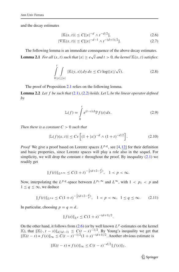
and the decay estimates

|K(x, t)| ≤ C[|x |−d ∧ t−d/2], (2.6)

|∇K(x, t)| ≤ C[|x |−d−1 ∧ t−(d+1)/2]. (2.7)

The following lemma is an immediate consequence of the above decay estimates.

Lemma 2.1 For all (x, t) such that |x | ≥ e√

t and t > 0, the kernel K(x, t) satisfies:

t∫

0

∫

|y|≤|x ||K(y, s)| dy ds ≤ Ct log(|x |/√t). (2.8)

The proof of Proposition 2.1 relies on the following lemma.

Lemma 2.2 Let f be such that (2.1), (2.2) holds. Let L be the linear operator definedby

L( f ) =t∫

0

e(t−s)∆P f (s) ds. (2.9)

Then there is a constant C > 0 such that

|L( f )(x, t)| ≤ Cε[(1 + |x |)−d ∧ (1 + t)−d/2

]. (2.10)

Proof We give a proof based on Lorentz spaces L p,q , see [4,12] for their definitionand basic properties, since Lorentz spaces will play a role also in the sequel. Forsimplicity, we will drop the constant ε throughout the proof. By inequality (2.1) wereadily get

‖ f (t)‖L p,∞ ≤ C(1 + t)−12 (d+2− d

p ), 1 < p < ∞.

Now, interpolating the L p,q -space between L p1,∞ and L∞, with 1 < p1 < p and1 ≤ q ≤ ∞, we deduce

‖ f (t)‖L p,q ≤ C(1 + t)−12 (d+2− d

p ), 1 < p < ∞, 1 ≤ q ≤ ∞. (2.11)

In particular, choosing p = q = d,

‖ f (s)‖Ld ≤ C(1 + s)−(d+1)/2.

On the other hand, it follows from (2.6) (or by well known L p-estimates on the kernelK), that ‖K(·, t − s)‖d/(d−1) ≤ C(t − s)−1/2. By Young’s inequality we get that‖K(t − s) ∗ f (s)‖∞ ≤ C(t − s)−1/2(1 + s)−(d+1)/2. Another obvious estimate is

‖K(t − s) ∗ f (s)‖∞ ≤ C(t − s)−d/2‖ f (s)‖1.

123

Ann Univ Ferrara

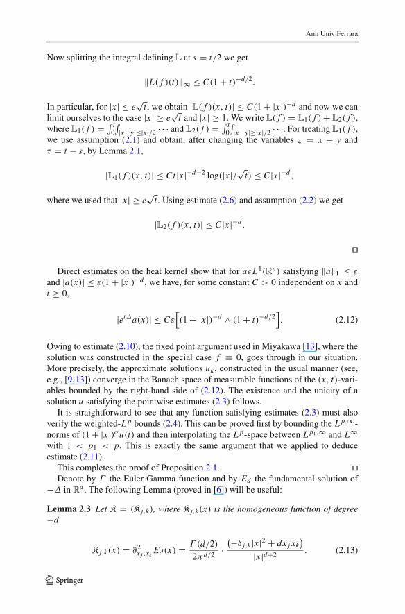
Now splitting the integral defining L at s = t/2 we get

‖L( f )(t)‖∞ ≤ C(1 + t)−d/2.

In particular, for |x | ≤ e√

t , we obtain |L( f )(x, t)| ≤ C(1 + |x |)−d and now we canlimit ourselves to the case |x | ≥ e

√t and |x | ≥ 1. We write L( f ) = L1( f ) + L2( f ),

where L1( f ) = ∫ t0

∫|x−y|≤|x |/2 · · · and L2( f ) = ∫ t

0

∫|x−y|≥|x |/2 · · ·. For treating L1( f ),

we use assumption (2.1) and obtain, after changing the variables z = x − y andτ = t − s, by Lemma 2.1,

|L1( f )(x, t)| ≤ Ct |x |−d−2 log(|x |/√t) ≤ C |x |−d ,

where we used that |x | ≥ e√

t . Using estimate (2.6) and assumption (2.2) we get

|L2( f )(x, t)| ≤ C |x |−d .

��

Direct estimates on the heat kernel show that for aεL1(Rn) satisfying ‖a‖1 ≤ ε

and |a(x)| ≤ ε(1 + |x |)−d , we have, for some constant C > 0 independent on x andt ≥ 0,

|et∆a(x)| ≤ Cε[(1 + |x |)−d ∧ (1 + t)−d/2

]. (2.12)

Owing to estimate (2.10), the fixed point argument used in Miyakawa [13], where thesolution was constructed in the special case f ≡ 0, goes through in our situation.More precisely, the approximate solutions uk , constructed in the usual manner (see,e.g., [9,13]) converge in the Banach space of measurable functions of the (x, t)-vari-ables bounded by the right-hand side of (2.12). The existence and the unicity of asolution u satisfying the pointwise estimates (2.3) follows.

It is straightforward to see that any function satisfying estimates (2.3) must alsoverify the weighted-L p bounds (2.4). This can be proved first by bounding the L p,∞-norms of (1 + |x |)αu(t) and then interpolating the L p-space between L p1,∞ and L∞with 1 < p1 < p. This is exactly the same argument that we applied to deduceestimate (2.11).

This completes the proof of Proposition 2.1. ��Denote by à the Euler Gamma function and by Ed the fundamental solution of

−∆ in Rd . The following Lemma (proved in [6]) will be useful:

Lemma 2.3 Let K = (K j,k), where K j,k(x) is the homogeneous function of degree−d

K j,k(x) = ∂2x j ,xk

Ed(x) = Γ (d/2)

2πd/2 ·(−δ j,k |x |2 + dx j xk

)

|x |d+2 . (2.13)

123

Ann Univ Ferrara

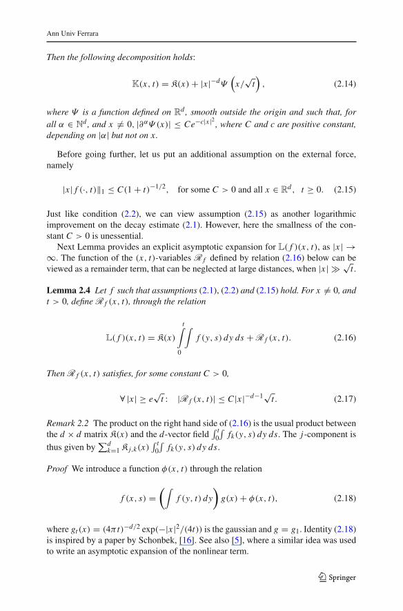
Then the following decomposition holds:

K(x, t) = K(x) + |x |−dΨ(

x/√

t)

, (2.14)

where Ψ is a function defined on Rd , smooth outside the origin and such that, for

all α ∈ Nd , and x �= 0, |∂αΨ (x)| ≤ Ce−c|x |2 , where C and c are positive constant,

depending on |α| but not on x.

Before going further, let us put an additional assumption on the external force,namely

|x | f (·, t)‖1 ≤ C(1 + t)−1/2, for some C > 0 and all x ∈ Rd , t ≥ 0. (2.15)

Just like condition (2.2), we can view assumption (2.15) as another logarithmicimprovement on the decay estimate (2.1). However, here the smallness of the con-stant C > 0 is unessential.

Next Lemma provides an explicit asymptotic expansion for L( f )(x, t), as |x | →∞. The function of the (x, t)-variables R f defined by relation (2.16) below can beviewed as a remainder term, that can be neglected at large distances, when |x | √

t .

Lemma 2.4 Let f such that assumptions (2.1), (2.2) and (2.15) hold. For x �= 0, andt > 0, define R f (x, t), through the relation

L( f )(x, t) = K(x)

t∫

0

∫f (y, s) dy ds + R f (x, t). (2.16)

Then R f (x, t) satisfies, for some constant C > 0,

∀ |x | ≥ e√

t : |R f (x, t)| ≤ C |x |−d−1√t . (2.17)

Remark 2.2 The product on the right hand side of (2.16) is the usual product betweenthe d × d matrix K(x) and the d-vector field

∫ t0

∫fk(y, s) dy ds. The j-component is

thus given by∑d

k=1 K j,k(x)∫ t

0

∫fk(y, s) dy ds.

Proof We introduce a function φ(x, t) through the relation

f (x, s) =(∫

f (y, t) dy

)

g(x) + φ(x, t), (2.18)

where gt (x) = (4π t)−d/2 exp(−|x |2/(4t)) is the gaussian and g = g1. Identity (2.18)is inspired by a paper by Schonbek, [16]. See also [5], where a similar idea was usedto write an asymptotic expansion of the nonlinear term.

123

Ann Univ Ferrara

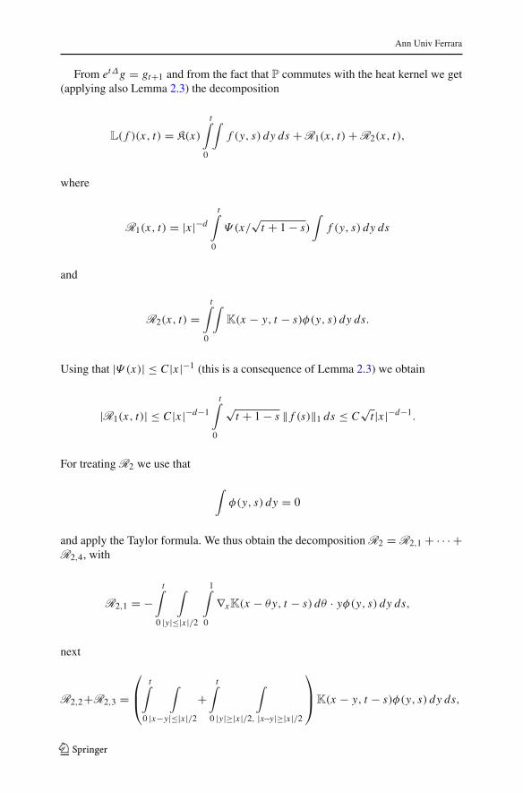
From et∆g = gt+1 and from the fact that P commutes with the heat kernel we get(applying also Lemma 2.3) the decomposition

L( f )(x, t) = K(x)

t∫

0

∫f (y, s) dy ds + R1(x, t) + R2(x, t),

where

R1(x, t) = |x |−d

t∫

0

Ψ (x/√

t + 1 − s)∫

f (y, s) dy ds

and

R2(x, t) =t∫

0

∫K(x − y, t − s)φ(y, s) dy ds.

Using that |Ψ (x)| ≤ C |x |−1 (this is a consequence of Lemma 2.3) we obtain

|R1(x, t)| ≤ C |x |−d−1

t∫

0

√t + 1 − s ‖ f (s)‖1 ds ≤ C

√t |x |−d−1.

For treating R2 we use that

∫φ(y, s) dy = 0

and apply the Taylor formula. We thus obtain the decomposition R2 = R2,1 + · · · +R2,4, with

R2,1 = −t∫

0

∫

|y|≤|x |/2

1∫

0

∇xK(x − θy, t − s) dθ · yφ(y, s) dy ds,

next

R2,2+R2,3 =⎛

⎜⎝

t∫

0

∫

|x−y|≤|x |/2

+t∫

0

∫

|y|≥|x |/2, |x−y|≥|x |/2

⎞

⎟⎠ K(x − y, t − s)φ(y, s) dy ds,

123

Ann Univ Ferrara

and

R2,4 = −t∫

0

K(x, t − s)∫

|y|≥|x |/2

φ(y, s) dy ds.

The term R2,1 is bounded using estimate (2.7) and the estimate (deduced from (2.15))

‖ |x |φ(s)‖1 ≤ C(1 + s)−1/2.

This yields |R2,1(x, t)| ≤ C |x |−d−1√t .The other three terms can be treated observing that

|φ(y, s)| ≤ C(1 + |y|)−d−2.

Then applying Lemma 2.1 we get, for |x | ≥ e√

t ,

|R2,2(x, t)| ≤ Ct |x |−d−2 log(|x |/√t) ≤ C |x |−d−1√t .

For the R2,3 term, we can observe that the integrand is bounded by C |y|−2d−2. There-fore, |R2,3(x, t)| ≤ Ct |x |−d−2 ≤ C |x |−d−1√t . The term R2,4 can be estimated inthe same way. ��

3 Main results

From the previous Lemma we now deduce the following result: it completes to thecase f �= 0 the asymptotic profile constructed in [5].

Theorem 3.1 Let f, a and u be as in Proposition 2.1. We assume that f satisfies alsocondition (2.15). Then (the notation is explained in Remark 2.2)

u(x, t) = et∆a(x) + K(x)

t∫

0

∫f (y, s) dy ds + R(x, t), (3.1)

for some function R satisfying

∀ |x | ≥ e√

t : |R(x, t)| ≤ C |x |−d−1√t, (3.2)

where C > 0 is a constant independent on x and t.

Remark 3.1 This theorem essentially states that if t > 0 is fixed and∫ t

0

∫f (y, s)

dy ds �= 0, then

u(x, t) � et∆a(x) + K(x)

t∫

0

∫f (y, s) dy ds as |x | → ∞.

123

Ann Univ Ferrara

Proof Owing to our previous Lemma, the only thing that remains to do is to write uthrough Duhamel formula (2.5) and show that

B(u, u) ≡t∫

0

e(t−s)�P∇ · (u ⊗ u)(s) ds

can be bounded by C |x |−d−1√t . In fact, a stronger estimate will be proved. Note thatthe convolution kernel F(x, t) of et∆

P∇ satisfies to the same decay estimates of ∇K

(see (2.7)). Therefore, after writing

B(u, u)(x, t) =t∫

0

∫F(x − y, t − s)(u ⊗ u)(y, s) dy ds,

then splitting the spatial integral into |y| ≤ |x |/2 and |y| ≥ |x |/2, and using that‖F(·, t − s)‖1 = c(t − s)−1/2, we get

|B(u, u)|(x, t) ≤ C |x |−d−1

t∫

0

‖u‖22 ds + (1 + |x |)−2d√

t .

When d ≥ 3, by estimate (2.4) with α = 0 and p = 2, we get∫ t

0 ‖u(s)‖22 ds ≤ C(1∧t),

which is enough to conclude. When d = 2, we have only∫ t

0 ‖u(s)‖22 ds ≤ C log(1+t).

(such facts on the L2-norm on u also follow from Schonbek’s results [15,16]). Thisyields in particular the required bound

|B(u, u)|(x, t) ≤ C√

t |x |−d−1 .

��

Remark 3.2 The asymptotic profile (3.1) leads us to study the homogeneous vectorfields of the form:

m(x) = K(x)c, c = (c1, . . . , cd).

Notice that m has a zero in Rd\{0} if and only if c = 0. Indeed, we can limit ourselves

to the points ω ∈ Sd−1 and recalling (2.13) we see that m vanishes at the point ω if

and only if

dω jω · c = c j , for j = 1, . . . , d.

123

Ann Univ Ferrara

Multiplying scalarly with ω we get (d − 1)ω · c = 0 for all ω ∈ Sd−1. As d ≥ 2, we

obtain c = 0. Applying this observation to our situation we get

infx �=0

|x |d∣∣∣∣∣∣K(x)

t∫

0

∫f (y, s) dy ds

∣∣∣∣∣∣> 0

for all t > 0 such that∫ t

0

∫f (y, s) dy ds �= 0.

A first interesting consequence of Theorem 3.1 is the following:

Corollary 3.1.1 1. Let a, f and u as in Theorem 3.1. We additionally assumethat a = u(0) satifies a(x) = o(|x |−d) as |x | → ∞. Fix t > 0 such that∫ t

0

∫f (y, s) dy ds �= 0. Then for some locally bounded function R(t) > 0 (R(t)

can blow up for t → ∞ or t → 0) and all |x | ≥ R(t), we have

ct |x |−d ≤ |u(x, t)| ≤ c′t |x |−d (3.3)

for some constant ct , c′t > 0 independent of x.

2. (Short time behavior of the flow) If in addition f εC(R+, L1(Rd)) and f0 =f (·, 0) is such that

∫f0(y) dy �= 0, then the behavior of u at the beginning of the

evolution can be described in the following way: there exists a time t0 > 0 suchthat for all 0 < t < t0 and all |x | ≥ R(t)

ct |x |−d ≤ |u(x, t)| ≤ c′t |x |−d ,

for some constants c, c′ > 0 independent of x and t.

Proof Let

m(x, t) ≡ K(x)

t∫

0

∫f (y, s) dy ds.

We apply the asymptotic expansion (3.1) for u and study each term in this expres-sion. By the non-zero mean condition on f and Remark 3.2, 3|m(x, t)| can be boundedfrom above and from below as in (3.3), for some 0 < ct < c′

t . Estimate (3.2) showsthat |R(x, t)| ≤ ct |x |−d provided |x | ≥ R(t) and R(t) > 0 is taken sufficiently large.

On the other hand, the bound |gt (x − y)| ≤ C |x − y|−d−1√t and ‖gt‖1 = 1 forthe heat kernel lead to

|et∆a(x)| ≤ C∫

|y|≤|x |/2

√t |x − y|−d−1|a(y)| dy +

∫

|y|≥|x |/2gt (x − y)|a(y)| dy

≤ C |x |−d−1√t‖a‖1 + ess sup|y|≥|x |/2|a(y)| (3.4)

and since |a(y)| = o(|y|−d) as |y| → ∞, this expression is also bounded by ct |x |−d

for |x | ≥ R(t) and a sufficiently large R(t).

123

Ann Univ Ferrara

In conclusion the first and third terms in expansion (3.1) can be absorbed by m(x, t).The first conclusion of the corollary then follows. The second conclusion is nowimmediate, because for t > 0 small enough and |x | ≥ R(t) large enough, one can findtwo constants α, β > 0 such that

αt |x |−d ≤ |m(x, t)| ≤ βt |x |−d

(the condition∫

f0(y) dy �= 0 is needed only for the lower bound). ��Remark 3.3 The result for the free Navier–Stokes equation ( f ≡ 0) is different (see[5]): instead of (3.3) one in general obtains estimates of the form

ct |x |−d−1 ≤ |u(x, t)| ≤ c′t |x |−d−1.

Therefore, an external force, even if small and compactly supported in space-time, hasthe effect of increasing the velocity of the fluid particles at all points at large distances.

We obtain, as another consequence of Theorem 3.1, the following result for thelarge time behavior.

Theorem 3.2 Let a, f and u as in Theorem 3.1. We additionally assume that a = u(0)

satisfies a(x) = o(|x |−d) as |x | → ∞ and that

∞∫

0

∫f (y, s) dy ds �= 0.

Then, for α ≥ 0, 1 < p < ∞, for some t0 > 0, some constants c, c′ > 0 and allt > t0 we have,

ct−12 (d−α− d

p ) ≤ ∥∥(1 + |x |)αu(t)

∥∥

p ≤ c′t−12 (d−α− d

p ), when α + d/p < d. (3.5)

The above inequalities remain true in the limit case (α, p) = (d,∞).On the other hand,

∥∥(1 + |x |)αu(t)

∥∥

p = +∞ when α + d/p ≥ d, (3.6)

and the above equality remains true in the limit cases p = 1 or (α > d and p = ∞).

Proof The upper bound in (3.5) has been already proved in Proposition 2.1. The proofmakes use of an argument used before in [5]. By our assumption on f and Remark 3.2,the homogeneous function

m(x) ≡ K(x)

∞∫

0

∫f (y, s) dy ds

123

Ann Univ Ferrara

does not vanish. Therefore, for some c0 > 0, we obtain |m(x)| ≥ c0|x |−d . Let usapply the profile (3.1), writing the second term on the right hand side as m(x) −K(x)

∫ ∞t

∫f (y, s) dy ds. We get for a sufficiently large M > 0, all t > M and all

|x | ≥ M√

t ,

|u(x, t) − et∆a| ≥ |m(x)| − C |x |−d−1√t − c02 |x |−d ≥ c0

3 |x |−d .

On the other hand the computation (3.4) guarantees that we can bound, for |x | ≥ M√

tand t > M, |et∆a(x)| ≤ c0

12 |x |−d . We thus get

|u(x, t)| ≥ c04 |x |−d , for all |x | ≥ M

√t, t > M . (3.7)

Let 1 < p ≤ ∞. Multiplying this inequality by the weight (1+|x |)αp, then integratingwith respect to x on the set |x | ≥ M

√t , we immediately deduce

∥∥(1 + |x |)αu(x, t)

∥∥

p ≥ ct−12 (d−α− d

p )

for some c > 0 and all t > M . In the same way, inequality (3.7) also implies the lowerbound (3.5) in the limit case p = ∞ and conclusion (3.6). The upper bounds for uobtained in Proposition 2.1 complete the proof. ��

The lower bounds obtained in (3.5) are invariant under the time translation t →t + t∗, but the hypothesis made on f,

∫ ∞0

∫f (y, s) dy ds �= 0, is not. The explanation

is that the conditions on the datum, a(x) = o(|x |−d) as |x | → ∞, and a ∈ L1(Rd), ingeneral, are not conserved at later times. In fact, according to (3.1), one has |u(x, t∗)| =o(|x |−d) as |x | → ∞ if and only if

∫ t∗0

∫f (y, s) dy ds = 0.

We did not treat the case of external forces with vanishing integrals. In that case,the principal term in the asymptotic expansion (2.16) of u as |x | → ∞ disappears.A similar method, however, can be used to write the next term in the asymptoticswhich equals

∇K(x) :t∫

0

∫y ⊗ f (y, s) dy ds

(more explicitly∑

h,k ∂hK j,k(x)∫ t

0

∫yh fk(y, s) dy ds, for the j-component, j =

1, . . . , d). For this we need to put more stringent assumptions on the decay of f :the spatial decay must be increased of a factor (1 + |x |)−1 and the time decay by afactor (1 + t)−1/2. Assumptions (2.2)–(2.15) should also be sharpened accordingly.For well localized initial data a(x), then one would deduce, bounds of the form

ct |x |−d−1 ≤ |u(x, t)| ≤ c′t |x |−d−1

and

‖(1 + |x |)αu(t)‖p � ct−12 (d+1−α−d/p), for α + d/p < d + 1.

123

Ann Univ Ferrara

However, as for the free Navier–Stokes equations (see [5]), suitable additional non-symmetry conditions on the flow and on the matrix

∫ t0

∫y ⊗ f (y, s) dy ds should be

added for the validity of the lower bounds.

References

1. Amrouche, C., Girault, V., Schonbek, M.E., Schonbek, T.P.: Pointwise decay of solutions and of higherderivatives to Navier–Stokes equations. SIAM J. Math. Anal. 31(4), 740–753 (2000)

2. Bae, H.-O., Brandolese, L., Jin, B.J.: Asymptotic behavior for the Navier–Stokes equations with non-zero external forces. Nonlinear analysis, doi:10.1016/j.na.2008.10.074 (to appear)

3. Bae, H.-O., Jin, B.J.: Upper and lower bounds of temporal and spatial decays for the Navier–Stokesequations. J. Diff. Eq 209, 365–391 (2006)

4. Bergh, J., Löfsrtom, J.: Interpolation Spaces, an Introduction. Springer, Heidelberg (1976)5. Brandolese, L., Vigneron, F.: New asymptotic profiles of nonstationnary solutions of the Navier–Stokes

system. J. Math. Pures Appl. 88, 64–86 (2007)6. Brandolese, L.: Fine properties of self-similar solutions of the Navier–Stokes equations. Arch. Rational

Mech. Anal. 192(3), 375–401 (2009)7. Choe, H.J., Jin, B.J.: Weighted estimates of the asymptotic profiles of the Navier–Stokes flow in R

n .J. Math. Anal. Appl. 344(1), 353–366 (2008)

8. He, C., Xin, Z.: On the decay properties of solutions to the nonstationary Navier–Stokes equations inR

3. Proc. Roy. Edinbourgh Soc. Sect. A. 131(3), 597–619 (2001)9. Kato, T.: Strong L p-solutions of the Navier–Stokes equations in R

m , with applications to weak solu-tions. Math. Z 187, 471–480 (1984)

10. Kukavica, I., Torres, J.J.: Weighted bounds for velocity and vorticity for the Navier–Stokes equa-tions. Nonlinearity 19, 293–303 (2006)

11. Kukavica, I., Torres, J.J.: Weighted L p decay for solutions of the Navier–Stokes equations. Comm.Part. Diff. Eq. 32, 819–831 (2007)

12. Lemarié-Rieusset, P.G.: Recent developments in the Navier–Stokes problem. Chapman & Hall, CRCPress, Boca Raton (2002)

13. Miyakawa, T.: On space time decay properties of nonstationary incompressible Navier–Stokes flowsin R

n . Funkcial. Ekvac. 32(2), 541–557 (2000)14. Oliver, M., Titi, E.: Remark on the rate of decay of higher order derivatives for solutions to the

Navier–Stokes equations in Rn . J. Funct. Anal. 172, 1–18 (2000)

15. Schonbek, M.E.: L2 decay for weak solutions of the Navier–Stokes equations. Arch. Rat. Mech. Anal.88, 209–222 (1985)

16. Schonbek, M.E.: Lower bounds of rates of decay for solutions to the Navier–Stokes equations. J. Amer.Math. Soc. 4(3), 423–449 (1991)

17. Skalák, Z.: Asymptotic decay of higher-order norms of solutions to the Navier–Stokes equations inR

3. Preprint (2009), http://mat.fsv.cvut.cz/nales/preprints/18. Takahashi, S.: A weighted equation approach to decay rate estimates for the Navier–Stokes equa-

tions. Nonlinear Anal. 37, 751–789 (1999)19. Zhang Qi, S.: Global solutions of the Navier–Stokes equations with large L2 norms in a new function

space. Adv. Diff. Eq. 9(5–6), 587–624 (2004)20. Zhou, Y.: A remark on the decay of solutions to the 3-D Navier–Stokes equations. Math. Meth. Appl.

Sci. 30, 1223–1229 (2007)

123