On the mechanism of interannual variability of the Irminger Water in the Labrador Sea

On the mechanism of interannual variability of the IrmingerWater in the Labrador Sea

J. Zhu1 and E. Demirov1

Received 30 July 2009; revised 8 October 2010; accepted 2 December 2010; published 8 March 2011.

[1] The mechanism of variability of the North Atlantic subpolar gyre (SPG) and itsrelation to the North Atlantic Oscillation (NAO) is investigated using an ocean generalcirculation model. In this study we conducted three model experiments. The first two wereforced with idealized positive (NAO+) and negative (NAO−) NAO‐like forcing, includingvariations at decadal time scales. The third experiment was forced with the NationalCenters for Environmental Prediction and National Center for Atmospheric Research(NCEP/NCAR) reanalysis. The decadal variability of the volume transport, the sea surfacetemperature in the North Atlantic Current (SSTA1), and the Irminger Water temperature(IWT) in the NAO− experiment have 2–3 times smaller magnitude than in the NAO+

experiment. The decadal variations in the strength of circulation in the NAO+ experimentcovaries negatively with SSTA1 and IWT anomalies. A similar covariability of theseparameters is not found in the NAO− simulations. The results from the model experimentforced with the NCEP/NCAR reanalysis from 1958 to 2005 show a shift in the subpolarocean response to the atmospheric variability in the early 1980s. The amplitude ofquasi‐decadal variability of the IWT and SSTA1 and their correlation are high after 1980(r = 0.79) and weaker in the period between 1958 and 1980 (r = 0.1). The IWT after1980 is well correlated (r = 0.67) to the subpolar gyre transport index (SPGI, defined as theminimum value of the annual mean anomaly of the model barotropic stream function).This correlation is weaker and negative (r = −0.09) in the period from 1958 to 1980. Weexplain this shift in the covariability of the SSTA1, IWT, and SPGI with the antisymmetricresponse of the SPG to atmospheric variations at decadal time scale under positive andnegative NAO index. The NAO sign changed in the early 1980s from predominantlynegative to positive phase. In the 1980s and 1990s the model SPGI variability followsclosely the decadal variations of the NAO index with a delay of about 3 years. Similarcovariability between the SPGI and the NAO and related negative covariance of SSTA1and IWT with the SPGI are not observed in the model simulations of the period from1958 to 1980.

Citation: Zhu, J., and E. Demirov (2011), On the mechanism of interannual variability of the Irminger Water in the LabradorSea, J. Geophys. Res., 116, C03014, doi:10.1029/2009JC005677.

1. Introduction

[2] Cyclonic circulation in the subpolar North Atlantic(Figure 1) is an important contributor to the global oceanwater and heat transport. The observed cyclonic volumetransport in the Labrador Sea is 40–50 Sv, which consists of30–38 Sv “throughput” in the subpolar gyre (SPG) and 10–14 Sv in the local recirculation [Pickart et al., 2002]. Thedeep component of this flow feeds the Meridional Over-turning Circulation (MOC). The SPG is bounded to the eastby the warm and salty North Atlantic Current (NAC)(Figure 1). In the subpolar area, the surface NAC water is

cooled through the heat exchange with the atmosphere and aportion of it penetrates into the subsurface cyclonic flow.This so‐called Irminger water (IW) is observed as a saltyand warm water mass below 150 m depth which influencesthe stratification and intensity of the vertical mixing in theSPG. Myers et al. [2007] found that the Labrador Seawater(LSW) formation is correlated (r = 0.51) to the IW transportat Cape Farewell with a lag of 1 year.[3] The temperature of the NAC surface water in area A1

(see Figure 1) increased by 1°C between late 1980s and1990s. Marsh et al. [2008] explained this change by theanomalous convergence of ocean heat transport associatedwith the overturning and horizontal circulation. The Irmin-ger Water temperature (IWT) in the Labrador Sea during thelate 1990s was warmer than usual [Myers et al., 2007].Holland et al. [2008] suggested that the related increase ofthe subsurface ocean temperature along the west coast of

1Department of Physics and Physical Oceanography, MemorialUniversity of Newfoundland, St. John’s, Newfoundland, Canada.

Copyright 2011 by the American Geophysical Union.0148‐0227/11/2009JC005677

JOURNAL OF GEOPHYSICAL RESEARCH, VOL. 116, C03014, doi:10.1029/2009JC005677, 2011

C03014 1 of 15

http://dx.doi.org/10.1029/2009JC005677

Greenland was the most likely cause for the sudden switchof Jakobshavn Isbrae from slow thickening to rapid thinningin 1997. Holland et al. [2008] also explained the warming ofthe IWT with the weakening of the SPG at the end of 1990s[Häkkinen and Rhines, 2004] and related westward move-ment of the polar frontal system [Hátún et al., 2005]. Theweakening of the SPG in the 1990s was linked to anincrease in the volume of the NAC surface water mass andrecord high salinities in the Atlantic inflow to the NordicSeas [Hátún et al., 2005]. The ocean model simulations ofBöning et al. [2006] demonstrated that the decay of thecirculation and related variability of the SPG in the late1990s was part of long‐term decadal variability of the SPG.[4] The mechanism of the SPG interannual variability in

the 1980s and 1990s has received considerable attention.Among other mechanisms, a number of studies [see Hurrell,1995; Visbeck et al., 2003; Lohmann et al., 2009] havelinked the SPG variability with the North Atlantic Oscilla-tion (NAO). Positive (negative) NAO is associated withstronger (weaker) than normal winds and cold (warm)winters in the subpolar North Atlantic. Lohmann et al.[2009] demonstrated that the SPG response is asymmetricto steady NAO‐like forcing. In the positive NAO case theSPG circulation strengthens during the first 10 years andthen it warms and weakens. In the simulations with negativeNAO forcing, the tendency in the strength of SPG circula-tion shows a persistent weakening and does not involve asign reversal. Lohmann et al. [2009] related the asymmetricSPG response to the sign of persistent NAO‐like forcing tothe nonlinearity in the North Atlantic circulation.[5] The time series of the NAO index in recent years [see

Greatbatch, 2000] has revealed a period of low values fromthe early 1950s to the early 1970s, relatively high values in

the early part of last century, and high values in the last 25–30 years, during which time the index shows also a strongdecadal variability. The NAO variations at decadal timescale had a strong impact [see Greatbatch, 2000] on thesubpolar atmosphere in the 1980s and 1990s. The winters ofthe late 1980s and early 1990s were cold with strong surfacewinds while the winters of late 1990s were anomalouslywarm. The related variations in the surface forcing had animpact on the deep convection and MOC causing the largestvariations in the properties of the LSW observed in the past60 years [Yashayaev, 2007].[6] The aim of the present work is to extend the study of

Lohmann et al. [2009] and to explore the response of the SPGto the decadal variability under positive and negative NAO‐like forcing. More specifically, here we address two questions.[7] 1. How does the asymmetric nature of the relation

between the SPG and NAO‐like forcing impact the responseof the SPG to the quasi‐decadal variations in the NAO?[8] 2. What is the impact of the atmospheric decadal

variability on the SPG in the late 1990s?[9] The article is organized as follows: section 2 describes

the model setup, section 3 discusses the model response toidealized positive and negative NAO‐like forcing, section 4presents results from model simulations of the North Atlanticforced with 1948–2005 National Centers for EnvironmentalPrediction and National Center for Atmospheric Research(NCEP/NCAR) reanalysis. Section 5 offers conclusions.

2. The Model

[10] The ocean model is the Nucleus for EuropeanModels of the Ocean (NEMO) model [Madec, 2008]. It is az coordinate, primitive equation, free surface ocean model

Figure 1. Map of the subpolar North Atlantic. The isobaths are 700, 2000, 3000, 3500, and 6000 m (lightcontours). Arrows depict schematically the surface current system (NAC, North Atlantic Current; EGC, EastGreenland Current; WGC,West Greenland Current; LC, Labrador Current; IC, Irminger Current; BC, BaffinIsland Current). The blue line defines the borders of area A1 used in calculation of SSTA1.

ZHU AND DEMIROV: MECHANISM OF IRMINGER WATER VARIABILITY C03014C03014

2 of 15

coupled with the multilayered sea ice LIM2 model [Fichefetand Morales Maqueda, 1997]. The domain covers theNorth Atlantic from 7°N to 67°N, with horizontal resolutionof 1

4° in longitude and 14° cos� in latitude �, and 46 vertical

levels. The model is forced with NCEP/NCAR reanalysisdata [Kalnay et al., 1996] from 1948 to 2005. The openboundary conditions (OBC) are imposed on the northernand southern boundaries from the Simple Ocean DataAssimilation (SODA) data set [Carton et al., 2005]. Themodel is initialized from a 30 year run forced with NCEPmonthly mean surface atmospheric fields. A spectralnudging scheme [Thompson et al., 2006] is applied toreduce model bias and drift on the climatological time scale.The model temperature and salinity are nudged toward theobserved climatology with a prescribed frequency–wavenumber band and is not constrained outside of this interval.In the following experiments, the nudging scheme is appliedto the surface 30 m layer and in the layer deeper than 560 m.In this way the IW properties and their interannual vari-ability are not affected directly by the spectral nudging.

[11] In this article we present results from three modelexperiments. The first two model runs are forced with ide-alized NAO‐like (NAO+ and NAO−) surface fluxes. Theatmospheric forcing in the third model experiment is from the6 h NCEP/NCAR reanalysis. The first 10 years of NAO+ andNAO− simulations are performed with forcing calculated asdaily composites of NCEP/NCAR atmospheric fields foryears of positive and negative NAO correspondingly. In thepositive NAO case these years are 1983, 1989, 1990, 1992,1994, 1995, 2000 and for the negative NAO the years are1963, 1964, 1965, 1969, 1977, 1979 and 1996. Starting fromthe 11th year of NAO+ and NAO− simulations, the forcingincludes a decadal variability. The near surface atmosphericparameters are calculated as sum of monthly mean plus 6 hvariability. The monthly mean fields are computed usingmonthly composites for years of positive, negative and neu-tral NAO. The years of neutral NAO are 1972, 1978, 1980,1982, 1987, 1988. The monthly forcing every 10th year in theNAO+ run, i.e., 10th year, 20th, 30th years, etc., is set equal tothe positive NAO fields. The monthly mean forcing in years

Figure 2. The SPGI (blue solid curve), the surface temperature averaged over area A1 (red dottedcurve), and the subsurface temperature off the west Greenland coast (a) from the positive NAO runand (b) from the negative NAO run (red dashed curve, defined as the temperature at 483 m averaged56°W onshore along 65°N). Note that the subsurface temperature anomalies (red dashed curve) have beenmultiplied by a factor of 2.


3 of 15

15th, 25th, 35th, etc., is equal to the neutral NAO fields. Inbetween, the monthly forcing evolves smoothly from thepositive NAO case to the neutral NAO case and then back tothe positive NAO case within every decade. The 6 h devia-tions from the monthly mean are from selected NAO+ andNAOn years (and calculated with respect to monthly means ofthe individual year). The atmospheric forcing is calculatedsimilarly for the NAO− run.

3. Response of the SPG to Positive and NegativeNAO Forcing

[12] Figure 2 shows the variability of the subpolar gyretransport index (SPGI), sea surface temperature (SST) in theNorth Atlantic Current (SSTA1), and the IWT in the NAO+

and NAO− simulations. The anomalies are calculated withrespect to the mean of the run forced with 1948–2005NCEP/NCAR reanalysis. In both simulations, the NAO+

and NAO−, the SPGI, SSTA1 and IWT reach equilibriumafter the first 5 years of simulations. Figure 2 shows thewell known [see Lohmann et al., 2009] property ofstrengthening of the SPG and cooling of IWT in the NAO+

run and weakening of SPGI and warming of IWT in theNAO− simulations. In years of positive NAO the wintersare colder and the winds are stronger than normal overthe subpolar ocean. The intensified winter convection inthese years results in stronger than usual intensity of theprocesses of deep water formation and spreading of coldsurface and intermediate water masses. The horizontal gra-dients in the density doming structure in the SPG strengthenand the SPG circulation intensifies. The change of the cir-culation of the SPG under positive NAO is spatially inho-mogeneous (see Figure 3). The intensification of the SPG isstrongest in the areas along the west coast of Greenland,northern Labrador Sea and in eastern part of the SPG(Figure 3c). These are also the areas of largest difference ofthe (SST (Figure 4) and temperature at intermediate depths(Figure 5c) in the NAO+ and NAO− experiments. Theintermediate waters the SPG are warmer in the NAO−

experiment by about 0.5°C–1.5°C (Figure 5). This increaseof the temperature in the SPG under negative NAO−

forcing (Figures 5a and 5b) is related to the increasing ofthe volume of the IW. The difference of the IWT in theNAO+ and NAO− runs have large magnitudes of about1.5°C in the eastern part of the SPG and in northern Lab-rador Sea.[13] The strongest intensification of the SPG transport in

the NAO+ simulations (Figure 3c) is about 8 Sv and ispresent a relatively narrow area along the east coast ofGreenland. The mechanism of intensification of the cyclonicflow in this area is related to the effect of the bottomtopography on the SPG boundary current. The bottompressure torque [Mellor et al., 1982; Greatbatch et al., 1991]is calculated as

BPT ¼ � J pB;Hð Þ�0 f0

where pB is the bottom pressure, H is bottom depth, r0 is meanocean density and f0 is the Coriolis parameter. The bottompressure torque has strongest impact on the flow along thewest coast of Greenland and off the coast of Labrador (see

Figures 6a and 6b). Under positive NAO, the bottom pressuretorque effect increases by up to 25% off the west coast ofGreenland. This change is primarily driven by the intensifiedwind stress and leads to local intensification of circulation.[14] After the 10th year of simulation, the surface forcing

in the two model experiments, NAO+ and NAO−, includesvariations at decadal time scale (see section 2). The analysisof the time evolution of the model parameters (not shownhere) suggests that the model solution adjusts to the variablesurface wind and buoyancy forcing through propagation oftopographic Rossby waves which travel along the coast ofthe subpolar ocean for about 2–3 years. This time scale isconsistent with findings of Eden and Willebrand [2001],Brauch and Gerdes [2005], and Lohmann et al. [2009] thatthe SPG responds with a delay of 2–3 years to the changesin the surface forcing.

Figure 3. The barotropic stream function averaged overyears 6–10 in (a) the positive NAO run and (b) the negativeNAO run. (c) The difference between Figures 3a and 3b.Contour interval is 5 Sv in Figures 3a and 3b and 1 Sv inFigure 3c.


4 of 15

[15] The SPGI, SSTA1 and IWT from the 11th to 23rdyears of simulations are shown in Figure 7. Like in thesimulations with steady NAO‐like forcing, the ITW andSSTA1 anomalies are mostly positive in the NAO− andnegative in the NAO+ simulations. The two parameterscorrelate well with r = 0.67 in the NAO+ run and r = 0.62 inthe NAO− experiment. However, the amplitude of variationsof the ITW is two to three times higher in the NAO+

experiment. In this run, the ITW variability follows thevariations of the NAO index. The maximums and mini-mums in the IWT in NAO+ experiment (see Figure 7a)occur 1–2 years after the time of neutral NAO index (15thyear) and maximum NAO index (22th year), respectively.The IWT variations in the NAO− experiment are less con-sistent with the variability of the NAO index (Figure 7b) anddoes not show a clear connection with the changes of NAOfrom neutral phase in the 15th year to negative phase in 20thyear. The intensity of SPG circulation is stronger thannormal in the NAO+ run (blue curve in Figure 7a) andweaker than normal in the NAO− simulations (Figure 7b).More detailed information about changes in the volumetransport related to the NAO variations is given by thespatial distribution of the stream function for the two runsin Figures 8 and 9.[16] Figure 8 shows the decadal mean barotropic stream

function over years from 13 to 23 (Figure 8a) and the dif-ference of the volume transport in years 17 and 22 (Figure 8b)in the NAO+ run. The same characteristics but for theNAO− experiment are shown in Figures 9a and 9b. Thedecadal mean volume transport in both experiments aresimilar to the results from the first 10 years of the NAO+ andNAO− simulations forced with NAO‐like forcing withoutinterannual and decadal variations (Figures 3a and 3b). Thedifferences of the volume transport in the 17th and 22nd years(Figures 8b and 9b) define the spatial patterns of the magni-tude of volume transport variations driven by the atmosphericdecadal variability. In the NAO+ run the decadal variations ofthe volume transport have a magnitude of about 4–6 Sv in thenorthern part of the Labrador Sea and above 8 Sv in the

eastern part of the SPG (Figure 8b). The amplitude of decadalvariability of the volume transport in the NAO− experiment ismuch smaller and below 3 Sv in the whole SPG (Figure 9b).[17] Similarly, the decadal variations of the SST and IWT

are stronger in the NAO+ run (see Figure 10) than in theNAO− run (see Figure 11). The decadal variation of thesurface and intermediate layer temperatures in the NAO+

case have a magnitude of about 2°C in the eastern part ofthe SPG in the areas of formation and spreading of theIW into the SPG. The warming of the surface and inter-mediate waters during NAO− years has a lower magnitudeof about 0°C–0.5°C and is more homogeneously distributedover the SPG.

4. Interannual Variability of the Subpolar Gyreand IW Temperature From 1958 to 2005

[18] In this section we discuss the variability in the oceanmodel simulations driven by the NCEP/NCAR reanalysisfrom 1958 to 2005. Following the results in section 3, herewe identify the main differences in the model SPG and IWcharacteristics and their variability between periods 1958–1981 (hereafter period I) and 1982–2005 (period II). TheNAO index in most of the years of period I was negative,while in period II it was mostly positive. At the same timeprevious studies showed that the NAO variations at decadaltime scale had a strong impact [see Greatbatch, 2000] on thesubpolar atmosphere in the 1980s and 1990s. The winters oflate 1980s and early 1990s were cold with strong surfacewinds while the late 1990s were anomalously warm. Herewe discuss the impact which this variability had on thevariations of the strength of the SPG circulation, IWT andSSTA1 in the 1980s and 1990s.[19] Figure 12a shows the mean barotropic stream func-

tion over 1958–2005. The averaged “throughput” in thesubpolar gyre is about 35 Sv, which is consistent withobservations of Pickart et al. [2002]. The interannual vari-ability of the circulation defined by the SPGI is shown inFigure 12b. The SPGI (Figure 12b) declines from 1993 to

Figure 4. Difference in the mean (years 6–10) simulated SST between the negative NAO run and thepositive NAO run. Contour interval is 0.25°C.


5 of 15

1998 by about 9 Sv and then rises by 4–5 Sv over 1999–2002. This variability is consistent with the previousobservational studies of Häkkinen and Rhines [2004],Häkkinen et al. [2008], and Dengler et al. [2006]. In par-ticular, the SPGI in the 1990s (Figure 12b) follows a trendsimilar to the first EOF of velocity computed from altimeterobservations by Häkkinen and Rhines [2004] and Häkkinenet al. [2008]. The observational study of Dengler et al.[2006] found that the subpolar circulation intensifiedbetween 1999 and 2002 similarly to the observed increasingtrend of the SPGI in Figure 12b. The SPGI time evolution(Figure 12b) also supports the results of Böning et al. [2006]that the decay of the SPGI in the 1990s is a part of the long‐term interannual and interdecadal variability of the subpolargyre.[20] Figure 13 presents the annual mean temperature

along a section of 65°N off the coast of west Greenland insome years from 1990 to 2005. Two water masses are

present below the surface layer. The first one consists ofcold waters which are transported southward in the westernpart of the North Atlantic subpolar ocean. The second oneconsists of warm IW transported northward by the IrmingerCurrent in the eastern part of the Labrador Sea. The IWTwas relatively low in the early 1990s and experienced asudden increase in 1997–1998. Previous studies of Hátún etal. [2005] and Holland et al. [2008] found that there is arelation between the properties of the water masses andintensity of circulation in the subpolar North Atlantic in the1990s. The decay of the subpolar gyre in the late 1990s (seeFigure 12b) was linked in these studies to the observed shiftof the position of the subpolar gyre westward Holland et al.[2008] and to increased volume and temperature of theIW in the Labrador Sea (see Figure 13). The variability ofthe North Atlantic gyre circulation during this period oftime was also related to the increase in the temperature[Marsh et al., 2008] and salinity [Hátún et al., 2005] of thesurface waters in the NAC, which gives origin to the IW.Figures 12 and 13 show that our model simulations repre-sent well the observed negative correlation between theintensity of the subpolar gyre and the IWT in the 1990s.[21] Marsh et al. [2008] found that in the late 1990s there

was warming by about 1°C of the midlatitude North Atlanticsurface waters, which was caused by anomalous conver-gence of ocean heat transport associated with the over-turning and horizontal circulation. In our model simulationsthis warming is seen in the southeastern part of the subpolargyre where the SSTA1 increases by about 1°C (Figure 14)between the periods of time over 1985–1994 and 1995–2003 (the periods of time used by Marsh et al. [2008]). Thetrend in the SST was positive in the whole subpolar areabetween these two periods of time. In the subtropics, thesurface temperature is also increased but with a smaller

}

Figure 6. The bottom pressure torque (10−6 N/m3) in thetenth year of (a) the NAO+ run and (b) the NAO− run.(c) The difference between Figures 6a and 6b.

Figure 5. (a) The annual mean temperature at 483 m depthfrom the 10th year of (a) the positive NAO run and (b) thenegative NAO run. (c) The difference between Figures 5band 5a. Contour interval is 1°C in Figures 5a and 5b and0.25°C in Figure 5c.


6 of 15

amplitude below 0.2°C and mostly in the eastern part ofthe basin.[22] The time variability of the SPGI, SSTA1 and IWT

from 1958 to 2005 is shown on Figure 15a. The SSTA1 andIWT correlate well under positive and negative NAO‐likeforcing (see section 3). The physical reason for this corre-lation is related to the fact that the IW forms in the areaA1 and its surroundings. The time variability of the modelIWT shows many similarities to the SSTA1. Both tem-peratures are relatively high over 1963–1967, 1995–1998,2003–2005 and low over 1962, 1980–1983, and 1990–1995(Figure 15a). At the same time there are periods, like in the1970s, when the IWT and SSTA1 vary differently. Themaximum correlation between model SSTA1 and IWT overthe period 1958–2005 for lag of 1 year with SSTA1 leadingis r = 0.64 with a 99% significance. This correlation is lowerwhen calculated only for period I (r1 = 0.1) and higher forperiod II (r2 = 0.79).[23] The correlations between SPGI and SSTA1 over

period I is r1 (SPGI, SSTA1) = −0.15 and over period II is r2

(SPGI, SSTA1) = 0.52. In period II the strength of thesubpolar circulation and SSTA1 covaries negatively (pleasenotice: negative values of SPGI mean stronger than meancyclonic circulation). This result supports the conclusion ofHátún et al. [2005] that the weakening of the SPGI is linkedto high NAC inflow in the subpolar area in the 1990s. Thiscorrelation is smaller in period I. The weakening of thesubpolar gyre in some years during period I did not causesuch strong changes in the SSTA1 as in the end of 1990s.For instance the lowest intensity of the subpolar gyre duringthe whole period of simulations was observed between 1969and 1971. The corresponding increase of SSTA1, however,was almost 0.3°C, i.e., much lower than the 1.8°C increaseof SSTA1 over 1994–1997. A similar tendency is observedin the correlation between SPGI and IWT, which is r1(SPGI, IWT) = −0.09 in period I and r2 (SPGI, IWT) = 0.67in period II. These results suggest that in the beginning ofthe 1980s there was a shift in the thermal regime of the IWand surface waters in area A1 which was related to anincrease in the impact of the horizontal transport. The fact

Figure 7. The SPGI (blue solid curve), the surface temperature averaged over AREA1 (red dottedcurve), and the subsurface temperature off the west Greenland coast (a) from the positive NAO runand (b) from the negative NAO run (red dashed curve, defined as the temperature at 483 m averaged56°W onshore along 65°N). Note that the subsurface temperature anomalies (red dashed curve) have beenmultiplied by a factor of 2.


7 of 15

that in period I the horizontal transport had a smallerinfluence on the heat balance in area A1 means that otherfactors like surface heat loss and mixing processes had ahigher importance. This result is in particular confirmed bythe correlation between the surface heat flux QS and SSTA1which is r1 (SSTA1, QS) = 0.59 during period I and to r2(SSTA1, QS) = 0.28 during period II.

5. Conclusion

[24] The climate of the North Atlantic is largely controlledby the NAO. The NAO intensity influences the surfacebuoyancy flux and wind stress over the subpolar ocean[Hurrell, 1995] and has an impact on the winter verticalconvection [Dickson et al., 1996] and intensity of subpolarocean circulation [Eden and Willebrand, 2001]. Curry andMcCartney [2001] found that the North Atlantic gyre cir-culation intensified in the late 1980s and early 1990s inresponse to the change of the NAO sign from predominantlynegative to positive (Figure 15b). Our model results suggestthat the mean barotropic transport in the subpolar gyreincreased by 3 to 5 Sv in period II with respect to period I(Figure 12c). The SSTA1 and IWT (Figure 15a) also revealan increasing trend in period II. Another striking differencebetween period I and period II is the presence of a strongdecadal time variability of the SSTA1, IWT and SPGIin period II. The decadal variations of these parameters ismuch weaker during period I. This decadal variability ofthe SPG in the 1980s and 1990s was found in previous

model and observational studies of Hátún et al. [2005],Böning et al. [2006], Marsh et al. [2008], Häkkinen andRhines [2004], and Marsh et al. [2008].[25] The mechanism of formation of decadal variability in

the SPG by positive NAO‐like surface forcing was previ-ously studied by Lohmann et al. [2009]. These authorsfound in particular that decadal variations in the SPG can beforced by intensified steady NAO‐like atmospheric forcingin years of positive NAO. The mechanism of formation ofthis variability is due to the link which exists between theintensity of the SPG circulation, intermediate water massproperties and the temperature of the IW and its amount inthe SPG. Lohmann et al. [2009] showed that the response ofthe SPG to the NAO‐like forcing is asymmetric to the signof NAO. While the steady positive NAO forcing can gen-erate strong decadal variability in the SPG, the negativeNAO‐like surface atmospheric forcing does not createsimilar variability at decadal or interannual time scales.[26] The time series of the NAO index in recent years

showed NAO variations at decadal time scales which had astrong impact [see Greatbatch [2000] on the subpolar atmo-sphere in the 1980s and 1990s. Our model results suggestthat the atmospheric variability related to the decadal var-iations of NAO forced a strong decadal variability in theSPG (Figure 15). This response of the SPG to the NAOdecadal variations is asymmetric to the sign of NAO. TheNAO related atmospheric decadal variability is more effi-cient in forcing variations in the SPG circulation and watermass properties during periods of positive NAO than when

Figure 8. (a) The barotropic stream function averaged overyears 17–22 from the positive/neutral NAO run and (b) thedifference of barotropic stream function between year 17and year 22. Contour interval is 5 Sv in Figure 8a and2 Sv in Figure 8b.

Figure 9. (a) The barotropic stream function averaged overyears 17–22 from the negative/neutral NAO run and (b) thedifference of barotropic stream function between year 17and year 22. Contour interval is 5 Sv in Figure 9a and2 Sv in Figure 9b.


8 of 15

Figure 10. (a) Difference in the simulated SST from positive/neutral NAO run year 17 and year 22.Contour interval is 0.5°C. (b) Difference of the temperature at 483 m depth between year 17 and year22. Contour interval is 0.25°C.


9 of 15

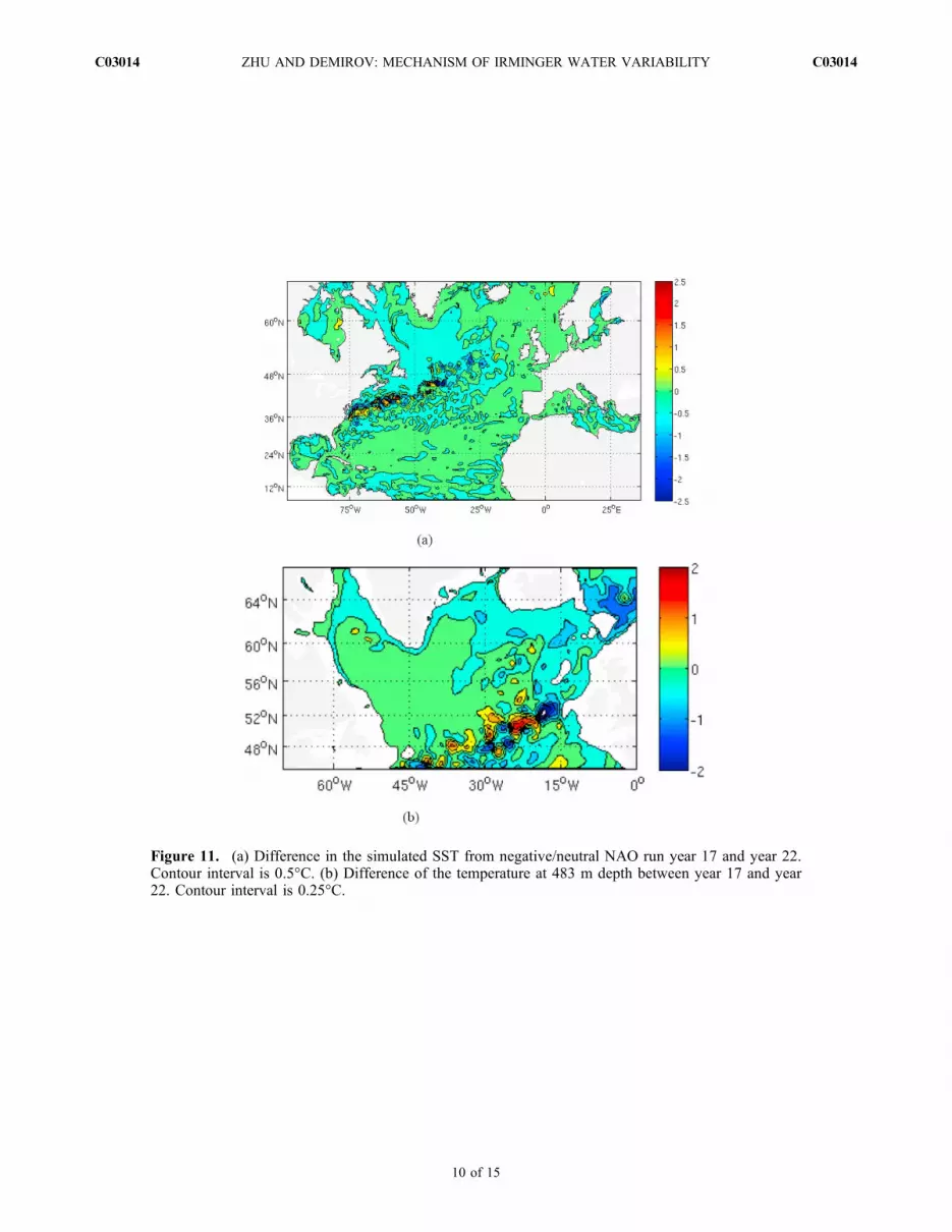
Figure 11. (a) Difference in the simulated SST from negative/neutral NAO run year 17 and year 22.Contour interval is 0.5°C. (b) Difference of the temperature at 483 m depth between year 17 and year22. Contour interval is 0.25°C.


10 of 15

Figure 12. (a) The barotropic stream function averaged over 1958–2005. Contour interval is 5 Sv.(b) The SPGI (blue curve), the first PC of altimetric velocity from Häkkinen and Rhines [2004] (blackcurve), and improved estimation of the first PC of altimetric velocity from Häkkinen et al. [2008] (redcurve). (c) The difference between barotropic stream function fields averaged over 1982–2005 and 1958–1981.


11 of 15

Figure 13. The annual mean temperature along a section of 65°N off the west Greenland coast from1990 to 2005. Contour interval is 0.5°C.


12 of 15

Figure 14. Difference in the simulated SST averaged over 1995–2003 and SST averaged over 1985–1994. Contour interval is 0.2°C.


13 of 15

NAO is in a negative phase. One physical reason for theasymmetric SPG response to decadal variability of theNAO‐like forcing is the difference of mean volume trans-port in the SPG under positive and negative NAO (seeFigure 3c). The mean transport (Figure 3) and the volumeand temperature of IW (Figure 5) in the SPG are higher thannormal in the NAO+ experiment. The relatively warm andsalty subsurface IW in the SPG in the NAO+ experimentintensify the cross‐surface temperature gradients andstrengthens the surface buoyancy fluxes during the coldwinters. Hence, the observed [see Yashayaev, 2007] andsimulated in our model experiments deep convection in theLabrador Sea is most intense in the early 1990s when the

anomalous cold winters occurred during a period of highNAO index (Figure 15a). At the same time in some years inthe second half of period II the NAO index was close toneutral. The transport of IW into the Labrador Sea duringthese earned relatively weak vertical convection contributeto the warming of intermediate layers of the SPG and theweakening of the SPGI. Therefore, during period II,between the cold years with high NAO and relatively warmyears with neutral NAO, the stronger than normal meantransport in the SPG under positive NAO‐like surfaceforcing intensifies the amplitude of decadal variations aswell as covariance between the IWT and intensity of SPGcirculation (Figure 15a).

Figure 15. (a) The SPGI (blue solid curve), the surface temperature averaged over AREA1 (red dottedcurve), and the subsurface temperature off the west Greenland coast (red dashed curve, defined as thetemperature at 483 m averaged 56°W onshore along i65°N). (b) The North Atlantic Oscillation index(data from J. W. Hurrell, available at http://www.cgd.ucar.edu/cas/jhurrell/indices.html).


14 of 15

[27] Acknowledgments. This work was funded by the CanadianFoundation for Climate and Atmospheric Science through projects GOAPPand GR‐631. The discussions with Igor Yashayaev and Amy Bower con-tributed to an improved understanding of the variability in the LabradorSea. We wish to thank Sirpa Häkkinen for providing us with altimeter dataabout the Labrador Sea. The helpful comments of Sarah Lundrigan, JoeWroblewski, and two anonymous reviewers are gratefully acknowledged.

ReferencesBöning, C. W., M. Scheinert, J. Dengg, A. Biastoch, and A. Funk (2006),Decadal variability of subpolar gyre transport and its reverberation in theNorth Atlantic overturning, Geophys. Res. Lett., 33, L21S01, doi:10.1029/2006GL026906.

Brauch, J. P., and R. Gerdes (2005), Response of the northern North Atlanticand Arctic oceans to a sudden change of the North Atlantic Oscillation,J. Geophys. Res., 110, C11018, doi:10.1029/2004JC002436.

Carton, J. A., B. S. Giese, and S. A. Grodsky (2005), Sea level rise and thewarming of the oceans in the Simple OceanDataAssimilation (SODA) oceanreanalysis, J. Geophys. Res., 110, C09006, doi:10.1029/2004JC002817.

Curry, R. G., and M. S. McCartney (2001), Ocean gyre circulation changesassociated with the North Atlantic Oscillation, J. Phys. Oceanogr., 31,3374–3400.

Dengler, M., J. Fischer, F. A. Schott, and R. Zantopp (2006), Deep Labra-dor Current and its variability in 1996–2005, Geophys. Res. Lett., 33,L21S06, doi:10.1029/2006GL026702.

Dickson, R. R., J. Lazier, J. Meincke, P. Rhines, and J. Swift (1996), Long‐term‐coordinated chages in the convective activity of the North Atlantic,Prog. Oceanogr., 38, 241–295.

Eden, C., and J. Willebrand (2001), Mechanism of interannual to decadalvariability of the North Atlantic Circulation, J. Clim., 14, 2266–2280.

Fichefet, T., and M. A. Morales Maqueda (1997), Sensitivity of a global seaice model to the treatment of ice thermodynamics and dynamics, J. Geo-phys. Res., 102, 12,609–12,646.

Greatbatch, R. (2000), The North Atlantic Oscillation, Stochastic Environ.Res. Risk Assess., 14(4), 213–242.

Greatbatch, R. J., A. F. Fanning, A. D. Goulding, and S. Levitus (1991),A diagnosis of interpentadal circulation changes in the North Atlantic,J. Geophys. Res., 96, 22,009–22,023.

Häkkinen, S., and P. B. Rhines (2004), Decline of the North Atlantic sub-polar circulation in the 1990s, Science, 304, 555–559.

Häkkinen, S., H. Hátún, and P. B. Rhines (2008), Satellite evidenceof change in the Northern Gyre, in The Subarctic Seas as a Source of

Arctic Change, edited by R. R. Dickson, J. Meincke, and P. B. Rhines,pp. 551–568, Springer, New York.

Hátún, H., A. B. Sandø, H. Drange, B. Hansen, and H. Valdimarsson(2005), Influence of the Atlantic subpolar gyre on the thermohaline cir-culation, Science, 309, 1841–1844.

Holland, D. M., R. H. Thomas, B. deYoung, B. Lyberth, and M. Ribergaard(2008), Acceleration of Jakobshavn Isbrae triggered by warm subsurfaceIrminger waters, Nat. Geosci., 1, 659–664.

Hurrell, J. W. (1995), Decadal trends in the North Atlantic Oscillation:Regional temperature and precipitation, Science, 269, 676–679.

Kalnay, E., et al. (1996), The NCEP/NCAR 40‐year reanalysis project, Bul.Am. Meteorol. Soc., 77, 437–472.

Lohmann, K., H. Drange, and M. Bentsen (2009), Response of the NorthAtlantic subpolar gyre to persistent North Atlantic oscillation like forc-ing, Clim. Dyn., 32, 273–285.

Madec, G. (2008), NEMO reference manual, ocean dynamics component:NEMO‐OPA. Preliminary version, Note Pole de Modelisation 27, Inst.Pierre‐Simon Laplace, Paris.

Marsh, R., S. A. Josey, B. A. de Cuevas, L. J. Redbourn, and G. D. Quartly(2008), Mechanisms for recent warming of the North Atlantic: Insightsgained with an eddy‐permitting model, J. Geophys. Res., 113, C04031,doi:10.1029/2007JC004096.

Mellor, G. L., C. R. Mechoso, and E. Keto (1982), A diagnostic model of thegeneral circulation of the Atlantic Ocean, Deep Sea Res., 29, 1171–1192.

Myers, P. G., N. Kulan, and M. H. Ribergaard (2007), Irminger Water var-iability in the West Greenland Current, Geophys. Res. Lett., 34, L17601,doi:10.1029/2007GL030419.

Pickart, R. S., D. J. Torres, and R. A. Clarke (2002), Hydrography of theLabrador Sea during active convection, J. Phys. Oceanogr., 32, 428–457.

Thompson, K. R., D. G. Wright, Y. Lu, and E. Demirov (2006), A simplemethod for reducing seasonal bias and drift in eddy resolving ocean mod-els, Ocean Modell., 14, 122–138.

Visbeck, M., E. Chassignet, R. Curry, T. Delworth, B. Dickson, andG. Krahmann (2003), The ocean’s response to North Atlantic Oscillationvariability, in The North Atlantic Oscillation: Climatic Significance andEnvironmental Impact,Geophys.Monogr. Ser., vol. 134, edited by J.Hurrellet al., pp. 113–145, AGU, Washington, D. C.

Yashayaev, I. (2007), Hydrographic changes in the Labrador Sea, 1960–2005, Prog. Oceanogr., 73, 242–276, doi:10.1016/j.pocean.2007.04.015.

E. Demirov and J. Zhu, Department of Physics and Physical Oceanography,Memorial University of Newfoundland, St. John’s, NL A1B 3X7, Canada.([email protected])


15 of 15

Documents

On the mechanism of interannual variability of the Irminger Water in the Labrador Sea