symmetryS S

Article

On the Stability of a Generalized Fréchet Functional Equationwith Respect to Hyperplanes in the Parameter Space

Janusz Brzdek 1,† , Zbigniew Lesniak 2,*,† and Renata Malejki 2,†

�����������������

Citation: Brzdek, J.; Lesniak, Z.;

Malejki, R. On the Stability of a

Generalized Fréchet Functional

Equation with Respect to

Hyperplanes in the Parameter Space.

Symmetry 2021, 13, 384. https://

doi.org/10.3390/sym13030384

Academic Editor: Sun Young Cho

Received: 8 February 2021

Accepted: 24 February 2021

Published: 27 February 2021

Publisher’s Note: MDPI stays neutral

with regard to jurisdictional claims in

published maps and institutional affil-

iations.

Copyright: © 2021 by the authors.

Licensee MDPI, Basel, Switzerland.

This article is an open access article

distributed under the terms and

conditions of the Creative Commons

Attribution (CC BY) license (https://

creativecommons.org/licenses/by/

4.0/).

1 Faculty of Applied Mathematics, AGH University of Science and Technology, Mickiewicza 30,30-059 Kraków, Poland; brzdek@agh.edu.pl

2 Department of Mathematics, Pedagogical University, Podchorazych 2, 30-084 Kraków, Poland;renata.malejki1@student.up.krakow.pl

* Correspondence: zbigniew.lesniak@up.krakow.pl† These authors contributed equally to this work.

Abstract: We study the Ulam-type stability of a generalization of the Fréchet functional equation.Our aim is to present a method that gives an estimate of the difference between approximate andexact solutions of this equation. The obtained estimate depends on the values of the coefficients ofthe equation and the form of the control function. In the proofs of the main results, we use a fixedpoint theorem to get an exact solution of the equation close to a given approximate solution.

Keywords: stability; inner product space; fixed point theorem; Fréchet equation

1. Introduction

In this paper, we study the functional equation:

A1F(x + y + z) + A2F(x) + A3F(y) + A4F(z) = A5F(x + y) + A6F(x + z) + A7F(y + z), (1)

where A1, . . . , A7 ∈ K are constants and K denotes the fields of real or complex numbers,in the class of functions F : X → Y from a commutative group X into a Banach space Yover the field K. This equation is a generalization of the following equation:

F(x + y + z) + F(x) + F(y) + F(z) = F(x + y) + F(x + z) + F(y + z). (2)

Equation (2) was used by Fréchet [1] to obtain a characterization the inner productspaces among normed linear spaces, and it is called the Fréchet functional equation.For more results concerning the relationship of Equation (2) with inner product spaces,we refer to [2–8]. Equation (1) is a linear generalization of Equation (2). A nonlineargeneralization of the Fréchet functional Equation (2) was considered in [9].

The set of solutions of Equation (1) was studied in [10]. The main result of that papersays that if Ai 6= Aj for some i, j ∈ {1, ..., 7}, then each solution of Equation (1) such thatF(0) = 0 is an additive function. In fact, under the assumption that Ai 6= Aj for somei, j ∈ {1, ..., 7}, every solution F of Equation (1) is of the form F = a + c, where a is anadditive function and c is a constant.

In this paper, we investigate the problem of the stability of Equation (1) consideringpossible values of coefficients Ai for i ∈ {1, ..., 7}. Roughly speaking, for an approximatesolution of Equation (1), we are looking for an exact solution of this equation that is close tothe given approximate solution. Some results in this direction obtained under assumptionson some coefficients Ai can be found in [10,11]. The Ulam-type stability problem forfunctional, difference, differential, and integral equations was described in more detail inthe monographs [12–14] and survey papers [15,16]. For a comparison of the stability resultsfor functional equations related to the functional equation considered here, the reader isalso referred to [17–28].

Symmetry 2021, 13, 384. https://doi.org/10.3390/sym13030384 https://www.mdpi.com/journal/symmetry

Symmetry 2021, 13, 384 2 of 21

Equation (1) can be treated as a special case of the general linear equation. The stabilityproblem of the general linear equation was studied in [29–32]. In this article, we want tolook at Equation (1) in order to get estimates of the difference between approximate andexact solutions more closely connected to the values of the coefficients of the equation andthe form of the control function.

Let us consider the following system of linear equations:

A2 + A3 + A4 = 0A1 + A2 + A3 = 0A1 + A2 + A4 = 0A1 + A3 + A4 = 0−A2 − A3 + A6 + A7 = 0−A2 − A4 + A5 + A7 = 0−A3 − A4 + A5 + A6 = 0.

(3)

Its matrix is the form:

0 1 1 1 0 0 01 1 1 0 0 0 01 1 0 1 0 0 01 0 1 1 0 0 00 −1 −1 0 0 1 10 −1 0 −1 1 0 10 0 −1 −1 1 1 0

.

The determinant of this matrix is equal to six. Therefore, in the case where not all parametersA1, . . . , A7 are equal to zero, at least one of the equations of System (3) is not satisfied.

In [10], the stability of Equation (1) was proven under the assumption that A2 + A3 +A4 6= 0. In this paper, we consider the remaining six cases corresponding to the equations ofSystem (3). They can be grouped into two classes so that each would contain similar cases.The division into classes is made due to the symmetry of substitutions for the variablesoccurring in Equation (1). We formulate stability results for one case from each class.

Now, we list the appropriate substitutions, the equations obtained from Equation (1)by using these substitutions, and the form of an operator that can be used in a proof of thestability result corresponding to consecutive cases:

(I) x = t, y = t, z = t

A1F(3t) + (A2 + A3 + A4)F(t) = (A5 + A6 + A7)F(2t), (4)

F(t) =A5 + A6 + A7

A2 + A3 + A4F(2t)− A1

A2 + A3 + A4F(3t)

(II) x = t, y = t, z = −t

(A1 + A2 + A3)F(t) + A4F(−t) = A5F(2t) + (A6 + A7)F(0), (5)

F(t) =A5

A1 + A2 + A3F(2t) +

A6 + A7

A1 + A2 + A3F(0)− A4

A1 + A2 + A3F(−t),

(III) x = t, y = −t, z = t

(A1 + A2 + A4)F(t) + A3F(−t) = (A5 + A7)F(0) + A6F(2t), (6)

F(t) =A5 + A7

A1 + A2 + A4F(0) +

A6

A1 + A2 + A4F(2t)− A3

A1 + A2 + A4F(−t),

(IV) x = −t, y = t, z = t

(A1 + A3 + A4)F(t) + A2F(−t) = (A5 + A6)F(0) + A7F(2t), (7)

Symmetry 2021, 13, 384 3 of 21

F(t) =A5 + A6

A1 + A3 + A4F(0) +

A7

A1 + A3 + A4F(2t)− A2

A1 + A3 + A4F(−t),

(V) x = t, y = t, z = 0

(A6 + A7 − A2 − A3)F(t) = (A1 − A5)F(2t) + A4F(0), (8)

F(t) =A1 − A5

A6 + A7 − A2 − A3F(2t) +

A4

A6 + A7 − A2 − A3F(0),

(VI) x = t, y = 0, z = t

(A5 + A7 − A2 − A4)F(t) = (A1 − A6)F(2t) + A3F(0), (9)

F(t) =A1 − A6

A5 + A7 − A2 − A4F(2t) +

A3

A5 + A7 − A2 − A4F(0),

(VII) x = 0, y = t, z = t

(A5 + A6 − A3 − A4)F(t) = (A1 − A7)F(2t) + A2F(0), (10)

F(t) =A1 − A7

A5 + A6 − A3 − A4F(2t) +

A2

A5 + A6 − A3 − A4F(0).

As mentioned above, Case (I) was considered in [10]. In this paper, we deal with Cases(II) and (V) chosen from classes consisting of Cases (II)–(IV) and (V)–(VII), respectively.The remaining cases in each class are analogous to those selected.

The proofs of our results are based on the fixed point theorem quoted below. The fixedpoint approach to the Ulam-type stability problem can also be found in, e.g., [33–36].

Theorem 1 ([37]). Let the following three hypotheses be valid.

(H1) S is a nonempty set; E is a Banach space; and functions f1, ..., fk : S→ S and l1, . . . , lk : S→R+ are given, where R+ denotes the set of nonnegative reals.

(H2) T : ES → ES is an operator satisfying the inequality:

∥∥T ξ(x)− T µ(x)∥∥ ≤ k

∑i=1

li(x)∥∥ξ( fi(x))− µ( fi(x))

∥∥, ξ, µ ∈ ES, x ∈ S. (11)

(H3) Λ : R+S → R+

S is defined by:

Λδ(x) :=k

∑i=1

li(x)δ( fi(x)), δ ∈ R+S, x ∈ S.

Assume that functions ε : S→ R+ and ϕ : S→ E fulfil the following two conditions:∥∥T ϕ(x)− ϕ(x)∥∥ ≤ ε(x), x ∈ S, (12)

ε∗(x) :=∞

∑n=0

Λnε(x) < ∞, x ∈ S. (13)

Then, there exists a unique fixed point ψ of T with:

‖ϕ(x)− ψ(x)‖ ≤ ε∗(x), x ∈ S. (14)

Moreover,ψ(x) := lim

n→∞T n ϕ(x), x ∈ S. (15)

Symmetry 2021, 13, 384 4 of 21

2. The Main Results

In this section, we prove the stability results for two chosen cases from the above list.In Case (II), we assume that X is a commutative group. However, in Case (V), we can workunder the more general assumption. Namely, similar to Case (I) considered in [10], weassume that X is a commutative monoid.

We start with Case (II), which corresponds to the second equation of System (3).

Theorem 2. Let (X,+) be an abelian group, Y be a Banach space, and A1, . . . , A7 ∈ K ∈ {R,C}.Assume that A1 + A2 + A3 6= 0. Let a function L : X3 → [0, ∞) satisfy the condition:

L(kx, ky, kz) ≤ c(k)L(x, y, z), (x, y, z) ∈ X3, k ∈ {2, 0,−1}, (16)

with c(2), c(0), c(−1) ∈ [0, ∞) such that b := c(2)d(2) + c(0)d(0) + c(−1)d(−1) < 1, where:

d(2) :=∣∣∣∣ A5

A1 + A2 + A3

∣∣∣∣, d(0) :=∣∣∣∣ A6 + A7

A1 + A2 + A3

∣∣∣∣, d(−1) :=∣∣∣∣ A4

A1 + A2 + A3

∣∣∣∣. (17)

Assume that f : X → Y is a function such that:

‖A1 f (x + y + z) + A2 f (x) + A3 f (y) + A4 f (z)− A5 f (x + y)− A6 f (x + z) (18)

− A7 f (y + z)‖ ≤ L(x, y, z), (x, y, z) ∈ X3.

Then, there exists a unique function F : X → Y satisfying (1) such that:

‖ f (x)− F(x)‖ ≤ ρL(x), x ∈ X, (19)

where:

ρL(x) :=L(x, x,−x)

|A1 + A2 + A3|(1− b), x ∈ X. (20)

Proof. Taking x = y = t, z = −t in (18), we obtain:

‖(A1 + A2 + A3) f (t) + A4 f (−t)− A5 f (2t)− (A6 + A7) f (0)‖ ≤ L(t, t,−t), t ∈ X.

Hence, for each x ∈ X:∥∥∥∥ f (t) +A4

A1 + A2 + A3f (−t)− A5

A1 + A2 + A3f (2t)− A6 + A7

A1 + A2 + A3f (0)

∥∥∥∥ ≤ ε(t), (21)

where ε(t) := L(t,t,−t)|A1+A2+A3|

. Put:

T ξ(t) :=A5

A1 + A2 + A3ξ(2t) +

A6 + A7

A1 + A2 + A3ξ(0)− A4

A1 + A2 + A3ξ(−t), ξ ∈ YX , t ∈ X. (22)

Let us note that the operator T is linear. From (21), we get that:

‖ f (t)− T f (t)‖ ≤ ε(t), t ∈ X.

Symmetry 2021, 13, 384 5 of 21

Fix ξ, µ ∈ YX . For every t ∈ X, we have:

‖T ξ(t)− T µ(t)‖ =∥∥∥∥ A5

A1 + A2 + A3(ξ(2t)− µ(2t)) +

A6 + A7

A1 + A2 + A3(ξ(0)− µ(0))

− A4

A1 + A2 + A3(ξ(−t)− µ(−t))

∥∥∥∥≤∣∣∣∣ A5

A1 + A2 + A3

∣∣∣∣‖ξ(−2t)− µ(−2t)‖+∣∣∣∣ A6 + A7

A1 + A2 + A3

∣∣∣∣‖ξ(0)− µ(0)‖

+

∣∣∣∣ A4

A1 + A2 + A3

∣∣∣∣‖ξ(−t)− µ(−t)‖.

Thus:

‖T ξ(t) − T µ(t)‖ ≤ d(2)‖ξ(2t)− µ(2t)‖+ d(0)‖ξ(0)− µ(0)‖+ d(−1)‖ξ(−t)− µ(−t)‖, t ∈ X. (23)

We showed that Condition (H2) is satisfied with k = 3, S = X, E = Y,

f1(t) = 2t, f2(t) = 0, f3(t) = −t,

l1(t) = d(2), l2(t) = d(0), l3(t) = d(−1),

i.e.,:

‖T ξ(t) − T µ(t)‖ ≤3

∑i=1

li(t)‖ξ( fi(t))− µ( fi(t))‖, ξ, η ∈ YX , t ∈ X.

Define an operator Λ : R+X → R+

X by:

Λη(t) :=3

∑i=1

li(t)η( fi(t)), t ∈ X

for every η ∈ R+X . Then, for each η ∈ R+

X , we have:

Λη(t) = d(2)η(2t) + d(0)η(0) + d(−1)η(−t), t ∈ X.

Let us note that the operator Λ is monotone, i.e.,: for all η, ζ ∈ R+X , if η ≤ ζ, then Λη ≤ Λζ.

Moreover, by (23):

‖T ξ(t)− T µ(t)‖ ≤ Λ(‖ξ − µ‖)(t), ξ, µ ∈ YX , t ∈ X. (24)

Symmetry 2021, 13, 384 6 of 21

Now, we show that ε∗(t) := ∑∞n=0 Λnε(t) < ∞ for each t ∈ X, i.e., the function series

∑∞n=0 Λnε(t) is convergent for each t ∈ X. Fix a t ∈ X. In view of (16), we have:

Λε(t) = d(2)ε(2t) + d(0)ε(0) + d(−1)ε(−t)

= d(2)L(2t, 2t,−2t))|A1 + A2 + A3|

+ d(0)L(0, 0, 0)

|A1 + A2 + A3|

+ d(−1)L(−(t, t,−t))|A1 + A2 + A3|

≤ d(2)c(2)L(t, t,−t)

|A1 + A2 + A3|+ d(0)c(0)

L(t, t,−t)|A1 + A2 + A3|

+ d(−1)c(−1)L(t, t,−t)

|A1 + A2 + A3|

= (d(2)c(2) + d(0)c(0) + d(−1)c(−1))L(t, t,−t)

|A1 + A2 + A3|.

Thus:

Λε(t) ≤ bε(t), t ∈ X. (25)

By induction, we show that:

Λnε(t) ≤ bnε(t), t ∈ X, n ∈ N. (26)

For n = 1, Condition (26) coincides with Condition (25). For n = 2, by the monotonicityand linearity of Λ, we get from (25):

Λ2ε(t) = Λ(Λε)(t) ≤ Λ(bε)(t) = bΛε(t) ≤ b2ε(t)

for all t ∈ X. Now, suppose that (26) holds for some n ∈ N. Then, for every t ∈ X, we have:

Λn+1ε(t) = Λ(Λnε)(t) ≤ Λ(bnε)(t) = bnΛε(t) ≤ bn+1ε(t).

From (26), we receive the following estimate for each t ∈ X:

ε∗(t) =∞

∑n=0

Λnε(t) ≤∞

∑n=0

bnε(t) =ε(t)

1− b=

L(t, t,−t)|A1 + A2 + A3|(1− b)

.

By Theorem 1 (with S = X and E = Y), there exists a function F : X → Y such that:

F(t) =A5

A1 + A2 + A3F(2t) +

A6 + A7

A1 + A2 + A3F(0)− A4

A1 + A2 + A3F(−t), t ∈ X, (27)

and:

‖ f (t)− F(t)‖ ≤ ε∗(t) ≤ L(t, t,−t)|A1 + A2 + A3|(1− b)

, t ∈ X. (28)

Moreover,

F(t) = limn→∞

T n f (t), t ∈ X.

Next, by induction, we show that for every (x, y, z) ∈ X3, n ∈ N0 := N∪ {0}:

‖A1T n f (x + y + z) + A2T n f (x) + A3T n f (y) + A4T n f (z) (29)

− A5T n f (x + y)− A6T n f (x + z)− A7T n f (y + z)‖≤ bn L(x, y, z), (x, y, z) ∈ X3.

Symmetry 2021, 13, 384 7 of 21

For n = 0, Condition (29) is simply (18). For n = 1 using (22), we have:∥∥A1T f (x + y + z) + A2T f (x) + A3T f (y) + A4T f (z)

A5T f (x + y)− A6T f (x + z)− A7T f (y + z)∥∥

=∥∥ A5

A1 + A2 + A3A1 f (2(x + y + z)) +

A6 + A7

A1 + A2 + A3A1 f (0))

− A4

A1 + A2 + A3A1 f (−(x + y + z))

+A5

A1 + A2 + A3A2 f (2x) +

A6 + A7

A1 + A2 + A3A2 f (0)

− A3

A1 + A2 + A3A2 f (−x)

+A5

A1 + A2 + A3A3 f (2y) +

A6 + A7

A1 + A2 + A3A3 f (0)

− A4

A1 + A2 + A3A3 f (−y)

+A5

A1 + A2 + A3A4 f (2z) +

A6 + A7

A1 + A2 + A3A4 f (0)

− A4

A1 + A2 + A3A4 f (−z)

− A5

A1 + A2 + A3A5 f (2(x + y))− A6 + A7

A1 + A2 + A3A5 f (0)

+A4

A1 + A2 + A3A5 f (−1(x + y))

− A5

A1 + A2 + A3A6 f (2(x + z))− A6 + A7

A1 + A2 + A3A6 f (0)

+A4

A1 + A2 + A3A5 f (−1(x + z))

− A5

A1 + A2 + A3A7 f (2(y + z))− A6 + A7

A1 + A2 + A3A7 f (0)

+A4

A1 + A2 + A3A7 f (−1(y + z))

∥∥≤

∣∣∣∣ A5

A1 + A2 + A3

∣∣∣∣L(2x, 2y, 2z) +∣∣∣∣ A6 + A7

A1 + A2 + A3

∣∣∣∣L(0, 0, 0)

+

∣∣∣∣ A4

A1 + A2 + A3

∣∣∣∣L(−x,−y,−z)

≤ (d(2)c(2) + d(0)c(0) + d(−1)c(−1))L(x, y, z)

= bL(x, y, z).

Now, suppose that (29) holds for some n ∈ N0. Then, for every (x, y, z) ∈ X3, we have:

Symmetry 2021, 13, 384 8 of 21

∥∥A1T n+1 f (x + y + z) + A2T n+1 f (x) + A3T n+1 f (y) + A4T n+1 f (z)

A5T n+1 f (x + y)− A6T n+1 f (x + z)− A7T n+1 f (y + z)∥∥

=∥∥ A5

A1 + A2 + A3A1T n f (2(x + y + z)) +

A6 + A7

A1 + A2 + A3A1T n f (0))

− A4

A1 + A2 + A3A1T n f (−(x + y + z))

+A5

A1 + A2 + A3A2T n f (2x) +

A6 + A7

A1 + A2 + A3A2T n f (0)

− A3

A1 + A2 + A3A2T n f (−x)

+A5

A1 + A2 + A3A3T n f (2y) +

A6 + A7

A1 + A2 + A3A3T n f (0)

− A4

A1 + A2 + A3A3T n f (−y)

+A5

A1 + A2 + A3A4T n f (2z) +

A6 + A7

A1 + A2 + A3A4T n f (0)

− A4

A1 + A2 + A3A4T n f (−z)

− A5

A1 + A2 + A3A5T n f (2(x + y))− A6 + A7

A1 + A2 + A3A5T n f (0)

+A4

A1 + A2 + A3A5T n f (−1(x + y))

− A5

A1 + A2 + A3A6T n f (2(x + z))− A6 + A7

A1 + A2 + A3A6T n f (0)

+A4

A1 + A2 + A3A5T n f (−1(x + z))

− A5

A1 + A2 + A3A7T n f (2(y + z))− A6 + A7

A1 + A2 + A3A7T n f (0)

+A4

A1 + A2 + A3A7T n f (−1(y + z))

∥∥≤

(∣∣∣∣ A5

A1 + A2 + A3

∣∣∣∣bnL(2x, 2y, 2z) +∣∣∣∣ A6 + A7

A1 + A2 + A3

∣∣∣∣bnL(0, 0, 0)

+

∣∣∣∣ A4

A1 + A2 + A3

∣∣∣∣bnL(−x,−y,−z))

≤ bn(d(2)c(2) + d(0)c(0) + d(−1)c(−1))L(x, y, z)

= bn+1L(x, y, z).

Thus, by induction, we obtain Condition (29). Letting n→ ∞ in (29), we get:

A1F (x + y + z) + A2F(x) + A3F(y) + A4F(z) (30)

= A5F(x + y) + A6F(x + z) + A7F(y + z), (x, y, z) ∈ X3.

Thus, we proved that there exists a function F : X → Y satisfying Equation (1) for allx, y, z ∈ X and such that:

‖ f (x)− F(x)‖ ≤ ε∗(x) ≤ ρL(x), x ∈ X. (31)

Finally, we prove the uniqueness of the exact solution F satisfying (19). To this end,we show by induction that for every n ∈ N:

‖T nξ(x)− T nµ(x)‖ ≤ Λn(‖ξ − µ‖)(x), ξ, µ ∈ YX , x ∈ X. (32)

Symmetry 2021, 13, 384 9 of 21

For n = 1, Condition (32) is simply (24). For n = 2 using (24) and the monotonicity of Λ,we have:

‖T 2ξ(x)− T 2µ(x)‖ = ‖T (T ξ)(x)− T (T µ)(x)‖ ≤ Λ(‖T ξ − T µ‖)(x)

≤ Λ(Λ(‖ξ − µ‖))(x) = Λ2(‖ξ − µ‖)(x), x ∈ X

for ξ, µ ∈ YX. Fix ξ, µ ∈ YX, and assume that for an n ∈ N, Relation (32) holds. Then,by (24):

‖T n+1ξ(x)− T n+1µ(x)‖ = ‖T (T nξ)(x)− T (T nµ)(x)‖≤ Λ(‖T nξ − T nµ‖)(x), x ∈ X.

Hence, by the inductive hypothesis and the monotonicity of Λ, we obtain:

‖T n+1ξ(x)− T n+1µ(x)‖ ≤ Λ(Λn(‖ξ − µ‖))(x) = Λn+1(‖ξ − µ‖)(x), x ∈ X.

Let G : X → Y be also a solution of (1) such that ‖ f (x)− G(x)‖ ≤ ρL(x) for x ∈ X.Then:

‖G(x)− F(x)‖ ≤ 2ρL(x), x ∈ X. (33)

Hence, by (32), we obtain:

‖T nG(x)− T nF(x)‖ ≤ 2ΛnρL(x) ≤ 2Λnε(x)1− γ(x)

, x ∈ X,

since Λ is linear and monotone. Letting n → ∞, by the convergence of the series∑∞

n=0 Λnε(x), we get:

limn→∞

‖T nG(x)− T nF(x)‖ = 0, x ∈ X.

Hence, ‖G(x)− F(x)‖ = 0 for x ∈ X, since G and F are fixed points of T . Consequently,G(x) = F(x) for every x ∈ X.

Let us point out that the numerator |A6 + A7| of the constant d(0) can be muchsmaller than the sum |A6| + |A7| in the case where the numbers A6, A7 have oppositesigns. Therefore, for some values of coefficients Ai, the above theorem can give the betterapproximation of the exact solution of Equation (1) than the known results. Moreover,replacing |A6|+ |A7| with |A6 + A7| causes a larger set of coefficients to be covered by thestability results, since the above theorem contains the assumption b < 1, and analogousassumptions occur in the known results concerning the stability of more general equations.

Let us note that if L(0, 0, 0) 6= 0, then by (16), we get that c(0) ≥ 1. However, in thecase where L(0, 0, 0) = 0, without loss of generality, we can put c(0) = 0. Then, the constantb occurring in (20) is of the form:

b = c(2)d(2) + c(−1)d(−1), (34)

where d(2) and d(−1) are given by (17). Hence, if A4 = A5 = 0, then d(2) = d(−1) = 0.Thus, b = 0, and consequently, ε∗(x) = ε(x). In this case, we can easily determine the exactsolution of the considered functional equation.

Corollary 1. Let (X,+) be an abelian group, Y be a Banach space, and A1, . . . , A7 ∈ K ∈ {R,C}.Assume that A1 + A2 + A3 6= 0 and A4 = A5 = 0. Let a function L : X3 → [0, ∞) satisfy theconditions L(0, 0, 0) = 0 and:

Symmetry 2021, 13, 384 10 of 21

L(kx, ky, kz) ≤ c(k)L(x, y, z), (x, y, z) ∈ X3, k ∈ {2,−1},

with some c(2), c(−1) ∈ [0, ∞). Assume that f : X → Y is a function such that Condition (18) isfulfilled. Then, there exists a unique function F : X → Y satisfying (1) such that:

‖ f (x)− F(x)‖ ≤ ρL(x), x ∈ X,

where:

ρL(x) :=L(x, x,−x)|A1 + A2 + A3|

, x ∈ X.

Moreover, F is a constant function given by the formula:

F(x) =A6 + A7

A1 + A2 + A3f (0), x ∈ X. (35)

Proof. From (22), under our assumption on coefficients Ai, we get that:

T ξ(t) =A6 + A7

A1 + A2 + A3ξ(0), ξ ∈ YX , t ∈ X.

Moreover, by (27), we have:

F(t) =A6 + A7

A1 + A2 + A3F(0), t ∈ X. (36)

By (17) and (34), we obtain that b = 0. Hence, by (26):

Λnε(t) = 0, t ∈ X, n ∈ N,

where:

ε(t) =L(t, t,−t)

|A1 + A2 + A3|, t ∈ X.

From (28), we obtain that F(0) = f (0), since L(0, 0, 0) = 0. Hence, by (36), we getFormula (35).

Now, we proceed to Case (V).

Theorem 3. Let (X,+) be a commutative monoid, Y be a Banach space, and A1, . . . , A7 ∈ K ∈{R,C}. Assume that −A2 − A3 + A6 + A7 6= 0. Let a function L : X3 → [0, ∞) satisfythe condition:

L(kx, ky, kz) ≤ c(k)L(x, y, z), (x, y, z) ∈ X3, k ∈ {0, 2}, (37)

with c(2), c(0) ∈ [0, ∞) such that b := c(2)d(2) + c(0)d(0) < 1, where:

d(2) :=∣∣∣∣ A1 − A5

A6 + A7 − A2 − A3

∣∣∣∣, d(0) :=∣∣∣∣ A4

A6 + A7 − A2 − A3

∣∣∣∣. (38)

Assume that f : X → Y is a function such that Condition (18) is fulfilled. Then, there exists aunique function F : X → Y satisfying (1) such that Condition (19) holds, where:

ρL(x) :=L(x, x, 0)

|A6 + A7 − A2 − A3|(1− b), x ∈ X. (39)

Symmetry 2021, 13, 384 11 of 21

Proof. Taking x = t, y = t, z = 0 in (18), we obtain:

‖(A6 + A7 − A2 − A3) f (t)− (A1 − A5) f (2t) + A4 f (0)‖ ≤ L(t, t, 0), t ∈ X.

Hence, for each x ∈ X:∥∥∥∥ f (t)− A1 − A5

A6 + A7 − A2 − A3f (2t)− A4

A6 + A7 − A2 − A3f (0)

∥∥∥∥ ≤ ε(t), (40)

where ε(t) := L(t,t,0)|A6+A7−A2−A3|

. Put:

T ξ(t) :=A1 − A5

A6 + A7 − A2 − A3ξ(2t) +

A4

A6 + A7 − A2 − A3ξ(0), ξ ∈ YX , t ∈ X. (41)

Let us note that the operator T is linear. From (40), we get that:

‖ f (t)− T f (t)‖ ≤ ε(t), t ∈ X.

Fix ξ, µ ∈ YX . For every t ∈ X, we have:

‖T ξ(t)− T µ(t)‖ =∥∥∥∥ A1 − A5

A6 + A7 − A2 − A3(ξ(2t)− µ(2t)) +

A4

A6 + A7 − A2 − A3(ξ(0)− µ(0))

∥∥∥∥≤∣∣∣∣ A1 − A5

A6 + A7 − A2 − A3

∣∣∣∣‖ξ(2t)− µ(2t)‖

+

∣∣∣∣ A4

A6 + A7 − A2 − A3

∣∣∣∣‖ξ(0)− µ(0)‖.

Thus:

‖T ξ(t) − T µ(t)‖ ≤ d(2)‖ξ(2t)− µ(2t)‖+ d(0)‖ξ(0)− µ(0)‖, t ∈ X. (42)

We have shown that Condition (H2) is satisfied with k = 2, S = X, E = Y,

f1(t) = 2t, f2(t) = 0, l1(t) = d(2), l2(t) = d(0),

i.e.,:

‖T ξ(t) − T µ(t)‖ ≤2

∑i=1

li(t)‖ξ( fi(t))− µ( fi(t))‖, ξ, µ ∈ YX , t ∈ X.

Define an operator Λ : R+X → R+

X by:

Λη(t) :=2

∑i=1

li(t)η( fi(t)), t ∈ X

for every η ∈ R+X . Then, for each η ∈ R+

X , we have:

Λη(t) := d(2)η(2t) + d(0)η(0), t ∈ X.

Let us note that the operator Λ is monotone, i.e., for all η, ζ ∈ R+X if η ≤ ζ, then Λη ≤ Λζ.

Moreover, by (42):

‖T ξ(t)− T µ(t)‖ ≤ Λ(‖ξ − µ‖)(t), ξ, µ ∈ YX , t ∈ X. (43)

Symmetry 2021, 13, 384 12 of 21

Now, we show that ε∗(t) := ∑∞n=0 Λnε(t) < ∞ for each t ∈ X, i.e., the function series

∑∞n=0 Λnε(t) is convergent for each t ∈ X. Fix a t ∈ X. In view of (37), we have:

Λε(t) = d(2)ε(2t) + d(0)ε(0)

= d(2)L(2t, 2t, 0)

|A6 + A7 − A2 − A3|+ d(0)

L(0, 0, 0)|A6 + A7 − A2 − A3|

≤ d(2)c(2)L(t, t, 0)

|A6 + A7 − A2 − A3|+ d(0)c(0)

L(t, t, 0)|A6 + A7 − A2 − A3|

= (d(2)c(2) + d(0)c(0))L(t, t, 0)

|A6 + A7 − A2 − A3|.

Thus:

Λε(t) ≤ bε(t), t ∈ X. (44)

By induction, we show that:

Λnε(t) ≤ bnε(t), t ∈ X. (45)

For n = 1, Condition (45) coincides with Condition (44). For n = 2, by the monotonicityand linearity of Λ, we get from (44):

Λ2ε(t) = Λ(Λε)(t) ≤ Λ(bε)(t) = bΛε(t) ≤ b2ε(t)

for all t ∈ X. Now, suppose that (45) holds for some n ∈ N. Then, for every t ∈ X, usingthe inductive hypothesis, we have:

Λn+1ε(t) = Λ(Λnε)(t) ≤ Λ(bnε)(t) = bnΛε(t) ≤ bn+1ε(t).

Using (45), we obtain:

ε∗(t) =∞

∑n=0

Λnε(t) ≤∞

∑n=0

bnε(t) =ε(t)

1− b=

L(t, t, 0)|A6 + A7 − A2 − A3|(1− b)

for each t ∈ X. By Theorem 1 (with S = X and E = Y), there exists a function F : X → Ysuch that:

F(t) =A1 − A5

A6 + A7 − A2 − A3F(2t) +

A4

A6 + A7 − A2 − A3F(0), t ∈ X,

and:

‖ f (t)− F(t)‖ ≤ ε∗(t) ≤ L(t, t, 0)|A6 + A7 − A2 − A3|(1− b)

, t ∈ X.

Moreover,F(t) = lim

n→∞T n f (t), t ∈ X.

Next, by induction, we show that for every (x, y, z) ∈ X3, n ∈ N0 := N∪ {0}:

‖A1T n f (x + y + z) + A2T n f (x) + A3T n f (y) + A4T n f (z) (46)

− A5T n f (x + y)− A6T n f (x + z)− A7T n f (y + z)‖≤ bn L(x, y, z), (x, y, z) ∈ X3.

For n = 0, Condition (46) is simply (18). For n = 1 using (41), we have:

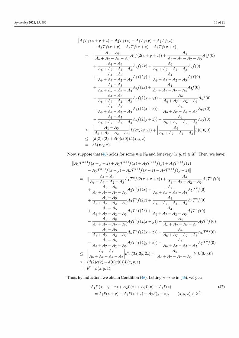
Symmetry 2021, 13, 384 13 of 21

∥∥A1T f (x + y + z) + A2T f (x) + A3T f (y) + A4T f (z)

− A5T f (x + y)− A6T f (x + z)− A7T f (y + z)∥∥

=∥∥ A1 − A5

A6 + A7 − A2 − A3A1 f (2(x + y + z)) +

A4

A6 + A7 − A2 − A3A1 f (0)

+A1 − A5

A6 + A7 − A2 − A3A2 f (2x) +

A4

A6 + A7 − A2 − A3A2 f (0)

+A1 − A5

A6 + A7 − A2 − A3A3 f (2y) +

A4

A6 + A7 − A2 − A3A3 f (0)

+A1 − A5

A6 + A7 − A2 − A3A4 f (2z) +

A4

A6 + A7 − A2 − A3A4 f (0)

− A1 − A5

A6 + A7 − A2 − A3A5 f (2(x + y))− A4

A6 + A7 − A2 − A3A5 f (0)

− A1 − A5

A6 + A7 − A2 − A3A6 f (2(x + z))− A4

A6 + A7 − A2 − A3A6 f (0)

− A1 − A5

A6 + A7 − A2 − A3A7 f (2(y + z))− A4

A6 + A7 − A2 − A3A7 f (0)

≤∣∣∣∣ A1 − A5

A6 + A7 − A2 − A3

∣∣∣∣L(2x, 2y, 2z) +∣∣∣∣ A4

A6 + A7 − A2 − A3

∣∣∣∣L(0, 0, 0)

≤ (d(2)c(2) + d(0)c(0))L(x, y, z)

= bL(x, y, z).

Now, suppose that (46) holds for some n ∈ N0 and for every (x, y, z) ∈ X3. Then, we have:∥∥A1T n+1 f (x + y + z) + A2T n+1 f (x) + A3T n+1 f (y) + A4T n+1 f (z)

− A5T n+1 f (x + y)− A6T n+1 f (x + z)− A7T n+1 f (y + z)∥∥

=∥∥ A1 − A5

A6 + A7 − A2 − A3A1T n f (2(x + y + z)) +

A4

A6 + A7 − A2 − A3A1T n f (0)

+A1 − A5

A6 + A7 − A2 − A3A2T n f (2x) +

A4

A6 + A7 − A2 − A3A2T n f (0)

+A1 − A5

A6 + A7 − A2 − A3A3T n f (2y) +

A4

A6 + A7 − A2 − A3A3T n f (0)

+A1 − A5

A6 + A7 − A2 − A3A4T n f (2z) +

A4

A6 + A7 − A2 − A3A4T n f (0)

− A1 − A5

A6 + A7 − A2 − A3A5T n f (2(x + y))− A4

A6 + A7 − A2 − A3A5T n f (0)

− A1 − A5

A6 + A7 − A2 − A3A6T n f (2(x + z))− A4

A6 + A7 − A2 − A3A6T n f (0)

− A1 − A5

A6 + A7 − A2 − A3A7T n f (2(y + z))− A4

A6 + A7 − A2 − A3A7T n f (0)

≤∣∣∣∣ A1 − A5

A6 + A7 − A2 − A3

∣∣∣∣bnL(2x, 2y, 2z) +∣∣∣∣ A4

A6 + A7 − A2 − A3

∣∣∣∣bnL(0, 0, 0

)≤ (d(2)c(2) + d(0)c(0))L(x, y, z)

= bn+1L(x, y, z).

Thus, by induction, we obtain Condition (46). Letting n→ ∞ in (46), we get:

A1F (x + y + z) + A2F(x) + A3F(y) + A4F(z) (47)

= A5F(x + y) + A6F(x + z) + A7F(y + z), (x, y, z) ∈ X3.

Symmetry 2021, 13, 384 14 of 21

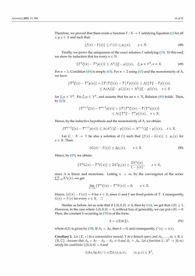
Therefore, we proved that there exists a function F : X → Y satisfying Equation (1) for allx, y, z ∈ X and such that:

‖ f (x)− F(x)‖ ≤ ε∗(x) ≤ ρL(x), x ∈ X. (48)

Finally, we prove the uniqueness of the exact solution F satisfying (19). To this end,we show by induction that for every n ∈ N:

‖T nξ(x)− T nµ(x)‖ ≤ Λn(‖ξ − µ‖)(x), ξ, µ ∈ YX , x ∈ X. (49)

For n = 1, Condition (49) is simply (43). For n = 2 using (43) and the monotonicity of Λ,we have:

‖T 2ξ(x)− T 2µ(x)‖ = ‖T (T ξ)(x)− T (T µ)(x)‖ ≤ Λ(‖T ξ − T µ‖)(x)

≤ Λ(Λ(‖ξ − µ‖))(x) = Λ2(‖ξ − µ‖)(x), x ∈ X

for ξ, µ ∈ YX. Fix ξ, µ ∈ YX, and assume that for an n ∈ N, Relation (49) holds. Then,by (43):

‖T n+1ξ(x)− T n+1µ(x)‖ = ‖T (T nξ)(x)− T (T nµ)(x)‖≤ Λ(‖T nξ − T nµ‖)(x), x ∈ X.

Hence, by the inductive hypothesis and the monotonicity of Λ, we obtain:

‖T n+1ξ(x)− T n+1µ(x)‖ ≤ Λ(Λn(‖ξ − µ‖))(x) = Λn+1(‖ξ − µ‖)(x), x ∈ X.

Let G : X → Y be also a solution of (1) such that ‖ f (x) − G(x)‖ ≤ ρL(x) forx ∈ X. Then:

‖G(x)− F(x)‖ ≤ 2ρL(x), x ∈ X. (50)

Hence, by (49), we obtain:

‖T nG(x)− T nF(x)‖ ≤ 2ΛnρL(x) ≤ 2Λnε(x)1− γ(x)

, x ∈ X,

since Λ is linear and monotone. Letting n → ∞, by the convergence of the series∑∞

n=0 Λnε(x), we get:

limn→∞

‖T nG(x)− T nF(x)‖ = 0, x ∈ X.

Hence, ‖G(x)− F(x)‖ = 0 for x ∈ X, since G and F are fixed points of T . Consequently,G(x) = F(x) for every x ∈ X.

Similar as before, let us note that if L(0, 0, 0) 6= 0, then by (16), we get that c(0) ≥ 1.However, in the case where L(0, 0, 0) = 0, without loss of generality, we can put c(0) = 0.Then, the constant b occurring in (39) is of the form:

b = c(2)d(2), (51)

where d(2) is given by (38). If A1 = A5, then b = 0, and consequently, ε∗(x) = ε(x).

Corollary 2. Let (X,+) be a commutative monoid, Y be a Banach space, and A1, . . . , A7 ∈ K ∈{R,C}. Assume that A6 + A7 − A2 − A3 6= 0 and A1 = A5. Let a function L : X3 → [0, ∞)satisfy the conditions L(0, 0, 0) = 0 and:

L(kx, ky, kz) ≤ c(2)L(x, y, z), (x, y, z) ∈ X3,

Symmetry 2021, 13, 384 15 of 21

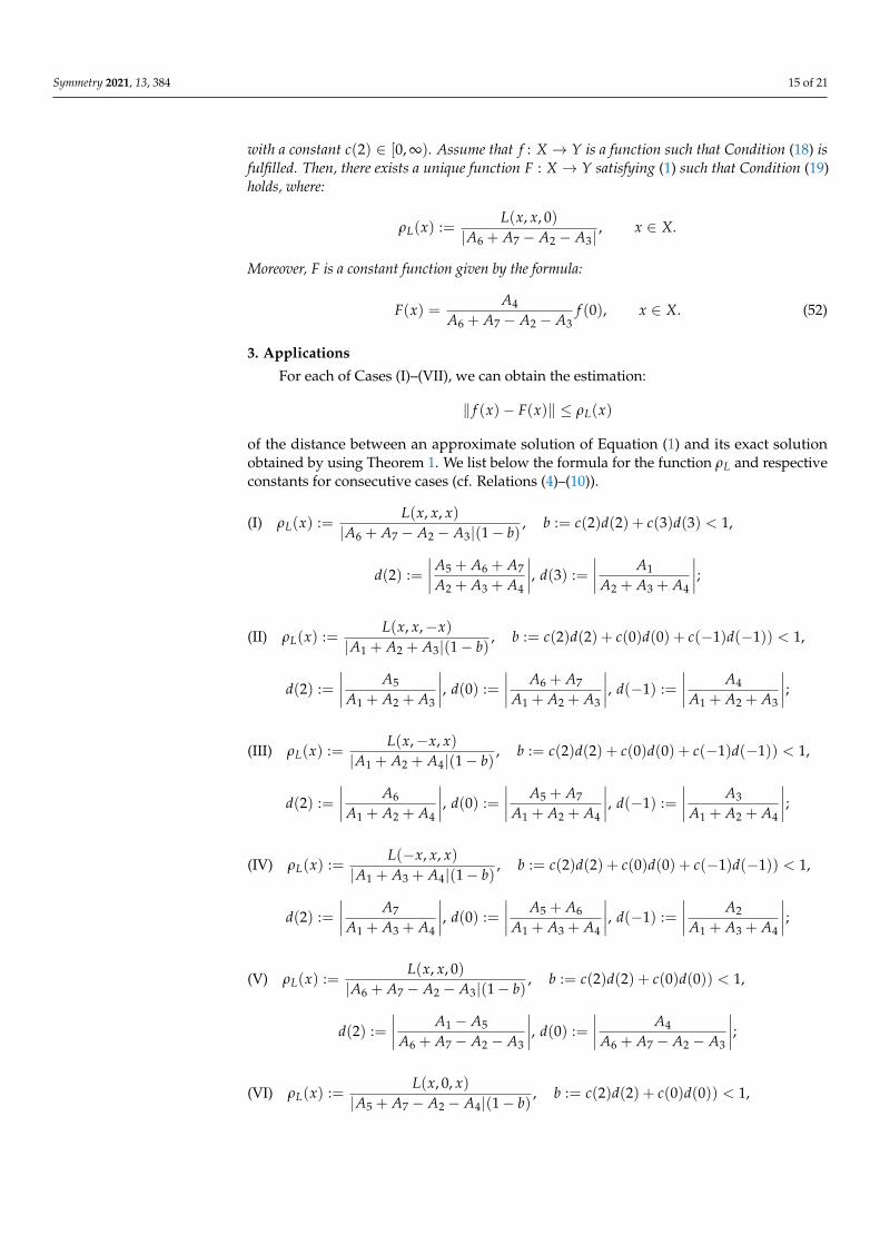
with a constant c(2) ∈ [0, ∞). Assume that f : X → Y is a function such that Condition (18) isfulfilled. Then, there exists a unique function F : X → Y satisfying (1) such that Condition (19)holds, where:

ρL(x) :=L(x, x, 0)

|A6 + A7 − A2 − A3|, x ∈ X.

Moreover, F is a constant function given by the formula:

F(x) =A4

A6 + A7 − A2 − A3f (0), x ∈ X. (52)

3. Applications

For each of Cases (I)–(VII), we can obtain the estimation:

‖ f (x)− F(x)‖ ≤ ρL(x)

of the distance between an approximate solution of Equation (1) and its exact solutionobtained by using Theorem 1. We list below the formula for the function ρL and respectiveconstants for consecutive cases (cf. Relations (4)–(10)).

(I) ρL(x) :=L(x, x, x)

|A6 + A7 − A2 − A3|(1− b), b := c(2)d(2) + c(3)d(3) < 1,

d(2) :=∣∣∣∣A5 + A6 + A7

A2 + A3 + A4

∣∣∣∣, d(3) :=∣∣∣∣ A1

A2 + A3 + A4

∣∣∣∣;(II) ρL(x) :=

L(x, x,−x)|A1 + A2 + A3|(1− b)

, b := c(2)d(2) + c(0)d(0) + c(−1)d(−1)) < 1,

d(2) :=∣∣∣∣ A5

A1 + A2 + A3

∣∣∣∣, d(0) :=∣∣∣∣ A6 + A7

A1 + A2 + A3

∣∣∣∣, d(−1) :=∣∣∣∣ A4

A1 + A2 + A3

∣∣∣∣;(III) ρL(x) :=

L(x,−x, x)|A1 + A2 + A4|(1− b)

, b := c(2)d(2) + c(0)d(0) + c(−1)d(−1)) < 1,

d(2) :=∣∣∣∣ A6

A1 + A2 + A4

∣∣∣∣, d(0) :=∣∣∣∣ A5 + A7

A1 + A2 + A4

∣∣∣∣, d(−1) :=∣∣∣∣ A3

A1 + A2 + A4

∣∣∣∣;(IV) ρL(x) :=

L(−x, x, x)|A1 + A3 + A4|(1− b)

, b := c(2)d(2) + c(0)d(0) + c(−1)d(−1)) < 1,

d(2) :=∣∣∣∣ A7

A1 + A3 + A4

∣∣∣∣, d(0) :=∣∣∣∣ A5 + A6

A1 + A3 + A4

∣∣∣∣, d(−1) :=∣∣∣∣ A2

A1 + A3 + A4

∣∣∣∣;(V) ρL(x) :=

L(x, x, 0)|A6 + A7 − A2 − A3|(1− b)

, b := c(2)d(2) + c(0)d(0)) < 1,

d(2) :=∣∣∣∣ A1 − A5

A6 + A7 − A2 − A3

∣∣∣∣, d(0) :=∣∣∣∣ A4

A6 + A7 − A2 − A3

∣∣∣∣;(VI) ρL(x) :=

L(x, 0, x)|A5 + A7 − A2 − A4|(1− b)

, b := c(2)d(2) + c(0)d(0)) < 1,

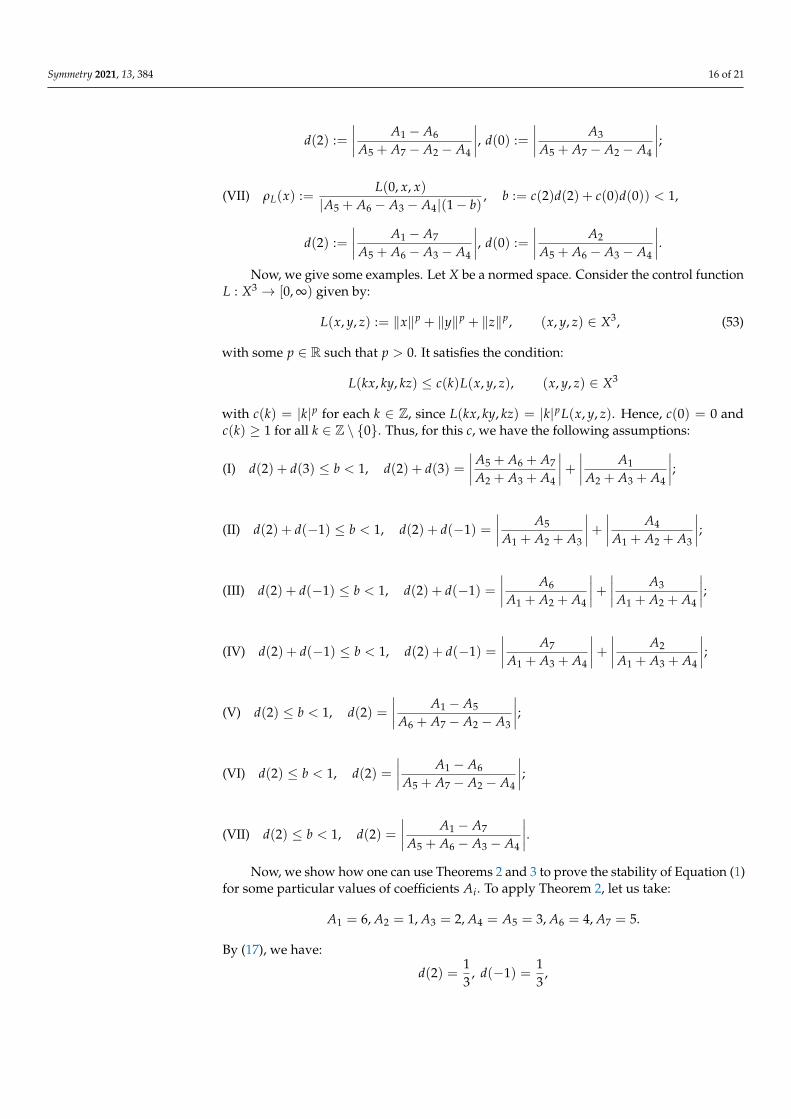
Symmetry 2021, 13, 384 16 of 21

d(2) :=∣∣∣∣ A1 − A6

A5 + A7 − A2 − A4

∣∣∣∣, d(0) :=∣∣∣∣ A3

A5 + A7 − A2 − A4

∣∣∣∣;(VII) ρL(x) :=

L(0, x, x)|A5 + A6 − A3 − A4|(1− b)

, b := c(2)d(2) + c(0)d(0)) < 1,

d(2) :=∣∣∣∣ A1 − A7

A5 + A6 − A3 − A4

∣∣∣∣, d(0) :=∣∣∣∣ A2

A5 + A6 − A3 − A4

∣∣∣∣.Now, we give some examples. Let X be a normed space. Consider the control function

L : X3 → [0, ∞) given by:

L(x, y, z) := ‖x‖p + ‖y‖p + ‖z‖p, (x, y, z) ∈ X3, (53)

with some p ∈ R such that p > 0. It satisfies the condition:

L(kx, ky, kz) ≤ c(k)L(x, y, z), (x, y, z) ∈ X3

with c(k) = |k|p for each k ∈ Z, since L(kx, ky, kz) = |k|pL(x, y, z). Hence, c(0) = 0 andc(k) ≥ 1 for all k ∈ Z \ {0}. Thus, for this c, we have the following assumptions:

(I) d(2) + d(3) ≤ b < 1, d(2) + d(3) =∣∣∣∣A5 + A6 + A7

A2 + A3 + A4

∣∣∣∣+ ∣∣∣∣ A1

A2 + A3 + A4

∣∣∣∣;(II) d(2) + d(−1) ≤ b < 1, d(2) + d(−1) =

∣∣∣∣ A5

A1 + A2 + A3

∣∣∣∣+ ∣∣∣∣ A4

A1 + A2 + A3

∣∣∣∣;(III) d(2) + d(−1) ≤ b < 1, d(2) + d(−1) =

∣∣∣∣ A6

A1 + A2 + A4

∣∣∣∣+ ∣∣∣∣ A3

A1 + A2 + A4

∣∣∣∣;(IV) d(2) + d(−1) ≤ b < 1, d(2) + d(−1) =

∣∣∣∣ A7

A1 + A3 + A4

∣∣∣∣+ ∣∣∣∣ A2

A1 + A3 + A4

∣∣∣∣;(V) d(2) ≤ b < 1, d(2) =

∣∣∣∣ A1 − A5

A6 + A7 − A2 − A3

∣∣∣∣;(VI) d(2) ≤ b < 1, d(2) =

∣∣∣∣ A1 − A6

A5 + A7 − A2 − A4

∣∣∣∣;(VII) d(2) ≤ b < 1, d(2) =

∣∣∣∣ A1 − A7

A5 + A6 − A3 − A4

∣∣∣∣.Now, we show how one can use Theorems 2 and 3 to prove the stability of Equation (1)

for some particular values of coefficients Ai. To apply Theorem 2, let us take:

A1 = 6, A2 = 1, A3 = 2, A4 = A5 = 3, A6 = 4, A7 = 5.

By (17), we have:

d(2) =13

, d(−1) =13

,

Symmetry 2021, 13, 384 17 of 21

whence by (34), we get that:

b = c(2)d(2) + c(−1)d(−1) =2p

3+

13

.

Consequently, b < 1 if and only if p ∈ (0, 1). In particular, for p = 12 , we have

b =√

2+13 and:

ρL(x) =L(x, x,−x)

9(1−√

2+13 )

=2 +√

22

√‖x‖.

Thus:

‖ f (x)− F(x)‖ ≤ 2 +√

22

√‖x‖,

where F is of the form:F(x) = a(x) + c, x ∈ X,

with an additive function a : X → Y and c = f (0).Let us note that we obtain the same approximate if, e.g., A6 = 100 and A7 = −91,

since the constant b occurring in Theorem 2 depends on |A6 + A7| and the values of A6and A7 taken into account separately have no effect on b.

To prove the stability of Equation (1) for these values of the coefficients, we can alsouse Theorem 3. Then, by (38) and (51), we have d(2) = 1

2 and:

b = c(2)d(2) =2p

2.

Consequently, b < 1 if and only if p ∈ (0, 1). In particular, for p = 12 , we have b =

√2

2 and:

ρL(x) =L(x, x, 0)

6(1−√

22 )

=2 +√

23

√‖x‖.

Thus:

‖ f (x)− F(x)‖ ≤ 2 +√

23

√‖x‖.

Summing up, for the considered values of coefficients, Theorem 3 gives a better approxi-mation than Theorem 2, since in the case p ∈ (0, 1), we have:

2p

2<

2p

3+

13

.

Now, let us take:

A1 = A2 = A3 = 2, A4 = A5 = A6 = A7 = 1.

First, we use Theorem 2. By (17), we have:

d(2) =16

, d(−1) =16

,

whence by (34), we get that:

b = c(2)d(2) + c(−1)d(−1) =2p

6+

16

.

Consequently, b < 1 if and only if p ∈ (0, log2 5). In particular, for p = 1, we haveb = 1

2 and:

ρL(x) =L(x, x,−x)

6(1− 12 )

=L(x, x,−x)

3= ‖x‖.

Symmetry 2021, 13, 384 18 of 21

For p = 12 , we have b =

√2+16 and:

ρL(x) =L(x, x,−x)

6(1−√

2+16 )

=L(x, x,−x)

5−√

2=

3(5 +√

2)23

√‖x‖ ≈ 0.8366

√‖x‖.

To prove the stability of Equation (1) for these values of the coefficients, we can alsouse Theorem 3. Then, by (38) and (51), we have d(2) = 1

2 and:

b = c(2)d(2) =2p

2.

Consequently, b < 1 if and only if p ∈ (0, 1). In particular, for p = 12 , we have b =

√2

2 and:

ρL(x) =L(x, x, 0)

2(1−√

22 )

= (2 +√

2)√‖x‖ ≈ 3.4142

√‖x‖.

Thus, now, Theorem 2 gives a better approximation than Theorem 3, since for p > 0,we have:

2p

6+

16<

2p

2.

Moreover, in this case, using Theorem 2, we obtain a wider interval for p.

4. Final Remarks

Let L : X3 → K satisfy:

L(kx, ky, kz) ≤ c(k)L(x, y, z), (x, y, z) ∈ X3

for some k ∈ Z. Define L : X3 → K by the formula:

L(x, y, z) := L(x, y, z) + δ,

where δ > 0. Then, if c(k) ≥ 1, then:

L(kx, ky, kz) = L(kx, ky, kz) + δ

≤ c(k)L(x, y, z) + δ

≤ c(k)(

L(x, y, z) +δ

c(k)

)≤ c(k)(L(x, y, z) + δ) = c(k)L(x, y, z).

Let L be given by (53). Then:

L(x, y, z) = ‖x‖p + ‖y‖p + ‖z‖p + δ, (x, y, z) ∈ X3. (54)

and the condition:

L(kx, ky, kz) ≤ c(k)L(x, y, z), (x, y, z) ∈ X3 (55)

holds for each k ∈ Z \ {0} with c(k) = |k|p. For k = 0, we have L(kx, ky, kz) = δ for all(x, y, z) ∈ X3. Hence, Relation (55) holds with c(0) = 1, since δ is the minimum of L. Thus,we obtain:

c(k) :={|k|p, if k 6= 0,1, if k = 0.

Let:A1 = A2 = A3 = 2, A4 = A5 = A6 = A7 = 1.

Symmetry 2021, 13, 384 19 of 21

By Theorem 2

b = c(2)d(2) + c(0)d(0) + c(−1)d(−1) =2p + 3

6.

Hence, b < 1 if and only if p ∈ (0, log2 3). For p = 1, we have b = 56 and:

ρL(x) =L(x, x,−x)

6(1− 56 )

= L(x, x,−x) = 3‖x‖p + δ.

Now, let A2 = A3 = 2, A1 = A4 = A5 = A6 = A7 = 1. By Theorem 2,b = 2p+3

5 , since:

d(2) =15

, d(0) =25

, d(−1) =15

.

Then, b < 1 if and only if p ∈ (0, 1). In particular, for p = 12 , we obtain:

b =3 +√

25

, ρL(x) =L(x, x,−x)

5(1− 3+√

25 )

=3√‖x‖+ δ

2−√

2=

2 +√

22

(3√‖x‖+ δ

).

By Theorem 3 with the same constants as above, we get that b = 12 , and b < 1 if and only if

p ∈ (0, ∞), because d(2) = 0, d(0) = 12 . The estimate is:

ρL(x) =L(x, x, 0)2(1− 1

2 )= 2‖x‖p + δ.

For p = 12 , we have b = 1

2 , and ρL(x) = 2√‖x‖+ δ.

5. Discussion

In order to obtain a solution of a generalized Fréchet functional equation, we usedthe iterative method based on a fixed point theorem. The distance between the obtainedexact solution and the approximate solution being the starting point of the iterative processdepends on the length of the first step of this process and the parameter b controlling thelength of the subsequent steps. The choice of the operator generating the iterative sequencetending to the exact solution has a big impact on the accuracy of the estimation of thedistance between this solution and the initial approximate solution.

In this paper, we distinguished seven cases depending on the conditions met by thecoefficients of the generalized Fréchet equation having constant coefficients. The result forthe first of these cases was presented in [10]. It gives a good estimate for some values ofthe coefficients of the considered equation. However, for other values of the coefficients,these estimates may not be very accurate. Therefore, we distinguished other cases in orderto compare the obtained estimates. For each of these cases, we provided an estimate of thedistance between the exact and approximate solutions of the generalized Fréchet equation.For the given values of the coefficients of the equation, we can choose the case that givesa good estimate after checking if its assumptions are met. In particular, we showed anexample of the coefficients for which Theorem 2 gives a better estimate than Theorem 3and an example where Theorem 3 gives a more accurate result.

The system of linear equations defining the list of cases was selected so that, on the onehand, for any values of the coefficients, at least one of the cases was satisfied, and on theother hand, the operator defining the iterative sequence did not have too many summands.One can try to use such a system for a generalized Fréchet functional equation with variablecoefficients, but then, it may happen that an equation of the system is satisfied for somevalues of x, y, and z, and for others, it does not hold.

Symmetry 2021, 13, 384 20 of 21

6. Conclusions

In this paper, we study the dependence of an estimation of the distance betweenapproximate and exact solutions of the generalized Fréchet functional equation from thevalues of coefficients Ai of this equation. We distinguish seven cases, of which at least one isalways true. However, usually more than one of these cases holds, and then, we can choosethe one that gives the best estimate among them. Generally speaking, we try to group thecoefficients of the equation in a way that gives a good estimation of the distance betweenthe approximate and exact solutions. The division into groups is important because withinthe groups, we sum up directly the coefficients and not their absolute values.

The desired estimate depends not only on the coefficients of the equation, but alsoon the control function L, as we showed in the examples. Nevertheless, grouping thecoefficients may also be useful in investigating the stability of more general functionalequations than the equation discussed in this article.

Author Contributions: Conceptualization, J.B.; methodology, J.B., Z.L., and R.M.; investigation,J.B., Z.L., and R.M.; writing, original draft preparation, R.M.; writing, review and editing, Z.L.;supervision, J.B. All authors read and agreed to the published version of the manuscript.

Funding: This research received no external funding.

Institutional Review Board Statement: Not applicable.

Informed Consent Statement: Not applicable.

Data Availability Statement: Not applicable.

Conflicts of Interest: The authors declare no conflict of interest.

References1. Fréchet, M. Sur la définition axiomatique d’une classe d’espaces vectoriels distanciés applicables vectoriellement sur l’espace de

Hilbert. Ann. Math. 1935, 36, 705–718. [CrossRef]2. Alsina, C.; Sikorska, J.; Tomás, M.S. Norm Derivatives and Characterizations of Inner Product Spaces; World Scientific Publishing Co.:

Singapore, 2010.3. Bahyrycz, A.; Brzdek, J.; Piszczek, M.; Sikorska, J. Hyperstability of the Fréchet equation and a characterization of inner product

spaces. J. Funct. Spaces Appl. 2013, 2013, 496361. [CrossRef]4. Dragomir, S.S. Some characterizations of inner product spaces and applications. Studia Univ. Babes-Bolyai Math. 1989, 34, 50–55.5. Jordan, P.; von Neumann, J. On inner products in linear, metric spaces. Ann. Math. 1935, 36, 719–723. [CrossRef]6. Moslehian, M.S.; Rassias, J.M. A Characterization of Inner Product Spaces Concerning an Euler-Lagrange Identity. Commun.

Math. Anal. 2010, 8, 16–21.7. Nikodem, K.; Páles, Z. Characterizations of inner product spaces by strongly convex functions. Banach J. Math. Anal. 2011, 5,

83–87. [CrossRef]8. Rassias, T.M. New characterizations of inner product spaces. Bull. Sci. Math. 1984, 108, 95–99.9. Bahyrycz, A.; Brzdek, J.; Jabłonska, E.; Malejki, R. Ulam’s stability of a generalization of the Fréchet functional equation. J. Math.

Anal. Appl. 2016, 442, 537–553. [CrossRef]10. Brzdek, J.; Lesniak, Z.; Malejki, R. On the generalized Fréchet functional equation with constant coefficients and its stability.

Aequationes Math. 2018, 92, 355–373. [CrossRef]11. Malejki, R. Stability of a generalization of the Fréchet functional equation. Ann. Univ. Paedagog. Crac. Stud. Math. 2015, 14, 69–79.

[CrossRef]12. Hyers, D.H.; Isac, G.; Rassias, T.M. Stability of Functional Equations in Several Variables; Birkhäuser: Boston, MA, USA, 1998.13. Jung, S.-M. Hyers-Ulam-Rassias Stability of Functional Equations in Nonlinear Analysis; Springer Optimization and Its Applications;

Springer: New York, NY, USA, 2011; Volume 48.14. Kannappan, P. Functional Equations and Inequalities with Applications; Springer Monographs in Mathematics; Springer: New York,

NY, USA, 2009.15. Brillouët-Belluot, N.; Brzdek, J.; Cieplinski, K. On some recent developments in Ulam’s type stability. Abstr. Appl. Anal. 2012,

2012, 716936. [CrossRef]16. Brzdek, J.; Cieplinski, K.; Lesniak, Z. On Ulam’s type stability of the linear equation and related issues. Discret. Dyn. Nat. Soc.

2014, 2014, 536791. [CrossRef]17. Jung, S.-M. On the Hyers-Ulam stability of the functional equation that have the quadratic property. J. Math. Anal. Appl. 1998,

222, 126–137. [CrossRef]18. Brzdek, J. Remarks on hyperstability of the Cauchy functional equation. Aequationes Math. 2013, 86, 255–267. [CrossRef]

Symmetry 2021, 13, 384 21 of 21

19. Brzdek, J.; Jabłonska, E.; Moslehian, M.S.; Pacho, P. On stability of a functional equation of quadratic type. Acta Math. Hungar.2016, 149, 160–169.

20. Fechner, W. On the Hyers-Ulam stability of functional equations connected with additive and quadratic mappings. J. Math. Anal.Appl. 2006, 322, 774–786. [CrossRef]

21. Gselmann, E. Hyperstability of a functional equation. Acta Math. Hungar. 2009, 124, 179–188. [CrossRef]22. Lee, Y.-H. On the Hyers-Ulam-Rassias stability of the generalized polynomial function of degree 2. J. Chuncheong Math. Soc. 2009,

22, 201–209.23. Maksa, G.; Páles, Z. Hyperstability of a class of linear functional equations. Acta Math. Acad. Paedag. Nyìregyháziensis 2001, 17,

107–112.24. Phochai, T.; Saejung, S. Hyperstability of generalised linear functional equations in several variables. Bull. Aust. Math. Soc. 2020,

102, 293–302. [CrossRef]25. Piszczek, M. Remark on hyperstability of the general linear equation. Aequationes Math. 2014, 88, 163–168. [CrossRef]26. Popa, D.; Rasa, I. The Fréchet functional equation with application to the stability of certain operators. J. Approx. Theory 2012, 164,

138–144. [CrossRef]27. Sikorska, J. On a direct method for proving the Hyers-Ulam stability of functional equations. J. Math. Anal. Appl. 2010, 372,

99–109. [CrossRef]28. Brzdek, J. Hyperstability of the Cauchy equation on restricted domains. Acta Math. Hung. 2013, 141, 58–67. [CrossRef]29. Bahyrycz, A.; Olko, J. On stability of the general linear equation. Aequationes Math. 2015, 89, 1461–1474. [CrossRef]30. Bahyrycz, A.; Olko, J. Hyperstability of general linear equation. Aequationes Math. 2016, 90, 527–540. [CrossRef]31. Zhang, D. On Hyers-Ulam stability of generalized linear functional equation and its induced Hyers-Ulam programming problem.

Aequat. Math. 2016, 90, 559–568. [CrossRef]32. Zhang, D. On hyperstability of generalised linear functional equations in several variables. Bull. Aust. Math. Soc. 2015, 92,

259–267. [CrossRef]33. Badora, R.; Brzdek, J. Fixed points of a mapping and Hyers-Ulam stability. J. Math. Anal. Appl. 2014, 413, 450–457. [CrossRef]34. Bahyrycz, A.; Brzdek, J.; Lesniak, Z. On approximate solutions of the generalized Volterra integral equation. Nonlinear Anal. Real

World Appl. 2014, 20, 59–66. [CrossRef]35. Brzdek, J.; Cieplinski, K. A fixed point approach to the stability of functional equations in non-Archimedean metric spaces.

Nonlinear Anal. 2011, 74, 6861–6867. [CrossRef]36. Cadariu, L.; Gavruta, L.; Gavruta, P. Fixed points and generalized Hyers-Ulam stability. Abstr. Appl. Anal. 2012, 2012, 712743.

[CrossRef]37. Brzdek, J.; Chudziak, J.; Páles, Z. A fixed point approach to stability of functional equations. Nonlinear Anal. 2011, 74, 6728–6732.

[CrossRef]