arX

iv:g

r-qc

/020

4053

v2 2

4 Ju

n 20

02

ICN-UNAM-02-02gr-qc/0204053

On Unitary Time Evolution in Gowdy T 3 Cosmologies

Alejandro Corichi1,2∗, Jeronimo Cortez1 and Hernando Quevedo1

1. Instituto de Ciencias Nucleares

Universidad Nacional Autonoma de Mexico

A. Postal 70-543, Mexico D.F. 04510, MEXICO

2. Department of Physics and Astronomy

University of Mississippi, University, MS 38677, USA

Abstract

A non-perturbative canonical quantization of Gowdy T 3 polarized models

carried out recently is considered. This approach profits from the equivalence

between the symmetry reduced model and 2+1 gravity coupled to a massless

real scalar field. The system is partially gauge fixed and a choice of internal

time is performed, for which the true degrees of freedom of the model reduce

to a massless free scalar field propagating on a 2-dimensional expanding torus.

It is shown that the symplectic transformation that determines the classical

dynamics cannot be unitarily implemented on the corresponding Hilbert space

of quantum states. The implications of this result for both quantization of

fields on curved manifolds and physically relevant questions regarding the

initial singularity are discussed.

Pacs: 04.60.Ds, 04.60.Kz, 04.62.+v

Typeset using REVTEX

∗Email: corichi, cortez, quevedo@nuclecu.unam.mx

1

I. INTRODUCTION

In the search for a quantum theory of gravity within the canonical approach, it has beenhistorically useful to consider symmetry reduced models. The most studied examples arehomogeneous models, where the infinite dimensional system is reduced to a model with afinite number of degrees of freedom. These are known as mini-superspace models [1]. An-other class of symmetry reduced models where the resulting system is still a field theorywith an infinite number of degrees of freedom are known as midi-superspace models (fora recent review see [2]). Recently, within this class, the models that have received specialattention are the Einstein-Rosen waves and Gowdy cosmological models [3–5]. One inter-esting feature of this type of models is that due to their spacetime symmetries, the classicaldynamics turns out to be derivable from an equivalent complete integrable system, but theystill possess an infinite number of degrees of freedom so that their quantization would leadto a true quantum field theory (in contrast to mini-superspace models with a finite numberof degrees of freedom). In this work, we will consider the canonical quantization of thepolarized Gowdy T 3 cosmological model [6]. This is the simplest inhomogeneous, empty,spatially closed cosmological model. It was extensively studied in the 70’s [7,8], and subse-quently re-examined by several authors [9,10]. Of particular relevance is the recent work byPierri, where definite progress was achieved in defining a rigorous quantization of the model[4]. In this case, the quantization is based on the fact that the corresponding gravitationalfield can be equivalently treated as 2 + 1 gravity coupled to a massless scalar field, definedon a 2 + 1-dimensional manifold with topology T 2 × R.

One important aspect in the study of quantum cosmological models is dynamical evolu-tion; that is the dynamics in which a physical quantum state evolves from an initial Cauchysurface to a final one. Recall that in general relativity there are no preferred foliations inspacetime and the dynamical evolution should consider all possible spacelike foliations inorder to be in agreement with the requirement of general covariance. Furthermore, in thecase in which the Cauchy surfaces are compact, dynamical evolution is pure gauge, so anyinterpretation of time evolution is normally through a deparametrization procedure which,in the Hamiltonian language, is normally achieved via “time dependent gauge fixing”. Thus,the dynamics to be considered in quantum cosmological models concerns the evolution ofquantum states between Cauchy surfaces, defined by the particular gauge choice. Differentchoices of time parameters may lead to inequivalent quantizations. This fact is true even inthe simple mechanical mini-superspace models. In the particular model we are interested,the system is partially gauge fixed at the classical level, and in particular a time function Tis chosen and interpreted as the time which defines “evolution”. The surfaces of constant Tare Cauchy surfaces of a fiducial flat background, so the model get reduced to a quantumscalar field on a flat background, equipped with a foliation of preferred surfaces which define“time evolution” in the corresponding quantum gravitational system.

At the classical level, this dynamical evolution of the field can be represented as a canon-ical transformation that acts on points of the corresponding phase space. The question iswhether, at the quantum level, this canonical transformation can be implemented on thespace of quantum states of the field by means of a unitary operator. This is a rather delicateproblem that has been analyzed in detail only recently and for a few special cases [11–14],all of them concerning free scalar fields on flat or stationary spacetimes. Fortunately, the

2

quantum polarized Gowdy T 3 cosmological models belong to this class, and so we will beable to investigate the question about the unitary implementability of these models withinthis approach. This is the main goal of the present work.

We will show that for the particular quantization performed in [4,5], time evolution is notimplementable as a unitary evolution. Given that, at the classical level time evolution is puregauge, and the particular choice of time is an ad-hock procedure to regain dynamics from apurely frozen formalism, one might argue that unitary implementability of this fictitious timeevolution is not necessary for the consistency of the formalism. However, as we will argue,the implementability is needed in order to ask physically meaningful questions regarding,say, the initial singularity. That is, questions such as whether the initial singularity issmeared by quantum effects should have a definite answer within a consistent quantization.Thus, we shall conclude that we can not extract any physics out of these models as presentlyconstructed.

This paper is organized as follows. In Sec. II we review the quantization of polarizedGowdy T 3 cosmological models as performed by Pierri [4,5]. We show that the two differentsets of creation and annihilation operators proposed in this quantization are related bymeans of a unitary Bogoliubov transformation. In Sec. IIIA we explicitly calculate thecanonical (symplectic) transformation that represents the classical evolution of the system.In Sec. III B we prove that this canonical transformation is not unitarily implementable onthe corresponding Fock space. We end with a discussion and some conclusions in Sec. IV.

II. CANONICAL QUANTIZATION

The polarized Gowdy T 3 models are globally hyperbolic four-dimensional vacuum space-times, with two commuting hypersurface orthogonal spacelike Killing fields and compactspacelike hypersurfaces homeomorphic to a three-torus. Because this system can be equiv-alent treated as 2+1 gravity (minimally) coupled to an axi-symmetric massless scalar field,let us begin by considering the action

S[ (3)g, ψ ] =1

2π

∫

(3)Md3x

√

−(3)g ((3)R− (3)gab∇aψ∇bψ) (1)

where (3)R is the Ricci scalar of the 3-d spacetime ((3)M,(3) gab),(3)M is a 3-d manifold with

topology T 2 × R and spacetime metric (3)gab = hab + τ 2∇aσ∇bσ. The Killing field σa ishypersurface orthogonal and the field hab is a metric of signature (−,+) on the 2-manifoldorthogonal to σa; τ is the norm of σa and σ is an angular coordinate with range 0 ≤ σ < 2πsuch that σa∇aσ = 1.

Introducing a generic slicing by compact spacelike hypersurfaces labeled by t = const the2-metric can be written as hab = (−N2 +N θNθ)∇at∇bt+ 2Nθ∇(at∇b)θ + eγ∇aθ∇bθ, wherethe lapse, N , the shift, N θ, and γ are functions of θ and t. The angular coordinate θ ∈ [0, 2π)is such that θa∇aθ = 1, where θa is the unit vector field within each slice orthogonal to σa.Thus the system consists of five functions (N, N θ, γ, τ, ψ) of t and θ which are periodicin θ. The function ψ represents the zero rest mass scalar field.

Substituting the expression for (3)gab in the action (1) we pass to the Hamiltonian for-mulation

3

S =∫

dt(∮

(pγ γ + pτ τ + pψψ))

−H [N,N θ] (2)

where the HamiltonianH is given by H [N,N θ] =∮

(NC+N θCθ) (here, the symbol∮

denotesintegration over θ ∈ S1) and the first class constraints C and Cθ are

C = e−γ/2[

2τ ′′ − γ′τ ′ − pγpτ + τ( p2

ψ

4τ 2+ ψ′2

)]

(3)

Cθ = e−γ(γ′pγ − 2p′γ + τ ′pτ + pψψ′) (4)

The lapse and shift are not dynamical variables, thus the phase space Γ consists of threecanonically-conjugate pairs of periodic functions of θ, (γ, pγ; τ, pτ ;ψ, pψ) on a 2-d manifoldΣ with topology T 2.

Because the Hamiltonian vanishes on the constraint surface there is no distinction be-tween gauge and dynamics and therefore it is necessary to introduce a “deparametrization”procedure to discuss dynamics. From the infinite set of vector fields generated by the Hamil-tonian constraints we select one to represent evolution and gauge fix the others. For gaugefixing let us demand

pγ + p = 0 and τ(θ)′ = 0 (5)

where p is a spatial constant that has zero Poisson bracket with all the constraints and henceit can not be removed by gauge fixing. The second condition will allow us to regard τ(θ) asthe time parameter.

The consistency of the formalism requires that the Poisson brackets τ(θ)′, H [N,N θ]and pγ + p,H [N,N θ] vanish. This can be achieved if the freely specifiable N and N θ arechosen as,

N =eγ/2

pand N θ = 0 (6)

therefore the coordinate condition (5) is acceptable. Indeed, for the special choice (6) wehave that τ(θ) = 1 and pγ(θ) = −p = 0 and hence p becomes a true constant that can beassociated with a time scaling parameter in the original 3+1-spacetime. Thus, apart froma global degree of freedom, the true degrees of freedom will all reside in the field ψ. Solvingthe set of second class constraints (C,Cθ, pγ + p, τ ′) the result is

pτ = − t

p

( p2ψ

4t2+ ψ′2

)

(7)

γ(θ) =1

p

∫ θ

0dθ1pψψ

′ + γ(0) (8)

Since γ is a smooth function of θ, it must admit a Fourier series of the form γ = q +∑

n 6=0einθ√

2πγn, then

∑

n 6=0(einθ−1√

2π)γn = 1

p

∫ θ0 dθ1pψψ

′ and we can solve for all modes but the zero

mode. i.e., we can solve (8) for γ :=∑

n 6=0einθ√

2πγn and we are left with the global degree of

4

freedom q = 12π

∮

γ unsolved. This is consistent with the fact that a constant shift vectorN θ = const would also be acceptable for preserving the conditions (5). Substituting (8) in(6) we obtain that N = N [q, p, ψ, pψ]. The spacetime metric is now completely determinedby q, p, ψ and pψ

(3)gab = eq+γ(

− 1

p2∇at∇bt+ ∇aθ∇bθ

)

+ t2∇aσ∇bσ (9)

The phase space variables are periodic functions of θ, therefore γ(2π)− γ(0) = 0 defines viaEq.(8) the global constraint

Pθ :=∮

pψ ψ′ = 0 (10)

The non-degenerate symplectic structure on the reduced phase space Γr = Γg⊕ Γ, whereΓg is coordinatized by the pair (q, p) and Γ by (ψ, pψ), is the pull-back of the naturalsymplectic structure defined on Γ. Thus q, p = 1 and ψ(θ1), pψ(θ2) = δ(θ1, θ2) on Γr.

Substituting (5) and (7) in (2) we obtain the reduced action

S =∫

dt

(

pq +∮[

pψψ − t

p

(

p2ψ

4t2+ ψ′2

)

]

)

(11)

and the reduced Hamiltonian

H =∮

t

p

[

p2ψ

4t2+ ψ′2

]

(12)

Varying the action (11) with respect to ψ and pψ, the field equations are ∂ψ∂T

=pψ2Tp

and∂pψ∂T

=2Tpψ′′, which is equivalent to the Klein-Gordon equation for the scalar field ψ propagatingon a fictitious flat background (f)gab = −∇aT∇bT + ∇aθ∇bθ + T 2∇aσ∇bσ, with the furtherrestriction that the field ψ does not depend on σ. Here the constant rescaling T := t/phas been considered, in order to simplify the resulting dynamical equation for ψ. Hence thephase space Γ, coordinatized by ϕ := ψ(θ) and π := pψ(θ), corresponds to the symplecticvector space (V,ΩV ) of smooth real solutions to the Klein-Gordon equation (f)gab∇a∇bψ = 0,where the symplectic structure ΩV is given by

ΩV (ψ1, ψ2) =∮

T (ψ2∂Tψ1 − ψ1∂Tψ2) (13)

Note that the choice of internal time T : Γ 7→ R, depends on the point of phase space,in particular, on the global degree of freedom p, making it a q−number. Recall that in thiscase, one has deparametrized the system, that is, one has defined a fictitious time evolutionwith respect to the number t. Strictly speaking, from the canonical viewpoint one shouldchoose a particular value t0 of the time parameter in order to fix once and for all a singleCauchy surface Σ0. This would be the “frozen formalism” description, where only the truedegrees of freedom are left and the notion of dynamics has been lost. However, for thepurposes of quantization, it is convenient to exploit this deparametrization since this allowsto complete the quantization in a rigorous fashion. However, in the quantum theory the

5

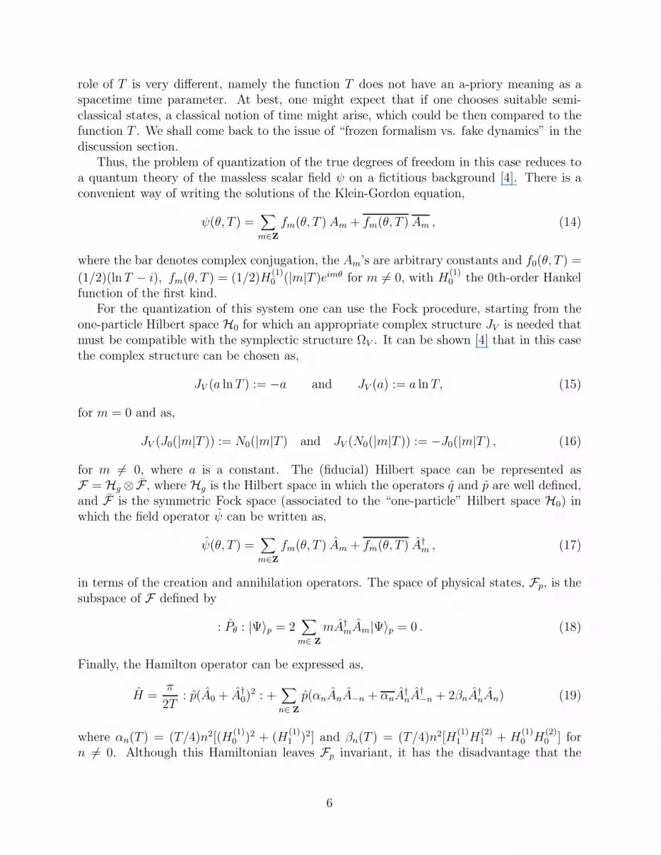
role of T is very different, namely the function T does not have an a-priory meaning as aspacetime time parameter. At best, one might expect that if one chooses suitable semi-classical states, a classical notion of time might arise, which could be then compared to thefunction T . We shall come back to the issue of “frozen formalism vs. fake dynamics” in thediscussion section.

Thus, the problem of quantization of the true degrees of freedom in this case reduces toa quantum theory of the massless scalar field ψ on a fictitious background [4]. There is aconvenient way of writing the solutions of the Klein-Gordon equation,

ψ(θ, T ) =∑

m∈Z

fm(θ, T ) Am + fm(θ, T ) Am , (14)

where the bar denotes complex conjugation, the Am’s are arbitrary constants and f0(θ, T ) =

(1/2)(lnT − i), fm(θ, T ) = (1/2)H(1)0 (|m|T )eimθ for m 6= 0, with H

(1)0 the 0th-order Hankel

function of the first kind.For the quantization of this system one can use the Fock procedure, starting from the

one-particle Hilbert space H0 for which an appropriate complex structure JV is needed thatmust be compatible with the symplectic structure ΩV . It can be shown [4] that in this casethe complex structure can be chosen as,

JV (a lnT ) := −a and JV (a) := a lnT, (15)

for m = 0 and as,

JV (J0(|m|T )) := N0(|m|T ) and JV (N0(|m|T )) := −J0(|m|T ) , (16)

for m 6= 0, where a is a constant. The (fiducial) Hilbert space can be represented asF = Hg ⊗ F , where Hg is the Hilbert space in which the operators q and p are well defined,and F is the symmetric Fock space (associated to the “one-particle” Hilbert space H0) inwhich the field operator ψ can be written as,

ψ(θ, T ) =∑

m∈Z

fm(θ, T ) Am + fm(θ, T ) A†m , (17)

in terms of the creation and annihilation operators. The space of physical states, Fp, is thesubspace of F defined by

: Pθ : |Ψ〉p = 2∑

m∈ Z

mA†mAm|Ψ〉p = 0 . (18)

Finally, the Hamilton operator can be expressed as,

H =π

2T: p(A0 + A†

0)2 : +

∑

n∈ Z

p(αnAnA−n + αnA†nA

†−n + 2βnA

†nAn) (19)

where αn(T ) = (T/4)n2[(H(1)0 )2 + (H

(1)1 )2] and βn(T ) = (T/4)n2[H

(1)1 H

(2)1 + H

(1)0 H

(2)0 ] for

n 6= 0. Although this Hamiltonian leaves Fp invariant, it has the disadvantage that the

6

vacuum state is not an eigenvector of it with zero eigenvalue. In order to avoid this difficulty,a new set of creation and annihilation operators has been recently proposed [5]:

a0 =i√2(√

3A0 + A†0), (20)

and

an =

√

π

2(αnAn + βnA

†−n) , (21)

where αn = αn/(|n|βn) and βn =√

(βn − |n|/π)/|n|. It should be noted that our choice

differs from that in [5], which does not satisfy the relations [an, a†n′] = δn,n′. In this new set

the Hamilton operator can be written as,

: H :=1

Tp P 2

0 +2

π

∑

n∈Z

|n| p a†nan , (22)

with P0 = i√π/(1 +

√3)(a†0 − a0). For this Hamiltonian, the vacuum state is in fact an

eigenvector with zero eigenvalue. The question arises whether locally the two different setsof creation and annihilation operators lead to different quantizations. If so, one would needto investigate the problem of unitary implementability (to be treated in the next section) forboth sets separately. To answer this question we have analyzed the coefficients that relatethe old operators An with the new ones an. A straightforward calculation shows that theysatisfy the relationships,

∑

k

(αmkαnk − βmkβnk) = δm,n , (23)

and∑

k

(αmkβnk − βmkαnk) = 0 , (24)

where αmk = αmδm,k and βmk = βmδ−m,k. Moreover, the coefficients βmk are square-summable. To see this, let C(|m|T ) = (βm − |m|/π)/|m| and let N be a positive integersuch that NT >> 1, then

∑

m,n

|βnm|2 =∑

m

|βm|2 = 2N−1∑

m=1

C(mT ) + 2∞∑

m=N

C(mT ) (25)

and the condition that the coefficients βmk are square-summable is equivalent to

∞∑

m=N

C(mT ) <∞ (26)

Now, from the expansions for Jn(x) and Nn(x) [19]; i.e.,

Jn(x) =

√

2

πx

[

Pn(x) cos

(

x− (n+ 12)π

2

)

−Qn(x) sin

(

x− (n + 12)π

2

)]

, (27)

Nn(x) =

√

2

πx

[

Pn(x) sin

(

x− (n+ 12)π

2

)

+Qn(x) cos

(

x− (n + 12)π

2

)]

,

7

where

Pn(x) = 1 − (4n2 − 1)(4n2 − 9)

2!(8x)2+

(4n2 − 1)(4n2 − 9)(4n2 − 25)(4n2 − 49)

4!(8x)4− . . . , (28)

Qn(x) =(4n2 − 1)

1!(8x)− (4n2 − 1)(4n2 − 9)(4n2 − 25)

3!(8x)3+ . . . ,

it is easy to see that

C(kT ) =Tk

4

[

2

πTk(P 2

1 (kT ) + P 20 (kT ) +Q2

1(kT ) +Q20(kT ))

]

− 1

π. (29)

That is, for kT >> 1 we obtain that

C(kT ) =Tk

4

[

2

πTk(2 +O(1/(kT )2))

]

− 1

π(30)

where O(1/(kT )2) contains all the terms of the form ci(kT )n

, with ci some (real) constants

and N ∋ n ≥ 2. Because∑

kci

(kT )nconverges (the Riemann zeta function defined by

ζ(p) =∑∞k=1 k

−p is divergent for p ≤ 1 and convergent for p > 1) then Eq. (30) impliesEq. (26) and therefore the coefficients βmk are square-summable. Thus, the transformationbetween the two different sets of creation and annihilation operators is a unitary Bogoliubovtransformation [15,17]. Consequently, the second set of operators, an, corresponds only tothe choice of a second complete set of modes fn. Thus, we can equivalently choose anyof these two sets of creation and annihilation operators given above. We will perform theanalysis of the quantum implementability of the classical dynamical evolution in Sec. III,using the operators An and the complex structure given above.

III. FUNCTIONAL EVOLUTION

It is known that for a massless, free, real scalar field propagating on a (n+1)-dimensionalstatic spacetime with topology T n × R, dynamical evolution along arbitrary spacelike fo-liations is unitarily implemented on the same Fock space as that associated with inertialfoliations if n = 1 [13] and will not be, in general, unitarily implemented if n > 1 [14].However, for the (special) case in which we consider time evolution of the Klein-Gordonfield between any two flat spacelike Cauchy surfaces, dynamical evolution is unitarily imple-mentable for all positive integers n. In this section we will see that this result actually doesnot extend to our case, where the spatial slices have the same topology (tori) but now theyare expanding.

A. The symplectic transformation of classical dynamics

It is generally known that the phase space of a real, linear Klein-Gordon field propagatingon a globally hyperbolic background spacetime (M ≃ Σ×R, gab) with Σ a compact spacelikeCauchy surface, can be alternatively described by the space Γ of Cauchy data, that is

8

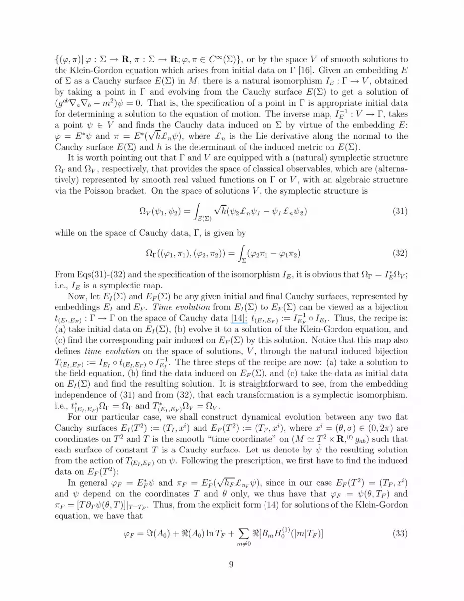
(ϕ, π)|ϕ : Σ → R, π : Σ → R;ϕ, π ∈ C∞(Σ), or by the space V of smooth solutions tothe Klein-Gordon equation which arises from initial data on Γ [16]. Given an embedding Eof Σ as a Cauchy surface E(Σ) in M , there is a natural isomorphism IE : Γ → V , obtainedby taking a point in Γ and evolving from the Cauchy surface E(Σ) to get a solution of(gab∇a∇b −m2)ψ = 0. That is, the specification of a point in Γ is appropriate initial datafor determining a solution to the equation of motion. The inverse map, I−1

E : V → Γ, takesa point ψ ∈ V and finds the Cauchy data induced on Σ by virtue of the embedding E:ϕ = E∗ψ and π = E∗(

√h£nψ), where £n is the Lie derivative along the normal to the

Cauchy surface E(Σ) and h is the determinant of the induced metric on E(Σ).It is worth pointing out that Γ and V are equipped with a (natural) symplectic structure

ΩΓ and ΩV , respectively, that provides the space of classical observables, which are (alterna-tively) represented by smooth real valued functions on Γ or V , with an algebraic structurevia the Poisson bracket. On the space of solutions V , the symplectic structure is

ΩV (ψ1, ψ2) =∫

E(Σ)

√h(ψ2£nψ1 − ψ1£nψ2 ) (31)

while on the space of Cauchy data, Γ, is given by

ΩΓ((ϕ1, π1), (ϕ2, π2)) =∫

Σ(ϕ2π1 − ϕ1π2) (32)

From Eqs(31)-(32) and the specification of the isomorphism IE , it is obvious that ΩΓ = I∗EΩV ;i.e., IE is a symplectic map.

Now, let EI(Σ) and EF (Σ) be any given initial and final Cauchy surfaces, represented byembeddings EI and EF . Time evolution from EI(Σ) to EF (Σ) can be viewed as a bijectiont(EI ,EF ) : Γ → Γ on the space of Cauchy data [14]: t(EI ,EF ) := I−1

EF IEI . Thus, the recipe is:

(a) take initial data on EI(Σ), (b) evolve it to a solution of the Klein-Gordon equation, and(c) find the corresponding pair induced on EF (Σ) by this solution. Notice that this map alsodefines time evolution on the space of solutions, V , through the natural induced bijectionT(EI ,EF ) := IEI t(EI ,EF ) I−1

EI. The three steps of the recipe are now: (a) take a solution to

the field equation, (b) find the data induced on EF (Σ), and (c) take the data as initial dataon EI(Σ) and find the resulting solution. It is straightforward to see, from the embeddingindependence of (31) and from (32), that each transformation is a symplectic isomorphism.i.e., t∗(EI ,EF )ΩΓ = ΩΓ and T ∗

(EI ,EF )ΩV = ΩV .For our particular case, we shall construct dynamical evolution between any two flat

Cauchy surfaces EI(T2) := (TI , x

i) and EF (T 2) := (TF , xi), where xi = (θ, σ) ∈ (0, 2π) are

coordinates on T 2 and T is the smooth “time coordinate” on (M ≃ T 2 ×R,(f) gab) such thateach surface of constant T is a Cauchy surface. Let us denote by ψ the resulting solutionfrom the action of T(EI ,EF ) on ψ. Following the prescription, we first have to find the induceddata on EF (T 2):

In general ϕF = E∗Fψ and πF = E∗

F (√hF£nF

ψ), since in our case EF (T 2) = (TF , xi)

and ψ depend on the coordinates T and θ only, we thus have that ϕF = ψ(θ, TF ) andπF = [T∂Tψ(θ, T )]|T=TF . Thus, from the explicit form (14) for solutions of the Klein-Gordonequation, we have that

ϕF = ℑ(A0) + ℜ(A0) lnTF +∑

m6=0

ℜ[BmH(1)0 (|m|TF )] (33)

9

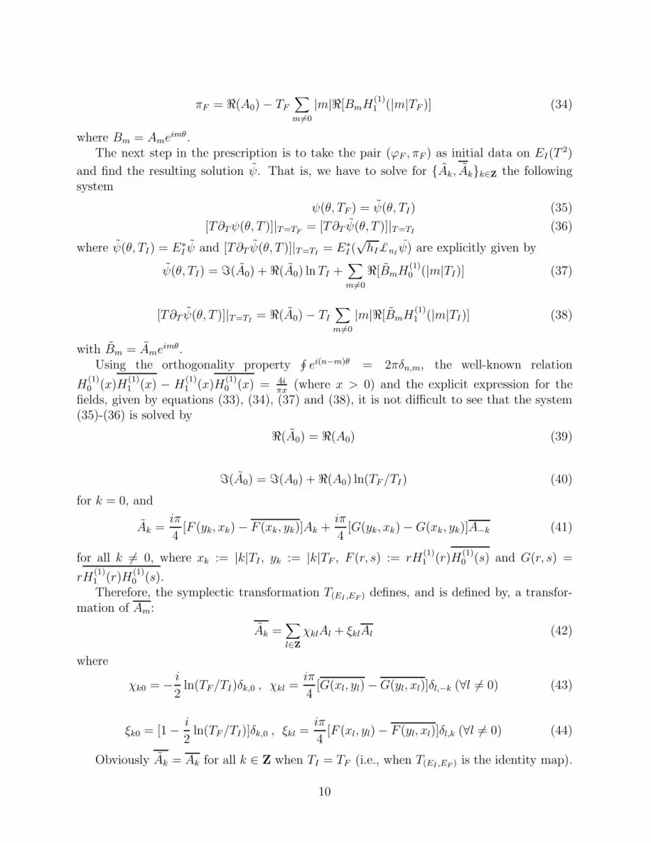
πF = ℜ(A0) − TF∑

m6=0

|m|ℜ[BmH(1)1 (|m|TF )] (34)

where Bm = Ameimθ.

The next step in the prescription is to take the pair (ϕF , πF ) as initial data on EI(T2)

and find the resulting solution ψ. That is, we have to solve for Ak, Akk∈Z the followingsystem

ψ(θ, TF ) = ψ(θ, TI) (35)

[T∂Tψ(θ, T )]|T=TF = [T∂T ψ(θ, T )]|T=TI (36)

where ψ(θ, TI) = E∗I ψ and [T∂T ψ(θ, T )]|T=TI = E∗

I (√hI£nI

ψ) are explicitly given by

ψ(θ, TI) = ℑ(A0) + ℜ(A0) lnTI +∑

m6=0

ℜ[BmH(1)0 (|m|TI)] (37)

[T∂T ψ(θ, T )]|T=TI = ℜ(A0) − TI∑

m6=0

|m|ℜ[BmH(1)1 (|m|TI)] (38)

with Bm = Ameimθ.

Using the orthogonality property∮

ei(n−m)θ = 2πδn,m, the well-known relation

H(1)0 (x)H

(1)1 (x) − H

(1)1 (x)H

(1)0 (x) = 4i

πx(where x > 0) and the explicit expression for the

fields, given by equations (33), (34), (37) and (38), it is not difficult to see that the system(35)-(36) is solved by

ℜ(A0) = ℜ(A0) (39)

ℑ(A0) = ℑ(A0) + ℜ(A0) ln(TF/TI) (40)

for k = 0, and

Ak =iπ

4[F (yk, xk) − F (xk, yk)]Ak +

iπ

4[G(yk, xk) −G(xk, yk)]A−k (41)

for all k 6= 0, where xk := |k|TI , yk := |k|TF , F (r, s) := rH(1)1 (r)H

(1)0 (s) and G(r, s) =

rH(1)1 (r)H

(1)0 (s).

Therefore, the symplectic transformation T(EI ,EF ) defines, and is defined by, a transfor-mation of Am:

Ak =∑

l∈Z

χklAl + ξklAl (42)

where

χk0 = − i

2ln(TF/TI)δk,0 , χkl =

iπ

4[G(xl, yl) −G(yl, xl)]δl,−k (∀l 6= 0) (43)

ξk0 = [1 − i

2ln(TF/TI)]δk,0 , ξkl =

iπ

4[F (xl, yl) − F (yl, xl)]δl,k (∀l 6= 0) (44)

Obviously Ak = Ak for all k ∈ Z when TI = TF (i.e., when T(EI ,EF ) is the identity map).

10

B. Quantum Implementability

The question we want to address in this part is whether or not classical evolution onthe fictitious background is implementable at the quantum level. A particularly convenientapproach to this issue is given by the algebraic approach of QFT, since the notion of im-plementability of symplectic transformations on a Hilbert space formulation is defined ina natural way [14]. The main idea in the algebraic approach is to formulate the quantumtheory in such a way that the observables become the relevant objects and the quantumstates are “secondary”, they are taken to “act” on operators to produce numbers. The basicingredients of this formulation are two, namely : (1) a C∗-algebra A of observables, and (2)states ω : A → C, which are positive linear functionals (ω(A∗A) ≥ 0 ∀A ∈ A) such thatω(1) = 1. The value of the state ω acting on the observable A can be interpreted as theexpectation value of the operator A on the state ω, i.e., 〈A〉 = ω(A).

For free (linear) fields it is possible to construct the Weyl algebra of quantum abstractoperators from the elementary classical observables (equipped with an algebraic structuregiven by the Poisson bracket). The elements of this C∗-algebra are taken to be the funda-mental observables for the quantum theory, thus the (natural) algebra A for free fields is theWeyl algebra. Let (Y,ΩY ) be a symplectic vector space, each generator W (y) of the Weylalgebra is the “exponentiated” version of the linear observable ΩY (y, · ). These generatorssatisfy the Weyl relations1:

W (y)∗ = W (−y) , W (y1)W (y2) = e−i2ΩY (y1,y2)W (y1 + y2) (45)

Given a symplectic transformation f on Y , there is an associated ∗-automorphism of A,αf : A → A, defined by αf ·W (y) := W (f [y]). In particular, the symplectic transformationT(EI ,EF ) representing time evolution from EI = (TI , x

i) to EF = (TF , xi) defines the ∗-

automorphism α(EI ,EF ). Thus, from the algebraic point of view, if we assign the state ω tothe initial time as represented by the embedding EI , the expectation value of the observableW ∈ A on EI is given by

〈W 〉EI = ω(W ) (46)

Let us consider the Weyl generator W (ψ) labeled by ψ. Under the symplectic transforma-tion T(EI ,EF ), the label goes to ψ and the relation between W (ψ) and W (ψ) is given by

α(EI ,EF )W (ψ) = W (ψ). Since T(EI ,EF ) dictates time evolution at classical level, one caninterpret the change W (ψ) → α(EI ,EF )W (ψ) as a counterpart in the observables. That is,W (ψ) → α(EI ,EF )W (ψ) is the mathematical representation of time evolution of observablesin the Heisenberg picture. Thus, while in the Heisenberg picture the expectation value of theobservable W (ψ) at final time is given by 〈W (ψ)〉EF = ω(α(EI ,EF ) ·W (ψ)), in the Schrodingerpicture is 〈W (ψ)〉EF = ωEF (W (ψ)). Therefore, the final state ωEF , obtained by evolving theinitial state ω, is given by ω α(EI ,EF ).

Now, in order to know if time evolution between any two flat Cauchy surfaces is welldefined in the framework of the Hilbert space formulation, we have to introduce the GNS

1The CCR that correspond to operators ΩY (y, · ) get now replaced by the quantum Weyl relations.

11

construction that tells us how the quantization in the old sense (that is, a representation ofthe Weyl relations on a Hilbert space) and the algebraic approach are related:

Let A be a C∗-algebra with unit and let ω : A → C be a state. Then there exista Hilbert space H, a representation π : A → L(H) and a vector |Ψ0〉 ∈ H such that,ω(A) = 〈Ψ0, π(A)Ψ0〉H. Furthermore, the vector |Ψ0〉 is cyclic. The triplet (H, π, |Ψ0〉) withthese properties is unique (up to unitary equivalence).

With this in hand, we have a precise way to ‘go down’ transformations on the C∗-algebrato a given Hilbert space representation. Thus, a symplectic transformation f : Y → Y , withcorresponding algebra automorphism αf : A → A, is unitarily implementable [14] if thereis a unitary transformation U : H → H on the Hilbert space H such that, for any W ∈ A,U−1π(W )U = π(αf ·W ).

Because ω and its transform ω αf will not always define unitarily equivalent Hilbertspace representations, thus not all symplectic transformations f will be implementable infield theory. In our case, we are interested on the implementability of f = T(EI ,EF ) on thesymmetric Fock space F , constructed from the so-called “one-particle” Hilbert space, H0,which elements are the complex functions

Ψ =∑

m∈Z

fm(θ, T )Am (47)

determined by the natural splitting of VC, the complexification of V , on negative and positiveparts through the complex structure JV .

The continuous2 transformation (42) defines a pair of bounded linear maps ξ : H0 → H0

and χ : H0 → H0, where H0 is the complex conjugate space to H0. With Ψ given by (47),we have

ξ · Ψ =∑

m,l∈Z

fm(θ, T )ξml Al (48)

and

χ · Ψ =∑

m,l∈Z

fm(θ, T )χml Al (49)

The automorphism α(EI ,EF ) associated with T(EI ,EF ) is unitarily implementable with respectto the Fock representation (F = Fs(H0), π) if and only if the operator χ is Hilbert-Schmidt[17]. i.e., iff

∑

m,l∈Z

|χlm|2 <∞ (50)

Since∑

m,l∈Z |χlm|2 = |12ln(TF/TI)|2 +

∑

l,m6=0 |χlm|2, then according to Eq.(43) condition(50) is equivalent to

∑

m6=0

(ℜ[gm(xm, ym)])2 <∞ and∑

m6=0

(ℑ[gm(xm, ym)])2 <∞ (51)

2Actually, it can be shown that there is a constant b such that, for all ψ ∈ V , ||T(EI ,EF )ψ|| ≤ b||ψ||in the norm ||ψ||2 = ΩV (JV ψ,ψ).

12

where gm(r, s) := G(r, s)−G(s, r). Using the definition of Hankel function in terms of Besseland Neumann functions (for n = 0 or 1), the first condition in (51) can be written as follows

∞∑

m=1

(Λm[a, ym])2 <∞ (52)

where Λm[a, ym] := m[a(J0(ym)J1(aym) − N0(ym)N1(aym)) + N1(ym)N0(aym) −J1(ym)J0(aym)] and a := TI/TF . In the asymptotic region x ≫ 1 (for n = 0 or 1) the

behavior of Bessel and Neumann functions is given by Jn(x) ≈√

2πx

cos(x − (n + 12)π

2) and

Nn(x) ≈√

2πx

sin(x−(n+ 12)π

2) respectively, then Λm[a, ym] ≈ 2m√

aπym(a−1) cos(ym(1+a)−π)

for m≫ 1 is the asymptotic behavior of Λm[a, ym] and (52) becomes

4(1 − a)2

aπ2T 2F

∞∑

m=N

cos2(TF (1 + a)m) <∞ (53)

where N ≫ 1. Notice that for the case a = 1 this condition is trivially satisfied, as expected.Thus, unitary implementability implies that (53) is satisfied for all a ∈ (0, 1) and

hence, if there are particular values of TF (r0 > 0) and a (a0 ∈ (0, 1)) such that∑∞m=N cos2(r0(1 + a0)m) diverges, then α(EI ,EF ) will not be unitarily implemented. In

particular, by choosing TF = π1+a

every integer m ≥ N corresponds to a maximum ofcos2(TF (1 + a)x) and therefore the sum in (53) diverges. Thus, the transformation associ-ated with T(EI ,EF ) is not unitarily implementable with respect to the Fock representation(Fs(H0), π) and hence classical time evolution, dictated by T(EI ,EF ), does not have a quantumanalog in the Hilbert space formulation via a unitary operator. In this case, the Schrodingerpicture is not available to describe functional evolution using the Fock space representa-tion of the quantum theory, consequently the “Schrodinger equation” associated with theHamilton operator H(T ) can not be interpreted as an evolution equation (on the fictitiousbackground) for quantum states.

IV. DISCUSSION AND CONCLUSIONS

In this work we have analyzed the quantization of polarized Gowdy T 3 cosmologicalmodels as carried out by Pierri. We have found explicitly the symplectic transformation thatdetermines the classical dynamical evolution T(EI ,EF ) given by the phase space function T .We have shown that this symplectic transformation does not have a quantum analog in theHilbert space formulation via a unitary operator. This means that the classical dynamics ofGowdy T 3 cosmological models cannot be implemented in the context of Pierri’s quantizationprocedure. Let us now discuss the implications of this negative result for two related areas,namely for canonical quantum gravity and for quantization of fields on curved manifolds.

Canonical Quantum Gravity.First of all let us recall that in canonical quantum gravity, the theory is defined over

an “abstract” manifold Σ which in our case is given by Σ = T 2. There is no spacetimeand therefore no notion of an embedding of Σ into this spacetime. What we have is, in thegauge fixed scenario, a reduced phase space representing the true degrees of freedom, and,

13

in the quantum theory, a Hilbert space of physical states and physical observables definedon it. This is the frozen formalism description. When the deparametrization procedurewas introduced classically, an artificial notion of time evolution was created that allows to“evolve” any set of (physical) initial conditions on Σ into a one parameter family of initialconditions with a precise spacetime interpretation. This one parameter family is generatedvia a canonical transformation generated by the reduced Hamiltonian. In quantum gravity,however, the parameter T can not be thought, a priory, as a a time function in a spacetimefor the only reason that a spacetime notion is absent. In which sense is then useful theparameter T ? Recall from the discussion in Sec. III that the notion of time evolution inthe algebraic formulation is well defined, giving rise to the Heisenberg picture: We have aunique state |Ψ〉T0, defined on a preferred and fixed Σ0, and operators acting on it whichcould be “time dependent”. This is the place where the parameter T plays a central role.We can have, for instance, a one parameter family of observables, say VT , corresponding to“the volume of the Universe at time T” [5]. In the standard formulation of quantum theory,where a unitary evolution operator U(T, T0) exists, we can relate the operators belongingto the family via unitary transformations. One can also construct the Schrodinger pictureand have a one-parameter family of states that “evolve” in time T , using the standardconstruction. Canonical quantum gravity is most naturally constructed in the Heisenbergpicture, where the physical operators correspond to the so called “evolving constants ofthe motion”. Therefore, any operator OT labeled by the time T , if it is well defined (i.e.if it leaves the Hilbert space, or a dense subset of it, invariant), can be regarded as aphysically meaningful object representing the classical observable at “time T”. What is lostin the absence of the operator U(T, T0), as is our case, is the “unitary equivalence” of theoperators OT for all values of T . In this sense, unitary time evolution and the Schrodingerpicture are lost. Unitary evolution is one of the pillars of present quantum theory, andtheories that do not satisfy this property suffer from the rejection of the community, sincethe theory becomes unable to make predictions due to the lack of conservation of probability.This would be the case, for instance, in the event of the evaporation of a black hole viaHawking radiation. Physicists have always tried to avoid such descriptions and look forexplanations that are “unitary”. However, as we would like to argue, canonical quantumgravity is conceptually very different from the standard description of quantum theory witha preferred and external Newtonian time, so one should look for more involved argumentsbefore dismissing a particular theory. In the Hamiltonian description, time evolution is puregauge, so strictly speaking one should only meaningfully discuss physical observables on thereduced phase space. There is no time evolution and no dynamics. Any deparametrization isclassically equivalent, giving rise to fictitious dynamics via canonical transformations. Thereis no compelling reason to expect that there is a preferred deparametrization that will bemeaningful quantum-mechanically. Thus, there is no logical contradiction to the result thata particular choice can not be unitarily implemented.

Within this perspective, the parameter T that was introduced artificially at the classicallevel bears no fundamental physical significance. The fact that the quantum theory doesnot endorse this choice should not be enough reason to dismiss it. However, it should beclear that the absence of unitary transformation reduces significantly the importance ofthis quantization, since the Heisenberg operators OT are not well defined. That is, theirspectra, expectation values, etc., depend on the choice of the value of T0. Had we chosen a

14

different value T = T ′0 and therefore different Heisenberg state |Ψ〉T ′

0, we would get different

operators O′T 6= OT (for the same value of T ). A minimum requirement for the consistency

of the quantization is that the operators O′T and OT be (unitary) equivalent. Thus, the

quantization is physically unacceptable.However, it is not completely clear whether this negative result holds for any choice of a

set of creation and annihilation operators (or, equivalently, choice of complex structure J).The original choice in Ref. [4] seems natural from the viewpoint of the explicit form of thesolutions of the Klein-Gordon equation, and the fact that is time independent and thereforethere is no “particle creation”. However, further work is needed in order to understandwhether there exist different choices of J and therefore of representations of the CCR forwhich “time evolution” is a well defined concept. Unitary implementability might even bea criteria leading to a physically relevant quantization.

Quantum Fields on Curved Surfaces.The issue of formulating time evolution between arbitrary Cauchy surfaces in the quan-

tum theory of fields goes back to the work of Dirac [18]. However, it is only recently thatunitary implementability of arbitrary time evolution has been considered. Somewhat surpris-ingly, it has been recognized that even for free fields on Minkowski spacetime, time evolutionbetween arbitrary Cauchy surfaces is not unitarily implementable in three and higher space-time dimensions [14]. The failure is in general attributed to the fact that time evolutionbetween arbitrary surfaces is not generated by an isometry of the background metric [12,14].It is also known that in two dimensions, for the standard quantization coming from thesymmetries of the system, time evolution is well defined for arbitrary Cauchy surfaces withtopology of a circle. However, for our model, even when it is a truly two dimensional model(ψ depends only on θ and T ), it does not satisfy a free scalar equation (it is instead relatedto a Liouville model). Therefore, there is no contradiction with the fact that time evolutionis not unitary. From the three dimensional perspective, the theory is given by a free scalarfield on a flat background, but in which the vector field ∂/∂T that generates the naturaltime evolution is not an isometry of the background spacetime. Thus, it is interesting to seethat in this case, even for the simplest Cauchy surfaces (flat and parallel in the given chart),time evolution is not implementable. It is also interesting to note that particle creationand non-unitary time evolution do not imply each other, as noted in [14]. As previouslymentioned, it is not clear whether different representations of the CCR would yield unitaryquantum theories. Namely, is there a choice of J that will render the theory unitary? Wouldit be unique? We shall leave these questions for future investigations.

Note added: After submitting this paper, we learned that similar results were independentlyfound by Torre [20].

ACKNOWLEDGMENTS

We would like to thank the referee for helpful comments and C. Torre for correspondence.This work has been supported by DGAPA–UNAM grant No. IN-112401 and CONACYTgrants 36581-E and J32754-E. This work was also partially supported by NSF grant No.PHY-0010061. J.C. was supported by a CONACYT-UNAM(DGEP) Graduate Fellowship.

15

REFERENCES

[1] C. W. Misner, In Magic without Magic: John Archibald Wheeler, J. Klauder (Ed.)(Freeman, San Francisco, 1972).

[2] C. G. Torre, “Midisuperspace models of canonical quantum gravity,” Int. J. Theor.Phys. 38, 1081 (1999).

[3] A. Ashtekar and M. Pierri, “Probing quantum gravity through exactly soluble midi-superspaces. I,” J. Math. Phys. 37, 6250 (1996).

[4] M. Pierri, “Probing quantum general relativity through exactly soluble midi-superspaces. II: Polarized Gowdy models,” Int. J. Mod. Phys. D 11, 135 (2002).

[5] M. Pierri, “Hamiltonian and volume operators,” arXiv:gr-qc/0201013.[6] R. H. Gowdy, “Gravitational Waves In Closed Universes,” Phys. Rev. Lett. 27, 826

(1971); Ann. Phys. 83, 203 (1974).[7] B. K. Berger, Ann. Phys. 83, 458 (1974); “Quantum Cosmology: Exact Solution For

The Gowdy T 3 Model,” Phys. Rev. D 11, 2770 (1975).[8] C. W. Misner, “A minisuperspace example: The Gowdy T 3 cosmology”, Phys. Rev.

D8, 3271 (1973).[9] V. Husain, “Quantum Effects on the syngularity of the Gowdy Cosmology”, Class.

Quantum Grav. 5, 1587 (1987).[10] G. A. Mena Marugan, “Canonical quantization of the Gowdy model,” Phys. Rev. D 56,

908 (1997).[11] K. Kuchar, “Dirac Constraint Quantization of a Parametrized Field Theory by Anomaly

- Free Operator Representations of Space-Time Diffeomorphisms,” Phys. Rev. D 39,2263 (1989); K. Kuchar, “Parametrized Scalar Field on R × S(1): Dynamical Pic-tures, Space-Time Diffeomorphisms, and Conformal Isometries,” Phys. Rev. D 39, 1579(1989).

[12] A. D. Helfer, “The Stress-Energy Operator,” Class. Quant. Grav. 13, L129 (1996)[arXiv:gr-qc/9602060].

[13] C. G. Torre and M. Varadarajan, “Quantum fields at any time,” Phys. Rev. D 58,064007 (1998).

[14] C. G. Torre and M. Varadarajan, “Functional evolution of free quantum fields,” Class.Quant. Grav. 16, 2651 (1999).

[15] N. D. Birrel and P. C. W. Davies, Quantum fields in curved space (Cambridge UniversityPress, Cambridge, 1982).

[16] A.Ashtekar, L.Bombelli and O.Reula, in Mechanics, Analysis and Geometry: 200 YearsAfter Lagrange (North-Holland, New York 1991); R.M.Wald, Quantum Field Theoryin Curved Spacetime and Black Hole Thermodynamics (University of Chicago Press,Chicago, 1994).

[17] R.Honegger and A.Rieckers, “Squeezing Bogoliubov transformations on the infinitemode CCR-algebra”, J. Math. Phys. 37, 4291 (1996).

[18] P.A.M. Dirac, Lectures on Quantum Mechanics, (New York, Yeshiva University, 1964).[19] G.B. Arfken and H.J. Weber, Mathematical Methods for Physicists, (Academic Press,

1995).[20] C. G. Torre, private communication.

16