arX

iv:1

012.

5293

v1 [

quan

t-ph

] 2

3 D

ec 2

010

Phase Estimation with Non-Unitary Interferometers: Information as a Metric

Thomas B. BahderAviation and Missile Research, Development, and Engineering Center,

US Army RDECOM, Redstone Arsenal, AL 35898, U.S.A.(Dated: December 24, 2010)

Determining the phase in one arm of a quantum interferometer is discussed taking into account thethree non-ideal aspects in real experiments: non-deterministic state preparation, non-unitary stateevolution due to losses during state propagation, and imperfect state detection. A general expressionis written for the probability of a measurement outcome taking into account these three non-idealaspects. As an example of applying the formalism, the classical Fisher information and fidelity(Shannon mutual information between phase and measurements) are computed for few-photon Fockand N00N states input into a lossy Mach-Zehnder interferometer. These three non-ideal aspects leadto qualitative differences in phase estimation, such as a decrease in fidelity and Fisher informationthat depends on the true value of the phase.

I. INTRODUCTION

Optical interferometers [1] and matter wave inter-ferometers [2] have been of great interest because oftheir practical applications in metrology. Interferome-ters have been used to measure such diverse quantitiesas electric, magnetic, and gravitational fields, gravita-tional waves [2–4], and there are plans to use them totest the theory of general relativity [5]. Classical opticalinterferometers [6] have been routinely used for sensingrotation in gyroscopic applications based on the Sagnaceffect [7–11] and experiments with Sagnac interferome-ters have been done with single-photons [12], with Bose-Einstein condensates(BEC) [13–15], and schemes usingentangled particles have been proposed that are capableof Heisenberg limited precision measurements that scaleas 1/N , where N is the number of particles [16].On a more fundamental level, there is interest in inter-

ferometers because they are a vehicle to study the limitsof precision of quantum measurements [17–19]. Perhapsthe simplest generic measurement problem consists of de-termining the relative phase shift between two arms of aninterferometer from measurements made at the outputports of the interferometer [20–25]. This phase shift maybe related to a classical external field incident on a phaseshifter in one arm of the interferometer, in which case theinterferometer can be used as a sensor of the field [26].The determination of the phase shift is a specific exam-ple of the more general problem of parameter estimation,whose goal is to determine one or more parameters frommeasurements [27–34].Recently, there have been experimental demonstra-

tions using entangled states to estimate the phase shiftin one arm of a Mach-Zehnder interferometer [21, 35–37].Even more recently, the effect of losses on phase deter-mination was studied experimentally [38]. In real ex-periments, there are three non-ideal elements of the in-terferometer system: state preparation [36, 39], photonlosses in the interferometer [38] and non-ideal photon-number detection [21, 37]. Phase estimation has beentheoretically investigated by separately taking into ac-count non-deterministic state preparation [28–34], pho-

ton losses in the interferometer itself [24, 25, 40–45] andphoton-number counting efficiency [25, 37, 46].

In this work, I write down a formalism that simulta-neously takes into account, in a unified way, all three ofthe non-ideal elements in experiments: non-deterministicstate preparation, propagation through a lossy interfer-ometer, and imperfect state detection. Non-deterministicstate preparation must be described by a density matrix,rather than by a pure state, thereby allowing for the finiteprobability of creating states other than intended. Whenthe optical state is created, it enters the interferometer,where propagation may be non-ideal because photon ab-sorption and scattering can occur. Finally, when the opti-cal state leaves the interferometer, it enters the detectionsystem, which may also be non-ideal: the state registeredby the detection system may not be the true state thatentered the detection system.

Much of the previous work was focused on determin-ing the optimum measurements for determining phaseand hence the quantum Fisher information was of pri-mary interest, because it gives a bound on the vari-ance of the phase associated with the optimum measure-ment [28–33, 46–49]. In contrast, in this work I lookat the information gain from specific, simple, photon-number counting measurements that can be easily imple-mented in the laboratory, and hence the classical Fisherinformation is the quantity of interest because it dependson the particular measurement that is performed.

In Section II, I briefly review the theory of phase de-termination based on parameter estimation (Fisher in-formation) and on fidelity (Shannon mutual informationbetween measurements and phase). In Section III, I in-troduce an example of a non-ideal interferometer system,where state evolution is non-unitary. I write a statisticalexpression for the probability of measurement outcomesthat takes into account the three non-ideal componentsof the interferometer system described above. I use thisprobability in the classical Fisher information in Eq. (2)and in the fidelity in Eq. (9) to analyze the determinationof phase in a non-ideal interferometer system. As simpleexamples of the formalism, in sub-sections of Section III,I look at few photon examples of non-deterministic state

2

preparation, propagation through a non-unitary (lossy)interferometer, and imperfect state detection. Finally, inSection IV, I make some concluding remarks. My goalis to look at examples of few-photon states that can beimplemented experimentally, with the hope that the ex-amples and method described here can be helpful for an-alyzing real experiments. Furthermore, in this work, Irestrict myself to the simple case of non-adaptive mea-surements [50], where the measurement is fixed beforephase estimation.

II. THEORETICAL BACKGROUND

The accuracy of estimating a (single) one-dimensionalparameter, φ, is described in terms of the classicalCramer-Rao bound [51], which gives a lower bound onthe variance (δφ)2 of an unbiased estimator of the pa-rameter φ:

(δφ)2 ≥ 1

Fcl(φ;M)(1)

where Fcl(φ;M) is the classical Fisher information givenby [27, 51]

Fcl(φ;M) =∑

ξ

1

P (ξ|φ, ρ)

[

∂P (ξ|φ, ρ)∂φ

]2

(2)

The classical Fisher information is described in termsof the conditional probability distribution, P (ξ|φ, ρ), formeasurement outcome, ξ, which can take one or morecontinuous values, or, one or more discreet values. If ξtakes continuous values, the sum over ξ in Eq. (2) is anintegral. For the case of quantum measurements, theseprobabilities are given by

P (ξ|φ, ρ) = tr(

ρφ Πo (ξ))

= tr(

ρo Πφ (ξ))

(3)

where the state is specified by the Schrodinger pic-ture density matrix, ρφ, and the measurements bythe positive-operator valued measure (POVM) in the

Schrodinger picture, Πo(ξ). The POVM are set a of non-

negative Hermitian operators, M = {Π(ξ)}, represent-ing a given physical measurement and so the expectationvalue of each operator Πo(ξ) is non-negative, and satisfies∑

ξ

Πo(ξ) = I, where I is the identity operator. Alterna-

tively, in the Heisenberg picture, the state is given by thedensity matrix, ρo, and probabilities of measurements byPOVM, Πφ(ξ). Operators in the Schrodinger and Heisen-

berg pictures, OS and OH(φ), respectively are related by

OH(φ) = U †(φ) OS U(φ), and U(φ) = exp(−iφh), whereh is the infinitesimal displacement operator for the pa-rameter φ, satisfying

i∂

∂φ|ψ(φ)〉 = h |ψ(φ)〉 (4)

The quantum Fisher information, FQ(φ) is obtained bymaximizing the classical Fisher information, Fcl(φ;M),over all possible measurements M , at a given value ofφ. Braunstein and Caves [31, 32] have shown that an

improved lower bound is possible for the variance, (δφ)2,

in terms of the quantum Fisher information:

(δφ)2 ≥ 1

Fcl(φ;M)≥ 1

FQ(φ)(5)

where FQ(φ) is independent of the measurementM . Thequantum Fisher information is defined by

FQ (φ) = tr[

ρφΛ2φ

]

(6)

where the Hermitian operator, Λφ, is the symmetric log-arithmic derivative (S.L.D.), defined implicitly by

∂ρφ∂φ

=1

2

[

Λφ ρφ + ρφΛφ

]

(7)

The right side and left side of the inequality in Eq. (5)is sometimes called the quantum Cramer-Rao bound, seealso the work by Helstrom [28, 29] and Holevo [30], anddiscussion by Barndorff-Nielsen et al. [33, 34]. The ex-pression in Eq. (5) provides a bound on the variance of anunbiased estimator for an optimum measurement. How-ever, the theory does not give a procedure for determin-ing the optimum measurement. For one-dimensional pa-rameter estimation and for simple (non-adaptive) mea-surements, Barndorff-Nielsen and Gill have shown that ingeneral the optimum measurementM will depend on theparameter φ, which is unknown prior to estimation [33].Consequently, Barndorff-Nielsen and Gill have proposeda two-stage adaptive measurement procedure that willgive

Fcl(φ;M) = FQ (φ) (8)

for optimum measurement M for all φ.For the case of a pure state, |ψo〉, where the density

matrix is ρo = |ψo〉 〈ψo|, and where the path is generated

by a unitary transformation, U(φ), the quantum Fisherinformation, FQ(φ), does not depend on φ [32, 48, 49],

and is given by the fluctuations of the generator h byFQ (φ) = 4(∆h)2. Hofmann has shown [52] that forpure states (which are most states considered in ideal-ized non-classical phase measurements) a path-symmetryis responsible for the quantum Fisher information beingindependent of φ.In Section III below, I consider the case of a lossy

Mach-Zehnder interferometer, where the state evolutionis effectively non-unitary, thereby leading to a classicalFisher information that depends on the true value of thephase φ.The above discussion of parameter estimation is based

on classical and quantum Fisher informations, which arelocal descriptions of phase estimation, because they de-pend on the true value of φ. Complementary to the above

3

local descriptions, is a global description given by the fi-delity [26]:

H(M) =∑

ξ

∫ +π

−π

dφ P (ξ|φ, ρ) p(φ) ×

log2

[

P (ξ|φ, ρ)∫ +π

−πP (ξ|φ′, ρ) p(φ′) dφ′

]

. (9)

where P (ξ|φ, ρ) is given in Eq. (3). The fidelity, H(M),is the Shannon mutual information [51, 53] between themeasurement M and the unknown parameter φ. The fi-delity, H(M), gives the average amount of information(in bits) about the parameter φ that can be obtainedfrom the measurement M for one use (one measurementcycle) of the interferometer. The fidelity does not dependon φ because it is an average over all possible phases φand over all probabilities of measurement outcomes for agiven POVM M . (For an alternative discussion of localversus global phase estimation, see Ref.[22].) The fidelityalso depends on the prior information about the param-eter φ through the prior probability distribution p(φ).Consequently, the fidelity characterizes the quality of theinterferometer system as a whole, in terms of mutual in-formation between the measurement M and the param-eter φ. Note that the fidelity depends on the input statedensity matrix, ρ, and the measurement M , and there-fore can be used to optimize the system with respect tothe input state and measurement. The fidelity is a mea-sure of the information that flows from the phase φ tothe measurements, which is analogous to a communica-tion problem where Alice sends messages to Bob. In thecase of the measurement problem, quantum fluctuationsin the initial state, in the channel (interferometer), andthe type of measurement, determine the amount of infor-mation that is obtained about the parameter φ from themeasurements. The fidelity has been applied to comparethe use of Fock states and N00N states when no prior in-formation is present about the phase [26] and when thereis significant prior information about the phase [54].The complimentary measures of fidelity and Fisher in-

formation may be contrasted as follows. Assume that Iwant to shop to purchase the best measurement deviceto determine the unknown parameter φ. If I do not knowthe true value of the parameter φ, I would compare theoverall performance specifications of several devices andI would purchase the device with the best over-all spec-ifications for measuring φ. The fidelity, H(M), is theover-all specification for the quality of the device, so Iwould purchase the device with the largest fidelity. AfterI have purchased the device, I want to use it to deter-mine a specific value of the parameter φ based on severalmeasurements (data). This involves parameter estima-tion, which requires the use of Fisher information, anddepends on the true value of the parameter φ.Historically, the variance, (δφ)2, of the estimated pa-

rameter φ has been discussed in terms of the stan-dard quantum limit, δφSL = 1/

√N , and the Heisenberg

Quantum

state preparation DetectionOptical

Interferometer

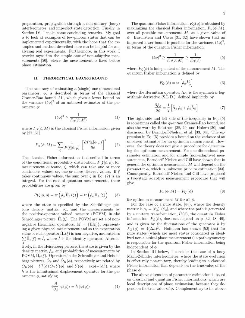
PSIΨkinM PIIΨ j

out Ψkin, ΦM PDIΞ Ψ j

out, ΦM

FIG. 1. Interferometer system shown with three components:state preparation, interferometer, and detection system.

limit[4, 18, 55, 56], δφHL = 1/N , where N is the num-ber of particles or quanta that enter the interferometerduring each measurement cycle. The value δφ is presum-ably the width of some probability distribution, p(φ|ξ, ρ),such as the distribution calculated from Bayes’ rule, seeEq. (25). Detailed calculation of p(φ|ξ, ρ) for a number ofinput states shows that these distributions have multiplepeaks [26]. Consequently, rather than using the widthsof these distributions as a metric for determining φ, Iuse the information measures, Fisher information and fi-delity, which naturally handle distributions with multiplepeaks.

III. NON-IDEAL OPTICAL SYSTEM

As described in the introduction, an interferometer sys-tem can be divided into three parts: state creation, stateevolution through the optical interferometer, and detec-tion of the output state. In a real experiment, each ofthese three parts can be non-ideal, see Fig. 1. For exam-ple, I may want to create a quantum state |ψin〉 as inputinto the interferometer. However, instead, the resultingstate may be a mixture of states, each with some prob-ability, PS(ψ

ink ), for k = 1, 2, · · · . Such a quantum state

is described by the density matrix ρ:

ρ =∑

k

PS(ψink )

∣

∣ψink

⟩ ⟨

ψink

∣

∣ (10)

The state ρ is then input into the interferometer, wherethere may be absorption and scattering of photons. Forexample, a two-photon state may enter the interferometerand a one-photon state may exit the interferometer, be-cause one photon was absorbed inside the interferometer.Alternatively, a two-photon state may enter the interfer-ometer and a three-photon state may exit the interferom-eter, due to light scattering into the interferometer fromthe environment. I can describe these processes gener-ally by a transfer matrix, PI(ψ

outj |ψin

k , φ), which gives

the conditional probability for state∣

∣ψoutj

⟩

to exit the

interferometer given that state∣

∣ψink

⟩

entered the interfer-

ometer. The transfer matrix, PI(ψoutj |ψin

k , φ), is generalenough to describe non-unitary propagation of the quan-tum state through the interferometer, and so can take

4

into account losses and scattering. Note that the trans-fer matrix may depend on the state of the interferome-ter, which I specify here by single parameter φ. Finally,the detection of the quantum state that leaves the inter-ferometer can be non-ideal. For example, the detectionsystem may register a measurement ξ, when state |ψout

i 〉enters the detection system, whereas the true state thatentered the detection system was

∣

∣ψoutj

⟩

. I can representsuch an imperfect detection system by the conditionalprobability PD(ξ|ψout

j , φ), which gives the probability for

making a measurement ξ when state ψoutj entered the

detection system. Note that in general this probabilitymay or may not depend on φ, a parameter describing thestate of the interferometer. For a non-ideal interferome-ter system, the probability of obtaining a measurementξ is given by [57]

P (ξ|φ) =∑

j

PD(ξ|ψoutj , φ)

∑

k

PI(ψoutj |ψin

k , φ) PS(ψink )

(11)

where we must have each of the three probabilities sumto unity:

∑

k

PS(ψink ) = 1 (12)

∑

j

PI(ψoutj |ψin

k , φ) = 1 (13)

∑

ξ

PD(ξ|ψoutj , φ) = 1 (14)

Equation (11) is a general statistical relation for theprobability of obtaining a measurement outcome ξ forgiven phase shift φ, taking into account the three non-ideal aspects of interferometer systems. Note thatEq. (11) is sufficiently general that it can be applied tothe case where states are represented by density matrices.In this case, in Eq. (11) we can make the replacementsψink → ρink and ψout

j → ρoutj , where ρink and ρoutj are aset of input and output density matrices labeled by inte-gers j, k = 1, 2, · · · . In order to compute the probabilitiesof measurement outcomes, P (ξ|φ), Eq. (11) must be aug-mented by a detailed model of input and output states. Igive several examples of applying Eq. (11) in the sectionsthat follow.The probability of measurement outcome, given by

Eq. (11), enters into the Fisher information and into theShannon mutual information, in Eq. (2) and Eq. (9), re-spectively. In the next three subsections, A, B, and C,I give examples of the effects of non-deterministic statepreparation, state evolution through an interferometerwhen absorption is present, and imperfect output statedetection, respectively, using Fisher and Shannon mutualinformations as metrics of performance of the interferom-eter.

A. Non-Deterministic State Preparation

Consider an optical interferometer system that hasnon-deterministic state preparation, but has no lossesin the interferometer and has perfect state detection.When I try to prepare a certain quantum state for in-put into the interferometer, there is always a non-zeroprobability that another state than intended will be pre-pared. This non-deterministic state preparation is ex-pressed by a density matrix for the input state, whichassigns probabilities for creating various quantum states,see Eq. (10). Since state detection is assumed perfect,PD(ξ|ψout, φ) = 1 when the measurement ξ correspondsto the true state that entered the detection system, ψout,and otherwise PD(ξ|ψout, φ) = 0.A general interferometer with no losses is characterized

by a unitary scattering matrix, Sij(φ), that connects theNp input-mode field operators, αi, to the Np output field

operators, βi:

βi =

Np∑

j=1

Sij(φ) αj = U †(φ)αiU(φ) (15)

where U(φ) is a unitary evolution operator, i, j =1, 2, · · · , Np, and φ is one or more parameters (e.g., phaseshift) that describe the state of the interferometer.For simplicity, I consider a Mach-Zehnder interferom-

eter, with no losses, with input ports labeled, “a” and“b”, and output ports, “c” and “d”, having a scatteringmatrix

Sij(φ) =1

2

(

−i(

1 + eiφ) (

−1 + eiφ)

(

−1 + eiφ)

i(

1 + eiφ)

)

(16)

where αi = {a, b} and βi = {c, d}.The probabilities, PI(ψ

outj |ψin

k , φ), that relate the in-

put state ψink to the output state ψout

j of the interfer-ometer are given in terms of the projection operatorsΠφ (nc, nd):

PI(ψoutj |ψin

k , φ) =⟨

ψink

∣

∣ Πφ (nc, nd)∣

∣ψink

⟩

(17)

where the output state ψoutj is specified by two inte-

gers, {nc, nd}, giving the photon numbers output in ports“c” and “d”. In terms of the unitary evolution opera-tor, U(φ), the output state in the Schrodinger picture is

|ψout(φ)〉 = U(φ)∣

∣ψin⟩

, where∣

∣ψin⟩

is the Heisenbergpicture input state. In Eq. (11), the sum over k is nowa double sum over all non-negative values of the two in-tegers nc and nd. For a generic Mach-Zehnder interfer-ometer, with input ports “a” and “b”, and output ports“c” and “d”, the projective operators are [26]

Πφ (nc, nd) =1

nc!nd!

(

c†)nc

(d†)nd |0〉 〈0| (c)nc (d)nd

(18)where the vacuum state |0〉 = |0〉a ⊗ |0〉b.

5

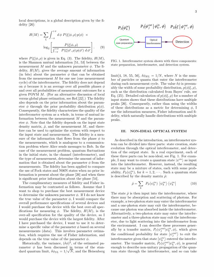
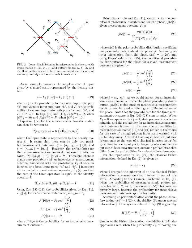
FIG. 2. Lossy Mach-Zehnder interferometer is shown, withinput modes a1, a2, v1, v2, and output modes b1, b2, d1 andd2. Here modes v1 and v2 have vacuum input and the outputmodes d1 and d2 are loss channels in each arm.

As an example, consider the simplest case of inputgiven by a mixed state represented by the density ma-trix

ρ = P0 |0〉 〈0|+ P1 |10〉 〈10| (19)

where P1 is the probability for 1-photon input into port“a” and vacuum input into port “b”, and P0 is the prob-ability of vacuum input into both ports “a” and “b”, andP0 + P1 = 1. In Eqs. (10) and (11), PS(ψ

in) = Po when∣

∣ψin⟩

= |0〉 and PS(ψin) = P1 when

∣

∣ψin⟩

= |10〉.Equation (17) for the interferometer transfer matrix

can then be written as

P (nc, nd|φ, ρ) = tr(

ρ Πφ (nc, nd))

(20)

where the input state is represented by the density ma-trix ρ. It seems that there can be only two possi-ble measurement outcomes, ξ = {nc, nd} = {1, 0} andξ = {nc, nd} = {0, 1}. However, the probabilities forthe two measurement outcomes do not sum to unity be-cause, P (10|φ, ρ) + P (01|φ, ρ) = P1. Therefore, there isa non-zero probability of an inconclusive measurementoutcome associated with the probability P0 of vacuuminjected into both input ports “a” and “b”. I introducean inconclusive measurement operator, Πφ (i), so thatthe sum of the three operators is equal to the identityoperator I:

Πφ (10) + Πφ (01) + Πφ (i) = I (21)

Using Eqs.(18)–(21), the probabilities given by Eq. (11),P (ξ|φ), for measurement outcomes ξ are given by

P (10|φ) = P1 cos2

(

φ

2

)

(22)

P (01|φ) = P1 sin2

(

φ

2

)

(23)

P (i|φ) = 1− P1 (24)

where P (i|φ) is the probability for an inconclusive mea-surement outcome.

Using Bayes’ rule and Eq. (11), we can write the con-ditional probability distributions for the phase, p(φ|ξ),given measurement outcome, ξ, as

p(φ|ξ) = P (ξ|φ) p(φ)+π∫

−π

P (ξ|φ′) p(φ′) dφ′(25)

where p(φ) is the prior probability distribution specifyingour prior information about the phase φ. Assuming noprior information about the phase, p(φ) = 1/(2π), andusing Bayes’ rule in Eq. (25), the conditional probabil-ity distributions for the phase for a given measurementoutcome are given by

p(φ|10) = 1

πcos2

(

φ

2

)

(26)

p(φ|01) = 1

πsin2

(

φ

2

)

(27)

p(φ|i) = 1

2π(28)

where ξ = (nc, nd). As we would expect, for an inconclu-sive measurement outcome the phase probability distri-bution, p(φ|i), is flat since an inconclusive measurementresult cannot be used to distinguish different values ofthe phase. Note that the probabilities for the three mea-surement outcomes in Eq. (26)–(28) sum to unity. WhenP0 = 0, or equivalently P1 = 1, state preparation is deter-ministic, and the probability for an inconclusive measure-ment outcome is zero. In this case, the probabilities formeasurement outcomes (10) and (01) reduce to the valuesfor the case of a single-photon input state created withprobability unity. Note that this single photon input casecorresponds to the case of a classical interferometer fedby a laser in one input port. Larger photon-number in-put states have measurement outcome probabilities thatdiffer from the probabilities for a classical interferometer.For the input state in Eq. (19), the classical Fisher

information, defined in Eq. (2), is given by

F (φ) = P1 (29)

where I dropped the subscript cl on the classical Fisherinformation, a convention that I follow in rest of thiswork. According to the Cramer-Rao bound in Eq. (1),when the probability of creating a single photon ap-proaches zero, P1 → 0, the variance (δφ)2 becomes ar-bitrarily large, because the probability for inconclusivemeasurement outcomes approaches unity.Assuming no prior information about the phase, there-

fore taking p(φ) = 1/(2π), the fidelity (Shannon mutualinformation) of the system defined in Eq. (9) is given by

H(M) = P1

(

1

ln 2− 1

)

(30)

Similar to the Fisher information, the fidelity H(M) alsoapproaches zero when the probability P1 of having one

6

photon in the input of each shot approaches zero. The fi-delity is the amount of information (in bits) that is gainedon average about the phase from a single use of the in-terferometer, averaged over all possible phase values φ.

B. Lossy Mach-Zehnder Interferometer

Next, I consider an interferometer with absorptionlosses—so state evolution is non-unitary. I assume thatstate preparation is deterministic (ideal) and that statedetection is perfect (no errors). Equation (11) is gen-eral enough to describe processes other than losses in theinterferometer, such as photons scattering into the inter-ferometer from the environment, in which case there aremore photons leaving the output ports than entering theinput ports. However, in what follows, I restrict myselfto simple absorption in the interferometer. I model lossesin each arm of a Mach-Zehnder interferometer by insert-ing two beam splitters, S3 and S4, one in each path, seeFig. 2. While a lossless Mach-Zehnder interferometer hastwo input and two output ports, a general lossy Mach-Zehnder interferometer can be represented by four input

and four output ports, see Fig. 2. I label the input modesas a1, a2, v1, and v2, where v1, and v2 have vacuum inputand I label the output modes as b1, b2, d1, and d2, whered1, and d2 are the modes where probability amplitude is“dissipated”. I take the phase shifts at the two mirrors,M1 and M2 to be equal to π. Furthermore, I assumethat the interferometer is balanced, so that path lengthssatisfy,

L = l1 + l3 + l5 = l2 + l4 + l6

l = l1 + l3 = l2 + l4 (31)

see Fig. 2. A calculation gives the input and outputmodes related by the 4×4 unitary scattering matrixSij(φ)

b1b2d1d2

=

Sij (φ)

·

a1a2v1v1

(32)

where the phase-dependent scattering matrix is given by

Sij(φ) =

i2e

iLωc

(√

1− r2y − eiφ√

1− r2x

)

− 12e

iLωc

(√

1− r2y + eiφ√

1− r2x

)

i√2rx e

i(L−l)ωc

1√2ry e

i(L−l)ωc

− 12e

iLωc

(√

1− r2y + eiφ√

1− r2x

)

− i2e

iLωc

(√

1− r2y − eiφ√

1− r2x

)

1√2rx e

i(L−l)ωc

i√2ry e

i(L−l)ωc

− i√2rx e

i(φ+ lωc ) − 1√

2rx e

i(φ+ lωc ) −i

√

1− r2x 0

− 1√2ry e

i lωc − i√

2ry e

i lωc 0 −i

√

1− r2y

(33)

It is easy to check that the scattering matrix is unitary,S† S = I where I is the 4×4 unit matrix. The parame-ters, rx and ry, are the reflection amplitudes for beamssplitters S3 and S4, respectively, and they represent thestrength of the loss or dissipation, see Fig. 2. When thesystem is considered in terms of two input modes, a1 anda2, and two output modes, b1 and b2, the evolution of theinput state in not unitary.

The 4×4 unitary scattering matrix Sij(φ) has somesimple properties. The case when rx = ry = 0 corre-sponds to no dissipation. In this case, the 4×4 S-matrixreduces to two diagonal 2×2 blocks. The upper left 2×2block couple modes a1 and a2 to modes b1 and b2, andthis 2×2 block (up to a phase) is given by Eq. (16), whichis the scattering matrix for the Mach-Zehnder interferom-eter with no losses. For this case of no loss, in Eq. (33)the lower right 2×2 block couples the dissipative modes,d1, and d2, to the vacuum modes, v1, and v2.

The case rx = ry = 1 corresponds to maximum dissi-pation, and the 4×4 S-matrix again decouples, into twooff-diagonal 2×2 blocks. The upper right 2×2 block cou-ples the two vacuum modes, v1 and v2, to the two out-put modes, b1 and b2. The lower left 2×2 block of this

S-matrix couples the loss modes, d1, and d2, to the inputmodes a1 and a2. For this case of maximum dissipation,the input modes, a1 and a2, are decoupled from the out-put modes, b1 and b2.The probabilities for various measurement outcomes

ξ = (n,m) are given by the analog of Eq. (3):

P (n,m|φ, ρ) = tr(

ρo Πφ(n,m))

(34)

where n and m are the number of photons leaving portsb1 and b2, respectively. The trace is over the com-plete space of four direct product Fock basis states,|n1〉a1

⊗ |n2〉a2⊗ |n3〉v1 ⊗ |n4〉v2 . The input state den-

sity matrix, ρo, is defined in terms of a sum of products

of creation operators a†1, a†2, v

†1 and v†2 acting on the vac-

uum |0〉 = |0〉a1⊗ |0〉a2

⊗ |0〉v1 ⊗ |0〉v2 and has the form

ρ0 =∑

n,m

cnm |nm00〉 〈nm00| (35)

where I use the short-hand notation|nm00〉 ≡ |n〉a1

⊗ |m〉a2⊗ |0〉v1 ⊗ |0〉v2 . I am using

the Heisenberg picture, so the input density matrix

7

ρo is independent of time (phase), while the operators

Πφ (n,m) evolve in time (phase) and so they depend on

φ. The projective measurement operators are given by

Πφ (n,m) =1

n!m!

∞∑

k,l=0

1

k! l!

(

b†1

)n (

b†2

)m (

d†1

)k (

d†2

)l

|0〉 〈0|(

b1

)n (

b2

)m (

d1

)k (

d2

)l

(36)

where b†1, b†2, d

†1, and d†2 are creation operators for the

output modes b1, b2, d1, and d2, respectively. The sumsover k and l take into account the probabilities for loos-ing photons into ports d1 and d2. I use the short-handnotation for the input modes {αi} = {a1, a2, v1, v2} and

for the output modes {βi} = {b1, b2, d1, d2}, see Eq. (15).Note that, even though dissipation is being modeled,

it is easy to check that there is global photon numberconservation,

4∑

i=0

α†i αi =

4∑

i=0

β†i βi (37)

since the S-matrix in Eq. (33) is unitary. The measure-ment outcomes, ξ = (n,m), are specified by two integers,which label the number of photons that are output atports b1 and b2, see Fig. 2. So the probability of outputstate, ψout

j , as given in Eq.(34), is expressed by the twointegers n and m, see also Eq. (17). Note that in generalthe number of photons n +m in the output state, ψout

j ,is not equal to the number of photons in the input state,ψin, because

a†1a1 + a†2a2 6= b†1b1 + b†2b2 (38)

However, the sum of probabilities for all possible mea-surement outcomes is unity:

∞∑

m,n=0

P (n,m|φ, ρ) = 1 (39)

where P (n,m|φ, ρ) is given by Eq. (34), and is a resultof

∑

n,m

Πφ (n,m) = I (40)

For the case of a pure input state, |ψin〉, it is convenientto define the operators

N (n,m, k, l) =1

n!m! k! l!

(

b1

)n (

b2

)m (

d1

)k (

d2

)l

(41)and the probabilities in Eq. (34) are then given by

P (n,m|φ, ψin) =

∞∑

k,l=1

∣

∣

∣〈0| N (n,m, k, l) |ψin〉∣

∣

∣

2

(42)

Equation (34), or Eq. (42) for the case of pure states,defines a unitary mapping, |nm00〉 → |n′m′kl〉, be-tween interferometer input states, |nm00〉, and outputstates, |n′m′kl〉, because the photon number is conserved:n+m = n′ +m′ + k + l, see Eq. (37).If we restrict our attention to measurement out-

comes projected onto the Hilbert subspace with basis|n′〉b1 ⊗ |m′〉b2 , Eq. (34) or Eq. (42) defines the non-unitary mapping E :

E[

|n〉a1⊗ |m〉a2

]

→ |n′〉b1 ⊗ |m′〉b2 (43)

since photon number is not conserved: n+m 6= n′ +m′,see Eq. (38), which represents losses in the Mach-Zehnderinterferometer. Here the Fock states |n′〉bi , for i = 1, 2,are created from the vacuum state, |0〉bi , by application

of creation operators b†i in the usual way. The mappingE depends on two parameters, rx and ry, which specifythe strength of the dissipation or losses in each arm ofthe interferometer. In the limit of no dissipation, whenrx = 0 and ry = 0, the mapping E becomes a unitarytransformation and n+m = n′ +m′.In what follows, I use the short-hand notation |nm〉 for

the input state |nm00〉 ≡ |n〉a1 ⊗ |m〉a2 ⊗ |0〉v1 ⊗ |0〉v2 .In the next two subsections, III C and IIID, I discuss

the Fisher information and the fidelity (Shannon mutualinformation) for specific cases of few-photon Fock stateand N00N state input into the lossy Mach-Zehnder (MZ)interferometer.

C. Fock State Input into Lossy MZ Interferometer

Consider the N -photon Fock state

|ψN 〉 = 1√N !

(

a†1

)N

|0〉 = |N000〉 ≡ |N0〉 (44)

input into a lossy Mach-Zehnder interferometer given bythe scattering matrix in Eq. (33). The probabilities formeasurement outcomes ξ = (n,m) are given by:

P (n,m|φ, ψN ) =N !

n!m!

N∑

k=0

N∑

l=0

1

k!l!×

∣

∣Sn11S

m21S

k31S

l41

∣

∣

2δn+m+k+l,N (45)

where Sij are the matrix elements of Eq. (33) and δm,n

is the Kronecker delta function.

8

A direct calculation of the classical Fisher informationfor the N -photon Fock state input, FN (φ), gives

FN (φ) = NF1(φ) (46)

where F1(φ) is the classical Fisher information for one-photon input, given in Eq. (53). This shows that forthe lossy MZ interferometer with N -photon Fock stateinput, the standard deviation (δφ) scales as 1/

√N . From

another point of view, since the Fisher information isadditive for independent events, the N -photon Fock stateacts like N independent 1-photon states. When rx = ry,then F1(φ) = 1, and the N -photon Fisher informationbecomes FN (φ) = N . This means that dissipation in the(non-unitary) interferometer has the effect of introducinga phase dependence into the Fisher information, see thediscussion below.

1. 1-Photon Fock State Input into Lossy MZ Interferometer

As the simplest example of the effect of dissipa-tion, I consider the 1-photon Fock state input into thelossy Mach-Zehnder interferometer with scattering ma-trix given by Eq. (33)

|ψin〉 = a†1 |0〉 = |1000〉 ≡ |10〉 (47)

where I use the short-hand notation |10〉 for the inputstate |1000〉. The probabilities for measurement out-comes are given by P (n,m|φ, ψin), where n,m specifythe photon numbers output in port b1 and b2, respec-tively, see Fig. 2. The probabilities P (n,m|φ, ψin) forthe three measurement outcomes are:

P (10|φ, 10) = 1

4

(

2− r2x − r2y − 2√

(1− r2x)(

1− r2y)

cos φ)

P (01|φ, 10) = 1

4

(

2− r2x − r2y + 2√

(1− r2x)(

1− r2y)

cos φ)

P (00|φ, 10) = 1

2

(

r2x + r2y)

(48)

The probability P (00|φ, 10) is associated with an incon-clusive measurement outcome, since for this case zerophotons leave the output ports, i.e., the photon that en-tered in port “a” was absorbed in the interferometer, ormore precisely the photon was output in either port d1or d2.From Bayes’ rule in Eq. (25), the phase probability

distributions, p(φ|mn,ψin), for input state |ψin〉 givenin Eq. (47), are given by

p(φ|10, 10) = 12π

2−r2x−r2y−2√

(1−r2x)(1−r2y) cosφ

2−r2x−r2y

p(φ|01, 10) = 12π

2−r2x−r2y+2√

(1−r2x)(1−r2y) cosφ

2−r2x−r2y

p(φ|00, 10) = 12π

(49)

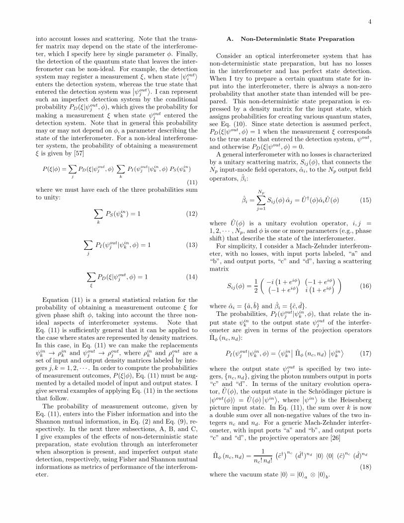
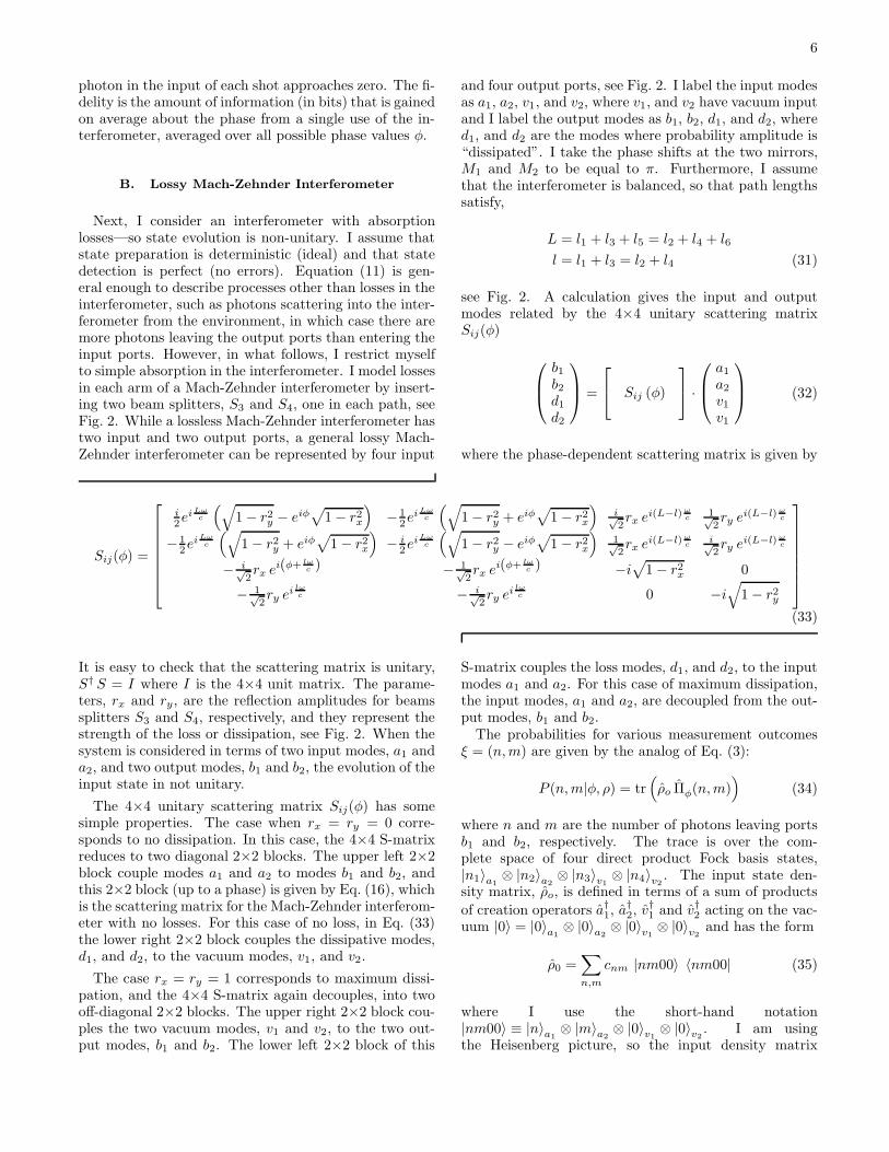
When rx 6= ry, there is a loss of contrast in the phaseprobability distributions p(φ|mn,ψin), see Fig. 3. Whenthe absorption probabilities are the same in both arms,in the limit rx = ry, the phase probability distributions

rx=1.0

0.98

0.95

0.900.0

-3 -2 -1 0 1 2 30.00

0.05

0.10

0.15

0.20

0.25

0.30

Φ

PHΦÈ1

0LpHΦ

10,1

0L

FIG. 3. For the 1-photon input state |10〉, given by Eq. (47),the probability distribution for the phase, p(φ|10, 10), inEq. (49) is plotted for absorption ry = 0 and rx =0.0, 0.90,0.95, 0.98, and 1.0. As rx →1.0, the probability distributionbecomes flat and does not distinguish between different phasevalues.

in Eq. (49) reduce to the case of a single photon inputwithout losses in the interferometer, which are given inEq. (26)-(28), with trivial phase change given by the re-placements sin → cos. The phase probability density,p(φ|00, 10), is associated with the inconclusive outcome,p(φ|i). It is a remarkable feature that for equal lossin both arms, rx = ry, the phase probability densities,p(φ|mn,ψin), in Eq.(49) do not depend on the size ofthe loss, rx. However, there is loss of information withincreasing absorption, rx and ry, which is reflected in theinformation measures, see below.The effect of equal dissipation in both arms of the in-

terferometer is the same as the effect of non-deterministicstate preparation, specified by input state characterizedby a density matrix in Eq. (19). However, when the dis-sipation in both arms is not equal, say for ry = 0 and rxis finite, the phase probability distributions show a lossof contrast, see Fig. 3. This feature may be useful inapplications to null-type measurements.In the discussion that follows, I assume no prior infor-

mation on the phase, so I take p(φ) = 1/(2π). Whenthere is no loss in the interferometer, rx = ry = 0,the Shannon mutual information (fidelity) as defined inEq. (9) is a constant:

H(M) =1

ln 2− 1 (50)

When the losses in both arms are equal, rx = ry, we havethe exact result

H(M) =

(

1

ln 2− 1

)

(

1− r2x)

(51)

For general values of rx and ry, the expression forH(M) is large and complicated, but for small rx ≪ 1and ry ≪ 1, I can expand it in a power series,

H(M) =

(

1

ln 2− 1

)[

1−1

2

(

r2x + r2y)

]

+O(r4x)+O(r4y) (52)

9

rx = ry

ry = 0

0.0 0.2 0.4 0.6 0.8 1.00.0

0.1

0.2

0.3

0.4

rx2

HHFÈML

HHML

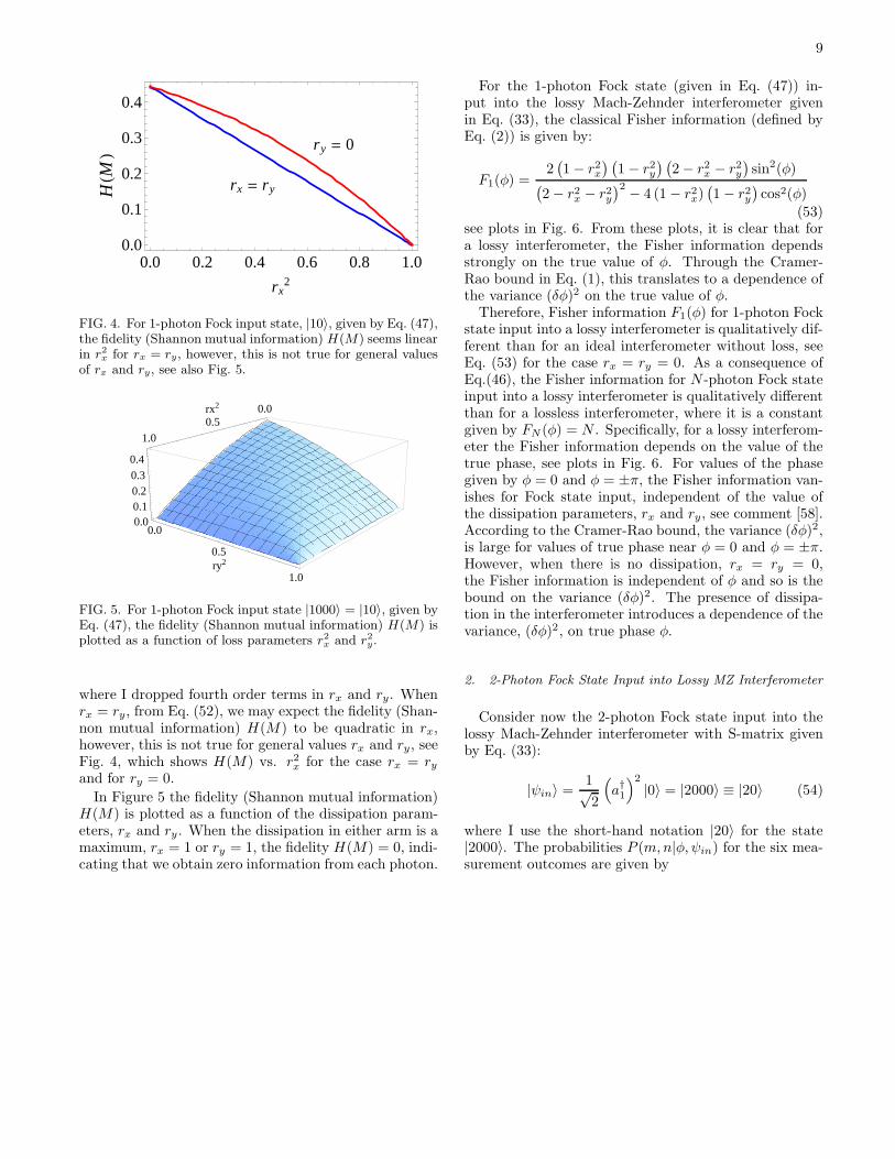
FIG. 4. For 1-photon Fock input state, |10〉, given by Eq. (47),the fidelity (Shannon mutual information) H(M) seems linearin r2x for rx = ry, however, this is not true for general valuesof rx and ry, see also Fig. 5.

0.00.5

1.0

rx2

0.0

0.5

1.0ry2

0.00.10.20.30.4

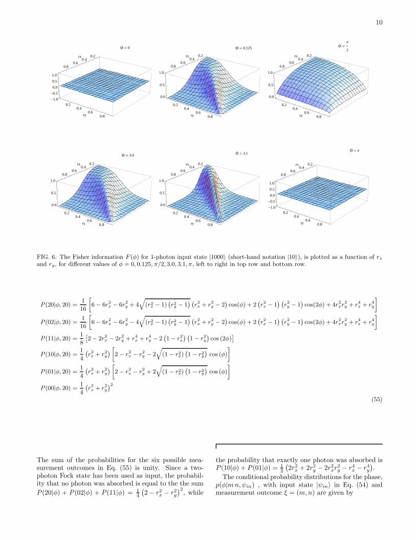
FIG. 5. For 1-photon Fock input state |1000〉 = |10〉, given byEq. (47), the fidelity (Shannon mutual information) H(M) isplotted as a function of loss parameters r2x and r2y.

where I dropped fourth order terms in rx and ry. Whenrx = ry, from Eq. (52), we may expect the fidelity (Shan-non mutual information) H(M) to be quadratic in rx,however, this is not true for general values rx and ry, seeFig. 4, which shows H(M) vs. r2x for the case rx = ryand for ry = 0.

In Figure 5 the fidelity (Shannon mutual information)H(M) is plotted as a function of the dissipation param-eters, rx and ry . When the dissipation in either arm is amaximum, rx = 1 or ry = 1, the fidelity H(M) = 0, indi-cating that we obtain zero information from each photon.

For the 1-photon Fock state (given in Eq. (47)) in-put into the lossy Mach-Zehnder interferometer givenin Eq. (33), the classical Fisher information (defined byEq. (2)) is given by:

F1(φ) =2(

1− r2x) (

1− r2y) (

2− r2x − r2y)

sin2(φ)(

2− r2x − r2y)2 − 4 (1− r2x)

(

1− r2y)

cos2(φ)(53)

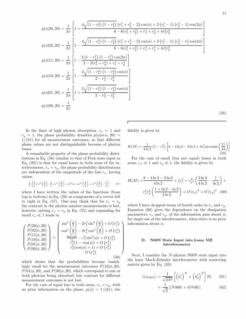
see plots in Fig. 6. From these plots, it is clear that fora lossy interferometer, the Fisher information dependsstrongly on the true value of φ. Through the Cramer-Rao bound in Eq. (1), this translates to a dependence ofthe variance (δφ)2 on the true value of φ.Therefore, Fisher information F1(φ) for 1-photon Fock

state input into a lossy interferometer is qualitatively dif-ferent than for an ideal interferometer without loss, seeEq. (53) for the case rx = ry = 0. As a consequence ofEq.(46), the Fisher information for N -photon Fock stateinput into a lossy interferometer is qualitatively differentthan for a lossless interferometer, where it is a constantgiven by FN (φ) = N . Specifically, for a lossy interferom-eter the Fisher information depends on the value of thetrue phase, see plots in Fig. 6. For values of the phasegiven by φ = 0 and φ = ±π, the Fisher information van-ishes for Fock state input, independent of the value ofthe dissipation parameters, rx and ry, see comment [58].According to the Cramer-Rao bound, the variance (δφ)2,is large for values of true phase near φ = 0 and φ = ±π.However, when there is no dissipation, rx = ry = 0,the Fisher information is independent of φ and so is thebound on the variance (δφ)2. The presence of dissipa-tion in the interferometer introduces a dependence of thevariance, (δφ)2, on true phase φ.

2. 2-Photon Fock State Input into Lossy MZ Interferometer

Consider now the 2-photon Fock state input into thelossy Mach-Zehnder interferometer with S-matrix givenby Eq. (33):

|ψin〉 =1√2

(

a†1

)2

|0〉 = |2000〉 ≡ |20〉 (54)

where I use the short-hand notation |20〉 for the state|2000〉. The probabilities P (m,n|φ, ψin) for the six mea-surement outcomes are given by

10

0.20.4

0.60.8

rx

0.20.4

0.60.8ry

-1.0

-0.5

0.0

0.5

1.0

0.20.4

0.60.8

rx

0.20.4

0.60.8ry

0.0

0.5

1.0

0.20.4

0.60.8

rx

0.20.4

0.60.8ry

0.0

0.5

1.0

0.20.4

0.60.8

rx

0.20.4

0.60.8ry

0.0

0.5

1.0

0.20.4

0.60.8

rx

0.20.4

0.60.8ry

0.0

0.5

1.0

0.20.4

0.60.8

rx

0.20.4

0.60.8ry

-1.0

-0.5

0.0

0.5

1.0

Æ = 0 Æ = 0.125 Æ =Π

2

Æ = 3.0 Æ = 3.1Æ = Π

FIG. 6. The Fisher information F (φ) for 1-photon input state |1000〉 (short-hand notation |10〉), is plotted as a function of rxand ry, for different values of φ = 0, 0.125, π/2, 3.0, 3.1, π, left to right in top row and bottom row.

P (20|φ, 20) =1

16

[

6− 6r2x − 6r2y + 4√

(r2x − 1)(

r2y − 1) (

r2x + r2y − 2)

cos(φ) + 2(

r2x − 1) (

r2y − 1)

cos(2φ) + 4r2xr2

y + r4x + r4y

]

P (02|φ, 20) =1

16

[

6− 6r2x − 6r2y − 4√

(r2x − 1)(

r2y − 1) (

r2x + r2y − 2)

cos(φ) + 2(

r2x − 1) (

r2y − 1)

cos(2φ) + 4r2xr2

y + r4x + r4y

]

P (11|φ, 20) =1

8

[

2− 2r2x − 2r2y + r4x + r4y − 2(

1− r2x) (

1− r2y)

cos (2φ)]

P (10|φ, 20) =1

4

(

r2x + r2y)

[

2− r2x − r2y − 2√

(1− r2x)(

1− r2y)

cos (φ)

]

P (01|φ, 20) =1

4

(

r2x + r2y)

[

2− r2x − r2y + 2√

(1− r2x)(

1− r2y)

cos (φ)

]

P (00|φ, 20) =1

4

(

r2x + r2y)2

(55)

The sum of the probabilities for the six possible mea-surement outcomes in Eq. (55) is unity. Since a two-photon Fock state has been used as input, the probabil-ity that no photon was absorbed is equal to the the sum

P (20|φ) + P (02|φ) + P (11|φ) = 14

(

2− r2x − r2y)2, while

the probability that exactly one photon was absorbed isP (10|φ) + P (01|φ) = 1

2

(

2r2x + 2r2y − 2r2xr2y − r4x − r4y

)

.

The conditional probability distributions for the phase,p(φ|mn,ψin) , with input state |ψin〉 in Eq. (54) andmeasurement outcome ξ = (m,n) are given by

11

p(φ|20, 20) = 1

2π

1 +4√

(1− r2x)(

1− r2y) (

r2x + r2y − 2)

cos(φ) + 2(

r2x − 1) (

r2y − 1)

cos(2φ)

6− 6(r2x + r2y) + r4x + r4y + 4r2xr2y

p(φ|02, 20) = 1

2π

1−4√

(1− r2x)(

1− r2y) (

r2x + r2y − 2)

cos(φ) + 2(

r2x − 1) (

r2y − 1)

cos(2φ)

6− 6(r2x + r2y) + r4x + r4y + 4r2xr2y

p(φ|11, 20) = 1

2π

[

1−2(

1− r2x) (

1− r2y)

cos(2φ)

2− 2(r2x + r2y) + r4x + r4y

]

p(φ|10, 20) = 1

2π

1−2√

(1− r2x)(

1− r2y)

cos(φ)

2− r2x − r2y

p(φ|01, 20) = 1

2π

1 +2√

(1− r2x)(

1− r2y)

cos(φ)

2− r2x − r2y

p(φ|00, 20) = 1

2π(56)

In the limit of high photon absorption, rx = 1 andry = 1, the phase probability densities p(φ|mn, 20) =1/(2π) for all measurement outcomes, so that differentphase values are not distinguishable because of photonlosses.A remarkable property of the phase probability distri-

butions in Eq. (56) (similar to that of Fock state input inEq. (49)) is that for equal losses in both arms of the in-terferometer, rx = ry , the phase probability distributionsare independent of the magnitude of the loss rx, havingvalues

1

π

{

4

3sin

4(

φ

2

)

,4

3cos

4(

φ

2

)

, sin2(φ), sin

2(

φ

2

)

, cos2(

φ

2

)

,1

2

}

(57)

where I have written the values of the functions (fromtop to bottom) in Eq. (56) as components of a vector leftto right in Eq. (57). One may think that for rx = rythe contrast in the photon number measurements is lost,however, setting rx = ry in Eq. (55) and expanding forsmall rx ≪ 1 leads to

P (20|φ, 20)P (02|φ, 20)P (11|φ, 20)P (10|φ, 20)P (01|φ, 20)P (00|φ, 20)

=

sin4(

φ2

)

− 2r2x sin4(

φ2

)

+O(

r4x)

cos4(

φ

2

)

− 2r2x cos4(

φ

2

)

+O(

r4x)

sin2(φ)2 − r2x sin

2(φ) +O(

r4x)

r2x(1− cos(φ)) +O(

r4x)

r2x(cos(φ) + 1) +O(

r4x)

O(

r4x)

(58)which shows that the probabilities become vanish-ingly small for the measurement outcomes P (10|φ, 20),P (01|φ, 20), and P (00|φ, 20), which correspond to one orboth photons being absorbed, but contrast for differentmeasurement outcomes is not lost.For the case of equal loss in both arms, rx = ry, with

no prior information on the phase, p(φ) = 1/(2π), the

fidelity is given by

H(M) =1

4 ln 2

(

1− r2x)

[

8− 4 ln 2− 3 ln 3 + 2r2xarctanh

(

11

43

)]

(59)

For the case of small (but not equal) losses in botharms, rx ≪ 1 and ry ≪ 1, the fidelity is given by

H(M) =8− 4 ln 2− 3 ln 3

4 ln 2+(

r2x + r2y)

(

3 ln 3

4 ln 2− 1

ln 2

)

+

r2xr2y

(

1 + ln 2− ln 3

2 ln 2

)

+O (rx)4+O (ry)

4(60)

where I have dropped terms of fourth order in rx and ry.Equation (60) gives the dependence on the dissipationparameters, rx and ry , of the information gain about φ,for single use of the interferometer, when there is no priorinformation about φ.

D. N00N State Input into Lossy MZ

Interferometer

Next, I consider the N -photon N00N state input intothe lossy Mach-Zehnder interferometer with scatteringmatrix given by Eq. (33):

|ψN00N 〉 = 1√2N !

[

(

a†1

)N

+(

a†2

)N]

|0〉 (61)

=1√2[|N000〉+ |0N00〉] (62)

12

For the input state in Eq. (62), the probability for mea-surement outcome ξ = (n,m) is given by

P (n,m|φ, ψN00N ) =N !

2n!m!

N∑

k=0

N∑

l=0

1

k!l!×

∣

∣Sn11S

m21S

k31S

l41 + Sn

12Sm22S

k32S

l42

∣

∣

2δn+m+k+l,N (63)

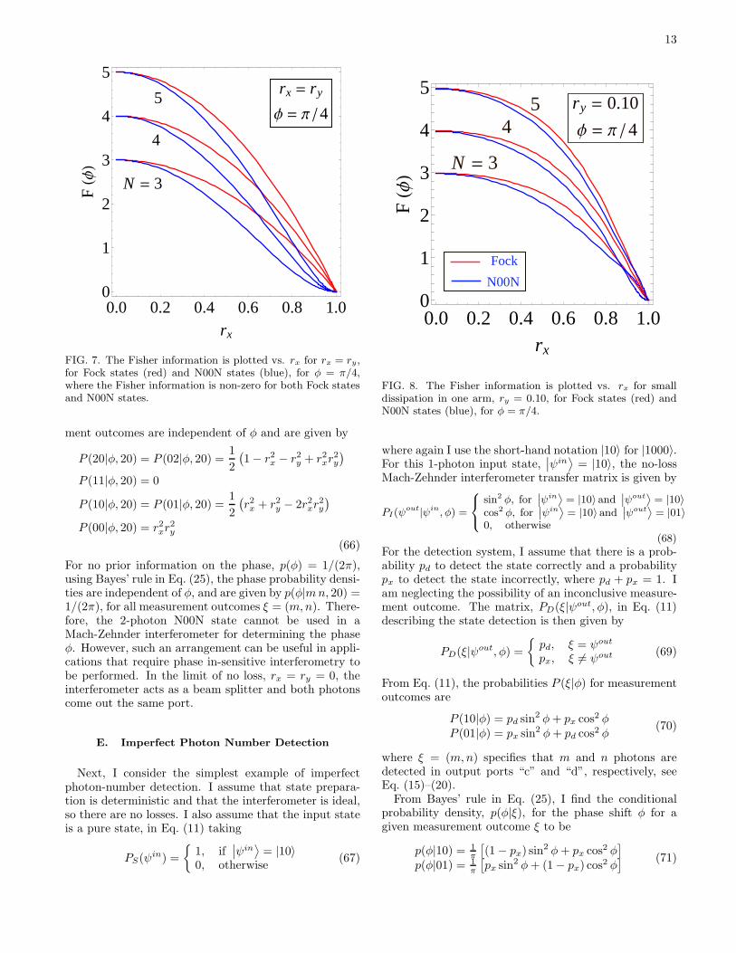
where n and m are the number of photons output inports b1 and b2, respectively. Using the Fisher informa-tion, I compare how well Fock states and N00N statesperform in the presence of absorption losses. In Fig. 7,I plot the classical Fisher information for N =3, 4, and5 photon Fock states and N00N states, plotted vs. rxfor the special case where rx = ry . The plots show that,for equal dissipation in both arms, and for equal photonnumber, Fock states perform better for phase estimationthan N00N states, for the same amount of dissipation rx,see Eq. (1).For N00N states, the Fisher information vanishes at

the phase values: φ = 0,±π/2,±π. While for Fockstates, the Fisher information vanished only at φ = 0,±π.For φ close to these values, phase estimation may havelarge standard deviation, see Eq.(1).Figure 8 shows the classical Fisher information for the

case where Fock and N00N states are input into a Mach-Zehnder interferometer with small dissipation (losses)and when the losses are not equal in both arms. Gen-erally, Fock states perform better (have larger Fisher in-formation) for all values of dissipation rx except at thevery highest values of rx ∼ 0.95. The comparison is madeat a true value of φ = π/4, where the Fisher informationsdo not vanish.Figure 9 shows a plot of the classical Fisher informa-

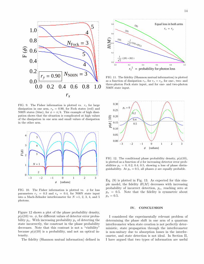
tion for Fock and for N00N states for N = 3, 4 and 5photons for the case of large dissipation in one arm ofthe Mach-Zehnder interferometer, ry = 0.9. The com-parison is complicated, since for the N =3 photon case,Fock states perform better than N00N states for largedissipation rx ∼ 0.8, whereas the situation is reversed forsmall dissipation rx ∼ 0.05.In Figures 8 and 9, the comparisons are made at a true

value of phase φ = π/4, where the classical Fisher infor-mations (for Fock and N00N states) do not vanish. Whendissipation is present, the classical Fisher information hasa complicated behavior as a function of the true phaseφ, see Fig. 10. This shows that phase estimation usingsimple photon counting is a sensitive procedure whoseaccuracy depends on the true value of phase.The classical Fisher information for a lossy Mach-

Zehnder interferometer depends on the true value of thephase φ. The fidelity (Shannon mutual information) isan information measure that averages over all phases, forprior information given by p(φ), see Eq. (9). Figure 11shows a comparison of the fidelity versus dissipation rxfor Fock and N00N states for equal dissipation in botharms, rx = ry. The fidelity of 1-photon Fock and N00Nstates is equal, see the discussion below. For a given

amount of dissipation, rx, for Fock states the fidelity in-creases with input photon number N . The fidelity for2-photon N00N state input is exactly zero for all valuesof dissipation rx because this state carries no informationabout the phase in a Mach-Zehnder interferometer, seethe discussion below.

1. 1-Photon N00N State Input into Lossy MZInterferometer

Consider now the 1-photon entangled N00N state:

∣

∣ψN00N1

⟩

=1√2

(

a†1 + a†2

)

|0〉 = 1√2[|10〉+ |01〉] (64)

where again, I use the short-hand notation |10〉 for |1000〉and |01〉 for |0100〉. The probabilities for the measure-ment outcomes for this input state are given by Eq. (48)with the replacement cosφ→ sinφ. Similarly, the phaseprobability distributions, assuming no prior information,p(φ) = 1/(2π), are given by Eq. (49) with the replace-ment cosφ → sinφ. The fidelity for this input stateis the same as for the 1-photon Fock state, given byEq. (50)–(52). Therefore, according to Shannon mutualinformation (fidelity), the presence of entanglement inthe 1-photon N00N state has not improved the informa-tion on the phase.

The Fisher information for this entangled state is givenby the 1-photon Fock state Fisher information in Eq. (53)with the replacements φ → π

2 − φ. Therefore, the en-tanglement simply has the effect of changing the phaseof the classical Fisher information. This phase changechanges the places where F (φ) = 0, which, for this en-tangled state, is now φ = ±π/2. Comparison of the 1-photon Fock state to the the 1-photon entangled N00Nstate shows that the introduction of entanglement doesnot remove the φ dependence of the Fisher informationwhen losses are present. However, when losses are ab-sent, rx = ry = 0, the Fisher information for input stategiven by Eq. (64) reduces to F (φ) = 1, independent of φ,as in the 1-photon Fock state without losses.

2. 2-Photon N00N State Input into Lossy MZInterferometer

The 2-photon N00N state,

∣

∣ψN00N2

⟩

=1

2

[

(

a†1

)2

+(

a†2

)2]

|0〉 = 1√2[|20 〉+ |02 〉]

(65)has a peculiar behavior when input into a Mach-Zehnderinterferometer with losses. The probabilities distribu-tions, given by Eqs. (42) and (63), for the six measure-

13

N = 3

4

5rx = ry

Φ = Π �4

0.0 0.2 0.4 0.6 0.8 1.00

1

2

3

4

5

rx

FHΦL

FIG. 7. The Fisher information is plotted vs. rx for rx = ry,for Fock states (red) and N00N states (blue), for φ = π/4,where the Fisher information is non-zero for both Fock statesand N00N states.

ment outcomes are independent of φ and are given by

P (20|φ, 20) = P (02|φ, 20) = 1

2

(

1− r2x − r2y + r2xr2y

)

P (11|φ, 20) = 0

P (10|φ, 20) = P (01|φ, 20) = 1

2

(

r2x + r2y − 2r2xr2y

)

P (00|φ, 20) = r2xr2y

(66)

For no prior information on the phase, p(φ) = 1/(2π),using Bayes’ rule in Eq. (25), the phase probability densi-ties are independent of φ, and are given by p(φ|mn, 20) =1/(2π), for all measurement outcomes ξ = (m,n). There-fore, the 2-photon N00N state cannot be used in aMach-Zehnder interferometer for determining the phaseφ. However, such an arrangement can be useful in appli-cations that require phase in-sensitive interferometry tobe performed. In the limit of no loss, rx = ry = 0, theinterferometer acts as a beam splitter and both photonscome out the same port.

E. Imperfect Photon Number Detection

Next, I consider the simplest example of imperfectphoton-number detection. I assume that state prepara-tion is deterministic and that the interferometer is ideal,so there are no losses. I also assume that the input stateis a pure state, in Eq. (11) taking

PS(ψin) =

{

1, if∣

∣ψin⟩

= |10〉0, otherwise

(67)

54

N = 3

Fock

N00N

ry = 0.10

Φ = Π � 4

0.0 0.2 0.4 0.6 0.8 1.00

1

2

3

4

5

rx

FHΦL

FIG. 8. The Fisher information is plotted vs. rx for smalldissipation in one arm, ry = 0.10, for Fock states (red) andN00N states (blue), for φ = π/4.

where again I use the short-hand notation |10〉 for |1000〉.For this 1-photon input state,

∣

∣ψin⟩

= |10〉, the no-lossMach-Zehnder interferometer transfer matrix is given by

PI(ψout|ψin, φ) =

sin2 φ, for∣

∣ψin⟩

= |10〉 and∣

∣ψout⟩

= |10〉cos2 φ, for

∣

∣ψin⟩

= |10〉 and∣

∣ψout⟩

= |01〉0, otherwise

(68)

For the detection system, I assume that there is a prob-ability pd to detect the state correctly and a probabilitypx to detect the state incorrectly, where pd + px = 1. Iam neglecting the possibility of an inconclusive measure-ment outcome. The matrix, PD(ξ|ψout, φ), in Eq. (11)describing the state detection is then given by

PD(ξ|ψout, φ) =

{

pd, ξ = ψout

px, ξ 6= ψout (69)

From Eq. (11), the probabilities P (ξ|φ) for measurementoutcomes are

P (10|φ) = pd sin2 φ+ px cos

2 φP (01|φ) = px sin

2 φ+ pd cos2 φ

(70)

where ξ = (m,n) specifies that m and n photons aredetected in output ports “c” and “d”, respectively, seeEq. (15)–(20).From Bayes’ rule in Eq. (25), I find the conditional

probability density, p(φ|ξ), for the phase shift φ for agiven measurement outcome ξ to be

p(φ|10) = 1π

[

(1− px) sin2 φ+ px cos

2 φ]

p(φ|01) = 1π

[

px sin2 φ+ (1− px) cos

2 φ] (71)

14

ry = 0.90 NN00N = 3

4

5

NFock = 3

45

0.0 0.2 0.4 0.6 0.8 1.00.0

0.2

0.4

0.6

0.8

1.0

rx

FHΦL

FIG. 9. The Fisher information is plotted vs. rx for largedissipation in one arm, ry = 0.90, for Fock states (red) andN00N states (blue), for φ = π/4. This example of high dissi-pation shows that the situation is complicated at high valuesof the dissipation in one arm and small values of dissipationin the other arm.

N = 1

2

3

4

5

-3 -2 -1 0 1 2 30

1

2

3

4

Φ @radiansD

FN

00NHΦL

FHΦL

FIG. 10. The Fisher information is plotted vs. φ for lossparameters rx = 0.3 and ry = 0.4, for N00N state inputinto a Mach-Zehnder interferometer for N =1, 2, 3, 4, and 5photons.

Figure 12 shows a plot of the phase probability density,p(φ|10) vs. φ, for different values of detector error proba-bility px. With increasing probability px of detecting thestate incorrectly, the constrast in the phase probabilitydecreases. Note that this contrast is not a “visibility”because p(φ|10) is a probability, and not an optical in-tensity.

The fidelity (Shannon mutual information) defined in

1

2H  20\ +  02\ L

 10\

 20\

1

2H 10\+ 01\L

 30\

0.0 0.2 0.4 0.6 0.8 1.0

0.0

0.2

0.4

0.6

0.8 Equal loss in both arms

rx = ry

rx2 = probability for photon loss

HHML

FIG. 11. The fidelity (Shannon mutual information) is plottedas a function of dissipation rx, for rx = ry, for one-, two- andthree-photon Fock state input, and for one- and two-photonN00N state input.

px = 0

0.2

0.4

0.5

-3 -2 -1 0 1 2 30.00

0.05

0.10

0.15

0.20

0.25

0.30

Φ @radiansD

PHΦÈ1

,0L

1-photon input in port a

pHΦ

10L

FIG. 12. The conditional phase probability density, p(φ|10),is plotted as a function of φ for increasing detector error prob-abilities px = 0, 0.2, 0.4, 0.5, showing a loss of phase distin-guishability. At px = 0.5, all phases φ are equally probable.

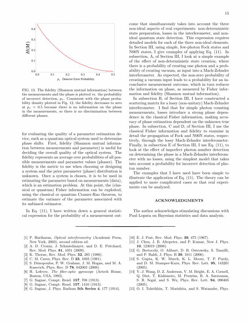
Eq. (9) is plotted in Fig. 13. As expected for this sim-ple model, the fidelity H(M) decreases with increasingprobability of incorrect detection, px, reaching zero atpx = 0.5. Note that the fidelity is symmetric aboutpx = 0.5.

IV. CONCLUSION

I considered the experimentally relevant problem ofdetermining the phase shift in one arm of a quantuminterferometer when state creation is not perfectly deter-ministic, state propagation through the interferometeris non-unitary due to absorption losses in the interfer-ometer, and state detection is not ideal. In Section II,I have argued that two types of information are useful

15

0.0 0.1 0.2 0.3 0.4 0.50.0

0.1

0.2

0.3

0.4

px Detector Error Probability

HHΦÈML

Mutual information vs. Detecor Error Probability

HHML

FIG. 13. The fidelity (Shannon mutual information) betweenthe measurements and the phase is plotted vs. the probabilityof incorrect detection, px. Consistent with the phase proba-bility density plotted in Fig. 12, the fidelity decreases to zeroat px = 0.5 because there is no information on the phasein the measurements, so there is no discrimination betweendifferent phases.

for evaluating the quality of a parameter estimation de-vice, such as a quantum optical system used to determinephase shifts. First, fidelity (Shannon mutual informa-tion between measurements and parameter) is useful fordeciding the overall quality of the optical system. Thefidelity represents an average over probabilities of all pos-sible measurements and parameter values (phases). Thefidelity is the metric to use when choosing or designinga system and the prior parameter (phase) distribution isunknown. Once a system is chosen, it is to be used inestimating the parameter based on measurements (data),which is an estimation problem. At this point, the (clas-sical or quantum) Fisher information can be exploited,using the classical or quantum Cramer-Rao theorem, toestimate the variance of the parameter associated withits unbiased estimator.

In Eq. (11), I have written down a general statisti-cal expression for the probability of a measurement out-

come that simultaneously takes into account the threenon-ideal aspects of real experiments: non-deterministicstate preparation, losses in the interferometer, and non-ideal quantum state detection. This expression requiresdetailed models for each of the three non-ideal elements.In Section III, using simple, few-photon Fock states andN00N states, I give examples of applying Eq. (11). Insubsection, A, of Section III, I look at a simple exampleof the effect of non-deterministic state creation, wherethere is a probability of creating one photon and a prob-ability of creating vacuum, as input into a Mach-Zehnderinterferometer. As expected, the non-zero probability ofcreating a vacuum input leads to a probability for an in-conclusive measurement outcome, which in turn reducesthe information on phase, as measured by Fisher infor-mation and fidelity (Shannon mutual information).In subsection B, of Section III, I have constructed a

scattering matrix for a lossy (non-unitary) Mach-Zehnderinterferometer. I find that for simple photon countingmeasurements, losses introduce a strong phase depen-dence in the classical Fisher information, making accu-racy of phase estimation dependent on the unknown truephase. In subsection, C and D, of Section III, I use theclassical Fisher information and fidelity to examine indetail the propagation of Fock and N00N states, respec-tively, through the lossy Mach-Zehnder interferometer.Finally, in subsection E of Section III, I use Eq. (11), tolook at the effect of imperfect photon number detectionon determining the phase in a Mach-Zehnder interferom-eter with no losses, using the simplest model that takesinto account a probability for incorrect detection of pho-ton number.The examples that I have used have been simple to

illustrate the application of Eq. (11). The theory can beapplied to more complicated cases so that real experi-ments can be analyzed.

ACKNOWLEDGMENTS

The author acknowledges stimulating discussions withPaul Lopata on Bayesian statistics and data analysis.

[1] P. Hariharan, Optical interferometry (Academic Press,New York, 2003), second edition ed.

[2] A. D. Cronin, J. Schmiedmayer, and D. E. Pritchard,Rev. Mod. Phys. 81, 1051 (2009).

[3] K. Thorne, Rev. Mod. Phys. 52, 285 (1980).[4] C. M. Caves, Phys. Rev. D 23, 1693 (1981).[5] S. Dimopoulos, P. W. Graham, J. M. Hogan, and M. A.

Kasevich, Phys. Rev. D 78, 042003 (2008).[6] H. Lefevre, The fiber-optic gyroscope (Artech House,

Boston, USA, 1993).[7] G. Sagnac, Compt. Rend. 157, 708 (1913).[8] G. Sagnac, Compt. Rend. 157, 1410 (1913).[9] G. Sagnac, J. Phys. Radium 5th Series 4, 177 (1914).

[10] E. J. Post, Rev. Mod. Phys. 39, 475 (1967).[11] J. Chen, J. B. Altepeter, and P. Kumar, New J. Phys.

10, 123019 (2008).[12] G. Bertocchi, O. Alibart, D. B. Ostrowsky, S. Tanzilli,

and P. Baldi, J. Phys. B 39, 1011 (2006).[13] S. Gupta, K. W. Murch, K. L. Moore, T. P. Purdy,

and D. M. Stamper-Kurn, Phys. Rev. Lett. 95, 143201(2005).

[14] Y.-J. Wang, D. Z. Anderson, V. M. Bright, E. A. Cornell,Q. Diot, T. Kishimoto, M. Prentiss, R. A. Saravanan,S. R. Segal, and S. Wu, Phys. Rev. Lett. 94, 090405(2005).

[15] O. I. Tolstikhin, T. Morishita, and S. Watanabe, Phys.

16

Rev. A 72, 051603(R) (2005).[16] J. J. Cooper, D. W. Hallwood, and J. A. Dunningham,

Phys. Rev. A 81, 043624 (2010).[17] R. M. Godun, M. B. d’Arcy, G. S. Summy, and K. Bur-

nett, Contemporary Physics 42, 77 (2001).[18] V. Giovannetti, S. Lloyd, and L. Maccone, Phys. Rev.

Lett. 96, 010401 (2006).[19] D. W. Berry, B. L. Higgins, S. D. Bartlett, M. W.

Mitchell, G. J. Pryde, and H. M. Wiseman, Phys. Rev.A 80, 052114 (2009).

[20] J. Combes and H. M. Wiseman, J. Opt. B: QuantumSemiclass 7, 14 (2005).

[21] T. Nagata, R. Okamoto, J. L. O’Brien, K. Sasaki, andS. Takeuchi, Science 316, 726 (2007).

[22] G. A. Durkin and J. P. Dowling, Phys. Rev. Lett. 99,070801 (2007).

[23] L. Pezze and A. Smerzi, Phys. Rev. Lett. 100, 073601(2008).

[24] U. Dorner, R. Demkowicz-Dobrzanski, B. J. Smith, J. S.Lundeen, W. Wasilewski, K. Banaszek, and I. A. Walm-sley, Phys. Rev. Lett. 102, 040403 (2009).

[25] H. Cable and G. A. Durkin, Phys. Rev. Lett. 105, 013603(2010).

[26] T. B. Bahder and P. A. Lopata, Phys.Rev. A 74, 051801R (2006), URLhttp://arxiv.org/abs/quant-ph/0602123.

[27] H. Cramer, Mathematical Methods of Statistics (Prince-ton University Press, Princeton, 1958), eight printing.

[28] C. W. Helstrom, Phys. Lett. A 25, 101 (1967).[29] C. W. Helstrom, Quantum Detection and Estimation

Theory (Academic Press, New York, 1976).[30] A. S. Holevo, Probabilistic and Statistical Aspects of

Quantum Theory (North-Holland, Amsterdam, 1982).[31] S. L. Braunstein and C. M. Caves, Phys. Rev. Lett. 72,

3439 (1994).[32] S. L. Braunstein, C. M. Caves, and G. J. Milburn, Ann.

of Phys. 247, 135 (1996).[33] O. E. Barndorff-Nielsen and R. D. Gill, J. Phys. A: Math.

Gen. 33, 4481 (2000).[34] O. E. Barndorff-Nielsen, R. D. Gill, and P. E.

Jupp, J. Roy. Stat. Soc. B 65, 775 (2003), URLhttp://arxiv.org/abs/quant-ph/0307191.

[35] P. Walther, J. Pan, M. Aspelmeyer, R. Ursin, S. Gaspa-roni, and A. Zeilinger, Nature 429, 158 (2004).

[36] M. W. Mitchell, J. S. Lundeen, and A. M. Steinberg,Nature 429, 161 (2004).

[37] R. Okamoto, H. F. Hofmann, T. Nagata, J. L. O’Brien,K. Sasaki, and S. Takeuchi, New J. Phys. 10, 073033(2008).

[38] M. Kacprowicz, R. Demkowicz-Dobrzanski,W. Wasilewski, K. Banaszek, and I. A. Walm-sley, Nature Photonics 4, 357 (2010), URLhttp://lanl.arxiv.org/abs/0906.3511.

[39] N. Thomas-Peter, B. J. Smith, and I. A. Walmsley, inLasers and Electro-Optics, 2009 and 2009 Conferenceon Quantum electronics and Laser Science Conference.CLEO/QELS 2009. (Baltimore, MD, 2009), pp. 978–1–55752–869–8.

[40] T. Kim, O. Pfister, M. J. Holland, J. Noh, and J. L. Hall,Phys. Rev. A 57, 4004 (1998).

[41] G. A. Durkin, C. Simon, J. Eisert, and D. Bouwmeester,Phys. Rev. A 70, 062305 (2004).

[42] M. A. Rubin and S. Kaushik, Phys. Rev. A 75, 053805(2007).

[43] G. Gilbert, M. Hamrick, and Y. S. Weinstein, J. Opt.Soc. Am. B 25, 1336 (2008).

[44] R. Demkowicz-Dobrzanski, U. Dorner, B. J. Smith, J. S.Lundeen, W. Wasilewski, K. Banaszek, and I. A. Walm-sley, Phys. Rev. A 80, 013825 (2009).

[45] T. Ono and H. F. Hofmann, Phys. Rev. A 81, 033819(20010).

[46] G. M. DAriano, M. G. A. Paris, and M. F. Sacchi, Phys.Rev. A 62, 023815 (2000).

[47] A. Monras, Phys. Rev. A 73, 033821 (2006).[48] S. Olivares and M. G. A. Paris, J. Phys. B 42, 055506

(2009).[49] R. Gaiba and M. G. A. Paris, Phys. Lett. A 373, 934

(2009).[50] B. L. Higgins, D. W. Berry, S. D. Bartlett, M. W.

Mitchell, H. M. Wiseman, and G. J. Pryde, New J. Phys.11, 073023 (2009).

[51] T. M. Cover and J. A. Thomas, Elements of InformationTheory (J. Wiley & Sons, Inc., Hoboken, New Jersey,2006), second edition ed.

[52] H. F. Hofmann, Phys. Rev. A 79, 033822 (2009).[53] C. E. Shannon, The Bell System Technical Journal 27,

379 (1948).[54] T. B. Bahder and P. A. Lopata, in The 8th International

Conference on Quantum Communication, Measurement,and Computing (Tsukuba, Japan, 2006), pp. 369–372,URL http://xxx.lanl.gov/abs/quant-ph/0701243.

[55] Z. Y. Ou, Phys. Rev. A 55, 2598 (1997).[56] V. Giovannetti, S. Lloyd, and L. Maccone, Science 306,

1330 (2004).[57] E. T. Jaynes, Probability Theory the Logic of Science

(Cambridge Press, Cambridge, UK, 2009), sixth print-ing.

[58] Note1, this statement applies to a balanced interferome-ter, whose path lengths satisfy Eq. (31).