Embed Size (px)
Citation preview
Expander 6.2 Online Documentation
Introduction ......................................................................................................... 1 Starting EXPANDER ........................................................................................... 2 Input Data ........................................................................................................... 3 Tabular Data File ................................................................................................ 3 CEL Files ........................................................................................................... 5 Working on similarity data no associated expression data .................................. 7 Working on Gene Groups with no associated expression data ........................... 8 Preprocessing GE Data ..................................................................................... 10 Viewing Data Plots ............................................................................................ 14 Differential Expression Analysis ........................................................................ 15 Defining a group according to a rule .................................................................. 16 Defining a group according to similarity to a selected probe .............................. 17 Clustering GE Data ........................................................................................... 17 Hierarchical Clustering and Visualization........................................................... 20 Biclustering GE Data ......................................................................................... 22 Network Based Grouping of GE Data ................................................................ 27 Group Enrichments Analysis Tools.................................................................... 30 Functional Analysis .......................................................................................... 30 Promoter Analysis ............................................................................................ 34 Location Enrichment Analysis........................................................................... 41 miRNA Targets Enrichment Analysis ................................................................ 44 Pathway Enrichment Analysis .......................................................................... 48 General Enrichment Analysis ........................................................................... 53 Network Based Group Analysis ........................................................................ 56 Gene Set Enrichment Analysis (GSEA) ............................................................ 57 Matrix Visualizations ......................................................................................... 61 PCA Transformation .......................................................................................... 62 Analysis Wizard................................................................................................. 63 Additional Options ............................................................................................. 64 File Formats ...................................................................................................... 66 Sample Input Files ............................................................................................ 69 Supplied Files ................................................................................................... 69 Settings ............................................................................................................. 74 R External Application ....................................................................................... 75 Manually installation of R packages.................................................................. 76 FAQ .................................................................................................................. 76 Copyrights Information ...................................................................................... 80 References ........................................................................................................ 81
Introduction
EXPANDER (EXpression Analyzer and DisplayER) is a java-based tool for analysis of gene expression data. It is capable of (1) preprocessing (2) visualizing (3) clustering (4) biclustering and (5) performing downstream analysis of clusters and biclusters such as functional
enrichment and promoter analysis (i.e. analysis of gene groups for enrichment of transcription factor binding sites in their promoters).
EXPANDER incorporates several conventional gene expression analysis algorithms and custom ones that have been developed in the computational genomics group in Tel-Aviv University, and provides them with an easy-to-operate user interface.
EXPANDER versions are available for Windows OS and for Linux/Unix OS and require the pre-installation of the Java Runtime Environment (JRE) 5.0 or later (Expander 6.05 is the first version that fully supports java 1.7). The Java Runtime Environment can be installed via: http://java.sun.com/javase/downloads/index.jsp.
The CEL file preprocessing and the newly added SAM filter utilities require the pre-installation of one of the recent versions of R, a free software environment for statistical computing and graphics. For installation instructions, please refer to R External Application section.
Starting EXPANDER
Double click on the Expander.bat file, which is located under the Expander directory (alternatively, in Linux, open a Terminal window, cd into the Expander directory, and run the command: ‘./Expander.bat’).
When running on Linux/Unix OS, make sure that you have rwx permissions for the Expander directory and for the directory in which your data is located. Also make sure that you have rx permissions for all *.exe files that are under your Expander directory.
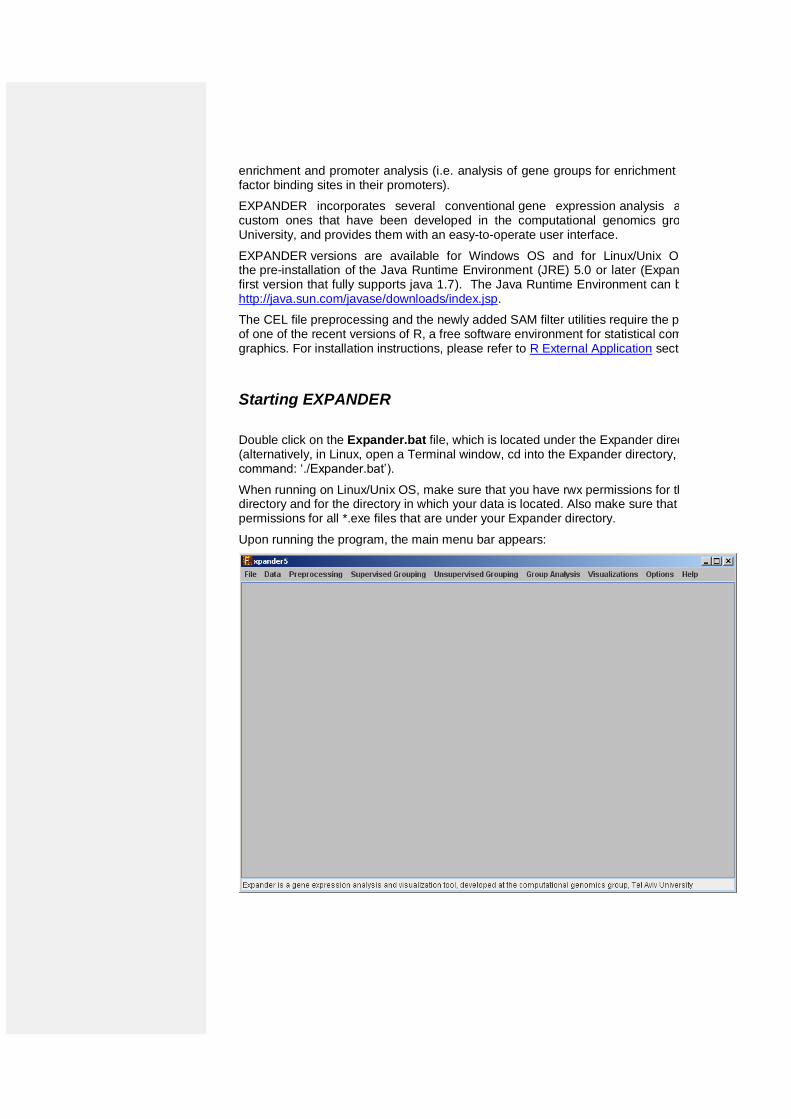
Upon running the program, the main menu bar appears:
Input Data
Expander operates on the following types of data:
a) Gene expression data – For most of EXPANDER's steps for analysis of gene expression data, the technique used for obtaining the expression estimates doesn't make a difference. Whatever technique (e.g., expression arrays, RNA-Seq) was used, the input expression data should be summarized in a matrix (tab-delimited txt file; see File Formats section) in which rows correspond to probes/genes and columns – to samples. Values can be either relative intensities data, expected as log 2 (R/G) values data (e.g. cDNA microarrays) OR absolute intensities data, expected as positive expression levels (E.g. High-density oligonucleotide data). Oligonucleotide data can be loaded with/without detection calls. Affymetrix data can also be loaded from CEL files (If R is installed).
When analyzing RNA-Seq data, one way to obtain gene expression matrix is to use TopHat (http://tophat.cbcb.umd.edu/tutorial.html ) to align the sequenced reads to the relevant genome, and then use Cufflinks (http://cufflinks.cbcb.umd.edu/howitworks.html ) or HTSeq (http://www-huber.embl.de/users/anders/HTSeq/doc/count.html#count ) to obtain gene (or transcript) expression estimates from TopHat output.
If one wishes to perform functional analysis or promoter analysis, an ID conversion file should be loaded along with the data file. The conversion file maps each probe ID (first column) in the data file into a corresponding conventional gene ID that is used in the GO annotation and TF fingerprint files that are supplied with EXPANDER. The conversion file can be loaded in the middle of the session too, by Data >> Load Conversion File.
b) Similarity data – a pre-calculated similarity matrix
c) Gene groups data – contains predefined groups of genes. In this data type, the conventional gene IDs that are used by EXPANDER in the GO annotation and TF fingerprint files are expected.
For details regarding the Gene ID convention that is used for each organism, refer to the Supplied Files section.
For details regarding the data files formats see the File Formats section.
Loading gene expression data:
Tabular Data File
To load tabular expression data, select: File >> New Session. From the submenu select Expression Data >> Tabular Data File.
When selecting Tabular Data File, the following dialog box will appear:
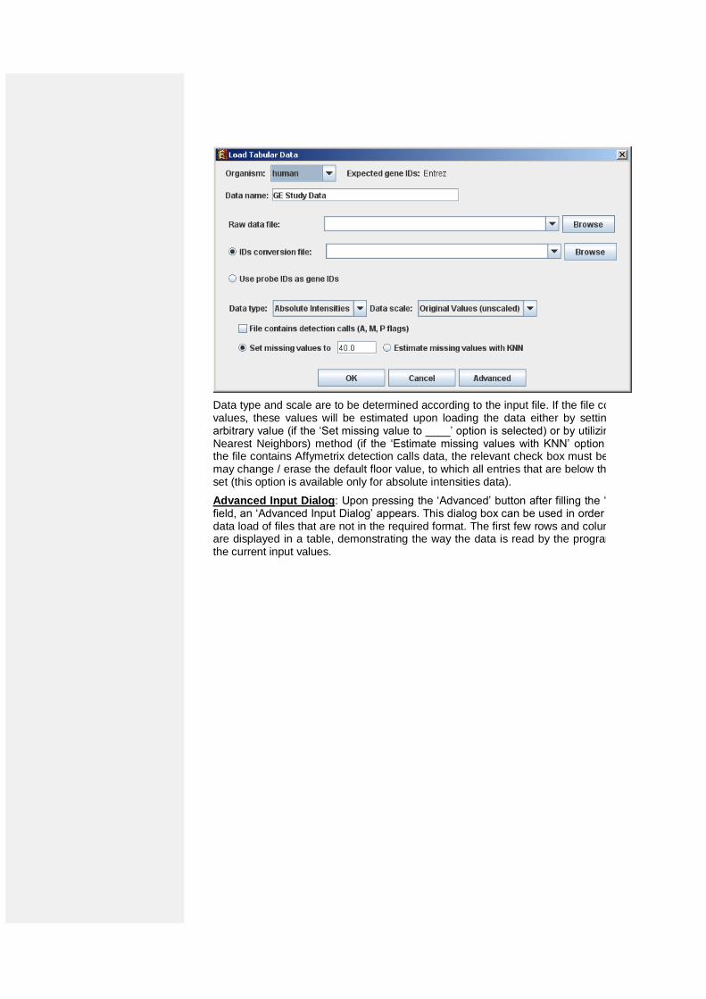
Data type and scale are to be determined according to the input file. If the file contains missing values, these values will be estimated upon loading the data either by setting them to and arbitrary value (if the ‘Set missing value to ____’ option is selected) or by utilizing the KNN (K-Nearest Neighbors) method (if the ‘Estimate missing values with KNN’ option is selected). If the file contains Affymetrix detection calls data, the relevant check box must be checked. You may change / erase the default floor value, to which all entries that are below that value will be set (this option is available only for absolute intensities data).
Advanced Input Dialog: Upon pressing the ‘Advanced’ button after filling the ‘Raw Data File’ field, an ‘Advanced Input Dialog’ appears. This dialog box can be used in order to facilitate the data load of files that are not in the required format. The first few rows and columns of the data are displayed in a table, demonstrating the way the data is read by the program according to the current input values.
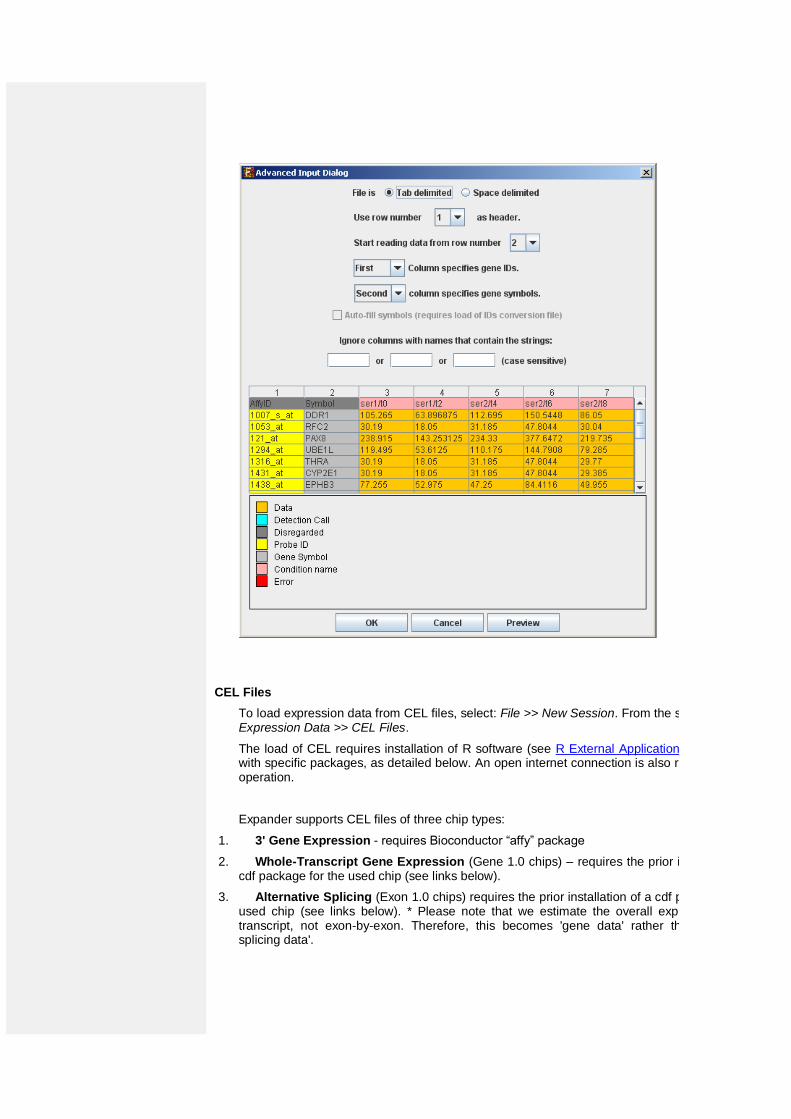
CEL Files
To load expression data from CEL files, select: File >> New Session. From the submenu select Expression Data >> CEL Files.
The load of CEL requires installation of R software (see R External Application section) along with specific packages, as detailed below. An open internet connection is also required for this operation.
Expander supports CEL files of three chip types:
1. 3' Gene Expression - requires Bioconductor “affy” package
2. Whole-Transcript Gene Expression (Gene 1.0 chips) – requires the prior installation of a cdf package for the used chip (see links below).
3. Alternative Splicing (Exon 1.0 chips) requires the prior installation of a cdf package for the used chip (see links below). * Please note that we estimate the overall expression for the transcript, not exon-by-exon. Therefore, this becomes 'gene data' rather than 'alternative splicing data'.
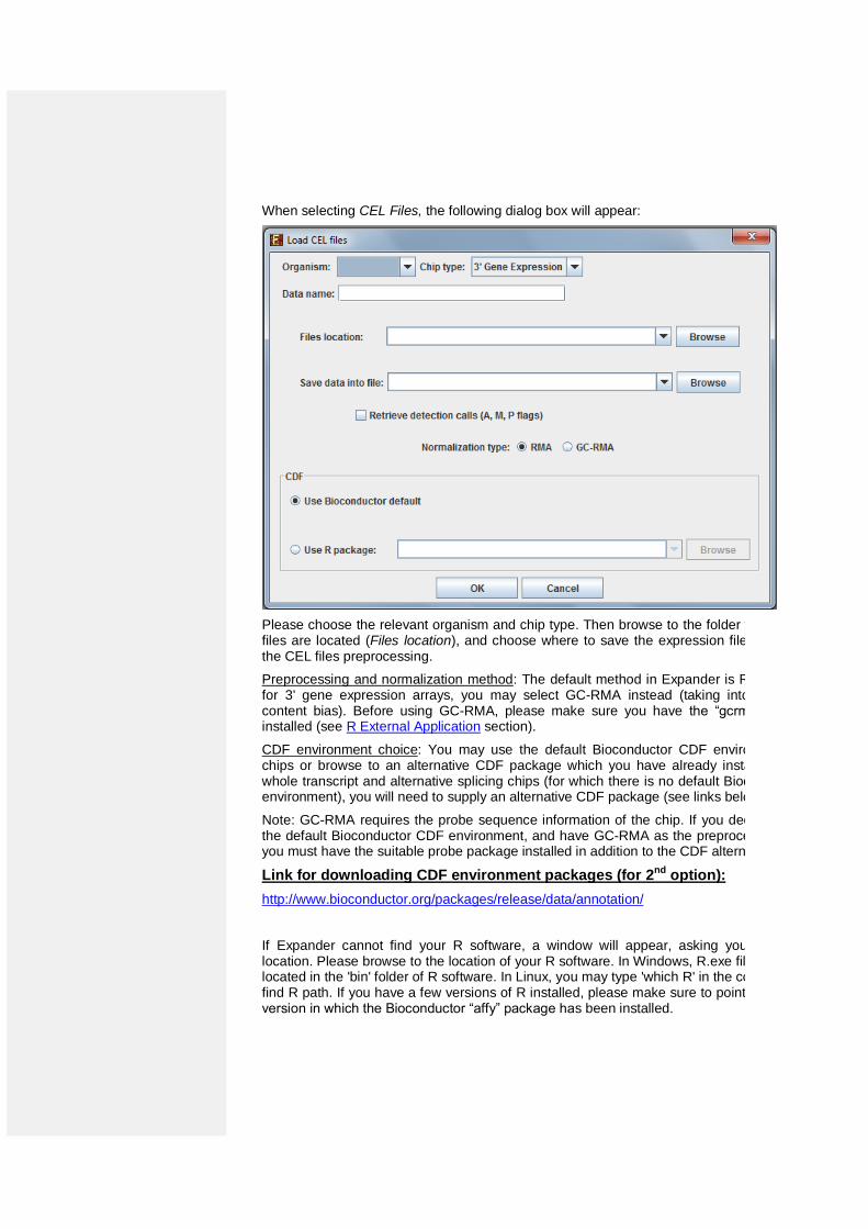
When selecting CEL Files, the following dialog box will appear:
Please choose the relevant organism and chip type. Then browse to the folder where the CEL files are located (Files location), and choose where to save the expression file resulting from the CEL files preprocessing.
Preprocessing and normalization method: The default method in Expander is RMA. However, for 3' gene expression arrays, you may select GC-RMA instead (taking into account GC-content bias). Before using GC-RMA, please make sure you have the “gcrma” R package installed (see R External Application section).
CDF environment choice: You may use the default Bioconductor CDF environment for the chips or browse to an alternative CDF package which you have already installed in R. For whole transcript and alternative splicing chips (for which there is no default Bioconductor CDF environment), you will need to supply an alternative CDF package (see links below).
Note: GC-RMA requires the probe sequence information of the chip. If you decide not to use the default Bioconductor CDF environment, and have GC-RMA as the preprocessing method, you must have the suitable probe package installed in addition to the CDF alternative package.
Link for downloading CDF environment packages (for 2nd option):
http://www.bioconductor.org/packages/release/data/annotation/
If Expander cannot find your R software, a window will appear, asking you to specify its location. Please browse to the location of your R software. In Windows, R.exe file is likely to be located in the 'bin' folder of R software. In Linux, you may type 'which R' in the command line to find R path. If you have a few versions of R installed, please make sure to point Expander to a version in which the Bioconductor “affy” package has been installed.
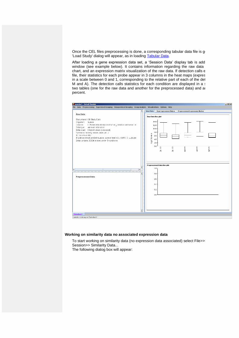
Once the CEL files preprocessing is done, a corresponding tabular data file is generated and a 'Load Study' dialog will appear, as in loading Tabular Data.
After loading a gene expression data set, a ‘Session Data’ display tab is added to the main window (see example below). It contains information regarding the raw data file, a box plot chart, and an expression matrix visualization of the raw data. If detection calls exist in the data file, their statistics for each probe appear in 3 columns in the heat maps (expression matrices), in a scale between 0 and 1, corresponding to the relative part of each of the detection calls (P, M and A). The detection calls statistics for each condition are displayed in a separate tab in two tables (one for the raw data and another for the preprocessed data) and are presented in percent.
Working on similarity data no associated expression data
To start working on similarity data (no expression data associated) select File>>New Session>> Similarity Data... The following dialog box will appear:
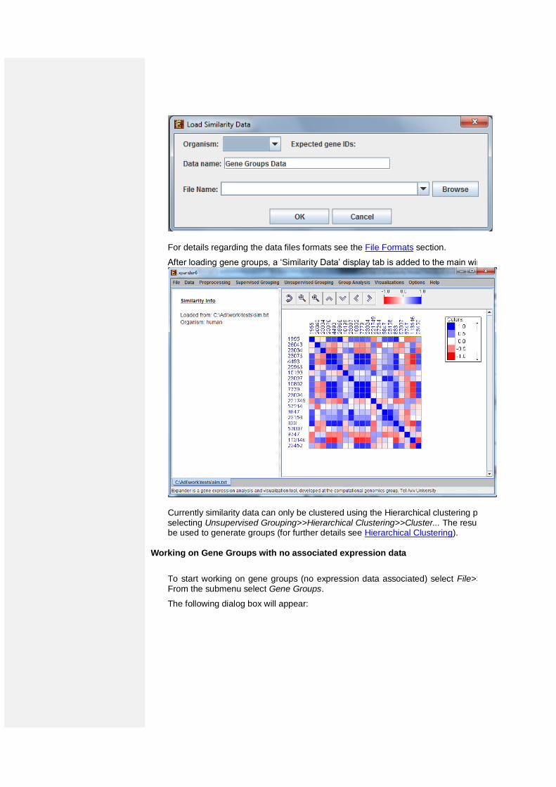
For details regarding the data files formats see the File Formats section.
After loading gene groups, a ‘Similarity Data’ display tab is added to the main window
Currently similarity data can only be clustered using the Hierarchical clustering procedure by selecting Unsupervised Grouping>>Hierarchical Clustering>>Cluster... The resulting tree can be used to generate groups (for further details see Hierarchical Clustering).
Working on Gene Groups with no associated expression data
To start working on gene groups (no expression data associated) select File>>New Session. From the submenu select Gene Groups.
The following dialog box will appear:
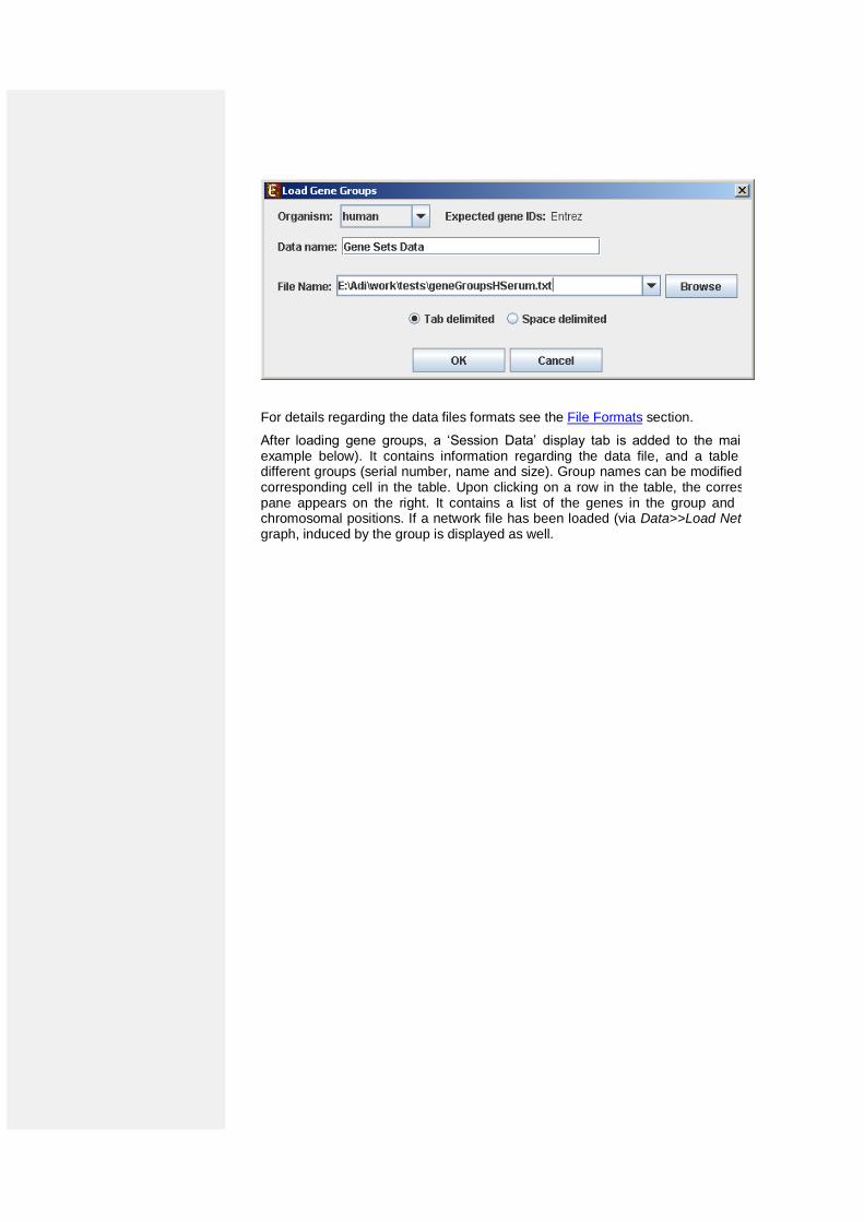
For details regarding the data files formats see the File Formats section.
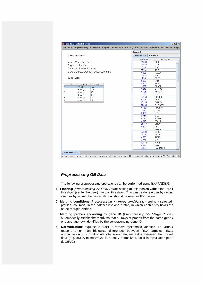
After loading gene groups, a ‘Session Data’ display tab is added to the main window (see example below). It contains information regarding the data file, and a table describing the different groups (serial number, name and size). Group names can be modified, by editing the corresponding cell in the table. Upon clicking on a row in the table, the corresponding group pane appears on the right. It contains a list of the genes in the group and a view of their chromosomal positions. If a network file has been loaded (via Data>>Load Network), the sub-graph, induced by the group is displayed as well.
Preprocessing GE Data
The following preprocessing operations can be performed using EXPANDER:
1) Flooring (Preprocessing >> Floor Data): setting all expression values that are bellow a certain threshold (set by the user) into that threshold. This can be done either by setting the floor value itself, or by setting the percentile that should be used as floor value.
2) Merging conditions (Preprocessing >> Merge conditions): merging a selected set of condition profiles (columns) in the dataset into one profile, in which each entry holds the average value of the merged entries.
3) Merging probes according to gene ID (Preprocessing >> Merge Probes by Gene ID): automatically shrinks the matrix so that all rows of probes from the same gene are merged into one average row, identified by the corresponding gene ID.
4) Normalization: required in order to remove systematic variation, i.e. variation arising from reasons other than biological differences between RNA samples. Expander performs normalization only for absolute intensities data, since it is assumed that the relative intensities data (e.g. cDNA microarrays) is already normalized, as it is input after performing log ratio (log2R/G).
Normalization can be performed using the following schemes:
a) Quantile normalization (Preprocessing >> Normalization >> Quantile), in which the whole data is used.
b) Non-linear baseline normalization (Preprocessing >> Normalization >> Non Linear Baseline), which uses a baseline array (can be selected by the user). In this scheme a normalization function is calculated using pseudo Loess regression of the M vs. A scatter plot. The subset of genes that are used to evaluate the normalization function can be set to ‘all genes’ (recommended when most genes in the dataset are expected to be constantly expressed) or a ‘rank invariant set’ of genes (recommended when there can be a large number of differentially expressed genes).
For more details regarding the normalization schemes see the References section.
5) Condition filtration: the conditions used in the analysis can be manually filtered by selecting: Preprocessing >> Filter Conditions. This will bring up a dialog box in which the user can select the required conditions from a list.
6) Gene (probe) filtration: can be performed in order to filter out some of the constantly expressed genes, and perform downstream analysis on a smaller informative subset of the genes.
Probe filtration can be performed using the following schemes:
a) t-Test (Preprocessing >> Filter Probes >> t-Test): When using this method, only probes that demonstrate differential expression between two condition subsets are selected.
b) SAM - Significance Analysis of Microarray (Preprocessing >> Filter Probes >> SAM):
selects probes that demonstrate differential expression between conditions subsets. You may choose 2 or more subsets (multi-class tests are supported). This method uses permutations to get an ’empirical’ estimate for the FDR of the reported differential genes (for details see the References section). Before using SAM, please make sure you have R software along with the “samr” package installed (see R External Application section).
c) Fold Change (Preprocessing >> Filter Probes >> Fold Change): when using this method only genes that are over/under expressed by at least n fold in at least k arrays are selected (n and k are determined by the user). The fold change can be calculated in relation to (a) a selected baseline array (b) the minimal expression value of the gene OR (c) the reference value when working on relative intensities (depending on the user’s selection).
d) Variation (Preprocessing >> Filter Probes >> Variation): In this method, the k most variant genes are selected (k is determined by the user). Variance is used to measure variation for relative intensities data, and Coefficient of Variation is used to measure variation for absolute intensities data.
e) Detection calls (Preprocessing >> Filter Probes >> Detection calls): in this method probes/genes are filtered according to the number of expression signals for which the detection call is ‘P’ (Present). It can only be operated if the data file contains detection info.
f) Load Probe Subset (Preprocessing >> Filter Probes >> Load Probe Subset): the filtered
set is loaded from an external txt file (for details regarding the format please see the File Formats section).
7) Divide by Base (Preprocessing >> Divide by Base) – Divides each entry in a profile (a column) by the corresponding entry in the profile of a selected base condition. This can be done for all conditions or for subsets of the conditions.
8) Log data (Preprocessing >> >> Log Data) – Performs log2 operation on each entry
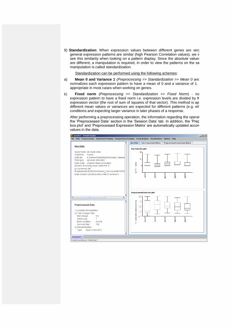
9) Standardization: When expression values between different genes are very different, but general expression patterns are similar (high Pearson Correlation values), we would expect to see this similarity when looking on a pattern display. Since the absolute values of expression are different, a manipulation is required, in order to view the patterns on the same scale. This manipulation is called standardization.
Standardization can be performed using the following schemes:
a) Mean 0 and Variance 1 (Preprocessing >> Standardization >> Mean 0 and Variance 1) – normalizes each expression pattern to have a mean of 0 and a variance of 1. This method is appropriate in most cases when working on genes.
b) Fixed norm (Preprocessing >> Standardization >> Fixed Norm) - normalizes each expression pattern to have a fixed norm i.e. expression levels are divided by the norm of that expression vector (the root of sum of squares of that vector). This method is appropriate when different mean values or variances are expected for different patterns (e.g. when working on conditions and expecting larger variance in later phases of a response.
After performing a preprocessing operation, the information regarding the operation is added to the ‘Preprocessed Data’ section in the ‘Session Data’ tab. In addition, the ‘Preprocessed Data box plot’ and ‘Preprocessed Expression Matrix’ are automatically updated according to the new values in the data.
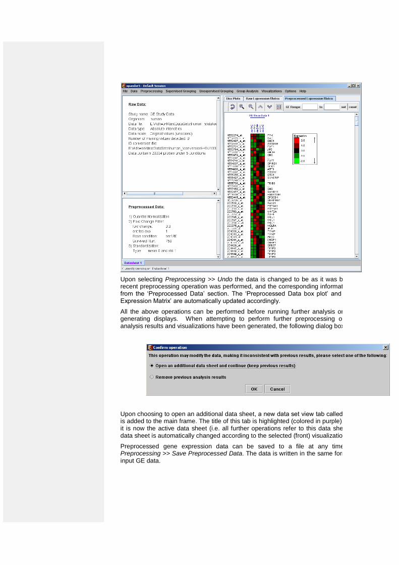
Upon selecting Preprocessing >> Undo the data is changed to be as it was before the most recent preprocessing operation was performed, and the corresponding information is removed from the ‘Preprocessed Data’ section. The ‘Preprocessed Data box plot’ and ‘Preprocessed Expression Matrix’ are automatically updated accordingly.
All the above operations can be performed before running further analysis on the data and generating displays. When attempting to perform further preprocessing operations after analysis results and visualizations have been generated, the following dialog box appears:
Upon choosing to open an additional data sheet, a new data set view tab called ‘Data Sheet 2’ is added to the main frame. The title of this tab is highlighted (colored in purple), indicating that it is now the active data sheet (i.e. all further operations refer to this data sheet). The active data sheet is automatically changed according to the selected (front) visualization tab.
Preprocessed gene expression data can be saved to a file at any time be selecting Preprocessing >> Save Preprocessed Data. The data is written in the same format defined for input GE data.
Viewing Data Plots
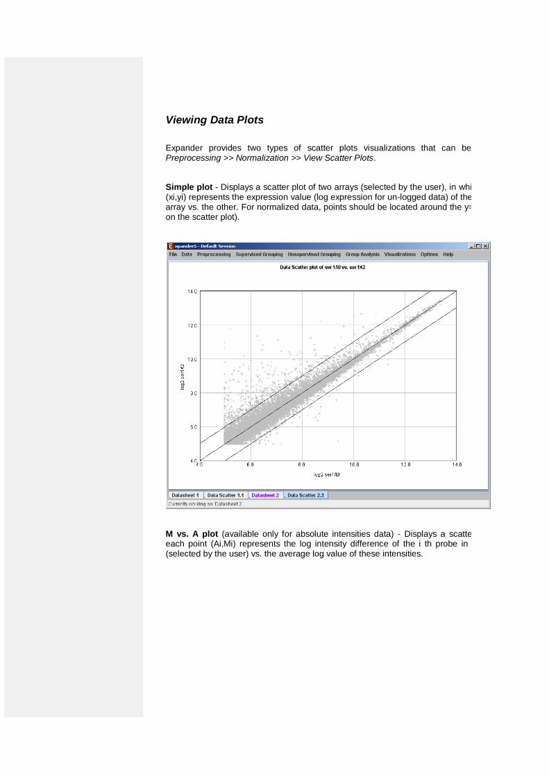
Expander provides two types of scatter plots visualizations that can be operated via Preprocessing >> Normalization >> View Scatter Plots.
Simple plot - Displays a scatter plot of two arrays (selected by the user), in which the ith point (xi,yi) represents the expression value (log expression for un-logged data) of the ith gene in one array vs. the other. For normalized data, points should be located around the y=x line (marked on the scatter plot).
M vs. A plot (available only for absolute intensities data) - Displays a scatter plot in which each point (Ai,Mi) represents the log intensity difference of the i th probe in the two arrays (selected by the user) vs. the average log value of these intensities.
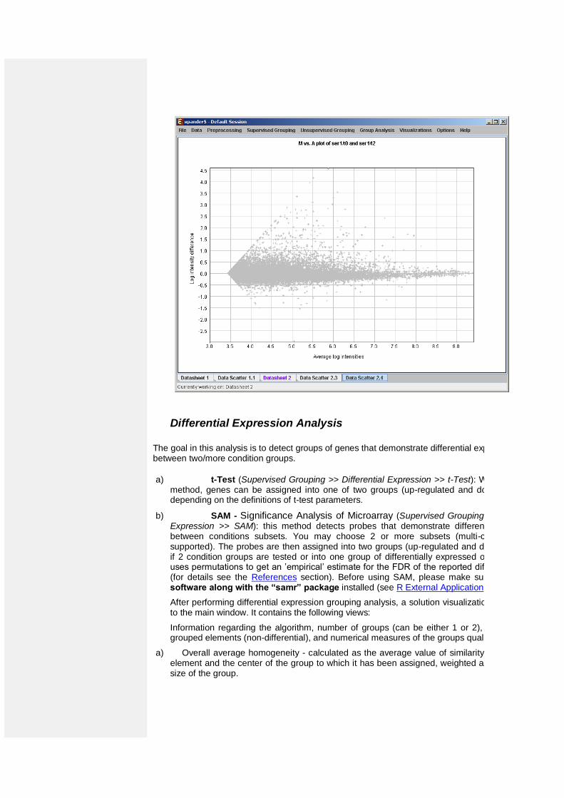
Differential Expression Analysis
The goal in this analysis is to detect groups of genes that demonstrate differential expression between two/more condition groups.
a) t-Test (Supervised Grouping >> Differential Expression >> t-Test): When using this
method, genes can be assigned into one of two groups (up-regulated and down-regulated), depending on the definitions of t-test parameters.
b) SAM - Significance Analysis of Microarray (Supervised Grouping >> Differential Expression >> SAM): this method detects probes that demonstrate differential expression between conditions subsets. You may choose 2 or more subsets (multi-class tests are supported). The probes are then assigned into two groups (up-regulated and down-regulated) if 2 condition groups are tested or into one group of differentially expressed otherwise. SAM uses permutations to get an ’empirical’ estimate for the FDR of the reported differential genes (for details see the References section). Before using SAM, please make sure you have R software along with the “samr” package installed (see R External Application section).
After performing differential expression grouping analysis, a solution visualization tab is added to the main window. It contains the following views:
Information regarding the algorithm, number of groups (can be either 1 or 2), number of un-grouped elements (non-differential), and numerical measures of the groups quality, including:
a) Overall average homogeneity - calculated as the average value of similarity between each element and the center of the group to which it has been assigned, weighted according to the size of the group.
b) Overall average separation – calculated as the average similarity between mean patterns of different groups, weighted according to their sizes.
c) Groups table - contains the number, name (label), size and homogeneity of each group.
Mean Patterns of the groups with error bars (±1 STD).
Upon selecting a group, the corresponding pane is displayed on the right. It contains a list of probes, p-values/q-values, fold-change, probe patterns, expression matrix (heat map) and the chromosomal locations of the genes. Similarity matrices for probes within the cluster as well as for conditions are also displayed in this tab, if the relevant options in the display settings are selected (see the Settings section). If a network file has been loaded (via Data>>Load Network), the sub-graph, induced by the cluster is also displayed in the group pane.
In order to allow comparison between groups and patterns, the displayed expression patterns are automatically standardized to have mean = 0 and STD = 1.
A differential expression solution can be saved using the Supervised Grouping >> Differential Expression >> Save Solution, and reloaded using the Grouping Supervised Grouping >> Differential Expression >> Load Solution.
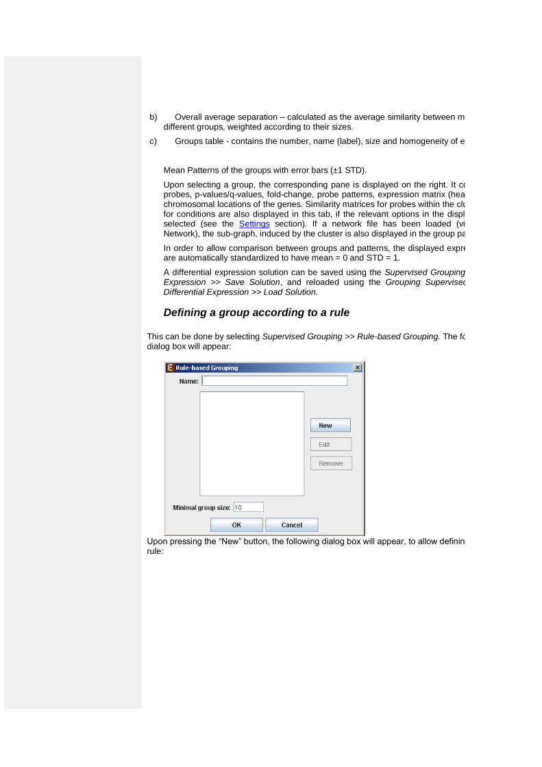
Defining a group according to a rule
This can be done by selecting Supervised Grouping >> Rule-based Grouping. The following input dialog box will appear:
Upon pressing the “New” button, the following dialog box will appear, to allow defining the group rule:
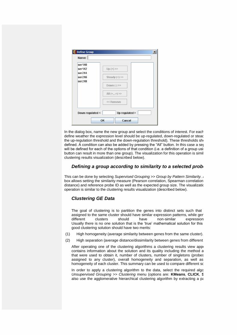
In the dialog box, name the new group and select the conditions of interest. For each condition define weather the expression level should be up-regulated, down-regulated or steady (between the up-regulation threshold and the down-regulation threshold). These thresholds should also be defined. A condition can also be added by pressing the “All” button. In this case a separate group will be defined for each of the options of that condition (i.e. a definition of a group using the “All” button can result in more than one group). The visualization for this operation is similar to the clustering results visualization (described below).
Defining a group according to similarity to a selected probe This can be done by selecting Supervised Grouping >> Group by Pattern Similarity. An input dialog box allows setting the similarity measure (Pearson correlation, Spearman correlation or Euclidean distance) and reference probe ID as well as the expected group size. The visualization for this operation is similar to the clustering results visualization (described below).
Clustering GE Data
The goal of clustering is to partition the genes into distinct sets such that genes that are assigned to the same cluster should have similar expression patterns, while genes assigned to different clusters should have non-similar expression patterns. Usually there is no one solution that is the ‘true’ mathematical solution for this problem, but a good clustering solution should have two merits:
(1) High homogeneity (average similarity between genes from the same cluster).
(2) High separation (average distance/dissimilarity between genes from different clusters).
After operating one of the clustering algorithms a clustering results view appears. The view contains information about the solution and its quality including the method and parameters that were used to obtain it, number of clusters, number of singletons (probes that were not assigned to any cluster), overall homogeneity and separation, as well as the size and homogeneity of each cluster. This summary can be used to compare different solutions.
In order to apply a clustering algorithm to the data, select the required algorithm from the Unsupervised Grouping >> Clustering menu (options are: KMeans, CLICK, SOM). You can also use the agglomerative hierarchical clustering algorithm by extracting a partition from an
existing hierarchical tree, by selecting Unsupervised Grouping >> Hierarchical Clustering>> Generate Groups (For details about building such a tree, please go to Hierarchical Clustering).
Currently similarity data can only be clustered using the Hierarchical clustering procedure by selecting Unsupervised Grouping>>Hierarchical Clustering>>Cluster... The resulting tree can be used to generate groups (for further details see Hierarchical Clustering).
An existing clustering solution can be loaded from a file by selecting Unsupervised Grouping >> Clustering >>Load Solution (For details regarding the clustering solution file format, refer to the File Formats section). The CLICK algorithm is not designed to find clusters under the size of 15 probes, so it might fail in clustering small datasets.
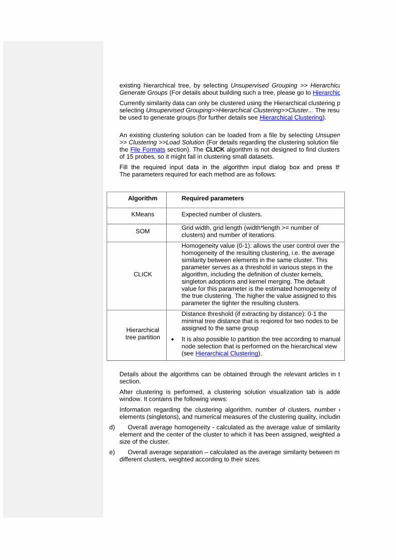
Fill the required input data in the algorithm input dialog box and press the ‘Ok’ button. The parameters required for each method are as follows:
Details about the algorithms can be obtained through the relevant articles in the References section.
After clustering is performed, a clustering solution visualization tab is added to the main window. It contains the following views:
Information regarding the clustering algorithm, number of clusters, number of un-clustered elements (singletons), and numerical measures of the clustering quality, including:
d) Overall average homogeneity - calculated as the average value of similarity between each element and the center of the cluster to which it has been assigned, weighted according to the size of the cluster.
e) Overall average separation – calculated as the average similarity between mean patterns of different clusters, weighted according to their sizes.
Algorithm Required parameters
KMeans Expected number of clusters.
SOM Grid width, grid length (width*length >= number of clusters) and number of iterations.
CLICK
Homogeneity value (0-1): allows the user control over the homogeneity of the resulting clustering, i.e. the average similarity between elements in the same cluster. This parameter serves as a threshold in various steps in the algorithm, including the definition of cluster kernels, singleton adoptions and kernel merging. The default value for this parameter is the estimated homogeneity of the true clustering. The higher the value assigned to this parameter the tighter the resulting clusters.
Hierarchical tree partition
Distance threshold (if extracting by distance): 0-1 the minimal tree distance that is reqiored for two nodes to be assigned to the same group
It is also possible to partition the tree according to manual node selection that is performed on the hierarchical view (see Hierarchical Clustering).
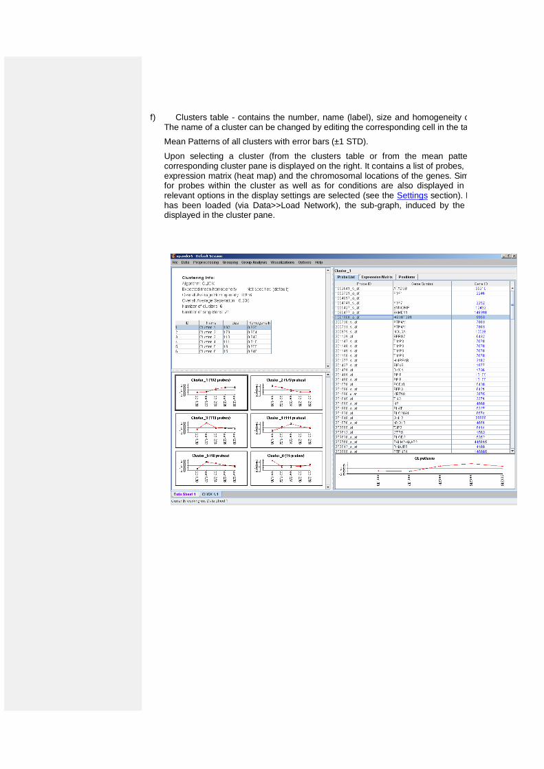
f) Clusters table - contains the number, name (label), size and homogeneity of each cluster. The name of a cluster can be changed by editing the corresponding cell in the table.
Mean Patterns of all clusters with error bars (±1 STD).
Upon selecting a cluster (from the clusters table or from the mean patterns view), the corresponding cluster pane is displayed on the right. It contains a list of probes, probe patterns, expression matrix (heat map) and the chromosomal locations of the genes. Similarity matrices for probes within the cluster as well as for conditions are also displayed in this tab, if the relevant options in the display settings are selected (see the Settings section). If a network file has been loaded (via Data>>Load Network), the sub-graph, induced by the cluster is also displayed in the cluster pane.
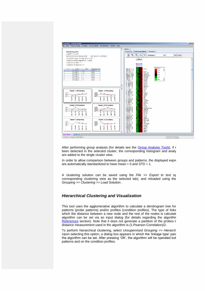
After performing group analysis (for details see the Group Analysis Tools), if enrichment has been detected in the selected cluster, the corresponding histogram and analysis information are added to the single cluster view.
In order to allow comparison between groups and patterns, the displayed expression patterns are automatically standardized to have mean = 0 and STD = 1.
A clustering solution can be saved using the File >> Export to text option (with the corresponding clustering view as the selected tab), and reloaded using the Unsupervised Grouping >> Clustering >> Load Solution.
Hierarchical Clustering and Visualization
This tool uses the agglomerative algorithm to calculate a dendrogram tree for all expression patterns (probe patterns) and/or profiles (condition profiles). The type of linkage (manner in which the distance between a new node and the rest of the nodes is calculated) used in the algorithm can be set via an input dialog (for details regarding the algorithms refer to the References section). Note that it does not generate a partition of the probes to clusters. The distance measurement used in the algorithm is (1-Pearson Correlation)/2.
To perform hierarchical clustering, select Unsupervised Grouping >> Hierarchical Clustering. Upon selecting this option, a dialog box appears in which the ‘linkage type’ parameter, used in the algorithm can be set. After pressing ‘OK’, the algorithm will be operated both on the probe patterns and on the condition profiles.
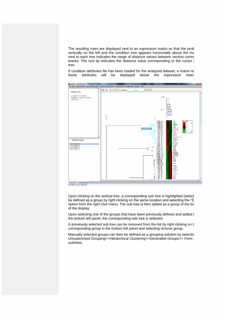
The resulting trees are displayed next to an expression matrix so that the probe tree appears vertically on the left and the condition tree appears horizontally above the matrix. The scale next to each tree indicates the range of distance values between vectors corresponding to the leaves. The tool tip indicates the distance value corresponding to the cursor location on the tree.
If condition attributes file has been loaded for the analyzed dataset, a matrix representation of these attributes will be displayed below the expression matrix (heatmap).
Upon clicking on the vertical tree, a corresponding sub tree is highlighted (selected) and can be defined as a group by right clicking on the same location and selecting the “Export group” option from the right click menu. The sub tree is then added as a group of the bottom left panel of the display.
Upon selecting one of the groups that have been previously defined and added to the list on the bottom left panel, the corresponding sub tree is selected.
A previously selected sub tree can be removed from the list by right clicking on the corresponding group in the bottom left panel and selecting remove group.
Manually selected groups can then be defined as a grouping solution by selecting Unsupervised Grouping>>Hierarchical Clustering>>Generated Groups>> From Selected subtrees.
Biclustering GE Data
Biclustering is clustering of both genes and conditions of the data into subgroups that are not necessarily disjoint. It enables the user to detect genes that are co-regulated in only a subgroup of the conditions, and does not force genes to belong exclusively to one cluster. It is useful when working on datasets which contain a large number of conditions.
Expander incorporates two Biclustering algorithms: ISA (Iterative Signature Algorithm) and SAMBA algorithm (for details see the References section). Before using ISA, please make sure you have R software along with the “eisa” package installed (see R External Application section).
In order to apply the ISA algorithm to the data select Grouping>>Bi-Clustering>>ISA. This operation does not require parameter input.
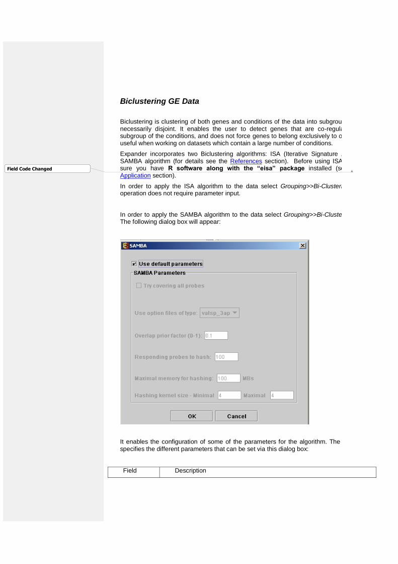
In order to apply the SAMBA algorithm to the data select Grouping>>Bi-Clustering>>SAMBA. The following dialog box will appear:
It enables the configuration of some of the parameters for the algorithm. The following table specifies the different parameters that can be set via this dialog box:
Field Description
Field Code Changed
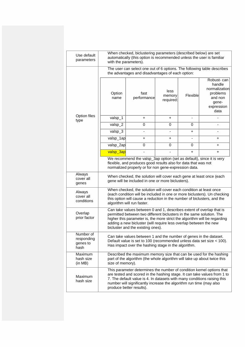
Use default parameters
When checked, biclustering parameters (described below) are set automatically (this option is recommended unless the user is familiar with the parameters).
Option files type
The user can select one out of 6 options. The following table describes the advantages and disadvantages of each option:
Robust- can handle
normalization problems and non gene-
expression data
Flexible less
memory required:
fast performance
Option name
- - + + valsp_1
- 0 0 0 valsp_2
- + - - valsp_3
+ - + + valsp_1ap
+ 0 0 0 valsp_2ap
+ + - - valsp_3ap
We recommend the valsp_3ap option (set as default), since it is very flexible, and produces good results also for data that was not normalized properly or for non gene-expression data.
Always cover all genes
When checked, the solution will cover each gene at least once (each gene will be included in one or more biclusters).
Always cover all conditions
When checked, the solution will cover each condition at least once (each condition will be included in one or more biclusters). Un checking this option will cause a reduction in the number of biclusters, and the algorithm will run faster.
Overlap prior factor
Can take values between 0 and 1, describes extent of overlap that is permitted between two different biclusters in the same solution. The higher this parameter is, the more strict the algorithm will be regarding adding a new bicluster (will require less overlap between the new bicluster and the existing ones).
Number of responding genes to hash
Can take values between 1 and the number of genes in the dataset. Default value is set to 100 (recommended unless data set size < 100). Has impact over the hashing stage in the algorithm.
Maximum hash size (in MB)
Described the maximum memory size that can be used for the hashing part of the algorithm (the whole algorithm will take up about twice this size of memory).
Maximum hash size
This parameter determines the number of condition kernel options that are tested and scored in the hashing stage. It can take values from 1 to 7. The default value is 4. In datasets with many conditions raising this number will significantly increase the algorithm run time (may also produce better results).
Minimum hash size
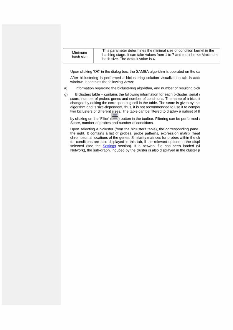
This parameter determines the minimal size of condition kernel in the hashing stage. It can take values from 1 to 7 and must be <= Maximum hash size. The default value is 4.
Upon clicking ‘OK’ in the dialog box, the SAMBA algorithm is operated on the dataset.
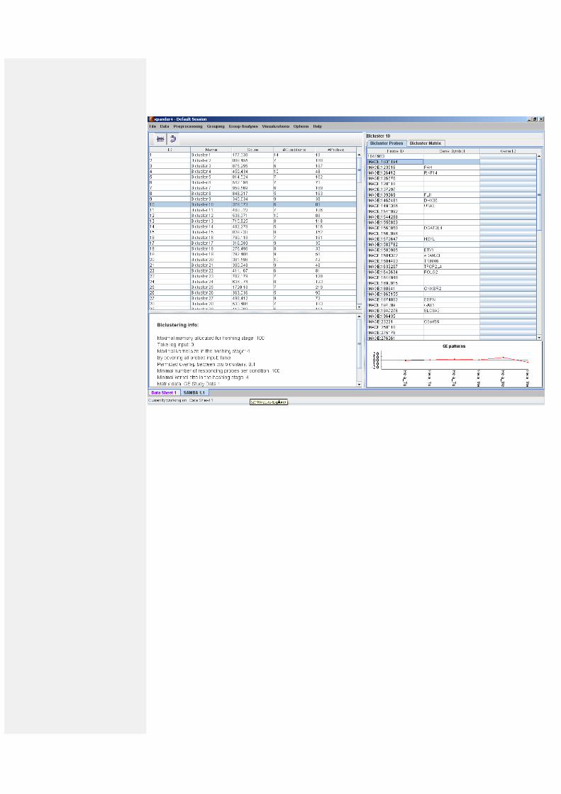
After biclustering is performed a biclustering solution visualization tab is added to the main window. It contains the following views:
a) Information regarding the biclustering algorithm, and number of resulting biclusters.
g) Biclusters table – contains the following information for each bicluster: serial number, name, score, number of probes genes and number of conditions. The name of a bicluster can be changed by editing the corresponding cell in the table. The score is given by the SAMBA algorithm and is size-dependent, thus, it is not recommended to use it to compare the quality of two biclusters of different sizes. The table can be filtered to display a subset of the biclusters
by clicking on the ‘Filter’ ( ) button in the toolbar. Filtering can be performed according to: Score, number of probes and number of conditions.
Upon selecting a bicluster (from the biclusters table), the corresponding pane is displayed on the right. It contains a list of probes, probe patterns, expression matrix (heat map) and the chromosomal locations of the genes. Similarity matrices for probes within the cluster as well as for conditions are also displayed in this tab, if the relevant options in the display settings are selected (see the Settings section). If a network file has been loaded (via Data>>Load Network), the sub-graph, induced by the cluster is also displayed in the cluster pane.
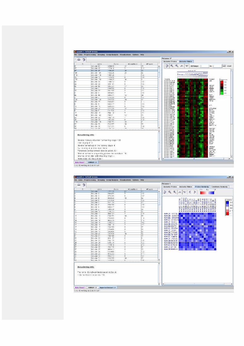
After performing group analysis (for details see the Group Analysis Tools section), if enrichment has been detected in the selected bicluster, the corresponding histogram and analysis information are added to the single bicluster view, and a column is added to the expression matrix display for each enrichment class, stating for each probe, whether it belongs to that class.
A biclustering solution can be saved using the Grouping >> Bi-Clustering >> Save Solution, and reloaded using the Grouping >> Bi-Clustering >> Load Solution. For a format of the solution file, please refer to the File Formats section:
Network Based Grouping of GE Data
The goal here is to detect groups of genes that demonstrate similar expression patterns and are also highly connected in a given interactions network.
In order to operate these tools, an interactions network in .SIF format needs to be loaded. This can be done either by selecting Data>>Load network or via the dialog boxes of the tools.
In order to perform network based grouping Expander incorporates two algorithms: Matisse and Degas (for details see the References section). The DEGAS algorithm is relevant when the expression dataset compares two groups of heterogeneous samples (as in case-control studies). The groups detected by these tools are referred to as “modules” and may contain also genes that exist in the network, but are not present in the filtered GE data (referred to as “Back nodes”).
To use the more advanced, stand-alone versions of MATISSE and DEGAS (with higher flexibility), please refer to the Matisse home page.
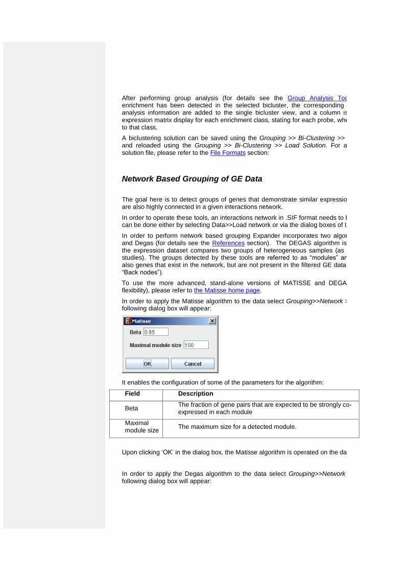
In order to apply the Matisse algorithm to the data select Grouping>>Network >>Matisse. The following dialog box will appear:
It enables the configuration of some of the parameters for the algorithm:
Field Description
Beta The fraction of gene pairs that are expected to be strongly co-expressed in each module
Maximal module size
The maximum size for a detected module.
Upon clicking ‘OK’ in the dialog box, the Matisse algorithm is operated on the dataset.
In order to apply the Degas algorithm to the data select Grouping>>Network >>Degas. The following dialog box will appear:
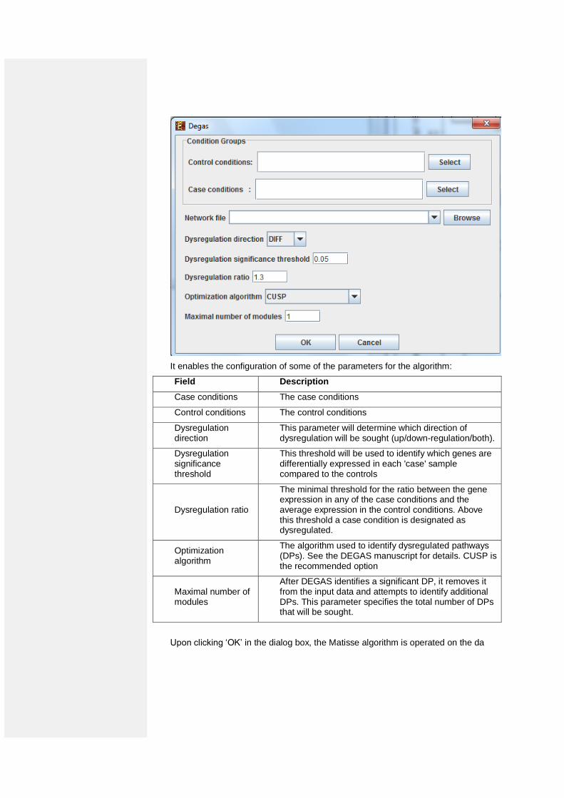
It enables the configuration of some of the parameters for the algorithm:
Field Description
Case conditions The case conditions
Control conditions The control conditions
Dysregulation direction
This parameter will determine which direction of dysregulation will be sought (up/down-regulation/both).
Dysregulation significance threshold
This threshold will be used to identify which genes are differentially expressed in each 'case' sample compared to the controls
Dysregulation ratio
The minimal threshold for the ratio between the gene expression in any of the case conditions and the average expression in the control conditions. Above this threshold a case condition is designated as dysregulated.
Optimization algorithm
The algorithm used to identify dysregulated pathways (DPs). See the DEGAS manuscript for details. CUSP is the recommended option
Maximal number of modules
After DEGAS identifies a significant DP, it removes it from the input data and attempts to identify additional DPs. This parameter specifies the total number of DPs that will be sought.
Upon clicking ‘OK’ in the dialog box, the Matisse algorithm is operated on the dataset.
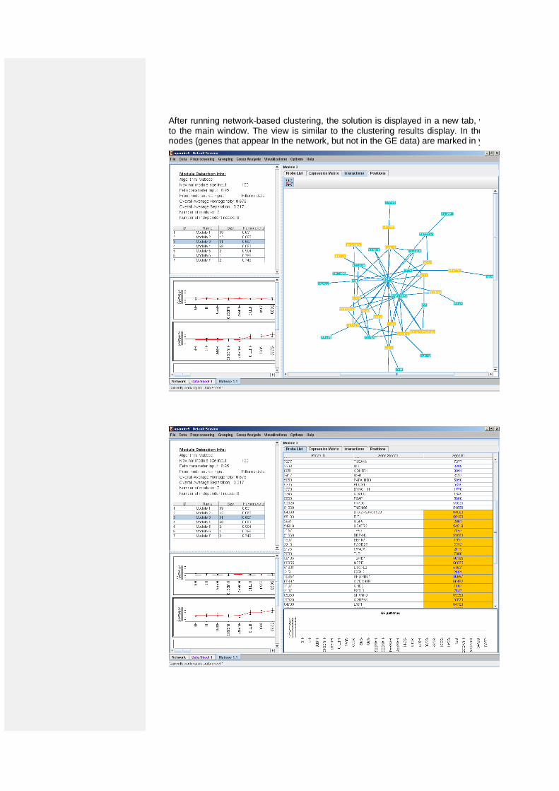
After running network-based clustering, the solution is displayed in a new tab, which is added to the main window. The view is similar to the clustering results display. In the display, back nodes (genes that appear In the network, but not in the GE data) are marked in yellow.
After performing group analysis (for details see the Group Analysis Tools section), if enrichment has been detected in the selected module, the corresponding histogram and analysis information are added to the single module view, and a column is added to the expression matrix display for each enrichment class, stating for each probe, whether it belongs to that class.
A network-based grouping solution can be saved using the Grouping >> Network >> Save Solution, and reloaded using the Grouping >> Network >> Load Solution. For a format of the solution file, please refer to the File Formats section:
Group Enrichments Analysis Tools
The following analysis can be performed on gene sets, clusters, biclusters, network based modules, similarity based groups, or the filtered dataset (the analyzed set of probes as one set). Before operating any of the group analysis operation (not including the “General enrichment analysis”), the data files for the relevant organism should be downloaded. The files for a specific organism are supplied as one single zip file that you need to download from the Expander download page, section "Organism specific data" (can be reached from inside Expander: Help >> Open download page, or from updates.html file in your Expander directory). Then, you extract the file into "Expander/organisms" directory. The relevant directories will be built by the extraction, inside your "Expander/organisms" directory. For example, after extracting human data, you should have "Expander/organisms/human" directory.
Functional Analysis
This tool performs basic statistical analysis on the distribution of functions of genes within each cluster. The functions of the genes are determined according to annotation files (GO), which can be downloaded from the EXPANDER download page (see the Supplied Files section). To perform this analysis, Expander utilizes the TANGO software, which performs hyper-geometric enrichment tests and corrects for multiple testing by bootstrapping and estimating the empirical p-value distribution for the evaluated sets.
Before operating functional analysis the annotation files for the relevant organism should be
downloaded from the download page (more details at introduction of Group_Analysis Tools).
To perform the analysis, select Group Analysis >> Functional Analysis >> TANGO. The following dialog box will appear:
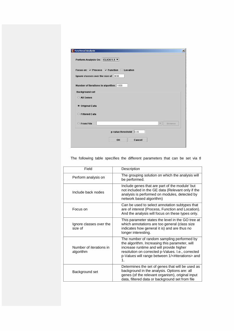
The following table specifies the different parameters that can be set via this dialog box:
Field Description
Perform analysis on The grouping solution on which the analysis will be performed.
Include back nodes
Include genes that are part of the module' but not included in the GE data (Relevant only if the analysis is performed on modules, detected by network based algorithm)
Focus on Can be used to select annotation subtypes that are of interest (Process, Function and Location). And the analysis will focus on these types only.
Ignore classes over the size of
This parameter states the level in the GO tree at which annotations are too general (class size indicates how general it is) and are thus no longer interesting.
Number of iterations in algorithm
The number of random sampling performed by the algorithm. Increasing this parameter, will increase runtime and will provide higher resolution on corrected p-Values. I.e., corrected p-Values will range between 1/<#iterations> and 1.
Background set
Determines the set of genes that will be used as background in the analysis. Options are: all genes (of the relevant organism), original input data, filtered data or background set from file
(see the Files Format section for details regarding the format of an external background set).
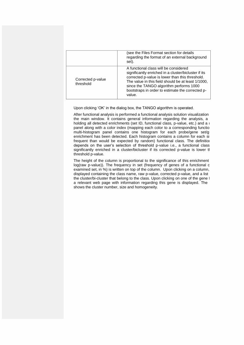
Corrected p-value threshold
A functional class will be considered significantly enriched in a cluster/bicluster if its corrected p-value is lower than this threshold. The value in this field should be at least 1/1000, since the TANGO algorithm performs 1000 bootstraps in order to estimate the corrected p-value.
Upon clicking ‘OK’ in the dialog box, the TANGO algorithm is operated.
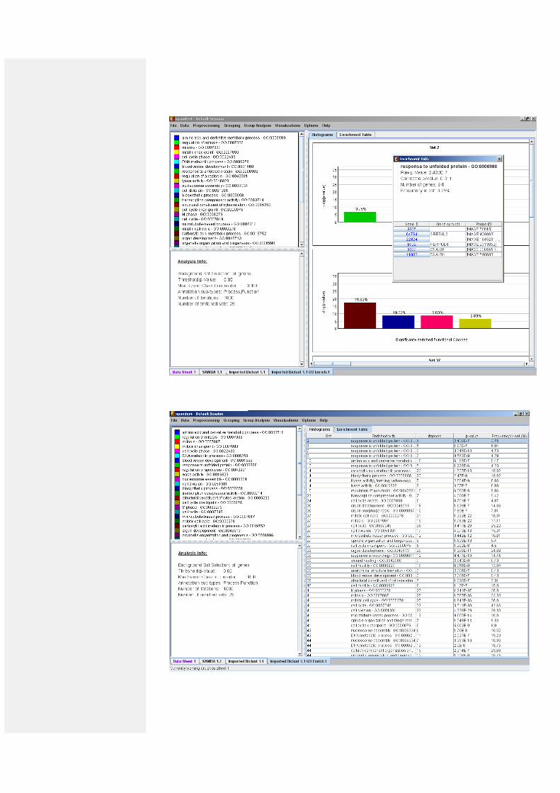
After functional analysis is performed a functional analysis solution visualization tab is added to the main window. It contains general information regarding the analysis, a sort-able table holding all detected enrichments (set ID, functional class, p-value, etc.) and a multi-histogram panel along with a color index (mapping each color to a corresponding functional class). The multi-histogram panel contains one histogram for each probe/gene set/group in which enrichment has been detected. Each histogram contains a column for each significant (more frequent than would be expected by random) functional class. The definition of significant depends on the user’s selection of threshold p-value i.e., a functional class is considered significantly enriched in a cluster/bicluster if its corrected p-value is lower than the preset threshold p-value.
The height of the column is proportional to the significance of this enrichment (i.e. height = -log(raw p-value)). The frequency in set (frequency of genes of a functional class within the examined set, in %) is written on top of the column. Upon clicking on a column, a dialog box is displayed containing the class name, raw p-value, corrected p-value, and a list of the genes in the cluster/bi-cluster that belong to the class. Upon clicking on one of the gene Ids in the table, a relevant web page with information regarding this gene is displayed. The display tool tip shows the cluster number, size and homogeneity.
Annotation files are currently supplied with EXPANDER for yeast, human, mouse, rat, fly, zebrafish, c-elegans, Arabidopsis, chicken and E. coli, and are updated on a regular basis (for more information, refer to the Supplied Files section).
The results of this analysis can be exported to a text file by selecting File>>Export to text when the corresponding view is the selected tab.
Promoter Analysis
PRIMA
This tool identifies TFs whose binding sites are significantly over-represented in a given set of promoters (i.e. cluster or bicluster). To perform this analysis Expander utilizes the PRIMA (PRomoter Integration in Microarray Analysis) software which performs a statistical analysis on the distribution of transcription factor motifs in the promoters of genes within each cluster or bicluster. To achieve this, PRIMA uses preprocessed TF fingerprint files, which can be downloaded from the EXPANDER download-page (see the Supplied Files section), and are updated on a regular basis. For details regarding the PRIMA software see the References section.
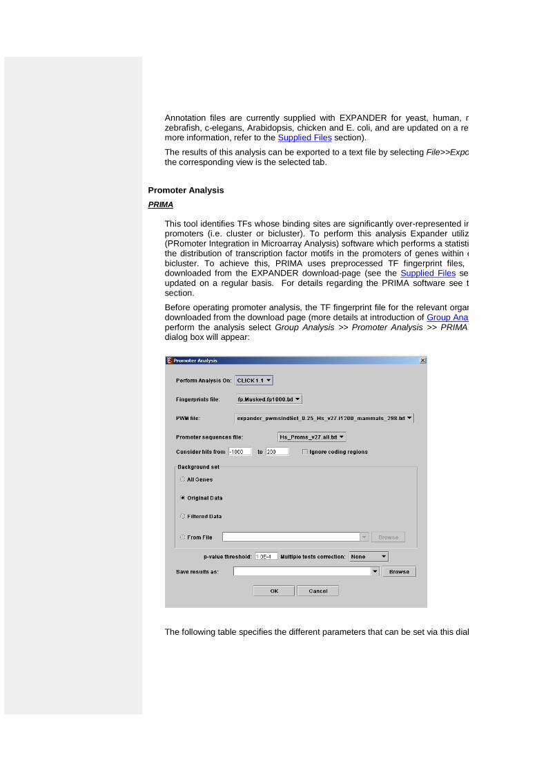
Before operating promoter analysis, the TF fingerprint file for the relevant organism should be downloaded from the download page (more details at introduction of Group Analysis Tools). To perform the analysis select Group Analysis >> Promoter Analysis >> PRIMA. The following dialog box will appear:
The following table specifies the different parameters that can be set via this dialog box:
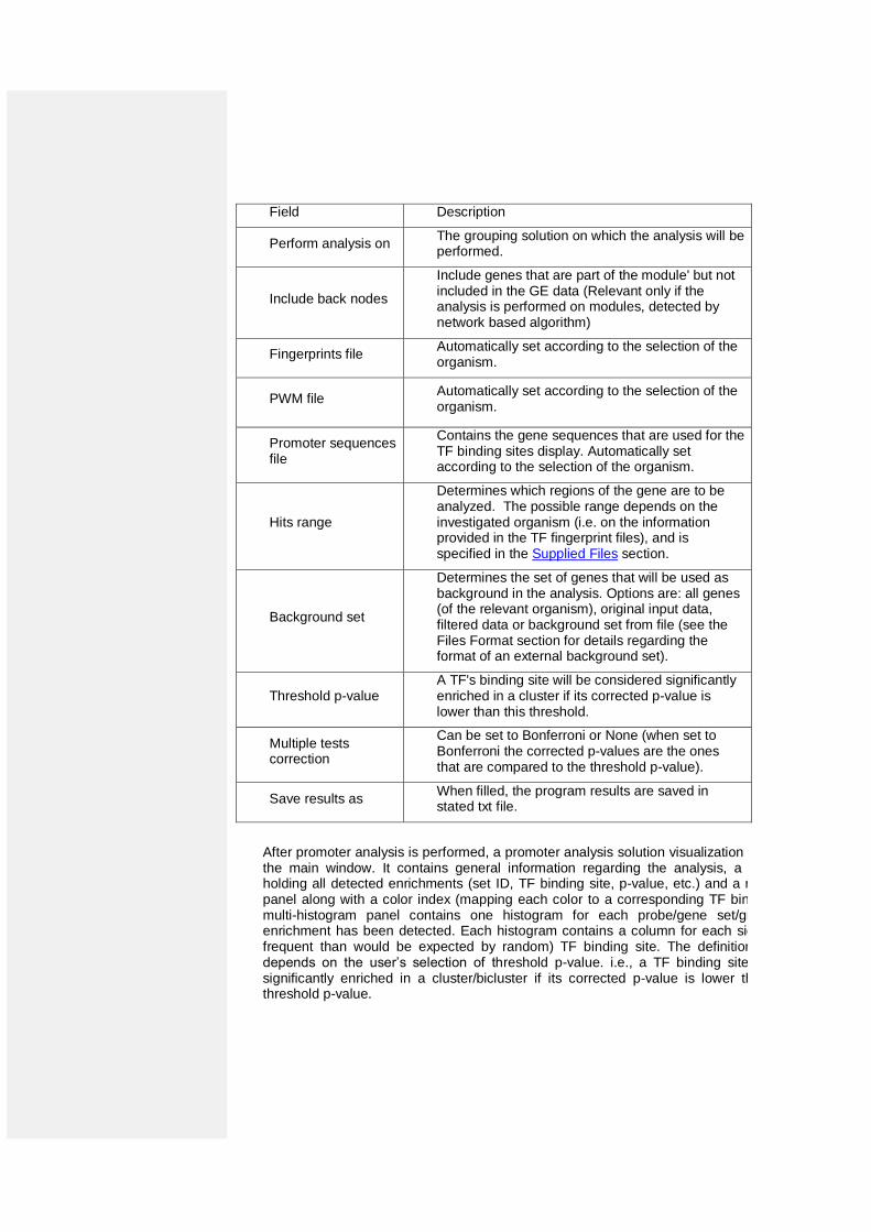
Field Description
Perform analysis on The grouping solution on which the analysis will be performed.
Include back nodes
Include genes that are part of the module' but not included in the GE data (Relevant only if the analysis is performed on modules, detected by network based algorithm)
Fingerprints file Automatically set according to the selection of the organism.
PWM file Automatically set according to the selection of the organism.
Promoter sequences file
Contains the gene sequences that are used for the TF binding sites display. Automatically set according to the selection of the organism.
Hits range
Determines which regions of the gene are to be analyzed. The possible range depends on the investigated organism (i.e. on the information provided in the TF fingerprint files), and is specified in the Supplied Files section.
Background set
Determines the set of genes that will be used as background in the analysis. Options are: all genes (of the relevant organism), original input data, filtered data or background set from file (see the Files Format section for details regarding the format of an external background set).
Threshold p-value A TF's binding site will be considered significantly enriched in a cluster if its corrected p-value is lower than this threshold.
Multiple tests correction
Can be set to Bonferroni or None (when set to Bonferroni the corrected p-values are the ones that are compared to the threshold p-value).
Save results as When filled, the program results are saved in stated txt file.
After promoter analysis is performed, a promoter analysis solution visualization tab is added to the main window. It contains general information regarding the analysis, a sort-able table holding all detected enrichments (set ID, TF binding site, p-value, etc.) and a multi-histogram panel along with a color index (mapping each color to a corresponding TF binding site). The multi-histogram panel contains one histogram for each probe/gene set/group in which enrichment has been detected. Each histogram contains a column for each significant (more frequent than would be expected by random) TF binding site. The definition of significant depends on the user’s selection of threshold p-value. i.e., a TF binding site is considered significantly enriched in a cluster/bicluster if its corrected p-value is lower than the preset threshold p-value.
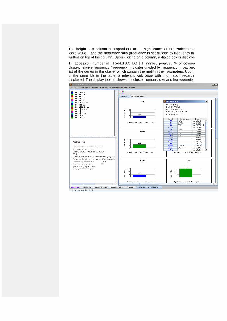
The height of a column is proportional to the significance of this enrichment (i.e. height = -log(p-value)), and the frequency ratio (frequency in set divided by frequency in background) is written on top of the column. Upon clicking on a column, a dialog box is displayed containing:
TF accession number in TRANSFAC DB [TF name], p-value, % of covered promoters in cluster, relative frequency (frequency in cluster divided by frequency in background set) and a list of the genes in the cluster which contain the motif in their promoters. Upon clicking on one of the gene Ids in the table, a relevant web page with information regarding this gene is displayed. The display tool tip shows the cluster number, size and homogeneity.
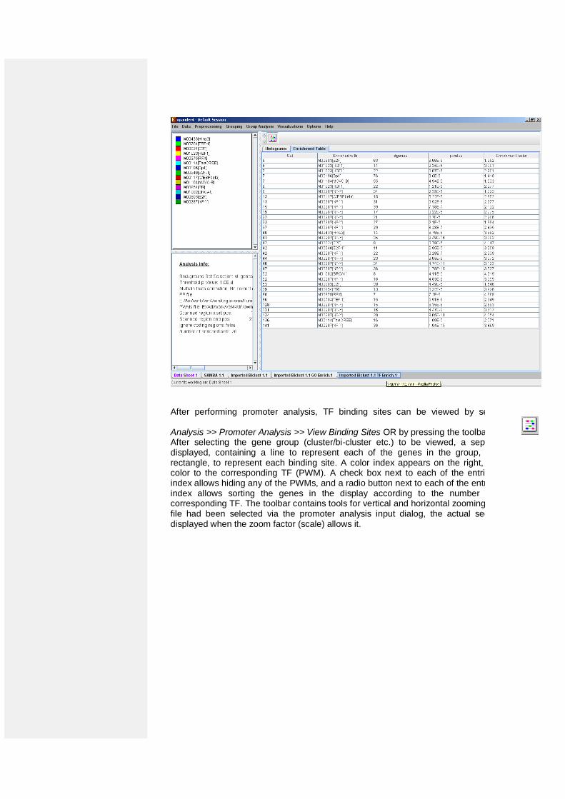
After performing promoter analysis, TF binding sites can be viewed by selecting Group
Analysis >> Promoter Analysis >> View Binding Sites OR by pressing the toolbar button ( ). After selecting the gene group (cluster/bi-cluster etc.) to be viewed, a separate frame is displayed, containing a line to represent each of the genes in the group, and a colored rectangle, to represent each binding site. A color index appears on the right, mapping each color to the corresponding TF (PWM). A check box next to each of the entries in the color index allows hiding any of the PWMs, and a radio button next to each of the entries in the color index allows sorting the genes in the display according to the number of hits of the corresponding TF. The toolbar contains tools for vertical and horizontal zooming. If a sequence file had been selected via the promoter analysis input dialog, the actual sequence will be displayed when the zoom factor (scale) allows it.
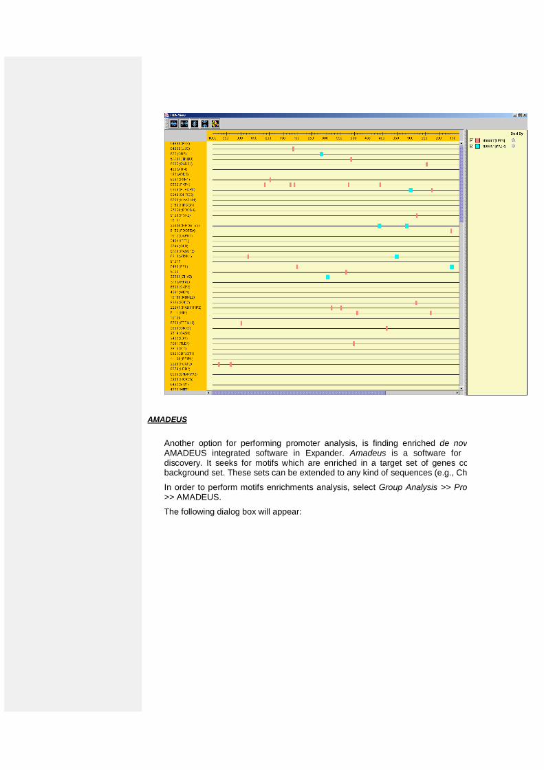
AMADEUS
Another option for performing promoter analysis, is finding enriched de novo motifs using AMADEUS integrated software in Expander. Amadeus is a software for de novo motif discovery. It seeks for motifs which are enriched in a target set of genes compared to the background set. These sets can be extended to any kind of sequences (e.g., ChIP-seq peaks).
In order to perform motifs enrichments analysis, select Group Analysis >> Promoter Analysis >> AMADEUS.
The following dialog box will appear:
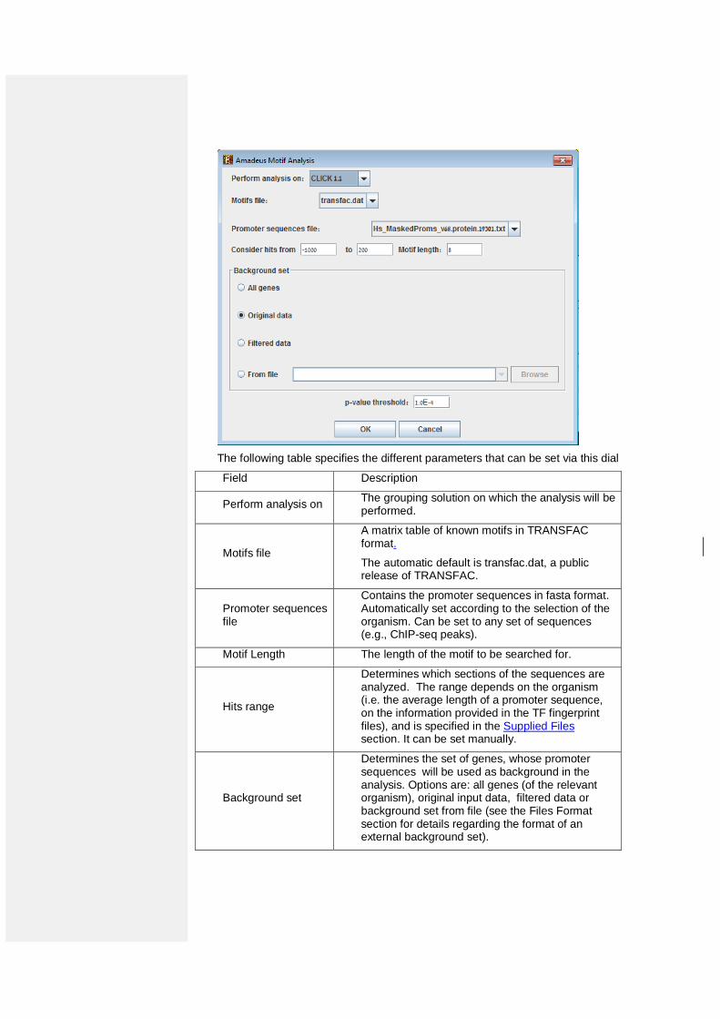
The following table specifies the different parameters that can be set via this dialog box:
Field Description
Perform analysis on The grouping solution on which the analysis will be performed.
Motifs file
A matrix table of known motifs in TRANSFAC format.
The automatic default is transfac.dat, a public release of TRANSFAC.
Promoter sequences file
Contains the promoter sequences in fasta format. Automatically set according to the selection of the organism. Can be set to any set of sequences (e.g., ChIP-seq peaks).
Motif Length The length of the motif to be searched for.
Hits range
Determines which sections of the sequences are analyzed. The range depends on the organism (i.e. the average length of a promoter sequence, on the information provided in the TF fingerprint files), and is specified in the Supplied Files section. It can be set manually.
Background set
Determines the set of genes, whose promoter sequences will be used as background in the analysis. Options are: all genes (of the relevant organism), original input data, filtered data or background set from file (see the Files Format section for details regarding the format of an external background set).
P-value threshold A motif will be considered significantly enriched in a cluster if its corrected p-value is lower than this threshold.
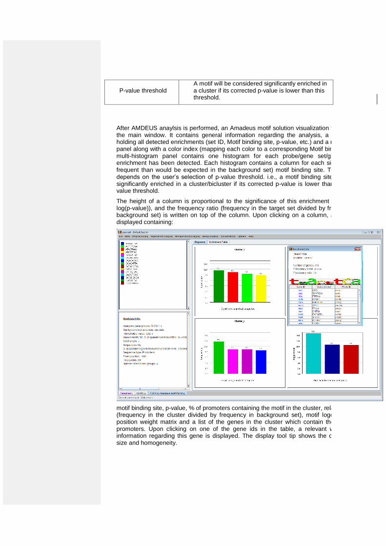
After AMDEUS anaylsis is performed, an Amadeus motif solution visualization tab is added to the main window. It contains general information regarding the analysis, a sort-able table holding all detected enrichments (set ID, Motif binding site, p-value, etc.) and a multi-histogram panel along with a color index (mapping each color to a corresponding Motif binding site). The multi-histogram panel contains one histogram for each probe/gene set/group in which enrichment has been detected. Each histogram contains a column for each significant (more frequent than would be expected in the background set) motif binding site. The significance depends on the user’s selection of p-value threshold. i.e., a motif binding site is considered significantly enriched in a cluster/bicluster if its corrected p-value is lower than the preset p-value threshold.
The height of a column is proportional to the significance of this enrichment (i.e. height = -log(p-value)), and the frequency ratio (frequency in the target set divided by frequency in the background set) is written on top of the column. Upon clicking on a column, a dialog box is displayed containing:
motif binding site, p-value, % of promoters containing the motif in the cluster, relative frequency (frequency in the cluster divided by frequency in background set), motif logo created from position weight matrix and a list of the genes in the cluster which contain the motif in their promoters. Upon clicking on one of the gene ids in the table, a relevant web page with information regarding this gene is displayed. The display tool tip shows the cluster number, size and homogeneity.
TF motif fingerprint files and promoter sequence files are currently supplied with EXPANDER for yeast, human, mouse, rat, fly, zebrafish, c-elegans, arabidopsis and chicken, and are updated on a regular basis (for more information, refer to the Supplied Files section).
The results of this analysis can be exported to a text by selecting File>>Export to text when the corresponding view is the selected tab.
Location Enrichment Analysis
This tool performs basic statistical analysis on the distribution of chromosomal locations of genes within each group. The locations of the genes are specified in organism-specific data files, which can be downloaded from the EXPANDER download-page (see the Supplied Files section).
Before operating location analysis, the location data for the relevant organism should be
downloaded from the download page (more details at introduction of Group Analysis Tools).
In this analysis, hyper-geometric enrichment tests are performed, and the results can be (if requested) corrected for multiple testing using the Bonferroni correction.
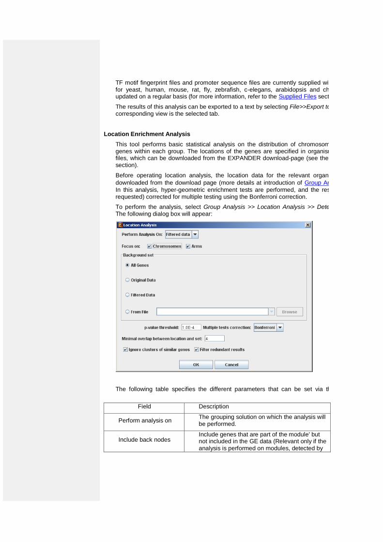
To perform the analysis, select Group Analysis >> Location Analysis >> Detect Enrichment. The following dialog box will appear:
The following table specifies the different parameters that can be set via this dialog box:
Field Description
Perform analysis on The grouping solution on which the analysis will be performed.
Include back nodes Include genes that are part of the module' but not included in the GE data (Relevant only if the analysis is performed on modules, detected by
network based algorithm)
Focus on (Chromosomes, Arms*, Bands*)
Location types to perform analysis on.
Background set
Determines the set of genes that will be used as background in the analysis. Options are: all genes (of the relevant organism), original input data, filtered data or background set from file (see the Files Format section for details regarding the format of an external background set).
p-value threshold A category/attribute will be considered significantly enriched in a cluster/bicluster if its corrected p-value is lower than this threshold.
Multiple tests correction
Can be set to Bonferroni or None (when set to Bonferroni the corrected p-values are the ones that are compared to the threshold p-value).
Minimal overlap between category and set
The minimal number of genes from a group (cluster/bi-cluster/module etc.) expected to be categorized/attributed by an attribute in order for its enrichment to be accepted.
Ignore clusters of similar genes*
If selected, genes from known homology clusters are not included in the analysis.
Filter redundant results
If selected, the results are filtered, so that out of two enrichments of overlapping areas in the same group, only one is selected (the most significant one).
* If relevant data exists
After the analysis is performed an enrichment analysis solution visualization tab is added to the main window. It contains general information regarding the analysis, a sort-able table holding all detected enrichments (set ID, enrichment category, p-value, etc.) and a multi-histogram panel along with a color index (mapping each color to a corresponding location). The multi-histogram panel contains one histogram for each probe/gene group in which enrichment has been detected. Each histogram contains a column for each significant (more frequent than would be expected by random) location. The definition of significant depends on the user’s selection of threshold p-value i.e., a category is considered significantly enriched in a cluster/bicluster if its corrected p-value is lower than the preset threshold p-value.
The height of the column is proportional to the significance of this enrichment (i.e. height = -log(raw p-value)), and the frequency ratio (frequency in set divided by frequency in background) is written on top of the column. Upon clicking on a column, a dialog box is displayed containing the location, corrected p-value, and a list of the genes in the group that are mapped to this location. Upon clicking on one of the gene Ids in the table, a relevant web page with information regarding this gene is displayed.
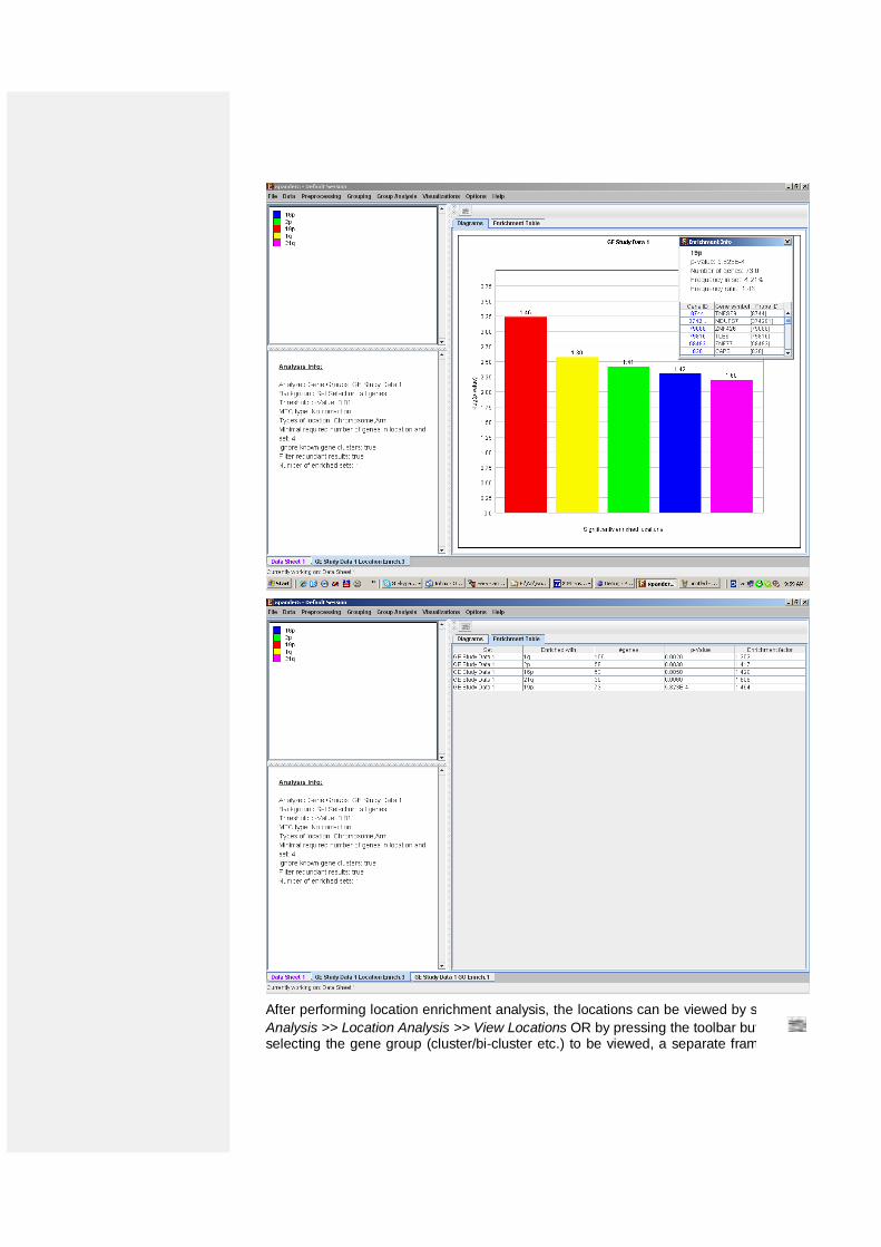
After performing location enrichment analysis, the locations can be viewed by selecting Group
Analysis >> Location Analysis >> View Locations OR by pressing the toolbar button ( ). After selecting the gene group (cluster/bi-cluster etc.) to be viewed, a separate frame is displayed,
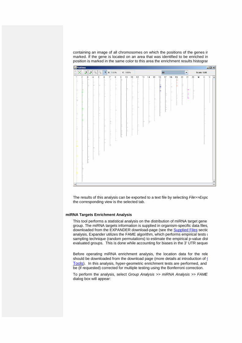
containing an image of all chromosomes on which the positions of the genes in the group are marked. If the gene is located on an area that was identified to be enriched in that group, its position is marked in the same color to this area the enrichment results histogram.
The results of this analysis can be exported to a text file by selecting File>>Export to text when the corresponding view is the selected tab.
miRNA Targets Enrichment Analysis
This tool performs a statistical analysis on the distribution of miRNA target gene within each group. The miRNA targets information is supplied in organism-specific data files, which can be downloaded from the EXPANDER download-page (see the Supplied Files section). For this analysis, Expander utilizes the FAME algorithm, which performs empirical tests using a sampling technique (random permutations) to estimate the empirical p-value distribution for the evaluated groups. This is done while accounting for biases in the 3' UTR sequences
Before operating miRNA enrichment analysis, the location data for the relevant organism
should be downloaded from the download page (more details at introduction of Group Analysis Tools). In this analysis, hyper-geometric enrichment tests are performed, and the results can be (if requested) corrected for multiple testing using the Bonferroni correction.
To perform the analysis, select Group Analysis >> miRNA Analysis >> FAME. The following dialog box will appear:
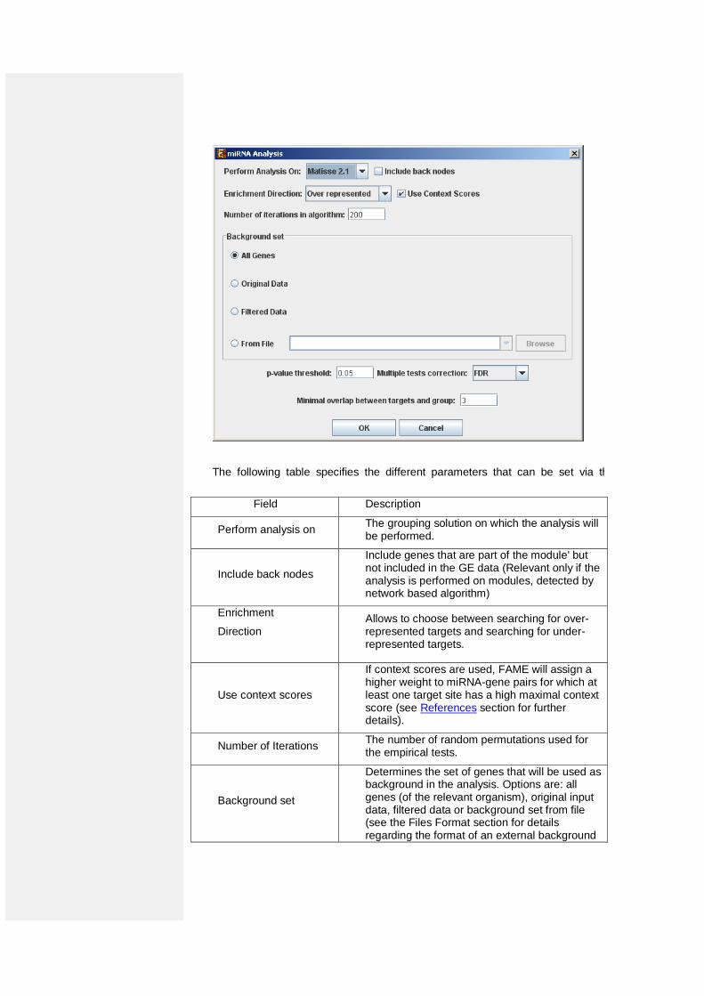
The following table specifies the different parameters that can be set via this dialog box:
Field Description
Perform analysis on The grouping solution on which the analysis will be performed.
Include back nodes
Include genes that are part of the module' but not included in the GE data (Relevant only if the analysis is performed on modules, detected by network based algorithm)
Enrichment
Direction
Allows to choose between searching for over-represented targets and searching for under-represented targets.
Use context scores
If context scores are used, FAME will assign a higher weight to miRNA-gene pairs for which at least one target site has a high maximal context score (see References section for further details).
Number of Iterations The number of random permutations used for the empirical tests.
Background set
Determines the set of genes that will be used as background in the analysis. Options are: all genes (of the relevant organism), original input data, filtered data or background set from file (see the Files Format section for details regarding the format of an external background
set).
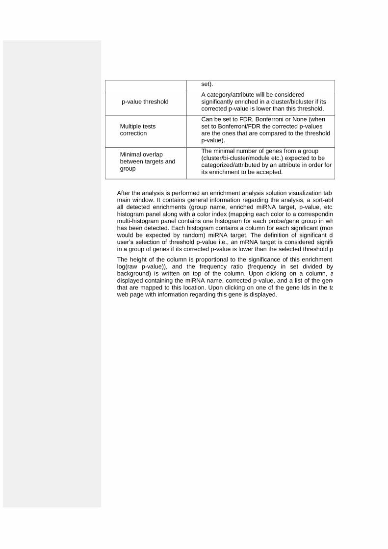
p-value threshold A category/attribute will be considered significantly enriched in a cluster/bicluster if its corrected p-value is lower than this threshold.
Multiple tests correction
Can be set to FDR, Bonferroni or None (when set to Bonferroni/FDR the corrected p-values are the ones that are compared to the threshold p-value).
Minimal overlap between targets and group
The minimal number of genes from a group (cluster/bi-cluster/module etc.) expected to be categorized/attributed by an attribute in order for its enrichment to be accepted.
After the analysis is performed an enrichment analysis solution visualization tab is added to the main window. It contains general information regarding the analysis, a sort-able table holding all detected enrichments (group name, enriched miRNA target, p-value, etc.) and a multi-histogram panel along with a color index (mapping each color to a corresponding miRNA). The multi-histogram panel contains one histogram for each probe/gene group in which enrichment has been detected. Each histogram contains a column for each significant (more frequent than would be expected by random) miRNA target. The definition of significant depends on the user’s selection of threshold p-value i.e., an mRNA target is considered significantly enriched in a group of genes if its corrected p-value is lower than the selected threshold p-value.
The height of the column is proportional to the significance of this enrichment (i.e. height = -log(raw p-value)), and the frequency ratio (frequency in set divided by frequency in background) is written on top of the column. Upon clicking on a column, a dialog box is displayed containing the miRNA name, corrected p-value, and a list of the genes in the group that are mapped to this location. Upon clicking on one of the gene Ids in the table, a relevant web page with information regarding this gene is displayed.
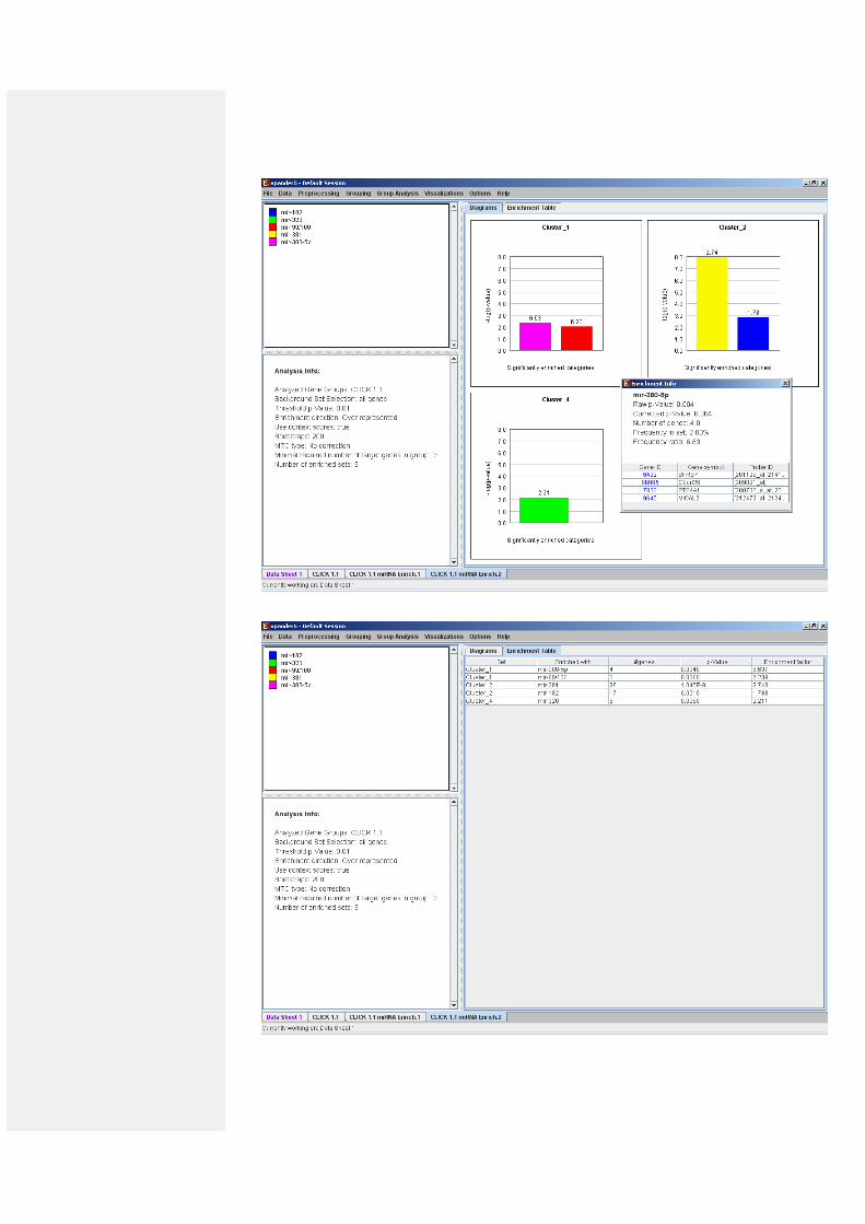
The results of this analysis can be exported to a text file by selecting File>>Export to text when the corresponding view is the selected tab.
Pathway Enrichment Analysis
This tool performs a statistical analysis on the representation of KEGG and WikiPathways pathway maps within each group. The KEGG and WikiPathways information is supplied in organism-specific data files, which can be downloaded from the EXPANDER download-page (see the Supplied Files section In this analysis, hyper-geometric enrichment tests are performed, and the results can be (if requested) corrected for multiple testing using the Bonferroni correction.
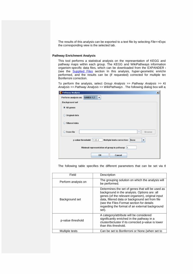
To perform the analysis, select Group Analysis >> Pathway Analysis >> KEGG or Group Analysis >> Pathway Analysis >> WikiPathways . The following dialog box will appear:
The following table specifies the different parameters that can be set via this dialog box:
Field Description
Perform analysis on The grouping solution on which the analysis will be performed.
Background set
Determines the set of genes that will be used as background in the analysis. Options are: all genes (of the relevant organism), original input data, filtered data or background set from file (see the Files Format section for details regarding the format of an external background set).
p-value threshold
A category/attribute will be considered significantly enriched in the pathway in a cluster/bicluster if its corrected p-value is lower than this threshold.
Multiple tests Can be set to Bonferroni or None (when set to
correction Bonferroni the corrected p-values are the ones that are compared to the threshold p-value).
Minimal overlap between category and set
The minimal number of genes from a cluster/bi-cluster expected to be categorized/attributed by an attribute in order for its pathway analysis to be accepted.
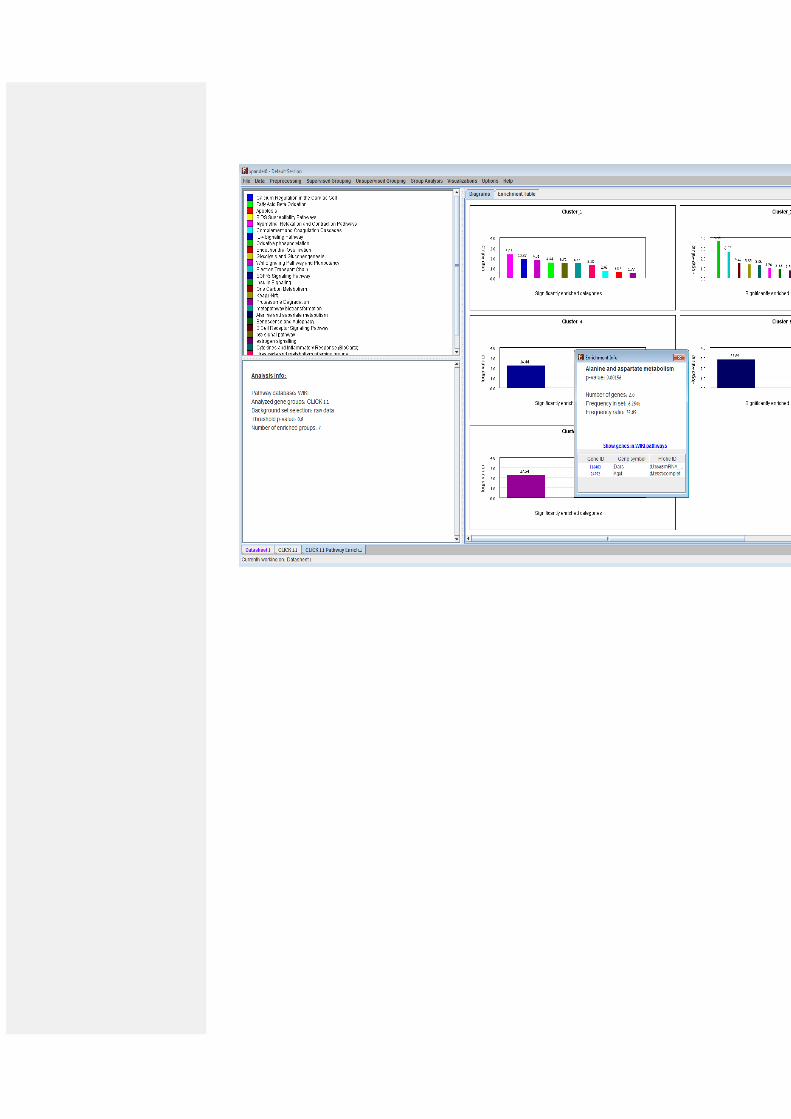
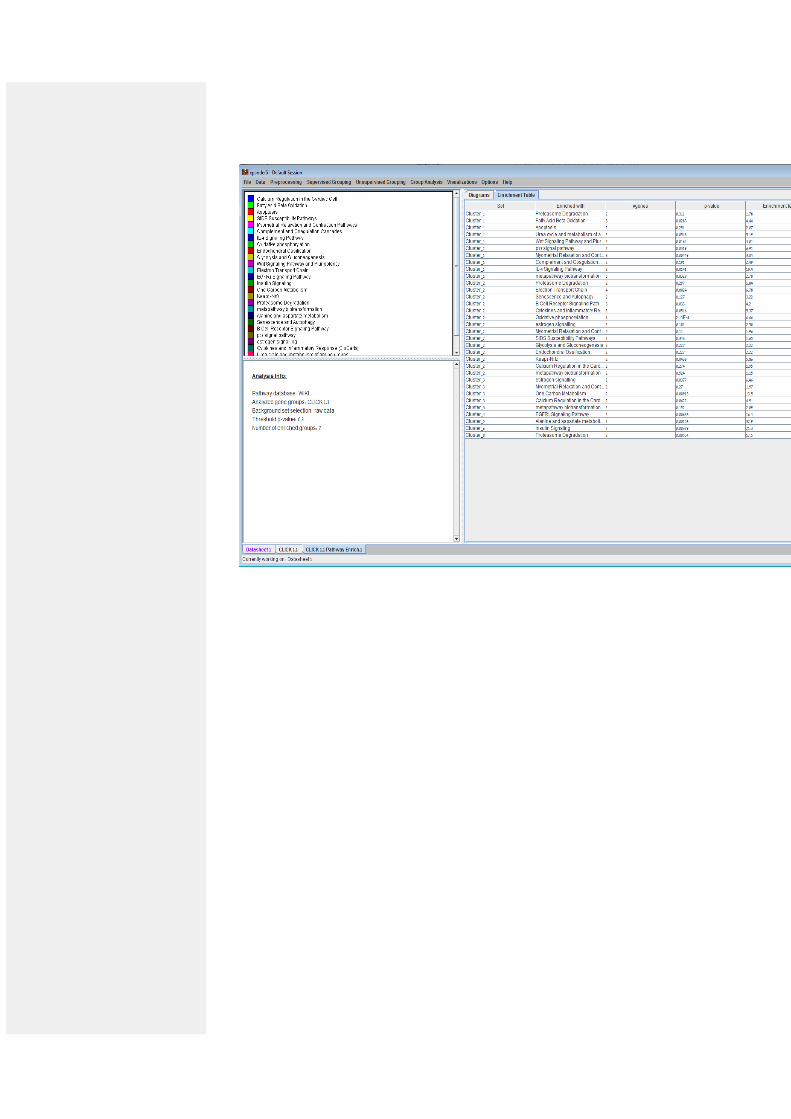
After the analysis was performed a Pathway analysis solution visualization tab is added to the
main window. It contains general information about the analysis, a sorted table holding all detected pathways (group name, enriched pathway target, p-value, etc.) and multi-histogram panel along with a color index (mapping each color to a corresponding pathway). The multi-histogram panel contains one histogram for each probe/gene group in which enrichment has been detected. Each histogram contains a column for each significant (more frequent than would be expected by random) pathway target. The definition of significant depends on the user’s selection of threshold p-value i.e., a pathway target is considered significantly enriched in a group of genes if its corrected p-value is lower than the selected threshold p-value.
The height of the column is proportional to the significance of this enrichment (i.e. height = -log(raw p-value)), and the frequency ratio (frequency in set divided by frequency in background) is written on top of the column. Upon clicking on a column, a dialog box is displayed containing the pathway name, corrected p-value, link to the relevant pathway map web page, and a list of the genes in the group that are included in the corresponding pathway. Upon clicking on one of the gene Ids in the table, a relevant web page with information regarding this gene is displayed. Upon clicking on the link to the pathway map web page, the web browser displays the page with the relevant genes highlighted in it.
General Enrichment Analysis
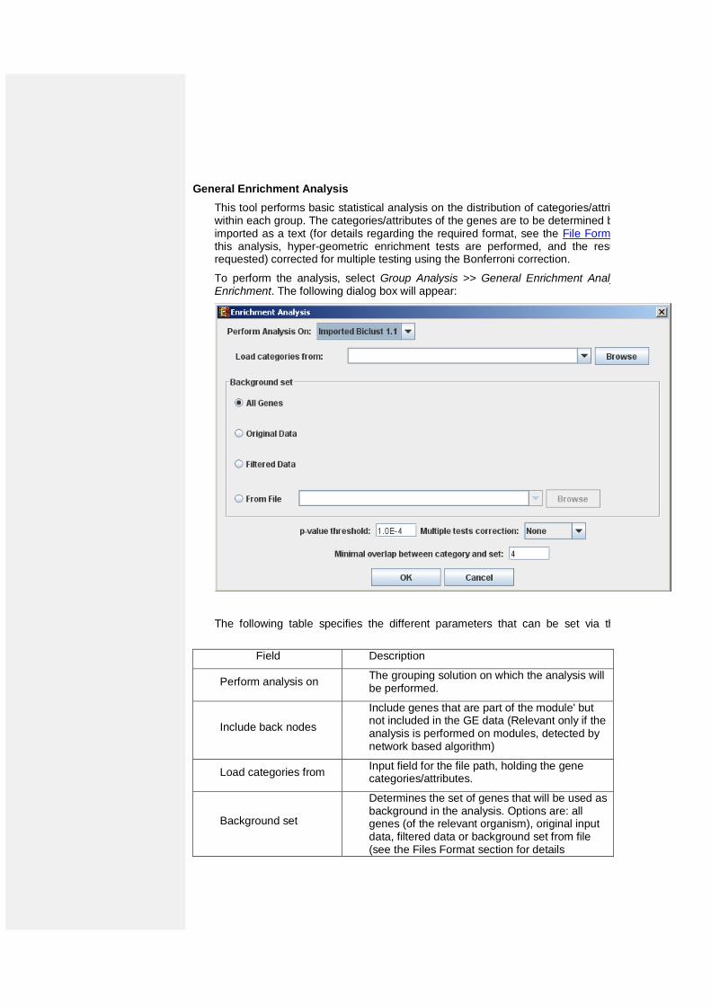
This tool performs basic statistical analysis on the distribution of categories/attributes of genes within each group. The categories/attributes of the genes are to be determined by the user and imported as a text (for details regarding the required format, see the File Formats section). In this analysis, hyper-geometric enrichment tests are performed, and the results can be (if requested) corrected for multiple testing using the Bonferroni correction.
To perform the analysis, select Group Analysis >> General Enrichment Analysis >> Detect Enrichment. The following dialog box will appear:
The following table specifies the different parameters that can be set via this dialog box:
Field Description
Perform analysis on The grouping solution on which the analysis will be performed.
Include back nodes
Include genes that are part of the module' but not included in the GE data (Relevant only if the analysis is performed on modules, detected by network based algorithm)
Load categories from Input field for the file path, holding the gene categories/attributes.
Background set
Determines the set of genes that will be used as background in the analysis. Options are: all genes (of the relevant organism), original input data, filtered data or background set from file (see the Files Format section for details
regarding the format of an external background set).
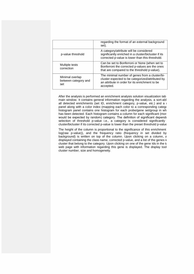
p-value threshold A category/attribute will be considered significantly enriched in a cluster/bicluster if its corrected p-value is lower than this threshold.
Multiple tests correction
Can be set to Bonferroni or None (when set to Bonferroni the corrected p-values are the ones that are compared to the threshold p-value).
Minimal overlap between category and set
The minimal number of genes from a cluster/bi-cluster expected to be categorized/attributed by an attribute in order for its enrichment to be accepted.
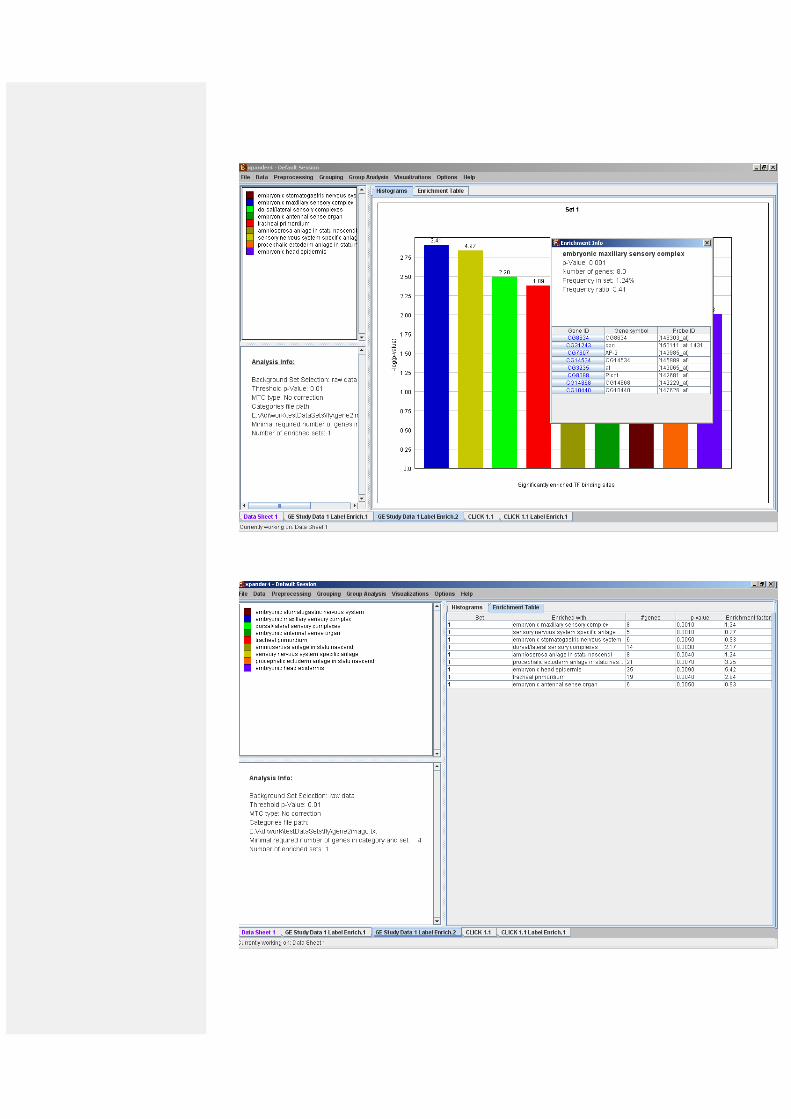
After the analysis is performed an enrichment analysis solution visualization tab is added to the main window. It contains general information regarding the analysis, a sort-able table holding all detected enrichments (set ID, enrichment category, p-value, etc.) and a multi-histogram panel along with a color index (mapping each color to a corresponding category). The multi-histogram panel contains one histogram for each probe/gene set/group in which enrichment has been detected. Each histogram contains a column for each significant (more frequent than would be expected by random) category. The definition of significant depends on the user’s selection of threshold p-value i.e., a category is considered significantly enriched in a cluster/bicluster if its corrected p-value is lower than the preset threshold p-value.
The height of the column is proportional to the significance of this enrichment (i.e. height = -log(raw p-value)), and the frequency ratio (frequency in set divided by frequency in background) is written on top of the column. Upon clicking on a column, a dialog box is displayed containing the class name, corrected p-value, and a list of the genes in the cluster/bi-cluster that belong to the category. Upon clicking on one of the gene Ids in the table, a relevant web page with information regarding this gene is displayed. The display tool tip shows the cluster number, size and homogeneity.
The results of this analysis can be exported to a text file by selecting File>>Export to text when the corresponding view is the selected tab.
Network Based Group Analysis
This tool allows browsing through signaling data to view the sub-graphs that are induced by the analyzed gene groups. It also enables the user to search for statistical enrichment of these groups in highly curated signaling maps. To perform this task, Expander interfaces with the SPIKE software and database. For further information regarding the SPIKE software see the References section.
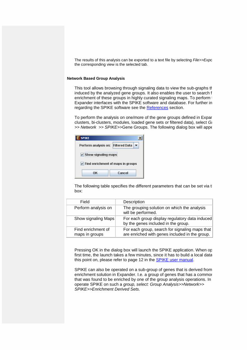
To perform the analysis on one/more of the gene groups defined in Expander (i.e. clusters, bi-clusters, modules, loaded gene sets or filtered data), select Group Analysis >> Network >> SPIKE>>Gene Groups. The following dialog box will appear:
The following table specifies the different parameters that can be set via this dialog box:
Field Description
Perform analysis on The grouping solution on which the analysis will be performed.
Show signaling Maps For each group display regulatory data induced by the genes included in the group.
Find enrichment of maps in groups
For each group, search for signaling maps that are enriched with genes included in the group.
Pressing OK in the dialog box will launch the SPIKE application. When operated for the first time, the launch takes a few minutes, since it has to build a local database. From this point on, please refer to page 12 in the SPIKE user manual.
SPIKE can also be operated on a sub-group of genes that is derived from an existing enrichment solution in Expander. I.e. a group of genes that has a common annotation that was found to be enriched by one of the group analysis operations. In order to operate SPIKE on such a group, select: Group Analysis>>Network>> SPIKE>>Enrichment Derived Sets.
Gene Set Enrichment Analysis (GSEA)
GSEA (Subramanian et al 2005) considers experiments with genomewide expression profiles from samples belonging to two classes, labeled "MUT" or "WT". Genes are ranked based on the correlation between their expression and the differential expression between classes distinction or pre-ranked by the user. Given an a priori defined set of genes S, the goal of GSEA is to determine whether the members of S are randomly distributed throughout the ranked list of genes (L) or primarily found at the top or bottom. It is expected that sets related to the phenotypic distinction will tend to show the latter distribution. There are two key elements of the GSEA method in Expander: Step 1: Calculation of an Enrichment Score. Enrichment score (ES) reflects the degree to which a set S is overrepresented at the extremes (top or bottom) of the entire ranked list L. The score is calculated by walking down the list L, increasing a running-sum statistic when we encounter a gene in S and decreasing it when we encounter genes not in S. The magnitude of the increment depends on the correlation of the gene with the phenotype. The enrichment score is the maximum deviation from zero encountered in the random walk. It corresponds to a weighted Kolmogorov–Smirnov-like statistic. Step 2: Estimation of Significance Level of ES. An estimation of the statistical significance (nominal P-value) of the ES is done by using an empirical phenotype-based permutation test procedure that preserves the complex correlation structure of the gene expression data. Specifically, the phenotype labels are permuted again and the ES of the gene set for the permuted data is re-computed, which generates a null distribution for the ES. If the user provided a pre-ranked list of genes then a random shuffling of the ranked list is done instead. The empirical, nominal P value of the observed ES is then calculated relative to this null distribution. Importantly, the permutation of class labels preserves gene-gene correlations and, thus, provides a more biologically reasonable assessment of significance than would be obtained by permuting genes.
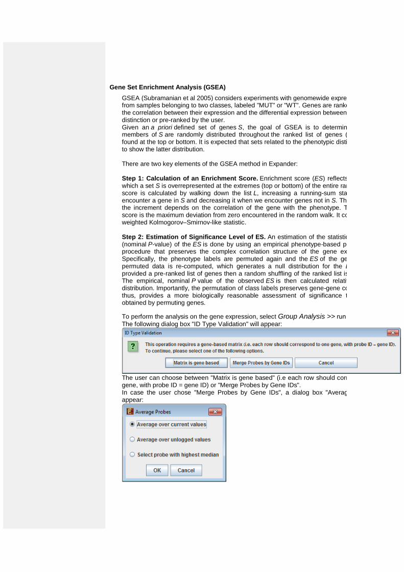
To perform the analysis on the gene expression, select Group Analysis >> run GSEA…
The following dialog box "ID Type Validation" will appear:
The user can choose between "Matrix is gene based" (i.e each row should correspond to one gene, with probe ID = gene ID) or "Merge Probes by Gene IDs". In case the user chose "Merge Probes by Gene IDs", a dialog box "Average Probes" will appear:
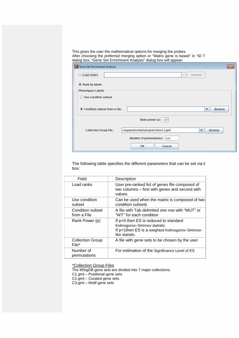
This gives the user the mathematical options for merging the probes. After choosing the preferred merging option or "Matrix gene is based" in "ID Type Validation" dialog box, "Gene Set Enrichment Analysis" dialog box will appear:
The following table specifies the different parameters that can be set via this dialog box:
Field Description
Load ranks User pre-ranked list of genes file composed of two columns – first with genes and second with values
Use condition subset
Can be used when the matrix is composed of two condition subsets
Condition subset from a File
A file with Tab delimited one row with "MUT" or "WT" for each condition
Rank Power (p) If p=0 then ES is reduced to standard Kolmogorov–Smirnov statistic. If p=1then ES is a weighted Kolmogorov–Smirnov-
like statistic.
Collection Group File*
A file with gene sets to be chosen by the user
Number of permutations
For estimation of the Significance Level of ES
*Collection Group Files The MSigDB gene sets are divided into 7 major collections: C1.gmt – Positional gene sets C2.gmt – Curated gene sets C3.gmt – Motif gene sets
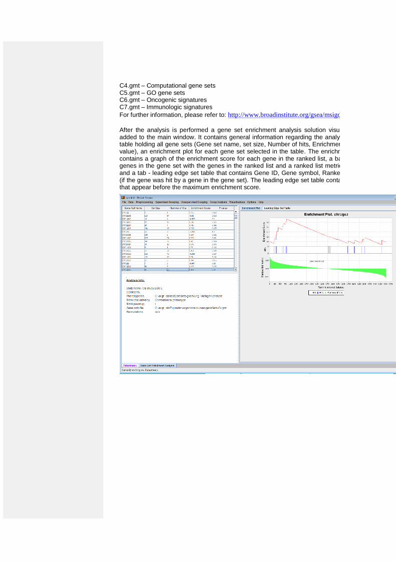
C4.gmt – Computational gene sets C5.gmt – GO gene sets C6.gmt – Oncogenic signatures C7.gmt – Immunologic signatures
For further information, please refer to: http://www.broadinstitute.org/gsea/msigdb/index.jsp
After the analysis is performed a gene set enrichment analysis solution visualization tab is added to the main window. It contains general information regarding the analysis, a sort-able table holding all gene sets (Gene set name, set size, Number of hits, Enrichment score and P-value), an enrichment plot for each gene set selected in the table. The enrichment plot panel contains a graph of the enrichment score for each gene in the ranked list, a bar of hits of the genes in the gene set with the genes in the ranked list and a ranked list metric of the genes, and a tab - leading edge set table that contains Gene ID, Gene symbol, Ranke metric and Hit (if the gene was hit by a gene in the gene set). The leading edge set table contains only genes that appear before the maximum enrichment score.
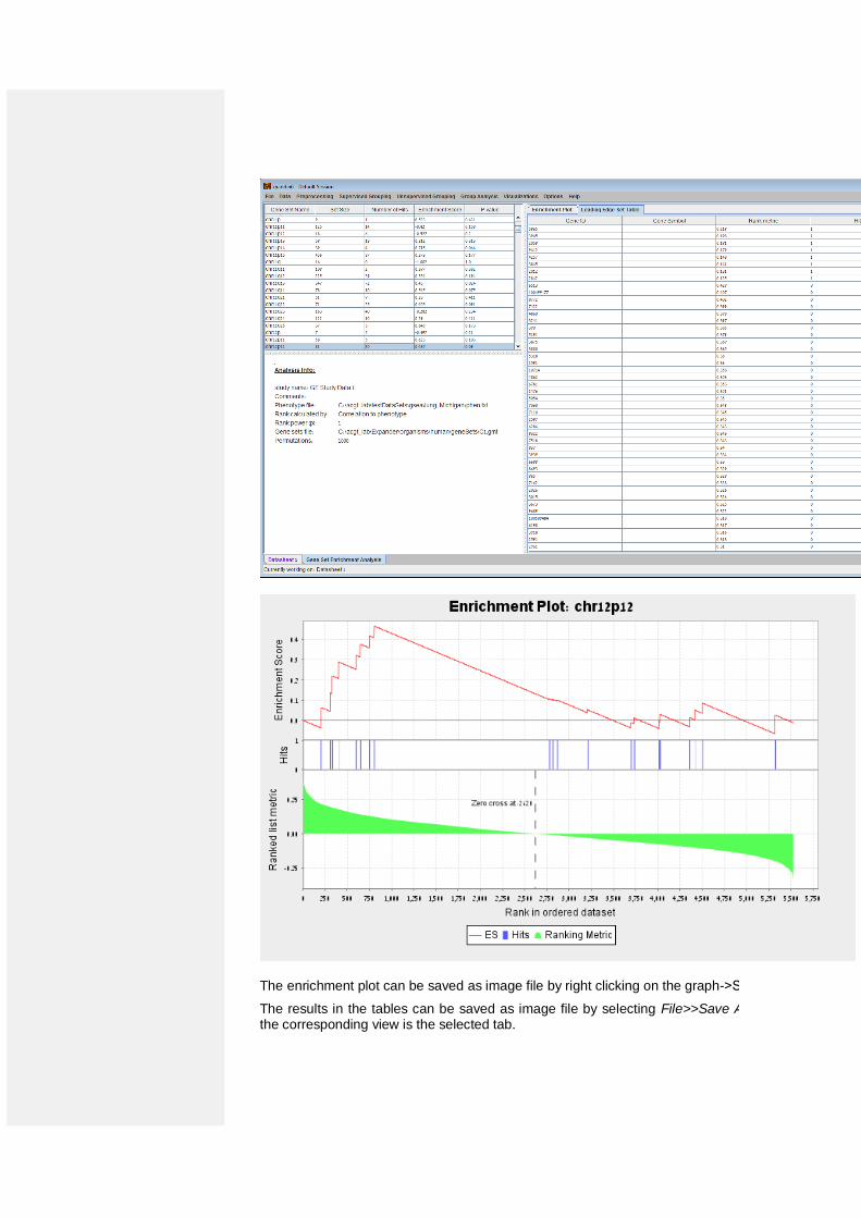
The enrichment plot can be saved as image file by right clicking on the graph->Save as…
The results in the tables can be saved as image file by selecting File>>Save As Image when the corresponding view is the selected tab.
Matrix Visualizations
An expression matrix (Heat-map) visualization is integrated in many of EXPANDER’s displays. This visualization is similar to the red-green matrix representation of Eisen et al (1998). All it does is to render the gene-expression data on the screen in color, where green indicates under expression, and red indicates over expression. Color rendering can be configured by the user in one of the following manners: (a) by setting the range (top and bottom values) of rendered values (default values are set according to the data scale, e.g. 40-1000 for non-standardized absolute intensities data) or (b) by setting the percent of values, which are to be disregarded as extreme values from each edge (by default set to 5%). The manner of color scale configuration (i.e. (a) vs. (b)) can be set via the ‘Data Matrix View’ tab in the ‘Display Settings’ dialog box, available from Options >> Settings. The red/green coloring scheme can be changed to blue/yellow (using Options >> Settings >> Display >> ‘Data Matrix View’ tab).
A color scale appears next to the matrix (upper right side). The displayed tool tip shows the probe ID and condition title corresponding to the row and column on which the cursor is placed, and the expression value in that position. The matrix toolbar contains zoom in, zoom out, reset scale (to reset zoom factor), shorten condition title and Elongate condition title tools.
Upon selecting Visualizations >> Clustered Expression Matrix, a clustered expression matrix visualization tab is added to the main window. The probes are ordered in their original order. If a clustering solution has been previously created, its’ name appears next to a radio button in the top right panel. Upon pressing this button, the order of the probes in the display changes and probe IDs are colored according to the clusters. The color index at the bottom right panel, maps each color to the index of the corresponding cluster.
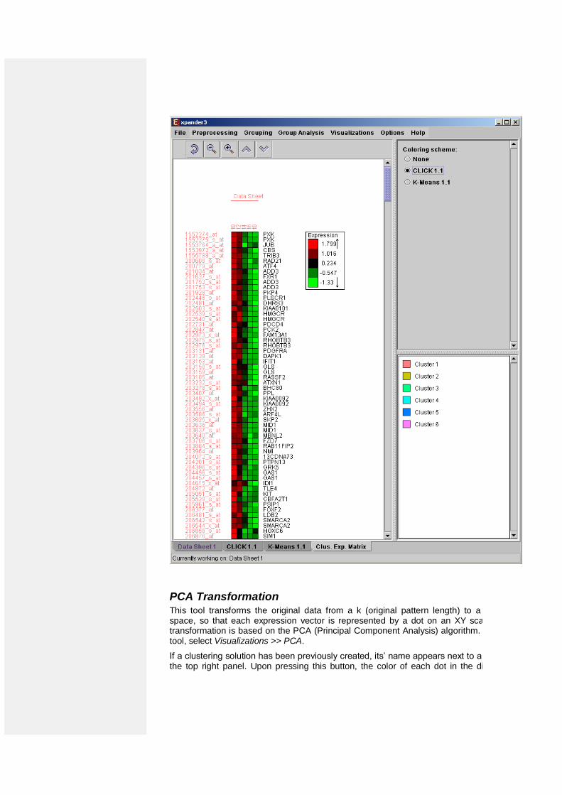
PCA Transformation
This tool transforms the original data from a k (original pattern length) to a 2 dimensional space, so that each expression vector is represented by a dot on an XY scatter chart. The transformation is based on the PCA (Principal Component Analysis) algorithm. To operate the tool, select Visualizations >> PCA.
If a clustering solution has been previously created, its’ name appears next to a radio button in the top right panel. Upon pressing this button, the color of each dot in the display changes
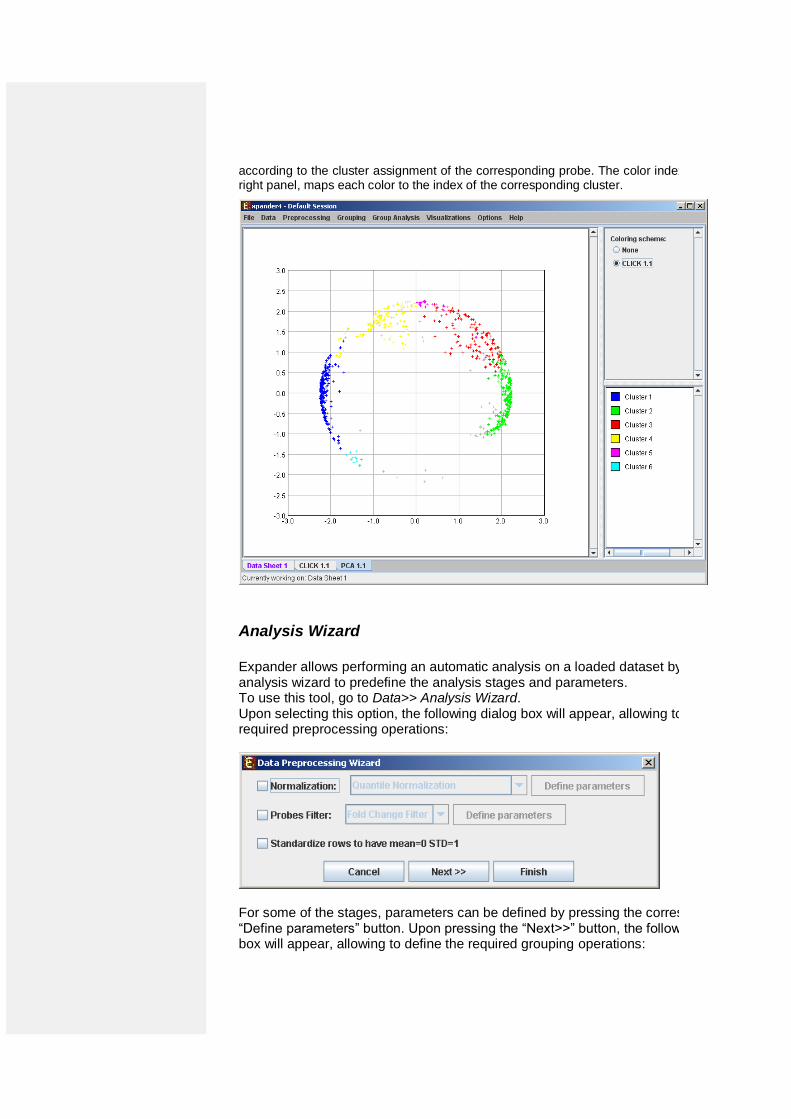
according to the cluster assignment of the corresponding probe. The color index at the bottom right panel, maps each color to the index of the corresponding cluster.
Analysis Wizard
Expander allows performing an automatic analysis on a loaded dataset by using the analysis wizard to predefine the analysis stages and parameters. To use this tool, go to Data>> Analysis Wizard. Upon selecting this option, the following dialog box will appear, allowing to define the required preprocessing operations:
For some of the stages, parameters can be defined by pressing the corresponding “Define parameters” button. Upon pressing the “Next>>” button, the following dialog box will appear, allowing to define the required grouping operations:
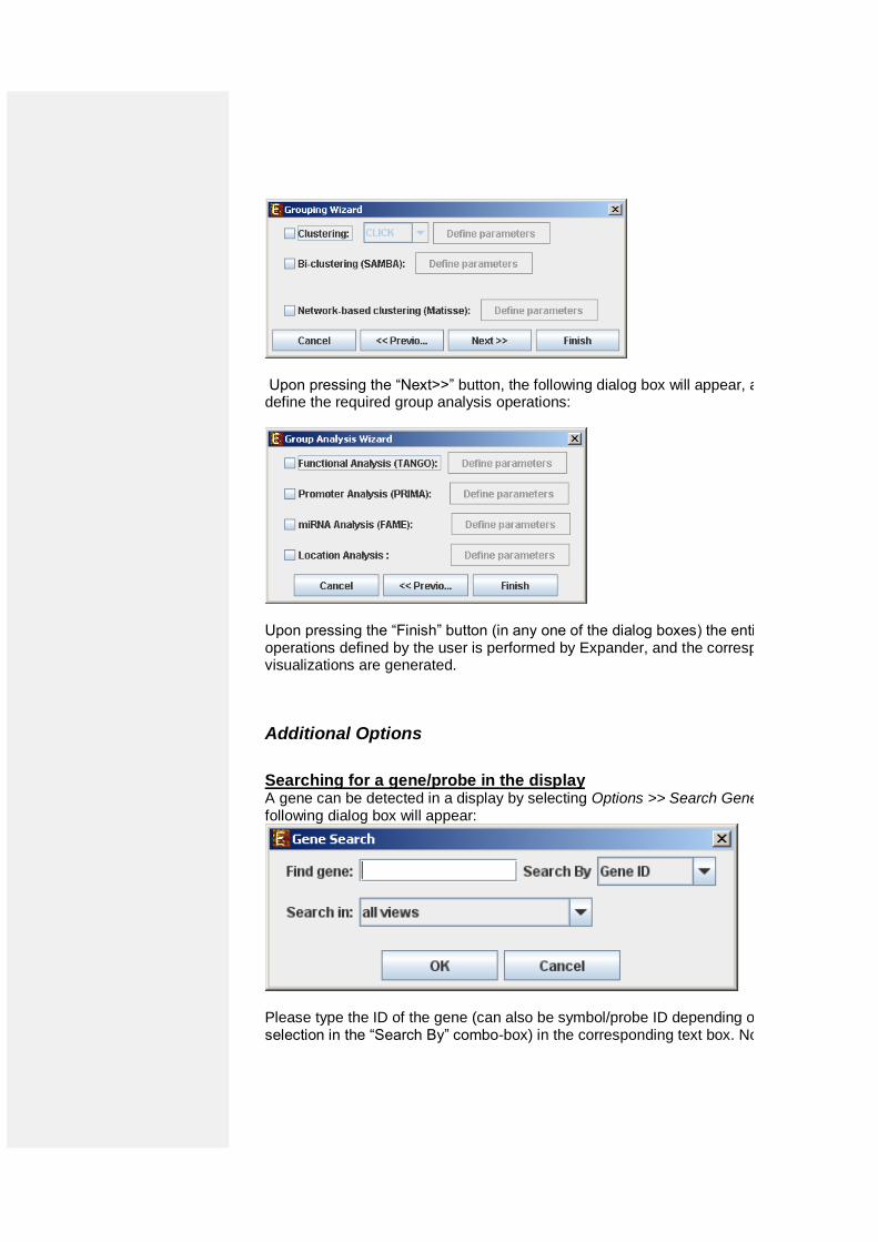
Upon pressing the “Next>>” button, the following dialog box will appear, allowing to define the required group analysis operations:
Upon pressing the “Finish” button (in any one of the dialog boxes) the entire set of operations defined by the user is performed by Expander, and the corresponding visualizations are generated.
Additional Options
Searching for a gene/probe in the display A gene can be detected in a display by selecting Options >> Search Gene. The following dialog box will appear:
Please type the ID of the gene (can also be symbol/probe ID depending on the selection in the “Search By” combo-box) in the corresponding text box. Note that you
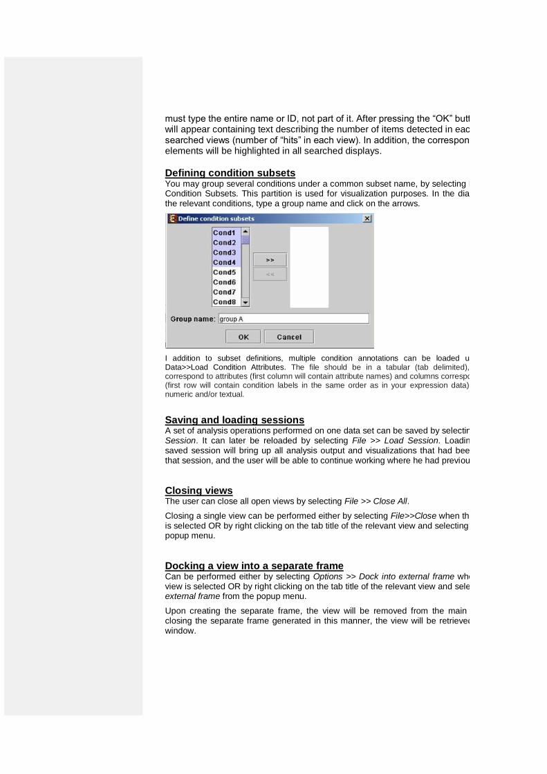
must type the entire name or ID, not part of it. After pressing the “OK” button, a window will appear containing text describing the number of items detected in each of the searched views (number of “hits” in each view). In addition, the corresponding elements will be highlighted in all searched displays.
Defining condition subsets You may group several conditions under a common subset name, by selecting Data >> Define Condition Subsets. This partition is used for visualization purposes. In the dialog box, select the relevant conditions, type a group name and click on the arrows.
I addition to subset definitions, multiple condition annotations can be loaded using the option Data>>Load Condition Attributes. The file should be in a tabular (tab delimited), in which rows correspond to attributes (first column will contain attribute names) and columns correspond to conditions (first row will contain condition labels in the same order as in your expression data). Values can be numeric and/or textual.
Saving and loading sessions A set of analysis operations performed on one data set can be saved by selecting File >> Save Session. It can later be reloaded by selecting File >> Load Session. Loading a previously saved session will bring up all analysis output and visualizations that had been generated in that session, and the user will be able to continue working where he had previously stopped.
Closing views The user can close all open views by selecting File >> Close All.
Closing a single view can be performed either by selecting File>>Close when the relevant view is selected OR by right clicking on the tab title of the relevant view and selecting Close from the popup menu.
Docking a view into a separate frame Can be performed either by selecting Options >> Dock into external frame when the relevant view is selected OR by right clicking on the tab title of the relevant view and selecting Dock into external frame from the popup menu.
Upon creating the separate frame, the view will be removed from the main window. Upon closing the separate frame generated in this manner, the view will be retrieved into the main window.
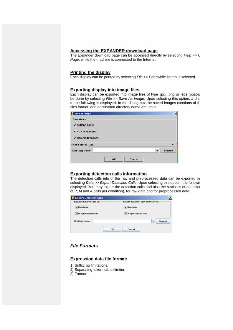
Accessing the EXPANDER download page The Expander download page can be accessed directly by selecting Help >> Open Download Page, while the machine is connected to the Internet.
Printing the display Each display can be printed by selecting File >> Print while its tab is selected.
Exporting display into image files Each display can be exported into image files of type .jpg, .png or .eps (post-script). This can be done by selecting File >> Save As Image. Upon selecting this option, a dialog box, similar to the following is displayed. In the dialog box the saved images (sections of the view), image files format, and destination directory name are input.
Exporting detection calls information The detection calls info of the raw and preprocessed data can be exported into text files, by selecting Data >> Export Detection Calls. Upon selecting this option, the following dialog box is displayed. You may export the detection calls and also the statistics of detection calls (percent of P, M and A calls per condition), for raw data and for preprocessed data.
File Formats
Expression data file format:
1) Suffix: no limitations. 2) Separating token: tab delimiter. 3) Format:
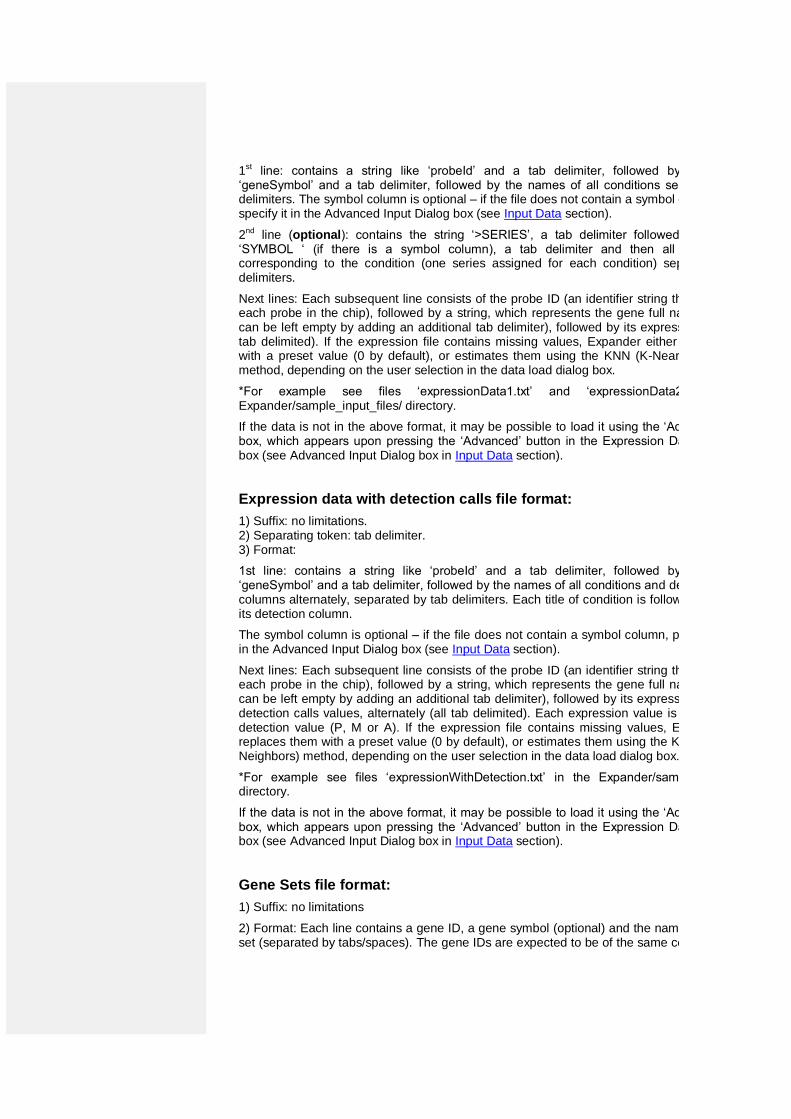
1st line: contains a string like ‘probeId’ and a tab delimiter, followed by a string like ‘geneSymbol’ and a tab delimiter, followed by the names of all conditions separated by tab delimiters. The symbol column is optional – if the file does not contain a symbol column, please specify it in the Advanced Input Dialog box (see Input Data section).
2nd line (optional): contains the string ‘>SERIES’, a tab delimiter followed by the string ‘SYMBOL ‘ (if there is a symbol column), a tab delimiter and then all series names corresponding to the condition (one series assigned for each condition) separated by tab delimiters.
Next lines: Each subsequent line consists of the probe ID (an identifier string that is unique to each probe in the chip), followed by a string, which represents the gene full name (if missing can be left empty by adding an additional tab delimiter), followed by its expression values (all tab delimited). If the expression file contains missing values, Expander either replaces them with a preset value (0 by default), or estimates them using the KNN (K-Nearest Neighbors) method, depending on the user selection in the data load dialog box.
*For example see files ‘expressionData1.txt’ and ‘expressionData2.txt’ in the Expander/sample_input_files/ directory.
If the data is not in the above format, it may be possible to load it using the ‘Advanced’ dialog box, which appears upon pressing the ‘Advanced’ button in the Expression Data load dialog box (see Advanced Input Dialog box in Input Data section).
Expression data with detection calls file format:
1) Suffix: no limitations. 2) Separating token: tab delimiter. 3) Format:
1st line: contains a string like ‘probeId’ and a tab delimiter, followed by a string like ‘geneSymbol’ and a tab delimiter, followed by the names of all conditions and detection signals columns alternately, separated by tab delimiters. Each title of condition is followed by a title of its detection column.
The symbol column is optional – if the file does not contain a symbol column, please specify it in the Advanced Input Dialog box (see Input Data section).
Next lines: Each subsequent line consists of the probe ID (an identifier string that is unique to each probe in the chip), followed by a string, which represents the gene full name (if missing can be left empty by adding an additional tab delimiter), followed by its expression values and detection calls values, alternately (all tab delimited). Each expression value is followed by its detection value (P, M or A). If the expression file contains missing values, Expander either replaces them with a preset value (0 by default), or estimates them using the KNN (K-Nearest Neighbors) method, depending on the user selection in the data load dialog box.
*For example see files ‘expressionWithDetection.txt’ in the Expander/sample_input_files/ directory.
If the data is not in the above format, it may be possible to load it using the ‘Advanced’ dialog box, which appears upon pressing the ‘Advanced’ button in the Expression Data load dialog box (see Advanced Input Dialog box in Input Data section).
Gene Sets file format:
1) Suffix: no limitations
2) Format: Each line contains a gene ID, a gene symbol (optional) and the name/number of its set (separated by tabs/spaces). The gene IDs are expected to be of the same convention used
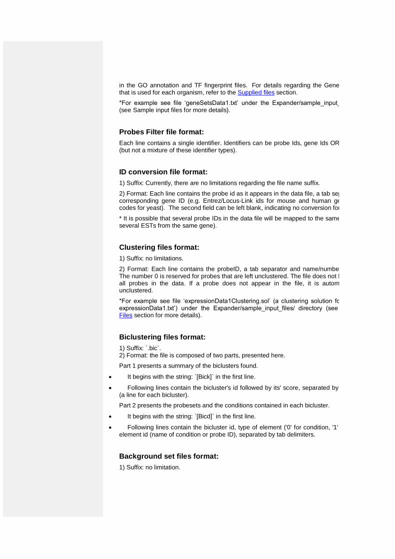
in the GO annotation and TF fingerprint files. For details regarding the Gene ID convention that is used for each organism, refer to the Supplied files section.
*For example see file ‘geneSetsData1.txt’ under the Expander/sample_input_files/ directory (see Sample input files for more details).
Probes Filter file format:
Each line contains a single identifier. Identifiers can be probe Ids, gene Ids OR gene symbols (but not a mixture of these identifier types).
ID conversion file format:
1) Suffix: Currently, there are no limitations regarding the file name suffix.
2) Format: Each line contains the probe id as it appears in the data file, a tab separator and the corresponding gene ID (e.g. Entrez/Locus-Link ids for mouse and human genes and ORF codes for yeast). The second field can be left blank, indicating no conversion for that probe ID.
* It is possible that several probe IDs in the data file will be mapped to the same gene ID (e.g.: several ESTs from the same gene).
Clustering files format:
1) Suffix: no limitations.
2) Format: Each line contains the probeID, a tab separator and name/number of its cluster. The number 0 is reserved for probes that are left unclustered. The file does not have to contain all probes in the data. If a probe does not appear in the file, it is automatically set as unclustered.
*For example see file ‘expressionData1Clustering.sol’ (a clustering solution for the data file’ expressionData1.txt’) under the Expander/sample_input_files/ directory (see Sample Input Files section for more details).
Biclustering files format:
1) Suffix: `.bic`. 2) Format: the file is composed of two parts, presented here.
Part 1 presents a summary of the biclusters found.
It begins with the string: `[Bick]` in the first line.
Following lines contain the bicluster's id followed by its' score, separated by a tab delimiter (a line for each bicluster).
Part 2 presents the probesets and the conditions contained in each bicluster.
It begins with the string: `[Bicd]` in the first line.
Following lines contain the bicluster id, type of element ('0' for condition, '1' for probe) and element id (name of condition or probe ID), separated by tab delimiters.
Background set files format:
1) Suffix: no limitation.
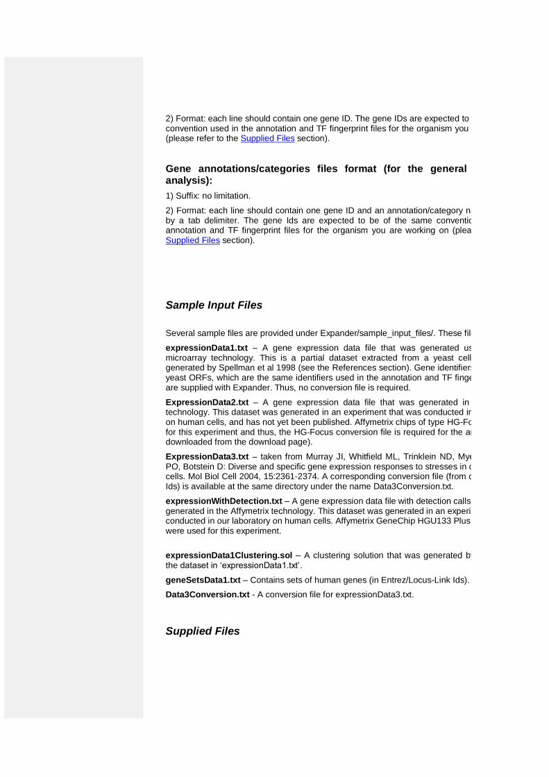
2) Format: each line should contain one gene ID. The gene IDs are expected to be of the same convention used in the annotation and TF fingerprint files for the organism you are working on (please refer to the Supplied Files section).
Gene annotations/categories files format (for the general enrichment analysis):
1) Suffix: no limitation.
2) Format: each line should contain one gene ID and an annotation/category name separated by a tab delimiter. The gene Ids are expected to be of the same convention used in the annotation and TF fingerprint files for the organism you are working on (please refer to the Supplied Files section).
Sample Input Files
Several sample files are provided under Expander/sample_input_files/. These files include:
expressionData1.txt – A gene expression data file that was generated using the cDNA microarray technology. This is a partial dataset extracted from a yeast cell cycle dataset generated by Spellman et al 1998 (see the References section). Gene identifiers in this set are yeast ORFs, which are the same identifiers used in the annotation and TF fingerprint files that are supplied with Expander. Thus, no conversion file is required.
ExpressionData2.txt – A gene expression data file that was generated in the Affymetrix technology. This dataset was generated in an experiment that was conducted in out laboratory on human cells, and has not yet been published. Affymetrix chips of type HG-Focus were used for this experiment and thus, the HG-Focus conversion file is required for the analysis (can be downloaded from the download page).
ExpressionData3.txt – taken from Murray JI, Whitfield ML, Trinklein ND, Myers RM, Brown PO, Botstein D: Diverse and specific gene expression responses to stresses in cultured human cells. Mol Biol Cell 2004, 15:2361-2374. A corresponding conversion file (from clone-Ids to LL-Ids) is available at the same directory under the name Data3Conversion.txt.
expressionWithDetection.txt – A gene expression data file with detection calls, that was generated in the Affymetrix technology. This dataset was generated in an experiment that was conducted in our laboratory on human cells. Affymetrix GeneChip HGU133 Plus 2.0 arrays were used for this experiment.
expressionData1Clustering.sol – A clustering solution that was generated by Expander for the dataset in ‘expressionData1.txt’.
geneSetsData1.txt – Contains sets of human genes (in Entrez/Locus-Link Ids).
Data3Conversion.txt - A conversion file for expressionData3.txt.
Supplied Files
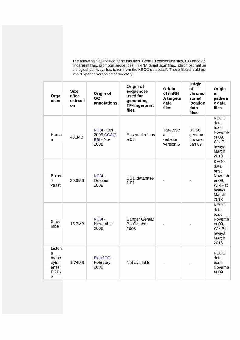
The following files include gene info files: Gene ID conversion files, GO annotation files, TF fingerprint files, promoter sequences, miRNA target scan files, chromosomal position files, and biological pathway files, taken from the KEGG database*. These files should be extracted
into "Expander/organisms" directory.
Organism
Size after extraction
Origin of GO annotations
Origin of sequences used for generating TF-fingerprint files
Origin of miRNA targets data files:
Origin of chromosomal location data files
Origin of pathway data files
Human
431MB
NCBI - Oct 2009,GOA@
EBI - Nov 2008
Ensembl release 53
TargetScan website version 5
UCSC genome browser Jan 09
KEGG data base November 09, WikiPathways March 2013
Baker's yeast
30.6MB NCBI - October 2009
SGD database 1.01
- -
KEGG data base November 09, WikiPathways March 2013
S. pombe
15.7MB
NCBI -
November 2008
Sanger GeneDB - October 2008
- -
KEGG data base November 09, WikiPathways March 2013
Listeria monocytosenes EGD-e
1.74MB
Blast2GO -
February 2009
Not available - -
KEGG data base November 09
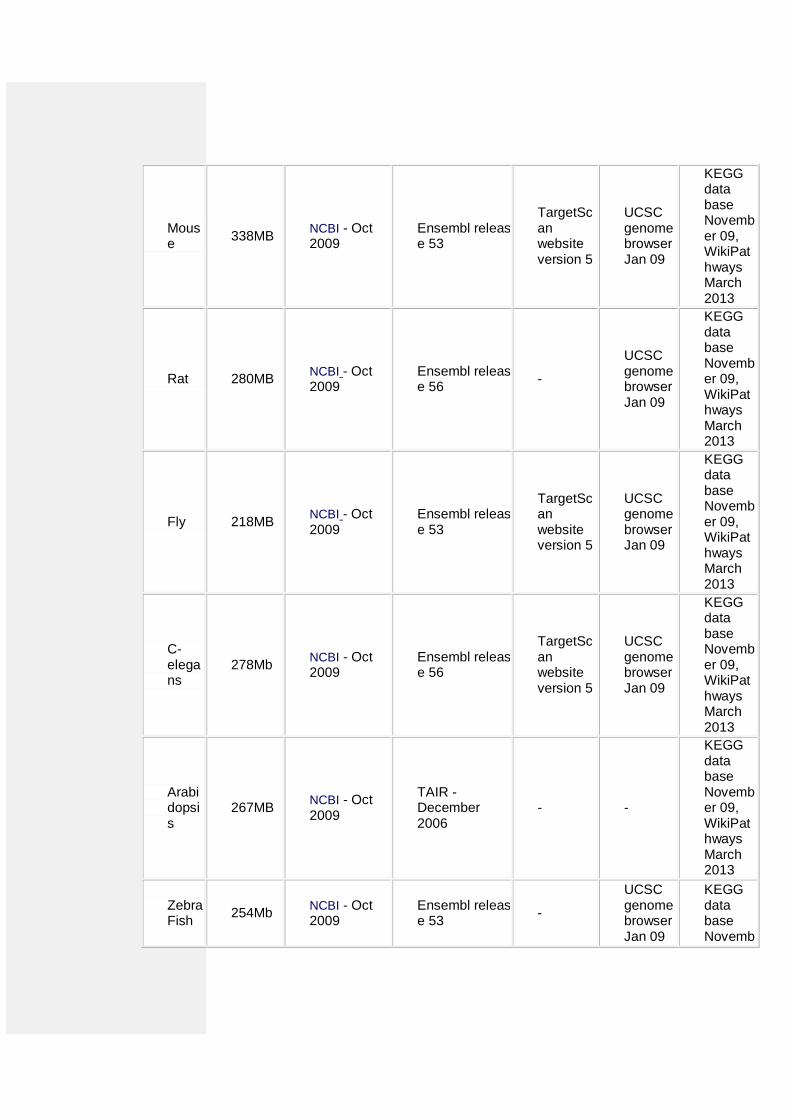
Mouse
338MB NCBI - Oct 2009
Ensembl release 53
TargetScan website version 5
UCSC genome browser Jan 09
KEGG data base November 09, WikiPathways March 2013
Rat 280MB NCBI - Oct 2009
Ensembl release 56
-
UCSC genome browser Jan 09
KEGG data base November 09, WikiPathways March 2013
Fly 218MB NCBI - Oct 2009
Ensembl release 53
TargetScan website version 5
UCSC genome browser Jan 09
KEGG data base November 09, WikiPathways March 2013
C-elegans
278Mb NCBI - Oct 2009
Ensembl release 56
TargetScan website version 5
UCSC genome browser Jan 09
KEGG data base November 09, WikiPathways March 2013
Arabidopsis
267MB NCBI - Oct 2009
TAIR - December 2006
- -
KEGG data base November 09, WikiPathways March 2013
Zebra Fish
254Mb NCBI - Oct 2009
Ensembl release 53
-
UCSC genome browser Jan 09
KEGG data base Novemb
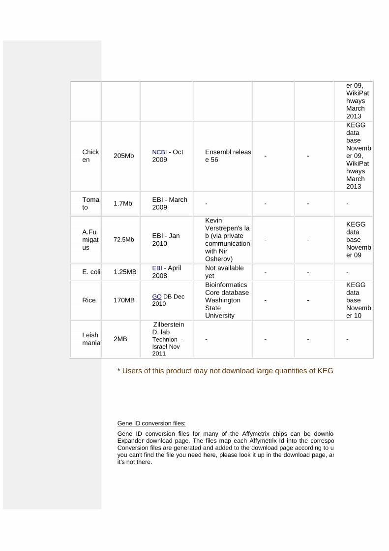
er 09, WikiPathways March 2013
Chicken
205Mb NCBI - Oct 2009
Ensembl release 56
- -
KEGG data base November 09, WikiPathways March 2013
Tomato
1.7Mb EBI - March 2009
- - - -
A.Fumigatus
72.5Mb EBI - Jan 2010
Kevin Verstrepen's lab (via private communication with Nir Osherov)
- -
KEGG data base November 09
E. coli 1.25MB EBI - April 2008
Not available yet
- - -
Rice 170MB GO DB Dec 2010
Bioinformatics Core database Washington State University
- -
KEGG data base November 10
Leishmania
2MB
Zilberstein D. lab Technion - Israel Nov 2011
- - - -
* Users of this product may not download large quantities of KEGG Data.
Gene ID conversion files:
Gene ID conversion files for many of the Affymetrix chips can be downloaded from the Expander download page. The files map each Affymetrix Id into the corresponding gene Id. Conversion files are generated and added to the download page according to user requests. If you can't find the file you need here, please look it up in the download page, and contact us if it's not there.
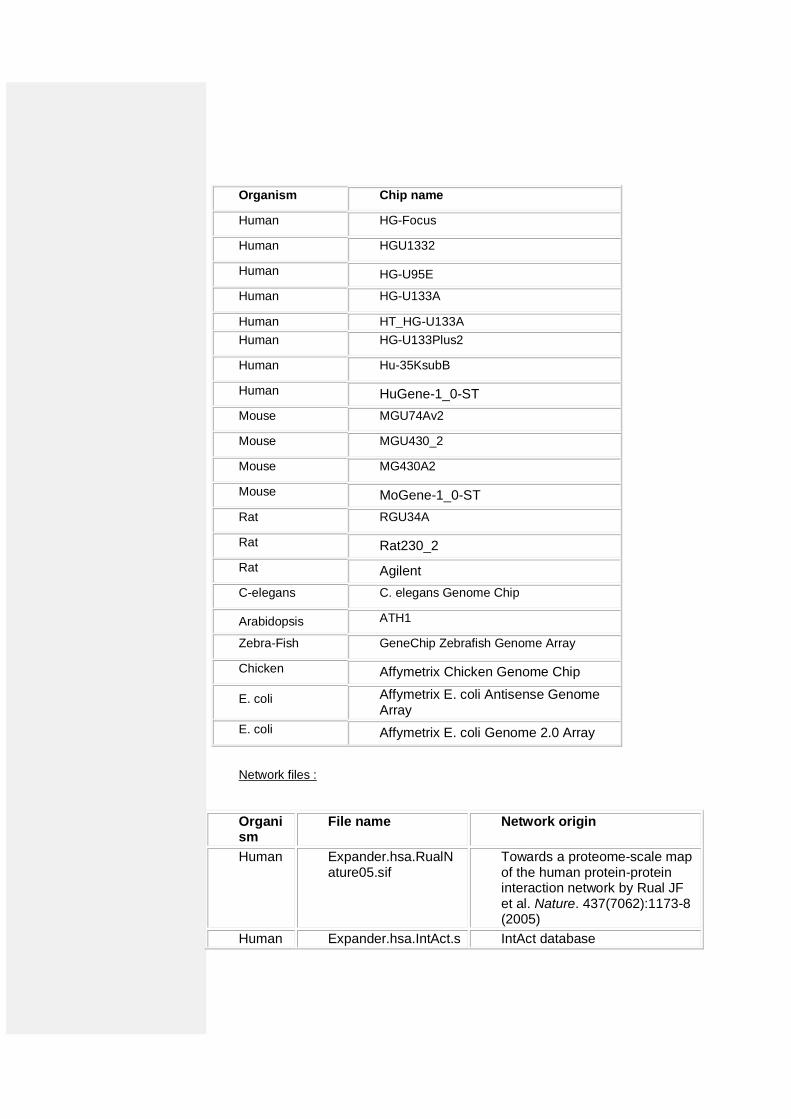
Organism Chip name
Human HG-Focus
Human HGU1332
Human HG-U95E
Human HG-U133A
Human HT_HG-U133A
Human HG-U133Plus2
Human Hu-35KsubB
Human HuGene-1_0-ST
Mouse MGU74Av2
Mouse MGU430_2
Mouse MG430A2
Mouse MoGene-1_0-ST
Rat RGU34A
Rat Rat230_2
Rat Agilent
C-elegans C. elegans Genome Chip
Arabidopsis ATH1
Zebra-Fish GeneChip Zebrafish Genome Array
Chicken Affymetrix Chicken Genome Chip
E. coli Affymetrix E. coli Antisense Genome Array
E. coli Affymetrix E. coli Genome 2.0 Array
Network files :
Organism
File name Network origin
Human Expander.hsa.RualNature05.sif
Towards a proteome-scale map of the human protein-protein interaction network by Rual JF et al. Nature. 437(7062):1173-8 (2005)
Human Expander.hsa.IntAct.s IntAct database
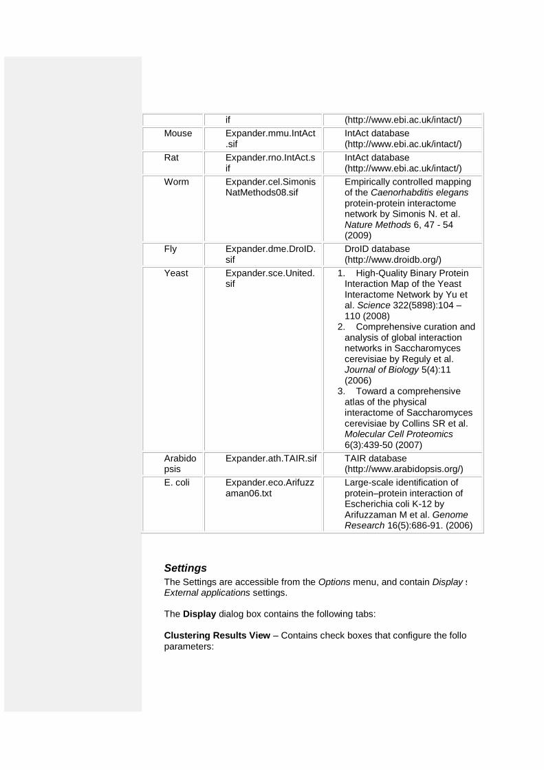
if (http://www.ebi.ac.uk/intact/)
Mouse Expander.mmu.IntAct.sif
IntAct database (http://www.ebi.ac.uk/intact/)
Rat Expander.rno.IntAct.sif
IntAct database (http://www.ebi.ac.uk/intact/)
Worm Expander.cel.SimonisNatMethods08.sif
Empirically controlled mapping of the Caenorhabditis elegans protein-protein interactome network by Simonis N. et al. Nature Methods 6, 47 - 54 (2009)
Fly Expander.dme.DroID.sif
DroID database (http://www.droidb.org/)
Yeast Expander.sce.United.sif
1. High-Quality Binary Protein Interaction Map of the Yeast Interactome Network by Yu et al. Science 322(5898):104 – 110 (2008)
2. Comprehensive curation and analysis of global interaction networks in Saccharomyces cerevisiae by Reguly et al. Journal of Biology 5(4):11 (2006)
3. Toward a comprehensive atlas of the physical interactome of Saccharomyces cerevisiae by Collins SR et al. Molecular Cell Proteomics 6(3):439-50 (2007)
Arabidopsis
Expander.ath.TAIR.sif TAIR database (http://www.arabidopsis.org/)
E. coli Expander.eco.Arifuzzaman06.txt
Large-scale identification of protein–protein interaction of Escherichia coli K-12 by Arifuzzaman M et al. Genome Research 16(5):686-91. (2006)
Settings
The Settings are accessible from the Options menu, and contain Display settings External applications settings. The Display dialog box contains the following tabs: Clustering Results View – Contains check boxes that configure the following
parameters:
A common Y-axis scale for all cluster patterns (vs. cluster specific)
Visible x axis
Connect all points in a pattern
Display similarity matrix for probes (using Pearson correlation)
Display similarity matrix for conditions (using Pearson correlation) Group Analysis Results View – Contains a check box that configures whether the Y-axis scale of all histograms is common OR cluster specific. Data Matrix View – Allows selection between:
Range control and extreme values control when rendering expression matrix values.
The red/green coloring scheme can be changed to blue/yellow. The External applications dialog box allows specification of the location of the R executable (required for CEL files loading). In Windows, R.exe file is likely to be located in the 'bin' folder of R software. In Linux, you may type 'which R' in the command line to find R path.
R External Application
The CEL file preprocessing and the newly added SAM filter utilities require the pre-installation of one of the recent versions of R, a free software environment for statistical computing and graphics. R can be installed from: http://cran.r-project.org/.
Upon the first time that Expander uses R external application, a window will pop, asking you to specify your R software location. Please browse to the location of your R software. In Windows, R.exe file is likely to be located in the 'bin' folder of R software. In Linux, you may type 'which R' in the command line to find R path. If you have a few versions of R installed, please make sure to point Expander to a version in which the necessary packages have been installed.
You may also specify R location from the menu: Options >> Settings >> External applications.
To use R utilities, please make sure there are no white spaces in the path of Expander directory (or the CEL files directory, if loading CEL files). For example, if the name of the Expander folder is 'Expander 5', change it to 'Expander_5'. If Expander is under "Program Files" it should be moved to another location, because of the space between "Program" and "Files". The R software does not cope well with spaces in the path. Also, please make sure to have 'write' permission to the Expander\Rscripts directory. If you are loading CEL files, check also that you have 'write' permission to the Files location which you specified in the 'Load CEL Files' dialog box.
After specifying R software location, a window will pop, asking you to approve or disapprove automatically installation of R packages when needed.
If you approve automatically installation of R packages then when R utility is used in Expander, Expander will automatically install the needed R packages for the used R utility.
If you disapprove automatically installation of R packages then please refer to "Manually installation of R packages" section.
Manually installation of R packages
After installing R, please do the following to install the Bioconductor “affy” package , "gcrma" package and the "samr" package:
1. Run R.
2. In the R frame\window type the text: source("http://bioconductor.org/biocLite.R")
3. Press ‘Enter’.
4. In the R frame\window type the text: biocLite("affy")
5. Press ‘Enter’.
To install the 'samr' package:
6. In the R frame\window type the text: install.packages("samr")
7. R frame\window type the text: install.packages("impute")
8. Press ‘Enter’.
To install the ‘eisa’ package:
9. In the R frame\window type the text: biocLite("eisa")
10. Press ‘Enter’.
To install the 'gcrma' package:
11. In the R frame\window type the text: source("http://bioconductor.org/biocLite.R")
12. Press ‘Enter’. In the R frame\window type the text:
13. biocLite("gcrma")
14. Press ‘Enter’.
You may install only one of the packages, depending on what you wish to use (to install only "samr", follow instructions number 1, 6 and 7).
FAQ
Linux/Unix problems
Click clustering, Samba bi-clustering, Tango and Prima Promoter analysis algorithms fail when running on Linux/Unix.
CEL Files Loading Problems
How do I install R and the Bioconductor "affy" package?
Loading of CEL files or performing SAM filter continue for ever
Loading of CEL files fail.
Clustering
When I try to run Biclustering on my data I get a failure notice.
How can I save the clustering expression patterns charts?
Grouping Analysis (functional and promoter analysis)
When I run Functional Analysis, Expander gets stuck.
When I load a session with that contains Functional Analysis results, Expander gets stuck,
When I try to run Promoter Analysis no values appear in the Fingerprints file field of the input dialog box.
When I try to run the promoter\functional analysis, I get a failure message box.
Promoter\Functional analysis produces no results (the resulting view is empty).
How can I save the bar charts produced by Expander, displaying the enrichments?
Why do certain Transcription Factors have a few accession numbers or\and a few gene IDs?
Saving sessions
When I try to save a session Expander fails and returns an XStream error message.
Others
Can I run Expander on Mac OS?
Click clustering, Samba bi-clustering, Tango and Prima Promoter analysis algorithms fail when running on Linux/Unix.
Answer: Make sure that you have write permission in the Expander directory, and execution permissions on the files: click.exe, samba.exe, annot_sets.exe and analyzeFingerprints.exe, which are under the Expander directory. If the problem still occurs, open the file expanderLog.txt and search for the text: “libstdc++.so.5”. If this text appears (along with a message indicating it has not been found), please contact your system administrator and report this problem (this is a system problem). If you do not have a system administrator, and fail to install this library, please contact us ([email protected]) and we will try to assist.
How do I install R and the Bioconductor "affy" package?
Answer: please refer to R External Application section.
Loading of CEL files or performing SAM filter continue forever.
Answer: If the operation continues forever (the 'processing, please wait' window is displayed), please check if there is a folder with a space in its name somewhere in the path of Expander (or the CEL files) directory. For example, if the name of the Expander folder is 'Expander 4', change it to 'Expander_4'. The R software used for preprocessing CEL files has a problem dealing with spaces in the path. If this is the problem, then in the expanderLog.txt file (in your Expander directory) there should be a message about arguments being ignored.
Loading of CEL files fail.
Answer: Make sure you have R along with the Bioconductor “affy” package installed in the R version which is specified in the settings “External Applications” tab (from the menu select Options >> Settings >> External applications). If R location is not defined in the settings, please define it (In Windows, R.exe file is likely to be located in the 'bin' folder of R software. In Linux, you may type 'which R' in the command line to find R path). If you are using an R package as cdf source, please make sure that the package is a folder located under your R library directory and that it is the correct package for your chip. If loading of CEL files still fails,
please make sure that the Files location which you specified in the 'Load CEL Files' dialog box, is a folder which contains CEL files and that you have write permission to that folder.
When I try to run Biclustering on my data I get a failure notice.
Answer: Make sure that the ‘Use option files of type’ field in the SAMBA input dialog box is not empty (if it is, please re-download Expander). Also make sure that the following files exist in your Expander directory: ibic.opt, samba.exe.
How can I save the clustering expression patterns charts?
When the clustering results tab is open, please go to File >> Save As Image.
When I run Functional Analysis, Expander gets stuck.
Answer: If you are working with Expander version 4.0 or 4.0.1, please update to a higher version (4.0.2 and on).
When I load a session with that contains Functional Analysis results, Expander gets stuck.
Answer: If you are working with Expander version 4.0 or 4.0.1 (and the session was created with a version < 4.0), please update to a higher version (4.0.2 and on).
When I try to run Promoter Analysis no values appear in the Fingerprints file field of the input dialog box.
Answer: Fingerprint files are not placed in the right directory. Fingerprint files should be placed under the ‘TF_fingerprints’ directory that is under the Expander/organism/<org name> directory. For example, the human FP file should be placed under: …/Expander/organisms/human/TF_fingerprints/. When downloading the organism specific data zip, it should be extracted into the Expander/organisms/ directory. This will automatically put them in the right place.
Group analysis (enrichment analysis) leads to a failure message box.
Answer: Errors while running group (enrichment) analysis can be caused by the following problems:
a) Organism specific data (Fingerprint\annotation files) is not in the right directory. The organism specific data zip should be extracted into the Expander/organisms/ directory. You may download the relevant data by selecting from the menu: Help >> Download Data for Organism.
b) Data contains elements that do not appear in the background set (this is only relevant when the background set is loaded from an external file).
Group analysis (enrichment analysis) produces no results (the resulting view is empty).
Answer: This can be caused by one of the following:
a) You are using the wrong conversion file or a conversion file that is not in the right format or does not map the probes to the expected type of gene Ids. The conversion file maps each probe ID in your data file to a gene ID that is used in the group analysis. A conversion file is

required when the probe Ids in your data file do not match the ones in the enrichment files (for example annotation and TF_fingerprint files that we supply).
b) You did not set the organism field in the input dialog to the organism type of your data.
c) You are trying to analyze only one set (e.g. the filtered data set) which you are using also as background (in this case the analysis has no meaning since it is trying to detect enrichments in the cluster/bicluster in comparison to the background set).
d) You set the threshold p-value to be too strict (low).
e) Biological reason i.e., there is nothing to report regarding this specific clustering/biclustering solution or this gene sets data.
How can I save the bar charts produced by Expander, displaying the enrichments?
When the results tab is open, please go to File >> Save As Image.
Why do certain Transcription Factors have a few accession numbers or\and a few gene IDs?
Answer: The transcription factors (TFs) found enriched by Prima are presented in the following way:
Accession Num. in TRANSFAC DB [TF name]. For example, M00287[NF-Y]
It is possible that a TF will have a few accession numbers in TRANSFAC, which represent different PWMs (position weight matrices specify the probability for observing each nucleotide at each position of the binding site, based on a set of empirically validated binding sites of the respective TF).
It is also possible that a TF will have a few Entrez gene IDs, since a TF may be composed of a few proteins. For example, NF-Y is a trimer, composed of 3 subunits.
Can I run Expander on Mac OS?
Expander is not designed for Mac OS. You can probably use it partially – without running its features that require the execution of exe files (CLICK, SAMBA, TANGO and PRIMA). The exe files are only suitable for Windows and Linux / Unix.
When I try to save a session, Expander fails and returns an XStream error message
If you are using java version 1.7, please switch to version 6. We currently have no solution for this problem, that occurs with java1.7 and XStream, which is an external package that we are using. We will do our best to resolve it in the coming future. In order to configure the Expander.bat files to use a java 6 version do the following:
1) Make sure that jave 6 (or 5) is installed on your PC by exploring the “Program Files (x86)/Java” (or “Program Files/Java”) directory. In it there should be a subdirectory by the name jre6 or jre5 (otherwise please install java6 from http://java.sun.com/javase/downloads/index.jsp.)
2) In the Expander directory right click on one of the Expander.bat files (the one you are using) and select “Edit”.
3) In the file type the path of the java6 exe file instead of the word java. E.g. if your path is C:\Program Files (x86)\Java\jre6 then put the text: “C:\Program Files (x86)\Java\jre6\bin\java.exe” (including the quotes (“”)) instead of the word java.
4) Remove the text “–client” from the file
5) Save and close the file
This section will be updated as we get user feedbacks and problems.
Please refer all questions/comments to [email protected].
Copyrights Information Copyrights © Tel-Aviv University, Israel (2003).
This product uses the FreeHEP Java Library, which is distributed under the LGPL license. FreeHEP copyright holders: CERN, Geneva, Switzerland SLAC, Stanford, California, U.S.A. University of California Santa Cruz, U.S.A.
This product uses the XStream Java Library, which is distributed under the BSD license (see BSD.txt). Copyright holders: (c) Joe Walnes 2003-2005 This product uses the Caryoscope java component, which is distributed under the MIT license (see MIT_Caryoscope.txt). Copyright holders: Copyright 2003-2004, Ihab A.B. Awad; Copyright 2006, Anjalee Sujanani; Stanford University. A portion of the user interface code is due to Sun Microsystems.Inc. Copyright 1994-2004 Sun Microsystems, Inc. All Rights Reserved. The following license rules apply to that portion:
‘Neither the name of Sun Microsystems, Inc. or the names of contributors may be used to endorse or promote products derived from this software without specific prior written permission.
This software is provided ‘AS IS,’ without a warranty of any kind. ALL EXPRESS OR IMPLIED CONDITIONS, REPRESENTATIONS AND WARRANTIES, INCLUDING ANY IMPLIED WARRANTY OF MERCHANTABILITY, FITNESS FOR A PARTICULAR PURPOSE OR NON-INFRINGEMENT, ARE HEREBY EXCLUDED. SUN MICROSYSTEMS, INC. (‘SUN’) AND ITS LICENSORS SHALL NOT BE LIABLE FOR ANY DAMAGES SUFFERED BY LICENSEE AS A RESULT OF USING, MODIFYING OR DISTRIBUTING THIS SOFTWARE OR ITS DERIVATIVES. IN NO EVENT WILL SUN OR ITS LICENSORS BE LIABLE FOR ANY LOST REVENUE, PROFIT OR DATA, OR FOR DIRECT, INDIRECT, SPECIAL, CONSEQUENTIAL, INCIDENTAL OR PUNITIVE DAMAGES, HOWEVER CAUSED AND REGARDLESS OF THE THEORY OF LIABILITY, ARISING OUT OF THE USE OF OR INABILITY TO USE THIS SOFTWARE, EVEN IF SUN HAS BEEN ADVISED OF THE POSSIBILITY OF SUCH DAMAGES.
You acknowledge that this software is not designed, licensed or intended for use in the design, construction, operation or maintenance of any nuclear facility.’
References R: R Development Core Team (2008). R: A language and environment for statistical computing. R Foundation for Statistical Computing, Vienna, Austria. ISBN 3-900051-07-0, URL http://www.R-project.org
affy package for CEL files preprocessing: Gautier, L., Cope, L., Bolstad, B. M., and Irizarry, R. A. 2004. affy---analysis of Affymetrix GeneChip data at the probe level. Bioinformatics 20, 3 (Feb. 2004), 307-315
gcrma R package: Jean(ZHIJIN) Wu and Rafael Irizarry with contributions from James MacDonald Jeff Gentry (). gcrma: Background Adjustment Using Sequence Information. R package version 2.14.1.
Quantile normalization: Bolstad, B. M. Irizarry, R. A. Astrand, M. and Speed, T. P. A Comparison of Normalization Methods for High Density Oligonucleotide Array Data Based on Variance and Bias. Bioinformatics 19(2):185-193, 2003
Non-linear baseline normalization: Schadt, E., C. Li, B. Eliss, and W. H. Wong. Feature extraction and normalization algorithms for high-density oligonucleotide gene expression array data. J. Cell. Biochem. 84(S37),120–125, 2002
SAM (Significance Analysis of Microarray):
V. Tusher., R. Tibshirani., and G. Chu. Significance analysis of microarrays applied to the ionizing radiation response. PNAS, 98: 5116-5121, 2001
R. Tibshirani, G. Chu, T. Hastie and Balasubramanian Narasimhan (). samr: SAM: Significance Analysis of Microarrays. R package version 1.26. http://www-stat.stanford.edu/~tibs/SAM
K-Means clustering algorithm: Tavazoie, S., Hughes, J. D., Campbell, M. J., Cho, R. J., and Church, G. M. Systematic determination of genetic network architecture. Nat Genet, 22: 281-285, 1999
SOM clustering algorithm: Tamayo, P., Slonim, D., Mesirov, J., Zhu, Q., Kitareewan, S., Dmitrovsky, E., Lander, E. S., and Golub, T. R. Interpreting patterns of gene expression with self-organizing maps: methods and application to hematopoietic differentiation. Proc Natl Acad Sci U S A, 96, 2907-2912, 1999
CLICK clustering algorithm: Sharan, R. and Shamir, R. CLICK: a clustering algorithm with applications to gene expression analysis. Proc Int Conf Intell Syst Mol Biol 8, 307-16, 2000
ISA Biclustering algorithm: Bergmann, S., Ihmels, J., Barkai, N. Iterative signature algorithm for the analysis of large-scale gene expression data. Phys Rev E Stat Nonlin Soft Matter Phys 2003 Mar; 67(3 Pt 1)
SAMBA biclustering algorithm: Tanay, A. Sharan, R. and Shamir, R. Discovering statistically significant biclusters in gene expression data. Bioinformatics, 18(1), 136-144, 2002
Matisse network grouping: Ulitsky, I. and Shamir, R. MATISSE: Identification of functional modules using network topology and high-throughput data. BMC Systems Biology, vol 1, No. 8 (2007)
Degas network grouping:
Ulitsky, I., Karp , R.M. and Shamir, R. Detecting Disease-Specific Dysregulated Pathways Via Analysis of Clinical Expression Profiles Proceedings of RECOMB 2008, pp. 347--359, LNBI 4955, Springer, Berlin, (2008). Context Scores for miRNA enrichment analysis: Grimson, A., Kai-How Farh, F. K
Johnston, W., Garrett-Engele, F., P Lim, L., P Bartel, D. MicroRNA Targeting Specificity in Mammals: Determinants beyond Seed Pairing. Molecular Cell, 27:91-105 (2007) PRIMA algorithm: Elkon, R., Linhart, C. Sharan, R. Samir, R. and Shiloh, Y. Genome-Wide In Silico Identification of Transcriptional Regulators Controlling the Cell Cycle in Human Cells. Genome Research, Vol. 13(5), pp. 773-780, 2003.
Spike software and DB: R. Elkon, R. Vesterman, N. Amit, I. Ulitsky, I. Zohar, M. Weisz, G. Mass, N. Orlev, G. Sternberg, R. Blekhman, J. Assa, Y. Shiloh and R.Shamir. SPIKE - a database, visualization and analysis tool of cellular signaling pathways. BMC Bioinformatics 2008, 9:11
Spike home page: http://www.cs.tau.ac.il/~spike/
Agglomerative algorithm for hierarchical clustering: Eisen, M. B., Spellman, P. T. et al. Cluster analysis and display of genome-wide expression patterns. Proc Natl Acad Sci U S A 95(25), 14863-8, 1998
TF binding site profiles that were used to generate the supplied yeast TF fingerprint files: Harbison, C.T., D.B. Gordon, T.I. Lee, N.J. Rinaldi, K.D. Macisaac, T.W. Danford, N.M. Hannett, J.B. Tagne, D.B. Reynolds, J. Yoo, E.G. Jennings, J. Zeitlinger, D.K. Pokholok, M. Kellis, P.A. Rolfe, K.T. Takusagawa, E.S. Lander, D.K. Gifford, E. Fraenkel, and R.A. Young. Transcriptional regulatory code of a eukaryotic genome. Nature 431: 99-104, 2004
expressionData1.txt sample input file: Spellman, P. T., Sherlock, G., et al. Comprehensive identification of cell cycle-regulated genes of the yeast Saccharomyces cerevisiae by microarray hybridization. Mol Biol Cell 9(12), 3273-97, 1998
Gene Set Enrichment Analysis: Aravind Subramanian, Pablo Tamayo, Vamsi K. Mootha, Sayan Mukherjee, Benjamin L. Ebert, Michael A. Gillette, Amanda Paulovich, Scott L. Pomeroy, Todd R. Golub, Eric S. Lander, and Jill P. Mesirov. Gene set enrichment analysis: A knowledge-based approach for interpreting genome-wide expression profiles. PNAS vol. 102, no. 43, 15545–15550, 2005