Operation Control Protocols in Power Distribution Grids∗

Yehia Abd Alrahman†1,2 and Hugo Torres Vieira‡1

1IMT School for Advanced Studies, Lucca, Italy2University of Leicester, Leicester, UK

Abstract

Future power distribution grids will comprise a large number of components, each potentially ableto carry out operations autonomously. Clearly, in order to ensure safe operation of the grid, individualoperations must be coordinated among the different components. Since operation safety is a globalproperty, modelling component coordination typically involves reasoning about systems at a global level.In this paper, we propose a language for specifying grid operation control protocols from a global point ofview. We show how such global specifications can be used to automatically generate local controllers ofindividual components, and that the distributed implementation yielded by such controllers operationallycorresponds to the global specification. We showcase our development by modelling a fault managementscenario in power grids.

Keywords: Power Grids, Interaction Protocols, Process Calculus

1 Introduction

Modern power grids are large systems comprising a large number of geographically dispersed components.For example, the transmission lines of the North American power grid link all electricity generation anddistribution in the continent [5]. Because such grids are highly interconnected, any failure even in one locationmight be magnified as it propagates through the grid’s infrastructure to cause instantaneous impacts on awide area, causing what is called Cascading effects [12]. This means that power grids might exhibit a globalfailure almost instantaneously as a result of a local one. It is therefore crucial that future power grids areequipped with mechanisms that enable self-healing, and support automatic power restoration, voltage control,and power flow management.

Current power grids suffer from the fact that control operations and power flow management are doneby relying on a central control through the supervisory control and data acquisition (SCADA) system [20].Although the operational principles of interconnected power grids have been established ever since the 1960s,the coordination of control operations across the infrastructure of a power grid has received less attention [5].This is due to the fact that the operational principles were established before the emergence of powerfulcomputers and communication networks. Computation is now largely used in all levels of the power grid,but coordination happens on a slower rate. Actually, only specific coordination operations are carried outby computer control while the rest is still based on telephone calls between system operators at the utilitycontrol centres even during emergencies. Furthermore, protection systems are limited to manage specificinfrastructure components only.

Clearly, the current centralised control and protection systems cannot cope with the level of dynamicityand demands of modern power grids. Future power grids should be both flexible and extensible. Flexibilityin the sense of their ability to reconfigure and adapt in response to failures. Extensible in the sense that newcomponents can be added or removed from the grid without compromising its overall operation. Such type of

∗Yehia Abd Alrahman has been partially funded by the ERC consolidator grant DSynMA under the European UnionsHorizon 2020 research and innovation programme (grant agreement No 772459).†yehia.abdalrahman@leicester.ac.uk‡hugotvieira@imtlucca.it

1

arX

iv:1

811.

0194

2v1

[cs

.LO

] 5

Nov

201

8

grids would ease the integration of distributed generation (DG) (e.g., using renewable energy) and energystorage. A promising idea is to allow distributed control instead of the centralised one, as proposed by theEuropean SmartGrids Technology Platform [2] and the IntelliGrid project [1].

The idea is to view the power grid as a collection of independent and autonomous substations, collaboratingto achieve a desired global goal. It is then necessary to equip each substation with an independent controllerthat is able to communicate and cooperate with others, forming a large distributed computing system. Eachcontroller must be connected to sensors associated with its own substation so that it can assess its own statusand report them to its neighbouring controllers via communication paths. The communication paths of thecontrollers should follow the electrical connection paths. In this way, each substation can have a local view ofthe grid, represented by the connections to its neighbours.

Despite the many advances of tools [16, 13, 9], theoretical foundation to fully design and manage powersystems is still lacking [6]. In this paper, we propose a formal model of distributed power systems (Sect. 2),and we show how automatic synthesis of substation controllers can be obtained (Sect. 3). More precisely, weprovide a compact high-level language that can be used to specify the operation control protocols governingthe actual behaviour of the whole power grid from a global point of view. Also, we show how our globalmodel can be used to automatically synthesise individual controllers that yield a distributed implementation.To showcase our development we model a fault management scenario (Sect. 4).

The main advantage of our approach is that it reduces the engineering complexity of power grids bymeans of decentralising decision making among substations. Thus, power grid management is carried outlocally, avoiding overloading the control centre both at the level of the communication infrastructure and ofoperation control. Furthermore, the global model is more amenable to verify (global) system-level properties.Thanks to an operational correspondence result between the global model and the automatically generateddistributed model, we can also ensure that any property that holds for the global specification also holds forthe distributed implementation.

In what follows, we informally present the language that supports the specification of operation controlprotocols from a global perspective, i.e., considering the set of interactions as a whole. For the sake of a moreintuitive reading, we introduce and motivate our design choices by pointing to the fault management scenariowhich will be fully explained in Sect. 4. In Sect. 2 and Sect. 3, we present the syntax and the semantics ofthe global and the distributed language respectively. In Sect. 3, we also show how to automatically synthesisethe operationally precise behaviour of individual substations given the global specification of the protocol. InSect. 4, we show how natural and intuitive it is to program a sizeable and interesting case study from therealm of power grids using the global syntax and we then show how the synthesis works. Finally, in Sect. 5,we comment on research directions and present related work.

1.1 Operation Control Protocols, Informally

We consider a scenario involving a power distribution grid where a fault occurs in one of the transmissionpower lines, and a recovery protocol that locates and isolates the fault by means of interactions among thenodes in the grid.

A central notion in our proposal is that nodes involved in such a protocol yield control by means ofsynchronisation actions. For example, consider a node that is willing to Locate the fault and another onethat can react and continue the task of locating the fault. The two nodes may synchronise on action Locateand the enabling node yields the control to the reacting one. We therefore consider that active nodes enablesynchronisations and, as a consequence of a synchronisation, transfer the active role to the reacting node. So,for example, after some node 1 synchronises with some node 2 on Locate, node 2 may enable the followinginteraction, e.g., a synchronisation with some node 3 also on Locate.

We may therefore specify protocols as a (structured) set of interactions without identifying the actualnodes involved a priori, since these are determined operationally due to the transference of the active rolein synchronisations. We write [Locate ] P to specify a protocol stating that a synchronisation on Locateis to take place first, after which the protocol proceeds as specified by P (for now we abstract from theremaining elements using ). Also, we write (1)P ′ to specify that node 1 is active on protocol P ′. So, by(1)[Locate ] P we represent that node 1 may enable the synchronisation on Locate. Furthermore, we maywrite (1)[Locate ] P −→ [Locate ] (2)P to represent such a synchronisation step (−→) between nodes 1 and 2,where node 1 yields the control and node 2 is activated to carry out the continuation protocol P . This allows

2

to capture the transference of the active role in the different stages of the protocol.Interaction in our model is driven by the network communication topology that accounts for radial power

supply configurations (i.e, tree-like structures where root nodes provide power to the respective subtrees),and for a notion of proximity (so as to capture, e.g., backup links and address network reconfigurations). Wetherefore consider that nodes can interact if they are in a provide/receive power relation or in a neighbouringrelation. To this end, synchronisation specifications include a direction to determine the target of thesynchronisation. For example, by [Locate?] we represent that Locate targets all (child) nodes (?) that receivepower from the enabling node, used in the scenario by the root(s) to search for the fault in the power supply(sub)tree. Also, by [RecoverN] we specify that Recover targets the power provider (N) of the enabling node(i.e., the parent node), used in the scenario to signal when the fault has been found. Finally, by [PowerI] werepresent that Power targets a neighbouring node (I), used in the scenario for capturing power restorationand associated network reconfiguration.

Combining two of the above example synchronisations by means of recursion and summation (+), we maythen write a simplified fault management protocol

Simple , rec X.([Locate?]c1c1∨c2X + [RecoverN]c2tt 0) (1)

which specifies an alternative between Locate and Recover synchronisations, where in the former case theprotocol starts over and in the latter case terminates. Also, to support a more fine grained description ofprotocols, the synchronisation actions specify conditions (omitted previously with ) that must hold for bothenabling and reacting nodes in order for a synchronisation to take place. For example, only nodes that areat the root of a (sub)tree that has a fault may enable a synchronisation on Locate, which is captured incondition c1 (left unspecified here). Also, only nodes that satisfy such condition (c1) or that are withoutpower supply (which is captured in condition c2) can react to Locate. For Recover, the specification says thatonly nodes that are without power supply (c2) can enable the synchronisation, while any node can react to it(captured by condition true tt). The general idea is that the Locate synchronisations propagate throughoutthe power supply tree, one level per synchronisation, up to the point the fault is located and synchronisationRecover leads to termination.

The combination of the summation and of synchronisation conditions thus allows for a fine-grainedspecification of the operation control protocol. Furthermore, the conditions specified for synchronisationsare checked against the state of nodes, so state information is accounted for in our model. To represent thedynamics of systems, such state may evolve throughout the stages of the operation protocol. We thereforeconsider that synchronisation actions may have side-effects on the state of the nodes that synchronise. Thisallows to avoid introducing specialised primitives and simplifies reasoning on protocols, given the atomicity ofthe synchronisation and side-effect in one step.

The general principles described above, identified in the context of a fault management scenario, guidedthe design of the language presented in the next section. Although this is not the case for a single fault, weremark that our language addresses scenarios where several nodes may be active simultaneously in possiblydifferent stages of the protocol. A detailed account of the fault management scenario is presented in Sect. 4,including a protocol designed to account for configurations with several faults.

2 A Model for Operation Control Protocols

The syntax of the language is given in Table 1, where we assume a set of node identifiers (id , . . .), synchronisa-tion action labels (f, . . .), and logical conditions (c, i, o, . . .). Protocols (P,Q, . . .) combine static specificationsand the active node construct. The latter is denoted by (id)P , representing that node id is active to carry outthe protocol P . Static specifications include termination 0, fork P |Q which says that both P and Q are to becarried out, and infinite behaviour defined in terms of the recursion rec X.P and recursion variable X, withthe usual meaning. Finally, static specifications include synchronisation summations (S, . . .), where S1 + S2

says that either S1 is to be carried out or S2 (exclusively), and where [fd]oiP represents a synchronisationaction: a node active on [fd]oiP that satisfies condition o may synchronise on f with the node(s) identifiedby the direction d for which condition i holds, leading to the activation of the latter node(s) on protocolP . Intuitively, the node active on [fd]oiP enables the synchronisation, which results in the reaction of thetargeted nodes that are activated to carry out the continuation protocol P .

3

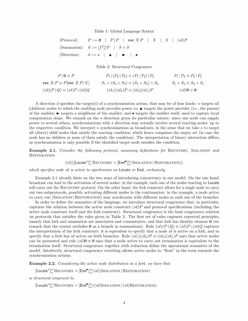
Table 1: Global Language Syntax

(Protocol) P ::= 0 | P |P | rec X.P | X | S | (id)P

(Summation) S ::= [fd]oiP | S + S

(Direction) d ::= ? | N | I | •

Table 2: Structural Congruence

P |0 ≡ P P1 | (P2 |P3) ≡ (P1 |P2) |P3 P1 |P2 ≡ P2 |P1

rec X.P ≡ P [rec X.P/X] S1 + (S2 + S3) ≡ (S1 + S2) + S3 S1 + S2 ≡ S2 + S1

(id)(P |Q) ≡ (id)P | (id)Q (id1)(id2)P ≡ (id2)(id1)P (id)0 ≡ 0

A direction d specifies the target(s) of a synchronisation action, that may be of four kinds: ? targets all(children) nodes to which the enabling node provides power to; N targets the power provider (i.e., the parent)of the enabler; I targets a neighbour of the enabler; and • targets the enabler itself, used to capture localcomputation steps. We remark on the ? direction given its particular nature: since one node can supplypower to several others, synchronisations with ? direction may actually involve several reacting nodes, up tothe respective condition. We interpret ? synchronisations as broadcasts, in the sense that we take ? to targetall (direct) child nodes that satisfy the reacting condition, which hence comprises the empty set (in case thenode has no children or none of them satisfy the condition). The interpretation of binary interaction differs,as synchronisation is only possible if the identified target node satisfies the condition.

Example 2.1. Consider the following protocol, assuming definitions for Recovery, Isolation andRestoration

(id)([Locate?]o1i1 Recovery + [End•]o2i2 (Isolation |Restoration))

which specifies node id is active to synchronise on Locate or End, exclusively.

Example 2.1 already hints on the two ways of introducing concurrency in our model. On the one hand,broadcast can lead to the activation of several nodes: in the example, each one of the nodes reacting to Locatewill carry out the Recovery protocol. On the other hand, the fork construct allows for a single node to carryout two subprotocols, possibly activating different nodes in the continuation: in the example, a node activeto carry out (Isolation |Restoration) may synchronise with different nodes in each one of the branches.

In order to define the semantics of the language, we introduce structural congruence that, in particular,captures the relation between the active node construct (id)P and protocol specifications (including theactive node construct itself and the fork construct). Structural congruence is the least congruence relationon protocols that satisfies the rules given in Table 2. The first set of rules captures expected principles,namely that fork and summation are associative and commutative, and that fork has identity element 0 (weremark that the syntax excludes 0 as a branch in summations). Rule (id)(P |Q) ≡ (id)P | (id)Q capturesthe interpretation of the fork construct: it is equivalent to specify that a node id is active on a fork, and tospecify that a fork has id active on both branches. Rule (id1)(id2)P ≡ (id2)(id1)P says that active nodescan be permuted and rule (id)0 ≡ 0 says that a node active to carry out termination is equivalent to thetermination itself. Structural congruence together with reduction define the operational semantics of themodel. Intuitively, structural congruence rewriting allows active nodes to “float” in the term towards thesynchronisation actions.

Example 2.2. Considering the active node distribution in a fork, we have that

[Locate?]o1i1 Recovery + [End•]o2i2 (id)(Isolation |Restoration)

is structural congruent to

[Locate?]o1i1 Recovery + [End•]o2i2 ((id)Isolation | (id)Restoration)

4

The definition of reduction depends on the network topology and on the fact that nodes satisfy certainlogical conditions. We consider state information for each node so as to capture both “local” information aboutthe topology (such as the identities of the power provider and of the set of neighbours) and other informationrelevant for condition assessment (such as the status of the power supply). The network state, denoted by∆, is a mapping from node identifiers to states, where a state, denoted by s, is a register id [id ′, t, n, k, a, e]containing the following information: id is the node identifier; id ′ identifies the power provider; t capturesthe status of the input power connection; n is the set of identifiers of neighbouring nodes; k is the powersupply capacity of the node; a is the number of active power supply links (i.e., the number of nodes thatreceive power from this one); and e is the number of power supply links that are in a faulty state.

As mentioned in Section 1.1, we check conditions against states for the purpose of allowing synchronisations.Given a state s we denote by s |= c that state s satisfies condition c, where we leave the underlying logicunspecified. For example, we may say that s |= (k > 0) to check that s has capacity greater than 0.

Also mentioned in Section 1.1 is the notion of side-effects, in the sense that synchronisation actions mayresult in state changes so as to model system evolution. By upd(id , id ′, fd,∆) we denote the operation thatyields the network state obtained by updating ∆ considering node id synchronises on f with id ′, hence theupdate regards the side-effects of f in the involved nodes. Namely, given ∆ = (∆′, id 7→ s, id ′ 7→ s′) we havethat upd(id , id ′, fd,∆) is defined as (∆′, id 7→ fd!(s, id ′), id ′ 7→ fd?(s′, id)), where fd!(s, id ′) modifies state saccording to the side-effects of enabling fd and considering id ′ is the reactive node (likewise for the reactingupdate, distinguished by ?). We consider side-effects only for binary synchronisations (I and N directions),but state changes could also be considered for other directions in similar lines.

The definition of reduction relies on an auxiliary operation, denoted d(∆, id), that yields the recipient(s)of a synchronisation action, given the direction d, the network state ∆, and the enabler of the action id . Theoperation, defined as follows, thus yields the power provider of the node in case the direction is N, (any) oneof the neighbours in case the direction is I, all the nodes that have as parent the enabler in case the directionis ?, and is undefined for direction •.

N(∆, id) , id ′ (if ∆(id) = id [id ′, t, n, k, a, e])

I (∆, id) , id ′ (if ∆(id) = id [id ′′, t, n, k, a, e] and id ′ ∈ n)

?(∆, id) , {id ′ | N(∆, id ′) = id}•(∆, id) , undefined

The reduction relation is given in terms of configurations consisting of a protocol P and a mapping ∆,for which we use ∆;P to denote the combination. By ∆;P −→ ∆′;P ′ we represent that configuration ∆;Pevolves in one step to configuration ∆′;P ′, potentially involving state changes (∆ and ∆′ may differ) and(necessarily) involving a step in the protocol from P to P ′.

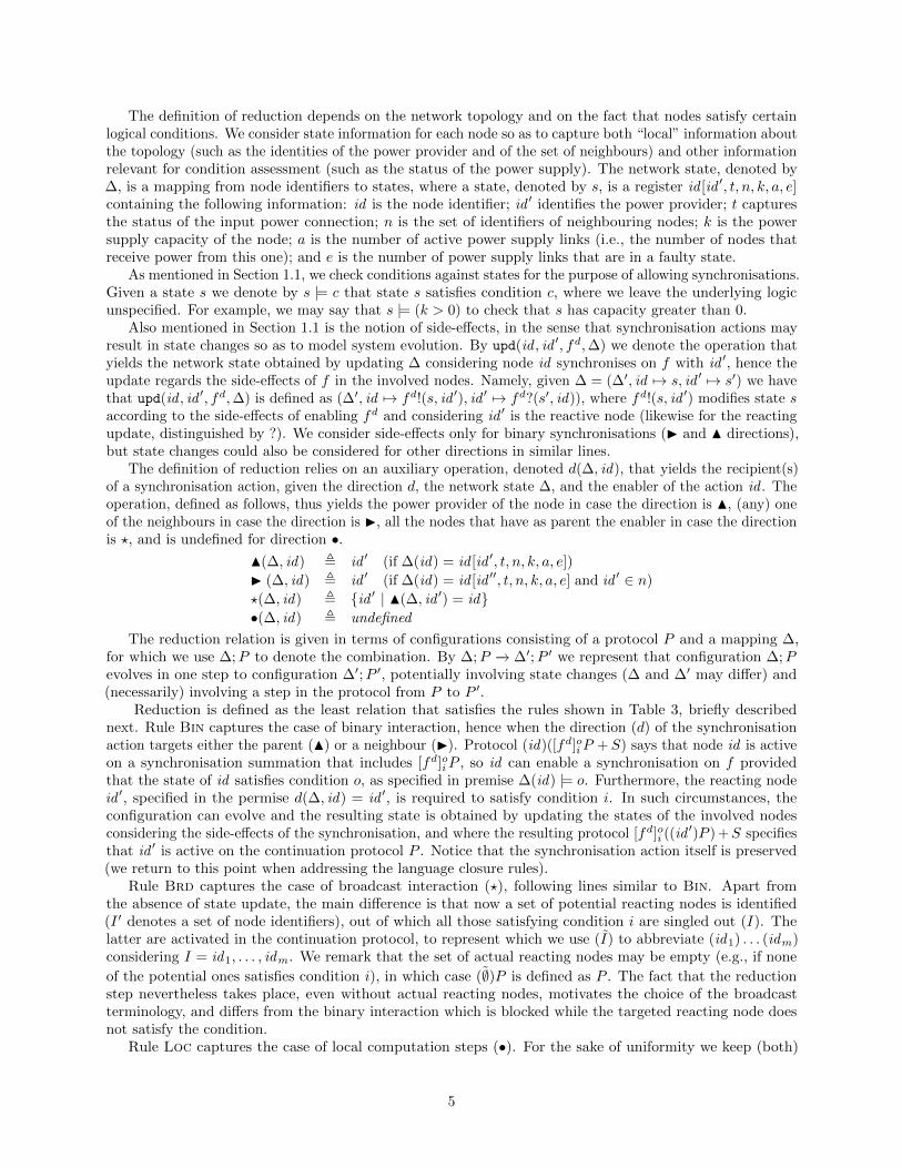
Reduction is defined as the least relation that satisfies the rules shown in Table 3, briefly describednext. Rule Bin captures the case of binary interaction, hence when the direction (d) of the synchronisationaction targets either the parent (N) or a neighbour (I). Protocol (id)([fd]oiP + S) says that node id is activeon a synchronisation summation that includes [fd]oiP , so id can enable a synchronisation on f providedthat the state of id satisfies condition o, as specified in premise ∆(id) |= o. Furthermore, the reacting nodeid ′, specified in the permise d(∆, id) = id ′, is required to satisfy condition i. In such circumstances, theconfiguration can evolve and the resulting state is obtained by updating the states of the involved nodesconsidering the side-effects of the synchronisation, and where the resulting protocol [fd]oi ((id

′)P ) +S specifiesthat id ′ is active on the continuation protocol P . Notice that the synchronisation action itself is preserved(we return to this point when addressing the language closure rules).

Rule Brd captures the case of broadcast interaction (?), following lines similar to Bin. Apart fromthe absence of state update, the main difference is that now a set of potential reacting nodes is identified(I ′ denotes a set of node identifiers), out of which all those satisfying condition i are singled out (I). Thelatter are activated in the continuation protocol, to represent which we use (I) to abbreviate (id1) . . . (idm)considering I = id1, . . . , idm. We remark that the set of actual reacting nodes may be empty (e.g., if none

of the potential ones satisfies condition i), in which case (∅)P is defined as P . The fact that the reductionstep nevertheless takes place, even without actual reacting nodes, motivates the choice of the broadcastterminology, and differs from the binary interaction which is blocked while the targeted reacting node doesnot satisfy the condition.

Rule Loc captures the case of local computation steps (•). For the sake of uniformity we keep (both)

5

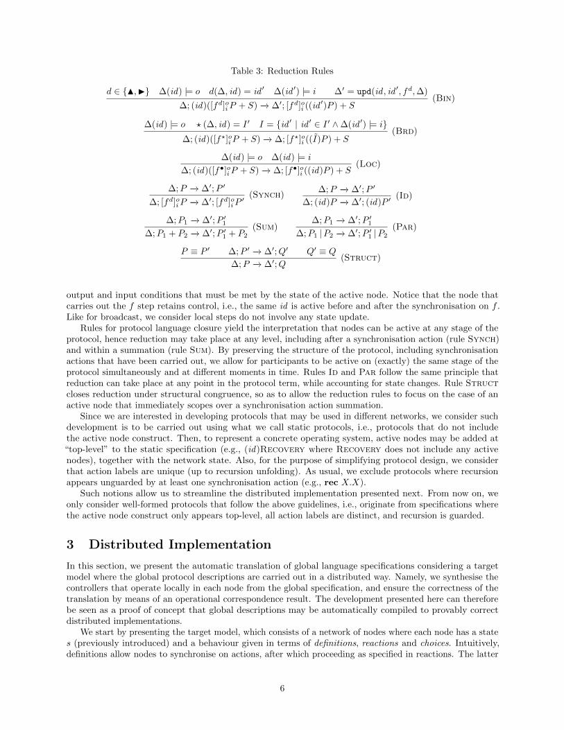
Table 3: Reduction Rules

d ∈ {N,I} ∆(id) |= o d(∆, id) = id ′ ∆(id ′) |= i ∆′ = upd(id , id ′, fd,∆)

∆; (id)([fd]oiP + S) −→ ∆′; [fd]oi ((id′)P ) + S

(Bin)

∆(id) |= o ? (∆, id) = I ′ I = {id ′ | id ′ ∈ I ′ ∧∆(id ′) |= i}∆; (id)([f?]oiP + S) −→ ∆; [f?]oi ((I)P ) + S

(Brd)

∆(id) |= o ∆(id) |= i

∆; (id)([f•]oiP + S) −→ ∆; [f•]oi ((id)P ) + S(Loc)

∆;P −→ ∆′;P ′

∆; [fd]oiP −→ ∆′; [fd]oiP′ (Synch)

∆;P −→ ∆′;P ′

∆; (id)P −→ ∆′; (id)P ′(Id)

∆;P1 −→ ∆′;P ′1∆;P1 + P2 −→ ∆′;P ′1 + P2

(Sum)∆;P1 −→ ∆′;P ′1

∆;P1 |P2 −→ ∆′;P ′1 |P2(Par)

P ≡ P ′ ∆;P ′ −→ ∆′;Q′ Q′ ≡ Q∆;P −→ ∆′;Q

(Struct)

output and input conditions that must be met by the state of the active node. Notice that the node thatcarries out the f step retains control, i.e., the same id is active before and after the synchronisation on f .Like for broadcast, we consider local steps do not involve any state update.

Rules for protocol language closure yield the interpretation that nodes can be active at any stage of theprotocol, hence reduction may take place at any level, including after a synchronisation action (rule Synch)and within a summation (rule Sum). By preserving the structure of the protocol, including synchronisationactions that have been carried out, we allow for participants to be active on (exactly) the same stage of theprotocol simultaneously and at different moments in time. Rules Id and Par follow the same principle thatreduction can take place at any point in the protocol term, while accounting for state changes. Rule Structcloses reduction under structural congruence, so as to allow the reduction rules to focus on the case of anactive node that immediately scopes over a synchronisation action summation.

Since we are interested in developing protocols that may be used in different networks, we consider suchdevelopment is to be carried out using what we call static protocols, i.e., protocols that do not includethe active node construct. Then, to represent a concrete operating system, active nodes may be added at“top-level” to the static specification (e.g., (id)Recovery where Recovery does not include any activenodes), together with the network state. Also, for the purpose of simplifying protocol design, we considerthat action labels are unique (up to recursion unfolding). As usual, we exclude protocols where recursionappears unguarded by at least one synchronisation action (e.g., rec X.X).

Such notions allow us to streamline the distributed implementation presented next. From now on, weonly consider well-formed protocols that follow the above guidelines, i.e., originate from specifications wherethe active node construct only appears top-level, all action labels are distinct, and recursion is guarded.

3 Distributed Implementation

In this section, we present the automatic translation of global language specifications considering a targetmodel where the global protocol descriptions are carried out in a distributed way. Namely, we synthesise thecontrollers that operate locally in each node from the global specification, and ensure the correctness of thetranslation by means of an operational correspondence result. The development presented here can thereforebe seen as a proof of concept that global descriptions may be automatically compiled to provably correctdistributed implementations.

We start by presenting the target model, which consists of a network of nodes where each node has a states (previously introduced) and a behaviour given in terms of definitions, reactions and choices. Intuitively,definitions allow nodes to synchronise on actions, after which proceeding as specified in reactions. The latter

6

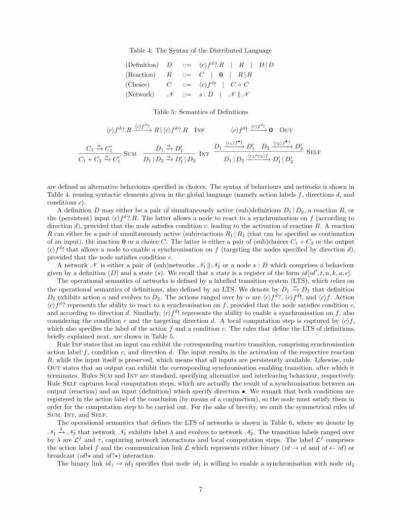
Table 4: The Syntax of the Distributed Language

(Definition) D ::= 〈c〉fd?.R | R | D |D(Reaction) R ::= C | 0 | R |R(Choice) C ::= 〈c〉fd! | C + C

(Network) N ::= s : D | N ‖N

Table 5: Semantics of Definitions

〈c〉fd?.R 〈c〉fd?−−−−→ R | 〈c〉fd?.R Inp 〈c〉fd! 〈c〉fd!−−−−→ 0 Out

C1α−→ C ′1

C1 + C2α−→ C ′1

SumD1

α−→ D′1

D1 |D2α−→ D′1 |D2

IntD1

〈c1〉f•!−−−−→ D′1 D2〈c2〉f•?−−−−−→ D′2

D1 |D2〈c1∧c2〉f−−−−−−→ D′1 |D′2

Self

are defined as alternative behaviours specified in choices. The syntax of behaviours and networks is shown inTable 4, reusing syntactic elements given in the global language (namely action labels f , directions d, andconditions c).

A definition D may either be a pair of simultaneously active (sub)definitions D1 |D2, a reaction R, orthe (persistent) input 〈c〉fd?.R. The latter allows a node to react to a synchronisation on f (according todirection d), provided that the node satisfies condition c, leading to the activation of reaction R. A reactionR can either be a pair of simultaneously active (sub)reactions R1 |R2 (that can be specified as continuationof an input), the inaction 0 or a choice C. The latter is either a pair of (sub)choices C1 + C2 or the output〈c〉fd! that allows a node to enable a synchronisation on f (targeting the nodes specified by direction d),provided that the node satisfies condition c.

A network N is either a pair of (sub)networks N1 ‖N2 or a node s : D which comprises a behaviourgiven by a definition (D) and a state (s). We recall that a state is a register of the form id [id ′, t, n, k, a, e].

The operational semantics of networks is defined by a labelled transition system (LTS), which relies on

the operational semantics of definitions, also defined by an LTS. We denote by D1α−→ D2 that definition

D1 exhibits action α and evolves to D2. The actions ranged over by α are 〈c〉fd?, 〈c〉fd!, and 〈c〉f . Action〈c〉fd? represents the ability to react to a synchronisation on f , provided that the node satisfies condition c,and according to direction d. Similarly, 〈c〉fd! represents the ability to enable a synchronisation on f , alsoconsidering the condition c and the targeting direction d. A local computation step is captured by 〈c〉f ,which also specifies the label of the action f and a condition c. The rules that define the LTS of definitions,briefly explained next, are shown in Table 5.

Rule Inp states that an input can exhibit the corresponding reactive transition, comprising synchronisationaction label f , condition c, and direction d. The input results in the activation of the respective reactionR, while the input itself is preserved, which means that all inputs are persistently available. Likewise, ruleOut states that an output can exhibit the corresponding synchronisation enabling transition, after which itterminates. Rules Sum and Int are standard, specifying alternative and interleaving behaviour, respectively.Rule Self captures local computation steps, which are actually the result of a synchronisation between anoutput (reaction) and an input (definition) which specify direction •. We remark that both conditions areregistered in the action label of the conclusion (by means of a conjunction), so the node must satisfy them inorder for the computation step to be carried out. For the sake of brevity, we omit the symmetrical rules ofSum, Int, and Self.

The operational semantics that defines the LTS of networks is shown in Table 6, where we denote by

N1λ−→ N2 that network N1 exhibits label λ and evolves to network N2. The transition labels ranged over

by λ are Lf and τ , capturing network interactions and local computation steps. The label Lf comprisesthe action label f and the communication link L which represents either binary (id → id and id ← id) orbroadcast (id !? and id??) interaction.

The binary link id1 → id2 specifies that node id1 is willing to enable a synchronisation with node id2

7

Table 6: Semantics of Networks

D〈c〉f−−→ D′ s |= c

s : Dτ−→ s : D′

Loc

D〈c〉fN!−−−−→ D′ s |= c s′ = fN!(s, i(s))

s : Did(s)→i(s)f−−−−−−−−→ s′ : D′

oBinU

D〈c〉fI!−−−−→ D′ s |= c s′ = fI!(s, id) id ∈ n(s)

s : Did(s)→idf

−−−−−−−→ s′ : D′oBinR

d ∈ {N,I} D〈c〉fd?−−−−→ D′ s |= c s′ = fd?(s, id)

s : Did(s)←idf

−−−−−−−→ s′ : D′iBin

D〈c〉f?!−−−−→ D′ s |= c

s : Did(s)!?f−−−−−→ s : D′

oBrdD〈c〉f??−−−−→ D′ s |= c

s : Di(s)??f−−−−→ s : D′

iBrddiscard(s : D, id??f )

s : Did??f−−−→ s : D

dBrd

N1λ1−→ N ′

1 N2λ2−→ N ′

2

N1 ‖N2γ(λ1,λ2)−−−−−→ N ′

1 ‖N ′2

ComN1

λ−→ N ′1 λ 6∈ {id !?f , id??f}

N1 ‖N2λ−→ N ′

1 ‖N2

Par

while id1 ← id2 specifies that node id1 is willing to react to a synchronisation from node id2. Furthermore,the broadcast link id !? specifies that node id is willing to enable a synchronisation with all of its directchildren, while id?? specifies that a node is willing to react to a broadcast from node id . We use id(s) and i(s)to denote the identities of the node itself and of the parent (i.e., if s = id1[id2, t, n, k, a, e] then id(s) = id1

and i(s) = id2).We consider short-range broadcast in the sense that only direct children of the node id can be the target

of the synchronisation on id !?f (i.e., only nodes that satisfy condition i(s) = id). Moreover, a node can accepta synchronisation from its parent only: (1) if its local definitions are able to react to the synchronisation

action (i.e., D〈c〉f??−−−−→ D′ is defined); also, (2) if the current state of the node satisfies the condition of the

defined reaction (i.e., D〈c〉f??−−−−→ D′ and s |= c). We define a predicate discard(s : D, id??f ) that takes as

parameters a node s : D and a network label id??f . This predicate is used to identify the case when nodesmay discard broadcasts, i.e., when any of the above conditions is not satisfied.

We briefly describe the rules given in Table 6, which address individual nodes and networks. The former,roughly, lift the LTS of definitions to the level of nodes taking into account conditions and side-effects ofsynchronisation actions.

Rule Loc states that a node can evolve silently with a τ transition when its definitions exhibit a localcomputation step 〈c〉f , provided that the state of the node satisfies the condition of the computation steps |= c. Rule oBinU is used to synchronise with the parent node, rule oBinR is used to synchronise witha neighbour and rule iBin is used to react to a synchronisation from either a child or a neighbour node.More precisely, rules oBinU/oBinR and iBinU express that nodes can respectively exhibit enabling/reactivetransitions provided that local definitions in D exhibit the corresponding transitions, with synchronisationaction label f , direction N or I and condition c. Also, the condition c is checked against the state s, and thelatter is updated according to the side-effects of the synchronisation (for both enabling and reacting nodes,as described previously for the global language semantics). We remark that the rules for binary interactionregister in the communication link the identities of the interacting parties.

Rule oBrd states that a node can enable a broadcast synchronisation on action f if local definitions in

D can exhibit the corresponding enabling transition D〈c〉f?!−−−−→ D′, and condition c is satisfied by the local

state s |= c. Similarly, rule iBrd states that a node can react to a broadcast synchronisation from its parent

only when local definitions in D can exhibit the corresponding transition D〈c〉f??−−−−→ D′ and the condition is

satisfied by the local state s |= c. Otherwise, rule dBrd may be applied, capturing the case when the node

8

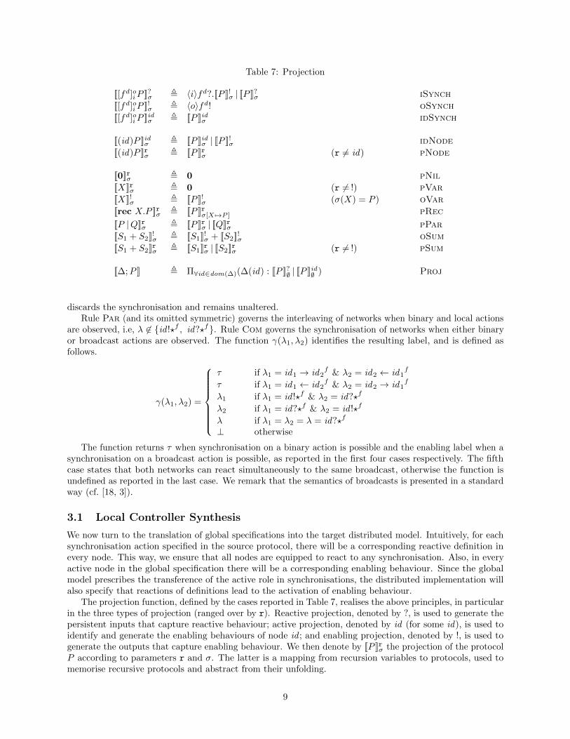
Table 7: Projection

[[[fd]oiP ]]?σ , 〈i〉fd?.[[P ]]!σ | [[P ]]?σ iSynch

[[[fd]oiP ]]!σ , 〈o〉fd! oSynch

[[[fd]oiP ]]idσ , [[P ]]idσ idSynch

[[(id)P ]]idσ , [[P ]]idσ | [[P ]]!σ idNode

[[(id)P ]]rσ , [[P ]]rσ (r 6= id) pNode

[[0]]rσ , 0 pNil

[[X]]rσ , 0 (r 6= !) pVar

[[X]]!σ , [[P ]]!σ (σ(X) = P ) oVar

[[rec X.P ]]rσ , [[P ]]rσ[X 7→P ] pRec

[[P |Q]]rσ , [[P ]]rσ | [[Q]]rσ pPar

[[S1 + S2]]!σ , [[S1]]!σ + [[S2]]!σ oSum

[[S1 + S2]]rσ , [[S1]]rσ | [[S2]]rσ (r 6= !) pSum

[[∆;P ]] , Π∀id∈dom(∆)(∆(id) : [[P ]]?∅ | [[P ]]id∅ ) Proj

discards the synchronisation and remains unaltered.Rule Par (and its omitted symmetric) governs the interleaving of networks when binary and local actions

are observed, i.e, λ 6∈ {id !?f , id??f}. Rule Com governs the synchronisation of networks when either binaryor broadcast actions are observed. The function γ(λ1, λ2) identifies the resulting label, and is defined asfollows.

γ(λ1, λ2) =

τ if λ1 = id1 → id2f & λ2 = id2 ← id1

f

τ if λ1 = id1 ← id2f & λ2 = id2 → id1

f

λ1 if λ1 = id !?f & λ2 = id??f

λ2 if λ1 = id??f & λ2 = id !?f

λ if λ1 = λ2 = λ = id??f

⊥ otherwise

The function returns τ when synchronisation on a binary action is possible and the enabling label when asynchronisation on a broadcast action is possible, as reported in the first four cases respectively. The fifthcase states that both networks can react simultaneously to the same broadcast, otherwise the function isundefined as reported in the last case. We remark that the semantics of broadcasts is presented in a standardway (cf. [18, 3]).

3.1 Local Controller Synthesis

We now turn to the translation of global specifications into the target distributed model. Intuitively, for eachsynchronisation action specified in the source protocol, there will be a corresponding reactive definition inevery node. This way, we ensure that all nodes are equipped to react to any synchronisation. Also, in everyactive node in the global specification there will be a corresponding enabling behaviour. Since the globalmodel prescribes the transference of the active role in synchronisations, the distributed implementation willalso specify that reactions of definitions lead to the activation of enabling behaviour.

The projection function, defined by the cases reported in Table 7, realises the above principles, in particularin the three types of projection (ranged over by r). Reactive projection, denoted by ?, is used to generate thepersistent inputs that capture reactive behaviour; active projection, denoted by id (for some id), is used toidentify and generate the enabling behaviours of node id ; and enabling projection, denoted by !, is used togenerate the outputs that capture enabling behaviour. We then denote by [[P ]]rσ the projection of the protocolP according to parameters r and σ. The latter is a mapping from recursion variables to protocols, used tomemorise recursive protocols and abstract from their unfolding.

9

We briefly explain the cases in Table 7. Case iSynch shows the reactive projection of the synchronisationaction, yielding a persistent input with the respective condition i, label f , and direction d. The continuationof the input is obtained by the enabling projection (!) of the continuation of the synchronisation action (P ).Hence, the reaction leads to the enabling of the continuation which captures the transference of the activerole in synchronisations. The result of the projection also specifies the (simultaneously active | ) reactiveprojection of the continuation protocol, so as to generate the corresponding persistent inputs. Case oSynchshows the enabling projection of the synchronisation action, yielding the output considering the respectivecondition o, label f , and direction d. Notice that the fact that outputs do not specify continuations is alignedwith the idea that a node yields the active role after enabling a synchronisation.

Case idSynch shows the active projection of the synchronisation action, yielding the active projection ofthe continuation. The idea is that active projection inspects the structure of the protocol, and introducesenabling behaviour whenever an active node construct specifying the respective id is found (i.e., (id)P ). Thisis made precise in case idNode, where the projection yields both the enabling projection of the protocol Ptogether with its the active projection, so as to address configurations in which the same node is active indifferent stages of the protocol. Case pNode instead shows that the other types of projection of the activenode construct result in the respective projection of the continuation.

Case pNil says that the terminated protocol is projected (in all types of projection) to inaction (0).Case pVar says that the active/reactive projections of the recursion variable also yield inaction, hence donot require reasoning on the unfolding. Instead, case oVar shows the enabling projection of the recursionvariable, yielding the enabling projection of the variable mapping, which allows to account for the unfolding.This is made precise in case pRec where the mapping is updated with the association of the variable mapsto the recursion body.

We remark that well-formed protocols do not specify active node constructs in the body of a recursion,since they originate from protocols where all active node constructs are top-level, hence the active projectionof any recursive protocol necessarily yields inaction (nevertheless captured in the general case).

Case pPar says that (all types of) projection of the fork protocol yields the (simultaneously active)respective projections of the branches of the fork. Cases oSum and pSum address the summation protocol:on the one hand, the enabling projection yields the choice between the projections of the branches; on theother hand, reactive/active projection yield the simultaneously active projections of the branches. Notice thatchoices may only specify outputs, hence only enabling projection may yield alternative (output) behaviour.Reactive projection yields a collection of persistent inputs (one per synchronisation action) which aresimultaneously active. Active projection generates the enabling behaviour of active nodes, so if such activenodes are found in (continuations of) the branches of the summation, their enabling behaviour is taken assimultaneously active.

The projection of a configuration, denoted [[∆;P ]] and defined in the Proj case, specifies a parallelcomposition of all nodes of the network (i.e., all those comprised in the network state). Each node is obtainedby considering the state yielded by the respective network state mapping, and considering the behaviouris yielded by a combination of the reactive and the active projections of the protocol P . Notice that theactive projection is carried out considering the node identifier, hence the result potentially differs betweendistinct nodes, while the reactive projection is exactly the same for all nodes. Intuitively, consider the reactiveprojection as the static collection of reactive definitions, and the active projection as the runtime (immediatelyavailable) enabling behaviour.

Example 3.1. The reactive projection of the Simple protocol in Sect. 1.1(1) is

[[Simple]]?∅ = 〈c1 ∨ c2〉Locate??.(〈c1〉Locate?! + 〈c2〉RecoverN!

)| 〈tt〉RecoverN?.0

For the purpose of our operational correspondence result, we consider structural congruence of networksand of behaviours defined by the rules shown in Table 8. The rules capture expected principles (namely, thatoperators ‖ , | , and + are associative and commutative, and that | has identity element 0) and an absorbingprinciple for persistent inputs (i.e., 〈i〉fd?.R | 〈i〉fd?.R ≡ 〈i〉fd?.R), which allows to reason about persistentinputs as if they are unique, necessary when considering the reacting projection of a recursive protocol and

its unfolding. We may now state our operational correspondence result, where we denote by N1λ−→≡ N2 that

there exists N ′ such that N1λ−→ N ′ and N ′ ≡ N2, and where we use λ to range over id !?f and τ labels.

10

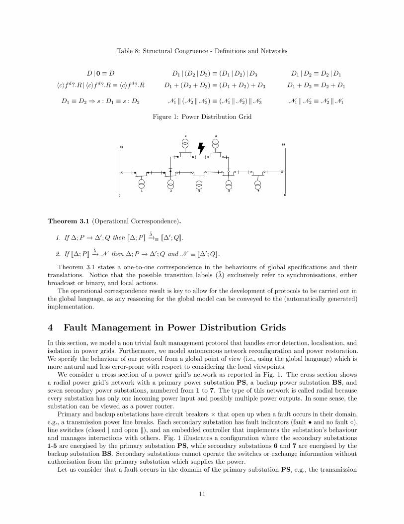
Table 8: Structural Congruence - Definitions and Networks

D |0 ≡ D D1 | (D2 |D3) ≡ (D1 |D2) |D3 D1 |D2 ≡ D2 |D1

〈c〉fd?.R | 〈c〉fd?.R ≡ 〈c〉fd?.R D1 + (D2 +D3) ≡ (D1 +D2) +D3 D1 +D2 ≡ D2 +D1

D1 ≡ D2 ⇒ s : D1 ≡ s : D2 N1 ‖ (N2 ‖N3) ≡ (N1 ‖N2) ‖N3 N1 ‖N2 ≡ N2 ‖N1

Figure 1: Power Distribution Grid

Theorem 3.1 (Operational Correspondence).

1. If ∆;P −→ ∆′;Q then [[∆;P ]]λ−→≡ [[∆′;Q]].

2. If [[∆;P ]]λ−→ N then ∆;P −→ ∆′;Q and N ≡ [[∆′;Q]].

Theorem 3.1 states a one-to-one correspondence in the behaviours of global specifications and theirtranslations. Notice that the possible transition labels (λ) exclusively refer to synchronisations, eitherbroadcast or binary, and local actions.

The operational correspondence result is key to allow for the development of protocols to be carried out inthe global language, as any reasoning for the global model can be conveyed to the (automatically generated)implementation.

4 Fault Management in Power Distribution Grids

In this section, we model a non trivial fault management protocol that handles error detection, localisation, andisolation in power grids. Furthermore, we model autonomous network reconfiguration and power restoration.We specify the behaviour of our protocol from a global point of view (i.e., using the global language) which ismore natural and less error-prone with respect to considering the local viewpoints.

We consider a cross section of a power grid’s network as reported in Fig. 1. The cross section showsa radial power grid’s network with a primary power substation PS, a backup power substation BS, andseven secondary power substations, numbered from 1 to 7. The type of this network is called radial becauseevery substation has only one incoming power input and possibly multiple power outputs. In some sense, thesubstation can be viewed as a power router.

Primary and backup substations have circuit breakers × that open up when a fault occurs in their domain,e.g., a transmission power line breaks. Each secondary substation has fault indicators (fault • and no fault ◦),line switches (closed | and open ‖), and an embedded controller that implements the substation’s behaviourand manages interactions with others. Fig. 1 illustrates a configuration where the secondary substations1-5 are energised by the primary substation PS, while secondary substations 6 and 7 are energised by thebackup substation BS. Secondary substations cannot operate the switches or exchange information withoutauthorisation from the primary substation which supplies the power.

Let us consider that a fault occurs in the domain of the primary substation PS, e.g., the transmission

11

power line between substations 3 and 4 breaks. The primary substation can sense the existence of a faultbecause its circuit breaker × opens up, but it cannot determine the location of the fault. Hence, the substationPS initiates the fault recovery protocol by synchronising with its directly connected secondary substations anddelegates them to activate the local fault recovery protocol. The delegation between secondary substationspropagates in the direction given by their fault indicators.

A secondary substation first validates the error signal by measuring its voltage level. If the voltage iszero, the secondary substation activates the fault recovery protocol, otherwise the signal is discarded. Once asecondary substation activates the fault recovery protocol, it inspects its own fault indicators and determineswhether the fault is on its input or output power lines. If the fault is on its output, it delegates the substationsconnected to its output power lines to collaborate to locate the fault. If the fault is on its input power line,the substation (in our case, substation 4) takes control and initiates both isolation and power restoration.The former consists of isolating the faulty line and restoring the power to the network’s segment locatedbefore the fault, while the latter consists of restoring the power to the network’s segment located after thefault.

For isolation, substation 4 opens its switches to the faulty line segment and collaborates with 3 to openits affected line switches as well. Notice that now the domain of the primary substation PS is segmentedinto two islands: {PS,1,2,3,5} and {4}. The control is transferred back to the primary substation in astep by step fashion and the power is restored to the first island. For power restoration, substation 4 asksfor power supply from one of its neighbours that is capable of supplying an additional substation (in ourcase, substation 6). Once substation 6 supplies power to 4, the latter changes its power source to 6 and nowsubstation 4 belongs to the domain of the backup substation BS.

We now show how to provide a simple and intuitive global specification for our scenario using the linguisticprimitives of the global language. In what follows, we use the following terminology: the state of a sourcelink t can be 0 (to indicate a faulty link) or 1 otherwise. We will use z in place of the source id when asubstation is not connected to a power supply. The initial state of each substation follows from Fig. 1. Forinstance, substations 3, 4, and 6 have the following initial states 3[2, 1, {2, 4}, 1, 1, 1], 4[3, 0, {3, 6}, 1, 0, 0],and 6[7, 1, {4, 5, 7}, 2, 0, 0], respectively. The recovery protocol is reported below.

Recovery , rec X.([Locate?]o1i1X + [End•]o2i2 Islanding)

Islanding , IsolationStart |Restoration

The protocol states that either Locate is broadcasted to the children of the enabling substation, afterwhich the protocol starts over, or End is carried out and the node retains control. In case End is carried out,the enabling substation proceeds by activating the Islanding protocol. The latter specifies a fork betweenIsolationStart and the Restoration protocols.

A substation enabled on Recovery can broadcast Locate only when it has at least one faulty output,i.e., o1 = (e > 0). Furthermore, receiving substations can synchronise on Locate only if they have fault ontheir output or their input, i.e., i1 = (e > 0) ∨ (t = 0). On the other hand, End can be carried out when theenabling substation has a fault on its input, i.e., o2 = (t = 0) and i2 = tt. Both actions have no side-effectson states.

The Isolation and the Restoration protocols are reported below:

IsolationStart , [RecoverN]o3i3 0 + [RecoverDoneN]o3i4 Isolation

Isolation , rec X.([IsolateN]o5i3 0 + [IsolateDoneN]o5i4X + [Stop•]o6i2 0))

Restoration , [PowerI]o7i7 0

The IsolationStart protocol states that a synchronisation between the enabling substation and itsparent on the Recover or RecoverDone actions may happen only if the enabling substation has a fault on itsinput, i.e., o3 = (t = 0). The parent reacts on Recover if the number of faults on its output is greater thanone, i.e., i3 = (e > 1). In this case the parent does not proceed, since there are still more faulty links tobe handled. Instead, the RecoverDone synchronisation captures the case for the handling of the last faultylink, i.e., i4 = (e = 1), in which case the parent takes control and proceeds to Isolation. In both cases, theenabling station disconnects itself from the faulty line (setting parent to z) and the parent decrements itsoutput faults (e), its active outputs (a), and also its capacity (k). Furthermore, both enabling and parentnode remove each other from the list of neighbours, thus isolating the faulty link.

12

When the parent is enabled on Isolation then three synchronisation branches on the Isolate, theIsolateDone and the Stop actions can be carried out. An enabling substation can synchronise with its parenton an Isolate or IsolateDone actions if it is not the primary station, i.e., o5 = (i 6= ∞). As a side-effect onthe state of the parent, the number of faults is decremented (e). Notice that the interpretation of the twobranches on Isolate and IsolateDone is similar to the one on Recover and RecoverDone. Only the primarystation (o6 = (i =∞)) can execute the Stop action, ending the Isolation protocol. As mentioned before,local actions have no side-effects.

Finally, the Restoration protocol states that a disconnected substation, i.e., o7 = (i = z), can synchronisewith one of its neighbours (I) on the Power action as a request for a power supply. Only a neighbour thathas enough power and is fully functional (i7 = (k > a ∧ e = 0)) can engage in the synchronisation. Bydoing so, the neighbour increments its active outputs (a) and the enabling substation marks its neighbouras its power source. The protocol then terminates after the network reconfiguration. Note that althoughthe IsolationStart and the Restoration protocols are specified in parallel, a specific order is actuallyinduced by the synchronisation conditions. Thanks to the output condition o7 = (i = z) of the Power action,we are sure that the power supply can be reestablished only after the faulty link is disconnected, which is aside-effect of either Recover or RecoverDone actions. Thus, the synchronisation on Power can only happenafter the synchronisation on either Recover or RecoverDone.

The static protocol Recovery abstracts from the concrete network configuration. To represent a concretegrid network, active substations must be added at “top-level” to the Recovery protocol, together with thenetwork state, i.e., ∆; (PS)Recovery where ∆ is a mapping from a substation identifiers to states. Noticethat the primary station, PS, is initially active because, according to our scenario, it is the only station thathas rights to initiate protocols.

We remark that the protocol is designed so as to handle configurations with multiple faults, where severalnodes may be active simultaneously on, e.g., Locate albeit belonging to different parts (subtrees) of thenetwork.

5 Concluding Remarks

We propose a model of interaction for power distribution grids. More precisely, we show how to specifyoperation control protocols governing the behaviour of a power gird as a whole from a global perspective.We formalise how global model specifications can be used to automatically synthesise individual controllersof the grid substations, yielding an operationally correct distributed implementation. We also show how touse our global language to model a non-trivial fault management scenario from the realm of power girds.Notice that the design principles of our model target power distribution grids specifically, namely consideringthat interaction is confined to closely follow the network topology. However, the principles showcased by ourdevelopment can be used when considering other topologies. Conceivably, our principles can also be conveyedto other settings where operation protocols involve yielding control as a consequence of synchronisations.We conclude this paper by relating to existing literature, focusing on formal models in particular, and bymentioning some directions for future work.

Global protocol specifications can be found in the session type literature, spawning from the work of Hondaet al. [19]. Such specifications are typically used to verify programs or guide their development. More recently,we find proposals that enrich the global protocol specifications so as to allow programming to be carried outdirectly in the global language (e.g., choreographies [11]). We insert our development in this context, sincewe also provide a global specification language where operation control protocols can be programmed. Thedistinguishing features of our approach naturally stem from the targeted setting. In particular, we considerthat protocol specifications are role-agnostic and that the interacting parties are established operationally inthe following sense: emitting/enabling parties are determined from active nodes and receiving/reacting partiesare determined by the network topology, and the active role is transferred in synchronisations. Previoussession-type based approaches typically consider protocols include role annotations, which are impersonatedby parties at runtime when agreeing to collaborate on a protocol. Some works also consider role-agnosticprotocol specifications [10], that roles have a more flexible interpretation, for instance that the associationbetween party and role is dynamic [8] and that several parties may simultaneously impersonate a singlerole [17]. None of such works, as far as we know, considers that the receiver is determined by the combination

13

of who is the sender and the network topology, and that control is yielded in communication.For future work, it is definitely of interest to develop verification techniques for system level safety

properties, and it seems natural to specify and check such properties considering the global model. To reasonon protocol correctness and certify operation on all possible configurations, such verification techniques shouldfocus on the static specification and abstract from the concrete network configuration, relying in some formof abstract interpretation [14, 15]. Thanks to the operational correspondence result that relates the globaland distributed models, we can ensure that any property that holds for the global specification also holds forthe distributed one. The reactive style of the distributed model suggests an implementation based on theactor model [4] (in, e.g., Erlang [7]). Conceivably, such reactive descriptions can be useful in other realms, inparticular when addressing interaction models based on immediate reactions to external stimulus.

A Operational Correspondence

In this section, we sketch the proof of operational correspondence, separating the proof of soundness(Lemma A.13) and completeness (Lemma A.29) in two subsections (Section A.1 and Section A.2, respectively).

A.1 Operational Correspondence - Soundness

We introduce auxiliary lemmas to structure the proof. The following lemma ensures that structurallyequivalent networks have equivalent behaviours.

Lemma A.1 (Definition and Network LTS Closure Under Structural Congruence).

1. If D1α−→ D′1 and D1 ≡ D2 then D2

α−→≡ D′1.

2. If N1λ−→ N ′

1 and N1 ≡ N2 then N2λ−→≡ N ′

1 .

Proof. The proof follows by induction on the length of the derivation D1 ≡ D2 and N1 ≡ N2 in expectedlines, where 2 relies on 1 .

The following results are used in the proof that structural congruence is preserved by projection, inparticular regarding recursion unfolding. We start by addressing properties of the !-projection, namely,Lemma A.2 shows that it is preserved under any environment and process substitution since only the initialactions are relevant.

Lemma A.2 (Preservation of !-Projection). Let P be a protocol where recursion is guarded. We have that

1. [[P ]]!σ ≡ [[P ]]!σ′ for any σ, σ′.

2. [[P [Q/X]]]!σ ≡ [[P ]]!σ.

Proof. By induction on the structure of P following expected lines. Notice that !-projection addresses onlyimmediate synchronisation actions, hence neither the mapping σ nor the substitution affect the projectiongiven that recursion is guarded in P .

Lemma A.2 is used directly in the proof of recursion unfolding for the !-projection and also to proveproperties of the ?-projection. Lemma A.3 is also auxiliary to the case of ?-projection, showing thecorrespondence between environment and process substitution used in !-projection.

Lemma A.3 (Soundness of Mapping for !-Projection). Let Q be a protocol where recursion in guarded. Wehave that [[P ]]!σ[X 7→Q] ≡ [[P [Q/X]]]!σ.

Proof. By induction on the structure of P following expected lines. Notice that when P is X then we obtain[[Q]]!σ[X 7→Q] and [[Q]]!σ which may be equated considering Lemma A.2(1 ).

We now address properties that directly regard the ?-projection, starting by Lemma A.4 that shows thatprocesses in the environment are interchangeable as long as their !-projection is equivalent.

14

Lemma A.4 (Preservation of ?-Projection). Let Q1 and Q2 be protocols where recursion is guarded suchthat [[Q1]]!σ ≡ [[Q2]]!σ. We have that [[P ]]?σ[X 7→Q1] ≡ [[P ]]?σ[X 7→Q2].

Proof. By induction on the structure of P following expected lines. Notice that when P is X then we obtain[[Q1]]!σ[X 7→Q1] and [[Q2]]!σ[X 7→Q2] which may be equated considering Lemma A.2(1 ) and the hypothesis.

The following result (Lemma A.5) is key to the proof of the unfolding, as it shows that two copies of a?-projection are equivalente to one.

Lemma A.5 (Replicability of ?-Projection). We have that [[P ]]?σ | [[P ]]?σ ≡ [[P ]]?σ.

Proof. By induction on the structure of P . The proof follows by induction hypothesis in expected lines forall cases except for the synchronisation action which also relies on axiom 〈c〉fd?.R | 〈c〉fd?.R ≡ 〈c〉fd?.R.

The main auxiliary properties for the case of recursion unfolding regarding ?-projection are given by thenext result. Lemma A.6(1 ) equates the substitution with the environment, considering the involved processis in context. Lemma A.6(2 ) equates the substitution with the environment, considering a context with some(input) residua.

Lemma A.6 (Soundness of Mapping for ?-Projection). Let Q be a protocol where recursion is guarded.

1. We have that [[P ]]?σ[X 7→Q] | [[Q]]?σ ≡ [[P [Q/X]]]?σ | [[Q]]?σ.

2. We have that [[P [Q/X]]]?σ ≡ [[P ]]?σ[X 7→Q] |Πi∈I〈ci〉fdii ?.Ri.

Proof. By induction on the structure of P . We sketch the proof of 1., the proof of 2. follows similar lines.

Case P is 0 We have that 0 | [[Q]]?σ ≡ 0 | [[Q]]?σ.

Case P is X Since [[X]]?σ[X 7→Q] by definition is 0, we have that 0 | [[Q]]?σ ≡ [[Q]]?σ | [[Q]]?σ and the proof followsby considering Lemma A.5.

Case P is (id)P ′ or P1 |P2 or S1 + S2 The proof follows from the induction hypothesis in expected lines.

Case P is [fd]oiP′ Since [[[fd]oiP

′]]?σ[X 7→Q] by definition is 〈i〉fd?.[[P ′]]!σ[X 7→Q] | [[P′]]?σ[X 7→Q] we have that (i)

[[[fd]oiP′]]?σ[X 7→Q] | [[Q]]?σ ≡ 〈i〉fd?.[[P ′]]!σ[X 7→Q] | [[P

′]]?σ[X 7→Q] | [[Q]]?σ. Considering Lemma A.3 we have

that (ii) 〈i〉fd?.[[P ′]]!σ[X 7→Q] ≡ 〈i〉fd?.[[P ′[Q/X]]]!σ. By induction hypothesis we conclude that (iii)

[[P ′]]?σ[X 7→Q] | [[Q]]?σ ≡ [[P ′[Q/X]]]?σ | [[Q]]?σ. Considering both (ii) and (iii) we conclude that (iv)

〈i〉fd?.[[P ′]]!σ[X 7→Q] | [[P′]]?σ[X 7→Q] | [[Q]]?σ ≡ 〈i〉fd?.[[P ′[Q/X]]]!σ | [[P ′[Q/X]]]?σ | [[Q]]?σ

By definition we have that [[[fd]oiP′[Q/X]]]?σ | [[Q]]?σ ≡ 〈i〉fd?.[[P ′[Q/X]]]!σ | [[P ′[Q/X]]]?σ | [[Q]]?σ which

considering (i) and (iv) completes the proof.

Case P is rec X.P ′ By definition we have that [[rec X.P ′]]?σ[X′ 7→Q] | [[Q]]?σ ≡ [[P ′]]?σ[X′ 7→Q][X 7→P ′] | [[Q]]?σ. By

induction hypothesis we have that [[P ′]]?σ[X′ 7→Q][X 7→P ′] | [[Q]]?σ ≡ [[P ′[Q/X ′]]]?σ[X 7→P ′] | [[Q]]?σ. Considering

Lemma A.2(2 ) since recursion is guarded in P ′ we have that [[P ′[Q/X ′]]]!σ ≡ [[P ′]]!σ, from which, consider-ing Lemma A.4, we conclude [[P ′[Q/X ′]]]?σ[X 7→P ′] | [[Q]]?σ ≡ [[P ′[Q/X ′]]]?σ[X 7→(P ′[Q/X′])] | [[Q]]?σ. The latter

concludes the proof since by definition [[rec X.P ′[Q/X]]]?σ | [[Q]]?σ ≡ [[P ′[Q/X ′]]]?σ[X 7→(P ′[Q/X′])] | [[Q]]?σ.

The following result is used in the proof of the id -projection.

Lemma A.7 (Static Protocol id -Projection). Let P be an (id)-absent protocol. We have that [[P ]]idσ ≡ 0.

Proof. By induction on the structure of P following expected lines.

15

We may now prove that projection is preserved under recursion unfolding. This lemma will be used in theproof of Lemma A.9, where we want to show that the projection function is invariant to structural congruentprotocols.

Lemma A.8 (Preservation of Projection under Unfolding). Let P be an (id)-absent protocol where recursionis guarded. We have that [[rec X.P ]]r∅ ≡ [[P [rec X.P/X]]]r∅ for any r.

Proof. We prove the three cases separately.

Case r = ! By definition we have [[rec X.P ]]!∅ , [[P ]]![X 7→P ]. Since recursion is guarded in P , from Lemma A.2(2 )

we conclude [[P ]]![X 7→P ] ≡ [[P [rec X.P/X]]![X 7→P ], and from Lemma A.2(1 ) we have [[P [rec X.P/X]]![X 7→P ] ≡[[P [rec X.P/X]]!∅.

Case r = id Since P is an (id)-absent protocol we have that P [rec X.P/X] is an (id)-absent protocol,hence the result follows immediately from Lemma A.7 from which we conclude [[rec X.P ]]id∅ ≡ 0 and

[[P [rec X.P/X]]]id∅ ≡ 0.

Case r = ? From Lemma A.6(1 ) we have that

[[P ]]?[X 7→rec X.P ] | [[rec X.P ]]?∅ ≡ [[P [rec X.P/X]]]?∅ | [[rec X.P ]]?∅

By definition we have that [[rec X.P ]]!∅ ≡ [[P ]]![X 7→P ] and since recursion is guarded in P from

Lemma A.2(1 ) we have that [[P ]]![X 7→P ] ≡ [[P ]]!∅ hence [[rec X.P ]]!∅ ≡ [[P ]]!∅. From this fact, consid-ering Lemma A.4 we conclude

[[P ]]?[X 7→P ] | [[rec X.P ]]?∅ ≡ [[P [rec X.P/X]]]?∅ | [[rec X.P ]]?∅

By definition we have that [[rec X.P ]]?∅ ≡ [[P ]]?[X 7→P ], hence

[[rec X.P ]]?∅ | [[rec X.P ]]?∅ ≡ [[P [rec X.P/X]]]?∅ | [[rec X.P ]]?∅

From Lemma A.5 we have that [[rec X.P ]]?∅ | [[rec X.P ]]?∅ ≡ [[rec X.P ]]?∅, hence (i)

[[rec X.P ]]?∅ ≡ [[P [rec X.P/X]]]?∅ | [[rec X.P ]]?∅

From Lemma A.6(2 ) we have that

[[P [rec X.P/X]]]?σ ≡ [[P ]]?σ[X 7→rec X.P ] |Πl∈L〈cl〉fdll ?.Rl

As before, from [[rec X.P ]]!∅ ≡ [[P ]]!∅ and considering Lemma A.4 we conclude

[[P [rec X.P/X]]]?σ ≡ [[P ]]?σ[X 7→P ] |Πl∈L〈cl〉fdll ?.Rl

and, again as before, since by definition [[rec X.P ]]?∅ ≡ [[P ]]?[X 7→P ] we conclude (ii)

[[P [rec X.P/X]]]?σ ≡ [[rec X.P ]]?∅ |Πl∈L〈cl〉fdll ?.Rl

which together with (i)[[rec X.P ]]?∅ ≡ [[P [rec X.P/X]]]?∅ | [[rec X.P ]]?∅

allows us to conclude

[[rec X.P ]]?∅ ≡ [[rec X.P ]]?∅ |Πl∈L〈cl〉fdll ?.Rl | [[rec X.P ]]?∅

From this fact and considering Lemma A.5 we conclude

[[rec X.P ]]?∅ ≡ [[rec X.P ]]?∅ |Πl∈L〈cl〉fdll ?.Rl

which together with (ii)

[[P [rec X.P/X]]]?σ ≡ [[rec X.P ]]?∅ |Πl∈L〈cl〉fdll ?.Rl

completes the proof.

16

Lemma A.9 states that structurally congruent protocols have structurally congruent projections, namelyequivalent reactive projection “?”, active projection “id” and output projection “!”. This lemma will be usedin the proof of the soundness lemma, Lemma A.13.

Lemma A.9 (Preservation of Projection Under Structural Congruence). If P ≡ Q then [[P ]]r∅ ≡ [[Q]]r∅ forany r.

Proof. The proof proceeds by induction on the length of the derivation P ≡ Q.

Case P is Q |0 We need to prove that [[Q |0]]r∅ ≡ [[Q]]r∅ for any r. We have three cases depending on r.

Case r =?: By definition of the projection function, we have that

[[Q |0]]?∅ = [[Q]]?∅ | [[0]]?∅

By the definition again, we know that [[0]]?∅ = 0 and now we have that [[Q |0]]?∅ ≡ [[Q]]?∅ |0 ≡ [[Q]]?∅as required.

Case r =!: By definition of the projection function, we have that

[[Q |0]]!∅ = [[Q]]!∅ | [[0]]!∅

By the definition again, we know that [[0]]!∅ = 0 and now we have that [[Q |0]]!∅ ≡ [[Q]]!∅ |0 ≡ [[Q]]!∅as required.

Case r = id : By definition of the projection function, we have that

[[Q |0]]id∅ = [[Q]]id∅ | [[0]]id∅

By the definition again, we know that [[0]]id∅ = 0 and now we have that [[Q |0]]id∅ ≡ [[Q]]id∅ |0 ≡ [[Q]]id∅as required.

Case P is Q1 | (Q2 |Q3) We need to prove that [[Q1 | (Q2 |Q3)]]r∅ ≡ [[(Q1 |Q2) |Q3]]r∅ for any r. We have threecases depending on r.

Case r =?: By definition of the projection function, we have that

[[Q1 | (Q2 |Q3)]]?∅ = [[Q1]]?∅ | [[Q2 |Q3]]?∅ = [[Q1]]?∅ | [[Q2]]?∅ | [[Q3]]?∅

and

[[(Q1 |Q2) |Q3]]?∅ = [[Q1 |Q2]]?∅ | [[Q3]]?∅ = [[Q1]]?∅ | [[Q2]]?∅ | [[Q3]]?∅ as required.

Case r ∈ {!, id}: Similar to the case of “?”.

Cases where P is Q1 + (Q2 +Q3), Q1 +Q2, Q1 |Q2, (id)0: follow directly by the definition.

Case P is (id)(Q1 |Q2) We need to prove that [[(id)(Q1 |Q2)]]r∅ ≡ [[(id)Q1]]r∅ | [[(id)Q2]]r∅ for any r. We havethree cases depending on r.

Case r =?: By definition of the projection function, we have that

[[(id)(Q1 |Q2)]]?∅ = [[Q1 |Q2]]?∅ = [[Q1]]?∅ | [[Q2]]?∅

[[(id)Q1]]?∅ | [[(id)Q2]]?∅ = [[Q1]]?∅ | [[Q2]]?∅ as required.

Case r =!: Similar to the case of “?”.

17

Case r = id : We have two cases: r 6= id or r = id . The former case is similar to {?, !} while the lattercase can be proved as follows;

[[(id)(Q1 |Q2)]]id∅ = [[Q1 |Q2]]id∅ | [[Q1 |Q2]]!∅ = [[Q1]]id∅ | [[Q2]]id∅ | [[Q1]]!∅ | [[Q2]]!∅

[[(id)Q1]]id∅ | [[(id)Q2]]id∅ = [[Q1]]id∅ | [[Q1]]!∅ | [[Q2]]id∅ | [[Q2]]!∅

And we have that [[Q1]]id∅ | [[Q2]]id∅ | [[Q1]]!∅ | [[Q2]]!∅ ≡ [[Q1]]id∅ | [[Q1]]!∅ | [[Q2]]id∅ | [[Q2]]!∅ as required.

Case P is (id1)(id2)Q We need to prove that [[(id1)(id2)Q]]r∅ ≡ [[(id2)(id1)Q]]r∅ for any r. We have threecases depending on r.

Cases r ∈ {?, !}: By defintion [[(id1)(id2)Q]]?∅ ≡ [[(id2)(id1)Q]]?∅ = [[(id1)(id2)Q]]!∅ ≡ [[(id2)(id1)Q]]!∅ =

[[Q]]?∅ = [[Q]]!∅Case r = id : We have three cases:

1) id 6= id1 ∧ id 6= id2: By defintion we have that [[(id1)(id2)Q]]id∅ ≡ [[(id2)(id1)Q]]id∅ = [[Q]]id∅ .

2) id = id1: By definition we have that:

[[(id1)(id2)Q]]id1

∅ = [[(id2)Q]]id1

∅ | [[(id2)Q]]!∅ = [[Q]]id1

∅ | [[Q]]!∅

[[(id2)(id1)Q]]id1

∅ = [[(id1)Q]]id1

∅ = [[Q]]id1

∅ | [[Q]]!∅ as required.

3) id = id2: Similar to case (2).

Case P is rec X.Q We need to prove that [[rec X.Q]]r∅ ≡ [[Q[rec X.Q/X]]]r∅ for any r. Directly by LemmaA.8.

Lemma A.10 states basically that the projection function is invariant to reduction in the case of outputand reactive projections. We will use this result mainly in the proof of the main theorem.

Lemma A.10 (Preservation of !/?-Projections Under Reduction). If ∆;P −→ ∆′;Q then [[P ]]r ≡ [[Q]]r wherer ∈ {!, ?}.

Proof. By induction on the length of the derivation ∆;P −→ ∆′;Q.

Case 1: Rule Bin is applied: We have that ∆; (id)([fd]oiP + S) −→∆′; [fd]oi ((id

′)P ) + S and we need to prove that [[(id)([fd]oiP + S)]]r∅ ≡ [[[fd]oi ((id ′)P ) + S]]r∅. We havedifferent cases:

Case r =?: By definition of the projection function, we have that

[[(id)([fd]oiP + S)]]?∅ = 〈i〉fd?.[[P ]]!∅ | [[P ]]?∅ | [[S]]?∅

[[[fd]oi ((id′)P ) + S]]?∅ = 〈i〉fd?.[[(id′)P ]]!∅ | [[(id

′)P ]]?∅ | [[S]]?∅

By definition again, we know that [[(id′)P ]]!∅ = [[P ]]!∅ and [[(id′)P ]]?∅ = [[P ]]?∅ and we have that

[[(id)([fd]oiP + S)]]?∅ ≡ [[[fd]oi ((id′)P ) + S]]?∅ as required.

Case r =!: By definition of the projection function, we have that

[[(id)([fd]oiP + S)]]!∅ = 〈o〉fd! + [[S]]!∅

[[[fd]oi ((id′)P ) + S]]!∅ = [[[fd]oi ((id

′)P )]]!∅ + [[S]]!∅

By definition again, we know that [[[fd]oi ((id′)P )]]!∅ = 〈o〉fd! and we have that [[(id)([fd]oiP +S)]]!∅ ≡

[[[fd]oi ((id′)P ) + S]]!∅ as required.

Case 2 Rules Brd and Loc can be proved in a similar manner.

18

Case 3 Rule Synch: We need to prove that if ∆; [fd]oiP −→ ∆′; [fd]oiP′ then [[[fd]oiP ]]r∅ ≡ [[[fd]oiP

′]]r∅. Wehave different cases:

Case r =?: By definition of the projection function, we have that

[[[fd]oiP ]]?∅ = 〈i〉fd?.[[P ]]!∅ | [[P ]]?∅

[[[fd]oiP′)]]?∅ = 〈i〉fd?.[[P ′]]!∅ | [[P

′]]?∅

By the induction hypothesis, we have that [[P ′]]!∅ = [[P ]]!∅ and [[P ′]]?∅ = [[P ]]?∅ and we have that

[[[fd]oiP ]]?∅ ≡ [[[fd]oiP′]]?∅ as required.

Case r =!: By definition of the projection function, we have that

[[[fd]oiP ]]!∅ = [[[fd]oiP′]]!∅ = 〈o〉fd!

and we have that [[[fd]oiP ]]!∅ ≡ [[[fd]oiP′]]!∅ as required.

Case 4 Rule Id: We need to prove that if ∆; (id)P −→ ∆′; (id)P ′ then [[(id)P ]]r∅ ≡ [[(id)P ′]]r∅. We havedifferent cases:

Case r =?: By definition of the projection function, we have that

[[(id)P ]]?∅ = [[P ]]?∅ and [[(id)P ′)]]?∅ = [[P ′]]?∅

By the induction hypothesis, we have that [[P ′]]?∅ = [[P ]]?∅ and we have that [[(id)P ]]?∅ ≡ [[(id)P ′]]?∅ asrequired.

Case r =!: By definition of the projection function, we have that

[[(id)P ]]!∅ = [[P ]]!∅ and [[(id)P ′)]]!∅ = [[P ′]]!∅

By the induction hypothesis, we have that [[P ′]]!∅ = [[P ]]!∅ and we have that [[(id)P ]]!∅ ≡ [[(id)P ′]]!∅ asrequired.

Case 5 Rule Sum: We need to prove that if ∆;P1 + P2 −→ ∆′;P ′1 + P2 then [[P1 + P2]]r∅ ≡ [[P ′1 + P2]]r∅. Wehave different cases:

Case r =?: By definition of the projection function, we have that

[[P1 + P2]]?∅ = [[P1]]?∅ | [[P2]]?∅

[[P ′1 + P2]]?∅ = [[P ′1]]?∅ | [[P2]]?∅

By the induction hypothesis, we have that [[P ′1]]?∅ = [[P1]]?∅ and we have that [[P1 + P2]]?∅ ≡ [[P ′1 + P2]]?∅as required.

Case r =!: By definition of the projection function, we have that

[[P1 + P2]]!∅ = [[P1]]!∅ + [[P2]]!∅

[[P ′1 + P2]]!∅ = [[P ′1]]!∅ + [[P2]]!∅

By the induction hypothesis, we have that [[P ′1]]!∅ = [[P1]]!∅ and we have that [[P1 + P2]]!∅ ≡ [[P ′1 + P2]]!∅as required.

Case 6 Rule Par: We need to prove that if ∆;P1 |P2 −→ ∆′;P ′1 |P2 then [[P1 |P2]]r∅ ≡ [[P ′1 |P2]]r∅. This casecan be proved in a similar manner to the previous case but by using rule Par instead of rule Sum.

Case 7 Rule Struct: We need to prove that if ∆;P −→ ∆′;Q then [[P ]]r∅ ≡ [[Q]]r∅.

From rule Struct, we have that ∆;P −→ ∆′;Q if ∆;P ′ −→ ∆′;Q′ where P ′ ≡ P and Q′ ≡ Q. By theinduction hypothesis we have that [[P ′]]r∅ ≡ [[Q′]]r∅. But P ′ ≡ P and Q′ ≡ Q, so we apply Lemma A.9and conclude the proof.

19

The following Lemma ensures that the parallel composition is merely interleaving and does not influencethe behaviour of any of its sub-definitions, namely if a definition is able to take a step when isolated then thisstep will be possible also when put in parallel with any other definition.

Lemma A.11 (Closure of LTS Under Definition Context). If s : D1λ−→ s′ : D2 then s : D1 |D3

λ−→ s′ : D2 |D3

for any D3.

Proof. By induction on the length of the derivation s : D1 |D3λ−→ s′ : D2 |D3.

Lemma A.12 ensures that structurally equivalent protocols have structurally equivalent projections underany possible network configuration ∆.

Lemma A.12 (Preservation of Structural Congruence Under Network Projection). If P ≡ Q then [[∆;P ]] ≡[[∆;Q]] for any ∆.

Proof. The proof proceeds by relying on the definition of the projection function and Lemma A.9. Bydefinition we have that:

[[∆;P ]] , Π∀id∈dom(∆)(∆(id) : [[P ]]?∅ | [[P ]]id∅ )

[[∆;Q]] , Π∀id∈dom(∆)(∆(id) : [[Q]]?∅ | [[Q]]id∅ )

Since P ≡ Q, we have that, by Lemma A.9 and regardless of ∆, [[P ]]?∅ ≡ [[Q]]?∅ and [[P ]]id∅ ≡ [[Q]]id∅ . Thus[[∆;P ]] ≡ [[∆;Q]] as required.

The soundness of the operational correspondence (i.e., the first statement of Theorem 1) is proved in thefollowing lemma.

Lemma A.13 (Soundness). If ∆;P −→ ∆′;Q then [[∆;P ]]λ−→≡ [[∆′;Q]].

Proof. The proof proceeds by induction on the length of the derivation ∆;P −→ ∆;Q.

Case 1 Rule Bin is applied: We have that ∆; (id)([fd]oiP + S) −→∆′; [fd]oi ((id

′)P ) + S and we need to prove that [[∆; (id)([fd]oiP + S)]]λ−→≡ [[∆′; [fd]oi ((id

′)P ) + S]].

Since a binary interaction happened in the global model, we know that there must be a senderid with ∆(id) = s1 and a receiver id ′ with ∆(id ′) = s2 such that for some d ∈ {N,I} we havethat d(∆, id) = id′, s1 |= o and s2 |= i. As a result of synchronisation on f , we have also thats′1 = fd!(s1, id

′) and s′2 = fd?(s2, id). This can be concluded from the definition of upd(id , id ′, fd,∆)and thus ∆′ = ∆[id 7→ fd!(s1, id

′), id ′ 7→ fd?(s2, id)].

From the definition of the main projection rule in Table 7, we have that:

[[∆;Q]] = N ‖ s1 : [[Q]]?∅ | [[Q]]id∅ ‖ s2 : [[Q]]?∅ | [[Q]]id∅

Where Q = (id)([fd]oiP + S) and N is the rest of the nodes in the network. We do not expand Nbecause it does not contribute to the transition. By Table 7, we have that

s1 : [[Q]]?∅ | [[Q]]id∅ , s1 : 〈i〉fd?.[[P ]]!∅ | [[P ]]?∅ | [[S]]?∅ | | [[P ]]id∅ | [[S]]id∅ | (〈o〉fd! + [[S]]!∅)

s2 : [[Q]]?∅ | [[Q]]id∅ , s2 : 〈i〉fd?.[[P ]]!∅ | [[P ]]?∅ | [[S]]?∅ | [[P ]]id′

∅ | [[S]]id′

∅

The overall network evolves by rule Com where s1 : D1 applies either rule oBinU or rule oBinR ands2 : D2 applies rule iBin, we have that:

N ‖ s1 : [[Q]]?∅ | [[Q]]id∅ ‖ s2 : [[Q]]?∅ | [[Q]]id′

∅τ−→ N ‖ s1 : D′1 ‖ s2 : D′2

20

D′1 = 〈i〉fd?.[[P ]]!∅ | [[P ]]?∅ | [[S]]?∅ | | [[P ]]id∅ | [[S]]id∅

D′2 = 〈i〉fd?.[[P ]]!∅ | [[P ]]!∅ | [[P ]]?∅ | [[S]]?∅ | [[P ]]id′

∅ | [[S]]id′

∅

Now, we need to show that [[∆′; [fd]oi ((id′)P ) + S]] ≡ N ‖ s1 : D′1 ‖ s2 : D′2. By Table 7, we have that

[[∆′;

Q′︷ ︸︸ ︷[fd]oi ((id

′)P ) + S]] = N ‖ s′1 : [[Q′]]?∅ | [[Q′]]id∅ ‖ s

′2 : [[Q′]]?∅ | [[Q

′]]id∅

By applying the projection function, we have that D′1 ≡ [[Q′]]?∅ | [[Q′]]id∅ and D′2 ≡ [[Q′]]?∅ | [[Q

′]]id′

∅ asrequired.

Case 2 Rules Brd and Loc can be proved in a similar manner.

Case 3 Rule Synch: We need to prove that if ∆; [fd]oiP −→ ∆′; [fd]oiP′ then [[∆; [fd]oiP ]]

λ−→≡ [[∆′; [fd]oiP′]].

From rule Synch, we know that ∆; [fd]oiP −→ ∆′; [fd]oiP′ if ∆;P −→ ∆′;P ′. By the induction hypothesis,

we have that [[∆;P ]]λ−→≡ [[∆′;P ′]]. By relying on the definition of the projection function, we have that:

[[∆;P ]]︷ ︸︸ ︷Π∀id∈dom(∆)(∆(id) : [[P ]]?∅ | [[P ]]id∅ )

λ−→≡

[[∆′;P ′]]︷ ︸︸ ︷Π∀id∈dom(∆′)(∆

′(id) : [[P ′]]?∅ | [[P′]]id∅ )

We also know by definition that

[[∆; [fd]oiP ]] = Π∀id∈dom(∆)(∆(id) : 〈i〉fd?.[[P ]]!∅ | [[P ]]?∅ | [[P ]]id∅ )

and[[∆′; [fd]oiP

′]] = Π∀id∈dom(∆′)(∆′(id) : 〈i〉fd?.[[P ′]]!∅ | [[P

′]]?∅ | [[P′]]id∅ )

We can prove that [[∆; [fd]oiP ]]λ−→≡ [[∆′; [fd]oiP

′]] by the induction hypothesis, by Lemma A.10, we have

that [[P ]]!∅ ≡ [[P ′]]!∅ and by Lemma A.11 and finally by applying rule Com or rule Par depending on λwe conclude the proof.

Case 4 Rule Id: We need to prove that if ∆; (id)P −→ ∆′; (id)P ′ then [[∆; (id)P ]]λ−→≡ [[∆′; (id)P ′]]. From

rule Id, we know that ∆; (id)P −→ ∆′; (id)P ′ if ∆;P −→ ∆′;P ′. By the induction hypothesis, we have

that [[∆;P ]]λ−→≡ [[∆′;P ′]].

By the definition of the projection function, we can rewrite the projection with respect to a single nodeid ′ with ∆(id ′) = s1 as follows: [[∆; (id)P ]] = N ‖ ∆(id ′) : [[(id)P ]]?∅ | [[(id)P ]]id

′

∅ where N is the rest ofthe nodes. By the induction hypothesis we have that:

N ‖ ∆(id ′) : [[P ]]?∅ | [[P ]]id′

∅λ−→ N ′ ‖ ∆′(id ′) : [[P ′]]?∅ | [[P

′]]id′

∅

We have two cases for the projection of [[∆; (id)P ]]: The case when id ′ 6= id and the other one whenid ′ = id . The projection according to the former case proceeds as follows:

[[∆; (id)P ]] = N ‖ ∆(id ′) : [[P ]]?∅ | [[P ]]id′

∅

and[[∆′; (id)P ′]] = N ′ ‖ ∆′(id ′) : [[P ′]]?∅ | [[P

′]]id′

∅

Clearly, this case follows directly by the induction hypothesis. For the latter case, id′ = id, the projectionproceeds as follows:

21

[[∆; (id)P ]] = N ‖ ∆(id ′) : [[P ]]?∅ | [[P ]]!∅ | [[P ]]id′

∅

and[[∆′; (id)P ′]] = N ′ ‖ ∆′(id ′) : [[P ′]]?∅ | [[P

′]]!∅ | [[P′]]id

′

∅

We have that [[∆; (id)P ]]λ−→≡ [[∆′; (id)P ′]] can be proved by the induction hypothesis, by Lemma A.10,

we have that [[P ]]!∅ ≡ [[P ′]]!∅, by applying Lemma A.11 and finally by applying rule Com or rule Par

depending on λ we conclude the proof.

Case 5 Rule Sum: We need to prove that if ∆;P1 + P2 −→ ∆′;P ′1 + P2 then [[∆;P1 + P2]]λ−→≡ [[∆′;P ′1 + P2]].

From rule Sum, we know that ∆;P1 + P2 −→ ∆′;P ′1 + P2 if ∆;P1 −→ ∆′;P ′1. By the induction hypothesis,

we have that [[∆;P1]]λ−→≡ [[∆′;P ′1]].

By the definition of the projection function, we can rewrite the projection with respect to a single nodeid ′ with ∆(id ′) = s1 as follows: [[∆;P1 + P2]] = N ‖ ∆(id ′) : [[P1 + P2]]?∅ | [[P1 + P2]]id

′

∅ where N is therest of the nodes. By the induction hypothesis we have that:

N ‖ ∆(id ′) : [[P1]]?∅ | [[P1]]id′

∅λ−→ N ′ ‖ ∆′(id ′) : [[P ′1]]?∅ | [[P

′1]]id

′

∅

The projection of [[∆;P1 + P2]] proceeds as follows:

[[∆;P1 + P2]] = N ‖ ∆(id ′) : [[P1]]?∅ | [[P1]]id′

∅ | [[P2]]?∅ | [[P2]]id′

∅

and[[∆′;P ′1 + P2]] = N ′ ‖ ∆′(id ′) : [[P ′1]]?∅ | [[P

′1]]id

′

∅ | [[P2]]?∅ | [[P2]]id′

∅

We have that [[∆;P1 + P2]]λ−→≡ [[∆′;P ′1 + P2]] can be proved by the induction hypothesis, by applying

Lemma A.11 and finally by applying rule Com or rule Par depending on λ we conclude the proof.

Case 6 Rule Par: We need to prove that if ∆;P1 |P2 −→ ∆′;P ′1 |P2 then [[∆;P1 |P2]]λ−→≡ [[∆′;P ′1 |P2]]. This

case can be proved in a similar manner to the previous case but by using rule Par instead of rule Sum.

Case 7 Rule Struct We need to prove that if ∆;P −→ ∆′;Q then [[∆;P ]]λ−→≡ [[∆′;Q]].

From rule Struct, we have that ∆;P −→ ∆′;Q if ∆;P ′ −→ ∆′;Q′ where P ′ ≡ P and Q′ ≡ Q. Byrelying on Lemma A.12, we have that [[∆;P ]] ≡ [[∆;P ′]] and [[∆;Q]] ≡ [[∆;Q′]] and by the induction

hypothesis we have that [[∆;P ]]λ−→≡ [[∆′;Q]] as required.

A.2 Operational Correspondence - Completeness

The proofs presented in the remainder make use of the principle captured by Lemma A.9, which attests thatthe projection of structurally equivalent protocols yields structurally equivalent definitions.

We first characterise definitions in general (Proposition A.1) and then the ones resulting from the differenttypes of projection (Lemma A.14), used in the completeness proof (Lemma A.29) to help characterise thedefinitions in the interacting nodes. We then state a crucial auxiliary result for the completeness proof thatcharacterises the projection of the active nodes (Lemma A.15), since reduction in configurations is given interms of changes in active nodes. We also ensure that synchronisation actions have unique counterparts in therespective projection (Lemma A.16 and Lemma A.17) and that output (choices) occurring in the result of aprojection have a synchronisation action (summation) counterpart in the source protocol (Lemma A.19). Suchrelations allow us to precisely identify the synchronisation action in the protocol related to the interactinginput/output definitions in the network. We then present the results that allow to characterise networks and

22

definitions based on observable behaviour (Lemma A.20 - Lemma A.27), used in the proof to characterise theinteracting nodes. Finally, we state that reduction is closed in (active) language contexts (Lemma A.28).

We start by informing on the structure of definitions in general, namely that any choice can be describedas a summation of outputs, that reactions are a parallel composition of choices, and that definitions are aparallel composition of input prefixed reactions in parallel with a reaction. In the following we use Πi∈IDi toabbreviate D1 | . . . |Dk, and Σi∈IDi to abbreviate D1 + . . .+Dk, when I = 1, . . . , k (if I = ∅ then Πi∈IDi

denotes 0).

Proposition A.1 (Normal Form). For any choice C, reaction R, and definition D we have that

C ≡ Σl∈L〈cl〉fdll !

R ≡ Πj∈JCj

D ≡ (Πi∈I〈ci〉fdii ?.Ri) |R′

Proof. By induction of the structure of C, R, and D, following expected lines. In case C is 〈c〉fd! the resultis direct, and in case C is C1 + C2 the result follows by gathering the summations obtained by inductionhypothesis. In case R is C or 0 the result is direct, and in case R is R1 |R2 the result follows by gathering theproducts obtained by induction hypothesis. In case D is 〈c〉fd?.R or R the result is direct (since D |0 ≡ D),and in case D is D1 |D2 the result follows by gathering the products and reactions obtained by inductionhypothesis.

The following result characterises the result of the different types of projection, namely that !-projectionand id -projections yield reactions and that ?-projection yields a parallel composition of input prefixedreactions. We also identify an auxiliary property that ensures the !-projection of recursion guarded processesyields a reaction regardless of the mapping considered in the projection.

Lemma A.14 (Projection Normal Form). Let P and σ be such that for all X ∈ fv(P ) and any σ′′ it is thecase that [[σ(X)]]!σ′′ ≡ R′′′. We have that

1. If recursion is guarded in P then [[P ]]!σ′ ≡ R for any σ′.

2. [[P ]]!σ ≡ R′.

3. [[P ]]?σ ≡ Πi∈I〈ci〉fdii ?.Ri.

4. [[P ]]idσ ≡ R′′.

Proof. By induction on the structure of P, where each item relies on previous ones (except for 3. and 4. thatare independent).(Case P is [fd]oiQ)

1. Direct since [[[fd]oiQ]]!σ′ is defined as 〈o〉fd!.2. Likewise.3. We have that [[[fd]oiQ]]?σ by definition is 〈i〉fd?.[[Q]]!σ | [[Q]]?σ. By induction hypothesis we have that [[Q]]?σ ≡

Πi∈I〈ci〉fdii ?.Ri and by 2. we have that [[Q]]!σ ≡ R′, hence we conclude [[[fd]oiQ]]?σ ≡ 〈i〉fd?.R′ |Πi∈I〈ci〉fdii ?.Ri.4. We have that [[[fd]oiQ]]idσ by definition is [[Q]]idσ hence the result follows directly from the induction

hypothesis.(Case P is (id ′)Q)

1. We have that [[(id ′)Q]]!σ′ by definition is [[Q]]!σ′ hence the result follows directly from the inductionhypothesis.

2-3. Likewise.4. We have that [[(id ′)Q]]idσ by definition is [[Q]]idσ if id 6= id ′ in which case the result follows directly from

the induction hypothesis. In case id = id ′ we have that [[(id ′)Q]]idσ is defined as [[Q]]idσ | [[Q]]!σ. By 2. we havethat [[Q]]!σ ≡ R′ and by induction hypothesis we have that [[Q]]idσ ≡ R′′ hence [[(id ′)Q]]idσ ≡ R′′ |R′.(Case P is 0)

1. Direct since [[0]]!σ′ is defined as 0.2-4. Likewise.

23

(Case P is X)1. Does not apply.2. We have that [[X]]!σ by definition is [[σ(X)]]!σ and by hypothesis we have that [[σ(X)]]!σ′′ ≡ R′′′ for any

σ′′.3. Direct since [[X]]?σ by definition is 0.4. Likewise.

(Case P is rec X.Q)1. We have that [[rec X.Q]]!σ′ is defined as [[Q]]!σ′[X 7→Q]. By induction hypothesis we have that [[Q]]!σ′′ ≡ R

for any σ′′, hence [[rec X.Q]]!σ′ ≡ R for any ρ′.2. We have that [[rec X.Q]]!σ is defined as [[Q]]!σ[X 7→Q]. By 1. we conclude that [[Q]]!σ′′ ≡ R for any σ′′.

Then, by induction hypothesis we have that [[Q]]!σ[X 7→Q] ≡ R′ and hence [[rec X.Q]]!σ ≡ R′.

3-4. Likewise.(Case P is Q1 |Q2)

1. We have that [[Q1 |Q2]]!σ′ by definition is [[Q1]]!σ′ | [[Q2]]!σ′ hence the result follows from the inductionhypothesis.

2-4. Likewise.(Case P is S1 + S2)

1. We have that [[S1 + S2]]!σ′ by definition is [[S1]]!σ′ + [[S2]]!σ′ hence the result follows from the inductionhypothesis.

2. Likewise.3. We have that [[S1 + S2]]?σ by definition is [[S1]]?σ | [[S2]]?σ hence the result follows from the induction

hypothesis.4. Likewise.

In order to identify the protocol language contexts where reduction may originate we introduce activecontexts, which include all language constructs except from recursion.

Definition A.1 (Active Contexts). We denote by C [·] a global language term with one hole defined as follows

C [·] ::= P |C [·] | (id)C [·] | [fd]oiC [·] | S + C [·] | ·

The following result relates the occurrence of an active node construct in an active context with therespective id -projection, and states that active node constructs are ignored by other projections. Regardingthe former, intuitively, we have that for each active node construct in the protocol the id -projection yieldsthe reaction obtained by the respective !-projection in parallel with the projection of the rest of the protocol.

Lemma A.15 (Active Node Projection). If P ≡ C [(id)Q] then [[P ]]id∅ ≡ [[C [Q]]]id∅ | [[Q]]!∅ and [[P ]]r∅ ≡ [[C [Q]]]r∅when r 6= id.

Proof. By induction on the structure of C [·].(Case C [·] is ·)We have that P ≡ (id)Q and by definition [[(id)Q]]id∅ is [[Q]]id∅ | [[Q]]!∅ and [[(id)Q]]r∅ by definition is [[Q]]r∅

when r 6= id .(Case C [·] is P ′ |C ′[·])We have that P ≡ P ′ |C ′[(id)Q] and by definition (i) [[P ′ |C ′[(id)Q]]]r∅ is [[P ′]]r∅ | [[C

′[(id)Q]]]r∅, both when

r = id and otherwise. By induction hypothesis we have that (ii) [[C ′[(id)Q]]]id∅ ≡ [[C ′[Q]]]id∅ | [[Q]]!∅ andthat (iii) [[C ′[(id)Q]]]r∅ ≡ [[C ′[Q]]]r∅ for r 6= id . From (i) and (ii) and also by definition of projection we

conclude [[P ′ |C ′[(id)Q]]]id∅ ≡ [[P ′]]id∅ | [[C′[Q]]]id∅ | [[Q]]!∅ ≡ [[P ′ |C ′[Q]]]id∅ | [[Q]]!∅, and from (i) and (iii) and also

by definition of projection we conclude [[P ′ |C ′[(id)Q]]]r∅ ≡ [[P ′]]r∅ | [[C′[Q]]]r∅ ≡ [[P ′ |C ′[Q]]]r∅ for r 6= id .

(Case C [·] is S + C ′[·])Follows similar lines.(Case C [·] is (id ′)C ′[·])We have that P ≡ (id ′)C ′[(id)Q] and by definition (i) [[(id ′)C ′[(id)Q]]]r∅ is [[C ′[(id)Q]]]r∅ | [[C

′[(id)Q]]]!∅ incase r = id ′, and [[(id ′)C ′[(id)Q]]]r∅ is [[C ′[(id)Q]]]r∅ in case r 6= id ′, regardless if id = id ′ or id 6= id ′. In case

r 6= id ′ the result follows directly from the induction hypothesis, where in particular we have (ii) [[C ′[(id)Q]]]!∅ ≡

24

[[C ′[Q]]]!∅. For r = id ′ by induction hypothesis we have that (iii) [[C ′[(id)Q]]]id′

∅ ≡ [[C ′[Q]]]id′

∅ | [[Q]]!∅ when

id = id ′ and that [[C ′[(id)Q]]]id′

∅ ≡ [[C ′[Q]]]id′

∅ when id 6= id ′. When id = id ′ from (i) and (iii), and also

by (ii) and by definition of projection, we conclude [[(id ′)C ′[(id)Q]]]id′

∅ ≡ [[C ′[Q]]]id′

∅ | [[Q]]!∅ | [[C′[(id)Q]]]!∅ ≡

[[C ′[Q]]]id′

∅ | [[Q]]!∅ | [[C′[Q]]]!∅ ≡ [[(id ′)C ′[Q]]]id

′

∅ | [[Q]]!∅. When id 6= id ′ from (ii) and by definition of projection

we conclude [[(id ′)C ′[(id)Q]]]id′

∅ ≡ [[C ′[Q]]]id′

∅ | [[C′[(id)Q]]]!∅ ≡ [[C ′[Q]]]id

′

∅ | [[C′[Q]]]!∅ ≡ [[(id ′)C ′[Q]]]id

′

∅ .

(Case C [·] is [fd]oiC′[·])

The case for id projection follows directly from induction hypothesis since by definition [[[fd]oiC′[(id)Q]]]idσ

is [[C ′[(id)Q]]]idσ , and likewise for id ′ projection (id 6= id ′). The case for ! projection is direct since by definitionboth [[[fd]oiC

′[(id)Q]]]!σ and [[[fd]oiC′[Q]]]!σ are 〈o〉fd!. The case for ? projection follows from the induction

hypothesis in expected lines.

The following result states that for each synchronisation action in the protocol there is a correspondinginput in the respective ?-projection, and that the continuation of the input is the reaction obtained by!-projecting the continuation of the synchronisation action.

Lemma A.16 (Synchronisation Action Projection). If P ≡ C [[fd]oiQ] then [[P ]]?∅ ≡ D | 〈i〉fd?.R and [[Q]]!∅ ≡

R.

Proof. By induction on the structure of C [·]. Follows expected lines (cf. Lemma A.15).

The next result says ?-projections can be described as a parallel composition of distinguished inputs.

Lemma A.17 (Input Uniqueness). If P is a well-formed protocol then [[P ]]?σ ≡ Πi∈I〈ci〉fdii ?.Ri where fj 6= flfor all j, l ∈ I such that j 6= l.

Proof. (Sketch) Since well-formed protocol protocols originate from specifications where all action labels aredistinct and we have that ? projection is invariant under reduction (Lemma A.15) we may consider wlog thatall action labels are distinct in P . The proof then follows by induction on the structure of P in expectedlines (cf. Lemma A.14(3 )), by preserving the invariant that the set of labels {fi | i ∈ I} is the set of labels ofP .

The following result, auxiliary to Lemma A.19, allows to describe protocols as a parallel composition of(active node scoped) synchronisation action summations.

Lemma A.18 (Protocol Normal Form). Let P be a protocol where recursion is guarded. We have thatP ≡ (I1)S1 | . . . | (Ik)Sk, where k ≥ 0.

Proof. By induction on the structure of P .(Case P is [fd]oiQ)

Immediate.(Case P is (id)Q)

By induction hypothesis we have that Q ≡ (I1)S1 | . . . | (Ik)Sk, hence (id)Q ≡ (id)(I1)S1 | . . . | (id)(Ik)Sk.(Case P is 0)

Immediate.(Case P is X)

Does not apply since recursion is guarded in P .(Case P is rec X.Q)

By induction hypothesis we have thatQ ≡ (I1)S1 | . . . | (Ik)Sk, hence we have that rec X.Q ≡ (I1)(S1[rec X.Q/X]) | . . . | (Ik)(Sk[rec X.Q/X]).(Case P is Q1 |Q2)

By induction hypothesis we have that Q1 ≡ (I1)S1 | . . . | (Ik)Sk and Q2 ≡ (I ′1)S′1 | . . . | (I ′k)S′k, hence

Q1 |Q2 ≡ (I1)S1 | . . . | (Ik)Sk | (I ′1)S′1 | . . . | (I ′k)S′k.(Case P is S1 + S2)

Immediate.

The following result relates choices yielded by an id -projection to a summation in scope of a respectiveactive node in the source protocol.

25

Lemma A.19 (Projection Inversion). Let P be a well-formed protocol such that [[P ]]id∅ ≡ R |C. We have

that P ≡ C [(id)S] and [[S]]!∅ ≡ C.

Proof. By induction on the structure of P .(Case P is [fd]oiQ)

By definition we have that [[[fd]oiQ]]id∅ is [[Q]]id∅ . By induction hypothesis we have that Q ≡ C [(id)S] and

[[S]]!∅ ≡ C. Hence we have P ≡ [fd]oiC [(id)S].(Case P is (id ′)Q)

In case id 6= id ′ the proof follows from the induction hypothesis. In case id = id ′ we have that[[(id)Q]]id∅ ≡ R |C. By definition we have that [[(id)Q]]id∅ is [[Q]]id∅ | [[Q]]!∅, hence [[Q]]id∅ | [[Q]]!∅ ≡ R |C. We

either have that [[Q]]id∅ ≡ R′ |C and [[Q]]!∅ ≡ R′′ or [[Q]]id∅ ≡ R′ and [[Q]]!∅ ≡ R′′ |C. In the former casethe proof follows from the induction hypothesis. In the latter case, since P is well-formed we have thatrecursion is guarded in (id)Q, from Lemma A.18 we conclude Q ≡ (I1)S1 | . . . | (Ik)Sk. We have that kis greater than 0 since C is a (non empty) choice. By definition we have that [[Q]]!∅ is [[S1]]!∅ | . . . | [[Sk]]!∅,

hence [[S1]]!∅ | . . . | [[Sk]]!∅ ≡ R′′ |C. Thus there is i ∈ 1, . . . , k such that [[Si]]!∅ ≡ C. Finally we conclude

(id)Q ≡ (id)(I1)S1 | . . . | (Ii)(id)Si | . . . | (id)(Ik)Sk.(Case P is 0)

Impossible since C is a (non empty) choice.(Case P is X)

Impossible since C is a (non empty) choice ([[X]]id∅ is 0).(Case P is rec X.Q)

Impossible since P is a well-formed protocol ([[rec X.Q]]id∅ is 0).(Case P is Q1 |Q2)

Follows from the induction hypothesis.(Case P is S1 + S2)

Follows from the induction hypothesis.

The following results characterise the structure of networks and definitions given a specific observablebehaviour.

Lemma A.20 (Inversion on Network Internal Step). If Nτ−→ N ′ then either

• N ≡ N1 ‖N2 and N1id1→id2

f

−−−−−−→ N ′1 , N2

id2←id1f

−−−−−−→ N ′2 , and N ′ ≡ N ′

1 ‖N ′2 .

• N ≡ s : D ‖N ′′ or N ≡ s : D, s : Dτ−→ s : D′ and N ′ ≡ s : D′ ‖N ′′ or N ′ ≡ s : D′ respectively.

Proof. By induction on the derivation of Nτ−→ N ′ following expected lines.

Lemma A.21 (Inversion on Definition Output). If D〈c〉fd!−−−−→ D′ then D ≡ D′ | 〈c〉fd! + C.

Proof. By induction on the derivation of D〈c〉fd!−−−−→ D′ following expected lines.

Lemma A.22 (Inversion on Network Output). If Nid1→id2

f

−−−−−−→ N ′ then N ≡ s : D | 〈o〉fd! + C ‖N ′′ orN ≡ s : D | 〈o〉fd!+C, N ′ ≡ s′ : D ‖N ′′ or N ′ ≡ s′ : D respectively, s′ = fd!(s, id2), s |= o and id(s) = id.Furthermore if d = I then id2 ∈ n(s) and if d = N then id2 = i(s).

Proof. By induction on the derivation of Nid1→id2

f

−−−−−−→ N ′, where the base case follows by inversion onoBinR and oBinU and by considering Lemma A.21.

Lemma A.23 (Inversion on Definition Input). If D〈c〉fd?−−−−→ D′ then D ≡ D′′ | 〈c〉fd?.R and D′ ≡

D′′ | 〈c〉fd?.R |R.

Proof. By induction on the derivation of D〈c〉fd?−−−−→ D′ following expected lines.

26

Lemma A.24 (Inversion on Network Input). If Nid1←id2

f

−−−−−−→ N ′ then N ≡ s : D | 〈i〉fd?.R ‖N ′′ or N ≡s : D | 〈i〉fd?.R, N ′ ≡ s′ : D | 〈i〉fd?.R |R ‖N ′′ or N ′ ≡ s′ : D | 〈i〉fd?.R |R respectively, s′ = fd?(s, id2),s |= i, and id(s) = id1.

Proof. By induction on the derivation of Nid1→id2

f

−−−−−−→ N ′, where the base case follows by inversion on iBinand by considering Lemma A.23.

Lemma A.25 (Inversion on Definition Internal Step). If D〈c〉f−−→ D′ then D ≡ 〈i〉f•?.R | 〈o〉f•! +C |D′′ and

D′ ≡ 〈i〉f•?.R |R |D′′ and c = i ∧ o.

Proof. By induction on the derivation of D〈c〉f−−→ D′ where the base case follows by inversion on Self and by

considering Lemma A.21 and Lemma A.23.

Lemma A.26 (Inversion on Network Broadcast Input). If Nid??f−−−→ N ′ then N ≡ Πj∈J(sj : Dj) and

N ′ ≡ Πj∈J(sj : D′j) and ∀j ∈ J it is the case that either (i) Dj ≡ D′′j | 〈i〉f??.Rj and sj |= i and i(sj) = id

and D′j ≡ D′′j | 〈i〉f??.Rj |Rj or (ii) discard(sj : Dj , id??f ) and D′j ≡ Dj.

Proof. By induction on the derivation of Nid??f−−−→ N ′, where the base case follows by inversion on iBrd

and by considering Lemma A.23 or by inversion on dBrd.

Lemma A.27 (Inversion on Network Broadcast Output). If Nid!?f−−−→ N ′ then N ≡ s : D | 〈o〉f?!+C ‖ N1

or N ≡ s : D | 〈o〉f?! + C, N ′ ≡ s : D ‖ N2 and N1id??f−−−→ N2 or N ′ ≡ s : D, respectively, s |= o and

id(s) = id.

Proof. By induction on the derivation of Nid!?f−−−→ N ′, where the base case follows by inversion on oBrd

and by considering Lemma A.21.

The following result attests reduction is closed under active contexts.

Lemma A.28 (Reduction Closed Under Active Contexts). If ∆;Q −→ ∆′;Q′ then ∆; C [Q] −→ ∆′; C [Q′].

Proof. By induction on the structure of C [·] following expected lines as for each possible active context thereis a corresponding reduction rule.

We may now state the completeness of our projection relation, i.e., that behaviours exhibited by theyielded projection have a correspondent step in the source configuration. The structure of the proof isas follows: first we use the inversion results that allow us to characterise the structure of the definitionsyielded by the projection, namely to identify the interacting input/output definitions. Then, we relate theoutput (choice) to a synchronisation action in the protocol (Projection Inversion, Lemma A.19). Since theidentified synchronisation action in the protocol must have an unique input counterpart in the projection(Synchronisation Action Projection, Lemma A.16, and Input Uniqueness, Lemma A.17) we obtain the relationof the synchronisation action with the input involved in the interaction. Having identified the relatedsynchronisation action we are able to derive the reduction, at which point we proceed to prove the relationbetween the arrival configuration with the network resulting from the interaction step. Crucial to thispart of the proof is the characterisation of the Active Node Projection (Lemma A.15) since reduction inconfigurations, in essence, is a change of active nodes (cf. the reduction semantics): first the enabling node isactive then the reacting nodes are activated. By means of Lemma A.15 we are able to pinpoint that theprojection of the enabling node differs only in the presence of the output (choice) before interaction, absentafter interaction. We are also able to pinpoint that the projection of the reacting node differs only in theactivation of the reaction in the continuation of the input after interaction, not active before interaction.Lemma A.15 also allows to conclude that nodes not involved in the interaction have identical projectionsbefore and after the interaction. The precise characterisation allows us to relate the network resulting fromthe interaction step to the projection of the arrival configuration.

Lemma A.29 (Completeness). If [[∆;P ]]λ−→ N then ∆;P −→ ∆′;Q and N ≡ [[∆′;Q]].

27

Proof. (Sketch) We detail the proof for the case λ = τ (in particular for child to parent binary interaction),remaining cases follow similar lines (in particular for broadcast interaction which proof builds on Lemma A.26and Lemma A.27).

By Lemma A.20 we have that (1) [[∆;P ]] ≡ N1 ‖N2 and N1id1→id2

f

−−−−−−→ N ′1 , N2

id2←id1f

−−−−−−→ N ′2 , and

N ≡ N ′1 ‖N ′

2 or (2) [[∆;P ]] ≡ s : D ‖N ′′ or N ≡ s : D, s : Dτ−→ s : D′ and N ≡ s : D′ ‖N ′′ or

N ≡ s : D′ respectively. We consider (1) and remark that (2) follows similar lines (inversion on Loc and theuse of Lemma A.25 are the main differences).

From N1id1→id2

f

−−−−−−→ N ′1 and considering Lemma A.22 we have that N1 ≡ s1 : D1 | 〈o〉fd! + C ‖N ′′

1 orN1 ≡ s1 : D1 | 〈o〉fd! + C, N ′

1 ≡ s′1 : D1 ‖N ′′1 or N ′

1 ≡ s′1 : D1 correspondingly, s′1 = fd!(s1, id2), s1 |= oand id(s1) = id1. Furthermore if d = I then id2 ∈ n(s1) and if d = N then id2 = i(s1). We consider thecase when N1 ≡ s1 : D1 | 〈o〉fd! + C ‖N ′′

1 and N ′1 ≡ s′1 : D1 ‖N ′′

1 and when d = N hence id2 = i(s1).By definition of projection, we have that [[P ]]?∅ | [[P ]]id1

∅ ≡ D1 | 〈o〉fN! + C. Considering Lemma A.14 we

have that there are D′1 and R1 such that D1 ≡ D′1 |R1 and [[P ]]?∅ ≡ D′1 and [[P ]]id1

∅ ≡ R1 | 〈o〉fN! + C. From

Lemma A.19 we conclude (i) P ≡ C [(id1)S] and [[S]]!∅ ≡ 〈o〉fN! + C, hence S ≡ [fN]oiP

′ + S′.

From N2id2←id1

f

−−−−−−→ N ′2 and considering Lemma A.24 we have that N2 ≡ s2 : D2 | 〈i′〉fd

′?.R ‖N ′′

2

or N2 ≡ s2 : D2 | 〈i′〉fd′?.R, and that N ′

2 ≡ s′2 : D2 | 〈i′〉fd′?.R |R ‖N ′′

2 or N ′2 ≡ s′2 : D2 | 〈i′〉fd

′?.R |R

respectively, and that s′2 = fd′?(s2, id1), s2 |= i′, and id(s2) = id2. We consider the case when N2 ≡ s2 :

D2 | 〈i′〉fd′?.R ‖N ′′

2 and N ′2 ≡ s′2 : D2 | 〈i′〉fd

′?.R |R ‖N ′′

2 .By definition of projection, we have that [[P ]]?∅ | [[P ]]id2

∅ ≡ D2 | 〈i′〉fd′?.R. Considering Lemma A.14 we

have that there are D′2 and R2 such that D2 ≡ D′2 |R2 and [[P ]]?∅ ≡ D′2 | 〈i′〉fd′?.R and [[P ]]id2

∅ ≡ R2. From

(i) and considering Lemma A.16 we conclude [[P ]]?∅ ≡ D′ | 〈i〉fN?.R′ and [[P ′]]!∅ ≡ R

′. From Lemma A.17 we

conclude i = i′, d′ = N and R ≡ R′, hence [[P ′]]!∅ ≡ R.We then have that s1 |= o, id2 = i(s1), s2 |= i and we may obtain ∆′ by considering s′1 = fN!(s1, id2)

and s′2 = fN?(s2, id1). Considering Lemma A.28 and by Bin we conclude ∆; C [(id1)[fN]oiP′ + S′] −→

∆′; C [[fN]oi ((id2)P ′) + S′].From the fact that N ≡ N ′

1 ‖N ′2 we conclude (ii)

N ≡ s′1 : D1 ‖N ′′1 ‖ s′2 : D2 | 〈i〉fN?.R |R ‖N ′′

2

We recall that [[P ]]?∅ | [[P ]]id1

∅ ≡ D1 | 〈o〉fN!+C andD1 ≡ D′1 |R1 and [[P ]]?∅ ≡ D′1 and [[P ]]id1

∅ ≡ R1 | 〈o〉fN!+C

and that P ≡ C [(id1)[fN]oiP′+S′]. By Lemma A.15 we conclude that [[P ]]id1

∅ ≡ [[C [[fN]oiP′+S′]]]id1

∅ | [[[fN]oiP

′+

S′]]!∅ and also that [[P ]]?∅ ≡ [[C [[fN]oiP′+S′]]]?∅. Again by Lemma A.15 and considering id2 6= id1 (and ? 6= id2) we

conclude [[C [[fN]oiP′+S′]]]id1

∅ ≡ [[C [[fN]oi ((id2)P ′)+S′]]]id1

∅ and [[C [[fN]oiP′+S′]]]?∅ ≡ [[C [[fN]oi ((id2)P ′)+S′]]]?∅.

From the latter and considering [[P ]]?∅ ≡ D′1 we conclude [[C [[fN]oi ((id2)P ′) + S′]]]?∅ ≡ D′1. From [[P ]]id1

∅ ≡R1 | 〈o〉fN! + C and [[P ]]id1

∅ ≡ [[C [[fN]oiP′ + S′]]]id1

∅ | [[[fN]oiP

′ + S′]]!∅ and [[[fN]oiP′ + S′]]!∅ ≡ 〈o〉f

N! + C we

conclude [[C [[fN]oiP′ + S′]]]id1

∅ ≡ R1. Then, by Lemma A.15 we conclude [[C [[fN]oi ((id2)P ′) + S′]]]id1

∅ ≡ R1

since id2 6= id1. We then have that [[C [[fN]oi ((id2)P ′) +S′]]]?∅ ≡ D′1 and [[C [[fN]oi ((id2)P ′) +S′]]]id1

∅ ≡ R1 andhence, considering D1 ≡ D′1 |R1, we have that (iii)

s′1 : D1 ≡ s′1 : [[C [[fN]oi ((id2)P ′) + S′]]]?∅ | [[C [[fN]oi ((id2)P ′) + S′]]]id1

∅

We recall that [[P ]]?∅ | [[P ]]id2

∅ ≡ D2 | 〈i〉fN?.R and D2 ≡ D′2 |R2 and [[P ]]?∅ ≡ D′2 | 〈i〉fN?.R and [[P ]]id2

∅ ≡ R2

and that P ≡ C [(id1)[fN]oiP′+S′]. By Lemma A.15, since ? 6= id1 and ? 6= id2, we conclude [[C [(id1)[fN]oiP

′+S′]]]?∅ ≡ [[C [[fN]oiP

′ + S′]]]?∅ ≡ [[C [[fN]oi ((id2)P ′) + S′]]]?∅ and hence we have that [[C [[fN]oi ((id2)P ′) + S′]]]?∅ ≡D′2 | 〈i〉fN?.R. From Lemma A.15 we conclude [[C [[fN]oi ((id2)P ′) + S′]]]id2

∅ ≡ [[C [[fN]oiP′ + S′]]]id2

∅ | [[P′]]!∅.

Since [[P ′]]!∅ ≡ R we conclude [[C [[fN]oi ((id2)P ′) +S′]]]id2

∅ ≡ [[C [[fN]oiP′+S′]]]id2

∅ |R and since id1 6= id2, again

considering Lemma A.15, we conclude [[C [[fN]oi ((id2)P ′) + S′]]]id2

∅ ≡ [[C [(id1)[fN]oiP′ + S′]]]id2

∅ |R. Since

[[P ]]id2

∅ ≡ R2 we conclude [[C [[fN]oi ((id2)P ′) +S′]]]id2

∅ ≡ R2 |R. We then have that [[C [[fN]oi ((id2)P ′) +S′]]]?∅ ≡D′2 | 〈i〉fN?.R and [[C [[fN]oi ((id2)P ′) + S′]]]id2

∅ ≡ R2 |R, and hence, considering D2 ≡ D′2 |R2 we conclude (iv)

s′2 : D2 | 〈i〉fN?.R |R ≡ s′2 : [[C [[fN]oi ((id2)P ′) + S′]]]?∅ | [[C [[fN]oi ((id2)P ′) + S′]]]id2

∅

28

Considering Lemma A.15, for any id ′ such that id ′ 6= id1 and id ′ 6= id2, we conclude [[P ]]?∅ | [[P ]]id′

∅ ≡[[C [[fN]oi ((id2)P ′) + S′]]]?∅ | [[C [[fN]oi ((id2)P ′) + S′]]]id

′

∅ . Since also the changes in ∆′ are localised to s′1 and s′2we may show that N ′′

1 and N ′′2 may be obtained correspondingly. Considering (ii), (iii) and (iv) we may

then conclude N ≡ [[∆′; C [[fN]oi ((id2)P ′) + S′]]].

References

[1] IntelliGrid: Smart power for the 21st century. http://smartgrid.epri.com/IntelliGrid.aspx.

[2] SmartGrids: Vision and strategy for europe’s electricity networks of the future. https://www.etip-snet.eu.

[3] Yehia Abd Alrahman, Rocco De Nicola, and Michele Loreti. On the power of attribute-based communi-cation. In Formal Techniques for Distributed Objects, Components, and Systems - 36th IFIP WG 6.1International Conference, FORTE’16, pages 1–18, 2016.

[4] Gul A. Agha. ACTORS - a model of concurrent computation in distributed systems.

[5] S. Massoud Amin and B. F. Wollenberg. Toward a smart grid: power delivery for the 21st century.IEEE Power and Energy Magazine, 3(5):34–41, Sept 2005.

[6] F. Andren, T. Strasser, and W. Kastner. Towards a common modeling approach for smart gridautomation. In IECON 2013 - 39th Annual Conference of the IEEE Industrial Electronics Society, pages5340–5346, Nov 2013.

[7] Joe Armstrong. Programming Erlang: Software for a Concurrent World. Pragmatic Bookshelf, 2007.

[8] Pedro Baltazar, Luıs Caires, Vasco T. Vasconcelos, and Hugo Torres Vieira. A type system for flexible roleassignment in multiparty communicating systems. In Trustworthy Global Computing - 7th InternationalSymposium, TGC 2012, Revised Selected Papers, volume 8191 of LNCS, pages 82–96. Springer, 2012.

[9] M. E. Baran and I. M. El-Markabi. A multiagent-based dispatching scheme for distributed generators forvoltage support on distribution feeders. IEEE Transactions on Power Systems, 22(1):52–59, Feb 2007.

[10] Luıs Caires and Hugo Torres Vieira. Conversation types. Theor. Comput. Sci., 411(51-52):4399–4440,2010.

[11] Marco Carbone and Fabrizio Montesi. Deadlock-freedom-by-design: multiparty asynchronous globalprogramming. In The 40th Annual ACM SIGPLAN-SIGACT Symposium on Principles of ProgrammingLanguages, POPL’13, pages 263–274. ACM, 2013.

[12] W. K. Chai, V. Kyritsis, K. V. Katsaros, and G. Pavlou. Resilience of interdependent communicationand power distribution networks against cascading failures. In 2016 IFIP Networking Conference andWorkshops, pages 37–45, May 2016.

[13] E. Ciancamerla, M. Minichino, M. C. Falvo, and L. Martirano. Active distribution grids: A matlab-simulink tool for energy performance analysis. In 2016 AEIT International Annual Conference (AEIT),pages 1–5, Oct 2016.

[14] Patrick Cousot and Radhia Cousot. Abstract interpretation: A unified lattice model for static analysisof programs by construction or approximation of fixpoints. In Robert M. Graham, Michael A. Harrison,and Ravi Sethi, editors, Conference Record of the Fourth ACM Symposium on Principles of ProgrammingLanguages, POPL’77, pages 238–252. ACM, 1977.

[15] Patrick Cousot and Radhia Cousot. Systematic design of program analysis frameworks. In Alfred V.Aho, Stephen N. Zilles, and Barry K. Rosen, editors, Conference Record of the Sixth Annual ACMSymposium on Principles of Programming Languages, POPL’79, pages 269–282. ACM Press, 1979.

29

[16] E. M. Davidson, M. J. Dolan, G. W. Ault, and S. D. J. McArthur. Aura-nms: An autonomous regionalactive network management system for EDF energy and SP energy networks. In IEEE PES GeneralMeeting, pages 1–6, July 2010.

[17] Pierre-Malo Denielou and Nobuko Yoshida. Dynamic multirole session types. In Proceedings of the38th ACM SIGPLAN-SIGACT Symposium on Principles of Programming Languages, POPL’11, pages435–446. ACM, 2011.

[18] Matthew Hennessy and Julian Rathke. Bisimulations for a calculus of broadcasting systems. Theor.Comput. Sci., 200(1-2):225–260, 1998.

[19] Kohei Honda, Nobuko Yoshida, and Marco Carbone. Multiparty asynchronous session types. InProceedings of the 35th ACM SIGPLAN-SIGACT Symposium on Principles of Programming Languages,POPL’08, pages 273–284. ACM, 2008.

[20] Q. Yang, J. A. Barria, and T. C. Green. Communication infrastructures for distributed control of powerdistribution networks. IEEE Transactions on Industrial Informatics, 7(2):316–327, May 2011.

30