Optimal Taxation, Tax Evasion and Rent-Seeking

Mario Nava

PhD in Economics, 1996 London School of Economics and Political Science

1

UMI Number: U091507

All rights reserved

INFORMATION TO ALL USERS The quality of this reproduction is dependent upon the quality of the copy submitted.

In the unlikely event that the author did not send a complete manuscript and there are missing pages, these will be noted. Also, if material had to be removed,

a note will indicate the deletion.

Dissertation Publishing

UMI U091507Published by ProQuest LLC 2014. Copyright in the Dissertation held by the Author.

Microform Edition © ProQuest LLC.All rights reserved. This work is protected against

unauthorized copying under Title 17, United States Code.

ProQuest LLC 789 East Eisenhower Parkway

P.O. Box 1346 Ann Arbor, Ml 48106-1346

~ I4£S £S

Fn i u z

Alla mia mamma e al mio papa per il loro inflnito amoret

il loro esempio il loro quotidiano insegnamento.

Abstract

This thesis is made of five different chapters. Herewith is given the abstract for each of the chapters.

Chp 1 : OPTIMAL FISCAL AND PUBLIC EXPENDITURE POLICY IN A TWO CLASS ECONOMYThis paper deals with optimal taxation and provision of public goods in a two-class economy with non linear income and linear commodity taxes. As far as optimal taxation is concerned, we first show that with two private goods the good complementary with leisure should be taxed more heavily. Second the standard income tax rules are shown to be augmented by considerations for offsetting the distortions created on the commodity markets. As to the provision of public goods we extend recent results for a two class economy with public funds raised entirely by means of a non-linear income tax system. The standard Samuelson rule is modified by two additional terms related to the self selection constraint and to the revenue of indirect taxes. They are both shown to vanish when the agents’ utility functions are weakly separable between public and private goods (taken together) and leisure.

Chp 2: DIRECT AND INDIRECT TAX EVASION:A SURVEY OF THE LITERATUREThe purpose of this selective survey of the literature on both income and commodity tax evasion is to show in which directions, the literature has evolved. Two main approaches are identified for both direct and indirect tax evasion literature.The so-called taxpayer’s point of view approach which is basically an exercise of maximization under uncertainty and the so-called tax collector’s point of view which is a refinement of the Mirrlees-Stiglitz approach to income taxation and of the Ramsey approach to commodity taxation. The current state of the art is such that both approaches share similar strengths and weaknesses.

Chp 3: TAX STRUCTURE, TAX REFORM AND TAX EVASIONIn this paper we explore whether the shift from an ad valorem tax to a value added tax (which is a prerequisite to join the European Union) improves the "integrity” (number of people in the regular market) and the "efficiency" (total tax revenues) of the tax system. A model of two parallel (black and regular) markets is analyzed. The production in both the black and the regular market is divided in three stages: raw material, intermediate good and final good. Firstly, we prove that if an ad valorem tax is levied, at all stages of the regular market, any, even partial, tax reform towards VAT unequivocally increases integrity (the number of agents). Secondly, we prove that efficiency of the tax system is a direct function of its integrity. Therefore a tax reform from ad valorem to VAT seems justifiable under these two criteria. As a passing result, regular market consumers’ welfare is shown to increase.

3

Chp 4. A NOTE ON CORRUPTION, PRODUCTION AND SHORTAGE IN USSR AND RUSSIAShleifer and Vishny, 1992 argue that privatization increases production and reduces shortage; Komai, 1979 argues that privatization reduces both production and shortage. The transition from USSR to Russia reduced both production and shortage. We argue that this is just the result of the shrinking of the loss-making sector (industrial sector) and the expansion of the profit-making sector (the service sector and namely trade and retailing). We also argue that the validity of Komai’s model is limited to those firms which are overproducing (i.e. more than the profit maximization quantity) and the validity of Shleifer and Vishny’s model is limited to those firms which are underproducing. This reconciles two otherwise contradictory papers.

Chp 5: LABOUR MARKET REALLOCATION AND RENT-SEEKING IN TRANSITION ECONOMYWe present a simple two-sector model of the Russian labour market. Starting from a "full-employment" equilibrium with no search (the USSR), we analyze the path to the new equilibrium with unemployment and search (Russia). The links between the fraction of people searching, the wage differential and the hiring and firing probability of both sectors are investigated. A tentative way to compute these probabilities is proposed starting from recent (91-94) Russian data on unemployment and wages. It is shown that the wage differential across sectors rises with the strengthening of the entry barriers. It is argued that if no action is taken by the Authorities to fight unemployment and to reduce the wage differential across sectors (e.g. relaxing the entry barriers to the most productive sector), the market will react by developing, as an endogenous alternative to unemployment, a third sector which would act as a rent seeking one against the most productive sector. This will increase the outflow of workers from the least productive sector. Finally, it is shown that if the fraction of rent-seeking people attains a critical mass the above-mentioned policies may not be enough to rid the economy of the rent-seeking sector.

4

Table of Contents

Acknowledgments 6

Introduction 7

Chpt 1 Optimal Fiscal and Public Expenditure Policy in a Two Class

Economy. 17

Chpt 2 Direct and Indirect Tax Evasion: A Survey of The Literature 48

Chpt 3 Tax Evasion, Tax Reform and Tax Structure 74

Chpt 4 A Note on Corruption, Production and Shortage in USSR and in

Russia 102

Chpt 5 Labour Market Reallocation and Rent-Seeking in Transition Economy

116

Conclusions 159

5

Acknowledgments

To write this thesis, from the first to the last word, took me about 4 years. During this time, I have accumulated a great debt toward a number of people. What follows is only a partial list of those to whom I wish to say thank you.First those professors at Bocconi University who, at the end of my undergraduate studies, pushed me towards graduate studies: Donato Michele Cifarelli, Carlo Secchi and especially Erio Castagnoli. My colleagues and friends, Dario Cossutta and Giovanni Ferrari, at the Headquarters of Banca Commerciale Italiana, Milan have contributed to this work with their continuous encouragement. During my Master of Arts at the Universite Catholique de Louvain, I greatly benefitted from the teaching of Heraklis Polemarchakis and from the teaching and the outstanding Master of Arts* thesis supervision of Maurice Marchand.At the London School of Economics (LSE) I met the person who by far has contributed most to this thesis: my supervisor Kevin Roberts. Without his help and his stimulus this thesis would have not seen the day. Max Steuer, the Chairman of the Ph.D. committee, boosted my confidence (and my financial resources) appointing me first Class Teacher and later Teacher Assistant at LSE Economics Dept.At the Centre for Economic Performance (CEP) of the LSE, where I acted as research assistant, I felt like at home for the whole Ph.D. period thanks to Marion O’Brien and Nigel Rogers. Two nine-week long LSE Summer Schools in St.Petersburg and Moscow, had been a cornerstone in my personal and professional life. I am infinitely grateful for it to Richard Layard.While writing a PhD, friends are, arguably, the greatest resource. Mary Amiti, Fernando and Carolina Barran, Marieke Drenth, Chico Ferreira, Pietro Garibaldi, Donata Hoesch, Raffa Moner, David Robinson and Jean Pierre Zigrand, among many others, have also morally contributed to this work. John Board and Amos Witztum with their experienced advice and encouragement have smoothed the end of it. The daily help and assistance in all matter of life that I enjoyed from Alberto Poretti stands out from the rest as a monument to friendship.About 500 undergraduate and graduate students of all the classes and lectures I held, while writing this thesis, have taught me at least as much as I taught to them. All participants to the various seminars, where selected and unfinished pieces of this thesis were presented, have stimulated me to write better and clearer papers.I gratefully acknowledge a generous three-year scholarship from University Bocconi, Milan and logistical support from Banca Commerciale Italiana, London.

Olga, my wife, has unconditionally supported me during these years and has made writing a thesis a stupendous and fantastic adventure.

6

Introduction

The first line of this thesis was written before Christmas 1991, the last line before

Christmas 1995. During these four years the world has changed. A process which

started in the end of the 80s developed to its full extent creating huge changes in

many comers of the world. Some states have collapsed and split into several states

through lengthy wars and riots, others through accords, others have changed their

constitutions and the prerogatives of the parliament and the government, others have

changed the balance between local and central powers. Some states have withdrawn

from any interference in the economy, others have gone through massive privatization

processes, others have given up their independent fiscal and monetary policy for

financial help from international organizations. The role of the state has gone through

a major rethinking. This phenomenon, which has both political and economic causes,

has swept the world from East to West, from the developed to the developing

countries.

Traditionally, public economists have justified state intervention in the economy using

mainly the arguments of market failure, assertion of particular rights, and income

distribution. The first argument has been used for the provision of pure (and even

impure) public goods where the existence of externalities prevents the market

achieving a socially optimal allocation. The second to provide some basic services

(e.g. education and health-care) which are at the root of the equality of the initial

7

conditions, starting from which the competitive mechanism takes place. The third

argument is politically sensitive and it has attracted the interest of maitres a penser

of all ages. Plato in "The Laws" (IV c, B.C.) argued that a fair society should not

allow the richest to be more than four times richer than the poorest; Nozick in

"Anarchy, Utopia and State" (1974) argued that the state should not get involved in

income distribution provided the fairness of the initial conditions is respected.

Roughly speaking, to recognize a role for the state in income distribution is

decreasingly accepted when political preferences move from left to right. This is

tantamount to saying that the overall accepted level of state intervention in the

economy decreases when moving from left to right.

During the last few years in most of the industrialized countries, political preferences

have unambiguously shifted from left to right to an extent which was unthinkable

only few years before. Public opinion has become more and more sensitive to the

distortion introduced by inappropriate state intervention in the economy; there is a

widespread tendency to interpret society as a market and to be suspicious of

everything different from the free-market outcome. A deep world recession has made

people more attentive to taxation and public expenditure. During this period, when

an increased part of the workforce is living on welfare, and the social budget has

been using up more resources, redistributive expenditures have become increasingly

unpopular. Wastes and evident inequalities in the use of public funds mixed with

subsidy distributions which benefits those who are not in need has undermined

people’s confidence in their Governments. The extent of tax-evasion and the black

8

sector economy which is present in most of economies is equally harmful to

Government confidence. Moreover growing budget deficits have fuelled uncertainty

about the future of the welfare state. The sum of these elements, among others, has

induced public opinion to believe that the role of the state should be slimmed. While

the overall level of state intervention is an ethical and political question which has to

be decided upon by voters, the role of economic theory is to sketch the structure of

public intervention and to facilitate its implementation ensuring that the economic

system delivers both "equity and efficiency" that respects citizens’ preferences.

In many states of the previously so-called Socialist block, between Christmas 1991

and Christmas 1995, dramatic and epoch-making changes have taken place. The

Soviet Union disintegrated into a number of new, and to various degrees, independent

republics. The command economy has been abandoned in order to move toward the

market economy. Some parts of the centralized system have left to be replaced by

decentralized one; overall the level of state intervention in the economy has

dramatically diminished. The State is trying to construct a new institutional

framework and to define its new role. For the time being, it could be said that in the

transformation from the Soviet Union to Russia a totalitarian State has been replaced

by a minimal-state. Actually it could be argued that the state has nearly lost even the

function of night-watchman proper of a minimal state. Public opinion faced with this

vacuum of power and with a high level of social inequality calls for a different

structure of the role of the state and for a more tangible state presence in the

9

economy and in the society. The urge for better laws, better regulation and for a

thorough enforcement of them is tremendous. The feeling is that society cannot be

left alone with a market practically without rules: a state regulating intervention is

called for. This contrasts with what described above for most of the industrialized

countries.

This thesis contributes to the debate with five different essays. The five essays are

presented in the same order as I commenced to write them. I began the first paper

in December 1991, the second in December 1992, the third in February 1993, the

fourth in February 1994 and the fifth in June 1994. All papers have been terminated

very much at the same time, between Summer and Autumn 1995. All essays deal

with the same topic: the policy options left to the state, or more precisely the role of

the state when confronted with a given situation. The "given situation" and the

framework is very much different from one essay to another. The first addresses the

question of the structure of state intervention in a general equilibrium model of a

market economy. The second is a critical survey of the literature on tax evasion and

hints to a new path of research in this field. The third takes stock of the result of the

second and deals with tax evasion in the context of commodity taxes. The fourth one

reconciles two apparently contradictory results of two well-known papers of transition

economy, with the actual outcome, of the transition process from USSR to Russia.

The fifth is a model of the labour market in a transition economy with an analysis of

the future developments and the state policy options. Empirical data of the Russian

10

economy are also presented and analyzed. This chapter somewhat takes stock of the

previous chapters arguing that Russian tax compliance is too low to think of fiscal

policy as an effective tool against inequalities and the feasibility and the effciacy of

other measures have to be explored.

Chapter N. 1 Optimal Fiscal and Public Expenditure Policy in a Two Class Economy.

This paper has a long story: it grew from my Master of Arts dissertation at the

Universit6 Catholique de Louvain, on which I worked alone from December 1991 to

September 1992. (Nava, 1992). From September 1992 to March 1993,1 refined some

of the results presenting the final version at few PhD students’ seminars in Europe

(namely at LSE, Core and Delta). This version is quoted by Guesnerie (1994). After

that, Maurice Marchand, the supervisor of my Master of Arts dissertation, Fred

Schroyen, another Ph.D student, and myself joined our efforts to widen and deepen

it and this has resulted in the production of two different papers. A first paper has

become the CORE DP 9321 while a second one, which I presented at the 1994

Congress of the European Economic Association, is forthcoming (1996) on the

Journal of Public Economics. The latter is presented in this thesis.

A standard two-class economy model of optimal taxation, in the Mirrlees-Stiglitz (i.e.

Stiglitz (1982) adaptation to the discrete case of the Mirrlees analysis) tradition is

adopted. At equilibrium, unemployment is ruled out and no tax evasion is possible.

Optimal taxation and the provision of public goods are analyzed when the state levies

non linear income and linear commodity taxes. This tax structure, which has been

11

chosen for its empirical relevance, proves to be a useful analytical case. First the case

for commodity taxation is made. On one hand, the Atkinson and Stiglitz (1976) result

which states that commodity taxation is useless if agents* utility functions are weakly

separable between public and private goods (taken together) and leisure is confirmed.

On the other hand, when agents’ utility functions are not weakly separable, a policy

implication for commodity taxation, exploiting the goods complementary

(substitutable) with (for) leisure, is derived. The synergy between income taxation

and commodity taxation is explored showing their respective roles to offset efficiency

losses. Commodity taxation can possibly supplement income taxation to achieve

equity results. As for the provision of public goods it is shown that the standard

Samuelson Rule is modified by two additional terms related to the self selection

constraint and to the revenue of indirect taxes. They are both equal to zero if the

agents’ utility functions are weakly separable. The main result of this essay is the

unambiguous role that commodity taxation may play, with respect to equity and

efficiency goals, without necessarily increasing distortions. This should boost the

confidence of the policy-maker: to use an instrument more intensively does not

necessarily increase distortions.

Chapter N.2: Direct and Indirect Tax Evasion: A Survey o f The Literature.

The purpose of this selective survey of the literature on both income and commodity

tax evasion, is to show in which directions the literature has evolved. Two main

approaches are identified for both income and commodity taxation. The so-called

12

taxpayer’s point of view approach, which is basically an exercise of maximization

under uncertainty and the so-called tax collector’s point of view, which is a

refinement of the Mirrlees-Stiglitz approach for direct taxation and of the Ramsey

approach for indirect taxation. They both aim to optimize, from the taxpayer

standpoint and the tax collector standpoint respectively, a given tax structure. Both

approaches cannot answer the question: which commodity tax structure is more

"honesty enforcing"? The model presented in the third chapters aims to provide an

answer to this question.

Chapter N.3: Tax Evasion, Tax Reform and Tax Structure.

The third chapter takes for granted the results of the first and second chapter and

aims to evaluate, in terms of integrity and efficiency of the tax system, the effect of

a tax reform from ad valorem tax to value added tax. This type of reform is

empirically very relevant, since the existence of the value added tax is a prerequisite

for candidate countries to join the European Union. This requirement is usually

justified, from an economic point of view, on the production efficiency ground since

VAT, allowing inputs to enter the production function free of taxes, is neutral with

respect to production decisions. Our aim is to show that this requirement has also a

justification in terms of fiscal policy.

Two parallel markets, a black and a regular one, are described. Both the black and

the regular market are divided into 3 stages of production: raw material, intermediate

good and final good. We first show that a VAT system unequivocally increases the

13

integrity of the tax system (i.e. the fraction of people operating in the regular market

rather than in the black one) and second that the efficiency of the tax system (i.e. the

total tax revenues collected) is a direct function of its integrity. Finally, as a passing

result, we shall prove that a tax reform from add valorem commodity taxation to

value added taxation is a welfare improvement for the "ever-honest" consumers since

more goods are available at a lower price. The efficacy of the reform is a direct

function of its amplitude: if the VAT system is introduced at all stages of the

production process the effect is maximum, but even a partial reform is effective.

Chapter N.4: A note on Corruption, Production and Shortage in USSR and Russia.

The fourth chapter enlarges the analysis from taxation in an abstract market economy

to the role of the state in a transition economy. Following the suggestions of one of

the greatest investigators of all times, Sherlock Holmes1, chapter 4 is a short note

giving an overall description of the changes in production, shortage, corruption,

wages and employment from the Soviet to the Russian system and relates them to the

economic literature on the subject. We argue that the apparent Russian paradox of

less production and less shortage was foreseen by two apparently contradictory papers

and it is just the result of the contraction of the loss-making productive sector and the

expansion of the profit-making service sector.

lMIt is a capital mistake to theorize before one has data. Insensibly one begins to twist facts to suit theories, instead of theories to fit facts" (quotation from Mankiw, 1994).

14

Chapter N.5: Labour Market Reallocation and Rent-Seeking in Transition Economy.

The last chapter presents a two-sector labour market model to show that the end state

of transition, assuming rational behaviour of agents, is an equilibrium with

unemployment and wage differential across sectors. The role of government policies

to achieve equilibrium with the least possible unemployment and with socially

acceptable wage differential is also discussed. We argue that the new growing sectors

should play a crucial role in soaking up people fired by the old sectors and that

Government intervention should be limited to the relaxation of entry barriers to the

new sector. The challenges posed by the presence of an expanding rent-seeking sector

are also analyzed.

The five chapters show my interest and my vision in the Theory and the Practice of

Public Finance. I believe that a theoretical analysis of taxation and public expenditure

in a general equilibrium model of the economy is a necessary condition to the

understanding of the rationale for state intervention in a market economy. However,

I also believe that the analysis should, wherever possible, take into account the

empirical issues which make the model departing from its ideal form. Tax Evasion

and Bad Regulation (or No Regulation at all) are those we have analyzed here.

15

References

Guesnerie, R. 1994, A Contribution to the Theory of Taxation, Cambridge University Press.

Mankiw, G., 1994, Macroeconomics, Worth Publishers, New York.

Nava, M., 1992, "The Samuelson Rule with commodity and non-linear income taxes", Master of Art dissertation, Universite Catholique de Louvain, Belgium.

Nava, M., M. Marchand and F. Schroyen, 1993, "Optimal taxation and provision of public goods with non-linear income and linear commodity taxes in a two class economy", CORE DP 9321.

Nozick, R., 1974, Anarchy, Utopia and State, Basic Books, New York.

Plato, IV c. B.C., The Laws.

16

Chapter 1

OPTIMAL FISCAL AND PUBLIC EXPENDITURE POLICY IN A TWO CLASS ECONOMY*

Mario Nava London School o f Economics, England.

CORE, University Catholique de Louvain, Belgium.

Fred Schroyen SESO-UFSIA, University o f Antwerp, Belgium.

Maurice Marchand COKE and IAG, Universite Catholique de Louvain, Belgium.

AbstractThis paper deals with optimal taxation and provision of public goods in a two-class economy with non linear income and linear commodity taxes. As far as optimal taxation is concerned, we first show that with two private goods the good complementary with leisure should be taxed more heavily. Second the standard income tax rules are shown to be augmented by considerations for offsetting the distortions created on the commodity markets. As to the provision of public goods we extend recent results for a two class economy with public funds raised entirely by means of a non-linear income tax system. The standard Samuelson rule is modified by two additional terms related to the self selection constraint and to the revenue of indirect taxes. They are both shown to vanish when the agents’ utility functions are weakly separable between public and private goods (taken together) and leisure.

Keywords: Non-linear income taxation, Public goods provision, Samuelson rule.

* This paper is a thoroughly revised and enlarged version of CORE Discussion Paper #9321 by the same authors (Nava et al 1993). The remarks made by two anonymous referees are gratefully acknowledged. Furthermore, we wish to thank Roger Guesnerie, Pierre Pestieau, Heraklis Polemarchakis, Jean Pierre Zigrand and participants at the 1994 EEA Conference (Maastricht) for their comments. The usual disclaimers apply.

17

1. Introduction

This paper deals with a standard two-person two-good model of optimal taxation

where the government cannot observe the agents’ ability and uses both income and

commodity taxes for redistribution and public spending purposes. While the income

taxes are non linear, commodity taxes are taken as linear to avoid any arbitrage

opportunities, which means that their marginal rates can be differentiated across

commodities but not across individuals. The purpose of this paper is twofold: first,

to analyze how tax rates on commodities should be set in this context and how

marginal income taxes interact with commodity taxes; second, to derive the modified

Samuelson rule that should apply for the optimal provision of a public good when the

above tax instruments are used. 1

From Stiglitz (1982) it is a well known result that with income and commodity tax

schedules which are both non linear, no marginal tax (direct or indirect) should be

levied on the high-ability individuals. In contrast, the low-ability individuals’ income

and consumption generally need both be taxed at the margin. This enables relaxation

of the self-selection constraint. Those two results imply that commodity tax rates

generally differ across the two classes of individuals. In the present paper they are

forced to be identical, which makes our model different from Stiglitz (1982).

Christiansen (1984) looks at the same issue with a continuum of types from the

1 Since the first draft of this paper was written we have learnt that Edwards, Keen and Tuomala were working on the same issues. Their work and ours, which have consistent results, have been carried out independently. Their final paper has been published as Edwards, Keen and Tuomala (1994).

18

viewpoint of tax reform. Starting from an allocation with no commodity taxes (but

with optimal non linear income taxes), his purpose is to determine welfare-improving

directions for indirect taxes and subsidies. Also with a continuum of types, Tuomala

(1990) derives optimal indirect tax rates. In the present paper, we concentrate on a

finite class economy; this enables us to derive a formula for the optimal commodity

taxes or subsidies that can easily be interpreted in terms of trade-off between the level

of the deadweight losses and the relaxation of the self-selection constraint. Not

surprisingly, the sign of the optimal tax is related to the complementarity or

substitutability of the good with leisure (Proposition 1). We furthermore investigate

how commodity taxes affect the optimal marginal rates of each individual’s income

tax (Propositions 2 & 3).

Since the work of Pigou (1947), it is well known that if public goods are financed by

distortionary taxes, their optimal provision must account for the excess burden of

taxes. In their seminal article Atkinson and Stem (1974) have studied how the

conventional Samuelson Rule must be modified when public funds are raised by

linear income and linear commodity taxes. Boadway & Keen (1993) looked at the

problem when public goods are financed through non-linear income taxation. In the

present paper, we consider the realistic case where public expenditures are financed

by non-linear income and linear commodity taxes. A key element is here the effect

of public good provision on the self selection constraint and on commodity tax

receipts. Sufficient conditions are provided for the standard Samuelson Rule to

apply; they are related to some separability properties of the utility function between

19

leisure, private goods and public goods (Proposition 4). Analyzing those issues in

the context of a finite-class economy makes it possible to draw clear-cut conclusions.

The plan of the paper is as follows. Section 2 is devoted to the description of the

model and to the derivation of the optimal policy rules. These are subsequently

discussed in sections 3 (commodity tax rule), 4 (income tax rules) and 5 (public

expenditure rule). In section 6 we shall draw some concluding comments.

2. The model

Our model aims to represent a production economy with two classes of individuals:

nx workers with low ability (i= 1) and workers with high ability (/= 2 ) providing

resp. w, and w2 efficiency units per hour of labour (where w2 > w j. Each agent shares

the same monotonous and strictly concave utility function U( •) defined over amounts

of foregone leisure (/), of two private commodities (xa and xb), and of one public

good (G). We shall assume that the marginal rate of substitution of commodity b for

leisure is a increasing function of foregone leisure (in a one commodity context this

would guarantee normality of commodity b):

d ( — )UhAssumption N: ---- ^ — > 0 .o l

The competitive production sector transforms units of efficiency labour into units of

private and public goods at rates which are constant and normalized to unity. This

20

enables us to normalize the producer price of both private goods to unity. The real

wage rate for a member of class i is therefore given and coincides with wf (i= 1 ,2 ).

The government supplies individuals with the public good, and aims to guarantee low

ability agents a welfare level which is higher than under no intervention. However,

due to the absence of ex ante information on who is of which type, the financing of

public goods and the establishment of a more equal welfare distribution is carried out

by taxing labour income in a non-linear way and by taxing commodity purchases

linearly. As shown by Guesnerie (1981) and Hammond (1987), this is the best way

to proceed when private commodities are easily retradeable, either on perfectly

competitive second-hand markets or through direct barter.

Let us consider an arbitrary non-linear income tax schedule. Facing this income tax

schedule, an agent of type i will, through her labour supply, choose a point on this

schedule as part of her optimising behaviour. At that point, we can define a virtual

budget constraint by linearizing the after-tax budget constraint. That virtual budget

line will have associated with it a marginal tax rate, tif and a lump sum component,

Th both unique to the agent; let us call the pair (th T) the tax treatment o f gross

labour income to an agent of type i. In our search for an optimal income tax policy,

we may work with those two virtual budget constraints (one for each type of worker)

and allow the government to choose individual-specific income tax treatments,

provided that it ensures that no agent of one type has an incentive to apply for the

income tax treatment intended for agents of the other type; that is, provided the

income tax treatments satisfy the appropriate self-selection constraints. Having found

21

the two optimal virtual budget lines, a non linear income tax schedule must be

adjusted to induce agents to self-select their (separate) optimal allocations [as in

Stiglitz (1982)].

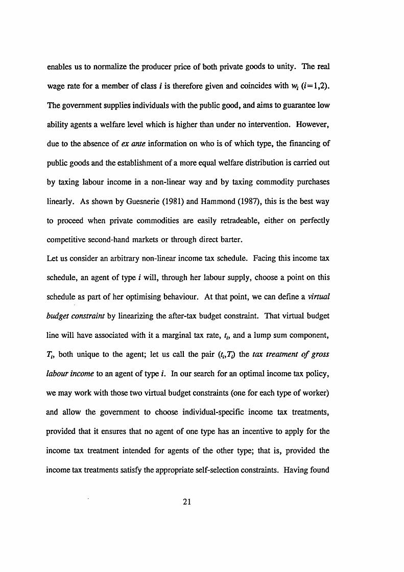
Facing the income tax treatment (/,-, 7]) and the marginal commodity tax rates ja and

Tb, an individual of type i solves the following problem:

where qa and qb stand for the consumer prices of commodities a and b, resp., which

are equal to the producer prices plus the commodity taxes (viz qc= l + T c, c —a,b).

Because profit income is zero, any feasible allocation in this economy which is

implemented by a fiscal policy can also be implemented by means of a modified

fiscal policy with one of the commodity tax rates normalized to zero. We will

choose 7 b = 0 and henceforth commodity b shall be referred to as the numeraire.

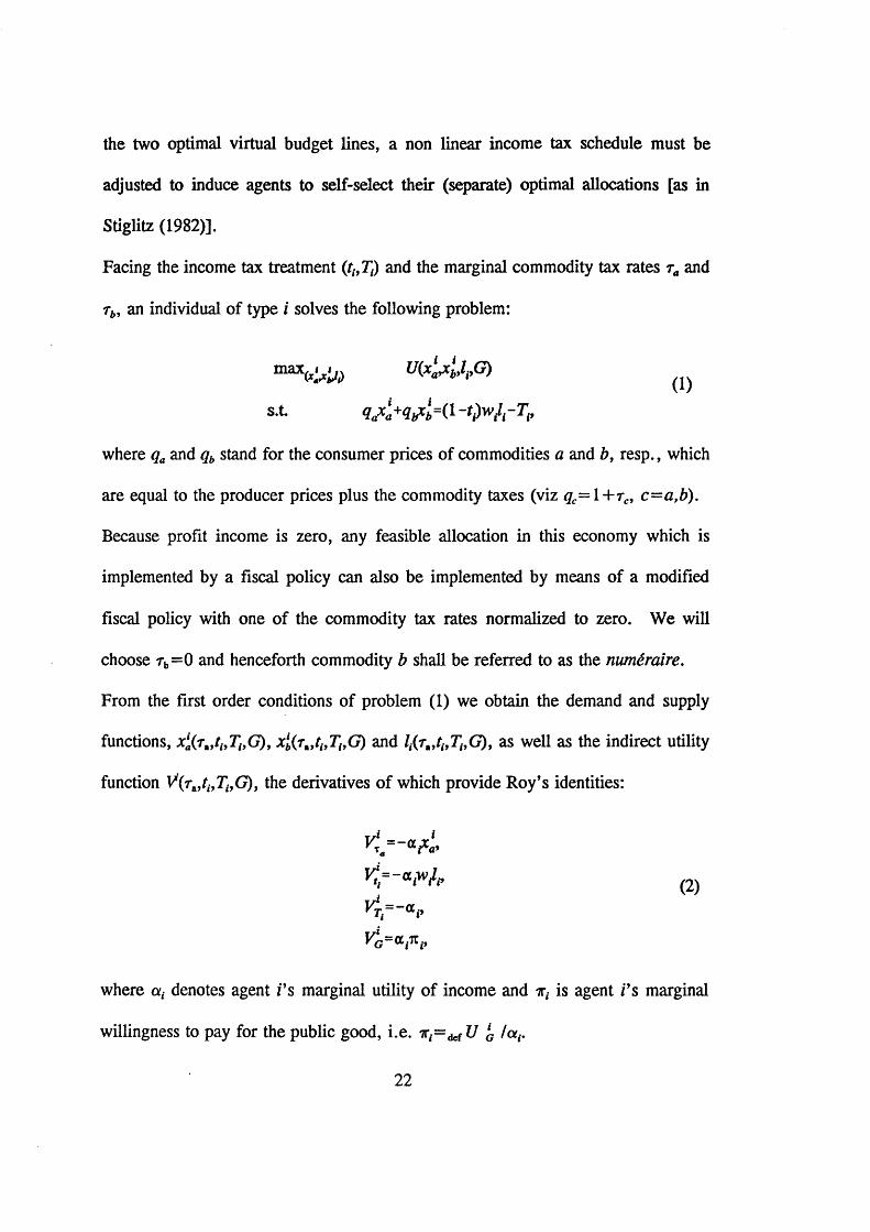
From the first order conditions of problem (1) we obtain the demand and supply

functions, x la(T„thTi9G), x lb(T„thTiyG) and /,(r,,r£,7 .,G), as well as the indirect utility

function V(rA,tiyTiyG)y the derivatives of which provide Roy’s identities:

where at denotes agent z’s marginal utility of income and is agent Vs marginal

willingness to pay for the public good, i.e. 7 = ^ U lG /at.

max, < j(i)

T /• *

K =~atw^vL=-rr

(2)

Let us now inquire about the maximal utility level an agent of type 2 would derive

when applying for the income tax treatment {tx,Tx) designed for type 1 agents, and

how this utility level is affected by reforms in the fiscal and expenditure policy.

Since the gross income of a type 1 individual is given by wxlx, agent 2, in order to

mimic the pre-tax income of individual 1 , must supply a quantity of labour J2—

wlll/w2 (henceforth, all variables pertaining to the mimicker will be written with an

upper bar). With this amount of foregone leisure, the mimicking agent maximizes

her utility with respect to xa and xb within the limits of the net disposable income (1-

t\)W\l\-Tx. The resulting demand functions are given by ^f(ra,r1, r 1,G;/2) and

x2b(TaA>Tx,G;l2); they imply the indirect utility function

(3)

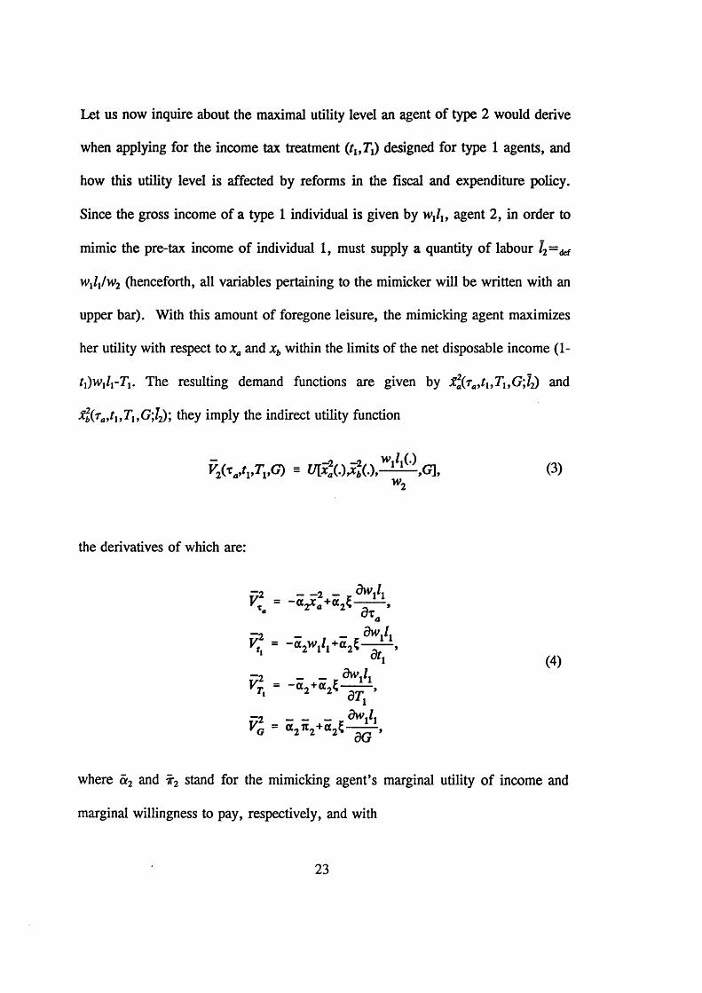
the derivatives of which are:

(4)

where a2 and x2 stand for the mimicking agent’s marginal utility of income and

marginal willingness to pay, respectively, and with

defJ a2w2

denoting the difference between the implicit marginal income tax rate which induces

the mimicker to provide 12 hours of labour (1 + Ujlaw^) and the nominal tax rate

Because the mimicker is forced to supply her labour at an exogenously determined

suboptimal level (viz. wJi/w2), £ will in general be different from zero. In appendix

A it is shown that assumption N is sufficient for £ to be positive. Decentralization

requires that the utility level implied by (3) does not exceed the utility level

^(Ta,t29T2tG).

Let us now turn to the government’s problem. It chooses a fiscal and expenditure

policy which makes high productivity agents as well off as possible, while at the

same time providing low productivity agents with a standard of living V\ above their

welfare level under no intervention, and keeping its budget in balance. In other

words, it solves

max(Vi,r,,G) ^ 2(Ta»2» 2» ^

s.t. V \ t j v Tv G) ;> u] (v.)

^ ( V ^ G ) * (y) (6)w2

+ «2[ v £ ( ') +f2w2/2( )+r2] a G (A.)

The first constraint is the standard of living condition on low ability agents and the

third constraint ensures a balanced government budget; the associated Lagrange

24

multipliers are /* and X, resp., and both will be positive due to monotonicity of

preferences. The second constraint is the self-selection condition on high ability

agents. Its associated Lagrange multiplier 7 will take on a strictly positive value

when the redistributional aim of the government (i.e. t/1) is sufficiently high. 2

Manipulation of the first order conditions to problem (6 ) with respect to tu Tu t2,

T2 and G results in the following system of equations:3

2 A similar self-selection constraint imposing that an agent of type 1, when masquerading as a type 2 person, should not be able to derive a higher utility level than when applying for the income tax regime intended for type 1 , has been left out. First because under assumption N, at most one self-selection constraint will be binding. And second, because the government aims at guaranteeing type 1 agents a higher living-standard than under no intervention, the income tax treatment for this class will be relatively favourable, and therefore members of that class will never have any incentive to dissemble as high ability agents. (This is what Stiglitz (1982) refers to as the "normal" case.)

3 To derive these conditions we first obtain the first order conditions (foe) of (6 ), by equating to zero the derivatives of the associated Lagrangian w.r.t. the six decision variables. Next, we perform the following standard manipulations: (i): foc(tl)-wlll • fo c ^ ) =0; (z7) foc(t2)-w2l2*foc(T^)—0; (iii) foc(rJ-xi• foc(r,)-xi • f o c ^ =0; and (zv) foe(G)+ • foc(Ti)+ ir2 • foc(T2) =0. (7a) and (7b) then follow by simple rearrangement of (i) and (zi), resp.. (7c) and (7d) are obtained by substituting tx and t2 in {iii) and (zv) for the RHS’s of expressions (7a) and (7b) and rearranging.

25

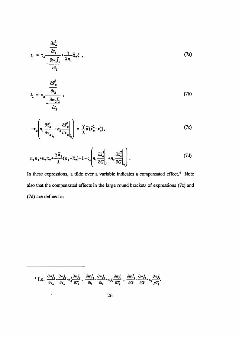
In these expressions, a tilde over a variable indicates a compensated effect. 4 Note

also that the compensated effects in the large round brackets of expressions (7c) and

(7d) are defined as

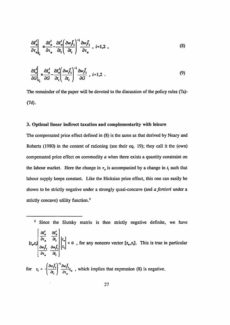
a xn 3x‘a d x j dW'1,)1 dW'I,(8)

(9)

The remainder of the paper will be devoted to the discussion of the policy rules (7a)-

3. Optimal linear indirect taxation and complementarity with leisure

The compensated price effect defined in (8) is the same as that derived by Neary and

Roberts (1980) in the context of rationing (see their eq. 19); they call it the (own)

compensated price effect on commodity a when there exists a quantity constraint on

the labour market. Here the change in ra is accompanied by a change in t{ such that

labour supply keeps constant. Like the Hicksian price effect, this one can easily be

shown to be strictly negative under a strongly quasi-concave (and a fortiori under a

strictly concave) utility function.5

5 Since the Slutsky matrix is then strictly negative definite, we have

(?d).

< 0 , for any nonzero vector [z^zj. This is true in particulard w f dw lt [*,•

for z. = ■za , which implies that expression (8) is negative.

27

Accordingly, by (7c), the optimal commodity tax rate, ra, has the same sign as (jt\-

*1), which denotes the amount of commodity a which the mimicking type 2 agent

consumes in excess of a type 1 agent. Since both agents earn the same gross income,

they will also be left with the same amount of disposable income. On the other hand,

the mimicking agent (being endowed with a higher ability) will be left with a larger

amount of leisure than a type 1 agent, and this may induce her to allocate her

disposable income in a different way. This suggests the use of the following

Definition: Assume both an exogenous amount o f disposable income and leisure are allocated to a consumer. A commodity is then said to be an l-complement (l- substitute) with leisure when that commodity is consumed in a larger (smaller) amount as more leisure becomes available.

Using the tools in Neary and Roberts (1980) it is possible to relate this commodity

classification to standard income and substitution effects. In appendix B it is shown

that commodity a is an 1-complement (substitute) with leisure if and only if individual

preferences yield income and cross substitution effects which are related in the

following way (cf eq B7):

dx dxh dx. d i /im— h- <(>) - ± —± . (1 0 )dT dt dT dt

In view of the homogeneity restriction {qa • dXaldt+dXbldt+ uja 'dl/dt= 0), it is not

difficult to conclude from (10) that, together with normality of both commodities,

Hicksian complementarity of commodity a with leisure (dXa/d t> 0) is a sufficient

28

condition for this commodity to be an 1-complement with leisure.6

With the definition of 1-complementarity in mind, our first results can be stated as

follows:

Proposition 1: The tax on commodity a will be positive (negative) whenevercommodity a is an l-complement (l-substitute) with leisure.

Corollary 1: When commodity a is a Hicksian complement with leisure and with both private commodities being normal goods, ra will be positive.

As mentioned in the introduction, Atkinson and Stiglitz (1976) studied the case in

which marginal commodity taxes may vary across both commodities and individuals

(whereas we assume they may differ only across commodities). They conclude that

no commodity taxes should be imposed on the high productivity person while those

imposed on the low productivity one should vary across commodities according to

their complementarity with leisure (there, complementarity is to be understood as the

extent to which the marginal willingness to pay for a commodity increases with

leisure). Whence, a sufficient condition for commodity taxation to vanish is weak

6 From (10), it is also clear that a necessary and sufficient condition for good a to be 1-independent with leisure is

dx dxa dx, dx. . dxa etc dx. dx. £/__£n-1 _ __£/__£\-l £/_£\-l ___£/__£\-ldt dT dt dT dt dT dt dT

with the ratio’s in the expression to the left of the equivalence sign denoting the change in T required to restore commodity demand to its original level after an marginal increase in t.

29

separability in the utility function between leisure on the one hand and commodities

on the other. A fortiori, the same condition remains sufficient when commodity tax

rates are constrained to be uniform across agents. Indeed, when commodities are

weakly separable from leisure, the allocation of disposable income over these

commodities will be independent of the amount of leisure, and therefore xj=xj,

implying r ,= 0.

For an economy with a continuum of types, Christiansen (1984) inquires about the

desirability to introduce uniform marginal commodity taxes when an optimal income

tax is in place. He finds that the introduction of a commodity tax (subsidy) will

entail a welfare improvement when that commodity is "negatively (positively) related

to labour", a commodity classification which precisely coincides with our 1-

complementarity (1-substitutability). In this respect, Proposition 1 is an obvious

translation of the rules derived by Christiansen (1984) and Tuomala (1990) to a two-

class economy. The advantage, however, of the present framework is that the

optimal tax formula (7c) can be given a transparent cost-benefit interpretation.

First, note that taxing a good which is an 1-complement with leisure relaxes the self­

selection constraint: this effect is caught by the RHS of (7c). To see this, let us rise

r. by At. (>0) and simultaneously reduce 7j by ATi=-x[ATt (/=1,2). These reforms

do not affect the utility of either type of non-mimicking individuals; the mimicker is

however worse off. To keep her at the same level of satisfaction would require a

lump sum tax rebate of x^Ar,; so her utility falls by a(jtJ-xl)Art, thereby relaxing the

self-selection constraint. However, raising r. causes further distortions in the price

30

system; its effect on the deadweight loss is caught by the LHS of (7c).

The explanation for the use of a labour constrained substitution effect in the

measurement of the deadweight loss is the following. What the non-linear income

tax schedule does in the quantity space [as in Stiglitz (1982)] is to make two distinct

combinations of gross and disposable income available. (As a matter of fact, the

virtual budget constraints, together with the self selection constraint exactly replicate

this.) Any agent may select any of these combinations, but the choice is clearly a

non-marginal one. The presence of the labour constrained substitution effects on the

LHS of (7c) indicates that, as the indirect tax system is marginally changed, the agent

is unable to respond to this change by a marginal adjustment of her labour supply

(and hence of her gross income). Consequently, the resulting reallocation of her full

disposable income will be as if a quantity constraint on labour supply applies.

Therefore, formula (7c) yields the optimal trade-off between the level of deadweight

loss and the relaxation of the self-selection constraint, and focuses on commodity a

only.

Finally, it is interesting to compare our commodity tax rule with the one provided by

Mirrlees (1975, eq 9). In that paper, Mirrlees shows that in a two class economy

where a fully linear tax system is operated, Pareto efficiency requires the following

equalities to hold (in our notation, and with the uniform marginal income tax denoted

by t):

31

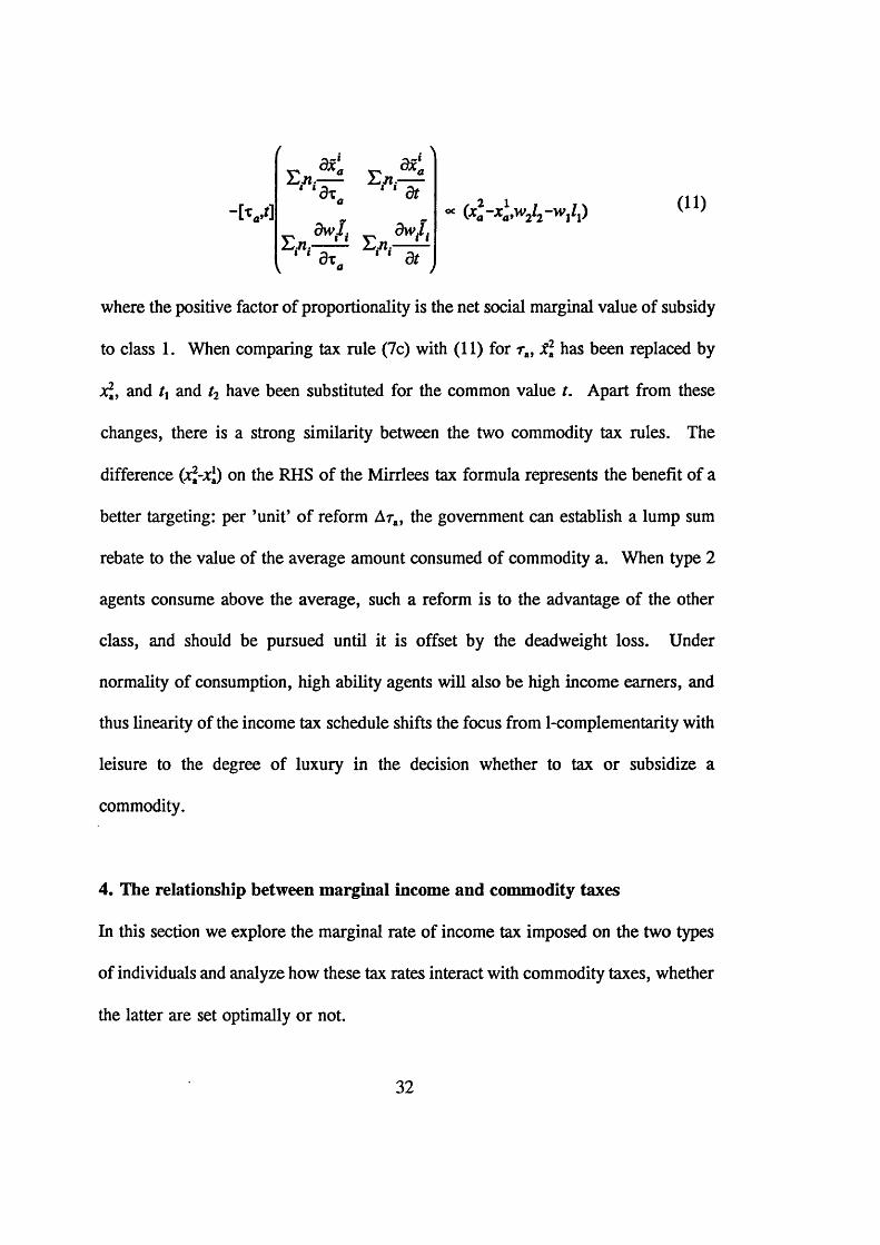
-[ V S

K r a ? ' 'L n . h n :----3*. 1 ‘ dta

1 ' 3t„ ' ' 3f<*

(11)

where the positive factor of proportionality is the net social marginal value of subsidy

to class 1. When comparing tax rule (7c) with (11) for ra, x\ has been replaced by

xj, and tx and t2 have been substituted for the common value t. Apart from these

changes, there is a strong similarity between the two commodity tax rules. The

difference (xj-xj) on the RHS of the Mirrlees tax formula represents the benefit of a

better targeting: per ’unit’ of reform Ara, the government can establish a lump sum

rebate to the value of the average amount consumed of commodity a. When type 2

agents consume above the average, such a reform is to the advantage of the other

class, and should be pursued until it is offset by the deadweight loss. Under

normality of consumption, high ability agents will also be high income earners, and

thus linearity of the income tax schedule shifts the focus from 1-complementarity with

leisure to the degree of luxury in the decision whether to tax or subsidize a

commodity.

4. The relationship between marginal income and commodity taxes

In this section we explore the marginal rate of income tax imposed on the two types

of individuals and analyze how these tax rates interact with commodity taxes, whether

the latter are set optimally or not.

32

Let us first look closer into the marginal income tax rate to which high ability types

are subjected. As pointed out by Tuomala (1990, p 175) and Edwards et al (1994),

it is a property of the optimal tax system that the total tax liability of an high ability

individual should remain unaffected by a marginal increase in this individual’s labour

earnings.7 An equivalent interpretation would be that the government does not

collect any extra tax revenue when augmenting the marginal income tax rate in a

compensated way (i.e. by appropriately adjusting the lump sum tax treatment); this

is easy to see by rewriting (7b) as re• b^Jbt2 + t2*dw2Vdt2 =0.

According to Stiglitz (1982), no marginal tax ought to be imposed on the labour

income of the high ability agent, when direct and indirect taxes can both be non­

linear. Note that in our setting, the same result (t2=0) applies if the agents’ utility

functions are weakly separable between all consumption goods and leisure. No

commodity taxes are then required, which implies that t2=0 from (7b).

In general, however, a non-zero marginal income tax at the top is motivated by the

existence of efficiency losses created by indirect taxation. Distortionary income

taxation (or subsidization) will be desirable to the extent that it offsets these efficiency

losses. Let us inquire how marginal income taxes should be set. As the denominator

on the RHS (7b) is always positive, we infer that t2 is positive or negative according

to whether the signs of the commodity tax on good a and that of the cross substitution

effect dX2Jdt2 are identical or opposite.

Assume without loss of generality that ra>0. If good a is a substitute for leisure in

7 Edwards et al (1994) speak of a zero effective marginal tax rate.

33

the Hicks sense (d&Jdt2< 0), it becomes optimal to subsidize high ability agents*

labour income at the margin (t2 < 0). Such subsidization tends to decrease leisure and

consequently more of good a will be demanded. Whence, t2 is chosen in such a way

that its effect on counteracts that of the commodity tax on good a. On the other

hand, when good a is a complement for leisure in the Hicks sense (d;?Jdt2>0), t2 will

take on a positive sign. Taxation of income at the margin tends to increase leisure

and consequently more of good a will be demanded. Once again the effects of

income and commodity taxes on oppose each other. (With the appropriate changes

in sign the same kind of conclusions can be reached when the consumption of good

a is subsidized.) Note that those conclusions hold irrespective of whether Ta>0 is

optimal.

When also the commodity tax policy is part of the optimization exercise, we know

that the direction in which this policy should distort commodity demand is controlled

by the commodity’s degree of 1-complementarity with leisure. Hence the following

result:

Proposition 2: Under a Pareto efficient fiscal policy, the marginal tax on the income o f the high productivity individual has the same (opposite) sign as that on commodity a as long as leisure and good a are complements (substitutes) in the Hicks sense.

Corollary 2: When commodity a is a Hicksian complement with leisure, and with both private commodities being normal goods, t2> 0.

Let us now focus on the optimality condition w.r.t. tx. From condition (7a), it

34

transpires that distortive taxation of low incomes is motivated by two reasons. The

standard reason, accounted for by the second RHS term in (7a), is that it mitigates

the incentive of high ability agents to masquerade as low ability ones. But as we

have argued in the previous section, this motivation also underlies the indirect tax

policy. Because this policy distorts the decisions of low ability agents to purchase

commodity a, the alleviation of the ensuing efficiency losses provides a second

rationale for distortive taxation of low incomes. Of course, in the absence of

commodity taxes, such efficiency losses are zero, and tl is positive for the standard

reason.

Let us now turn to the sign of tx and make the following rather weak assumption:

Assumption I: The sign o f the compensated marginal income tax effect on the demand for commodity a is independent o f the income level.

Because under this hypothesis the first term on RHS of (7a) has the same sign as the

RHS of (7b) and because the second term is positive under the normality assumption

N, tx > 0 is a necessary condition for t2 > 0. Under an optimal commodity tax policy,

the same conditions of corollary 2 which are sufficient to have tj> 0 are also

sufficient for ^ > 0 . On the other hand, the simultaneous occurrence of marginal

income taxation of low ability persons (tx > 0) with marginal income subsidization of

high ability persons (t2 < 0) cannot be ruled out a priori. But this requires commodity

a to have an opposite preference characterization in the two senses. Under normality

of both commodities, the only opposite characterization possible is Hicksian

substitutability and /-complementarity with leisure, which is therefore a necessary

condition on preferences for income subsidization of low ability types (tx < 0) to be

optimal. Our findings in this section are summarized in the following proposition and

its corollary.

Proposition 3: Under a Pareto efficient fiscal policy, tx> 0 is a necessary condition for t2> 0.

Corollary 3: Under normality o f both commodities, a necessary condition fo r t, < 0 to be optimal is that commodity a is both a Hicksian substitute and an l-complement with leisure.

5. The Samuelson rule with non-linear income and linear commodity taxes In this section we interpret the modified Samuelson rule as given by expression (7d).

This expression holds even if the commodity tax is not set at its optimal level. For

the sake of interpretation let us consider first the case in which no commodity taxes

are levied (ra=0). Under this (possibly Pareto inferior) indirect tax policy, the RHS

of (7d) reduces to unity, generating the modified Samuelson rule derived by Boadway

and Keen (1993). The modification is due to the presence of the term ya 2(Ti-T^)l\

which accounts for the impact the public expenditure policy may have on the self­

selection constraint. If the mimicker has the same marginal willingness to pay for

the public good as individual 1, the standard Samuelson rule obtains (7z1x1+n2T2:=l),

even though public expenditure is financed through distortive (non-linear) income

taxation.

36

Again, a transparent cost-benefit interpretation can be provided. Suppose that

initially the planner chose public expenditure according to the standard Samuelson

rule. Let us then rise G by one unit and at the same time increase Tx and T2 by t x

and x2 respectively (AG=1, ATl=irl and Ar2= x 2). These budget-balancing changes

keep both individuals 1 and 2 on their original indifference curves, but they will

affect the utility of the mimicking agent (and therefore the self selection constraint)

to the extent that xr x2 is different from zero. Consider, for instance, the case where

x2< xx. Then under this hypothetical policy reform the mimicker is made worse off

since Tx rises by more than she is willing to pay for. In this case, the self selection

is relaxed by expanding public good provision and formula (7d) (with the RHS = 1)

indicates that the public good ought to be provided at a level where the aggregate

marginal willingness to pay falls short o f the marginal cost (cf proposition 1 of

Boadway & Keen, 1993). Thus with x25*xj, the public expenditure policy affects

the income transfer policy through its effect on the self-selection constraint. A case

where such an effect will not occur is where the agents’ utility functions are weakly

separable between all private and public goods (taken together) and leisure, i.e.

U(xa,xb,l,G)=u[F(xajcb,G),l\. Then the marginal willingness to pay for the public

good is the same for all agents consuming the same commodity bundle, even when

they supply a different amount of labour (in particular x ^ x * ). In that case, the

standard Samuelson rule for public good provision continues to apply (cf Boadway

& Keen, 1993, Corollary 1). The above results hold even with zero indirect

taxes not being optimal. In the case where these taxes differ from zero, equation (7d)

37

can be given the same interpretation as in the case without indirect taxes except that

the impact on indirect tax revenue of a change in G needs to be accounted for as

well. This is done through the compensated effects on consumption decisions of the

change in G. Note, however, that as in section 3 the labour supply (and therefore

gross income) of both types of individuals kept constant by means of simultaneous

changes in f, and t2 (see eq 9).

It is interesting to compare our modified Samuelson formula with the one obtained

by Atkinson and Stem (1974) for the case where (linear) commodity taxes and an

optimal linear income tax are used. As reported in Atkinson and Stiglitz (1980) it

can be written as:

n1TZ1+n2TZ2+(n1 +n2)cov(bi,T:i)=l -x tdxa dxa

n, +tin----1 dG ^dG

(12)

where bt is the net social marginal valuation of individual i’s income, viz. b ^ a fk -

T^bxiJdTi. Thus, under optimal linear income taxation, the distribution covariance

term focuses on the way the willingness to pay for the public good is related to bt and

hence to income. Under optimal wo/i-linear income taxation, the equivalent term

rather focuses on the relationship between the willingness to pay and available

leisure. In addition, the terms accounting for the effect on tax revenues of the change

in G in formulas (7d) and (12) are somewhat different since the former involves the

impact on tax revenue of the changes in tx and t2 required to keep lx and l2 constant.

We can now wonder under which circumstances our modified Samuelson rule reduces

to the standard rule if the indirect tax parameters are set optimally. From section 3

38

we know that if the utility function is weakly separable between labour and all private

consumption goods (taken together), then no commodity taxation need be employed.

Both the utility functions U[F(xarxb),G,l] and U[F(xayxb,G),l] meet this requirement;

they will both make commodity taxation redundant. While the latter function also

makes 7r2=7ri (see earlier), the former does not, in which case mitigating effects on

the self-selection constraint will affect public goods provision as well. With

preferences representable by the latter utility function, neither indirect taxation nor

the provision of the public good will give rise to such mitigating effects, so that the

level at which the public good should be supplied is to be derived from the standard

Samuelson rule:8

Proposition 4: Under a Pareto-efficient indirect and direct tax policy, a sufficient condition for the standard Samuelson formula to apply is that the agent's utility functions are weakly separable between leisure and all private and public goods taken together.

6. Concluding comments

In this paper we enquired about Pareto efficient fiscal and public expenditure policies

for a discrete class economy where the government cannot directly observe the

individuals’ abilities and where indirect tax rates are constrained to be uniform across

individuals for reasons of arbitrage. By assuming a high and low ability class, and

8 Proposition 1 and Proposition 2 of Christiansen {1981) give, with reference to the continuum case, a result similar to our Proposition 4.

39

by restricting the number of private commodities to two, the problem has been

formulated in the simplest possible way.

As far as the optimal tax policy is concerned, two conclusions have been derived.

First, we showed that if a good is more complementary with leisure than the

numeraire, it should be taxed at a higher rate at the margin. Second, a marginal

increase of the respective marginal income tax should result in a zero tax extraction

from the high ability individual and positive extraction for the low ability individual.

These are results which are consistent with the existing literature and economic

intuition.

However we also showed that the value of the optimal marginal income tax rate on

high incomes is chosen so as to partially offset the efficiency losses from indirect

taxation. This leads to a synergy between the marginal income tax rate and the

commodity tax rate, in that the former should be chosen so as to counteract the

effects of the latter on consumption decisions. In particular we identified Hicksian

complementarity of the non-numeraire commodity with leisure together with

normality of both private goods as sufficient conditions for a positive indirect tax rate

and a positive marginal tax rate on high incomes to obtain. Besides its potential for

relaxing the self-selection constraint, the marginal income tax rate on low incomes

is chosen for similar reasons of counteractions.

As to the optimal provision of public goods we put together two results of the

literature. The first appeared in Atkinson and Stem (1974) where a fully linear

income and commodity tax system is implemented, and the second in Boadway and

40

Keen (1993) where only non-linear income taxes are in force. We derived a modified

Samuelson formula for a hybrid tax structure. If the agents* utility function are

weakly separable between private and public goods (taken together) and leisure, the

standard Samuelson rule was shown to apply again.

41

Appendix A

Like in Christiansen (1984) we can consider the consumer’s problem as a two-stage process. In the second stage, the consumer allocates a net disposable income z, conditional upon the fact that a gross income wl has been earned by supplying / hours of labour. The solution to this problem may be inserted into the utility function to U( •) to provide a new utility function defined over z and /, u(z,l), which again shares all the desirable properties (the proof is analogous to the one given by Bronsard, 1983). In the first stage, the consumer then chooses values for z and I which maximize u(z,l) subject to the relationship between gross and net income as defined by the income tax schedule. In absolute value, the marginal rate of substitution in the (z,0-space is given by -w/mz>0. Whence, net disposable income z is a normal good if

-u,^ (AD z— > 0

a/

It is not too difficult to demonstrate that the normality assumption N in the text will precisely guarantee this.

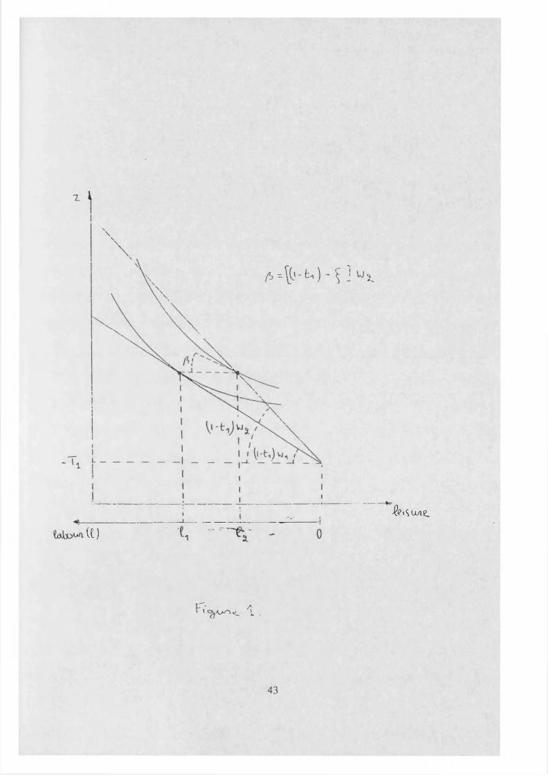
Suppose now that, facing the income tax treatment (tu Tj), the low ability agent chooses to supply lx hours of labour in the first stage. To apply for the same tax treatment, the high ability agent should supply only /2=w1/1/w2 hours of work. When the inequality (Al) is verified, this means that facing the income tax treatment (f,,7i), this agent would like to supply more than ^ hours (see figure 1). In other words, at the bundle (S\-t^wxlx-Tul^, the mimicking agent’s supply price for labour is lower than her market wage rate w2. Put differently, the implicit marginal tax rate inducing the mimicking agent to supply /2 hours exceeds tx.

42

$?»SUA£_

Vt)

C'* /i» l ^ j_

Appendix B

Consider a consumer who disposes of a lump sum income m, who faces the price qa for the non-numeraire commodity a, and who is forced to supply 1° hours of labour at a net wage rate w because of a quantity constraint on the labour market.The demand system under these circumstances of rationing can be written as x£(qa,(j),m;r) (k=a,b). If the unconstrained demand system written as xk( •) (k=a,b), the former system may be related to the latter in the following way: xrk(qa,u,m;r)=xk[qa,co° ,m +(u-u°)r] where o>° denotes the consumer’s reservation wage at which she would like to supply exactly 1° hours of labour.When the consumer is forced to supply an extra dl° hours of labour, the effect on the demand for commodity a can be shown to decompose into an income and a substitution effect:

(B l)dm dl°

which can be related to standard income and substitution effects (see Neary and Roberts, 1980):

<K = (B2)dm dm do) do dm

aoi - (B3>d r da da

with the standard effects evaluated at that parameters [^J,co°,m+(cj-aj0) /0].The homogeneity restriction on the consumer’s decisions, implies that

dxn dx, sia — 2 + — = 0, (B4)

do) dco do

thereby providing the following implicit definition of the reservation wage co°:

44

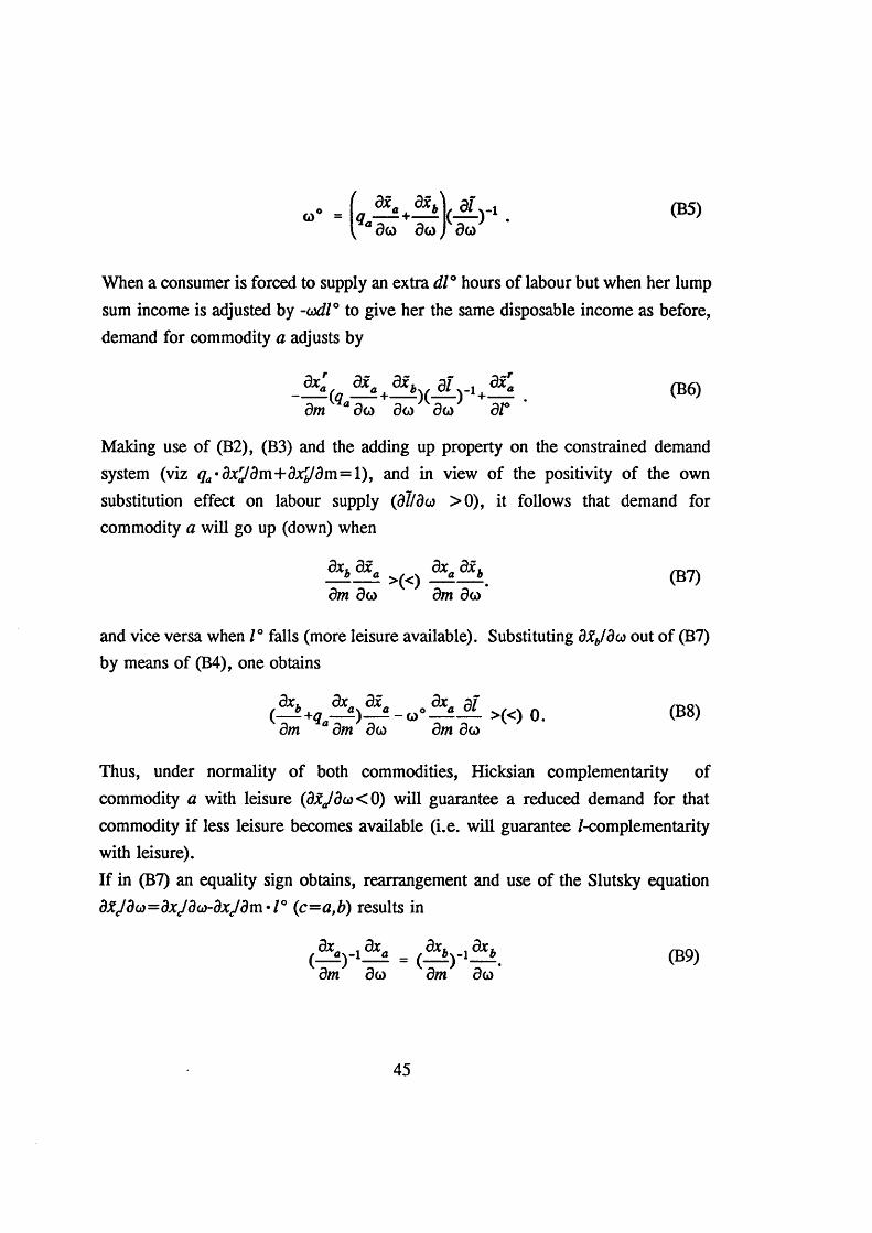
When a consumer is forced to supply an extra dl° hours of labour but when her lump sum income is adjusted by -ox//° to give her the same disposable income as before, demand for commodity a adjusts by

(B6)

Making use of (B2), (B3) and the adding up property on the constrained demand system (viz qa*8xrJ8 m+djt£/0m=l), and in view of the positivity of the own substitution effect on labour supply (81/do) >0), it follows that demand for commodity a will go up (down) when

and vice versa when /° falls (more leisure available). Substituting 8%b/8w out of (B7) by means of (B4), one obtains

Thus, under normality of both commodities, Hicksian complementarity of commodity a with leisure (8xjdo)<0) will guarantee a reduced demand for that commodity if less leisure becomes available (i.e. will guarantee /-complementarity with leisure).If in (B7) an equality sign obtains, rearrangement and use of the Slutsky equation 8XJ8o)=dxjd u-dxjd m • / ° (c=a,b) results in

dxb dxi- >(<)

3 * 0 5xb (B7)dm do dm 0o>

(B8)

References

Atkinson, A.B. and N.H. Stem, 1974, "Pigou, taxation and public goods", Review o f Economic Studies 41, 119-128.

Atkinson, A.B. and J.E. Stiglitz, 1976, "The design of tax structure: direct versus indirect taxation", Journal o f Public Economics 6, 55-75.

Atkinson, A.B. and J.E. Stiglitz, 1980, Lectures on Public Economics (McGraw-Hill: New York).

Boadway, R. and M.J. Keen, 1993, "Public goods, self-selection and optimal income taxation", International Economic Review 34, 463-78.

Bronsard, C., 1983, "From intertemporal strong quasi-concavity to temporary one", Economics Letters 12, 115-120.

Christiansen, V., 1981, "Evaluation of public projects under optimal taxation", Review o f Economic Studies 48, 447-457.

Christiansen, V., 1984, "Which commodity taxes should supplement the income tax?", Journal o f Public Economics 24, 195-220.

Edwards, J., M. Keen and M. Tuomala, 1994, "Income Tax, Commodity Taxes and Public Good Provision: a Brief Guide", Finanzarckiv, 472-487.

Guesnerie, R., 1981, ’On Taxation and Incentives: Further Reflexions on the Limits to Redistribution’, DP 89, Bonn University, forthcoming as Ch 1 in R. Guesnerie, A Contribution to the Theory o f Taxation (Cambridge: Cambridge University Press).

Hammond, P. J., 1987, ’Markets as Constraints: Multilateral Incentive Compatibility in a Continuum Economy’, Review o f Economic Studies 54, pp 399-412.

46

Mirrlees, J. A., 1975, "Optimal commodity taxation in a two class economy", Journal o f Public Economics 4, 27-33.

Nava, M., M. Marchand, and F. Schroyen, 1993, "Optimal taxation and provision of public goods with non-linear income and linear commodity taxes in a two class economy", CORE DP #9321.

Neary, P. and K. Roberts, 1980, "The theory of household behaviour under rationing", European Economic Review, 13, 25-42.

Pigou, A.C., 1947, A study in public finance, 3rd ed (Macmillan: London).

Samuelson, P.A., 1954, "The pure theory of public expenditure", Review o f Economics and Statistics 36, 387-389.

Stiglitz, J.E., 1982, "Self selection and pareto efficient taxation", Journal o f Public Economics 17, 213-240.

Tuomala, M., 1990, Optimal income tax and redistribution, (Clarendon Press: Oxford).

47

Chapter 2

DIRECT AND INDIRECT TAX EVASION: A SURVEY OF THE LITERATURE*

Mario Nava Center for Economic Performance

London School o f Economics

Abstract

The purpose of this selective survey of the literature on both income and commodity tax evasion is to show in which directions, the literature has evolved. Two main approaches are identified for both direct and indirect tax evasion literature.The so-called taxpayer’s point of view approach which is basically an exercise of maximization under uncertainty and the so-called tax collector’s point of view which is a refinement of the Mirrlees-Stiglitz approach to income taxation and of the Ramsey approach to commodity taxation. The current state of the art is such that both approaches share similar strengths and weaknesses.

* Thanks are due to Jonathan Leape who introduced me to the subject and helped with the revision of a first version and to all participants of the LSE PhD seminars 1993/94 for their comments. Comments from Tim Besley and Mick Keen have been very useful in polishing the final version. The usual disclaimers apply.

48

1. Introduction

After the excellent Frank Cowell (1990) review to write a survey about tax evasion

is a very hard job, at least for the next few years. The aim of this survey is just to

fill a possible gap in Cowell’s book. We present a comparative approach to the

literature on direct and indirect tax evasion. The literature on tax evasion is 22 years

old and contains roughly 210 papers. About 200 papers deal with direct tax evasion,

while the other 10 papers deal with indirect tax evasion. The difference in the number

of papers in the two areas is rather impressive and the topic of indirect tax evasion

seems to have been rather neglected in the last twenty years. However it is an area

of great theoretical and empirical importance especially in the European Union where

a greater harmonization of the system of indirect taxation is high on the agenda.

We will stress many similarities between the two literatures. Both in the direct and

indirect tax evasion literature one may find two different approaches. The taxpayer’s

perspective approach and the social perspective approach. We will comment on the

paper that we think to be the most representative in both approaches and in both

direct and indirect tax evasion literature. However, we will not give up the ambition

to supply the reader with an historical perspective. Actually the four chosen papers

in addition to being the most representative of their respective stream of literature,

are the first on each topic.

The problem of tax avoidance is left out of this essay and we shall make clear the

difference between tax evasion and tax avoidance. From a legalistic point of view

49

"avoidance" means to avoid tax legally, i.e. following the suggestions of a clever tax

adviser in filling in the tax declaration, while "evasion" means to avoid tax illegally

via e.g. under reporting. From an economic point of view, which concerns us more,

if the taxpayer practices "tax avoidance" he1 will stay in a world of certainty about

his post tax income; if he practices "tax evasion" he will shift in the world of

uncertainty: his actual post tax income will depend on the event of being checked and

recognized as tax evader which is an event having probability p ( 0 < p < l ) . The

evader takes decisions under uncertainty. These two definitions may lead an

economist and a lawyer to think differently about the same action. If there exists a

kind of tax evasion with no probability of being caught, for an economist this is just

tax avoidance and for a lawyer this is tax evasion. One could argue that evasion with

no probability of being caught is tax evasion also from an economic point of view,

but it is just a type of tax evasion not represented in the existing models.

Nevertheless a rational taxpayer would never comply with the law if tax evasion were

risk-free. Therefore in order to include the risk-free tax evasion in a model of

rational behaviour one need to reshape the standard notion of rationality. In other

words under the standard notion of rationality individual’s integrity depends on

individual’s risk aversion. However for our purposes the economic definition is the

one to keep in mind.

1 Since we are speaking about cheaters and since we are willing to describe models having a strong empirical validity, all cheaters are thought to be ..men!

50

The plan of the paper is as follows. In Section 2 we look at the famous and seminal

Allingham and Sandmo (1972) (taxpayer’s perspective approach to direct tax evasion)

and at Sandmo (1981) (social perspective approach to direct tax evasion). In Section

3, we will focus on the papers of Marrelli (1984) (taxpayer’s perspective approach

to indirect tax evasion) and Cremer and Gahvari (1993) (social perspective approach

to indirect tax evasion). Section 4 concludes.

2. Direct Tax Evasion

In this section we will present two well-known papers on income tax evasion. The

first one is the first article ever appeared in the literature on tax evasion and it adopts

the taxpayer’s perspective approach. The second one adopts the social perspective

approach.

2.1 The Taxpayer's Perspective Approach and Direct Tax Evasion

Just looking at the few references of Allingham and Sandmo (1972), one immediately

realizes why it is unanimously considered the path-breaking article on tax evasion:

there is no previous paper dealing with this topic with the exception of a mimeo by

Mirrlees, quoted in their footnote 1, which suggested theoretical investigation of the

matter. Their paper takes into account only the possibility of income tax evasion and

connects two different approaches: on one hand the so-called economics of criminal

activity (Becker 1968) on the other hand the analysis of optimal portfolio and risk

insurance (Arrow (1^70), Mossin (1968a, 1968b) and Stiglitz (1969). Tax evasion is

51

regarded as a matter of risk bearing and the paper provides the analytical background

for most of the following papers on the subject. We will see that many ideas

developed in later articles were already present in Allingham and Sandmo.

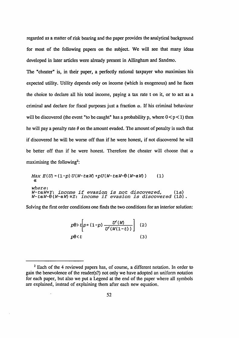
The "cheater" is, in their paper, a perfectly rational taxpayer who maximises his

expected utility. Utility depends only on income (which is exogenous) and he faces

the choice to declare all his total income, paying a tax rate t on it, or to act as a

criminal and declare for fiscal purposes just a fraction a. If his criminal behaviour

will be discovered (the event "to be caught" has a probability p, where 0 < p < 1) then

he will pay a penalty rate 0 on the amount evaded. The amount of penalty is such that

if discovered he will be worse off than if he were honest, if not discovered he will

be better off than if he were honest. Therefore the cheater will choose that a

maximising the following2:

Max E(U) =( 1 - p ) U(W-taW) +pU(W-taW-Q(W-aW) ) (1)a

w h e r e :W-taW=Y: in c o m e i f e v a s i o n i s n o t d i s c o v e r e d , ( la )W-taW-Q (W-aW) =Z: in c o m e i f e v a s i o n i s d i s c o v e r e d ( l b ) .

Solving the first order conditions one finds the two conditions for an interior solution:

U'(W)p0> t p + { l - p ) —T V i

( 2 )U'(W( 1 - t ) )

p0< t (3)

2 Each of the 4 reviewed papers has, of course, a different notation. In order to gain the benevolence of the reader(s?) not only we have adopted an uniform notation for each paper, but also we put a Legend at the end of the paper where all symbols are explained, instead of explaining them after each new equation.

52

Since the RHS of Eq. (2) is at most equal to the RHS of Eq. (3) and since both are

positive there is an interval of positive parameter values which will guarantee an

interior solution. Eq. (3) is readily interpretable: the taxpayer is a tax evader only in

the case that the expected penalty rate is less than the tax rate. The fraction in Eq.

(2) gives the decrease in marginal utility (so the gain in utility) from not paying taxes

honestly (e.g. [U'(W)/U'(W(l-t))]=0.5 means that your post tax marginal utility is

double than your pre-tax marginal utility): clearly, as higher is W as closer the

fraction is to 1 (keeping t constant). This means that the interval for partial evasion

is smaller for "richer" (or large firms) than for "poorer" (or small firms), so it could

be concluded that poorer are more likely to evade. But we shall come back to it later.

If the taxpayer cares not only about money but also about reputation (as hopefully

everyone does) the utility function should be modified to include reputation in state

0 (evasion but no detection, income Y) and state 1 (evasion and detection, income Z).

Again note that this individual is not worried about the fact of being honest or not,

but just about the fact of being recognized as a honest man or not. The best state for

him is being dishonest faking of being honest. A very vulgar man. The taxpayer now

maximises:

Max E(U) = ( l - p ) U ( Y , s 0) + p U { Z , s 1) (4)a

Assuming U(Y, s 0) >U(Y, s x) one obtains, solving the first order conditions, the

equivalent condition to Eq. (3):

53

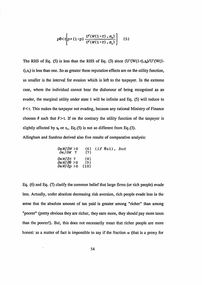
p 0 < t. U*(W(l- t) , s 0)

p + ( l - p ) — — ------ (5)r f i W i l - t ) ' S x)

The RHS of Eq. (5) is less than the RHS of Eq. (3) since (U’OV O-O^/U’OVO-

t),Sj) is less than one. So as greater these reputation effects are on the utility function,

as smaller is the interval for evasion which is left to the taxpayer. In the extreme

case, where the individual cannot bear the dishonour of being recognized as an

evader, the marginal utility under state 1 will be infinite and Eq. (5) will reduce to

6< t. This makes the taxpayer not evading, because any rational Ministry of Finance

chooses $ such that 0>t. If on the contrary the utility function of the taxpayer is

slightly affected by Sq or s,, Eq.(5) is not so different from Eq.(3).

Allingham and Sandmo derived also five results of comparative analysis:

daW/dW >0 (6) ( i f 0 ^ 1 ) , b u tda/dW ? (7)

d a W /d t ? (8)daW/dQ >0 (9)daW/dp >0 (10)

Eq. (6) and Eq. (7) clarify the common belief that large firms (or rich people) evade

less. Actually, under absolute decreasing risk aversion, rich people evade less in the

sense that the absolute amount of tax paid is greater among "richer" than among

"poorer" (pretty obvious they are richer, they earn more, they should pay more taxes

than the poorer!). But, this does not necessarily mean that richer people are more

honest: as a matter of fact is impossible to say if the fraction a (that is a proxy for

54

honesty) increases or decreases with income (Eq. 7), unless one makes assumptions

on the individual relative risk aversion.

The ambiguity on the sign of Eq. (8 ) depends upon the income and the substitution

effect: the income effect is positive, if more taxes are levied, the taxpayer is poorer

and under decreasing absolute risk aversion he reduces evasion; the substitution effect

is negative because an increase in tax rate makes more profitable, at the margin, to

evade.

Eq. (9) and Eq. (10) are intuitive and tied to the rationality of economic agents.

The paper ends with the analysis of the optimal behaviour of a forward looking

taxpayer in a dynamic setting. The crucial hypothesis is that if the taxpayer is

discovered as an evader he must pay a penalty, not only on taxes evaded in the

present year, but also on all he has evaded since the time when he last paid the full

amount. Therefore the rational taxpayer realizes that the today’s decision of cheating

must be influenced by past tax declarations (which determines the penalty) and in turn

it will influence the future. It can be shown that for this rational and forward looking

taxpayer even if it is possible to have an initial and partial evasion it will arrive a

time T from when on he will no more evade. This last result that, even if people are

not honest, but just rational, is possible to find a kind of penalty such that paying

taxes is optimal, is, in our opinion, extremely important.

Allingham and Sandmo (1972) treats the tax evasion issue as the individual choice of

utility maximisation under uncertainty, ’’...[they] explain to us how they choose to

fill in their income tax declaration" Kolm (1973). We do think that this approach is

55

extremely interesting from the individual point of view, but at the same time we do

agree with the comment of Kolm (1973): "But this is hardly public economics; in

fact, it is very private. What is really public economics is their tax collector’s

viewpoint."

A second stream of literature focuses on the "public economics" standpoint in the

sense of the above quoted Kolm’s sentence. The main reason for us to be concerned

with the social perspective lies in the peculiarity of fiscal frauds. A great majority of

other illegal activities involving money can be classified as acts against the law of

private property and generically an act against an individual or an institution. If I rob

a bank I am breaking the law which says that bank’s money are not mine or to a

larger extent that exists a right of private property over money that needs to be

respected. If I am evading taxes, e.g. simply not stating in my income tax declaration

part of my earnings, I am stealing money to Tax Collector Authority (the

Government). Being Government’s wealth made up of everyone’s contributions this

is an act against all fellow citizens and generically against the society. Analyzing tax

evasion seems therefore appropriate to take a social perspective standpoint and to see

how tax evasion affects government ability of raising taxes. As a matter of fact tax

evasion may be conceived both linked to some illegal activity (I live robbing banks

and I do not declare my earnings to the Tax Authorities) and linked to perfectly legal

activities (I run a shop and I underreport my revenues).

56

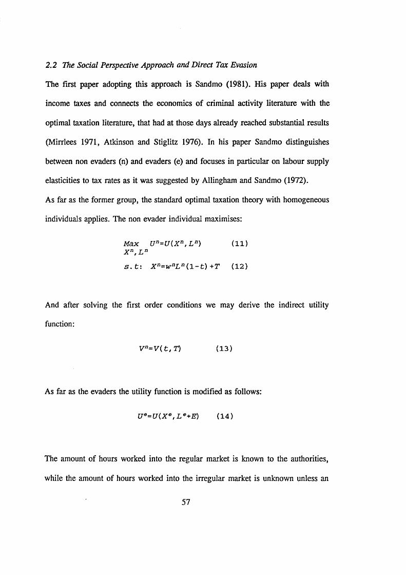
2.2 The Social Perspective Approach and Direct Tax Evasion

The first paper adopting this approach is Sandmo (1981). His paper deals with

income taxes and connects the economics of criminal activity literature with the

optimal taxation literature, that had at those days already reached substantial results

(Mirrlees 1971, Atkinson and Stiglitz 1976). In his paper Sandmo distinguishes

between non evaders (n) and evaders (e) and focuses in particular on labour supply

elasticities to tax rates as it was suggested by Allingham and Sandmo (1972).

As far as the former group, the standard optimal taxation theory with homogeneous

individuals applies. The non evader individual maximises:

Max Un=U(Xn, L n) (11)X n, L n

S. t : X n=wnL n ( l - t ) +T (12)

And after solving the first order conditions we may derive the indirect utility

function:

Vn= V { t , T ) (13)

As far as the evaders the utility function is modified as follows:

U6=U( X0, L e+E) (14)

The amount of hours worked into the regular market is known to the authorities,

while the amount of hours worked into the irregular market is unknown unless an

57

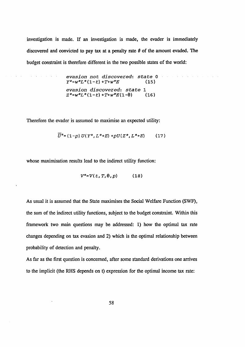
investigation is made. If an investigation is made, the evader is immediately

discovered and convicted to pay tax at a penalty rate $ of the amount evaded. The

budget constraint is therefore different in the two possible states of the world:

e v a s i o n n o t d i s c o v e r e d : s t a t e 0 Y e=weL e ( 1 - t ) +T+weE (15)

e v a s i o n d i s c o v e r e d : s t a t e 1 Z e=weL e ( 1 - t ) +T+weE ( l - Q ) (16)

Therefore the evader is assumed to maximise an expected utility:

Ue= ( l - p ) U ( Y e , L e+E) + p U( Ze , L e+E) (17)

whose maximisation results lead to the indirect utility function:

V6= V ( t , T , Q , p ) (18)

As usual it is assumed that the State maximises the Social Welfare Function (SWF),

the sum of the indirect utility functions, subject to the budget constraint. Within this

framework two main questions may be addressed: 1) how the optimal tax rate

changes depending on tax evasion and 2 ) which is the optimal relationship between

probability of detection and penalty.

As far as the first question is concerned, after some standard derivations one arrives

to the implicit (the RHS depends on t) expression for the optimal income tax rate:

58

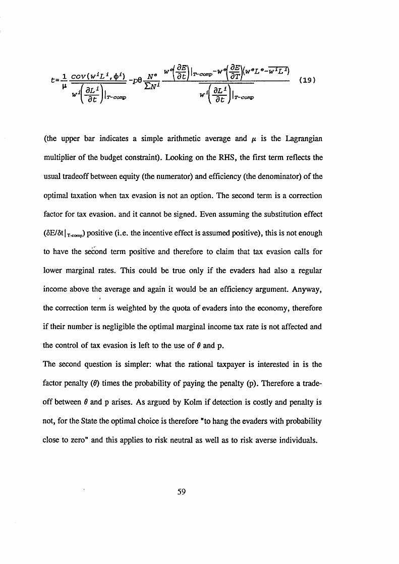
(the upper bar indicates a simple arithmetic average and n is the Lagrangian

multiplier of the budget constraint). Looking on the RHS, the first term reflects the

usual tradeoff between equity (the numerator) and efficiency (the denominator) of the

optimal taxation when tax evasion is not an option. The second term is a correction

factor for tax evasion, and it cannot be signed. Even assuming the substitution effect

(<5E/<5t | x^p) positive (i.e. the incentive effect is assumed positive), this is not enough

to have the second term positive and therefore to claim that tax evasion calls for

lower marginal rates. This could be true only if the evaders had also a regular

income above the average and again it would be an efficiency argument. Anyway,

the correction term is weighted by the quota of evaders into the economy, therefore

if their number is negligible the optimal marginal income tax rate is not affected and

the control of tax evasion is left to the use of $ and p.

The second question is simpler: what the rational taxpayer is interested in is the

factor penalty (0) times the probability of paying the penalty (p). Therefore a trade­

off between 0 and p arises. As argued by Kolm if detection is costly and penalty is

not, for the State the optimal choice is therefore "to hang the evaders with probability

close to zero" and this applies to risk neutral as well as to risk averse individuals.

These results are found under two strong ethical assumptions: utilitarianism of the

social welfare function and rational behaviour of individual. These assumptions

regarded as standard while dealing with normal goods and activities should be deeply

questioned when we are dealing with illegal activities.

When tax evasion is considered the final result is not robust to the choice of the

SWF. The Utilitarian Social Welfare function for example, if no incentive effect is

considered, allows for a decentralized self-redistribution such that tax evasion

increases the SWF if evaders have higher than average marginal utilities of income

(i.e . if they are the less well off). If there exists any incentive effect from the tax

reduction (i.e. tax evasion) it could also be the case that the SWF increases if

"skilled" people were allowed to evade. Allowing for efficiency arguments to play

a role in the shape of optimal taxation seems to open the door to accepting horizontal

inequality between evaders of similar income but with a different degree of tax

compliance. As argued above, in order not to allow efficiency to play a role one

needs to reshape the notion of rationality.

3. Indirect Tax Evasion

This section is constructed as the previous one. We will present two papers dealing

with indirect tax evasion having two different approaches. Marrelli (1984), the first

paper in the literature of indirect tax evasion, has the taxpayer’s perspective

approach, similarly to Allingham and Sandmo (1972). Cremer and Gahvari (1993),

has the social perspective approach, similarly to Sandmo (1981), and analyses how

60

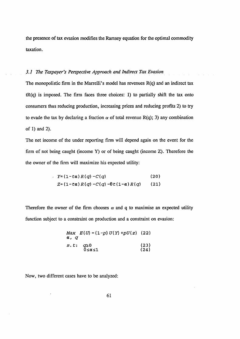
the presence of tax evasion modifies the Ramsey equation for the optimal commodity

taxation.

3.1 The Taxpayer's Perspective Approach and Indirect Tax Evasion

The monopolistic firm in the Marrelli’s model has revenues R(q) and an indirect tax

tR(q) is imposed. The firm faces three choices: 1) to partially shift the tax onto

consumers thus reducing production, increasing prices and reducing profits 2 ) to try

to evade the tax by declaring a fraction a of total revenue R(q); 3) any combination

of 1) and 2 ).

The net income of the under reporting firm will depend again on the event for the

firm of not being caught (income Y) or of being caught (income Z). Therefore the

the owner of the firm will maximize his expected utility:

. Y = ( l - t a ) R ( q ) - C { q ) (20)

Z = ( l - t a ) R ( q ) - C ( q ) - 0 t ( l - a ) R { q ) (21)

Therefore the owner of the firm chooses a and q to maximise an expected utility

function subject to a constraint on production and a constraint on evasion:

Max E { U ) = ( l - p ) U { Y ) + p U { z ) (22)a , q

s . t : qzO (23)O s a s l (24)

Now, two different cases have to be analyzed:

61

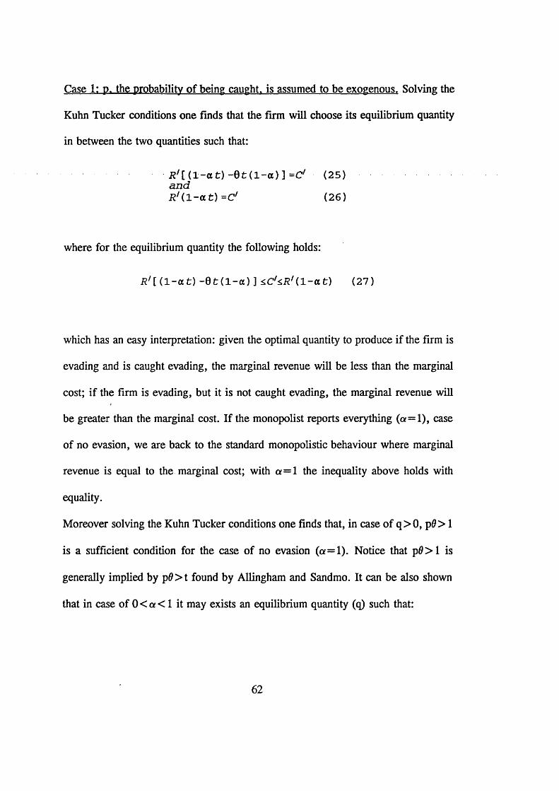
Case 1: p. the probability of being caught, is assumed to be exogenous. Solving the

Kuhn Tucker conditions one finds that the firm will choose its equilibrium quantity

in between the two quantities such that:

R ' i i l - a t ) - 0 f c ( 1 - a ) ] =C/ (25)a n dR1 ( 1 - a t ) -C' (26)

where for the equilibrium quantity the following holds:

^ [ ( 1 - a t ) - 0 1 (1 -a ) ] ^ C ^ f l ' U - a t ) (27)

which has an easy interpretation: given the optimal quantity to produce if the firm is

evading and is caught evading, the marginal revenue will be less than the marginal

cost; if the firm is evading, but it is not caught evading, the marginal revenue will

be greater than the marginal cost. If the monopolist reports everything (a = l) , case

of no evasion, we are back to the standard monopolistic behaviour where marginal

revenue is equal to the marginal cost; with a = l the inequality above holds with

equality.

Moreover solving the Kuhn Tucker conditions one finds that, in case of q> 0 , p0> 1

is a sufficient condition for the case of no evasion (a = l) . Notice that p 0 > l is

generally implied by p0> t found by Allingham and Sandmo. It can be also shown

that in case of 0 < a < 1 it may exists an equilibrium quantity (q) such that:

62

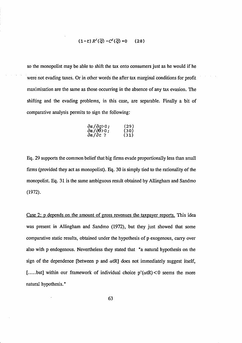
( l - t ) i ? / ( g ) - C / ( g ) = 0 ( 28 )

so the monopolist may be able to shift the tax onto consumers just as he would if he

were not evading taxes. Or in other words the after tax marginal conditions for profit

maximisation are the same as those occurring in the absence of any tax evasion. The

shifting and the evading problems, in this case, are separable. Finally a bit of

comparative analysis permits to sign the following:

d a / d q > 0 ; (2 9 )d a / d Q > 0 ; (3 0 )d a / d t ? (3 1 )

Eq. 29 supports the common belief that big firms evade proportionally less than small

firms (provided they act as monopolist). Eq. 30 is simply tied to the rationality of the

monopolist. Eq. 31 is the same ambiguous result obtained by Allingham and Sandmo

(1972).

Case 2: p depends on the amount of gross revenues the taxpayer reports. This idea

was present in Allingham and Sandmo (1972), but they just showed that some

comparative static results, obtained under the hypothesis of p exogenous, carry over

also with p endogenous. Nevertheless they stated that ”a natural hypothesis on the

sign of the dependence [between p and atR] does not immediately suggest itself,

[ but] within our framework of individual choice p’(atR)<0 seems the more

natural hypothesis.”

63

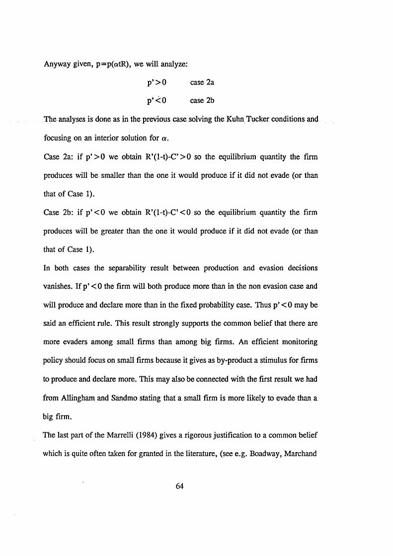
Anyway given, p=p(atR), we will analyze:

p’ > 0 case 2 a

p ’ < 0 case 2 b

The analyses is done as in the previous case solving the Kuhn Tucker conditions and

focusing on an interior solution for a.

Case 2a: if p’> 0 we obtain R’(l-t)-C’ > 0 so the equilibrium quantity the firm

produces will be smaller than the one it would produce if it did not evade (or than

that of Case 1).

Case 2b: if p’< 0 we obtain R*(l-t)-C’< 0 so the equilibrium quantity the firm

produces will be greater than the one it would produce if it did not evade (or than

that of Case 1).

In both cases the separability result between production and evasion decisions

vanishes. If p* < 0 the firm will both produce more than in the non evasion case and

will produce and declare more than in the fixed probability case. Thus p ’ < 0 may be

said an efficient rule. This result strongly supports the common belief that there are

more evaders among small firms than among big firms. An efficient monitoring

policy should focus on small firms because it gives as by-product a stimulus for firms

to produce and declare more. This may also be connected with the first result we had

from Allingham and Sandmo stating that a small firm is more likely to evade than a

big firm.

The last part of the Marrelli (1984) gives a rigorous justification to a common belief

which is quite often taken for granted in the literature, (see e.g. Boadway, Marchand

64

and Pestieau (1992)): direct taxes are more likely to be evaded than indirect taxes.

Actually Marrelli shows that, in presence of absolute decreasing risk aversion, if

direct and indirect taxes yield a priori the same total tax receipts, the optimal interior

rate of indirect tax declaration will be greater than the corresponding direct tax one.

Marrelli (1984) considers a very particular problem (the optimal tax declaration for

a price maker), but it has the merit to have initiated the literature of indirect tax

evasion and to have proved some general results.

3.2 The Social Perspective Approach and Indirect Tax Evasion

Although papers are very rare in this area we are lucky enough to have an article by

Cremer and Gahvari appeared in the February 1993 issue of the Journal of Public

Economics. This is not only one of the most recent papers focusing on this issue, but

also the first (to my knowledge) so complete and self-contained.

The paper considers a competitive economy consisting of n industries producing n

different commodities and a Government levying ad valorem taxes tR. Differently

from other papers evasion is not free, but there is a per unit cost of concealing

resources given by the function 7 =yj(l-a), where 7 ’ > 0 .

The tax administration audits and discovers as cheating a fraction p of firms. The

firms that are caught cheating are taxed on the true amount of their sales and, in

addition, have to pay a fine proportional to the amount of tax evaded. A competitive

firm in the industry i maximises its expected profits:

65

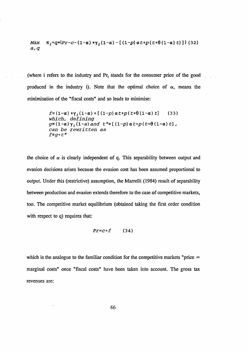
Max 7ii = g * { P r - c - ( 1 - a ) * y± ( 1 - a ) - [ ( 1 - p ) a t + p ( fc+0 ( 1 - a ) t) ]) (32) a , q

(where i refers to the industry and Pq stands for the consumer price of the good

produced in the industry i). Note that the optimal choice of a , means the

minimisation of the "fiscal costs" and so leads to minimise:

f = ( 1 - a ) *yi ( 1 - a ) + [ ( 1 - p ) a t +p( t+0 ( 1 - a ) t ] (33) w h i c h , d e f i n i n gg= ( 1 - a ) y i ( 1 - a ) a n d t e= [ ( 1 - p ) a t+ p ( t+0 ( 1 - a ) t] ,can b e r e w r i t t e n a sf = g + t e

the choice of a is clearly independent of q. This separability between output and

evasion decisions arises because the evasion cost has been assumed proportional to

output. Under this (restrictive) assumption, the Marrelli (1984) result of separability

between production and evasion extends therefore to the case of competitive markets,

too. The competitive market equilibrium (obtained taking the first order condition

with respect to q) requires that:

P r = c + f (34)

which is the analogue to the familiar condition for the competitive markets "price =

marginal costs" once "fiscal costs" have been taken into account. The gross tax

revenues are:

66

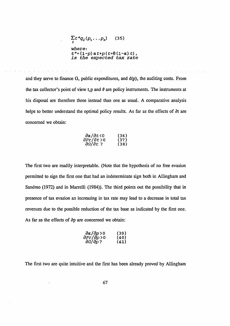
^ t 0q i ( p 1. . . p n) (35)

w h e r e :t e= (1 -p ) a t + p ( t+0 (1 - a ) t ) , i s t h e e x p e c t e d t a x r a t e

and they serve to finance G, public expenditures, and d(p), the auditing costs. From

the tax collector’s point of view t,p and 0 are policy instruments. The instruments at

his disposal are therefore three instead than one as usual. A comparative analysis

helps to better understand the optimal policy results. As far as the effects of dt are

concerned we obtain:

d a / d t < 0 (36)d P r / d t >0 (37)d G / d t ? (38)

The first two are readily interpretable. (Note that the hypothesis of no free evasion

permitted to sign the first one that had an indeterminate sign both in Allingham and

Sandmo (1972) and in Marrelli (1984)). The third points out the possibility that in

presence of tax evasion an increasing in tax rate may lead to a decrease in total tax

revenues due to the possible reduction of the tax base as indicated by the first one.

As far as the effects of dp are concerned we obtain:

d a / d p > 0 (39)d P r / d p >0 (40)d G / d p ? (41)

The first two are quite intuitive and the first has been already proved by Allingham

67

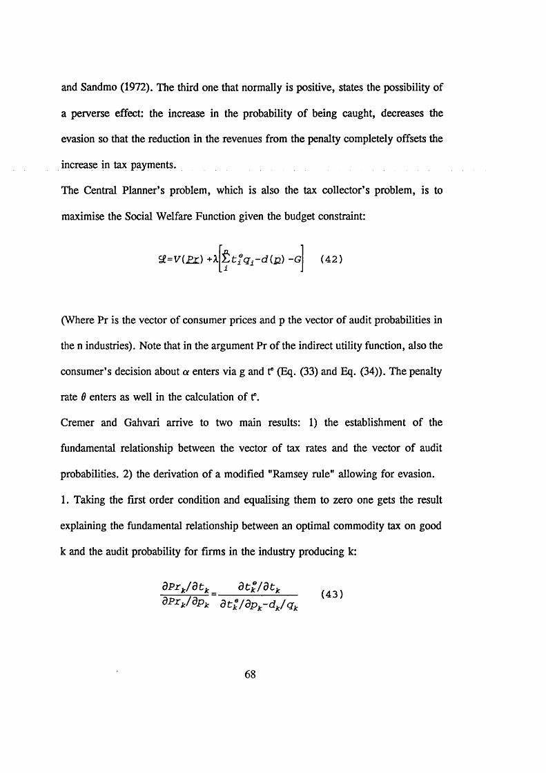
and Sandmo (1972). The third one that normally is positive, states the possibility of

a perverse effect: the increase in the probability of being caught, decreases the

evasion so that the reduction in the revenues from the penalty completely offsets the

increase in tax payments.

The Central Planner’s problem, which is also the tax collector’s problem, is to

maximise the Social Welfare Function given the budget constraint:

S £ = V ( P r ) +X t , t f q i - d { u ) ~G ( 4 2 )

(Where Pr is the vector of consumer prices and p the vector of audit probabilities in

the n industries). Note that in the argument Pr of the indirect utility function, also the

consumer’s decision about a enters via g and te (Eq. (33) and Eq. (34)). The penalty

rate 6 enters as well in the calculation of f .

Cremer and Gahvari arrive to two main results: 1) the establishment of the

fundamental relationship between the vector of tax rates and the vector of audit

probabilities. 2) the derivation of a modified "Ramsey rule" allowing for evasion.

1. Taking the first order condition and equalising them to zero one gets the result

explaining the fundamental relationship between an optimal commodity tax on good

k and the audit probability for firms in the industry producing k:

d P i J d t k _ d t £ / d t k (4;j)dPrk/ d p k d t Z / d p k- d k/ q k

68

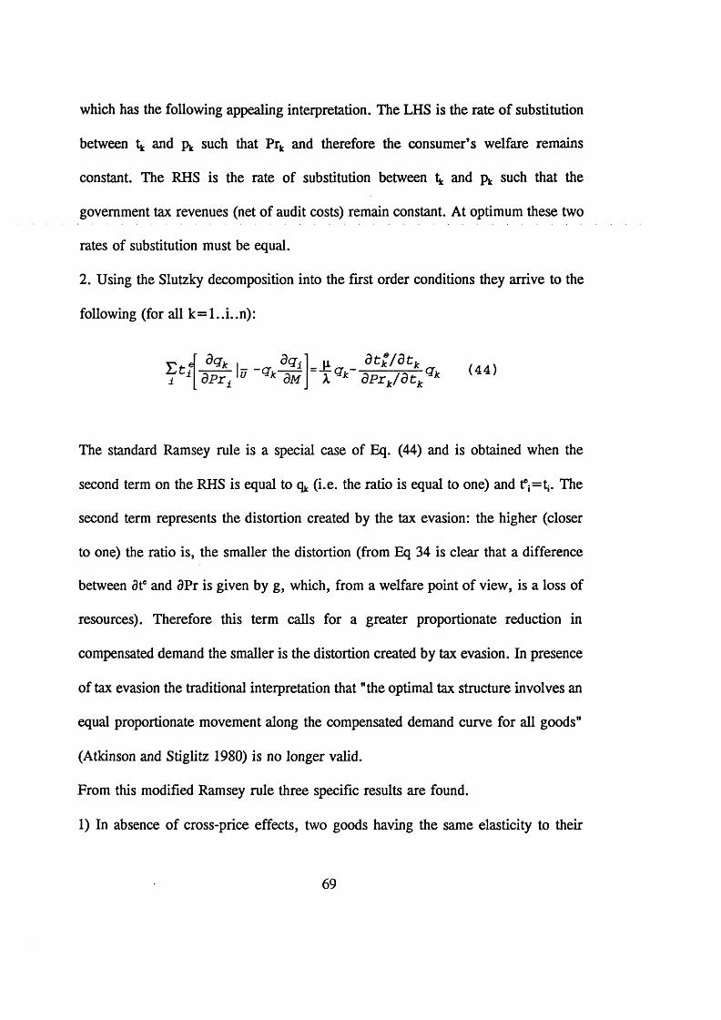
which has the following appealing interpretation. The LHS is the rate of substitution

between t*. and p* such that Prk and therefore the consumer’s welfare remains

constant. The RHS is the rate of substitution between ^ and pk such that the

government tax revenues (net of audit costs) remain constant. At optimum these two

rates of substitution must be equal.

2. Using the Slutzky decomposition into the first order conditions they arrive to the

following (for all k= l..i..n ):

E t i d <3k I _ _0P r, lc/ dM

n 0 tj= d P r J d t t Qk (

The standard Ramsey rule is a special case of Eq. (44) and is obtained when the

second term on the RHS is equal to q . (i.e. the ratio is equal to one) and tei= ti. The

second term represents the distortion created by the tax evasion: the higher (closer

to one) the ratio is, the smaller the distortion (from Eq 34 is clear that a difference

between 3te and 3Pr is given by g, which, from a welfare point of view, is a loss of

resources). Therefore this term calls for a greater proportionate reduction in

compensated demand the smaller is the distortion created by tax evasion. In presence

of tax evasion the traditional interpretation that "the optimal tax structure involves an

equal proportionate movement along the compensated demand curve for all goods"

(Atkinson and Stiglitz 1980) is no longer valid.

From this modified Ramsey rule three specific results are found.

1) In absence of cross-price effects, two goods having the same elasticity to their

69

prices need to be taxed differently if the evasion in the two markets is different.

Namely the expected tax rate in the market subject to more tax evasion will be less

than in the market with less tax evasion. But the optimal legislated tax rate (assuming

equal costs and prices in both markets) will be higher on the good where tax evasion

is higher.

2) In presence of tax evasion, exogenous income does not imply that uniform taxation

of all goods is optimal. This result has a clear interpretation: if tax evasion is an

option "reported" income is no longer exogenous even if the income itself is

exogenous.

3) Wage and uniform commodity taxation are no longer equivalent (somewhat

obvious given the second result).

4. Concluding Remarks

The aim of this survey was to assess the state of the art in the indirect tax evasion

literature, which consists of ten papers at most, and to compare it to the direct tax

evasion literature which counts a few hundred papers and books. We showed that the

two main approaches adopted in the direct tax evasion literature are adopted in the

indirect tax evasion literature as well. We think that the development and the present

state of the art of both literatures is so similar that they share the same strengths and

the same weaknesses. Four main points are worth to be underlined:

1) Both literatures arrive at an optimal taxation result when the case of tax evasion

is taken into account. Both literatures arrive also at the result, quite intuitive, that

70

those who declare less are more likely to have evaded a larger amount of taxes than

those who declare more. Could be interesting to refine this result assuming many

types of individuals under Government imperfect information.

2) Evasion is better fought using all three instruments: t, p, 6. There is a trade off

between p and 9 and it is possible to determine a kind of marginal rule for p and t.

Generally speaking, if evasion is not so widespread p and 6 are enough: when evasion

becomes a mass phenomenon a suitable t has to be chosen, too. However there does

not seem to be evidence that evasion should necessarily call for lower tax rates.

3) Both literatures are quite unknown. Nevertheless evasion is a present problem and

"for the immediate future, at least, [...] is here to stay” (Cowell 1990): we do think

that the results already obtained should be better known and more efforts should be

invested in discovering new ones.

4) Many and deeper thoughts are necessary about the economic treatment of illegal

activities: we should wonder if efficiency arguments are enough to allow a (partial)

accommodation of illegal activities as tax evasion. If this is case, it means that we are

ready to accept that two agents with similar earned income have different level of

welfare depending on their degree of tax compliance. In presence of tax evasion,

when the competitive equilibrium is reached as a decentralized solution, evaders may

be better off than honest citizens. This seems at odds with the widely accepted notion

of horizontal equity. With the partial exception of Cowell (1990) the literature on tax

evasion has never dealt with this aspect.

71

Legend

E(U)= Expected Utility Function U = Utility Function.W = Actual income.R= Revenues from sale:

=R(q)= in monopolistic case,= p r * q = in perfect competition case, where:Pr=price per unit, q=quantity: number of units.

R’(q)= marginal revenue.C (q)= cost function.C ,( q ) = c = marginal cost.

G= government expenditures.L = labour supply in regular market.E= labour supply in irregular market.X= post tax income (i.e. consumption) in case of non evasion.Y = post tax income (i.e. consumption) in case of evasion and no detection.Z = post tax income (i.e. consumption) in case of evasion and detection.

n= index for non evader taxpayers.e= index for evader taxpayers.a — proportion of declared income on total income.7 = cost function of concealing income. t= marginal tax rate.T = lump sum element of the income tax schedule (subsidy if T > 0 , tax if T <0). te= expected tax rate.6— penalty rate.p= probability of being caught.d(g)= costs of auditing.f= fiscal costsg= costs of evading taxes.So ,= reputation in state 0 , 1 .4>= net social marginal utility of income.

ARAX= absolute risk aversion at income X.

72

References

Allingham, M.G. and A. Sandmo, 1972, Income tax evasion: a theoretical analysis, Journal of Public Economics 1, 323-338.

Arrow, K.J., 1970, Essays in the theory of risk-bearing. North-Holland.

Atkinson, A.B. and J. Stiglitz, 1980, Lectures on public economics, Mc-Graw Hill, New-York and London.

Becker, G.S., 1968, Crime and punishment: an economic approach, Journal of Political Economy 76, 169-217

Boadway R., M. Marchand and P. Pestieau, 1992, Towards a theory of the direct- indirect tax mix, CORE Discussion Paper 9226.

Cowell, F., 1985, The economic analysis of tax evasion: a survey, Bulletin of Economic Research 37, 163-193.

Cowell, F., 1990, Cheating the government: the economics of evasion, M.I.T. Press. Cambridge, Mass.

Cremer, H. and F. Gahvari, 1993, Tax evasion and optimal commodity taxation, Journal of Public Economics 50, 261-275.

Kolm, S.C., 1973, A note on optimum tax evasion, Journal of Public Economics 2, 265-270.

Marrelli, M., 1984, On indirect tax evasion, Journal of Public Economics 25, 181- 196.

Mossin, J., 1968a, Aspects of rational insurance purchasing, Journal of Political Economy 76, 553-568.

Mossin, J., 1968b, Taxation and risk-taking: an expected utility approach, Economica 35, 74-82.

Sandmo, A., 1981, Income tax evasion, labour supply, and the equity efficiency tradeoff, Journal of Public Economics 16, 265-288.

Virmani A., 1989, Indirect tax evasion and production efficiency, Journal of Public Economics 39,223-237.

73

Chapter 3

TAX STRUCTURE, TAX REFORM AND TAX EVASION*

Mario Nava Center fo r Economic Performance

London School o f Economics,

Abstract

In this paper we explore whether the shift from an ad valorem tax to a value added tax (which is a prerequisite to join the European Union) improves the "integrity" (number of people in the regular market) and the "efficiency" (total tax revenues) of the tax system. A model of two parallel (black and regular) markets is analyzed. The production in both the black and the regular market is divided in three stages: raw material, intermediate good and final good. Firstly, we prove that if an ad valorem tax is levied, at all stages of the regular market, any, even partial, tax reform towards VAT unequivocally increases integrity (the number of agents). Secondly, we prove that efficiency of the tax system is a direct function of its integrity. Therefore a tax reform from ad valorem to VAT seems justifiable under these two criteria. As a passing result, regular market consumers* welfare is shown to increase.

* Thanks are due to Kevin Roberts for invaluable assistance and to all participants to the 1994 London Jamboree, of the European Doctoral Program in Quantitative Economics for their comments. Excellent written and oral comments by Mick Keen and Tim Besley have been of great assistance in shaping the final version. The usual disclaimers apply.

74

1. Introduction

The literature on Tax Evasion is 22 years old and contains roughly 210 papers. About 200 of

them focuses on direct tax evasion, the rest on indirect tax evasion1. The approach of the vast

majority of papers may be divided in two broad types: the taxpayer’s point of view and the tax

collector’s point of view. The first approach explores the taxpayer’s choice under the uncertainty

on whether or not to report the complete tax base. Usually the aim is to determine, under

reasonable conditions, the optimal fraction of tax base to report. The second approach examines

the choices of the tax collector who has to set the optimal tax rate knowing that evasion is a

possible option for agents. The best papers following this second approach offer as their main

contribution a modified Mirrlees-Stiglitz result for direct taxation and a modified Ramsey rule

for indirect taxation. The modifications are due to fact that face to tax evasion the State also has

some additional instruments to fight it: usually a penalty rate and a probability to catch evaders.

As mentioned in the previous chapter if detection is costly and penalty is not, for the State the

optimal choice is therefore to "hang the evaders with probability close to zero" and this applies

to risk neutral as well as to risk averse individuals. If anything (e.g. moral considerations)

reduces the maximum penalty to less than "hanging" and political argument forces for a

minimum detection activity, the solution is again likely to be a comer solution with the

maximum possible penalty and the minimum possible detection activity.

As far as the taxpayer’s point of view is concerned, I have borrowed Kolm’s word (1973): "This

is hardly Public Economics; in fact it is very private. What is Public Economics is the tax

1 For a recent survey of tax evasion literature from Allingham and Sandmo (1972) seminal paper, to Cremer and Gahvary (1993), see the previous chapter of this thesis.

75

collectors point of view". Indeed, the taxpayer’s point of view is basically an exercise of

maximization under uncertainty. The tax collector’s point of view, being a derivation of the

Mirrlees approach, is embedded into Public Economics literature and it is regarded as the main

theoretical answer to the tax evasion question.

However, the core characteristic of both approaches is similar: given a certain tax structure they

seek to maximize a Utility Function and a Social Welfare Function, respectively.

Differently from this, the present paper focuses on a comparison between two tax structures: an

"ad valorem tax" and a "value added tax" (respectively AVT and VAT henceforth). The point

we want to address is the following: if economic agents (profit maximizing firms and utility

maximizing consumers) had the choice, subject to certain conditions, between a regular and a

black market, how would their choices be affected by the tax system? In other words, which of

the two tax structure attracts more agents into the regular market? Which effect does this have

on the total tax revenues? Which effect does it have on prices and quantities produced in the

regular market?

For the purpose of this paper we shall define the integrity of a tax system as a direct function

of the number of people in the regular market and the efficiency of the tax system as a direct

function of total tax revenue. We will show how integrity and efficiency are affected by a

change from AVT to VAT.

The motivation for this paper comes from the fact that having a VAT system is a requirement

imposed to candidate members of European Union. In the economic literature and among

practitioners this requirement is justified on the production efficiency ground: VAT is superior

to AVT since it does not interfere with the production decisions and allows inputs to enter the

76

production function free of taxes. In this paper we wish to evaluate, not in terms of production

efficiency, but in terms of integrity and efficiency of the tax system as defined above, the effects

of a shift from AVT to VAT. It will be shown that such a move unequivocally increases

integrity and that efficiency is a direct function of integrity. This provides a justification to this

requirement on a ground quite different from the standard production neutrality one. As a

passing result we will show that the ever-honest consumers* surplus increases.

The plan of the paper is as follows. Section 2 compares the core characteristics of an AVT and

a VAT systems. Section 3 and 4 introduce the model under AVT and VAT, respectively. Section

4.1 and 4.2 analyze the effects in terms of integrity and efficiency of a VAT to the first stage

of production and to all stages of production, respectively and section 4.3 compares the results

of the two previous sections. Section 5 concludes.

2. Model Characteristics: AVT vs VAT.

To address our point about tax evasion, we assume that there are two parallel markets: the

regular one and the black one. The Government is able to levy taxes only in the regular market.

Each firm can choose in which market to operate and does so following a profit maximizing

criterion. In both markets, the good on sale is the same, but in the regular market consumers

are entitled to post-sale assistance while in the black market the seller disappears immediately

after the sale. Therefore prices in the black market are systematically lower than in the regular

market.

The production in both markets is divided in 3 stages: raw material firms, intermediate good

77

firms and final good firms. There is different type of firm for each stage of production. Since

we are not interested in showing how intra-firm decisions are affected by fiscal changes all firms

have the same production function which is a 1 to 1 production function: (i.e. each intermediate

good firm buys one unit of input (raw material) from a raw material firm to produce and sell

one unit of output (intermediate good) to a final good firm which uses it as an input). This

assumption amounts to the imposition of two restrictions to the model. Firstly, there is only one

kind of input: this is a strong assumption and makes analyzing tax effects on input substitution

(e.g. of labour with other factors of production) impossible. Secondly, each firm can only

choose to produce zero or one. The first restriction is so important that it can only be overcome

by writing another paper. We are indeed thinking of this issue as the main extension to this

paper. The second problem can be solved easily in this paper by focusing on the aggregate

market production level instead of the firm production level.

We want to show to what extent the movement of firms from the black to the regular market is

affected by a shift from AVT to VAT.

The VAT model we are thinking of is the one currently used by each country of the European

Union for domestic transaction: the so-called origin system2. The crucial characteristic of a

VAT origin system is that though taxes are neutral with respect to the production Junction,

2 For intra-community trade the system now in place (transitory regime) is an hybrid of origin and destination regime. The Council has urged the Commission to submit a proposition for a definitive regime which should extend the origin system valid for domestic transactions to intra-community ones. At the Verona Ecofin meeting (April 1996) it has been announced that "The Commission will present before the summer its strategic program for a definitive VAT system based in the Member States of origin".

78

goods circulate tax paid. This is made possible by a system of payment and reimbursement (i.e.

a system of credits and debts with the Tax Authorities) which greatly reduces possibilities of

fraud. Each time the good, from raw material to final product, is sold there is a possibility of

control by the Tax Authorities. Goods are sort of earmarked during their evolution "from the

mine to the shop" and it is easy for the Tax Authorities to detect if goods disappear at some

intermediate stage. This means that the VAT system is a sort of "trap": if a good belongs to the

regular market at stage s, it has to belong to the regular market also at stage (s-1) and (s+ 1) and

therefore at all stages from 1 to S, since any intermediate agent would find hard to explain to

the Tax Authorities why having bought a certain quantity of inputs a lower quantity of output

is sold (and/or viceversa). We may therefore claim, without loss of generality, that each firm

has the same type of input and output market.

The AVT model we are thinking of is the most standard one, where a tax t is levied, from the

buyer, at each stage of production. This tax structure, differently from the VAT one, does not

have a built-in possibility of cross-checking. However, in the "real world" when an AVT regime

is in place it may be advantageous to buy in the black market (prices are lower) and to sell in

the regular market (prices are higher), while viceversa is generally unprofitable. In other words

if the inputs are both in the black market, the output might be sold both in the regular and in

the black market; viceversa if the inputs are bought in the regular market the output as well is

likely to be sold in the regular market. This means that under the AVT regime the "trap" effect

only works going downward in the production chain and it is given by profit maximizing

behaviour of the economic agents and not by a built in characteristic of the tax structure. If a

good belongs to the regular market at stage s it will probably belong to the regular market at

79

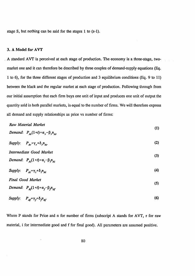
stage S, but nothing can be said for the stages 1 to (s-1).

3. A Model for AVT

A standard AVT is perceived at each stage of production. The economy is a three-stage, two-

market one and it can therefore be described by three couples of demand-supply equations (Eq.

1 to 6 ), for the three different stages of production and 3 equilibrium conditions (Eq. 9 to 11)

between the black and the regular market at each stage of production. Following through from

our initial assumption that each firm buys one unit of input and produces one unit of output the

quantity sold in both parallel markets, is equal to the number of firms. We will therefore express

all demand and supply relationships as price vs number of firms:

Raw Material Market(1)

Demand: >>4r( l +0 =ar~P^i4r

Supply: PAr=tr+S/iAr (2)

Intermediate Good Market(3)

Demand: PAi(l +f)=CL.-$nAi

Supply: PArYj+S,nM (4)

Final Good Market(5)

Demand: PAJ( l +t)=af - pf iAf

Supply: PA/-'<f*^/lAf «*)

Where P stands for Price and n for number of firms (subscript A stands for AVT, r for raw

material, i for intermediate good and f for final good). All parameters are assumed positive.

80

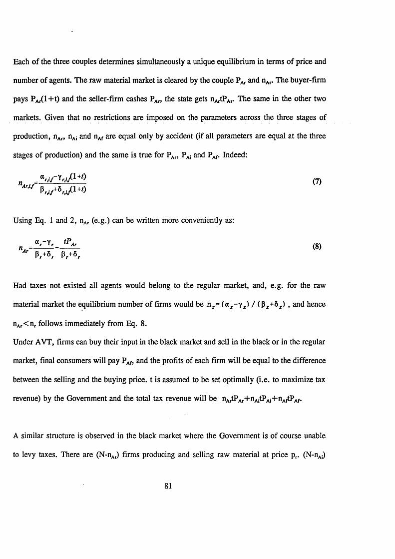
Each of the three couples determines simultaneously a unique equilibrium in terms of price and

number of agents. The raw material market is cleared by the couple PAr and nAr. The buyer-firm

pays PAr(l+ t) and the seller-firm cashes Pad the state gets nArtPAr. The same in the other two

markets. Given that no restrictions are imposed on the parameters across the three stages of

production, nAr, nAi and nAf are equal only by accident (if all parameters are equal at the three

stages of production) and the same is true for Pad PAi and Pat- Indeed:

nArti f

Using Eq. 1 and 2, nAr (e.g.) can be written more conveniently as:

(8)Ar

M 8 , Pr+ 8 r

Had taxes not existed all agents would belong to the regular market, and, e.g. for the raw

material market the equilibrium number of firms would be n T= (aT- y r) / (Pr +5r ) , and hence

nAr< n r follows immediately from Eq. 8 .

Under AVT, firms can buy their input in the black market and sell in the black or in the regular

market, final consumers will pay PAf> and the profits of each firm will be equal to the difference

between the selling and the buying price, t is assumed to be set optimally (i.e. to maximize tax

revenue) by the Government and the total tax revenue will be nArtPAr+nAitPAi+ nAftPAf.

A similar structure is observed in the black market where the Government is of course unable

to levy taxes. There are (N-nAr) firms producing and selling raw material at price pr. (N-nAi)

81

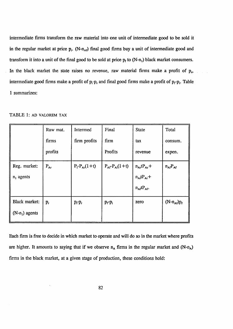
intermediate firms transform the raw material into one unit of intermediate good to be sold it

in the regular market at price p{. (N-nAf) final good firms buy a unit of intermediate good and

transform it into a unit of the final good to be sold at price pf to (N-nj) black market consumers.

In the black market the state raises no revenue, raw material firms make a profit pf pr,

intermediate good firms make a profit of prpr and final good firms make a profit of pr pj. Table

1 summarizes:

TABLE 1: AD VALOREM TAX

Raw mat.

firms

profits

Intermed

firm profits

Final

firm

Profits

State

tax

revenue

Total

consum.

expen.

Reg. market:

nj agents

PAr PrPAr(l+t) PArP Ai(l+ 0 nArtPAr+

nAitPAi+

nAftPAf*

nAfPAf

Black market:

(N-n,) agents

Pr PfPr PrPi zero (N-nAf)pf

Each firm is free to decide in which market to operate and will do so in the market where profits

are higher. It amounts to saying that if we observe nA firms in the regular market and (N-n^

firms in the black market, at a given stage of production, these conditions hold:

82

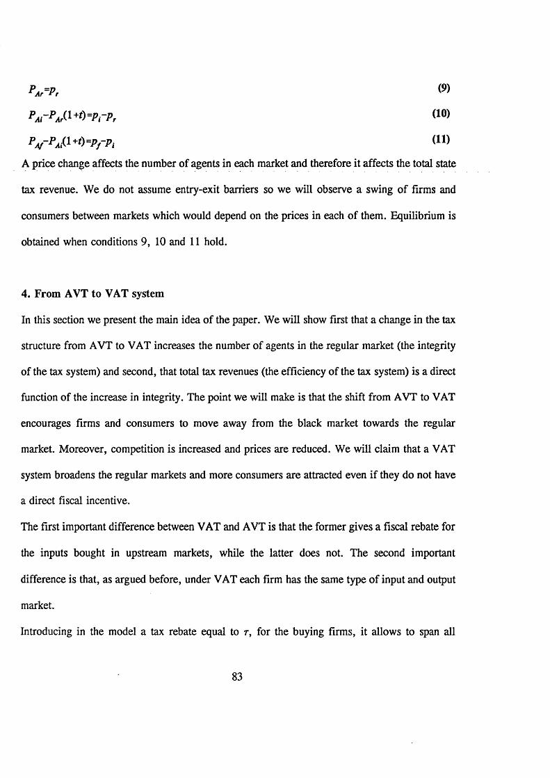
P*rP, »

PA rPAr(-l+t) =PrPr <10>

PA f PA ^ > P f P i (11)

A price change affects the number of agents in each market and therefore it affects the total state

tax revenue. We do not assume entry-exit barriers so we will observe a swing of firms and

consumers between markets which would depend on the prices in each of them. Equilibrium is

obtained when conditions 9, 10 and 11 hold.

4. From AVT to VAT system

In this section we present the main idea of the paper. We will show first that a change in the tax

structure from AVT to VAT increases the number of agents in the regular market (the integrity

of the tax system) and second, that total tax revenues (the efficiency of the tax system) is a direct

function of the increase in integrity. The point we will make is that the shift from AVT to VAT

encourages firms and consumers to move away from the black market towards the regular

market. Moreover, competition is increased and prices are reduced. We will claim that a VAT

system broadens the regular markets and more consumers are attracted even if they do not have

a direct fiscal incentive.

The first important difference between VAT and AVT is that the former gives a fiscal rebate for

the inputs bought in upstream markets, while the latter does not. The second important

difference is that, as argued before, under VAT each firm has the same type of input and output

market.

Introducing in the model a tax rebate equal to r, for the buying firms, it allows to span all

83

combinations from AVT to VAT. When 7=0 in all markets we have an AVT system, when 7 = t

in all markets, but the final one, we end up with a complete VAT system.

4.1 VAT only in the raw Material Market.

To describe the new equilibrium under the VAT scheme we start with the hypothesis that a

subsidy 7 (0<zz t ) is granted only in the raw material market. It amounts to saying that we

have a VAT system in the first market and an AVT in the other markets. We want to find out

the consequences in terms of integrity and efficiency in all markets, of changing the fiscal

system in the most upstream market. In order to respect our assumption of equal number of

firms at each stage of production we define the equilibrium for the raw material market, the

intermediate good market and the final good market in three steps.

I Step: The market equilibrium for the raw material market is described by the following couple:

Demand: PvJ(\+t-T:)=(tr- § rn Vr (12)

Supply: Pvr Y r*t>Pvr (13)

(Where V stands for VAT). Solving this system simultaneously one finds (nVr, PVr) where:

( i4 )

F' Pr+8r( l +i - t ) pr+6,

Notice that nVr will also be the number of firms at the intermediate stage of production (by virtue

of VAT) and in the final market as well (by virtue of AVT as mentioned in the last paragraph

of Section 2). It can therefore be called simply nv.

II Step: The market equilibrium for the intermediate good market is defined as follows. Since

84

nv is given by the equilibrium in the raw material market (as described in the I step) and since

t is assumed equal in all markets, suppliers need to offer at the price Pvi such that the point

(Pvi(l+ t), nv) is on the demand curve of the intermediate market:

Demand: P w(l+t)=a|.-p iwK (15)

The price Pvi is found on the demand curve in order to ensure that all the nv firms which have

bought inputs in the raw material market find a buyer when selling their output in the

intermediate market. On the supply side, since nv is given from step I and PV; is determined

from Eq. (15), in order to satisfy the supply curve equation and to avoid over-determination, we

need to allow for the supply to expand:

Supply: ^

The expansion of the supply is accounted for by the term 6 vi. This means that the endogenous

variables of the intermediate good market are therefore Pvi and 5vi since the number of people

nv is given by the solution of the raw material market. Therefore 5vj depends on PVr and nv

determined in the first market and it changes according to the equilibrium solution in the first

market3.

Notice that 5 would normally be thought of as given by the technology. To obtain market

clearing through it, would mean to assume that technological changes do follow changes in

3 To obtain the exact parametrization of the dependence between <5vi and nv one could rewrite Eq. (16) as follows: h vi= { P vi - y ±) / n v and substitute Pvi using Eq. (15) thus obtaining

6 vi=( / n v which shows the (inverse) relationship between 5vi and nv.

85

prices (provoked by changes in taxation). Conceptually this would seem somewhat odd, thought

not inadmissible.

However, the 5 of our model is not a technological parameter: the equations where it appears,

including those it clears, do not show the total production of a given good, but only the amount

o f production o f a given good which is offered in the regular market (the total production being

the sum of what is sold in the regular and in the black market). For example Eq. 13, 16 and 20

represent the supply of the regular market which is not the total supply, given that, there is a

non-zero supply for the black market (as it is hinted by equations 9 to 11). 5 is therefore a

"strategic" parameter which determines only the division of the total production between black

and regular market and it can thus change when market conditions (e.g. taxation) change in any

of the two markets.

This step by step solution of the model allows the price of the raw material to enter the supply

curve of the intermediate sector (through nv) and accounts for the expansion of the supply via

the increase in the value of 6 . The increased number of agents in the regular market and the

expansion of the supply make Pvi lower than PAi. Indeed subtracting Eq 15 from Eq 3 and

making use of Eq.14, one obtains:

III Step: Given nv, the equilibrium in the final good market is determined in the same way as

(17)

or simply using Eq. 14 rearranged:

(1+tXPAi-p v )=Vi(nrrnA) (18)

86

in the intermediate market. The endogenous variables are still the price and the slope of the

supply function (PVf and 5Vt) given that the number of agents in the system is already

determined. This implies that, given the tax rate t to fully satisfy the demand at the quantity nv:

Demand'. Pvp .H )-a f -P p v (19)

the supply has to expand in order to offer nv at the price Pvf:

Supply: Pvf=yf +bvjnv

Being nv> nA in any market and Pvi,f< P Ai, f in the intermediate and in the final market we have

by necessity 5vi<5Ai and dvf<dAf (i.e. the supply expands for positive values of r).

This closes the system of 6 equations (Eq. (12) and (13; Eq. (15) and (16); Eq. (19) and (20))

in 6 unknowns (PVr, nVr; Pvi, 8wi; Pvf, 6 vf) which describes the equilibrium in the regular market

under VAT. Annex 1 gives a textual and diagrammatical explanation of the three steps.

Two conclusions may be drawn from this exercise: the subsidy has a direct effect on the demand

side which provokes an increase in the number of people willing to buy raw material in the

regular market. Since each agent has the same type of market for inputs and outputs, there is

also an increase in the number of agents offering goods in the intermediate good market which

leads to an expansion of the supply (i.e. the supply curve turns clockwise).

The price in the intermediate market is given by Eq. 18 which has a standard interpretation. It

says that the price decrease is equal to the increase in the quantity demanded multiplied by the

elasticity of the demand curve. A similar equation to Eq.18 can be written for the price in the

87

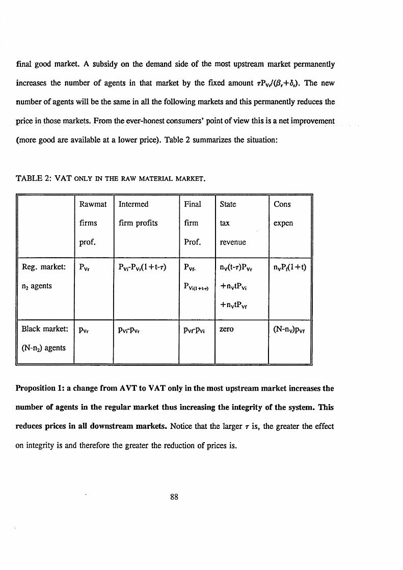
final good market. A subsidy on the demand side of the most upstream market permanently

increases the number of agents in that market by the fixed amount TpyJ((3r+5r). The new

number of agents will be the same in all the following markets and this permanently reduces the

price in those markets. From the ever-honest consumers’ point of view this is a net improvement

(more good are available at a lower price). Table 2 summarizes the situation:

TABLE 2: VAT ONLY IN THE RAW MATERIAL MARKET.

Rawmat

firms

prof.

Intermed

firm profits

Final

firm

Prof.

State

tax

revenue

Cons

expen

Reg. market:

n2 agents

P Vr PyfP vr(H"!_r) Pvr-

P V i(l+t-r)

nv(t-r)PVr

+nvtPvi

+nvtPvf

nvpf(l+t)

Black market:

(N-n2) agents

Pvr PvrPvr PvrPvi zero (N-nv)pvf

Proposition 1: a change from AVT to VAT only in the most upstream market increases the

number of agents in the regular market thus increasing the integrity of the system. This

reduces prices in all downstream markets. Notice that the larger r is, the greater the effect

on integrity is and therefore the greater the reduction of prices is.

88

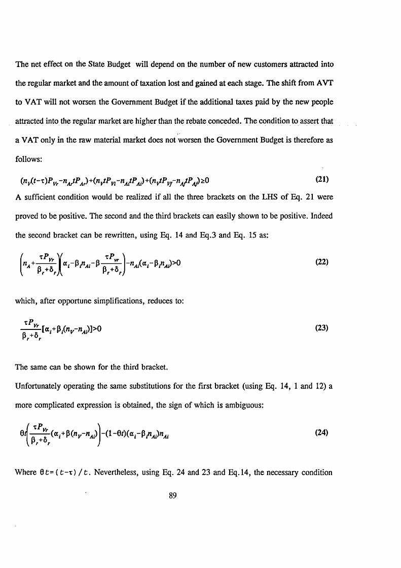
The net effect on the State Budget will depend on the number of new customers attracted into

the regular market and the amount of taxation lost and gained at each stage. The shift from AVT

to VAT will not worsen the Government Budget if the additional taxes paid by the new people

attracted into the regular market are higher than the rebate conceded. The condition to assert that

a VAT only in the raw material market does not worsen the Government Budget is therefore as

follows:

A sufficient condition would be realized if all the three brackets on the LHS of Eq. 21 were

The same can be shown for the third bracket.

Unfortunately operating the same substitutions for the first bracket (using Eq. 14, 1 and 12) a

more complicated expression is obtained, the sign of which is ambiguous:

Where 0 t= ( t - x ) / 1 . Nevertheless, using Eq. 24 and 23 and Eq.14, the necessary condition

(rty(t x)PVr n^tPJ+iriytPyi nA ^ A )+ nv(^vf a) ^ (21)

proved to be positive. The second and the third brackets can easily shown to be positive. Indeed

the second bracket can be rewritten, using Eq. 14 and Eq.3 and Eq. 15 as:

(22)

which, after opportune simplifications, reduces to:

(23)

(24)

89

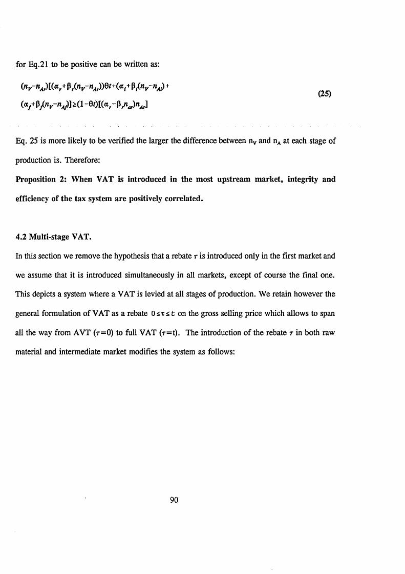
for Eq.21 to be positive can be written as:

(nK-ni4P[(or+Pr(nK-nA))e/+(«,+P,.(«K-nj4(25)

Eq. 25 is more likely to be verified the larger the difference between nv and nA at each stage of

production is. Therefore:

Proposition 2: When VAT is introduced in the most upstream market, integrity and

efficiency of the tax system are positively correlated.

4.2 Multi-stage VAT.

In this section we remove the hypothesis that a rebate r is introduced only in the first market and

we assume that it is introduced simultaneously in all markets, except of course the final one.

This depicts a system where a VAT is levied at all stages of production. We retain however the

general formulation of VAT as a rebate t on the gross selling price which allows to span

all the way from AVT (r=0) to full VAT (r=t). The introduction of the rebate r in both raw

material and intermediate market modifies the system as follows:

90

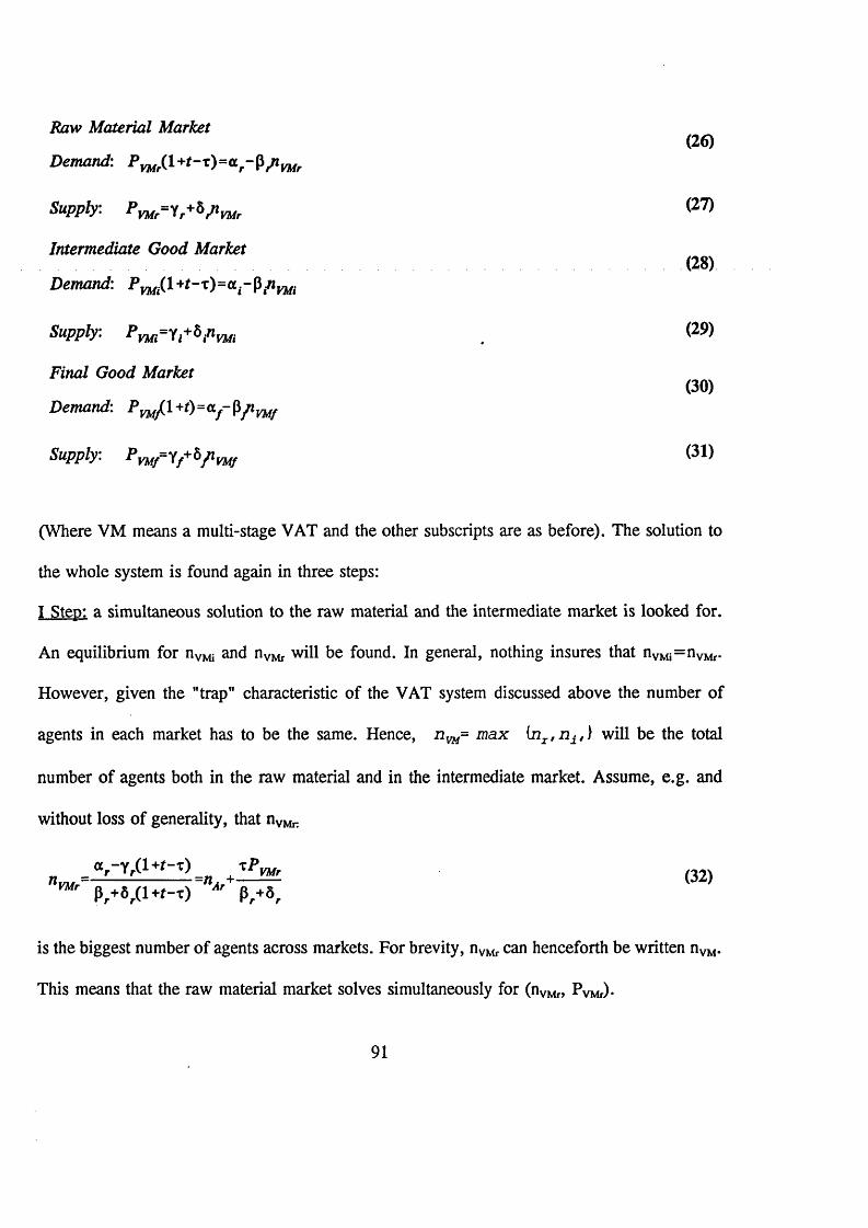
Raw Material Market(26)

Demand:

Supply. Pm = y + l / i mr (27)

Intermediate Good Market(28)

Demand: Pmi( \* t - t> a r ^ f lmi

Supply. P nrrft+ Spnn . <2J>)

Final Good Market(30)

Demand: PmP -+t)=a.f - $ p m f

Supply: P y u n ^ P m t (31)

(Where VM means a multi-stage VAT and the other subscripts are as before). The solution to

the whole system is found again in three steps:

I Step: a simultaneous solution to the raw material and the intermediate market is looked for.

An equilibrium for nVMi and nVMr will be found. In general, nothing insures that nVMi=nVMr.

However, given the "trap” characteristic of the VAT system discussed above the number of

agents in each market has to be the same. Hence, n w= max {nI , n i , ) will be the total

number of agents both in the raw material and in the intermediate market. Assume, e.g. and

without loss of generality, that nVMn

(1+ ,_ T) ^

™' p,+8r(l+f-t) » P,+8,

is the biggest number of agents across markets. For brevity, nVMr can henceforth be written nVM-

This means that the raw material market solves simultaneously for (nVMr, PVMr)-

91

II step and III step: the equilibrium in the other markets is found as in section 4.1. The number

of agents is now given in all markets and is equal to nVM (by virtue of the VAT system), the

price is read on the demand curve of each market, the tax is given at the rate (t-r) in the

intermediate market and t in the final market and the system is solved allowing the supply to

expand in both markets. Effects on prices are identical to section 4.1 and are regulated by the

equivalent of Eq. 18:

03)

Proposition 3: For a given VAT rate, a VAT tax in all markets, but the last one, has

integrity effect greater than or equal to a VAT only in the first market. This implies that

also price reductions are greater than or equal to the case of VAT only in the first market.

Notice that the larger r is, the greater the effect on integrity is and therefore the greater the

reduction of prices is.

To check whether integrity and efficiency are still positively correlated we need to perform an

analysis similar to section 4.1, since the net effect on the State Budget will again depend on the

number of new customers attracted into the regular market and the amount of taxation lost and

gained at each stage. Therefore the conditions to assert that the shift from AVT to VAT at all

stages of production does not worsen the Government Budget is the following:

( j1 v i / t ~ T V M r ~nA r^A r) + (n V fJ t ~ X^ V M i ~ nA ^ A ^ + ( n VMf~n Af>

The sufficient condition would be realized if all the three brackets on the LHS of Eq. 34 were

92

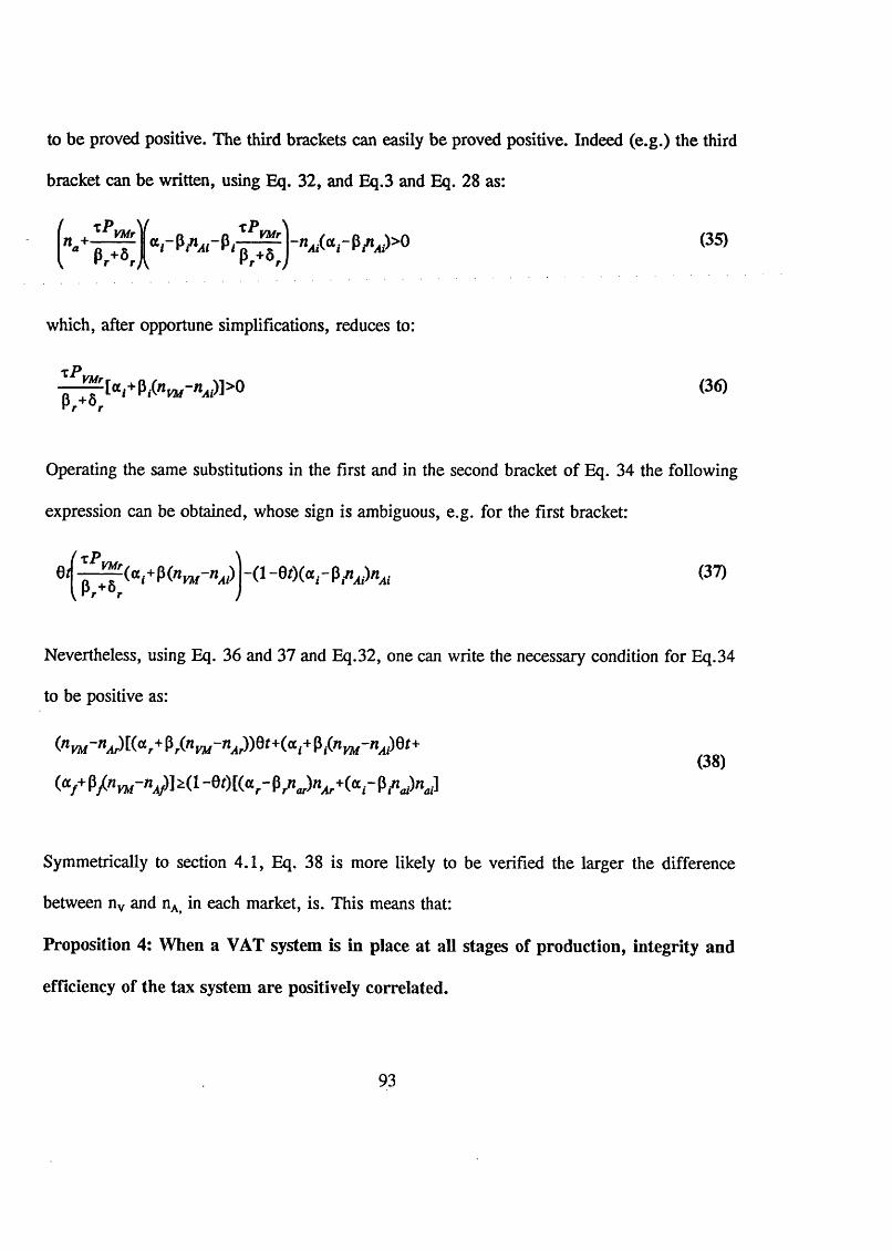
to be proved positive. The third brackets can easily be proved positive. Indeed (e.g.) the third

bracket can be written, using Eq. 32, and Eq.3 and Eq. 28 as:

r P \ / VMr

6 +6 Hr r jai $inAi Pi

T PVMr

6 +6 Hr i- n J a r PpJ> 0 (35)

which, after opportune simplifications, reduces to:

T P VMr

P,+«,(36)

Operating the same substitutions in the first and in the second bracket of Eq. 34 the following

expression can be obtained, whose sign is ambiguous, e.g. for the first bracket:

VMr

6 + 6 \ r r( « , + P - ( 1 - 0 O(ocr P ,^ X i (37)

Nevertheless, using Eq. 36 and 37 and Eq.32, one can write the necessary condition for Eq.34

to be positive as:

(”>«-”J K a r+P /nW -nJ ) e»+(“ i+Pi(nPM'nJ 0' +

(VP/n™~V]a(1'0MK-PA>^+(arP,"<>J(38)

Symmetrically to section 4.1, Eq. 38 is more likely to be verified the larger the difference

between nv and nA> in each market, is. This means that:

Proposition 4: When a VAT system is in place at all stages of production, integrity and

efficiency of the tax system are positively correlated.

93

4.3 Multi stage vs mono-stage VAT

There are two great differences between a system where a tax rebate r is given only in one stage

of production (say stage s) and another where it is given in all stages of production (assume

there are S stages).

First, in the former case, the VAT system chains only three stages of production (s-1, s, s+1),

while in the latter case it chains all stages of production (from 1 to S). The monitoring

possibilities given to the Tax Authorities are much greater under the VAT system and this

reduces the likelihood of fraud.

Second, and related to the first, the implication in terms of integrity. When a tax rebate r is

given only in one stage of production (say stage s) the number of firms will be iv only from

stage s-1 up to the last stage S, but nothing allows to assume it will be so between stage 1 and

stage s-2, given that stages s-2 and s-1 are chained by the AVT system which allows different

numbers of agents at different stages (see last paragraph of section 2). When a VAT system is

extended to all stages of production, nv will be the number of agents in all markets and it will

be equal to: n v= max {n1. . n g. . n j .

Both observations indicate that for a given tax rate the larger is the extent to which VAT is

introduced, the larger is the effect on the integrity of the tax system. We also know from

sections 4.1 and 4.2 that for a given tax structure (multi-stage or mono-stage VAT) the larger

is r, the larger are the effects on integrity and on price reduction.

94

5. Conclusions

Three contributions seem to appear from this paper.

1) Any movement from an ad valorem tax system, to a value added tax system increases the

integrity of the tax system (i.e. the number of agents in the regular market). This is true if the

value added tax is introduced only to some stages of production or to all stages of production.

However, the increase in the number of agents is positively correlated with the extent to which

VAT is introduced.

2) The increase in the efficiency of the tax system depends in turn on the increase in its

integrity. The more additional people enter the regular market the higher tax revenues are.

3) The increased number of agents in the regular market causes a reduction in prices and an

increase in quantities and thus boosts ever-honest consumers’ welfare.

The three above mentioned points answer to our initial question (which are the implications in

terms of integrity and efficiency of the tax system of a shift from ad valorem tax to value added

tax) and therefore justify the European Union requirement for VAT both on the ground of

integrity and efficiency of the tax system and of consumers’ welfare. The first two criteria, as

reasons for having a VAT, have been generally less quoted and less investigated than consumers’

welfare and production neutrality.

We believe that the main merit of this paper is having posed a new question and having

attempted an answer through a very simple model. Nevertheless we are aware that our results

have been derived under restrictive assumptions. Relaxing the strong assumption on the firms’

95

production function (one unit of input is used by each firm to produce one unit of output) might

allow to explain firms* choices of inputs and at firms’ choice of optimal production quantity. In

the framework of our model, it is impossible to ascertain whether a VAT system encourages the

substitution of labour input (which does not enjoy any subsidy) with capital input (which enjoys

a subsidy) or more generally which are the distribution effects of reform towards a VAT system.

This issue shall be the next step in our research.

96

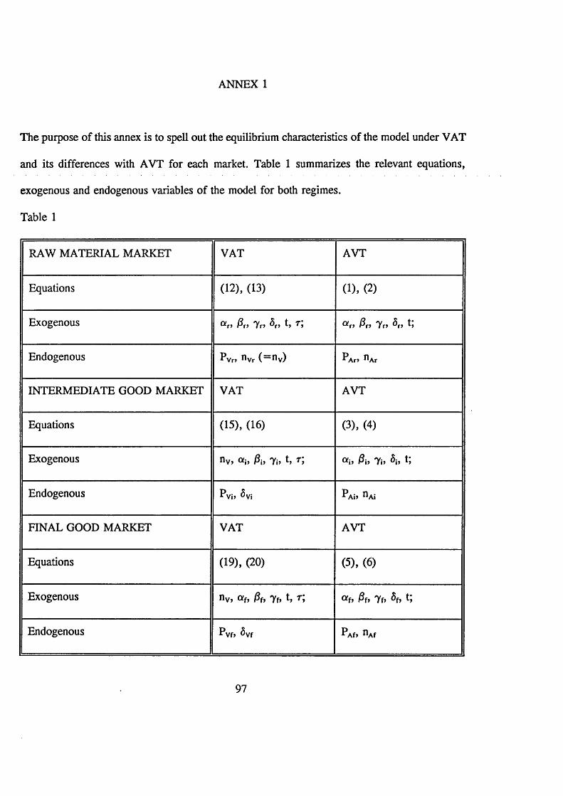
ANNEX 1

The purpose of this annex is to spell out the equilibrium characteristics of the model under VAT

and its differences with AVT for each market. Table 1 summarizes the relevant equations,

exogenous and endogenous variables of the model for both regimes.

Table 1

RAW MATERIAL MARKET VAT AVT

Equations (12), (13) (1), (2)

Exogenous &r> fin Yr> r> L ®n fin Tr» ^n L

Endogenous Pvr> nVr ( = nV) ?Ar» ^Ar

INTERMEDIATE GOOD MARKET VAT AVT

Equations (15), (16) (3), (4)

Exogenous V> ®i> fiii "Yii i> fin Ti> i> L

Endogenous PVj, 5vi Ai> Ai

FINAL GOOD MARKET VAT AVT

Equations (19), (20) (5), (6)

Exogenous nv, fiff af> fiff 7f> f>

Endogenous < o* < Af? nAf

97

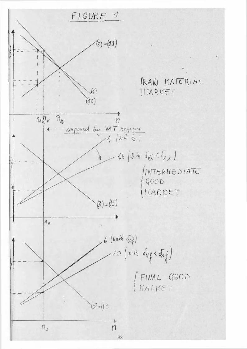
F I 3 U B E 1

i U.v4i

/ K 4 )

PxAvO (1ATC RiAc PfARfCfcT

46 j'JJ-% (4/

f/M I6RH6 b/AJAT

j r t A A / c e r

2 0 ( w J 4

L b

{ t l A R K t T

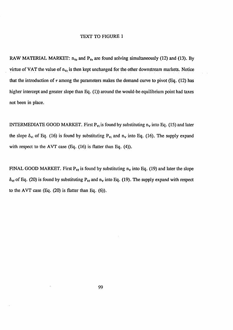
TEXT TO FIGURE 1

RAW MATERIAL MARKET: nVr and PVr are found solving simultaneously (12) and (13). By

virtue of VAT the value of nVr is then kept unchanged for the other downstream markets. Notice

that the introduction of r among the parameters makes the demand curve to pivot (Eq. (12) has

higher intercept and greater slope than Eq. (1)) around the would-be equilibrium point had taxes

not been in place.

INTERMEDIATE GOOD MARKET. First Pvi is found by substituting nv into Eq. (15) and later

the slope 5vi of Eq. (16) is found by substituting Pvi and nv into Eq. (16). The supply expand

with respect to the AVT case (Eq. (16) is flatter than Eq. (4)).

FINAL GOOD MARKET. First Pvf is found by substituting nv into Eq. (19) and later the slope

5vf of Eq. (20) is found by substituting Pvf and nv into Eq. (19). The supply expand with respect

to the AVT case (Eq. (20) is flatter than Eq. (6)).

99

References

Allingham, M.G. and A. Sandmo, 1972, Income tax evasion: a theoretical analysis, Journal of Public Economics 1, 323-338.

Atkinson, A.B. and J. Stiglitz, 1980, Lectures on public economics, Mc-Graw Hill, New-York and London.

Becker, G.S., 1968, Crime and punishment: an economic approach, Journal of Political Economy 76, 169-217

Boadway R., M. Marchand and P. Pestieau, 1992, Towards a theory of the direct-indirect tax mix, CORE Discussion Paper 9226.

Cowell, F., 1985, The economic analysis of tax evasion: a survey, Bulletin of Economic Research 37, 163-193.

Cowell, F., 1990, Cheating the government: the economics of evasion, M.I.T. Press, Cambridge, Mass.

Cowell, F. and J. Gordon, 1993, Auditing with ghosts, Paper prepared for CEPR conference on Organised Crime, Bologna.

Cremer, H. and F. Gahvari, 1993, Tax evasion and optimal commodity taxation, Journal of Public Economics, 50, 261-275.

Kolm, S.C., 1973, A note on optimum tax evasion, Journal of Public Economics 2, 265-270.

Marrelli, M., 1984, On indirect tax evasion, Journal of Public Economics 25, 181-196.

Mirrlees, J.A., 1971, An exploration in the theory of optimum income taxation, Review of Economic Studies 38, 175-208.

Mossin, J., 1968, Taxation and risk-taking: an expected utility approach, Economica 35, 74-82.

Nava, M., M. Marchand and F. Schroyen, 1993, Optimal taxation and provision of public goods with non linear income and linear commodity taxes in a two class economy, CORE Discussion Paper 9321.

Nava, M., F. Schroyen and M. Marchand, 1996, Optimal fiscal and public expenditure policy in a two class economy, Chp.l of this Ph.D. thesis, forthcoming on the Journal of Public Economics, 1996.

100

Sandmo, A., 1981, Income tax evasion, labour supply, and the equity efficiency tradeoff, Journal of Public Economics 16, 265-288.

Varian, H., 1992, Microeconomics Analysis, 3rd ed., W.W. Norton & Company, Inc., New York and London.

Virmani A., 1989, Indirect tax evasion and production efficiency, Journal of Public Economics 39, 223-237.

101

Chapter 4

A NOTE ON CORRUPTION, PRODUCTION AND SHORTAGEIN USSR AND RUSSIA

Mario Nava}Centre fo r Economic Performance,

London School o f Economics

Abstract

Shleifer and Vishny, 1992 argue that privatization increases production and reduces shortage; Komai, 1979 argues that privatization reduces both production and shortage. The transition from USSR to Russia reduced both production and shortage. We argue that this is just the result of the shrinking of the loss-making sector (industrial sector) and the expansion of the profit-making sector (the service sector and namely trade and retailing). We also argue that the validity of Komai’s model is limited to those firms which are overproducing (i.e. more than the profit maximization quantity) and the validity of Shleifer and Vishny’s model is limited to those firms which are underproducing. This reconciles two otherwise contradictory papers.

Keywords: corruption, privatization, shortage, transition.

1 My supervisor Kevin Roberts deserves the greatest thanks. Particular thanks are also due to Richard Layard who initiated me to Russia and to the Russian economy. This chapter has largely benefitted from close contacts with the teachers, namely Amos Witztum and John Board, and the 240 students of the 1993 and 1994 LSE Summer Schools in St.Petersburg and Moscow. Their continuous support and intellectual challenge has been invaluable. The usual disclaimers apply.

102

1. Introduction

"The single most pervasive phenomenon in socialist countries is shortage2 of goods"

(Shleifer and Vishny, 1992). This note aims to reconcile two well-known and prima

facie mutually contradictory papers (Shleifer and Vishny, 1992 and Komai, 1979)

both explaining the causes of shortage in USSR and possible reform programs.

Shleifer and Vishny, 1992 explain shortage with underproduction which is due to

centralized corruption. Komai explains shortage of consumer goods with overuse of

goods as inputs to the industrial sectors. First, we will argue that, in Shleifer and

Vishny’s model, "shortage" is actually a misnomer for "underproduction". Second,

the apparent contradiction between the two models is given by the fact that Shleifer

and Vishny’s model describes only those firms which are producing less than their

profit maximizing quantity, while Komai’s model refers only to those firms which

are producing more than their profit maximizing quantity. The two models therefore

apply on two mutually exclusive subsets of firms.

The empirical evidence which at a first glance seems in favour of Komai (Russia has

less total production and less shortage of goods than the USSR used to have) is

indeed a confirmation of both models: production of goods has declined because of

Komai’s effect and production of services (trade and retailing) has increased because

2 Both economists and non economists agree that looking at shortage is an useful way to look at Capitalism and Socialism. Following Komai (1979) and Weitzman (1984), excess supply of goods distinguish Capitalism while excess demand of goods distinguish Socialism. In the words of common people "In Luga region, cotton stockings are sold only for deceased, on presentation of death certificates by relatives and socks only to war invalids and afghan war veterans. And what should we, the living, wear?" (P.Slepets, Letters to Gorbachev, 1991, pg 28).

103

of the Shleifer and Vishny’s effect thus reducing shortage.

The structure of this note is as follows: section 2 gives a partial description of the

corruption in USSR and discusses the relationship between corruption and shortage

through Shleifer and Vishny’s paper. Section 3 deals with the relationship between

production and shortage and introduces Komai’s article. Section 4 illustrates the

relationship between privatization, production and shortage and tries to reconcile the

findings of both papers. Section 5 concludes.

2. Corruption and Shortage

There is a lot of anecdotal and real evidence about centralized corruption in USSR.

Some excerpts from Remnick, 1993, help to make the point. "The Communist Party

apparatus was the most gigantic mafia the world has ever known. It guarded its

monopoly on power with a sham consensus and backed it up with the force of the

KGB and the Interior Ministry police, (omissis) The trade mafia, [was] a pyramid of

corruption that began in the Communist Party Central Committee and the top

ministers and went all the way down to butchers, bakers and gravediggers, with

everyone getting a piece". Andrei Fyodorov the man who opened the first cooperative

restaurant in Moscow gives the following striking example of a monolithic mafia

"The restaurant director’s salary is R190 a month, say. You can’t live on that, and

so he is forced to take bribes. But there is a system of bribes in USSR. You cannot

get too greedy. A restaurant director cannot take more than R2000/3000 per month.

If he starts taking more, the system grows worried, and in the next five or six months

104

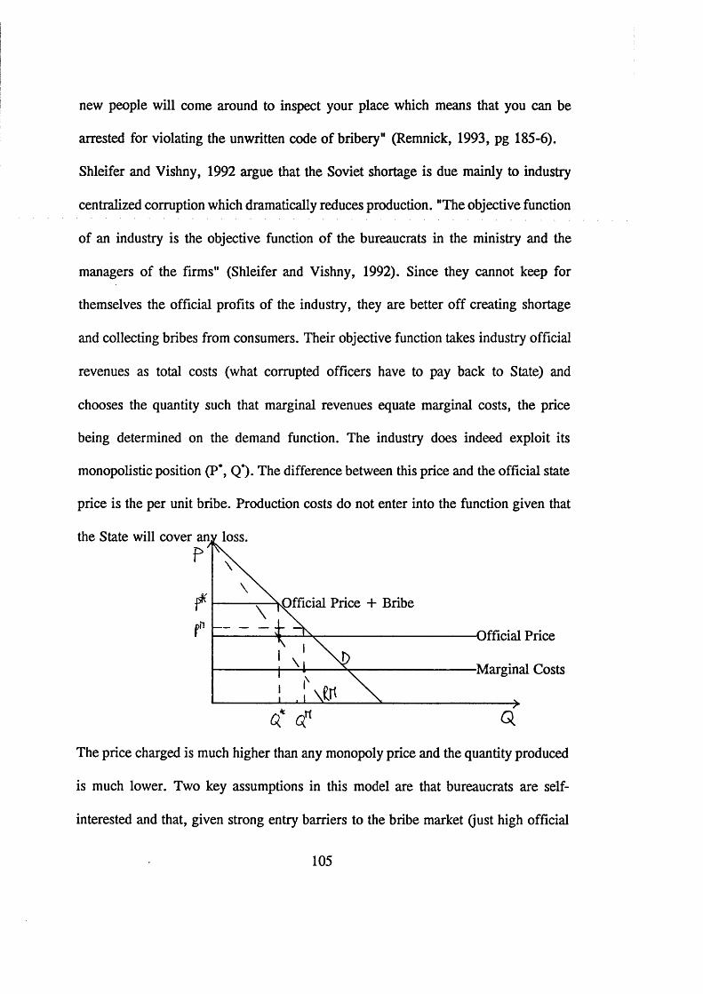
new people will come around to inspect your place which means that you can be

arrested for violating the unwritten code of bribery" (Remnick, 1993, pg 185-6).

Shleifer and Vishny, 1992 argue that the Soviet shortage is due mainly to industry

centralized corruption which dramatically reduces production. "The objective function

of an industry is the objective function of the bureaucrats in the ministry and the

managers of the firms" (Shleifer and Vishny, 1992). Since they cannot keep for

themselves the official profits of the industry, they are better off creating shortage

and collecting bribes from consumers. Their objective function takes industry official

revenues as total costs (what corrupted officers have to pay back to State) and

chooses the quantity such that marginal revenues equate marginal costs, the price

being determined on the demand function. The industry does indeed exploit its

monopolistic position (P*, Q*). The difference between this price and the official state

price is the per unit bribe. Production costs do not enter into the function given that

the State will cover any loss.

Official Price + Bribe

Official Price

■Marginal Costs

The price charged is much higher than any monopoly price and the quantity produced

is much lower. Two key assumptions in this model are that bureaucrats are self-

interested and that, given strong entry barriers to the bribe market (just high official

105

and bureaucrats can ask for them), a cartel of "bribees" is created to maximize total

bribes. The lower the official price is, the more bribes can be extracted. Any attempt

from the State, by increasing official prices (thus increasing firm marginal costs), to

reduce bureaucrats possibility to collect bribes, has the same undesirable result (on

price and quantity) as a per unit tax on a monopoly: it increases prices reducing the

quantity produced. This can be a reason, among others, for the abnormally low prices

in USSR3.

The analysis assumes that firms can choose the quantity to produce. Corruption

reduces the profit maximizing quantity. A possible way out is privatization which

allows the firm to retain profits so production would increase till the monopolistic

level (Pm, Qm) and therefore reduce shortage.

Shleifer and Vishny’s model takes the "centralized corruption" as a fact and builds

on it a possible explanation for shortage based on the fact that corruption reduces

production. Were, for whatever reason, production to increase, shortage would

automatically reduce.

Two key features of the Shleifer and Vishny’s model deserve attention.

First, despite its title, Shleifer and Vishny 1992 throws light on the relationship

*corruption and production" and not "corruption and shortage *. In their article the

concept of "shortage" and the concept of "underproduction" overlap. This approach

3 About possible social considerations leading to lower prices and a quantity rationing see Weitzman (1977).

106

completely disregards distributive trades. In other words they make the implicit

assumption that lack of production is a necessary and sufficient condition for

shortage. Corruption can be taken as a cause of shortage only if both the necessary

and the sufficient condition prove true. Otherwise corruption is only a cause of

underproduction.

The sufficient conditions can be invalidated by imports: this is indeed the case of

small open economies (Luxembourg, Arabian Emirates etc), but hardly the case of

USSR which was basically a closed (within Comecon area) economy. Its share in the

world turnover was one third that of the USA and half that of Japan. Per capita

imports were 1/5 that of the USA and Japan and 1/12 that of Germany. This was

mainly due to the rouble non-convertibility and to high, in real terms, custom

duties4.

The necessary conditions can be invalidated by the existence of obstacles between

production and consumption. In other words even in presence of an high level of

production, goods might not reach consumers due to the imperfection of the

distributive trade. Shortage may appear because there is no production of goods or

because there is no production of the service of distributing goods or both. USSR

statistics (provided one can rely on them) do not show such a significant "lack of

4 "Not long ago I received a present from United States. Its price was about $40 or 1/60 of the average monthly pay of an American worker. I am a worker too. But 1/60 of my pay is R4. Custom duties cost me R160 or 40/60 of my pay. I do not understand why I have to pay customs duties to the State because the State cannot provide me with essential goods. Why?" (V. Bochkarev, Letters to Gorbachev, 1991, pg 63).

107

production" as argued in Shleifer and Vishny. USSR production consisted of many

industries with a high degree of monopolization (some areas were identified by their

only productive activity, for striking example see Remnick, 1993, pg 204-215).

Products were distributed around the Soviet Union by state organizations under

Central Planned orders. A discussion of the ability of the distributive system to

spread goods across the whole Soviet seems a missing piece in Shleifer and Vishny,

1992.

Second, they assume that Soviet firms had some degree of freedom in determining

their output. This might have been true for those firms with "intangible output" like

the firms in the service sector, but surely it was not true for firms in the industrial

sector which had to respect (or at least to produce not less than) a centrally decided

level of output. This second feature restricts the applicability of the Shleifer and

Vishny’s model only to firms in the service sector.

3. Production and Shortage in the USSR.

The official explanation for shortage of goods goes as follows. "The economic

Structure of the Soviet State is based on the socialist system of national economy and

socialist ownership of the instruments and means of production (omissis). A planned

economy rids society of the destructive influence of private competition and anarchy

of production, and rules out economic crises, ensuring continuous growth of

industrial production. The ultimate aim of production is to create an abundance of

material and cultural wealth (omissis). In developing Soviet industry the stress was

108

on the heavy industry (omissis). In order to carry out rapid industrialization the soviet

people made great sacrifices, denying themselves many comforts and even the barest

necessities. Therefore the output o f consumers goods lagged behind producer

goods, (omissis). Heavy industry continues to develop at a somewhat faster rate than

light industry. And this is to be expected since heavy industry forms the basis for the

development of all other branches of national economy, including the consumer goods

industry". (The Soviet Union, Everyman’s Book, 1967, pg 74-78, Italics added).

The Hungarian economist Komai (1979) in a well known article offers an economic

interpretation of the above-mentioned official explanation. Komai attributes the lack

of consumer goods to the unfair competition between consumers and firms.

Consumers face a hard budget constraint while firms face only a soft one. Indeed

being losses automatically compensated by state, the firms’ demand is only limited

by the plan. Firms, the managers of which are interested in producing as much as

possible in order to over-fulfill the plan, may therefore buy everything and leave

consumers "goodless". The common comment about this explanation is that it could

be appropriate for intermediate goods, not for final goods (socks, shoes, cars,

housing). Nevertheless, Komai does stress that lack of production and shortage are

not the same concept. In Komai’s model we have shortage due to overproduction.

This, of course, does not necessarily imply that a reduction in production reduces

shortage. However, it does imply that lack of production is not a necessary condition

for shortage. Indeed, shortage may arise because even if goods are produced they do

109

not reach consumers due to different obstacles5. In Komai’s model firms are

producing a quantity, decided by the Central Planner, much higher than the profit-

maximizing one. Privatization would lead to produce the profit maximizing quantity

and would therefore reduce total production.

4. Privatization, Production and Shortage

As soon as reforms took place and the former Soviet Union became the Russian

Federation a new relationship among shortage, corruption and production developed.

Corruption became much less organized and much more widespread6, shortage

5 Whenever I go to a chemist I am invariably met with the retort "sorry, nocotton wool". Why is this the case when we are the world’s largest producer ofcotton wool? (I. Yelinetsaya, Letters to Gorbachev, 1991, pg 107). In the answer L.Relin, vice chairman of cotton industry, explains that this is due to lack of packing technology and to the huge demand of cottons wool for non-medical purposes. The latter part of the answer seems to confirm Komai’s point.

6 In a second paper, Shleifer and Vishny, 1993, argue also that, if privatization in not carried on, during transition, production falls since there is a change in the structure of corruption. The above mentioned monolithic and monopolistic system of extorting bribes collapsed with the USSR and was replaced by a system where each official acts as an independent monopolist and tries to maximize his or her own revenues. In the Soviet Union all governments goods were allocated by joint monopolist agencies, in Russia by independent monopolistic agencies. In the first case

dx. dx.the optimum is reached where: MRa MR,—J-=MC, V i j and given—->0

Jdx. dx.(governments goods or permits in the same industry are complementary goods) weobtain MR<MC. Vi. In the second case MRi=MCi Vi. Clearly in the second caseproduction is lower, per unit price is higher and the aggregate level of bribes islower. This becomes even worse when there is free entry into collection of bribes.If entry into the collection of bribes were completely free, the per unit bribe wouldrise to infinity while production and bribe revenue fall to zero. As in any othermarket it is therefore in the interest of the incumbent to restrict access.

110

reduced and nearly disappeared and production dramatically collapsed. For corruption

we have to rely on the empirical non-documental evidence, but some shortage and

production data are available7.

Shortage has been reducing steadily since February 1992. The index of availability

of goods (0 means no goods in any city, 100 means all goods in all 132 cities of the

sample) which averaged, on aggregate, 61% during 1992, did rise, on aggregate, to

80% by the end of 1994. It also shows that shortages are more prevalent for

foodstuffs than for non-foodstuffs.

Production, measured by the Gross Domestic Product, fell by 19% in 1992, by 12%

in 1993 and by 15% in 1994. In 1993 and 1994 the production of goods fell by 14%

and 21% respectively, while the production of services fell by only 9% and 10%,

respectively. In the period 1990-1994 the share of goods in the GDP has decreased

from 60,6% to 43,5% while the share of services has increased from 32,4% to

50,0%.

To summarize, Russian production is less than Soviet production, but more goods are

on the shelves of Russian shops than they were on the shelves of Soviet shops, i.e.

shortage is much reduced.

Privatization is the distinctive feature of the Russian transition towards market

system. No other former socialist economy did better than Russia in privatizing

small, medium and large firms. However the privatization process had a different

7 Data from Russian Economic Trends 1995, vol. 4, n.2.

I l l

pace in different sectors. Among small-scale enterprises (retail trade, catering and

services) privatized firms were, by mid 1994, roughly 75% of the market. In some

regions small-scale privatization is almost complete. The process of industrial

privatization took place mainly in 1993 and 1994 and some 75% of the industrial

employment belongs now to privatized enterprises8. To focus on privatization allows

for a solution of the apparent paradox "less shortage and less production".

As argued above, Komai’s model and the Shleifer and Vishny’s model give two

opposite explanations to the shortage problem; however, shortage would disappear

in both models if a widespread privatization program is implemented (as suggested

by Shleifer and Vishny). If privatization continues, losses are not covered, the budget

constraint becomes hard and net profits can be retained.

In Shleifer and Vishny’s model there will be a greater quantity produced at a lower

price so shortage can be eliminated. In Komai’s model, firms will face a hard budget

constraint. Loss-making firms will discontinue production, profit making firms will

produce only till the profit maximizing quantity. The net effect will be negative: in

aggregate, firms will produce fewer goods and therefore will require less inputs so

that more goods will be left to consumers.

The Komai’s model seems to fit the facts accurately. Firms now face a hard budget

constraint, they require less inputs and thus they produce less (total production falls).

Consumers and firms compete fairly to get goods therefore the consumers’ slice is

8 However, "privatization de jure cannot yet be equated with privatization de facto , as many entreprise managers have continued to operate as under state ownership" (RET, Vol.3, N.2).

112

bigger than beforehand (shortage is reduced).

On the other hand, looking at disaggregate data of production, the present situation

can be seen as an evidence in favour of Shleifer and Vishny’s model as well. The

production of those sectors where privatization has been more extensive (service

sector) has fallen much less9 (and in few cases has even risen) than the production

of those sector where privatization is still incomplete (the industrial goods sector). It

is therefore safe to claim that reduction in shortage has been brought about by

privately and domestically produced goods (the Russian trade surplus has been

positive since 1992 though it is believed there is a large amount of unregistered

illegal imports) and increased efficiency of the privatized distributive sector (shops

privatization is basically complete).

5. Conclusions

On one hand, Shleifer and Vishny, 1992 argue that shortage is caused by corruption

(i.e. self-interest bureaucrats collecting bribes from consumers) and privatization (to

allow to appropriate profits) would eliminate shortage. On the other hand, Komai,

1979, argues that shortage is caused by overproduction and unfair competition

between firms (who face a soft budget constraint) and individuals (who face an hard

budget constraint). Firms privatization, during the transition from USSR to Russia,

9 In addition to the data mentioned at the beginning of this section, a striking evidence is given by agriculture. In 1994 the share of households on the total land is no more than 5%, while the share of agricultural state enterprises is about 90%: the former produces 36% of the total gross agricultural output, the latter only 62%!

113

has reduced total production but has also dramatically reduced shortage.

First, we argued that what is referred as shortage in Shleifer and Vishny’s model is

indeed underproduction. Second, we argued that both forecasts were correct since

they applied to two mutually exclusive subsets of firms: Komai’s forecast on

privatization applies to those firms producing more than the profit maximizing

quantity and having a minimum level of production determined by the plan, while

Shleifer and Vishny’ s forecast applies to those producing less than the profit

maximizing quantity and having freedom in choosing their level of production.

Typically, industrial firms belonged to the first subset and were loss-making ones,

while service firms belonged to the second subset and were profit-making ones. This

explain the apparent Russian paradox of "less production and less shortage". It is the

joint result of the Komai’s effect on the industrial sector which has greatly reduced

production (total production has fallen since most previously loss-making firms have

stopped production) and of the Shleifer and Vishny’ effect on the service sector,

namely trade and retailing (profit-making firms have mushroomed in the service

sector) which has greatly reduced shortage.

114

References

Aslund, A. (ed.), 1995, "Russian Economic Reform at Risk", Pinter Publishers, London and New York.

Bhagwati, J.N., 1982, "Directly Unproductive, Profit-Seeking (DUP) Activities", Journal of Political Economy, vol 90, 5, 988-1002.

Harris, J.R. and M.P. Todaro, 1970, "Migration, Unemployment and Development: A Two Sector Analysis", American Economic Review, 60, 126-142.

Komai, J., 1979, "Resource vs Demand-constrained System", Econometrica, vol 47, 4, 801-819.

Krueger, A., 1974, "The political Economy of the Rent seeking Society", American Economic Review, 64, 291-303.

McKay, R. (ed), 1991, "Letters to Gorbachev-Life in Russia Through the Postbag of Argumenty i Fakty", Michael Joseph, London.

Remnick, D., 1993, "Lenin’s Tomb", John Wiley and Son, New York.

Roxborough, W.I. and J. Shapiro, 1994, "Excess Wage Tax", Socio-Economic Survey, Nol7, p.9, Macroeconomics and Finance Unit, Moscow.

Russian Economic Trends (RET), Government of The Russian Federation, Whurr Publishers Ltd, London (1993, 1994 and 1995 issues).

Shleifer, A. and R. Vishny, 1992, "Pervasive Shortage under Socialism", Rand Journal of Economics, XXIII, 237-46.

Shleifer, A. and R. Vishny, 1993, "Corruption", Quarterly Journal of Economics, CVIII, 599-617.

"The Soviet Union Everyman’s Book", Novosti Press Agency Publishing House, Moscow, 1967.

Tullock, G., 1967, "The Welfare Costs of Tariffs, Monopolies and Theft", Western Economic Journal, 5, 224-32.

Weitzman, M.L., 1977, "Is the Price System or Rationing More Effective in Getting a Commodity to Those Who Need it Most", 8 , 517-524.

115

Chapter 5

LABOUR MARKET REALLOCATION AND RENT-SEEKING IN TRANSITION ECONOMY

Mario Nava1 Centre for Economic Performance,

London School o f Economics

Abstract

We present a simple two-sector model of the Russian labour market. Starting from a "full-employment" equilibrium with no search (the USSR), we analyze the path to the new equilibrium with unemployment and search (Russia). The links between the fraction of people searching, the wage differential and the hiring and firing probability of both sectors are investigated. A tentative way to compute these probabilities is proposed starting from recent (91-94) Russian data on unemployment and wages. It is shown that the wage differential across sectors rises with the strengthening of the entry barriers. It is argued that if no action is taken by the Authorities to fight unemployment and to reduce the wage differential across sectors (e.g. relaxing the entry barriers to the most productive sector), the market will react by developing, as an endogenous alternative to unemployment, a third sector which would act as a rent seeking one against the most productive sector. This will increase the outflow of workers from the least productive sector. Finally, it is shown that if the fraction of rent-seeking people attains a critical mass the above-mentioned policies may not be enough to rid the economy of the rent-seeking sector.

Keywords: labour market, rent-seeking, Russia, transition.

1 Special thanks are due to my supervisor, Kevin Roberts, for his dedication to my work, which has contributed to improve dramatically this chapter. A first version of this paper was presented to the 1995 EEA Conference (Prague). I am grateful to all participants, and especially to Josef Konings, for their stimulating comments. Sharp and precise suggestions from Mick Keen have considerably improved the final version. The usual disclaimers apply.

116

1. Introduction

This paper tries to explain labour market adjustments during the transition from

Socialism to Capitalism in Russia. We will propose a model to describe the path from

a full-employment equilibrium with no search and no wage differential across sectors

(the USSR) to an equilibrium with unemployment, with search and wage differential

across sectors (Russia). We will argue that the transition to the market, especially

privatization, the most successful and widespread reform in Russia, provoked a

positive technological shock to the trade sector and a negative one to the industrial

sector. Privatization in the trade sector wiped out shortage and brought goods back

to Russian consumers. Hard budget constraints and incomplete privatization in the

industrial sector reduced production. Labour attracted by the highest expected wage

in the trade sector tries to move away from the lowest productive market and enter

the highest productive market. There are entry barriers to the highest productive

market which prevents wages equalizing thus pushing people into the unemployment

pool. Workers require a minimal wage differential (changing with the fraction of

people searching) to wish to enter the trade sector. This means that, when the wage

differential is very wide, many workers are trying to get into the trade sector and

some of them end up unemployed. The movement of workers from one sector to the

other will bring the economy to a final equilibrium with a lower wage differential

across sectors. We show that an effective Government policy to fight unemployment

would not increase unemployment benefits, but would reduce the wage gap between

markets through complete privatization of the industrial sector and/or the relaxation

117

of the entry barriers to the trade sector. In the absence of intervention we show that

a black sector (where earnings are higher than unemployment benefits) could appear

and tempt those who become unemployed. Finally, it is argued that once the black

sector has appeared and developed, it tends to stay even if the previous obstacles to

completion of the transition towards market economy are removed. This allows for

the second policy conclusion: the timing of the Government intervention matters for

its effectiveness, the earlier the better.

The paper is organized as follows. Section 2 deals with the new Russian labour

market. In section 3 we present a model aimed at describing the labour market

equilibrium. After introducing model assumptions in subsection 3.1, in subsection 3.2

we use a model similar to the well-known Harris Todaro (1970) model to illustrate

the labour market changes due to the transition from the planned economy to the

market economy. In subsection 3.3 we discuss Government policies to fight

unemployment. Recent Russian data to give numerical values to the parameters of the

model are presented in subsection 3.4. In the last two subsections 3.5 and 3.6

possible developments of the equilibrium are discussed when a rent-seeking sector

appears. Section 4 concludes.

2. Labour Market in Russia2.

The labour market changes have been the most dramatic of all. In the USSR, jobs

2 This section draws on "Labour Market Adjustment in Russia" by Richard Layard and Andrea Richter special report on RET, (1994), Vol.3, N.2. A revised version of it is also published in Aslund (1995).

118

were assigned centrally and wages were substantially equal across sectors being

disconnected from the workers’ productivity. In Russia, jobs are now allocated

through a decentralized hiring and firing process and wages are largely different

across sectors. Privatized sectors have higher average productivity than non-privatized

sectors. The society is now divided in classes of different income: those who are

working in a de facto privatized sector and, those who are working in a still non­

privatized sector and the those who are currently unemployed or underemployed.

Unemployment reached 7.7% by June 1995 and underemployment 5.6%. This figures

are very low compared to western ones especially when one relates this to the large

decline in production described chapter 4.

Several explanations have been given for the relatively low rate of unemployment.

Wage flexibility plays an important role in providing job security to workers (in ipid

1994 the minimum wage was roughly 8 % of the average wage). Firms have financial

and strategic reasons not to fire workers: 1) the excess wage tax which entitles firms

to pay less taxes, keeping employees at the minimum wage rather than firing them3.

2) the high severance costs: unemployment benefits for the first 3 months (equal to

100% of the last nominal wage) are paid by employers. 3) access to cheap

government credit may be linked to the number of employees. 4) managers have a

paternalistic attitude towards workers due to long-time acquaintance and many

workers are now shareholders in privatized enterprises.

3 See Roxborough and Shapiro, 1994 or RET, 1994, Vol.3, N.2. For a generalization of both see OECD, 1995)

119

Employees prefer to earn the minimum wage, staying on the books of the firm, than

earning unemployment benefits even if the latter are initially higher because 1)

unemployment benefits are in nominal terms and in the long run they tend to become

negligible; only approximately one third of those who are out of job bother to register

as unemployed. 2 ) dissociating from the firm, workers lose most of the in kind

benefits like free or subsidized meals and food, retraining and education, housing and

health care and the use of enterprise’s tools for some petty second job. Finally 3),

membership of a firm is still a source of social identity. The above-mentioned reasons

may explain why job reallocation has been for Russia a phenomenon more important

than generally in Western Economies.

3. A Model of Labour Market in Transition

In this section we provide a model aiming to explain the present labour market

equilibrium. There are only two sectors in the economy paying two different wage

rates. Workers migrate from one sector to the other maximizing expected utility. This

leads, as in the Harris-Todaro’s model to the existence of an equilibrium with

considerable unemployment, which is bound to create an increasing social discontent.

We will claim that, in the absence of an exogenous intervention eliminating what

causes unemployment and what prevents the equalization of the wage rates, workers

in the unemployment pool, following the expected utility rule, would gather together

and form a third unofficial sector. The third sector, under some mild assumption, will

eventually absorb most of the workers from the least paying sector and will lead to

120

wage rate equalization with even bigger official unemployment and a larger black

economy. It is shown that it would be easier for the Government to act so as to avoid

the development of a black sector than to get rid of it once it has developed.

3.1 Model Assumptions

No doubt the low rate of unemployment in Russia coupled with the collapse of gross

domestic product (GDP) is one of the major economic puzzles to be explained. Our

model tries to describe the movement in the labour market following the transition

from USSR to Russia. We make the following assumption.

1) There are no new entrants in the labour market (we are looking at the short run).

2) There are two sectors: "industrial" and "trade". Their production function are:

L=l(n,,jS) and T=t(nt,a). For both functions the first derivative with respect to n is

positive and the second is negative; n, associated with the respective subscript, stands

for the number of employed in each sector; a and 0 are variables containing

institutional and technological factors.

3) Soviet workers of both sectors used to get a salary disconnected from their

T+Lproductivity: — F° r the Russian economy we assume first that an exogenous

shock has modified the initial values of Wt and W, and later we treat wages

endogenously. The russian wage is a function of the productivity of the sector, the

number of agents in the sector and the entry barriers to the sector:

121

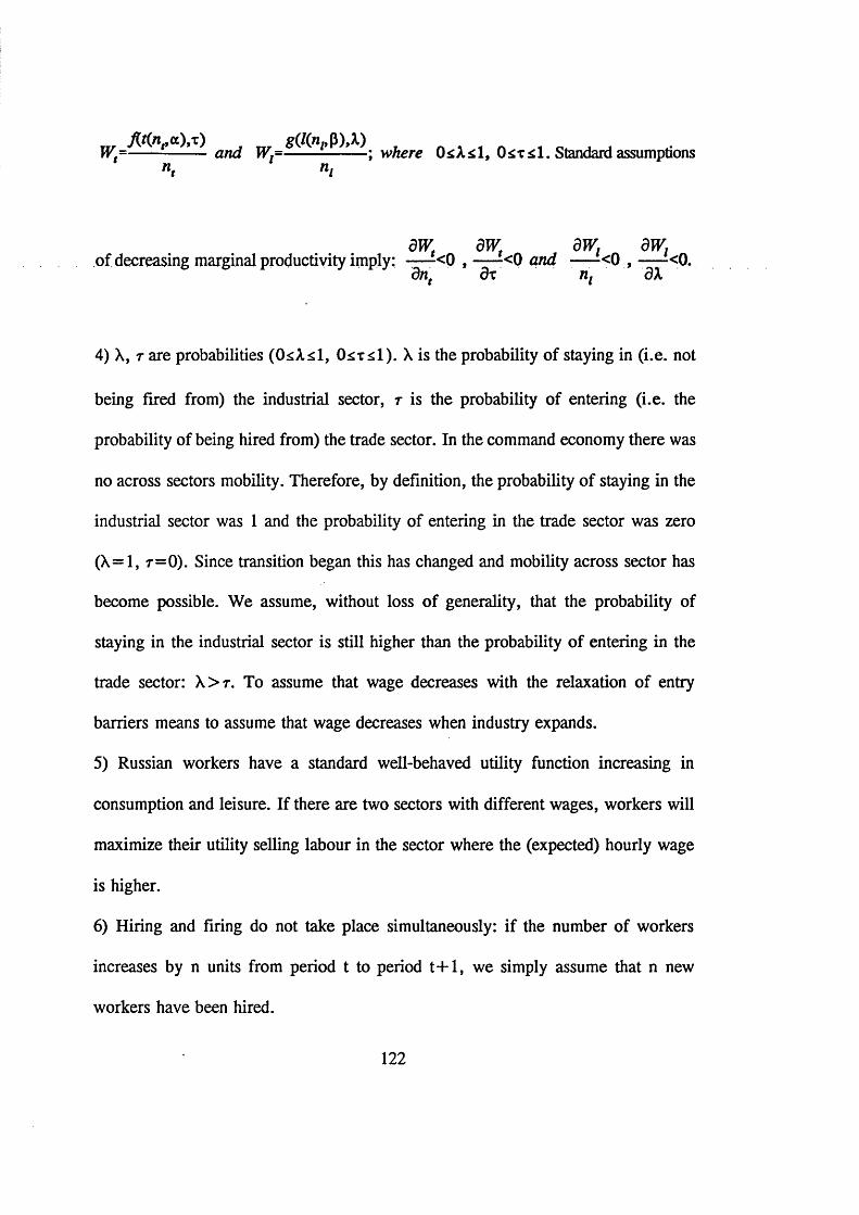
. / W r t - a ) , * ) g (Z (7 i , ,P ) ,A .)W=---------------and W,=------ ; where 0^ Xz 1, Standard assumptions

wr ni

dWt dWt dW, dW.of decreasing marginal productivity imply: -----< 0 , ------ < 0 and -----< 0 , ----- <0 .

dnt dx nt dX

4) X, r are probabilities (O^A.^1 , O^x^l). X is the probability of staying in (i.e. not

being fired from) the industrial sector, r is the probability of entering (i.e. the

probability of being hired from) the trade sector. In the command economy there was

no across sectors mobility. Therefore, by definition, the probability of staying in the

industrial sector was 1 and the probability of entering in the trade sector was zero

(X=l, r=0). Since transition began this has changed and mobility across sector has

become possible. We assume, without loss of generality, that the probability of

staying in the industrial sector is still higher than the probability of entering in the

trade sector: X >r. To assume that wage decreases with the relaxation of entry

barriers means to assume that wage decreases when industry expands.

5) Russian workers have a standard well-behaved utility function increasing in

consumption and leisure. If there are two sectors with different wages, workers will

maximize their utility selling labour in the sector where the (expected) hourly wage

is higher.

6 ) Hiring and firing do not take place simultaneously: if the number of workers

increases by n units from period t to period t + 1 , we simply assume that n new

workers have been hired.

122

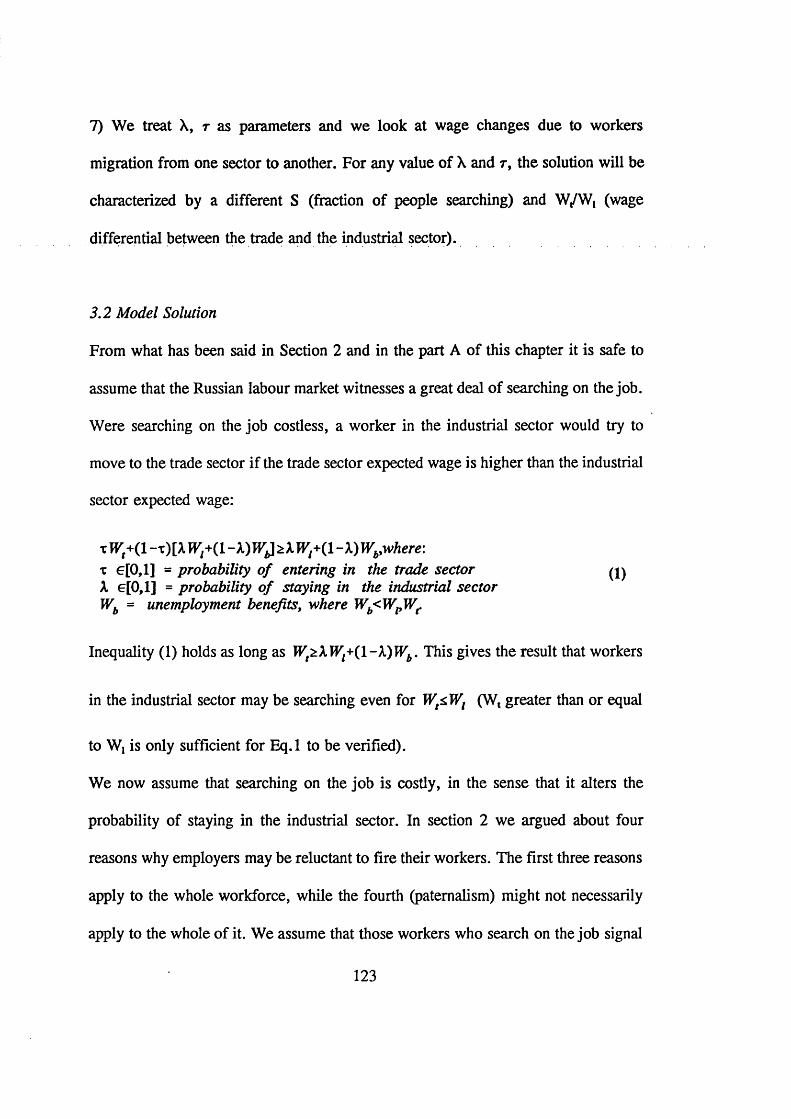
7) We treat X, r as parameters and we look at wage changes due to workers

migration from one sector to another. For any value of X and r, the solution will be

characterized by a different S (fraction of people searching) and W/W, (wage

differential between the trade and the industrial sector).

3.2 Model Solution

From what has been said in Section 2 and in the part A of this chapter it is safe to

assume that the Russian labour market witnesses a great deal of searching on the job.

Were searching on the job costless, a worker in the industrial sector would try to

move to the trade sector if the trade sector expected wage is higher than the industrial

sector expected wage:

x W+( 1 -x)[A W ^ l -X) W ^X W fQ . -X) Wpwhere:x e[0 ,l] = probability o f entering in the trade sector (1)X e[0,l] = probability o f staying in the industrial sector Wb = unemployment benefits, where Wb<WpWf

Inequality (1) holds as long as Wt^XW ^{l-X)W b. This gives the result that workers

in the industrial sector may be searching even for WtzWl (Wt greater than or equal

to W, is only sufficient for Eq.l to be verified).

We now assume that searching on the job is costly, in the sense that it alters the

probability of staying in the industrial sector. In section 2 we argued about four

reasons why employers may be reluctant to fire their workers. The first three reasons

apply to the whole workforce, while the fourth (paternalism) might not necessarily

apply to the whole of it. We assume that those workers who search on the job signal

123

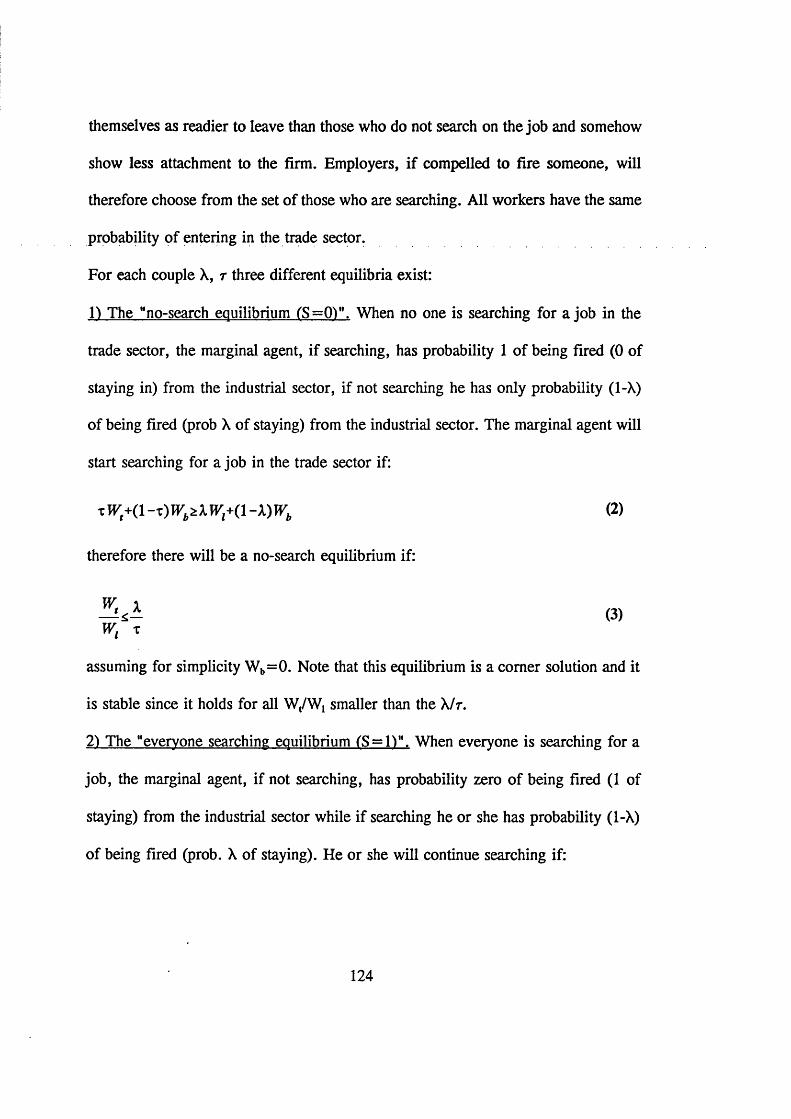
themselves as readier to leave than those who do not search on the job and somehow

show less attachment to the firm. Employers, if compelled to fire someone, will

therefore choose from the set of those who are searching. All workers have the same

probability of entering in the trade sector.

For each couple X, r three different equilibria exist:

1) The Mno-search equilibrium (S=0V'. When no one is searching for a job in the

trade sector, the marginal agent, if searching, has probability 1 of being fired ( 0 of

staying in) from the industrial sector, if not searching he has only probability (1-X)

of being fired (prob X of staying) from the industrial sector. The marginal agent will

start searching for a job in the trade sector if:

xWi+(l-x)Wb^XWl+(l-X)Wb (2)

therefore there will be a no-search equilibrium if:

W l(3)

Wt T

assuming for simplicity Wb=0. Note that this equilibrium is a comer solution and it

is stable since it holds for all W/W, smaller than the X/r.

2) The "everyone searching equilibrium (S = 1V*. When everyone is searching for a

job, the marginal agent, if not searching, has probability zero of being fired (1 of

staying) from the industrial sector while if searching he or she has probability (1-X)

of being fired (prob. X of staying). He or she will continue searching if:

124

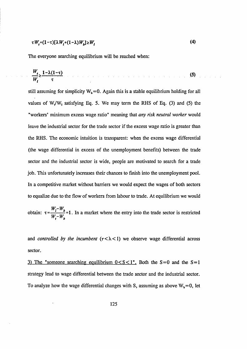
xW+(l -t)[A IV,+(1 -*) Wy ;> W, (4)

The everyone searching equilibrium will be reached when:

(5)Wt T

still assuming for simplicity Wb=0. Again this is a stable equilibrium holding for all

values of W/W, satisfying Eq. 5. We may term the RHS of Eq. (3) and (5) the

"workers’ minimum excess wage ratio” meaning that any risk neutral worker would

leave the industrial sector for the trade sector if the excess wage ratio is greater than

the RHS. The economic intuition is transparent: when the excess wage differential

(the wage differential in excess of the unemployment benefits) between the trade

sector and the industrial sector is wide, people are motivated to search for a trade

job. This unfortunately increases their chances to finish into the unemployment pool.

In a competitive market without barriers we would expect the wages of both sectors

to equalize due to the flow of workers from labour to trade. At equilibrium we would

Wr Wbobtain: x= =1. In a market where the entry into the trade sector is restricted

Wt-Wb

and controlled by the incumbent ( r< X < l) we observe wage differential across

sector.

3) The "someone searching equilibrium 0 < S < 1 M. Both the S=0 and the S = 1

strategy lead to wage differential between the trade sector and the industrial sector.

To analyze how the wage differential changes with S, assuming as above Wb=0, let

125

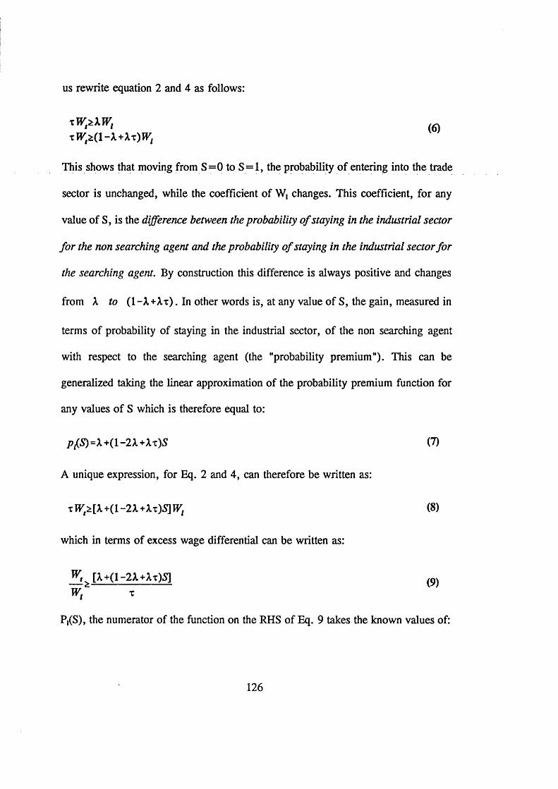
us rewrite equation 2 and 4 as follows:

t W^XWjt w ^ i - x +x^

This shows that moving from S=0 to S = l, the probability of entering into the trade

sector is unchanged, while the coefficient of W, changes. This coefficient, for any

value of S, is the difference between the probability o f staying in the industrial sector

fo r the non searching agent and the probability o f staying in the industrial sector for

the searching agent. By construction this difference is always positive and changes

from X to (1-A.+At) . In other words is, at any value of S, the gain, measured in

terms of probability of staying in the industrial sector, of the non searching agent

with respect to the searching agent (the "probability premium"). This can be

generalized taking the linear approximation of the probability premium function for

any values of S which is therefore equal to:

p£S) =X+(l-2X+Xx)S (7)

A unique expression, for Eq. 2 and 4, can therefore be written as:

t Wt7>[X +(I -2X +Xx)S1 Wt (8 )

which in terms of excess wage differential can be written as:

W ,.. [X+(1-2A.+Xt)S]

w i x

Pj(S), the numerator of the function on the RHS of Eq. 9 takes the known values of:

126

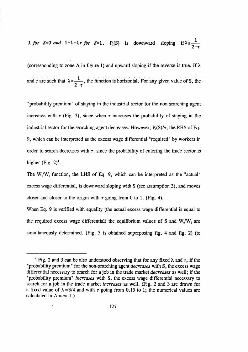
X for S=0 and 1-X+Xx for S=1. Pj(S) is downward sloping ifX ^-J—2 - t

(corresponding to zone A in figure 1) and upward sloping if the reverse is true. If X

1 ..............................................................................................and r are such that X =----- , the function is horizontal. For any given value of S, the

"probability premium” of staying in the industrial sector for the non searching agent

increases with r (Fig. 3), since when r increases the probability of staying in the

industrial sector for the searching agent decreases. However, P^SVr, the RHS of Eq.

9, which can be interpreted as the excess wage differential "required" by workers in

order to search decreases with r, since the probability of entering the trade sector is

higher (Fig. 2)4.

The Wt/W, function, the LHS of Eq. 9, which can be interpreted as the "actual"

excess wage differential, is downward sloping with S (see assumption 3), and moves

closer and closer to the origin with r going from 0 to 1. (Fig. 4).

When Eq. 9 is verified with equality (the actual excess wage differential is equal to

the required excess wage differential) the equilibrium values of S and Wt/Wj are

simultaneously determined. (Fig. 5 is obtained superposing fig. 4 and fig. 2) (to

4 Fig. 2 and 3 can be also understood observing that for any fixed X and r, if the "probability premium" for the non-searching agent decreases with S, the excess wage differential necessary to search for a job in the trade market decreases as well; if the "probability premium" increases with S, the excess wage differential necessary to search for a job in the trade market increases as well. (Fig. 2 and 3 are drawn for a fixed value of X=3/4 and with r going from 0,15 to 1; the numerical values are calculated in Annex 1.)

127

insure stability let us assume for a moment that the actual W^W, function is steeper

than P1(S)/r, the required W/Wj). Not surprisingly they depend on X and r. Generally

speaking, the higher is t , for a fixed X, the lower the excess wage differential and

the lower the equilibrium value of S.

We can have two types of solutions S < 1 (more likely the higher r is) and S = 1

(more likely the lower r is). A S < 1 solution is associated with a lower excess wage

differential than a S = 1 solution. If the Wt/W, function is less steep than the Pi(S)/r,

when t rises the equilibrium value of Wt/W, still falls, but S = 1 (comer solution)

remains the only stable equilibrium value.

Proposition 1. For any given X, the more relaxed the entry barriers to the trade

sector are, the smaller will be the equilibrium wage differential across sectors

and the fraction of people searching.

To summarize, when equation 3 is verified, no search will take place and the

equilibrium is a comer solution S =0. If equation 3 is not verified, some search will

take place and the move from the old system to transition determines an internal

equilibrium if and only if it exist an 0<S*< 1 such that Eq. 9 is verified. Finally,

when equation 4 is verified for S*=l the solution is again a comer solution and

everyone in the industrial sector is searching for a job in the trade sector.

The comer solution S=0 can be interpreted as the ossification of the "Soviet system".

The transition is only equal to an initial shock to wages with no reaction from the

side of the workers.

128

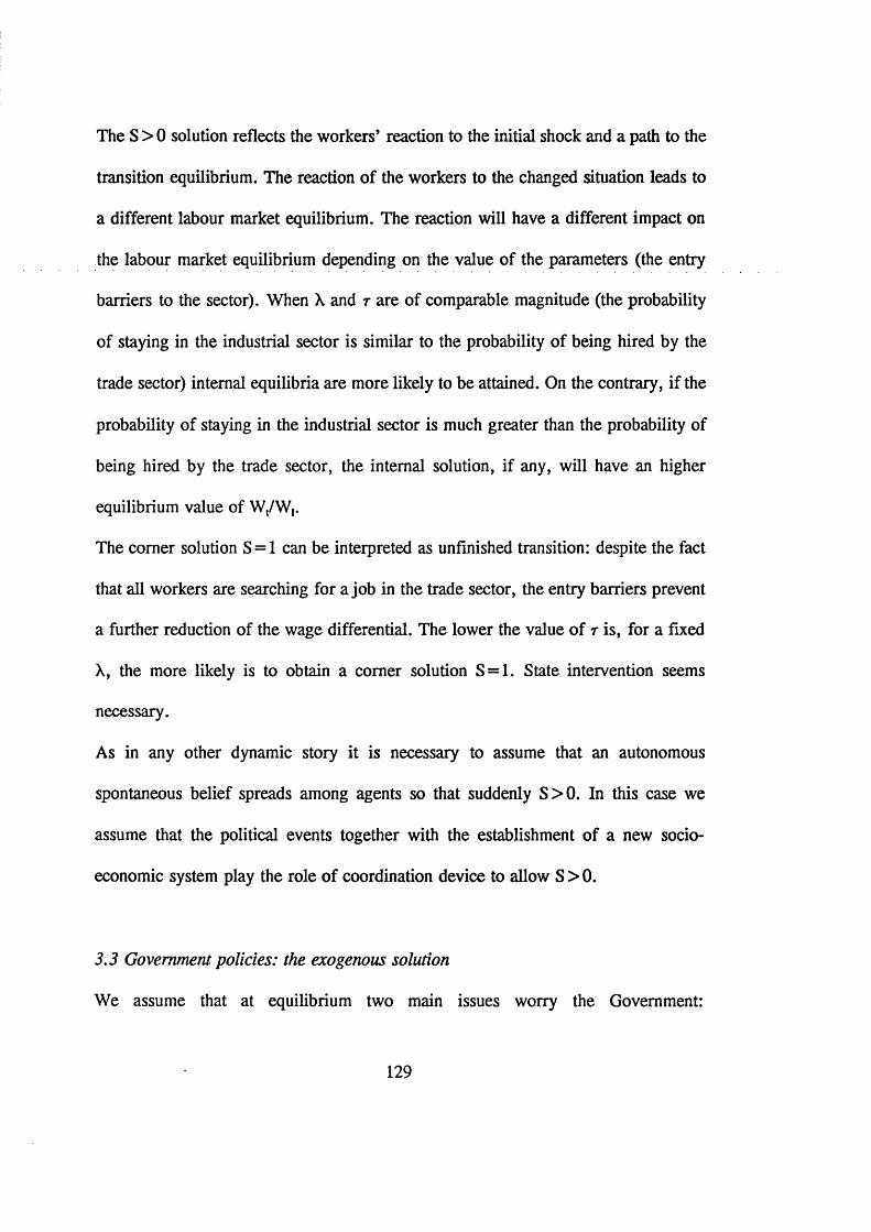
The S > 0 solution reflects the workers’ reaction to the initial shock and a path to the

transition equilibrium. The reaction of the workers to the changed situation leads to

a different labour market equilibrium. The reaction will have a different impact on

the labour market equilibrium depending on the value of the parameters (the entry

barriers to the sector). When X and r are of comparable magnitude (the probability

of staying in the industrial sector is similar to the probability of being hired by the

trade sector) internal equilibria are more likely to be attained. On the contrary, if the

probability of staying in the industrial sector is much greater than the probability of

being hired by the trade sector, the internal solution, if any, will have an higher

equilibrium value of Wt/W,.

The comer solution S = 1 can be interpreted as unfinished transition: despite the fact

that all workers are searching for a job in the trade sector, the entry barriers prevent

a further reduction of the wage differential. The lower the value of t is, for a fixed

X, the more likely is to obtain a comer solution S = l. State intervention seems

necessary.

As in any other dynamic story it is necessary to assume that an autonomous

spontaneous belief spreads among agents so that suddenly S> 0. In this case we

assume that the political events together with the establishment of a new socio­

economic system play the role of coordination device to allow S > 0.

3.3 Government policies: the exogenous solution

We assume that at equilibrium two main issues worry the Government:

129

unemployment and social cohesion. As described in the previous section some

workers have been fired from the industrial sector and have not managed to enter the

trade sector. The pool of unemployed people has therefore increased and society is

split into three main income classes: trade workers, labour workers and unemployed

workers. A reasonable Government policy is to fight unemployment and/or to keep

wage differentials within acceptable limits.

We briefly analyze two kinds of policies: administrative and market ones.

Administrative policies imply transfers from the "richer" to the "poorer" (namely to

increase unemployment benefits and eventually to allow for transfers to the industrial

sector workers). Transfers would be effective only if an efficient progressive system

of taxation were in place and workers in the trade sector would bear the largest

share. But given the current different degree of tax compliance between workers of

the trade and the industrial sector, it would not be surprising if an increased taxation

to finance social benefits would increase the gap between net incomes. Therefore to

increase social benefits would be not only ineffective but even harmful: the excess

wage differential will become even wider thus giving a greater incentive to leave the

industrial sector for the trade sector and increasing the number of unemployed

people.

Market policy options should be consistent with the other reforms implemented to

move the economy system from a command economy to a market economy. In this

particular case a Government policy should facilitate the system to reach the free-

market equilibrium and possibly full employment. This can be done in two non

130

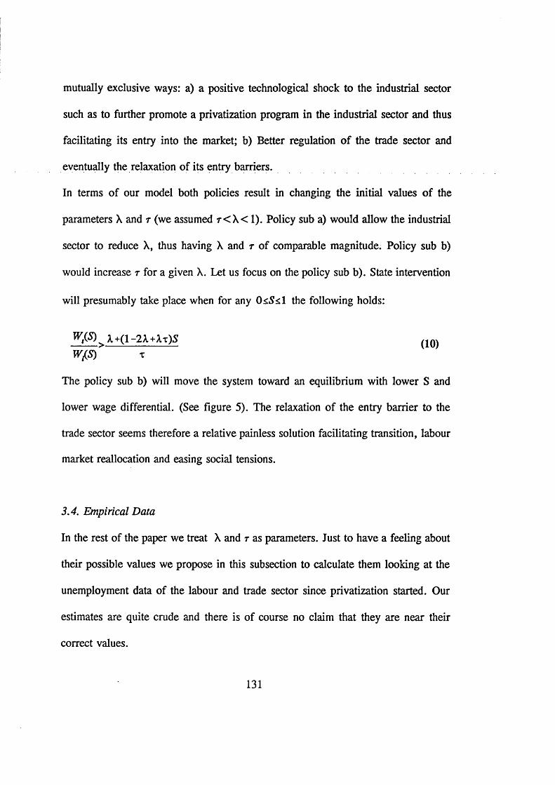
mutually exclusive ways: a) a positive technological shock to the industrial sector

such as to further promote a privatization program in the industrial sector and thus

facilitating its entry into the market; b) Better regulation of the trade sector and

eventually the relaxation of its entry barriers.

In terms of our model both policies result in changing the initial values of the

parameters X and r (we assumed r < \ < 1). Policy sub a) would allow the industrial

sector to reduce X, thus having X and r of comparable magnitude. Policy sub b)

would increase r for a given X. Let us focus on the policy sub b). State intervention

will presumably take place when for any the following holds:

wX5)^ + ( i -2A.+;it),sW/iS) T

The policy sub b) will move the system toward an equilibrium with lower S and

lower wage differential. (See figure 5). The relaxation of the entry barrier to the

trade sector seems therefore a relative painless solution facilitating transition, labour

market reallocation and easing social tensions.

3.4. Empirical Data

In the rest of the paper we treat X and r as parameters. Just to have a feeling about

their possible values we propose in this subsection to calculate them looking at the

unemployment data of the labour and trade sector since privatization started. Our

estimates are quite crude and there is of course no claim that they are near their

correct values.

131

These simulations are shown in Annex 2. Table 1 is our reduction of Table 74 in

RET 94/3/2 and Table 87 in RET 94/3/4. Under the entry "Trade" we include all

sectors (trade, catering, commercial services, health, sport, education) paying higher

wages and under the entry "Labour" we include all sectors (industry, agriculture,

transports, construction, science and public administration) paying lower wages.

Residual workers are accounted with the Trade sector.

From table 1, we calculate the series of tables 2. They give a numerical value to the

parameters of our model.

Some assumptions are needed in order to calculate X and r. To calculate X for the

period (t, t+n) we simply divide the number of workers in the industrial sector at

period (t+n) by the number of workers in the industrial sector at period t. To

calculate r (the probability of successfully entering the trade sector) we need to know

how many workers of the industrial sector searched for a job in the trade sector. We

assume that this figure is equal to k times the number of agents who finally separated

from the industrial sector; since we can indeed observe 6 (numbers of people who

entered the trade sector divided by number of people who left the industrial sector)

we therefore obtain r=0/k. Clearly, the value of k plays a crucial role and therefore

we have run the simulation for 3 different values of k. (Tables 2a to 2c). In each of

these tables the required W/W, and the "premium probability" are calculated for

three different values of S (0, 0.5, 1).

We have chosen 4 periods relevant for the analysis. One of them, 93Q1-91, (93Q1

means the first quarter of 93) has been further divided in two sub-periods.

132

Commenting on the simulations we focus on table 2b, which means to assume that

the number of workers who left the industrial sector is just one third of those who

were searching for a job in the trade sector. Let us first have a look at the column

94Q4-91 which gives an overall evaluation of labour market movements from the

starting of privatization to the most recent available data. Generally, it can be

observed that the industrial sector has been a job destructor sector throughout

transition, while the trade sector has been always (except in the period 93-93Q1) a

job creator sector. However the trade sector has not absorbed all those workers

leaving the industrial sector which has resulted in an increase in the number of

unemployed. The probability of staying in the industrial sector has kept stable over

all periods, while the probability of being hired in the trade sector has widely

fluctuated. In terms of our model, it means that in the period 94Q4-91, for a given

X and r both the excess wage differential necessary to search and the "premium

probability" decrease when going from S=0 to S = 1 (being A>1/(2-t)). The value

of required excess wage differential is quite high as a consequence of the fact that

X=.87 while 7 =. 14. (Figure 6 and 7)

In the sub-period 93Q1-92 when the highest values of 7 are observed (though

X>1/(2- t) still holds). The required excess wage ratio is relatively small. In this

period reallocation has played a major role: the trade sector has hired as many new

workers as have separated from the industrial sector.

Looking at the whole period not all the fired workers from the industrial sector are

hired by the trade sector and the average wage of the trade sector is consistently

133

greater than the average wage of the industrial sector. These two findings seem to

point to the existence of resistant entry barriers controlled by the incumbents which

prevents the equalization of average wages. Though data on the wage in the trade

sector are difficult to interpret given the great deal of underreporting for purpose of

tax evasion, it seems that, despite the new hirings over the whole period, the wage

differential across sectors did not reduce. One possible explanation, among many

others, is that the trade sector prevents its own wage to decrease by accepting new

workers only when showing increasing returns to scale and expelling workers when

showing decreasing returns to scale. At that point those who leave the industrial

sector can enter only into the unemployment pool. The equilibrium therefore is not

characterized, as usual, by the same average wage across both sectors, but is an

equilibrium with a wage differential.

3.5 The Black Sector: the endogenous solution

In the present section we look at how market forces can overcome the entry barriers

and move the system away from the equilibrium unemployment. We make the

hypothesis that Russian unemployed workers’ may enter into a third unofficial sector

termed the "black sector" which can be thought of as a sector in some way related

to the black or the grey economy5. In other words, a growing social discontent due

to the wage gap among sectors, to the growing unemployment and to the state non

5 To be precise with "black sector" we mean legal and illegal "Directly Unproductive, Profit-seeking (DUP) activities" as christened by Bhagwati (1982). This seems to fit with Russian reality.

134

implementation of adequate active policies, may lead some unemployed workers to

"privatize" themselves by joining a third unofficial sector. We assume that, social

attitudes are such that workers prefer to earn a given amount of money in any of the

regular sectors rather than in the black sector. Money earned in the black sectors, to

be comparable to money earned in any regular sector need therefore to be discounted

by a factor accounting for "moral costs". The "net wage" of the rent seeking sector

is thus the difference between M, the rent extracted from the trade sector and m, the

hmoral costs of being involved in rent-seeking activities: W =M-m= n

nmtn

where nm is the number of workers in the black sector and /x (pe[0 ,l]) the

probability of entering the black sector). This wage function is similar to the one of

the trade and industrial sector except for the r^/n variable which represents the

fraction of people in the rent-seeking sector and allows to determine moral costs. It

is standard to assume - ^ - < 0 and - ^ - < 0 to describe the decreasing marginaldnm dnmm ftx

productivity of the black sector and the negative relationship between personal moral

costs and the fraction of people working in the black sector (for a discussion, see

Cowell, 1990). Therefore it is possible to assume that for some values of the first

and the second derivative of Wm with respect to nm are positive, for some other

values of nm the first derivative is positive and the second negative and for some

135

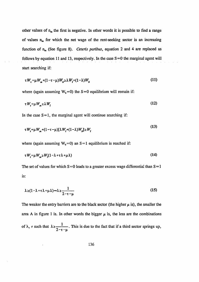
other values of nm the first is negative. In other words it is possible to find a range

of values nm for which the net wage of the rent-seeking sector is an increasing

function of (See figure 8). Ceteris paribus, equation 2 and 4 are replaced as

follows by equation 11 and 13, respectively. In the case S=0 the marginal agent will

start searching if:

xWs\LWm+ (l-x-v)W b>\Wl+{\-X)Wb (11)

where (again assuming Wb=0) the S=0 equilibrium will remain if:

xW+pWm<.XWl (12)

In the case S = l, the marginal agent will continue searching if:

(13)x\vt+\L wm+(i - t - p)[A w^+(i -X) wj wi

where (again assuming Wb=0) an S = 1 equilibrium is reached if:

xW+pWmzW£l-X+xX+\iX) (14)

The set of values for which S = 0 leads to a greater excess wage differential than S = 1

is:

A.i(l-X+Ti+(iA.)-*A.i— -— (15)2 -T -p

The weaker the entry barriers are to the black sector (the higher p is), the smaller the

area A in figure 1 is. In other words the bigger p is, the less are the combinations

of X, r such that Xz— -— . This is due to the fact that if a third sector springs up, 2 - x - p

136

the true choice is between taking the risk in the industrial sector or in the trade

sector. If the trade sector offers also outside options (the black sector) the marginal

agent is ready to risk the trade sector even if the risk is greater than in the industrial

sector (X relatively close to, but still greater than, r).

Using equation 12 and 14, the linear approximation, for 0 < S < 1, of the "premium

probability" function of staying in the industrial sector for the non-searching agent

can be calculated as:

t W 'tik +[1 -2X+X(t+vj\S}Wr \iWm (16)

With respect to the /x=0 case we have smaller intercept and greater slope. The line

of the requested minimum wage differential to move from one sector to another turns

anti-clockwise (See Figure 10).

We have carried on some calculations for the case where r=0.15, being the case of

a low r the one which gives the highest incentive to people to create a rent-seeking

sector. Three different values of p (0.20, 0.52 and 1) have been considered to

analyze the case where X z— -— is verified, the case where X<:— -— is verified2 - x - p 2 - x - p

and the borderline. A sufficient condition to obtain the anti-clockwise movements is

simply Wm>W,. For any value of S the equilibrium value of the excess wage

differential (between the labour and the trade market) is smaller when p > 0. (Figure

10 and the last table of annex 3). The existence of the rent-seeking sector gives a

further incentive for people to search. Comer solutions become more likely. For any

137

0 < S < 1 the interpretation is transparent: the existence of a third sector allows for

equilibria with a smaller wage differential between the trade and the industrial sector.

It means that the existence o f a third sector increases the outflow o f workers from the

industrial sector under each strategy. Some will enter the trade sector, some the

unemployment pool and some the black sector. The wage will increase in the labour

and in the black sector and decrease in the trade sector. At equilibrium we will

observe a high Wm and low Wt and W, (eventually for X smaller than r, Wt could be

smaller than W,). Indeed, the value of Wt, as argued by Shleifer and Vishny (1992

and 1993), depends negatively on the number of people in DUP activities. This will

be the logical result of an increasing number of "Directly Unproductive and Profit-

Seeking" agents.

Proposition 2: The existence of the rent seeking sector paying net wages

increasing with the number of workers (at least for some values of nm) crowds

out both the trade and the industrial sector. Ceteris paribus, for any internal

equilibrium, the value of S will be higher and the value of Wt/W, lower than in

the no-rent-seeking case. The final equilibrium may be such that Wm>WfiWr

The entry barriers to the trade sector, as a way to keep wages high, have been proved

not only ineffective, but also harmful. Since entry barriers existed, a rent-seeking

sector developed, leading in turn to the reduction of wages in the trade sector.

This new equilibrium implies even more unemployment than in a standard Harris-

Todaro situation. Endogenous market forces, coupled with a weak institutional

framework, may overcome entry barriers through DUP activities and reach an even

worse unemployment equilibrium. The DUP sector drags resources from the most

productive sector thus reducing the effectiveness of entry barriers to the trade sector

as a mean to keep trade wages higher. Any legal sector could not nullify the effect

of entry barriers unless it proves able to pay higher wages than the trade sector. This

makes the rising of a DUP sector more likely than the rising of any other legal

sector. This process could even enter in a vicious circle such that DUP activities

reduce to zero legal productive activity and the whole system is just a society of DUP

persons.

Policy conclusions are self-evident. The most likely reaction of the market to a device

(entry barriers) which allows a sector to be protected is another device (DUP

activities) which somehow mitigates or annuls the effects of the first device. In other

words in the absence of any exogenous intervention (as one of those advocated in

section 3.3) or any exogenous technological shock to the industrial sector a DUP

sector will become the strongest of the market.

3.6: The Black Sector hysterisis

The exogenous and endogenous solutions as they were presented in sections 3.3 and

3.5 respectively, seem two most likely outcomes for the Russian economy. Let us

assume that in the short run the Government decides not to intervene and therefore

the economy goes towards the so-called endogenous solution. Given that the

Government cannot consider it as a satisfactory outcome, what are the policy options

left to it rid the economy of the rent-seeking sector? In other words, at that stage can

139

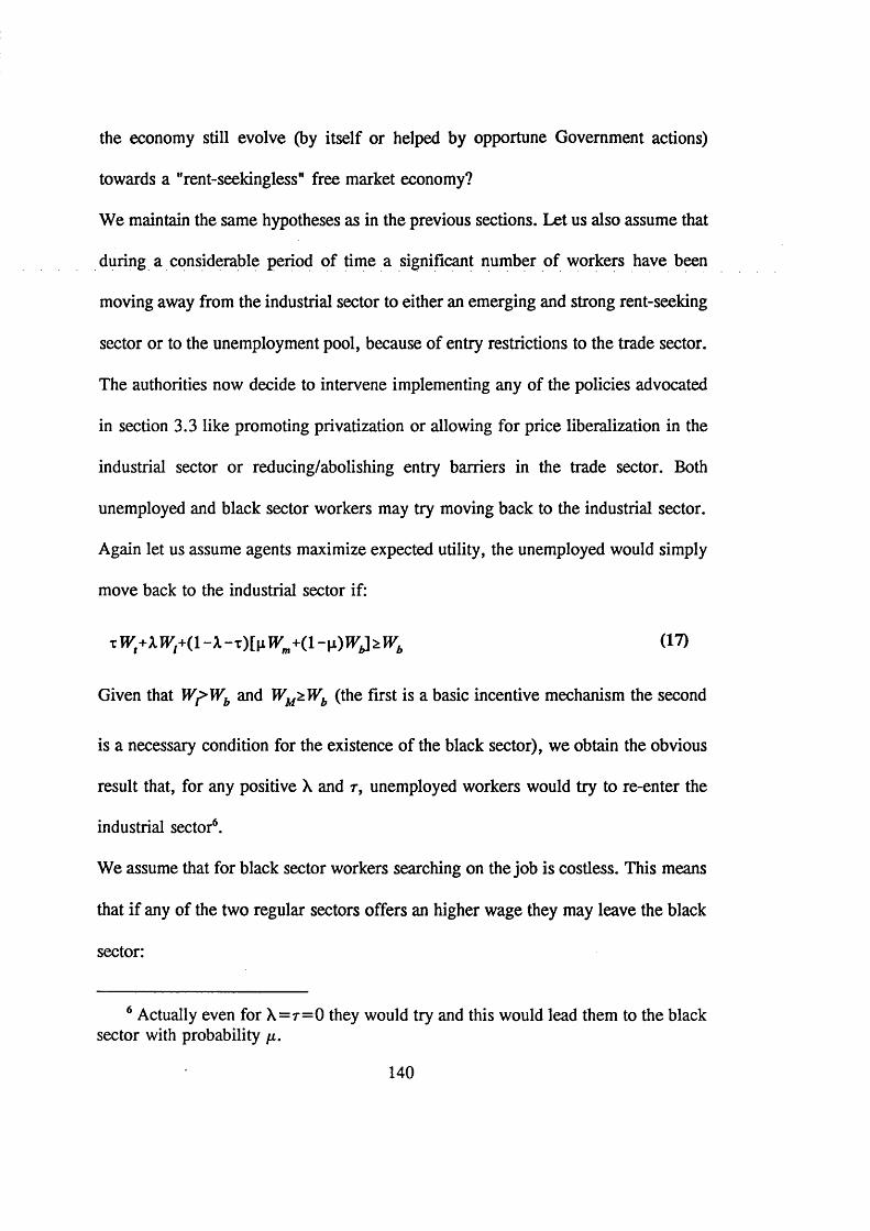
the economy still evolve (by itself or helped by opportune Government actions)

towards a "rent-seekingless" free market economy?

We maintain the same hypotheses as in the previous sections. Let us also assume that

during a considerable period of time a significant number of workers have been

moving away from the industrial sector to either an emerging and strong rent-seeking

sector or to the unemployment pool, because of entry restrictions to the trade sector.

The authorities now decide to intervene implementing any of the policies advocated

in section 3.3 like promoting privatization or allowing for price liberalization in the

industrial sector or reducing/abolishing entry barriers in the trade sector. Both

unemployed and black sector workers may try moving back to the industrial sector.

Again let us assume agents maximize expected utility, the unemployed would simply

move back to the industrial sector if:

xW +\W l+ (\-\-x)l\LW m+ (l-\L )W ^W b (17)

Given that W^Wb and WM Wb (the first is a basic incentive mechanism the second

is a necessary condition for the existence of the black sector), we obtain the obvious

result that, for any positive X and r, unemployed workers would try to re-enter the

industrial sector6.

We assume that for black sector workers searching on the job is costless. This means

that if any of the two regular sectors offers an higher wage they may leave the black

sector:

6 Actually even for X=r=0 they would try and this would lead them to the black sector with probability p.

140

xWt+\Wl+ {\-\-i)W b*Wm (18)

A necessary conditions for Eq. (18) to be verified is Wl'tWm or Wt*Wm.

Figure 8 shows that:

for nm<nm, the equilibrium-wage o f the rent-seeldng sector is Wm=0,

for nOT>»^, the equilibrium-wage o f the rent-seeking sector is Wm=Wl>§

Ceteris paribus, Eq. (18) is surely verified if n < n ’m (where n’m is the unstable

equilibrium depicted in fig. 8). In the framework of our model it means that time

matters. The more people get involved in rent-seeking activities, the lower moral

costs are and the greater the wage of the industrial sector needs to be to motivate

people to try leaving the black for the industrial sector. If the size of the black sector

is less than n’m the system may come back to a no black sector equilibrium, otherwise

the black sector will remain in the economy. This dichotomy in the pattern of the

black sector can be justified by thinking of an initial group of "amoral" people who

would always go for black sector activities. Once this original group gets bigger,

"moral" people revert to black sector activities since moral costs are very much

lower.

As pointed out in section 3.5, this is due to the standard assumption that moral costs

m depend negatively on the fraction of people into the black sector.

Proposition 3: privatization of the industrial sector and/or abolition of entry

barriers to the trade sector would prevent the black sector appearing. However

141

once the black sector (rent-seeking) has appeared and has developed the same

Government policies might not be enough to rid it from society.

This conclusion could be strengthened by introducing into the model the workers’ loss

of human capital deriving from a period of unemployment or black-sector activities

which would reduce productivity, and in turn their per capita wage once they move

back to any of the two regular sector.

4. Conclusions

We have presented a model aiming to describe the changes in the labour market in

Russia during the transition from a command to a market economy. The USSR had

an overregulate and substantially egalitarian labour market, while Russia has a very

unequal and differentiated labour market. We argued that is due to the fact that

transition affected different productive sectors in different ways. The trade sector

reformed much more quickly and more effectively than the industrial sector. Workers

of the trade sector enjoy higher wages than those of the industrial sector. Workers

tend to move away from the industrial sector toward the trade sector attracted by

large wage differentials. At equilibrium the wage differential and the number of

people who search for a job will depend on the hiring and firing probability of both

sectors.

Employment data show that the industrial sector, in need of deep restructuring, has

consistently been a job destructing sector since privatization started; the trade sector

has been job creator, but not enough to absorb all the workers leaving the industrial

142

sector. The wage differential does not seem reduced which therefore points to the

existence of some entry barriers. A large and non-reducing wage differential is a

source of social tension and of instability of the current equilibrium. We have argued

that Government policies should try to close the wage gap, bringing the Russian

system close to a competitive market economy where barriers are very much reduced.

Indeed, Government policies should facilitate a market solution through the

completion of the privatization program for the industrial sector and the relaxation

of the entry barriers to the trade sector. In the absence of these, we have argued that

a black sector might eventually appear and develop offering a better alternative to

unemployment. The black economy might become the real antagonist to the trade

sector. This, in turn, would increase the pressure for Government intervention. We

have also shown that once the black sector has developed, further privatization of the

industrial sector and/or abolition of the entry barriers to the trade sector may not be

enough to free society of the black sector.

143

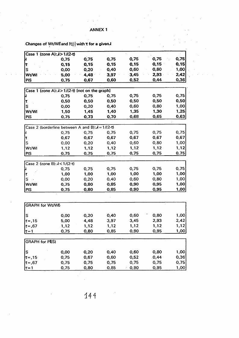
ANNEX 1

Changes of Wt/WEand P£(s) with ! for a given^l

Case 1 (zone A):>01/(2-t) \ 0,75 0,75 0,75 0,75 0,75 0,75t 0,15 0,15 0,15 0,15 0,15 0,15S 0,00 0,20 0,40 0,60 0,80 1,00Wt/WI 5,00 4 ,48 3,97 3,45 2,93 2,42PIS 0,75 0,67 0,60 0,52 0,44 0,36

Case 1 (zone A):^>1/(2-T) [not on the graph]4 0,75 0,75 0,75 0,75 0,75 0,75T 0,50 0.50 0,50 0,50 0.50 0,50S 0,00 0,20 0,40 0,60 0,80 1,00Wt/WI 1,50 1.45 1,40 1,35 1.30 1.25PIS 0.75 0,73 0,70 0.68 0,65 0,63

Case 2 (borderline between A and B):/l = 1 /(2-T)4 0,75 0,75 0,75 0,75 0,75 0,75T 0.67 0,67 0,67 0.67 0.67 0.67S 0,00 0,20 0,40 0,60 0,80 1,00Wt/WI 1,12 1.12 1.12 1,12 1.12 1.12PIS 0,75 0,75 0.75 0,75 0,75 0,75

Case 2 (zone B):/I<1/(2-t)4 0,75 0,75 0,75 0,75 0,75 0,75T 1.00 1,00 1,00 1,00 1.00 1,00S 0,00 0,20 0,40 0,60 0,80 1,00Wt/WI 0,75 0.80 0,85 0,90 0,95 1,00PIS 0,75 0.80 0,85 0.90 0,95 1,00

GRAPH for Wt/Wfc

S 0,00 0 ,20 0,40 0,60 ‘ 0 ,80 1,00r = , i 5 5,00 4,48 3,97 3,45 2,93 2,42T=,67 1.12 1,12 1,12 1,12 1,12 1,12T = 1 0,75 0,80 0,85 0,90 0,95 1,00

GRAPH for PKS)

S 0,00 0,20 0,40 0,60 0,80 1,00T=,15 0,75 0,67 0,60 0,52 0,44 0,36T = ,67 0,75 0,75 0,75 0,75 0,75 0,75T= 1 0,75 0,80 0,85 0,90 0,95 1,00

4 4 4

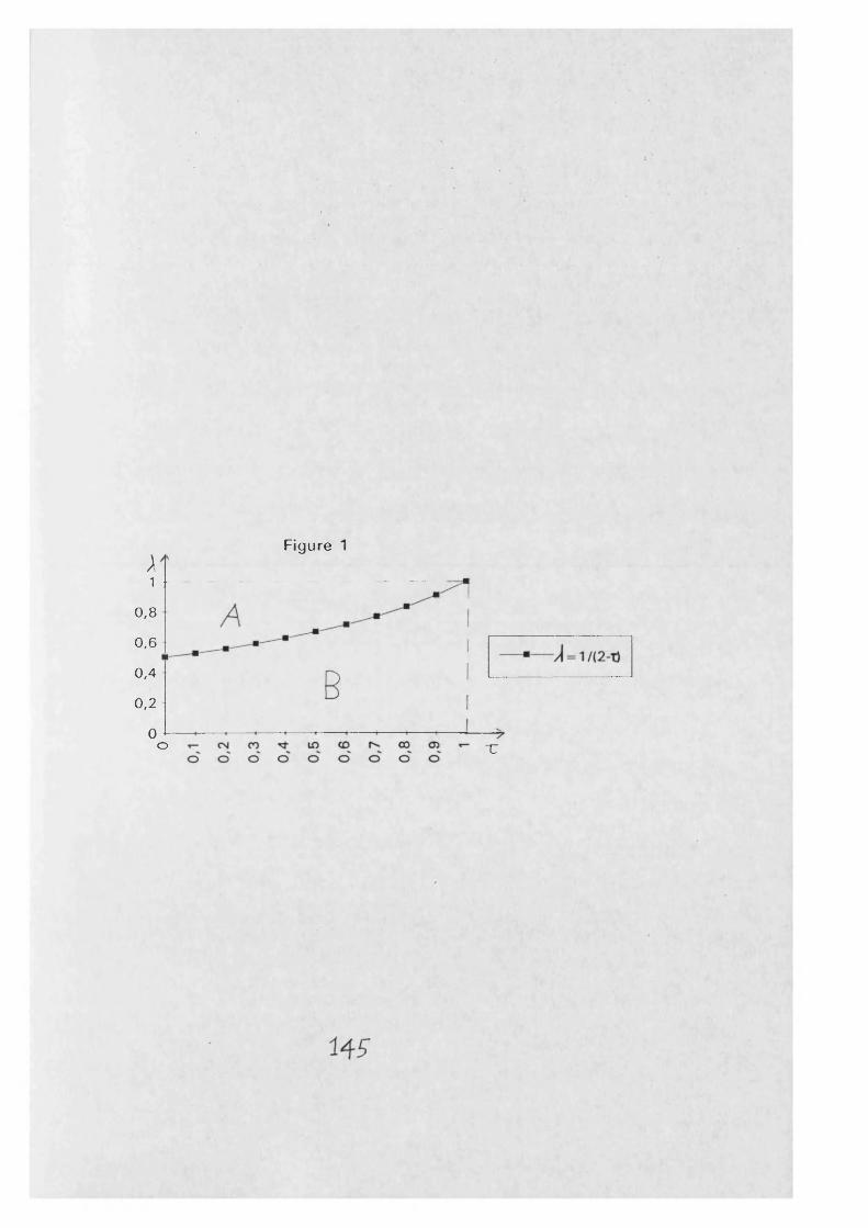
Figure 1x1

0,8

0,6

0,4

0,2

0o X

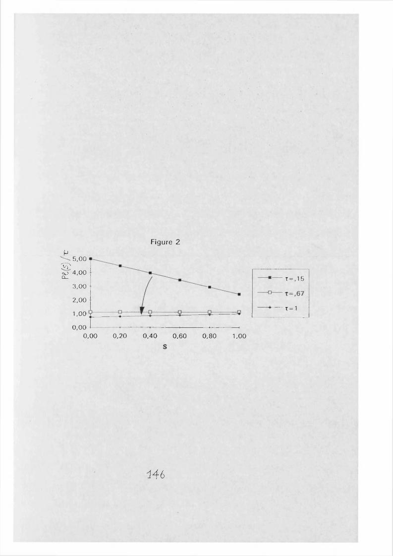
Figure 2P

^ 5,00SD^ 4 ,00Q_

3,00

2,00

1,00

0,000,00 0,20 0 ,40 0 ,60 0,80 1,00

T = ,1 5

T = 1

146

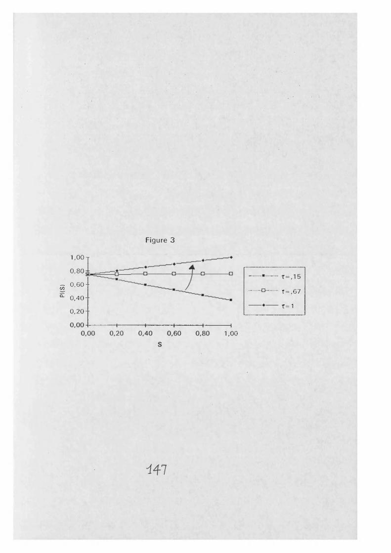
PI(S

)

Figure 3

1,00 T

0.80

0,60--

0 ,40 - •

0 , 2 0 -

t = ,67

T = 1

1,00

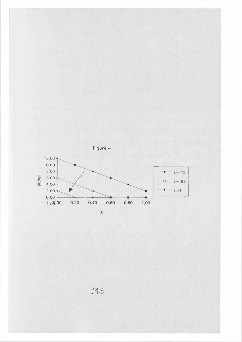
Figure 4

12,00 10,00

8,00 6,004.002.00 0,00

-2 ,0 $ ' ° °

t = 1

s

14

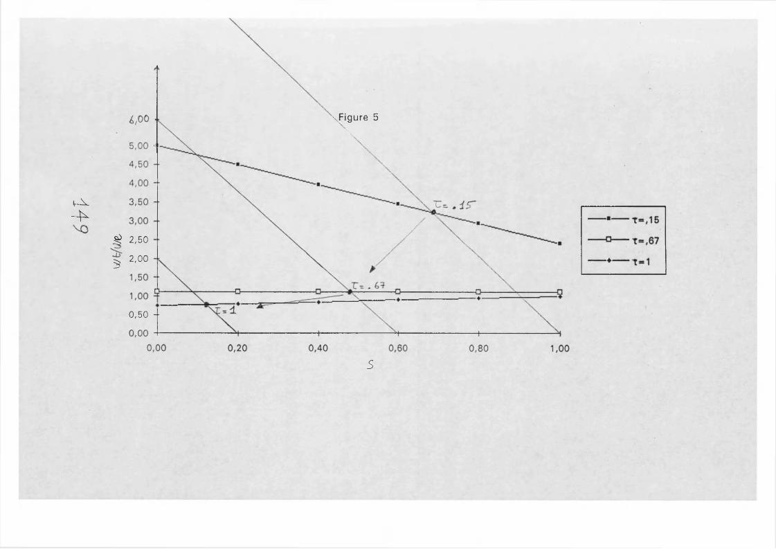
V-X■ >

\Figure 5\

^ 2,50

5 2,00

0,50 -

5

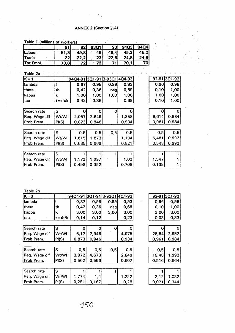
ANNEX 2 (Section 3.4)

Table 1 (millions of workers)91 92 93Q1 93 94Q3 94Q4

Labour 51,8 49 ,8 49 48,4 45,3 45,2Trade 22 22,2 23 22,6 24,8 24,8Tot Empl. 73,8 72 72 71 70,1 70

Table 2aK= 1 94Q4-91 3Q1-91 3-93Q1 4Q4-93lambdathetakappatau

\thkt= th /k

0,870,421,000,42

0,950,361,000,36

0,99neg

1,00

0,930,691,000,69

92-91 3Q1-920,960,101,000,10

0,981,001,001,00

Search rate S 0 0 0 0Req. Wage dif Wt/WI 2,057 2,649 1,358Prob Prem. PKS) 0,873 0,946 0,934

0 09,614 0,9840,961 0,984

Search rate S 0,5 0,5 0,5 0,5Req. Wage dif Wt/WI 1,615 1,873 1,194Prob Prem. PKS) 0,685 0,669 0,821

0,5 0,55,481 0,9920,548 0,992

Search rate S 1 1 1 1Req. Wage dif Wt/WI 1,173 1,097 1,03Prob Prem. PKS) 0,498 0,392 0,708

1 11,347 10,135 1

Table 2bK = 3 94Q4-91 3Q1-91 3-93Q1 4Q4-93lambdathetakappatau

\thkT=th/k

0,870,423,000,14

0,950,363,000,12

0,99neg

3,00

0,930,693,000,23

92-91 3Q1-920,960,103,000,03

0,981,003,000,33

Search rate S 0 0 0 0Req. Wage dif Wt/WI 6,17 7,946 4,075Prob Prem. PKS) 0,873 0,946 0,934

0 028,84 2,9520,961 0,984

Search rate S 0,5 0,5 0,5 0,5Req. Wage dif Wt/WI 3,972 4,673 2,649Prob Prem. PKS) 0,562 0,556 0,607

0,5 0,515,48 1,9920,516 0,664

Search rate S 1 1 1 1Req. Wage dif Wt/WI 1,774 1,4 1,222Prob Prem. PKS) 0,251 0,167 0,28

1 12,12 1,032

0,071 0,344

150

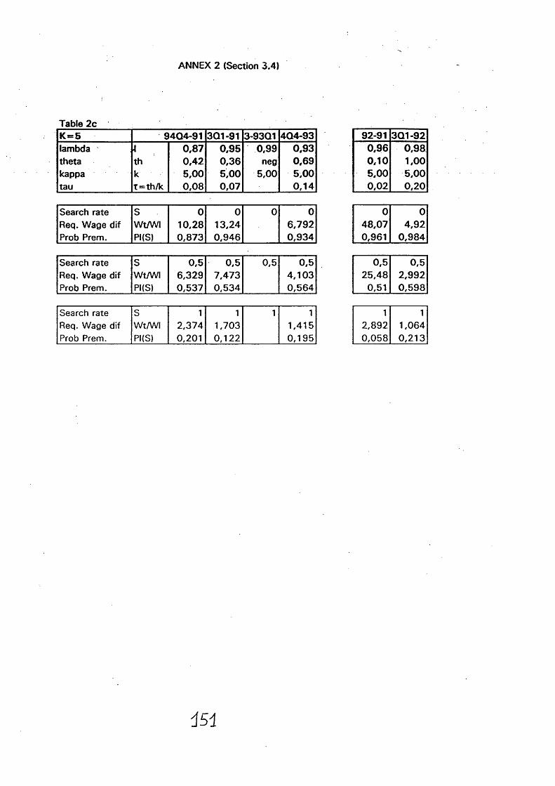
ANNEX 2 (Section 3.4)

Table 2cu>II54 94Q4-91 3Q1-91 3-93Q1 4Q4-93lambdathetakappatau

\thkT=th/k

0,870,425,000,08

0,950,365,000,07

0,99neg

5,00

0,930,695,000,14

92-91 3Q1-920,960,105,000,02

0,981,005,000,20

Search rate S 0 0 0 0Req. Wage dif Wt/WI 10,28 13,24 6,792Prob Prem. PKS) 0,873 0,946 0,934

0 048,07 4,920,961 0,984

Search rate S 0,5 0,5 0,5 0,5Req. Wage dif Wt/WI 6,329 7,473 4,103Prob Prem. PKS) 0,537 0,534 0,564

0,5 0,525,48 2,992

0,51 0,598

Search rate S 1 1 1 1Req. Wage dif Wt/WI 2,374 1,703 1,415Prob Prem. PKS) 0,201 0,122 0,195

1 12,892 1,0640,058 0,213

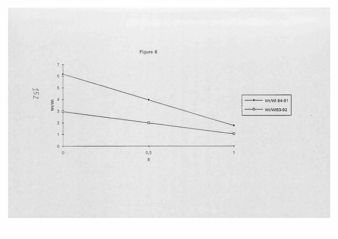
Figure 6

V-X

g£

0,5

S

Wt/WI 94-91

Wt/WI93-92

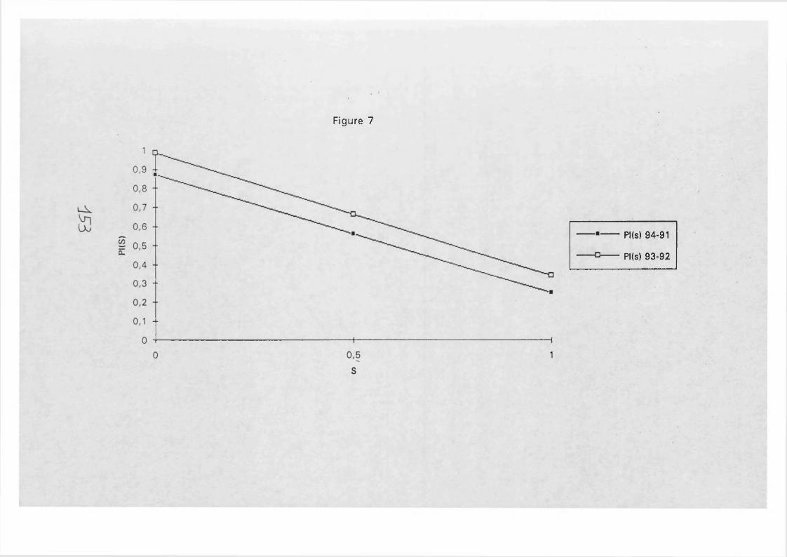
Figure 7

Pl(s) 94-91

Pl(s) 93-92

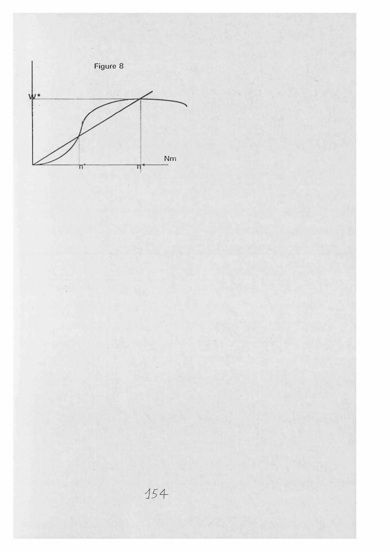
Figure 8

Nm

454-

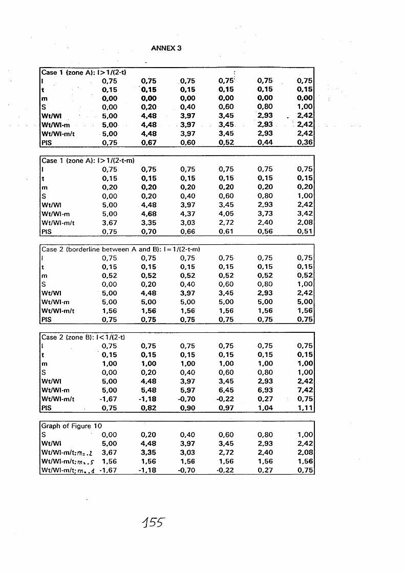
ANNEX 3

Case 1 (zone A): I

I > 1 /<2-t) 0,75 0,75 0,75 0,75' 0 ,75 0,75

t 0,15 0.15 0,15 0,15 0,15 0,15m 0,00 0,00 0,00 0,00 0,00 0 ,00S 0,00 0,20 0,40 0,60 0,80 1,00Wt/WI 5,00 4,48 3,97 3,45 2,93 . 2 ,42Wt/WI-m 5,00 4,48 3,97 3,45 2,93 2 ,42Wt/WI-m/t 5,00 4 ,48 3,97 3,45 2,93 2,42PIS 0,75 0,67 0,60 0,52 0,44 0,36

Case 1 (zone A): I

l> 1/(2-t-m) 0,75 0,75 0,75 0,75 0,75 0,75

t 0,15 0,15 0,15 0,15 0,15 0,15m 0,20 0,20 0,20 0,20 0,20 0,20S 0,00 0,20 0,40 0,60 0,80 1,00Wt/WI 5,00 4,48 3,97 3.45 2.93 2,42Wt/WI-m 5,00 4,68 4,37 4.05 3,73 3,42Wt/WI-m/t 3,67 3.35 3,03 2.72 2,40 2.08PIS 0,75 0,70 0,66 0,61 0,56 0,51

Case 2 (borderline between A and B): I = 1 /(2-t-m)I 0,75 0,75 0,75 0,75 0,75 0,75t 0,15 0,15 0.15 0,15 0,15 0,15m 0,52 0,52 0,52 0,52 0,52 0,52S 0,00 0,20 0,40 0,60 0,80 1,00Wt/WI 5,00 4,48 3,97 3,45 2,93 2,42Wt/WI-m 5,00 5.00 5,00 5.00 5,00 5,00Wt/WI-m/t 1,56 1,56 1,56 1,56 1,56 1,56PIS 0,75 0,75 0,75 0.75 0,75 0,75

Case 2 (zone B): I

I < 1 /(2-t) 0,75 0,75 0,75 0,75 0,75 0,75

t 0,15 0,15 0.15 0,15 0.15 0,15m 1,00 1,00 1,00 1,00 1.00 1,00S 0,00 0,20 0,40 0,60 0,80 1,00Wt/WI 5,00 4,48 3,97 3,45 2,93 2,42Wt/WI-m 5,00 5,48 5.97 6.45 6,93 7 ,42Wt/WI-m/t -1,67 -1,18 -0,70 -0,22 0.27 0,75PIS 0,75 0,82 0,90 0,97 1.04 1,11

Graph of Figure 10S 0,00 0,20 0,40 0,60 0,80 1,00Wt/WI 5,00 4,48 3.97 3,45 2.93 2,42Wt/WI-m/t; m= .1 3,67 3,35 3,03 2,72 2.40 2,08Wt/WI-m/t; m », r 1.56 1,56 1.56 1.56 1,56 1,56Wt/WI-m/t; .4 -1,67 -1,18 -0,70 -0,22 0,27 0,75

455

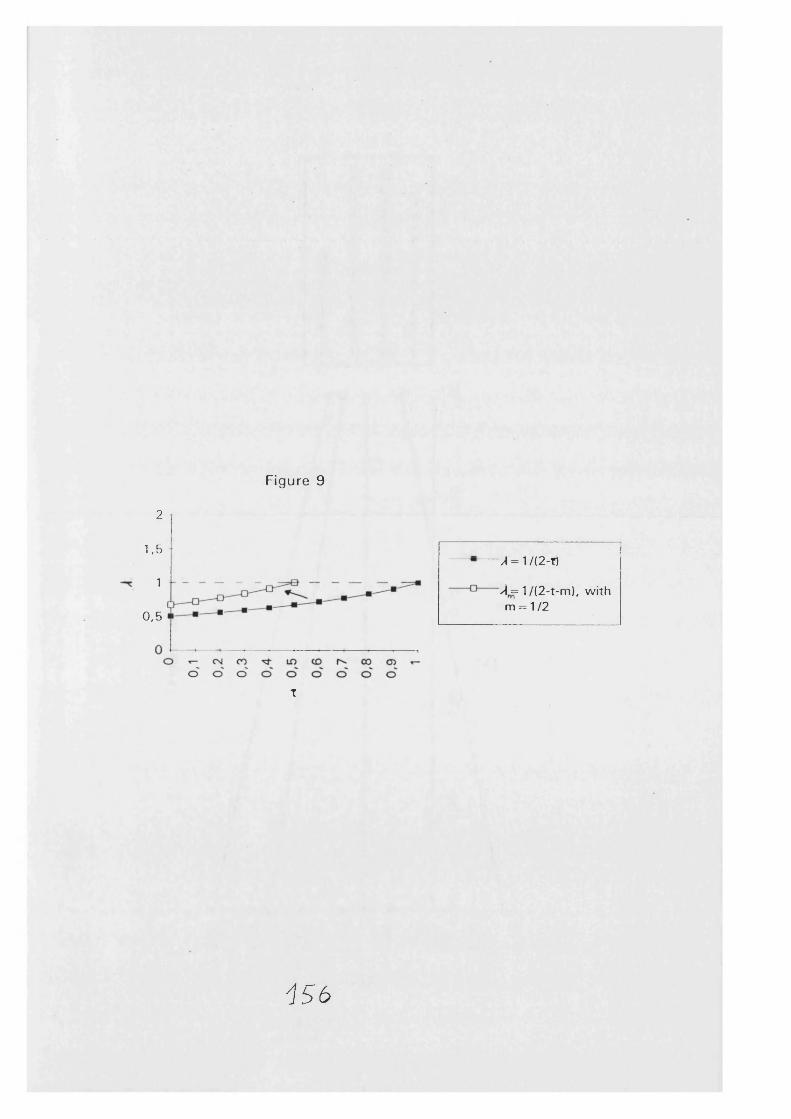
Figure 9

2

1,5

1

0,5

A = M(2-t\

A = 1/(2-t-m), with m = 1/2

T

156

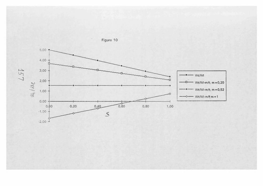
151

Figure 10

5,00 ■

- 1,00 -

- 2,00

w t/w i

Wt/WI-m/T; m=0,20

Wt/WI-m/t; m =0,52

-0 Wt/WI-m/t;-m = 1

References

Aslund, A. (ed.), 1995, "Russian Economic Reform at Risk", Pinter Publishers, London and New York.

Bhagwati, J.N., 1982, "Directly Unproductive, Profit-Seeking (DUP) Activities", Journal of Political Economy, vol 90, 5, 988-1002.

Harris, J.R. and M.P. Todaro, 1970, "Migration, Unemployment and Development: A Two Sector Analysis", American Economic Review, 60, 126-142.

Komai, J., 1979, "Resource vs Demand-constrained System", Econometrica, vol 47, 4, 801-819.

Krueger, A., 1974, "The political Economy of the Rent seeking Society", American Economic Review, 64, 291-303.

McKay, R. (ed), 1991, "Letters to Gorbachev-Life in Russia Through the Postbag of Argumenty i Fakty", Michael Joseph, London.

OECD Economic Survey, "The Russian Federation", September 1995.

Remnick, D., 1993, Lenin’s Tomb, John Wiley and Son, New York.

Roxborough, W.I. and J. Shapiro, 1994, "Excess Wage Tax", Socio-Economic Survey, Nol7, p.9, Macroeconomics and Finance Unit, Moscow.

Russian Economic Trends (RET), Government of The Russian Federation, Whurr Publishers Ltd, London (1993, 1994 and 1995 issues).

Shleifer, A. and R. Vishny, 1992, "Pervasive Shortage under Socialism", Rand Journal of Economics, XXIII, 237-46.

Shleifer, A. and R. Vishny, 1993, "Corruption", Quarterly Journal of Economics, CVIII, 599-617.

Tullock, G., 1967, "The Welfare Costs of Tariffs, Monopolies and Theft", Western Economic Journal, 5, 224-32.

Weitzman, M.L., 1977, Is the Price System or Rationing More Effective in Getting a Commodity to Those Who Need it Most", 8, 517-524.

Weitzman, M.L., 1984, "The Share Economy: Conquering Stagflation", Cambridge, Mass. Harvard University Press.

158

Conclusions

Writing the conclusions of a four-year long thesis is a sad occurrence. To minimize

the trouble I will keep them short. This last chapter is constructed as follows. Section

1 gives a brief summary of the topics explored, highlighting the results we achieved.

Section 2 deals with the limits and the shortcomings of our analysis and hints to our

future paths of research. Section 3 has the ambitious task to point out the "big

insights" I got from writing this thesis.

1. Summary

Each chapter of this thesis has dealt with the role of the state under different

circumstances. We started from a fairly traditional approach to the theory of optimal

taxation (chapter 1), we moved later to the analysis of the challenges posed by tax

evasion (chapters 2 and 3) and we concluded with the policy options left to the state

when straining through the transition from Central Planning to the Market (chapters

4 and 5). In all chapters we have taken a pure micro-economic approach looking at

how agents’ reactions to a given state policy determine the final equilibrium.

OPTIMAL TAXATION. Dealing with the theory of optimal taxation, we sought

extensions of the main results to the most realistic case of non linear income and

linear commodity taxes. In other words we have allowed the state to discriminate

income taxation across agents and to discriminate commodity taxation only across

159

goods, which is the most widespread case in reality.

We have aimed to add three pieces to the theory of taxation. First, we devised an

efficient rule for the setting of commodity taxes differentiated across goods. Second,

we have augmented the standard income tax rules by considerations aiming to offset,

at least partially, the distortions introduced by commodity taxation. Such a result is

quite encouraging for taxation theory since it implies that distortions created by an

additional instrument can be mitigated by proper adaptation of the existing

instruments. Boosted by this results we have explored whether this principle could

be fruitfully extended to the provision of public goods. As a third result we have

proved that the distortion introduced by commodity taxation to provision of public

goods vanishes under the same conditions which make the distortion introduced by

income taxation to vanish (more precisely, by the Government’s imperfect

information on agents’s type when levying income taxation). This clearly extends the

robustness of the second result and supports the use of more than one tax instrument.

In other words, in the framework of a standard model, we have been able to show

that commodity taxation can usefully supplement income taxation without necessarily

creating additional distortions.

TAX EVASION. Taking stock of the results of this first chapter, we have extended

in the second and in the third chapter our analysis to the case of commodity taxation

when tax evasion is possible. We tried to give an answer to the following questions:

is there a commodity tax structure more honesty enforcing than others? What are the

160

implications in terms of integrity and efficiency of the tax system of a change from

ad valorem taxes to value added taxes?

In the second chapter we have illustrated the historical development and the state of

the art of the tax evasion literature arguing that its development has followed two

main approaches: the taxpayer’s viewpoint approach and the social viewpoint

approach. The former approach is substantially an exercise of utility maximization

under uncertainty, the latter is a refinement of the Mirrlees-Stiglitz equation for

optimal income taxation and of the Ramsey equation for optimal commodity taxation,

respectively. Neither of the two approaches is suitable to describe the effects of a

change from one tax structure to another and therefore to answer any of the questions

raised above.

The model presented in the third chapter aims precisely to provide us with the

answers to the above-mentioned questions. Our model is different from a typical

model in the tax evasion literature since it does not seek to maximize a given tax

structure, but it looks at the effects of a change from one tax structure (ad valorem

tax) to another (value added tax). This type of reform is empirically very relevant,

since the existence of the value added tax is a prerequisite for candidate countries to

join the European Union. This requirement is usually justified, from an economic

point of view, on the production efficiency ground since VAT, allowing inputs to

enter the production function free of taxes, is neutral with respect to production

decisions. Our aim has been to show that this requirement has also a justification in

terms of fiscal policy.

161

Two parallel markets, a black and a regular one, are described. Both the black and

the regular market are divided into 3 stages of production: raw material, intermediate

good and final good. We first have shown that a VAT system unequivocally increases

the integrity of the tax system (i.e. the fraction of people operating in the regular

market rather than in the black one) and second that the efficiency of the tax system

(i.e. the total tax revenues collected) is a direct function of its integrity. Finally, as

a passing result, we have proved that a tax reform from add valorem commodity

taxation to value added taxation is a welfare improvement for the "ever-honestM

consumers since more goods are available at a lower price. The efficacy of the

reform in fighting tax evasion (both in terms of number of agents and of volume of

revenues) is a direct function of the amplitude of the reform. When the VAT system

is introduced at all stages of the production the effect is maximum, but even a partial

reform is effective.

TRANSITION ECONOMY. The transition from a command to a market economy

poses to the Government, different, and arguably greater, challenges than those of

a standard market economy. Looking at the transition from the USSR to Russia one

observes among other things that production has collapsed, shortage has almost

disappeared and unemployment has only very moderately increased.

In the fourth chapter we have tried to explain the apparent paradox of "less

production and less shortage". Before transition began, there were two, apparently

opposite, forecasts on the effects of privatization on the economic system. One

162

argued that, since firms are only producing to fulfill (or over-fulfill) the plan,

privatization will lead to a great fall of the GDP. The other argues that since firms

could not keep profits, they were artificially under-producing in order to create

shortage, thus being able to extract bribes. Once transition began, widespread

privatization has allowed for profits appropriation. This has made agents adopt a

profit maximizing behaviour. It means that loss-making firms have shut down, while

profit-making firms have started producing at the optimal point. Both forecasts were

correct, simply they applied to two mutually exclusive subsets of firms: those firms

having production entirely determined by the plan, and those firms having some

degree of freedom in choosing their production level. Typically, industrial firms

belonged to the first subset and were loss-making, while service firms belonged to

the second one and were profit-making. The closure of many industrial firms has

therefore contributed to the reduction in total production, while the expansion of the

firms in the service sectors (namely trade and distribution) has contributed to the

shortage reduction.

In the fifth chapter we have presented a model of the labour market in transition

aiming to describe the path from a full-employment with no search equilibrium (the

USSR) to a new equilibrium with unemployment and search (Russia). Using a two-

sector model where wages are a function of the sector productivity we have modelled

the equilibrium unemployment and wage differential across sectors. They depend on

the relative strength of the entry and exit barriers for workers into and from the two

sectors. Both an internal equilibrium (a fraction of people searching) and a comer

163

solution (all people searching) are possible. The stronger the entry barriers are to the

most productive sector the higher is the wage differential among sectors. In terms of

policy options we have argued that a prompt state intervention relaxing entry barriers

to the most productive sectors would be the most appropriate measure. We have

showed that, under some standard conditions in terms of moral costs, if a rent-

seeking sector appears, wage differential across sectors will decrease and search will

increase. The rent-seeking sector might become the viable alternative to

unemployment and underemployment. The long term existence of a rent-seeking

sector is guaranteed once the sector has reached a critical mass. At that point, though

the existence of a rent-seeking sector would have increased the pressure for state

intervention, the above mentioned state policies are not sufficient to free society of

the rent-seeking sector, which means that for policy implications time matters.

2. Limits and Shortcomings

The aim of this section is not to give a list of all the conceivable limitations of each

of the three models we have used. Limitations and shortcomings are necessarily many

and they are a consequence of the assumptions of each model. We intend here to

point out the most important ones in order to clarify the domain of applicability of

our conclusions and their robustness. Surely there are many other restrictions, but the

removal of the ones mentioned below have triggered our interest for future research.

The first model (chapter 1) is very traditional and all assumptions are already part of

164

the optimal taxation literature. The framework is clearly oversimplified: a standard

two-person two-good model of optimal taxation. Though the model allows for

asymmetric information between agents and government, the agents* ability to profit

of it, is limited by a self-selection constraint and tax evasion is not an option; the

productive factor (labour) enjoys full-employment. Relaxation of these very standard

assumptions seems to be a hard, but interesting path of research.

The second model (chapter 2) is clearly the less orthodox one and the easiest target

for criticism. It should be remembered, however, that it is meant to be a first essay

in the unexplored, to our best knowledge, direction of comparing two different tax

structure of commodity taxation. In this model, firms have an oversimplified 1 to 1

production function: buying 1 unit of input, they produce 1 unit of output to sell.

This imposes two restrictions: first, it does not allow to verify the effect of a tax

reform on the firms’ choices of inputs, i.e. it conceals the effects of a tax reform on

input substitution; second firms can produce only zero or one and therefore is

impossible to monitor accurately the effects of a tax reform on the firms’ choice of

the optimal quantity to produce. In other words our model serves only the purpose

of describing firms’ movement from the black to the regular sector after a tax

reform, but not within firms’ productive decisions. The first restriction is the most

worrying and dangerous one since it hides the distributive effects of a tax reform.

Exploring this issue should be our next research step.

The third model (chapter 5) gives as an endogenous result the wage differential, but

takes entry barriers as exogenous. We assume that in the USSR there was no

165

autonomous search and therefore no issue of entry barriers for workers while in

Russia different sectors raise different entry barriers to workers. We do not explain

how during transition the strength of entry barriers might change and we simply

picture different scenarios under different exogenous assumptions on the strength of

entry barriers. Of course, the next step in this model is to endogenize entry barriers.

A second area of improvement is to refine the wage function. For all sectors, we

treated it as a function of the sector average productivity, which might be empirically

valid, but it is not the standard market economy assumption of wage as a function of

the worker’s marginal productivity. Furthermore, to assume that wages (net of moral

costs) in the rent-seeking sector grow with the number of workers, at least for some

segments, is crucial to obtain our result. However this assumption on moral costs is

standard in the tax evasion literature.

3. Big Insights

As mentioned in the introduction, I started this thesis at the end of 1991: in the 80s

there had been a fundamental rethinking of the role of the state. I embarked myself

in the adventure of writing a PhD thesis motivated by the great ambition of

explaining first to myself, and eventually to my reader(s), what is the role of the state

in the economy. Great ambitions are often pursued with limited means. Shortly after

the beginning, I found myself satisfying my desire of investigating the role of the

state in the economy, by relaxing the hypothesis x in the paper y or, even worse, by

sketching a new oversimplified model with many strong assumptions. However, I felt

166

that this was the safest and most rigorous way to proceed and it allowed a gaining of

some insights. I believe that I gave in the two preceding sections a fairly detailed

report of the results achieved and of their robustness and general validity. In this very

last section of the thesis I wish to go back to my initial motivation (to understand the

role of the state in the economy) and briefly report on the big four insights I derived,

in this respect, while working on this thesis.

1) Agents’ sovereignty is crucial in the determination of the final decentralized

equilibrium. State policies must allow for the implementability constraints introduced

into the model by agents’ preferences and agents’ behaviour.

Tax evasion is better fought giving an incentive not to evade and rent-seeking is

fought by giving agents a better alternative.

2) Increased state intervention does not necessarily mean increased distortion if

existing and new tools are tuned to offset other distortions. A global view of the

instruments in a state’s hands minimizes the risk of distortions.

3) When tax evasion and tax compliance are relevant issues, income redistribution

might be achieved through other policies than taxation. In a relatively "lawless"

transition economy the introduction of regulation to prevent abuse of monopolistic

power in hiring workers plays a role in redistributing resources.

4) Time matters. State intervention brings the economic system to different

equilibrium points depending on agents’ reactions. Agents react differently to the

same policy applied in different moments depending on their position at the moment

of the intervention.

167