Optimal Title Search

by

Matthew Baker,* Thomas J. Miceli,** C.F. Sirmans,† and Geoffrey K. Turnbull‡

ABSTRACT

In the U.S., title to land is protected by a system of public records that would-be buyers must consult in order to ensure that they are dealing with the true owner. Search is a costly process, however, especially as one goes back in time and the records deteriorate. This paper uses a sequential search model to determine how far back in time buyers should search. We find that in general, search of the entire record is not optimal, which implies that optimal search does not establish title with certainty. We test the model using state statutes and search guidelines that limit the required length of title search. Our results show that the search limits vary across states according to the predictions of the model.

March 2000 Revised, July 2001

*Assistant Professor, Department of Economics, United States Naval Academy, Annapolis, MD.

**Professor, Department of Economics, University of Connecticut, Storrs, CT. †Professor, Department of Finance and Real Estate Center, School of Business Administration, University of Connecticut, Storrs, CT. ‡Professor, Department of Economics, Georgia State University, Atlanta, GA.

We acknowledge the very helpful comments of Eric Posner and an anonymous referee.

1

Optimal Title Search

I. Introduction

An often neglected but nonetheless important aspect of market exchange is the

question of whether the seller of a good is the true owner. For many goods, possession is

sufficient to establish ownership, but for others, like land, elaborate systems have arisen

to protect the rights of owners and prevent fraudulent conveyances.1 In the United States,

the predominant system is the recording system, which requires maintenance of a public

record of land transactions to serve as evidence of title. By consulting this record, would-

be purchasers can ensure that they are dealing with the true owner and thereby minimize

the likelihood of a future claim against the title. As Cribbet notes, a purchaser would be

“most foolish to invest his money without a careful check at the appropriate offices in the

county courthouse.”2

Searching title records is a costly process, however, especially as one goes back in

time and the quality of the records deteriorates. The question therefore is, how far back

should a purchaser search? The trade-off is the increase in certainty of ownership from

search of an additional record against the cost of the additional search. In this paper, we

develop a model of sequential search based on this trade-off in order to derive the optimal

length of title search. We show that it generally is not optimal to search the entire record;

in this sense, optimal search does not establish ownership with certainty.

1 For a general discussion of alternative systems for establishing and protecting ownership, see Douglas Baird and Thomas Jackson, Information, Uncertainty, and the Transfer of Property, 13 J. Leg. Stud. 299 (1984). 2 John Cribbet, Principles of the Law of Property, 2nd Ed., 293 (1977).

2

Most states provide guidelines, some in the form of statutes, that effectively limit

the required length of title search.3 We use the optimal search model to identify key

empirical factors that predict a longer or shorter optimal search for potential buyers.

Following the law and economics paradigm, if legal institutions governing land transfer

are shaped by efficiency, then we expect that state title search requirements will vary

cross-sectionally according to the predictions of the model. Our empirical results, based

on cross-state data, show that this appears to be the case.

The paper is organized as follows. Section II sets up the general model. Section

III determines the optimal length of title search and derives comparative statics. Section

IV describes the data and conducts the empirical analysis. Finally, Section V concludes.

II. The Model Consider a buyer who is contemplating the purchase of a parcel of land that is

offered at a fixed price. Suppose, however, that there is some uncertainty about whether

the title to the land is clear. The buyer can only determine the status of the title by

searching the public record, which extends back T years, where T could be large. Since

search is costly, the problem for the buyer is to decide how far back to search, and

whether or not to buy the parcel depending on the outcome of the search.

For simplicity, we assume that the title is either clear or defective. Obviously,

this abstracts from differences in defects, which can take multiple forms and pose

different threats to the buyer’s claims on the land. We will assume, however, that

discovery of any defect is sufficient to deter the buyer from purchasing the parcel. The

3 The statutes are referred to as Marketable Title Acts. See Jesse Dukeminier and James Krier, Property, 4th Ed., 711 (1998); and Cribbet, supra note 2, at 324.

3

buyer can only establish that the title is clear by searching the entire record, but the title is

defective as soon as any claim is found.

Let

V = net value of the land with a clear title;4

v = net value of the land if there is a title defect, where V > v;

R = return from buyer’s next-best investment.

The difference V-v ≡k> 0 is the cost of repairing the defect.5 More specifically, k may be

thought of as the value of a third party’s claim against the parcel (when one exists),

which the buyer must pay to extinguish the claim.6 We further assume that

(1) V > R > v.

This reflects the fact that the buyer prefers to purchase the parcel in question to his next-

best option if the title is known to be clear, but he prefers his next-best option to the

parcel if the title is defective. Specifically, R>v implies that R>V-k, or that the buyer

prefers his next-best option to buying the parcel and compensating the claimant.

Note that that R > v provides the motivation for searching the title. In particular,

if R < v, the buyer would prefer the parcel to his next best option, even if the title is

known to be defective. In that case, title search serves no allocative purpose in the

current model.7

4 Specifically, V is net of the cost of compensating the owner. 5 We assume that the buyer bears the risk of a defect and also receives the surplus if the title search reveals no defects. 6 We also include in k any transaction costs involved in paying compensation. 7 One might argue that title search would still allow the buyer to lower the sale price if a defect is found (assuming that the asking price reflects the expected risk). Symmetrically, however, we would also expect the seller to be able to raise the price if no defect is found (assuming that the buyer cannot conceal the result of the search). The buyer in this case receives no expected benefits from search. As a result, we assume the buyer bears the full risk from search. (This is the reason for the above assumption of a fixed sale price.) Another possible motivation for title search, not pursued here, is to ascertain the status of title

4

The buyer will not necessarily want to establish the status of the title with

certainty because search of the record is costly. In particular, let c(t) be the marginal cost

of searching the tth year’s record, where t = 1,…,T indexes years backward in time (that

is, t=0 is the present and T is the last year for which records exist). We assume c′(t) > 0,

reflecting the assumption that the quality and accessibility of records decrease as one

searches further back in time.

Prior to searching a record, let p be the probability that a defect will be found in

that year. We assume that p is constant over time, both for simplicity and because there

seems to be no reason to believe that p varies systematically as one goes back in time.8

Assume that searching the records for a given year reveals any defects with certainty.9

The literature on the economics of search has established that a sequential

procedure is generally optimal.10 This approach also seems to fit the way title searchers

actually proceed. In particular, the searcher begins with the most recent record (t = 1)

and then searches backward in time, usually stopping short of searching the complete

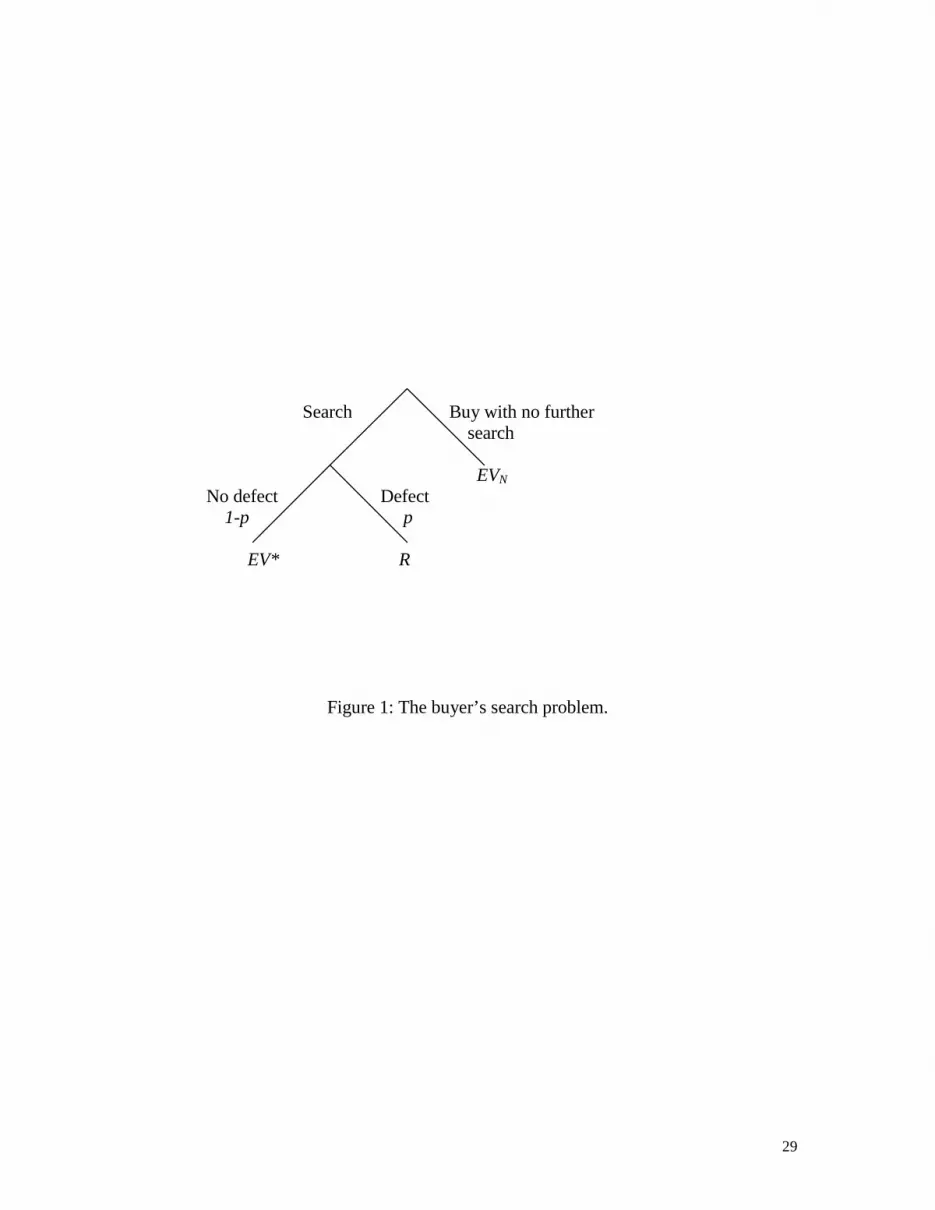
record. The problem is to determine when to stop searching. Figure 1 shows the

structure of the search problem at an arbitrary point t in the process, assuming that no

defect has been found in the previous t-1 records.

prior to improving a piece of land. For a related analysis, see Thomas Miceli and C.F. Sirmans, The Mistaken Improver Problem, 45 J. Urban Econ. 143 (1999). 8 Below, however, we let p be a function of the level of development in a given jurisdiction. 9 Clearly this abstracts from omissions in the record that could lead to future claims against the title. See, generally, C. Denton Bostick, Land Registration: An English Solution to an American Problem, 63 Indiana L. J. 55 (1987). We ignore this problem for simplicity, though it could easily be included without altering the basic results. In effect, it would represent a background risk that could not be eliminated by search. Insuring against this risk is the function of title insurance. See Cribbet, supra note 2, at 297. 10 See, e.g., Michael Rothschild, Models of Market Organization with Imperfect Information: A Survey, 81 J. Pol. Econ. 1283 (1973); and John Lippman and J. J. McCall, The Economics of Job Search: A Survey, 14 Econ. Inquiry 155 (1976).

5

Starting at the top of the tree, the searcher either searches one more record, which

yields an expected return of EVS(t-1), or he can stop and buy the parcel, which yields an

expected return of EVN(t-1). If he searches one more record, he finds a defect with

probability p and no defect with probability 1-p. If he finds a defect, then according to

(1) he should stop and invest in his next-best option, yielding R. If he finds no defect, he

continues optimally, which yields an expected return of EV*(t).

The preceding argument implies that search continues until one of three things

happens:11 (1) the searcher finds a defect; (2) the searcher inspects all T records; or (3)

the searcher stops searching at some t*<T. Our analysis will focus on when each of the

last two outcomes is the result of an optimal title search.

In order to characterize the optimal search process, we first need to derive an

expression for EVN(t). Recall that this is defined to be the expected value of the parcel

after t records have been examined, assuming that no defect has yet been found. This

expression is easily derived as follows. In period t=T-1, all but the last record have been

searched. The last search therefore reveals either a defect or that the title is clear. Thus,

(2) EVN(T-1) = pv + (1-p)V.

Now more forward to t=T-2. In this period, two records are left to be searched. Thus,

(3) EVN(T-2) = [p+p(1-p)]v + (1-p)2V ,

where the expression in the square brackets represents the probability that a defect is

found in either the next-to-last or last record, and (1-p)2 is the probability that no defect is

found in either of the last two periods.12 Generalizing, we have

11 This assumes that it is optimal to begin searching in the first place. We state the condition for this to be true below. 12 Note that the time until a defect is first found is therefore a random variable with a geometric probability distribution.

6

(4) VpvpptEV tTtT

N−

−−

=

−+−= � )1(])1([)(1

0τ

τ

Note that this expression is increasing (step-wise) in t. That is, EVN(t) becomes larger the

fewer records there are left to be searched , given that no defect has been found to date.

Further, EVN(T)=V; that is, if no defect has been found after searching the entire record,

the title is clear. Finally, we assume that

(5) VpvppEV TT

N )1(])1([)0(1

0−+−= �

−

=τ

τ ≥ R,

implying that the searcher prefers to purchase the parcel in question over his next-best

alternative even before he has begun searching the record.13 This reflects the notion that

most title search is triggered by an individual’s interest in purchasing a parcel of land.

Title search therefore potentially prevents the transaction from occurring.14

III. Optimal Search

Given the definition of EVN(t), we can now characterize optimal search for the

potential buyer. We first consider the case where it is optimal to search the entire record.

Suppose that the searcher, employing his optimal search strategy, has reached record

t=T-1 and has found no defects. The question is whether he should search the last record

or stop. His return from stopping is given by (2). In contrast, the expected value of

searching the last record is

(6) EVS(T-1) = pR + (1-p)V – c(T) ,

13 Note that EVN(0) approaches v as T approaches infinity. However, EVN(0) is strictly greater than v for finite T. Thus, (5) will hold for small enough T given V>R. 14 It is conceivable that a prospective buyer could search the title of a parcel that he would not buy initially (i.e., (5) does not hold) in hopes that he would discover no defects and eventually find the parcel desirable (i.e., EVN(t)>R for some t given that EVN(t) is increasing in t). This scenario seems less plausible and also presents some analytical difficulties without yielding significant insights, so we do not pursue it here.

7

which reveals the status of the title with certainty. Thus, if no defect is found, the buyer

purchases the parcel, but if a defect is found, he invests in his next-best option.

It is optimal to search the last record if EVS(T-1)>EVN(T-1), which yields the

condition

(7) pR + (1-p)V – c(T) ≥ pv + (1-p)V

or

(8) p(R-v) ≥ c(T).

The left-hand side represents the marginal benefit of one more search. It equals the

probability of finding a defect times the savings from investing in the next-best option

rather than buying the parcel with a defective title. Searching the last record is optimal

when this benefit exceeds the marginal cost of search.

The preceding is a special case of the general search rule under which t* < T is

the last record that the searcher inspects. Using the above definitions, the expected value

of searching record t*, given no defects in the previous t*-1 records, is

(9) EVS(t*-1) = pR + (1-p)EV*(t*) – c(t*),

where

(10) EV*(t*) ≡ max[EVS(t*), EVN(t*)]

is the expected value of continuing to search optimally thereafter. If instead the searcher

stops after inspecting t*-1 records, his return is simply EVN(t*-1). Since t* is the last

record searched (by definition), then

(11) EV*(t*) = EVN(t*).

Substituting this into (9), we obtain the conditions for t* to be the last record searched:15

15 We assume that when indifferent, the buyer searches.

8

(12) pR + (1-p)EVN(t*) – c(t*) ≥ EVN(t*-1)

and

(13) pR + (1-p)EVN(t*+1) – c(t*+1) < EVN(t*).

Using the definition of EVN(t) in (4), (12) simplifies to

(14) p(R-v) ≥ c(t*),

which has the same form and interpretation as (8). Repeating this process for (13) yields

(15) p(R-v) < c(t*+1).

Figure 2 illustrates this result. (In the graph, t is treated as a continuous variable

for simplicity.) Note that the marginal benefit of searching one more record is constant

over search time, given the time-invariance of the variables R, v, and p. However, the

marginal cost of search increases with the length of search for the reasons noted above.

Thus, search ends when the marginal cost equals the marginal benefit. It follows that

search commences in the first place if

(16) p(R-v) > c(1).

If (16) does not hold but (5) does, then the buyer purchases the parcel without inspecting

the record at all.

Comparative statics follow directly from (14) and (15) and are readily seen using

Figure 2. As the left-hand sides of (14) and (15) increase, the marginal benefit of

additional search increases, leading to an increase in the optimal length of search, t*.

Thus, records are searched further into the past as (i) p, the probability of a defect,

increases, (ii) R, the next-best option, increases, or (iii) v, the value of the parcel with a

defective title, decreases. Note that a decrease in v is equivalent to an increase in the cost

of a defect, k, holding V fixed (and recalling that k≡V-v). Therefore, the buyer will search

9

further back the costlier is a defect. Alternatively stated, the buyer will search back

further the larger is the expected value of the claim.

To this point, we have defined t to be the number of records searched, rather than

the number of years. Some jurisdictions, however, will have more entries or records per

year, due, for example, to greater rates of development. To allow for this, let n be the

number of title-related records per year in a given jurisdiction, which is viewed as a

parameter by individual searchers. If t* is the optimal number of records to search (as

derived above), then the optimal number of years to search, denoted y*, must satisfy t* =

ny*, or

(17) y* = t*/n.

It follows that jurisdictions with greater historic rates of land development (i.e., those

with higher n) should have shorter optimal search periods measured in years, ceteris

paribus.

Higher land development rates, however, might also generate an indirect

offsetting effect on the optimal search period. Specifically, higher development rates

create more opportunities for errors to enter the record.16 In this case, p would be an

increasing function of n in (14) and (15), making the numerator in (17), t*, a decreasing

function of n. This implies that a greater number of title related records per year, n, leads

to a longer optimal search period, y*, thereby offsetting the direct effect of n in

shortening the search period through the denominator of (17). The overall impact of

development is therefore ambiguous.

16 See Jeffrey Netter, P. Hersch, and W. Manson, An Economic Analysis of Adverse Possession, 6 Int’l Rev. Law & Econ. 217 (1986).

10

As an illustration of the preceding analysis, consider the following numerical

example. Let V=500, v=300, R=350, and p=.01. Given these values, the expected

marginal benefit of search is p(R-v)=5. If we let the cost function be given by

(18) 2)( tctc ⋅= ,

then we can use (14) and (15) to determine the optimal stopping time for different values

of the parameter c. The results are shown in Table 1. They show that the optimal search

time is decreasing in c. Table 1 also shows the value of EVN(0) for different values of T.

Note that condition (5) is satisfied for all T, implying that in this example, the expected

value of the parcel prior to search exceeds the buyer’s reservation price.

IV. Empirical Analysis

In this section we explore the empirical implications of the model using cross-

state data. Most states have guidelines, established by statute or less formally, dictating

how far back a title search should extend. For example, several states have enacted

Marketable Title Acts whose purpose is to limit title searches to a reasonable length.

They accomplish this by extinguishing most interests in land not recorded during the

statutorily specified period.17 (In this sense, they function like statutes of limitations.) In

states without statutes, local bars or title insurers often set search lengths. In these states,

prior interests are not eliminated by law, leaving the risk of loss on the purchaser, and

ultimately the title insurer.18 If anything, guidelines in these states should therefore be

more responsive to economic factors.

17 Excepted interests include mineral rights, easements, interests of persons in possession, and claims of the federal government. See Dukeminier and Krier, supra note 3, at 711, 717. 18 See Paul Goldstein, Real Estate Transactions, 266 (1980)

11

Several points bear emphasis in order to draw the connection between the

theoretical model and the empirical study. First, although we have characterized the

optimal search procedure from the buyer’s perspective, it is also the socially optimal

search procedure given that the buyer internalizes the value of any claim through k, the

cost of repairing the defect. In this sense, the optimal search length balances the value to

would-be purchasers of quieting title against the value of any third-party claims. Our

hypothesis is that state search guidelines embody this social trade-off.

Second, the typical potential buyer does not conduct the title search; most do not

have the expertise. This creates a potential principal-agent problem. The information and

skill asymmetry make it difficult for the buyer either to stipulate a search requirement or

verify that the search covers the agreed upon time period. A statutory search requirement

resolves both problems for the buyer. The presence of insurance further insulates buyers

from the need to worry about optimal search. As noted above, however, title insurers

have a strong interest in ensuring that search is optimal. They can do this by setting the

guidelines themselves in the absence of a statute, or by exerting political pressure on

legislatures to establish efficient guidelines.19

Finally, search requirements are state-wide, not transaction-specific. Clearly, the

optimal search length can vary across individual properties even within a single

jurisdiction. However, our data do not permit analysis below the state level. We do not

offer a formal model of search demand aggregation, but instead envision the search

requirement as reflecting the interplay of coincident and competing interests in the

19 We do not seek to model the process by which they exert this pressure, but instead conjecture that they have sufficient political influence that the statutes will tend to reflect their interests. We used a dummy variable to test whether search lengths set by statute differed from those set by non-statutory means and found no significant effect.

12

political process. Factors that lead to longer or shorter optimal search for individuals will

therefore likely lead to a longer or shorter aggregate search requirement to the extent that

the political process reflects social welfare.

A. Single Equation Model

We first consider a single equation model. The dependent variable is SEARCH,

which is defined to be the state’s established length of title search (measured in years).

Table 2 reports the lengths of title search for the states in our sample using data drawn

from Boackle.20

Some states have no set length but instead require that the entire title history of a

parcel of land be searched back to the state’s date of patent.21 In terms of the theory, this

represents a corner solution for which condition (8) holds. For these states, we define the

required length of search as the difference between 1990 and the date of patent.22 Other

states specify a range of possible search lengths, which vary by type of property or by

region; for example, the search length in Alabama varies from 40 to 60 years. For these

states, we use the average specified search length across property types or regions.

Boackle does not contain information on the search length in five states:

Colorado, Hawaii, Illinois, Indiana, and Tennessee. Through personal phone interviews

with industry employees, we were able to ascertain with reasonable accuracy the search

length in Colorado and Tennessee. In the three remaining states, however, there were

20 K. F. Boackle, Real Estate Closing Deskbook (1997). 21 These states are Alaska, Arizona, California, Florida, Idaho, Kansas, Montana, Nebraska, Nevada, North and South Dakota, Oregon, Texas, and Washington. 22 The United States acquired Alaska in 1867 in the Alaska purchase. Arizona, California, and Nevada were acquired in the Mexican cession of 1848. Florida was ceded from Spain in 1819. Idaho, Oregon, and Washington were acquired through the Oregon compromise in 1846. Kansas, Montana, Nebraska, North

13

rather wide differences of opinion as to what exactly constituted a legally reasonable

search. When asked what they felt a reasonable search to be, industry employees gave a

range of answers. For example, some gave standards measured in years, while others

said that a reasonable search went back three previous owners, or even that a reasonable

search varied with market conditions and type of property. Of course, a search covering

the whole record (back to patent) would certainly meet any standard in these states, but it

would not reflect the outcome of a cost-benefit calculation. For these reasons, we

exclude these three states from the analysis as possessing indeterminate search lengths.

As for the independent variables, the theoretical model identifies several key

determinants of optimal search length: the probability of an error occurring in the title

record (p), the costs of repairing an error in title (i.e., the value of protecting the

claimant’s rights) (k), the cost of searching titles (c), and the number of titles that need to

be searched per year (n). We construct empirical proxies to capture the effects of each of

these factors on the title search period. Table 3 reports summary statistics for all of the

variables used in the single equation model.

The variable RISK is included as an explanatory variable in the SEARCH equation

to capture the expected cost of a defect, which equals the probability of an error occurring

in the title record times the cost of repairing the defect. This variable is defined as the

sum of the owners’ and lenders’ premiums for title insurance for a $50,000 parcel of land

and is calculated from the title insurance rates reported by Boackle.23 The rationale for

using this variable is the fact that the title insurance premium should reflect the market

Dakota, and South Dakota were all acquired in the Louisiana Purchase of 1803. The U.S. acquired Texas in 1845. 23 Boackle, supra note 20. Two states, Iowa and Missouri, do not have information on title insurance rates, so these states are not included in the data set.

14

pricing of the risk of a defect. To the extent that higher title insurance rates reflect greater

risk of title errors (i.e., higher p), and/or a greater cost of repairing a defect (i.e., higher

k), they should lead to a longer search duration. We therefore expect to find a positive

coefficient on RISK in the SEARCH equation.

We include each state’s developed land as a percentage of total land in the search

equation as an additional measure of the likelihood of error. The variable

%DEVELOPED is defined as the percentage of nonfederal acres in a state that are

developed and was obtained from the 1990 Census. The requisite information for

calculating this variable is not available for Alaska, so we exclude Alaska from the data

set.

As noted above, higher development rates lead to more frequent property transfers

and thus to a greater likelihood of errors.24 Commercial real estate transactions in

particular are generally more complicated than other types of land sales, especially

agricultural land sales, which may amplify the probability of errors. Further, there are

more likely to be easements on property in developed areas, rendering title records more

vulnerable to important omissions. Finally, the Comprehensive Environmental Response,

Compensation, and Liability Act of 1980 (CERCLA) greatly increased the liability of

property owners for damages and cleanup costs due to hazardous waste. As Boackle

notes "Virtually every transaction involving commercial property…will prompt the

question of hazardous waste."25 Thus, higher rates of development in a state may lead to

greater risks due to the increased possibility of hazardous waste contamination. Based on

these factors, we anticipate a positive coefficient on this variable.

24 Netter, Hersch, and Manson, supra note 16. 25 Boackle, supra note 20, at 80.

15

The variable TITLECOSTS is included in the SEARCH equation as a measure of

the costs of conducting a title search. A 1980 RESPA publication contains results of a

HUD survey of state-by-state closing costs in 1979.26 This publication reports average

title charges by state, which include the costs of conducting a title search. Comparable

data were not available for 1990, so we included these numbers as the best measure for

the costs of title search. The optimal title search model predicts that these costs will have

a negative effect on SEARCH.

The final variable in the SEARCH equation is TURNOVER, which is an index

measuring the total number of titles that must be searched per year for an average

property. We include this variable to capture the role of n in the theoretical search model.

Basically, the TURNOVER variable is an estimate of the average number of times a house

existing in 1990 has changed hands over the previous forty years. This variable is

constructed as follows.

Our calculation takes into account both the variation in the age distribution of

houses, and variation in the turnover rate. For each state, we employ U. S. Census data

on the historical evolution of the owner-occupied housing stock and data on recent

movers as a percentage of the population in the state. To begin, we obtain data on recent

movers back to 1960. We use the percentage of recent movers at the end of each decade

as an estimate of the average rate of turnover during the decade. For example, if 10% of

homeowners in a particular state were identified as recent movers in the 1970 census,

then we infer that about 10% of the 1970 housing stock changed hands during the year.

Assuming that the percentage of recent movers at the end of the decade is reasonably

close to the percentage of recent movers throughout the decade, then the average house

26 RESPA, Real Estate Closing Costs (1980).

16

changed hands approximately once during the decade, given that 10% of houses on

average changed hands during any year.

To transform the recent mover information into a measure of average turnover,

we need to control for the age distribution of the housing stock. The housing stock in

1960, 1970, 1980, and 1990 is readily available in the census. We measure the extent to

which the existing housing stock changed hands in each of the decades 1960, 1970, and

1980 using the age distribution of houses existing in each decade and the number of

recent movers. Our measure of turnover is computed as:

)}()()({10890

6060

90

7070

90

808090 S

SREMOVESSREMOVE

SSREMOVEREMOVETURNOVER ++⋅+⋅=

where REMOVE is the percentage of households that are identified as recent movers, and

tS is the number of owner-occupied housing units existing in 1990 that were also part of

the housing stock in decade t. (We weight REMOVE90 by 8 instead of 10 to take into

account that the 1990 census defined recent movers differently than did previous

censuses. Prior to 1990, the census defines recent movers as those who moved into their

houses within the previous twelve months; the 1990 census, on the other hand, defines

recent movers as those who moved within the previous fifteen months.) The constructed

measure ranges in value from a maximum of 4.96 for Wyoming to a minimum of 2.35 in

Massachusetts, with a mean value of 3.24.

The predicted effect of TURNOVER on the optimal search length is ambiguous

given the offsetting effects of n. On the one hand, a greater TURNOVER indicates that

more records must be searched per year, which tends to shorten the optimal search

duration. On the other hand, greater TURNOVER reflects a greater volume of market

17

activity for a given stock of housing. As described above, this implies that errors in the

title record are more likely, which tends to increase the search length in the theoretical

model.

We estimate the following SEARCH equation using ordinary least squares:

(19) εββ

βββ+++

++=)(%)(

)()()(

54

210

DEVELOPEDLogTURNOVERLogCOSTTITLELogRISKLogSEARCHLog

The estimates are presented as model I in Table 5.

The empirical model fits the data fairly well (the adjusted R2=.48), and the

estimated parameters have the expected signs. The RISK variable is positive and

significant at the 1% level, indicating that states with higher risks of title defects (as

reflected by the title insurance premium) also have longer search periods. The

TURNOVER coefficient is positive and significant at the 1% level, and %DEVELOPED

is significant at the 10% level. Both of these results are consistent with our theoretical

argument that states with higher levels of development have longer search lengths

because of the greater likelihood of a title defect. Finally, the coefficient on the

TITLECOST variable is negative and significant at the 5% level, reflecting the expected

negative impact of search costs on the length of search.

B. Simultaneous Equations Model

Although the single equation model performed well, there are two problems

associated with our use of RISK as an explanatory variable. The first is the possibility that

RISK is endogenously determined with the dependent variable in the SEARCH equation.

In particular, title risk may be lower in states with longer search lengths because more

18

records must be searched. As a result, the insurance premium would be lower. In this

section we use a simultaneous equation system to address this problem.

A second potential problem with the RISK variable is that the costs of title search

are included in the insurance premium in some states, while in others the premium

includes only the cost of indemnifying against title risk. This difference in industry

practice has its roots in the different organizational structures of the title search and title

insurance industries in different states. Specifically, the Special Committee on Lawyers’

Guaranty Funds states that “…where title insurance companies gain control over title

evidence, by acquiring the abstract companies and maintaining the abstracting function in

their own plants for their own use, their rate system is changed to one that includes title

information procurement and examination along with the ‘pure insurance’ in a single

charge.”27 In states in which some components of search costs are included in the

premium, title insurance companies generally maintain their own title plants.

While it is at least conceptually feasible to purge the impact of search costs from

the RISK variable and come up with a set of estimated “pure insurance” rates for each

state, information may be lost due to the difference in organizational form in states in

which the search costs are included in the premium. For example, when title insurance

companies maintain their own title plants, they may take greater care in maintaining

records because they have a vested interest in the records. Title insurance companies

may also find it easier and cheaper to search their own title plants. The other variables

included in the search equation are meant to capture both the effects of the likelihood of

error as well as title search costs, so we are confident that those variables, at least, are

27 Special Committee on Lawyers’ Title Guaranty Funds, The Concept, Organization, and Operation of Bar-Related title Assuring Organizations, ABA (1968), at 36-37.

19

picking up their intended effects. Nonetheless, the specification of the RISK equation in

our simultaneous system must take into account those factors influencing the variable

RISK.

The RISK equation is specified as follows:

(20) PRESEARCHNARROWACTCOSTINCPRICECOMP

MARKETSHRLogDEVELOPEDLogTURNOVERLogSEARCHLogRISKLog

8765

43

210

)()(%)()()(

δδδδδδ

δδδ

++++++

++=

The first variable on the right-hand side is SEARCH, the length of the title search. As

noted, this variable is included in the RISK model to control for the possibility that

SEARCH directly influences title risk. The second and third variables are TURNOVER

and %DEVELOPED. These two variables are included to control for the possibility that

these variables may influence the risk premium directly through the effects discussed

above. TITLECOST is omitted from equation (20) to identify the model. This reflects our

judgment that the cost of performing a title search should not directly influence the risk

of discovering a defect.

The remaining five variables in equation (20), MARKETSHR, PRICECOMP,

COSTINC, NARROWACT, and PRESEARCH, serve as instruments in the simultaneous

equation model. These variables capture institutional, technological, and business factors

that may influence the risk premium independently of the impact of title search. The two

variables, MARKETSHR and PRICECOMP, are included to capture the effects of the title

industry market structure in each state. These variables are drawn from information

reported by Quiner.28 MARKETSHR is defined as the percentage of insurance policies

written by the three largest firms in the state in 1973. Based on the survivor principle, this

28 S. Quiner, Title Insurance and the Title Insurance Industry, 22 Drake L. R. 711 (1973).

20

variable is included in the model to measure the potential economies-of-scale effects in

the industry. To the extent that scale economies exist, we expect a negative coefficient on

this variable.

The variable PRICECOMP is a dummy variable reflecting some interesting

results of a survey done by Quiner,29 in which people employed in the title insurance

industry were asked to assess the degree of price competition in their home state.

PRICECOMP equals zero if the response was “price competition nonexistent” in the

state, and one otherwise. We anticipate a negative coefficient on PRICECOMP,

indicating that greater perceived price competition is reflected in lower title insurance

premia.

While the data on the title insurance industry are old, there is little available

recent state level information about these aspects of the title insurance industry.30 Barring

radical changes in the title industry structure over the intervening years, however, these

variables should be adequate proxies for the intended measures. Since these market

variables were not available for all states, the sample size for the simultaneous equation

model is reduced to 35.31

The remaining variables in the RISK equation are included in order to capture any

effects of the legal or regulatory institutions of the state on the title insurance industry.32

COSTINC is a dummy that equals one if title insurance companies in the state are

allowed to include the costs of their title search directly in the insurance premium.

29 Id. 30 These numbers have also been used recently by D. Barlow Burke, Jr., The Law of Title Insurance (1986), in discussing the nature of the title insurance industry. 31 The states included in the analysis were Alabama, Arkansas, California, Connecticut, Delaware, Florida, Idaho, Kansas, Kentucky, Louisiana, Maine, Maryland, Michigan, Minnesota, Nebraska, New Hampshire, New Jersey, North Carolina, North Dakota, Ohio, Oklahoma, Oregon, Pennsylvania, Rhode Island, South Carolina, South Dakota, Texas, Utah, Virginia, Washington, West Virginia, Wisconsin, and Wyoming.

21

NARROWACT is a dummy that equals one for those states that most narrowly define and

restrict the duties and activities of title insurers and zero otherwise. Finally,

PRESEARCH is a dummy variable that is included to control for another feature of the

state regulatory or institutional environment; specifically, whether or not a state requires

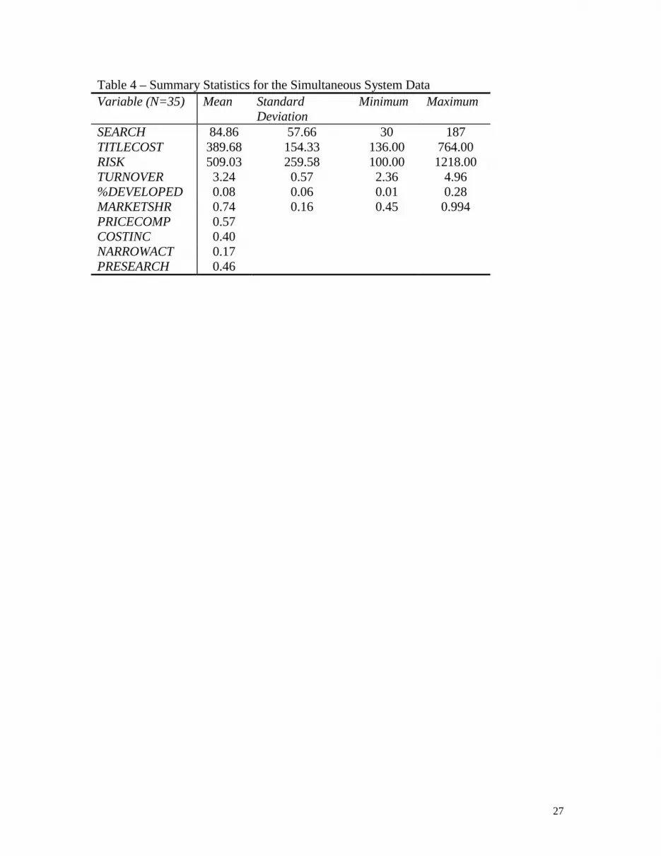
that a title search be completed before an insurance policy can be issued. Summary

statistics for the variables used in the simultaneous equations model are presented in

Table 4.

We first estimate equation (20) by ordinary least squares, dropping the variable

Log(SEARCH). The results are presented as model II in Table 5. This equation verifies

that increases in turnover of the housing stock, or increases in the development rate, do

indeed increase the risk to title as measured by the variable RISK. Also, RISK is smaller

in states in which pricing was judged to be relatively competitive, evidenced by the

negative sign of the coefficient on PRICECOMP. There is also evidence of scale effects

in the title insurance industry since those states in which a large percentage of the policies

are written by a few firms (a high value for MARKETSHR) charge lower rates. Finally,

the positive coefficient on COSTINC reveals that including search costs in the premium

generally raise the gross title insurance premium, as expected.

Model III includes the variable SEARCH in the RISK equation, and estimates the

two equations simultaneously using iterated two-stage least squares. The SEARCH

equation appears very similar to its single-equation counterpart, both in terms of the

magnitudes and signs of the coefficients, and also the significance levels. This suggests

that the OLS results were not unduely affected by the simultaneity bias from the variable

RISK. The insignificant coefficient on SEARCH in the RISK equation reinforces this

32 These variables were obtained from D. Barlow Burke, Jr., The Law of Title Insurance (1991).

22

point—that is, the required search duration does not appear to affect the title insurance

premium in a significant way. The other coefficients in the RISK equation also reveal the

same relationships found for the version of the equation estimated using ordinary least

squares.

Models IV, V, and VI further test the robustness of the results. Model IV drops

SEARCH from the RISK equation, and uses the predicted values of RISK from the first

stage estimates of that equation when estimating the SEARCH equation. The SEARCH

equation estimates are again similar to those in the single equation model.

Models V and VI apply a time-duration methodology to the data, treating the

dependent variable SEARCH as the time at which a specified event occurs. In this case,

the event is “stop title search.” The states in which search goes back to patent are treated

as right-censored observations where the event “stop the title search” never actually

occurs. Model V estimates the search equation alone, while Model VI uses predicted

values of RISK, obtained from model IV.33 The coefficient estimates generated by this

methodology are again very similar to those obtained for the other specifications. The

consistency of the estimates in the search equation across the various models provides

strong evidence that state guidelines for title search are influenced by the economic

factors identified in the title search model.

V. Conclusion

When ownership of land or any asset is uncertain, would-be buyers have to decide

how much effort to devote to learning whether or not the seller is the rightful owner. In

doing so, they balance the gains of increased certainty against the costs of searching

23

further back in the public title records. In this paper, we examined the factors

determining the optimal duration of title search. The theory predicted that a buyer should

continue searching sequentially as long as the benefit from searching one more record

exceeds the cost, where the benefit consists of the expected gain from avoiding purchase

of a parcel with a defective title. In general, optimal search does not prescribe that buyers

should search all available records, which in turn implies that some residual title

uncertainty remains.

The comparative statics from the model yielded several factors that affect the

optimal length of search. We used cross-section data on state guidelines for title search to

test the extent to which these guidelines are influenced by the economic factors identified

in the optimal search model. The estimates were consistent with the predictions of the

theory across a variety of specifications of the empirical model. The results therefore

support the notion that state title search guidelines reflect an effort to balance the

marginal benefits and costs of title search in property transfers.

33 Models V and VI were both fitted assuming that search time is log-normally distributed.

24

Table 1: Numerical Example. c t* T EVN(0)

.05 10 10 480.88

.025 14 20 463.58

.01 22 30 447.94

.005 31 40 433.79

.0025 44 50 421.00

.001 70 60 409.43 70 398.97 80 389.50 90 380.95 100 373.21 V=500, v=300, R=350, p=.01

25

Table 2: Search length.

State Search Length State Search Length Alabamaa 50 Nevadab 142 Alaskab 123 New Hampshire 35 Arizonab 142 New Jersey 60 Arkansas 40 New Mexico 30 Californiab 142 New York 40 Coloradoc 187 North Carolinaa,d 35 Connecticutd 40 North Dakotab 187 Delaware 60 Ohiod 60 Floridab,d 171 Oklahomad 30 Georgia 50 Oregonb 144 Idahob 144 Pennsylvania 60 Iowad 40 Rhode Island 50 Kansasb 187 South Carolinad 40 Kentuckya 50 South Dakotab 187 Louisiana 65 Tennesseec 30 Maine 40 Texasb 145 Maryland 60 Utah 40 Massachusettsd 50 Vermontd 40 Michigand 40 Virginia 60 Minnesotad 40 Washingtonb 144 Mississippid 75 West Virginia 60 Missouri 45 Wisconsind 60 Montanab 187 Wyomingb 187 Nebraskab 187 Source: K. Boackle, Real Estate Closing Deskbook (1997), various pages, and personal interviews (see note c below). aAverage over a range. bSearch back to patent. cObtained from personal interviews. dSet by statute.

26

Table 3 – Summary Statistics for the Single Equation Model Data Variable (N=42) Mean Standard

Deviation Minimum Maximum

SEARCH 87.05 57.24 30 187 TITLECOST 388.60 143.48 136.00 764.00 RISK 500.95 254.10 100.00 1218.00 TURNOVER 3.26 0.59 2.35 4.96 %DEVELOPED 0.07 0.06 0.01 0.28

27

Table 4 – Summary Statistics for the Simultaneous System Data Variable (N=35) Mean Standard

Deviation Minimum Maximum

SEARCH 84.86 57.66 30 187 TITLECOST 389.68 154.33 136.00 764.00 RISK 509.03 259.58 100.00 1218.00 TURNOVER 3.24 0.57 2.36 4.96 %DEVELOPED 0.08 0.06 0.01 0.28 MARKETSHR 0.74 0.16 0.45 0.994 PRICECOMP 0.57 COSTINC 0.40 NARROWACT 0.17 PRESEARCH 0.46

28

Table 5 – Estimated Models I II III IV V VI Estimation OLS OLS Iterated 2SLS Iterated 2SLS Right-Censored Right-Censored (2SLS) N=44 N=37 N=35 N=35 N=44 N=35 Dep. variable = Log(SEARCH)

Independent Variables

Coefficient t-stat. Coefficient t-stat. Coefficient t-stat. Coefficient t-stat. Coefficient t-stat. Coefficient t-stat.

CONSTANT 3.39** 2.23 4.48** 2.57 4.48** 2.57 2.72 1.23 3.47 1.36 Log(RISK) 0.47* 2.76 0.47*** 1.96 0.47*** 1.96 0.65* 2.68 0.56** 1.81 Log(TITLECOST) -0.63** -2.50 -0.76** -2.43 -0.76** -2.43 -0.85** -2.26 -0.738** -1.90 Log(TURNOVER) 2.20* 3.50 2.20* 3.19 2.20* 3.19 3.40* 3.64 3.103* 3.13 Log(%Developed) 0.31*** 1.86 0.41** 2.14 0.41** 2.14 0.43** 1.86 0.428** 1.76 R2 0.53 .50 0.50 - - Adjusted R2 0.48 .43 0.43 - - Dep. variable = Log(RISK)

Independent Variables

CONSTANT 4.89* 12.73 5.648* 5.70 4.84* 11.73 4.839* 11.73 Log(SEARCH) - -0.409 -1.02 - - Log(TURNOVER) 1.05** 2.71 1.999*** 1.80 1.03** 2.54 1.030** 2.54 Log(%Developed) 0.12 1.38 0.148 1.07 0.09 1.04 0.090 1.04 Log(MARKETSHR) -0.76*** -3.17 -0.735*** -1.96 -0.81* -3.19 -0.809* -3.19 PRICECOMP -0.20*** -2.03 -0.339*** -1.92 -0.25** -2.35 -0.246** -2.35 COSTINCLUDE 0.67* 6.08 0.674* 3.72 0.62* 5.18 0.615* 5.18 NARROWACT -0.36** -2.68 -0.325 -1.61 -0.37** -2.75 -0.373** -2.75 PRESEARCH 0.005 0.05 0.080 0.51 0.05 0.42 0.045 0.42 R2 .78 .57 0.79 0.7886 Adjusted R2 .73 .44 0.73 0.7337 * denotes significance at the 1% level ** denotes significance at the 5% level *** denotes significance at the 10% level

29

Search Buy with no further search EVN No defect Defect 1-p p EV* R

Figure 1: The buyer’s search problem.

30

$ c(t)

p(R-v) t* t

Figure 2: The optimal stopping time.