Embed Size (px)
Citation preview
156
REVISTA INVESTIGACIÓN OPERACIONAL Vol. 30, No.2, 156-172, 2009
ESTIMATING THE DIFFERENCE OF MEANS
WITH IMPUTATION OF THE MISSING
OBSERVATIONS Carlos N. Bouza Herrera*1 and Dante Covarrubias Melgar** *Facultad de Matemática y Computación de la Universidad de La Habana, Cuba ** Universidad Autónoma de Guerrero
ABSTRACT We consider the use of a finite population model for estimating the difference of the means of two variables under a mechanism for missing observations. The information available on the two variables is used for imputing the corresponding missing data. The proposed estimator is characterized by means of the expected squared error. Data from an environmental study are used for illustrating the performance of the estimator.
KEY WORDS: unbiasedness, mean squared error, variance, approximated moments
MSC: 62D05
RESUMEN Consideramos el uso de un modelo de población finita para estimar la diferencia de dos medias bajo un mecanismo de observaciones perdidas. La información existente sobre las dos variables es usada para imputar los datos faltantes correspondientes. El estimador propuesto es caracterizado por medio del error cuadrático medido esperado. Datos provenientes de un estudio medio ambiental son usados para ilustrar el comportamiento del estimador.
1. INTRODUCTION The use of imputation techniques for dealing with missing information is a theme of actuality. See for example Chang et al. (2000), Chang- Huang (2001), Liu et.al. (2004), Rueda and González (2004), Rueda et al. (2006a and 2006b), Tsukerman (2004), Zhou et.al. (2001). Applications frequently pose to the surveyor the need of estimating a difference. The aims of the inquiry are to measure the same variable twice in the sampled units or two different variables are measured in them. We use the finite population framework as the theoretical frame for estimating the difference,Δ, between the means of two variables X and Y. Lin (1971) considered the existence of missing observations under the normality of the variables. Bouza (1983) considered the finite population case and derived an estimator of the difference of means, dropping the normality assumption and considering that the missing observations should be considered as non responses.
157
The main objective of this paper is to develop an estimator of the difference of means using the imputation proposed by Zhou et al.(2001). Section 2 presents the problematic of estimating the difference of two parameters and discusses the particularities of the difference of means. Section 3 is concerned with the missing observation problem and the proposal of Zou et al. (2001). The estimator proposed by Bouza (1993) is considered under the missing observation model. Its bias is deduced and a bias corrected one is proposed. The mean squared error is developed; Section 4 is proposed to use a Jacknife procedure for estimating it. Data from environmental studies are used for illustrating the behavior of the proposals by computing the percent of samples in which the true parameter is covered by the confidence intervals computed; 2. ESTIMATION OF A DIFFERENCE
Applications frequently pose to the surveyor the need of estimating a difference. The aims of the inquiry are to measure the same variable twice in the sampled units or two different variables are measured in them. Some current examples of the need of estimating a difference in contemporary research are given below.
An example in bioinformatics is the estimation of evolutionary distances between biological sequences they are the variables needed for phylogenetic tree inference, which provides the dataset for developing comparative genomics analyses. Always the measurement is made over large sets of genes or proteins etc. The use of maximum likelihood needs of expensive computation as the datasets are commonly very large. Dessimoz et.al. (2006) assumed the normality of the distance between homologs and the evaluation of them allow to estimate the difference of the distances in a triplet. Similar problems are posed in different papers where the estimation of a difference is present see the research of Guo et.al. (2006) as an example.
Environmental studies need to obtain accurate measurement of different indexes. An important contemporaneous problem is described by the estimation of forest cover for effective management. The parameter of interest is the so called Normalised Difference Vegetation Index. It is based on the computation of the difference in the same sites using information provided by satellite photos. Similarly the difference between the air and sea temperature, and other bioclimatic variables are measured in the same sites twice and the individual differences are computed. See for example Ghosh-Mukhopadhyay (1980), Owe-Urso (2002), Xiao et.al. (2003), Singh et.al. (2005),
In sociology , psychology and other soft sciences the determination of differences between groups is a common task. For example the estimation of the so called consumer difference, achievements in education and other similar problems are based on the observation of the behavior of individuals under two situations or of matched pairs . That is the common case in the study of student response and in general in the evaluation of behavioral differences when a certain treatment is applied to a set of persons in the before-after scheme or by using matched pairs. See the papers of Klemz (1999), Kulik et.al. (1998), Germain-Scandura. (2005).
158
In Agriculture we can mention the need of establishing the effect of two politics, to estimate the growth of vegetables or the increase in the weigh of animals, the production of milk, meat etc. Actually the prediction of the production using remote sensing poses the same problem: to select sites and to measure them twice for estimating the increases. For example Xiao,(2003) needed to compute the estimated difference derived by two methods of cropland estimation as well as Cacace et.al. (2002) for evaluating storage policies..
The need of estimating differences is present in the study of voting in elections, of consumer attitudes and in many other opinion polls. Economical problems derive the need of estimating a difference as in audit, where the estimation of the difference of the results obtained in two audits is a common problem, see Wurst,et.al. (1991).
Medical research commonly use the estimation of a difference for evaluating the effect of a new treatment based on the individual differences computing results. The evaluation of blood pressure medicament control will be based on its measurement in the same patient before and after taking it. The same is valid for using a certain treatment. A similar analysis is present when testing the reliability of two electrocardiograms systems etc. Commonly a procedure generates the standard values (provided by a classic system or gold standard) and a new one generates alternative results in each individual in the study. The use of matched pairs is also frequent in these experiments. The interested reader can see how the estimation of a difference is present in medical papers as Silverman et.al. (1982), Stevenson-Ward (2003), Martinelli et.al. (2004).
Different statistical papers have considered the estimation of a difference
Δθ= θ(X)- θ(Y)
The variables of interest are X and Y and the parameters θ(X) and θ(Y) are defined by the particular problem. The robustness of the estimation of the difference of location parameters under censoring has been studied by Basak (1993). More papers have been written considering that θ(Z)=μZ, Z=X, Y. That is when we deal with the difference of means
Δμ= μX -μY
Different models for estimating the difference of means have been considered in the literature. Trybula (1991) considered this problem under an infinite population model. Alvo-Cabilio(1982), Hayre (1983), Chaturvedi (1986), Chou et.al. (1986), Mukhopadhyay-Darmanto (1988) and Mukhopadhyay-Sumitra (1994) considered the use of a sequential procedures under distributional hypothesis . Kelley (1977) combined sequential and Bayesian criteria for deriving a method for estimating the difference of means. A pure Bayesian approach was used by Rekab (1992) in the study of failure. Alvo-Cabilio (1989) assumed normality of the two variables and different sampling models were considered.
It is surprising that the estimation of the difference for other parameters has not received so much attention by the statisticians.

159
We will consider the use of a finite population model. The theoretical frame for estimating the difference can be described by considering a finite population U={1,…,N}. Defining a sampling design p(s), a convenient estimator should be derived Δ*θ and its statistical properties are deduced. The sampling error (Mean Squared Error)
MSM(Δ*θ)=E(Δ*θ- Δ*θ)2
Is derived for measuring the accuracy of the estimator. The practical problem is completely solved once we obtain an adequate estimator of MSM(Δ*θ). If Δ*θ is unbiased MSM(Δ*θ)=V(Δ*θ), where ‘V’ stands for variance. Then the different particular problems can be model accordingly. In this paper we will consider the case in which
Y,XZ,N
Z)Z(
N
1ii
Z ===∑=μθ
and p(s) is simple random sampling with replacement (srswr). Therefore if n is the sample size we measure (X, Y) in every sampling unit and a naïve estimator of Δ=μX -μY is
y,xzn
zz,y-xd
n
1ii
===∑=
Its unbiasedness follows form the fact that the sample mean is unbiased for the population mean and
n2
nn)y,x(2Cov)y(V)x(V)d(ECM xy
2y
2x σσσ
−+=−+=
Where ‘Cov’ is the covariance operator.
As stated in the introduction our interest is to derive an estimator of the difference of means when observations are missing.
4. MISSING OBSERVATIONS
4.1 The missing observation and the non response model (MONR)
Lin (1971) considered the existence of missing observations when estimating the difference of means. He considered that the sample s was partitioned in three mutually disjoint sub samples
.s(1)={i∈s⏐ (X,Y) are measured}
.s(2)={i∈s⏐ only Y is measured}
.s(3)={i∈s⏐ X) is measured}
160
Therefore we can compute only
2,1j,si,n
yy
3,1j,si,n
xx
jj
n
1iij
j
jj
n
1iij
j
j
j
=∈=
=∈=
∑
∑
=
=
His proposal was to use as estimator
2131P y)2(by)1(bx)3(ax)1(ad −−+=
The weights were determined looking for minimizing the variance, using the fact that the joint distribution of X and Y was a bivariate normal. The missing observations were generated by a random missing mechanism (RMM). To measure both variables was considered too expensive. A random experiment determined which sampled units were assigned to each sub sample.
Bouza (1983) considered the finite population case and derived an estimator of the difference of means, dropping the normality assumption and considering that the missing observations should be considered as non responses. That is, there was a refusal to give the information at the first visit. A second visit allowed obtaining responses from a subsample among the non respondents. The derived estimator was considered under three subsampling rules following the proposals developed in Bouza (1981). It is
n)'yx(n
n)y'x(n
n)yx(nˆ 333222111 −
+−
+−
==Δ NRdμ
Where the mean of X (Y) in s(3) (s(2)) is obtained by resampling.
We will reconsider the proposal of Lin (1971) under the finite population model but considering that there is a need of providing information on both variables in each sampled unit. Some of the examples given in the previous section illustrate this need. We will consider some cases. For example the bio-informatician needs to have an idea of the difference of the distances in each triple for obtaining the whole tree; to give estimates by region of the Normalized Difference Vegetation Index, or the difference in the cropland in each site, is expected by the agency; to develop analysis of groups of students or patients is expected, hence the sociologist or the physician need to have an idea of difference of the response of each individual. Then we may consider that though observations may be missing and an estimation of the difference can be made, we need to have an approximate measurement of the two variables in each selected unit. Hence it is not sufficient to use the approach of Lin (1971). The solution is to make imputations on the missing observations.
4.2 The RMM model
161
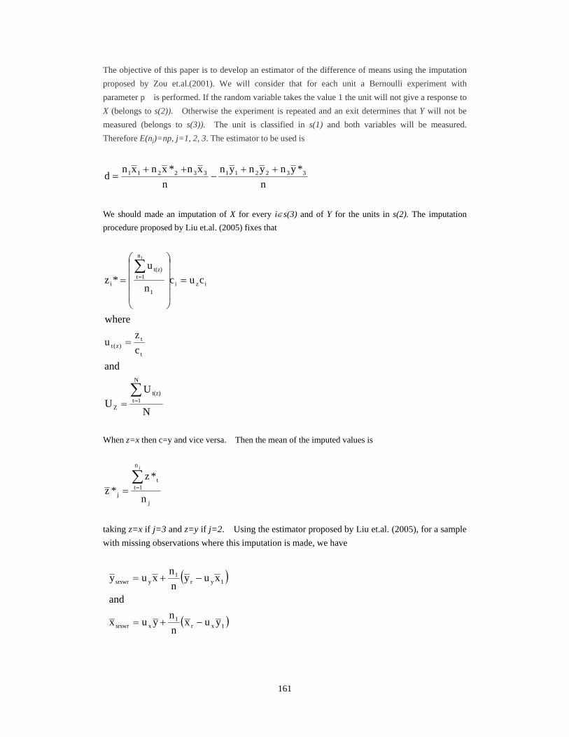
The objective of this paper is to develop an estimator of the difference of means using the imputation proposed by Zou et.al.(2001). We will consider that for each unit a Bernoulli experiment with parameter p is performed. If the random variable takes the value 1 the unit will not give a response to X (belongs to s(2)). Otherwise the experiment is repeated and an exit determines that Y will not be measured (belongs to s(3)). The unit is classified in s(1) and both variables will be measured. Therefore E(nj)=np, j=1, 2, 3. The estimator to be used is
n*ynynyn
nxn*xnxn
d 332211332211 ++−
++=
We should made an imputation of X for every i∈s(3) and of Y for the units in s(2). The imputation procedure proposed by Liu et.al. (2005) fixes that
N
UU
andcz
u
where
cucn
u*z
N
1tt(z)
Z
t
t)z(t
izi1
n
1tt(z)
i
1
∑
∑
=
=
=
=
=⎟⎟⎟⎟
⎠
⎞
⎜⎜⎜⎜
⎝
⎛
=
When z=x then c=y and vice versa. Then the mean of the imputed values is
j
n
1tt
j n
*z*z
j
∑==
taking z=x if j=3 and z=y if j=2. Using the estimator proposed by Liu et.al. (2005), for a sample with missing observations where this imputation is made, we have
( )
( )1xr1
xsrswr
1yr1
ysrswr
yuxnn
yux
and
xuynn
xuy
−+=
−+=
162
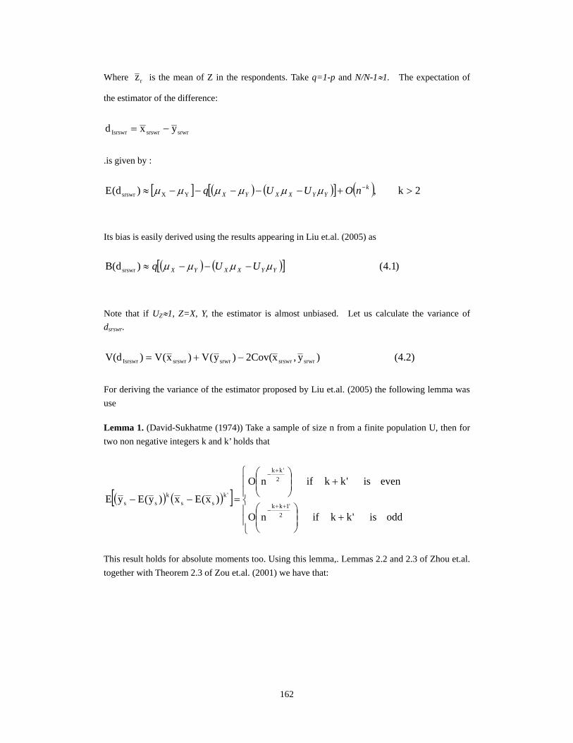
Where rz is the mean of Z in the respondents. Take q=1-p and N/N-1≈1. The expectation of
the estimator of the difference:
srwrsrswrIsrswr yxd −=
.is given by :
[ ] ( ) ( )[ ] ( ) 2k,)d(E YXsrswr >+−−−−−≈ −kYYXXYX nOUUq μμμμμμ
Its bias is easily derived using the results appearing in Liu et.al. (2005) as
( ) ( )[ ] )1.4()d(B srswr YYXXYX UUq μμμμ −−−≈
Note that if UZ≈1, Z=X, Y, the estimator is almost unbiased. Let us calculate the variance of dsrswr.
(4.2))y,x2Cov()y(V)x(V)V(d srwrsrswrsrwrsrswrIsrswr −+=
For deriving the variance of the estimator proposed by Liu et.al. (2005) the following lemma was use
Lemma 1. (David-Sukhatme (1974)) Take a sample of size n from a finite population U, then for two non negative integers k and k’ holds that
( ) ( )[ ]⎪⎪
⎩
⎪⎪
⎨
⎧
+⎟⎟⎠
⎞⎜⎜⎝
⎛
+⎟⎟⎠
⎞⎜⎜⎝
⎛
=−−++
−
+−
oddis'kkifnO
evenis'kkifnO
)x(Ex)y(EyE2
'1kk
2'kk
'kss
kss
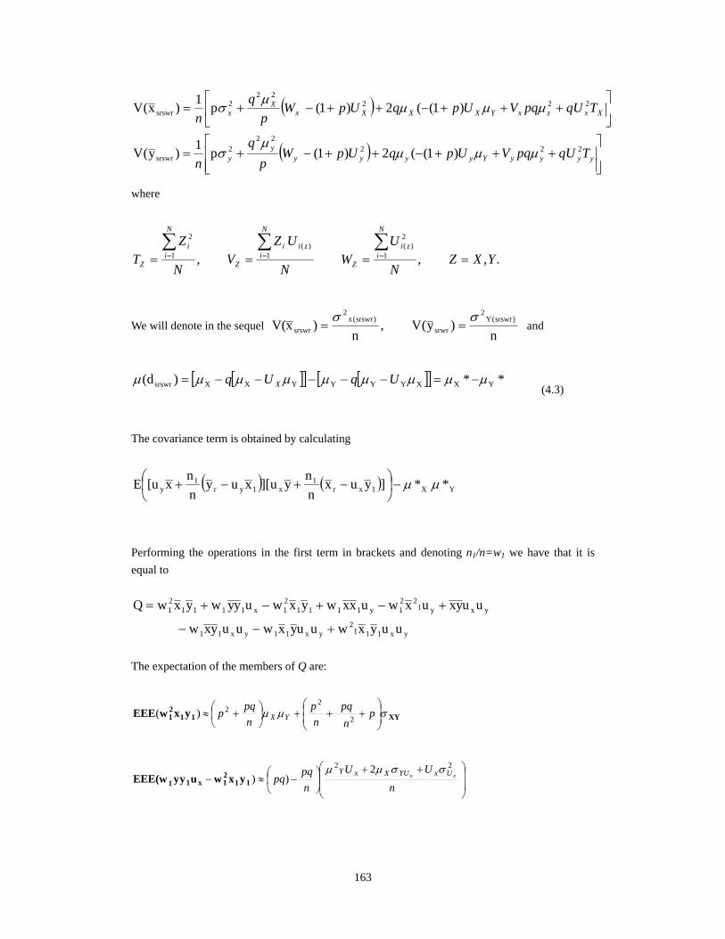
This result holds for absolute moments too. Using this lemma,. Lemmas 2.2 and 2.3 of Zhou et.al. together with Theorem 2.3 of Zou et.al. (2001) we have that:
163
( )
( )⎥⎥⎦
⎤
⎢⎢⎣
⎡+++−++−+=
⎥⎦
⎤⎢⎣
⎡+++−++−+=
yyyyYyyyyy
y
XxzxYXXXxX
x
TqUpqVUpqUpWp
qn
TqUpqVUpqUpWp
qn
22222
2srswr
22222
2srswr
)1((2)1(p1)y(V
)1((2)1(p1)x(V
μμμμ
σ
μμμμ
σ
where
.,,, 1
2)(
1)(
1
2
YXZN
UW
N
UZV
N
ZT
N
izi
Z
N
izii
Z
N
ii
Z ====∑∑∑===
We will denote in the sequel n
)y(V,n
)xV( )srswr(Y2
srwr)srswr(x
2
srswrσσ
== and
[ ][ ] [ ][ ] **)d( YXXYYYYXXsrswr μμμμμμμμμ −=−−−−−= UqUq X (4.3)
The covariance term is obtained by calculating
( ) ( ) YX1xr1
x1yr1
y **]yuxnnyu][xuy
nnx[uE μμ−⎟
⎠⎞
⎜⎝⎛ −+−+
Performing the operations in the first term in brackets and denoting n1/n=w1 we have that it is equal to
yx1112
yx11yx11
yxy122
1y111121x1111
21
uuyxwuuyxwuuyxw
uuyxuxwuxxwyxwuyywyxwQ
+−−
+−+−+=
The expectation of the members of Q are:
XY1121 yxwEEE σμμ ⎟
⎟⎠
⎞⎜⎜⎝
⎛+++⎟
⎠⎞
⎜⎝⎛ +≈ p
npq
np
npqp YX 2
22)(
⎟⎟
⎠
⎞
⎜⎜
⎝
⎛ ++⎟⎠
⎞⎜⎝
⎛ −≈−n
UU
npq
pq xx UxYUXxY22 2
))σσμμ
1121x11 yxwuyyEEE(w
164
⎟⎟⎟
⎠
⎞
⎜⎜⎜
⎝
⎛ ++⎟⎠
⎞⎜⎝
⎛ −≈−n
UU
npq
pqEEE yy UyxUyyx22 2
)(σσμμ
y122
1y11 uxwuxxw
( ) ⎟⎟
⎠
⎞
⎜⎜
⎝
⎛ −+⎟
⎠
⎞⎜⎝
⎛ +≈
⎟⎠
⎞⎜⎝
⎛ +≈
−+−+−=
⎟⎠
⎞⎜⎝
⎛+≈
−+−+−=
++++≈
2
2y
2xyx
yxyx1112
yxyx11
yxyx11
yx
n
UUpuuyxuuyxw
uuyxuuyxw
uuyxuuyxw
uuyx
μμ
ς
μμμμμμμμμς
ς
μμμμμμμμμς
μμσμμσμσμσ
()(
)()()(
)(
)()()(
)(
333)(
2
2
2
222222
2
2
2
222222
2
EEEnpq
pEEE
nyEEEpEEE
n
UUUUUU
ny
smilarlyn
xEEEpEEE
n
UUUUUU
nx
takingn
UUnn
U
n
U
nUU
EEE
xyxyxyyxyxyxxyx
yxyyxxxyyxxyxyx
yxyxUUyxyUxxxyxUyxyyx yyyx
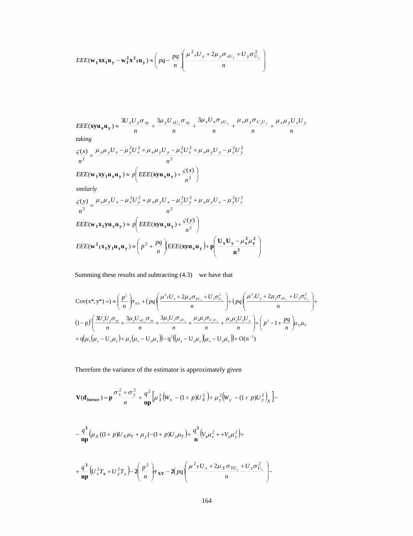
Summing these results and subtracting (4.3) we have that
( ) ( )
( )
( ) ( )( ) ( )( )( ) )n(OUUqUUq
1333
p1
22)*)y,x*(Cov
2xyxyyy
2xyxyyyyx
22
2222
XY
2
−+−−−−+−+
⎟⎠⎞
⎜⎝⎛ +−+⎟
⎟⎠
⎞⎜⎜⎝
⎛++++−
+⎟⎟⎠
⎞⎜⎜⎝
⎛ +++⎟
⎟⎠
⎞⎜⎜⎝
⎛ +++⎟⎟
⎠
⎞⎜⎜⎝
⎛≈=
μμμμμμμμμμ
μμμμσμμσμσμσ
σσμμσσμμσ
YXyxyxUUyxyUxxxyxUyxyyx
UyxUyyxUxYUXxY
npqp
nUU
nn
U
nU
nUU
n
UUpq
nUU
pqnp
yyyx
yyxx
Therefore the variance of the estimator is approximately given
( ) ( )[ ]−+−++−++
=XyyyXxX
yx UpWUpWqn
2222222
)1()1()( μμσσ
nppdV Isrswr
( ) ( )+++++−++− 22)1(()1(( yyzxYyyYXX VVqUpUpq μμμμμμnnp
33
( ) ( ) −⎟⎟
⎠
⎞
⎜⎜
⎝
⎛ ++−⎟
⎟⎠
⎞⎜⎜⎝
⎛−++
n
UUpq
np
TUTUq xx UxYUXxY
yyx
22222 2 σσμμ
σ 22np XYx
3
165
( )
( )
( ) ( )( ) ( )( )( ) )(
333
22
22
2xyxyyy
2xyxyyyyx
2
nOUUqUU2q
p12
122
−+−−−−+−−
⎟⎟⎠
⎞⎜⎜⎝
⎛++++−−
−⎟⎠⎞
⎜⎝⎛ +−−⎟
⎟
⎠
⎞
⎜⎜
⎝
⎛ ++−
μμμμμμμμμμ
μμσμμσμσμσ
μμσσμμ
nUU
nn
U
nU
nUU
npqp
n
UUpq
yxyxUUyxyUxxxyxUyxyyx
YXUyxUyyx
yyyx
yy
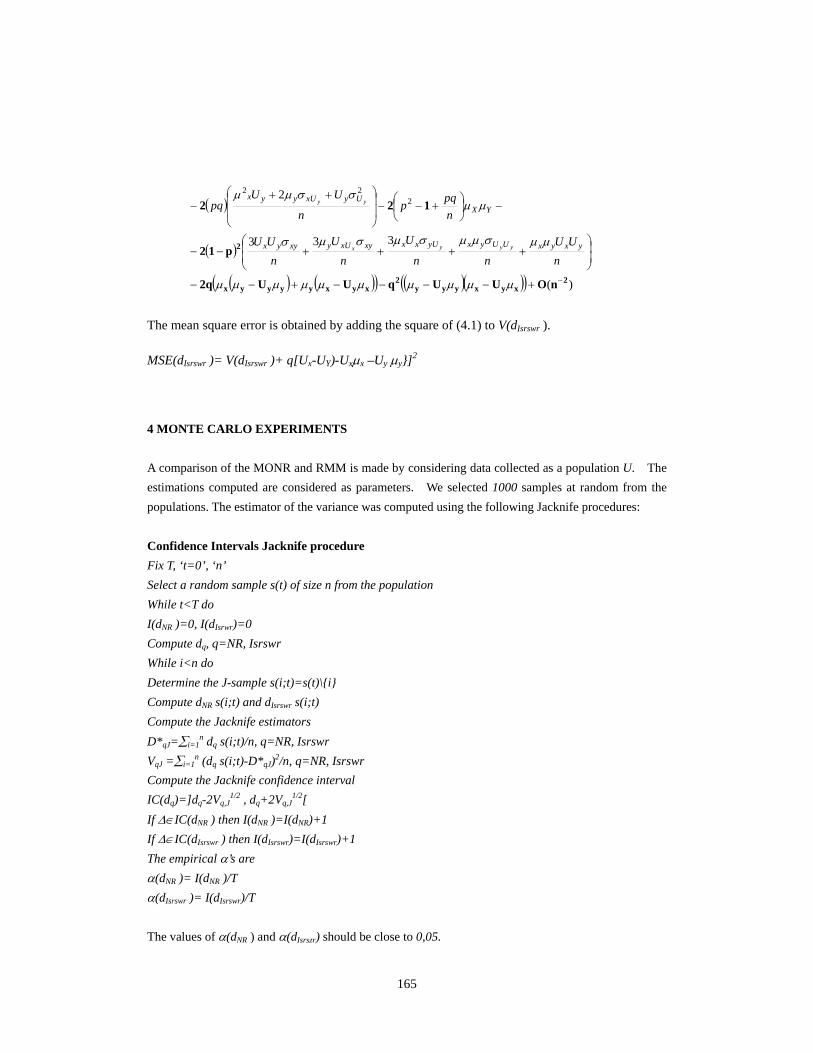
The mean square error is obtained by adding the square of (4.1) to V(dIsrswr ).
MSE(dIsrswr )= V(dIsrswr )+ q[Ux-UY)-Uxμx –Uy μy}]2
4 MONTE CARLO EXPERIMENTS A comparison of the MONR and RMM is made by considering data collected as a population U. The estimations computed are considered as parameters. We selected 1000 samples at random from the populations. The estimator of the variance was computed using the following Jacknife procedures: Confidence Intervals Jacknife procedure Fix T, ‘t=0’, ‘n’ Select a random sample s(t) of size n from the population While t<T do I(dNR )=0, I(dIsrwr)=0 Compute dq, q=NR, Isrswr While i<n do Determine the J-sample s(i;t)=s(t)\{i} Compute dNR s(i;t) and dIsrswr s(i;t) Compute the Jacknife estimators D*qJ=∑i=1
n dq s(i;t)/n, q=NR, Isrswr VqJ =∑i=1
n (dq s(i;t)-D*qJ)2/n, q=NR, Isrswr Compute the Jacknife confidence interval IC(dq)=]dq-2Vq,J
1/2 , dq+2Vq,J1/2[
If Δ∈IC(dNR ) then I(dNR )=I(dNR)+1 If Δ∈IC(dIsrswr ) then I(dIsrswr)=I(dIsrswr)+1 The empirical α’s are α(dNR )= I(dNR )/T α(dIsrswr )= I(dIsrswr)/T The values of α(dNR ) and α(dIsrszr) should be close to 0,05.
166
The data used for establishing the comparisons were selected for, data sets of different research where difference was computed. They ar:e:
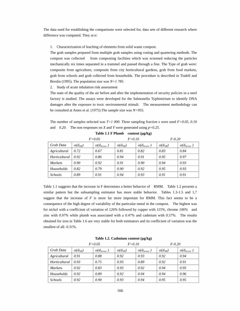
1. Characterization of leaching of elements from solid waste compost. The grab samples prepared from multiple grab samples using coning and quartering methods. The compost was collected from composting facilities which was screened reducing the particles mechanically six times separated in a trammel and passed through a fine. The Type of grab were: composite from agriculture, composite from city horticultural gardens, grab from food markets, grab from schools and grab collected from households. The procedure is described in Tisdell and Breslin (1995). The population size was N=1 785. 2. Study of acute inhalation risk assessment The state of the quality of the air before and after the implementation of security policies in a steel factory is studied. The assays were developed for the Salmonella Typhimirium to identify DNA damages after the exposure to toxic environmental stimuli. The measurement methodology can be consulted at Ames et al. (1975).The sample size was N=955. The number of samples selected was T=1 000. Three sampling fraction s were used F=0.05, 0.10 and 0.20. The non responses on X and Y were generated using p=0.25.
Table 1.1 F Plumb content (µg/kg) F=0.05 F=0.10 F-0.20 Grab Data α(dNR) α(dIsrswr ) α(dNR) α(dIsrswr ) α(dNR) α(dIsrswr ) Agricultural 0.72 0.67 0.81 0.82 0.83 0.84 Horticultural 0.92 0.86 0.94 0.91 0.95 0.97 Markets 0.90 0.92 0.91 0.90 0.94 0.93 Households 0.82 0.79 0.90 0.92 0.95 0.93 Schools 0.89 0.91 0.94 0.93 0.91 0.91
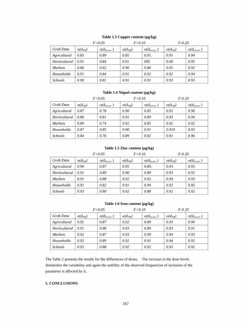
Table 1.1 suggests that the increase in F determines a better behavior of RMM. Table 1.2 presents a similar pattern but the subsampling estimator has more stable behavior. Tables 1.3-1.5 and 1,7 suggest that the increase of F is more far more important for RMM. This fact seems to be a consequence of the high degree of variability of the particular metal in the compost. The highest was for nickel with a coefficient of variation of 126% followed by cupper with 115%, chrome 106% and zinc with 0.97% while plumb was associated with a 0.47% and cadmium with 0.57%. The results obtained for iron in Table 1.6 are very stable for both estimators and its coefficient of variation was the smallest of all: 0.31%.
Table 1.2. Cadmium content (µg/kg) F=0.05 F=0.10 F-0.20 Grab Data α(dNR) α(dIsrswr ) α(dNR) α(dIsrswr ) α(dNR) α(dIsrswr ) Agricultural 0.91 0.88 0.92 0.93 0.92 0.94 Horticultural 0.93 0.75 0.93 0.89 0.92 0.91 Markets 0.92 0.83 0.93 0.92 0.94 0.95 Households 0.92 0.89 0.92 0.94 0.94 0.96 Schools 0.92 0.90 0.93 0.94 0.95 0.95
167
Table 1.3 Cupper content (µg/kg)
F=0.05 F=0.10 F-0.20 Grab Data α(dNR) α(dIsrswr ) α(dNR) α(dIsrswr ) α(dNR) α(dIsrswr ) Agricultural 0.85 0.89 0.85 0.91. 0.91 0.94 Horticultural 0.91 0.84 0.91 095 0.90 0.95 Markets 0.86 0.62 0.90 0.86 0.91 0.92 Households 0.91 0.84 0.91 0.92 0.92 0.94 Schools 0.90 0.81 0.91 0.91 0.93 0.93
Table 1.4 Niquel content (µg/kg) F=0.05 F=0.10 F-0.20 Grab Data α(dNR) α(dIsrswr ) α(dNR) α(dIsrswr ) α(dNR) α(dIsrswr ) Agricultural 0.87 0.78 0.90 0.85 0.92 0.90 Horticultural 0.86 0.81 0.91 0.89 0.93 0.94 Markets 0.89 0.74 0.92 0.85 0.92 0.92 Households 0.87 0.85 0.90 0.91 0.910 0.93 Schools 0.84 0.76 0.89 0.82 0.91 0.96
Table 1.5 Zinc content (µg/kg) F=0.05 F=0.10 F-0.20 Grab Data α(dNR) α(dIsrswr ) α(dNR) α(dIsrswr ) α(dNR) α(dIsrswr ) Agricultural 0.90 0.87 0.95 0.89. 0.93 0.93 Horticultural 0.91 0.89 0.90 0.89 0.93 0.92 Markets 0.91 0.88 0.92 0.92 0.94 0.93 Households 0.91 0.82 0.91 0.94 0.92 0.95 Schools 0.93 0.80 0.92 0.88 0.92 0.92
Table 1.6 Iron content (µg/kg) F=0.05 F=0.10 F-0.20 Grab Data α(dNR) α(dIsrswr ) α(dNR) α(dIsrswr ) α(dNR) α(dIsrswr ) Agricultural 0.91 0.87 0.92 0.89 0.93 0.90 Horticultural 0.91 0.88 0.93 0.89 0.93 0.91 Markets 0.92 0.87 0.93 0.90 0.94 0.93 Households 0.92 0.89 0.92 0.91 0.94 0.92 Schools 0.92 0.88 0.92 0.92 0.93 0.92
The Table 2 presents the results for the differences of doses. The increase in the dose levels diminishes the variability and again the stability of the observed frequencies of inclusion of the parameter is affected by it. 5. CONCLUSIONS
168
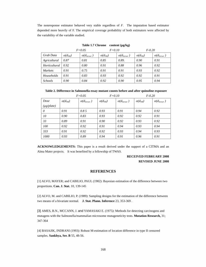
The nonresponse estimator behaved very stable regardless of F. The imputation based estimator depended more heavily of F. The empirical coverage probability of both estimators were affected by the variability of the variable studied.
Table 1.7 Chrome content (µg/kg) F=0.05 F=0.10 F-0.20 Grab Data α(dNR) α(dIsrswr ) α(dNR) α(dIsrswr ) α(dNR) α(dIsrswr ) Agricultural 0.87 0.81 0.85 0.89. 0.90 0.91 Horticultural 0.92 0.80 0.91 0.88 0.96 0.92 Markets 0.91 0.75 0.91 0.91 0.93 0.92 Households 0.91 0.83 0.93 0.92 0.92 0.91 Schools 0.90 0.84 0.92 0.90 0.95 0.94
Table 2. Difference in Salmonella essay mutant counts before and after quinoline exposure F=0.05 F=0.10 F-0.20 Dose (µg/plate)
α(dNR) α(dIsrswr ) α(dNR) α(dIsrswr ) α(dNR) α(dIsrswr )
0 0.91 0.8 5 0.93 0.91 0.94 0.92 10 0.90 0.83 0.93 0.92 0.92 0.91 33 0.89 0.91 0.90 0.92 0.93 0.92 100 0.92 0.92 0.91 0.94 0.93 0.94 333 0.91 0.92 0.92 0.93 0.94 0.93 1000 0.93 0.89 0.94 0.91 0.96 0.91
ACKNOWLEDGEMENTS: This paper is a result derived under the support of a CITMA and an Alma Mater projects. It was benefited by a fellowship of TWAS.
RECEIVED FEBRUARY 2008 REVISED JUNE 2008
REFERENCES [1] ALVO, MAYER; and CABILIO, PAUL (1982): Bayesian estimation of the difference between two proportions. Can. J. Stat. 10, 139-145 [2] ALVO, M. and CABILIO, P. (1989): Sampling designs for the estimation of the difference between two means of a bivariate normal. J. Stat. Plann. Inference 23, 353-369 . [3] AMES, B.N., MCCANN, J. and YAMASAKI E. (1975): Methods for detecting carcinogens and mutagens with the Salmonella/mammalian microsome mutageneticity tests. Mutation Research, 31; 347-364 [4] BASAJIK, INDRANI (1993): Robust M-estimation of location difference in type II censored samples. Sankhya, Ser. B 55, 48-56.

169
[5] BOUZA, C.N. (1981): On the problem of subsample fraction in case of non response. (Spanish) Trab. Estad. Invest. Oper. 32, 30-36. [6] BOUZA, C.N. (1983): Estimation of a difference in finite populations with missing observations . Biom. J. 25, 123-128 [7] CHANDRA, P.; SINGH, H.P. and SINGH, S. (2003): Variance estimation using multiauxiliary information for random non-response in survey sampling. Statistica 63, 23-40.. [8] CHANG, H.J. and HUANG, K. (2001): Ratio estimation in survey sampling when some observations are missing. Int. J. Inf. Manage. Sci. 12, 1-9. [9] CHANG, H.J. and HUANG, K. (2000): On estimation of ratio of population means in survey sampling when some observations are missing. J. Inf. Optimization Sci. 21, 429-436 . [10] CHATURVEDI, AJIT (1986): Sequential estimation of the difference of two multinormal means. Sankhya, Ser. A 48, 331-338 [11] CHOU, R.J. and HWANG, W. L. (1986): Sequential estimation of the difference between two multivariate normal means. Bull. Inst. Math., Acad. Sin. 14, 1-10 [12] DESSIMOZ , C., GIL, M., SCHNEIDER A. and GONNET G.H. (2006): Fast estimation of the difference between two PAM/JTT evolutionary distances in triplets of homologous sequences. BMC Bioinformatics, doi:10.1186/1471-2105-7-529. [13] FROLKING, S., QIU, J., BOLES, S., XIAO, X., LIU, J., LI, C., and QIN X. (2002): Combining remote sensing and ground census data to develop new maps of the distribution of rice agriculture in China, Global Biogeochemical Cycles, (16 1091, doi:10.1029/2001GB001425). [14] FUTATSUYA, M. and TAKAHASI, K. (1979): Interval estimation of the difference of the parameters of two lognormal distributions based on sample means. (Japanese), Sci. Rep. Hirosaki Univ. 26, 39-48 [15] GERMAIN, M. and SCANDURA, T. (2005). Grade Inflation and Student Individual Differences as Systematic Bias in Faculty Evaluations. Journal of Instructional Psychology, 32, 58-67. [16] GHOSH, M. and MUKHOPADHYAY N. (1980): Sequential point estimation of the difference of two normal means. Ann. Stat. 8, 221-225 [17] GUO, B., LEE, D., XU, W., DAVIS, D., and LUO, M. (2006) Quantitative expression analysis of adversity resistance genes in corn germplasm with resistance to preharvest aflatoxin contamination. Proceedings of the 18th Annual Multi-Crop Aflatoxin Elimination Workshop, Raleigh, North Carolina..
170
[18] HAYRE, L.S. (1983): Sequential estimation of the difference between the means of two normal populations. Metrika 30, 101-107 . [19] KELLEY, THOMAS A. (1977): Sequential Bayes estimation of the difference between means. Ann. Stat. 5, 379-384 [20] KHARE, B.B. and SRIVASTAVA, S. (1993): Estimation of population mean using auxiliary character in presence of non-response. Natl. Acad. Sci. Lett. 16, , 111-114. [21] KLEMZ, B.R., (1999): Assessing contact personnel/ customer interaction in a small town: differences between large and small retail districts. Journal of Services Marketing. 13. 194 - 207 [22] KULIK, J., CHEN-LIN A. , KULIK, C. and COHEN P.A.(1998):Effectiveness of Computer-based College Teaching: A Meta-analysis of Findings. Review of Educational Research, 50, 525-544. [23] LIN, P. E. (1971): Estimation procedures for difference of means with missing data. J. Am. Stat. Assoc. 66, 634-636.. [24] LUI, K. J. (1999): Interval estimation of simple difference under independent negative binomial sampling. Biom. J. 41, 83-92 .. [25] LUI, K. J. (2001): A note on interval estimation of the simple difference in data with correlated matched pairs. Biom. J. 43, 235-247. [26] MARTINELLI, D. ,GROSSMANN, G. SÉQUIN, U. , BRANDLAND H. and BACHOFEN R. (2004): Effects of natural and chemically synthesized furanones on quorum sensing in Chromobacterium violaceum. BMC Microbiology 2004, 4:25doi:10.1186/1471-2180-4-25 (The electronic version of this article is the complete one and can be found online at: http://www.biomedcentral.com/1471-2180/4/25). [27] MOORE, S.A., LENGLET, A. and D HILL, N. (2002): Field evaluation of three plants based insect repellents against malaria vectors. VACA diE2 Province of the Bollivian Amazon. J Am Mosq Cont Assoc 18: 107. [28] MUKHOPADHYAY, N. and DARMANTO, S. (1988): Sequential estimation of the difference of means of two negative exponential populations. Sequential Anal. 7, 165-190 [29] MUKHOPADHYAY, N. AND PURKAYASTHA, S. (1994): On sequential estimation of the difference of MEANS. Stat. Decis. 12, 1, 41-52 . [30] MYOUNG-JAE (2005): Monotonicity conditions and inequality imputation for sample-selection and non-response problems. Econ. Rev. 24, 175-194.. [31] OWE M. and D'URSO G. (2002): Remote Sensing for Agriculture, Ecosystems, and Hydrology III. Proceedings of SPIE Volume 4542
171
[32] PINNOI, A., LUMYONG, S., HYDE, K.D. and D JONES, E.B.G. (2006). Biodiversity of fungi on the palm peat swamp forest, Narathiwat, Thailand. Fungal Diversity 22, 205-218. [33] REKAB, KAMEL (1992): Bayesian estimation of the difference between two mean times to failure. Stochastic Anal. Appl. 10, 343-350. [34] RUEDA, M,. MARTÍNEZ, S. MARTÍNEZ H. and ARCOS, A. (2006q): Mean estimation with calibration techniques in presence of missing data, Computational. Statistics. And Data Analysis, 50, 3263-3277. [35] RUEDA, M,.GONZÁLEZ, S.. and ARCOS, A. (2006b): A general class of estimators with auxiliary information based on available units. Applied Mathematics. and Computation., 175, 131-148. [36] RUEDA, M. and GONZÁLEZ, S. (2004) Missing data and auxiliary information in surveys, Computational. Statistics. 10, 559-567. [37] SINGH, RANDHIR, C. M. KISHTAWAL and D P. C. JOSHI (2005): Estimation of monthly mean air-sea temperature difference from satellite observations using genetic algorithm. Geophysical Res. Letters, 32, [38] SILVERMAN, A.Y., S. L SCHWARTZ AND R. W STEGER (1982): A quantitative difference between immunologically and biologically active prolactin in hypothyroid patients. Journal of Clinical Endocrinology & Metabolism, 55, 272-275 [39] SINGH, S.; JOARDER, A.H. and TRACY, D.S. (2000): Regression type estimators for random non-response in survey sampling. Statistica 60, 39-44. [40] SCHRECK, C.E. and LEONHARDT, B.A. (1991): Efficacy assessment of Quwenling, a mosquito repellent from China. J Am Mosq. Cont Assoc 7: 433.. [41] SHUKLA, D. and DUBEY, JAYANT (2000): A new sampling scheme for coping complete non-response in sample surveys. Appl. Sci. Period. 2, 85-89. [42] TISSDEL, S.E. and BRESLIN V. T; (1995): Characterization of leaching of element from municipal solid waste compost. J. of Environmental Quality. 24, 827-833 [43] TRYBULA, STANISLAW (1991): Estimation of the difference of parameters. Statistics, 22,199 - 204 [44] TSUKERMAN, E.V. (2004): Optimal linear estimation of missing observations. (Russian) Studies in information science. Kazan: Izd. Otechestvo. 2, 75-96.. [45] WURST, J., NETER, J. and GODFREY, J. (1991). Effectiveness of rectification in audit sampling.

172
The Accounting Review, 66, 333-346. [46] XIAO, X., J. LIU, D. ZHUANG, S. FROLKING, S. BOLES, B. XU, M. LIU, W. SALAS, B. MOORE, and C. LI, (2003): Uncertainties in estimates of cropland area in China: A comparison between an AVHRR-derived dataset and a Landsat TM-derived dataset. Global and Planetary Change, 37: 297-306 [47] ZOU, G. and D FENG, S. (1998). Sample rotation method with missing data. The 4th ICSA Statistical Conference, Proceedings, Kunming. [48] ZOU, G., FENG, S. and QIN, H. (2002). Sample rotation theory with missing data. Science in China Ser. A, 45, 42-63.


