~~';,~-

Optimization of discrete arrays of arbitrary geometryRoy L. Streit

New London Laboratory. Naval Underwater Systems Center, New London, Connecticut 06320(Received 20 November 1979: accepted for publication 4 October 1980)

The concept of Directivity Index with Beamwidth Control (DIBC) leads to a practical method for theoptimization of element excitations to control the tradeoff between beamwidth and sidelobe level in a discretearray of arbitrary configuration. This optimization procedure depends on the design frequency, specifiedelement positions, individual element field patterns, and ambient noise field. Each of these factors can bespecified in a completely general manner. In addition, the optimization procedure can be adapted tocomputers of modest memory size by using subarrays of the full array. Examples are included to show theversatility of this approach to the optimization problem, as well ~s its limitations. One of these examples is alOS-element cylindrical array. '

PACS numbers: 43.60.Gk, 43.30.Vh, 43.28.Tc

I. THE CONCEPT (4) The ambient noise field at the design frequency isA 1 ad . completely known.. ntr uctlon

(5) Element interactions can be ignored.Optimization of the element excitations of discreteantenna arrays is a matter of definition for three rea- (6) Element excitations can be phased (i.e., complex).sons. First, the definition of optimality will dictate Th . th t th 1 t C.tat . S mu t be ale prem1se a e e emen ex I Ion s -the appropriate mathematical approach. Seemingly 1 d t be h d . t Y As .s po.nted outowe 0 p ase IS no necessar. I 1subtle changes in the definition of optimality can alter 1 t . t ' I . th to be str1.ctl. . . a er, we can Jus as easl y require em yradically the applicable mathemat1cal methods. Second, 1 . .th .t . t . Hrea, I.e., e1 er posllve or nega 1ve. owever, ex-element excitations that are optimal in one sense are t h t d th t th .t t .cep were no e , we assume a e eXC1 a IOns areunlikely to be optimal in another sense. Two sets of h d be th '. th 1 .t t . d. . . .. p ase cause IS IS e more genera Sl ua 10n anexc1tat1ons, each set optimal m 1tS own sense, can be

11 f bett f1 t 1 d.ff t Th .rd th d f . .t . f t . 1 a ows or er per ormance.comp e e y 1 eren. 1, e e 1n1 Ion 0 op Ima -ity must reflect directly on the primary design goals The concept of DIBC has been defined and used earlierf~r the array. It is pointless t~ optimize t~e Directi- by Butler and Unz .1, 2 In these papers, DIBC is calledvlty Index (DI) and then complaIn that the side lobes are beam efficiency and is defined by them only for linet~o hig?,. ~cause t~e de.sign go~ of low sidelobes ~nd arrays. This article is new in three regards. First,t e def1n1t1on of optlmality (max1mum DI) are not dl- we apply the concept of DIBC to arbitrary spatial ar-rectly related. rays and, thereby demonstrate its usefulness in very

This article defines and uses exclusively the con- general situations. Second, we exhibit viable numericalcept of Directivity Index with Beamwidth Control procedures and techniques for overcoming a variety of(DiOC). Several advantages, as well as difficulties, mathematical difficulties inherent in the concept ofinherent in this definition are discussed. The primary maximizing DIBC. Third, the above-mentioned methoddifficulty in this definition is the requirement of large of optimizing DIBC for general spatial arrays of anycomputer memories for large arrays. A technique number of elements, while using only small amountsemploying subarrays of the full array in a systematic of core storage (and no peripheral storage devices),manner is shown to overcome this problem. The same appears to be completely novel to this article.technique can be used to solve the following problem as All th 1 . th O t . 1 t d. . . . e examp es m 1S ar 1C e were compu e onwell: Given an array w1th known element posItions and th U ' 1108 d EXEC 8 A I ' t ' f th. . e nlvac un er . 15 mg 0 e com-exc1tatlons, and given t?at new elements are t~ be in- puter program is available in Streit.3 It is written intr~uced at known locations, ?OW does one excite (or FORTRAN V for the general three-dimensional arraydrive) these new elements to 1mprove performance of of arbitrary configuration.the total array without changing the excitations of anyof the elements of the original array? B F. Id d rd .. Ie patterns an coo Inate system

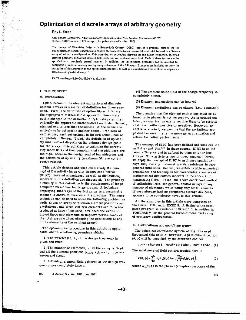
The optimization procedure in this article is appli- Th h . I d. t t f F. 1 . d. '. e sp erlca coor ma e sys em 0 19. 15 usecable when the folloWIng prem1ses obtaIn: th h t th ' t ' 1 h t . 1 d. t .roug ou 1S ar IC e; owever, a par 1CU ar Irec Ion(1) The wavelength, ~, of the design frequency is (9,.p) will be specified by the direction cosines

given and fixed. . '" ". '" . '"(1)cosa = sm", coS9, cos... = sm", sm9, cosy = cos'" .

(2) The number of elements, n, in the array is fixed Th t 1f . Id tt t t d h . . . e mos genera 1e pa ern rea e ere ISand all the element POSItiOns (x_,y-,z.), k= 1,...,n areknown and fixed. V(9,.p)= t a,.R_(9,.p)exp(~d_(9,.p)), (2)

(3) Individual element field patterns at the design fre- .1

quency are completely known. where R.(9,.p) is the phased (complex) response of the

199 J. Acoust, Soc. Am. 69(1), Jan. 1981 199-

"

-43-

~~--

Z of the ratio (4a), and this proves our assertion. This is

not to say, of course, that the maximum value of (4)and the maximum value of (4a) are equal, only {hat ex-citations that maximize the one also maximize theother.

Maximizing DI is a limiting case of maximizing DIBC.Y To see this, recall that for a specified direction

(Bo, CPo)' DI is a maximum if the ratio

DI= N(Bn,CPn)IV2(Bn,CPn)1 (5)

x I1N(B,cp)IV2(B,CP)ISinCPdCPdB'n

FIG. 1. The coordinate system.is maximized. Now let the ignored region 8 be empty,let the mainlobe region, m, contain (Bo' CPo), and let

kth element, and S=.I1 -m, Then, excitations maximizing DIBC con-d (B "' ) " (3) verge to excitations that maximize DI as the mainlobe

'I' =x cosa+v coS...+z cosy. ,-, - - - regIon, m, shrinks down on the point (Bo, CPo)'

Because of assumptions (1) to (6), the field pattern W h d f ' d t " 1 " t t ' th f. eave e me op lma eXCl a Ions as ose orY(B, CP) depends solely on the phased (complex) exclta- h ' h DIBC ' " d f h ' f ', , ,w lC IS maxImIze or some c olce 0 regIons

tIonsa"...,an. The ambIent noise field N(B,cI»wIll om" d8 Th '11 f t 1, . , . . ,. 01", 0, an . IS a ows a measure 0 con ro over

enter rn the dehmtIon of optimal excItatIons. [Alter- th be 'dth d ' d 1 be 1 1 B 't, , ,e amWl an Sl e 0 eve. y varYIng sys ema-

nately, one may think of N(B,CP) as a gIven non-negatIve t ' 11 th h ' f om d " d ""th DIBC" , lca y e c Olce 0 01" an 0 an maxImIzIng e

weIghtIng functIon of the two angles.] f h h ' , d 'tl th t ad ffor eac c olce, we can examIne lrec y e r eo

C. Directivity index with beamwidth control (DISC) between beamwidth and sidelobe level for the particulararray at hand. The engineer can, then, select those excita-

The antenna designer is required to divide the set of t ' th t be t ' t h ' d G 11 th 1lId ' t ' d td .l1' h d '", IOns a s SUI lsnees. eneray, eargera lrec Ions, eno e ,mto tree lsJornt regIons: th ' 1 be ' om d th 11 th ' d 1 bee maIn 0 regIon, 01", an e sma er e Sl eo

m= mainlobe region, region, S (for fixed ignored region, 8), the lower the" . d 1 be ' overall side lobe level and the greater the beamwidth.o=Sl eo region , However, this may not always be the case, since side-

8 = ignored region = .11 - (m US) . lobe level does not enter directly into the DIBC ratioTh ' d ' " f d ' t ' 1 ' 1 t 1 of (4). Nothing prevents the field pattern from havingIS lVlSlon 0 Irec lona space IS comp e e y ar- " "

b Ot t th t .th om " be t ts narrow high amplItude side lobes , sInce such sidelobesI rary, excep a nel er 01" nor 0 can emp y se '. , ,h 8 be t ' f d ' d 0 t ' 1 contrIbute lIttle to the Integral m the denominator ofw ereas can emp y 1 eslre. nce a par ICU ar th D

choice of~, S, and 8 has been made, the following def- e IBC.

inition of optimality is used. Another reason for maximizing DIBC is simply that

Definition 1 The element excitations a" . . . ,an are it is conceptually easy to do so. All that is ~equired isoptimal excitations for a given choice of regions m, S, the solution of an eigenvalue/eigenvector problem (seeand 8 if and only if the ratio Theorem 1), and problems of this type have been studied

extensively in the literature.' Numerically, suchILN(B,CP)ly2(B,cp)ISinCPdCPdB problems require considerable care. Fortunately,

DIBC = (4) well-designed computer programs are available for theJ f N(B,CP)ly2(B,cp)lsincpdcpdB solution of eigenproblems.5.. With the use of these rou-

!!!tV S tines, the solutions of the eigenproblems encounteredis maximized, Any ratio of this form will be referred in the antenna problem seem to be numerically stable.to as a directivity index with beamwidth control. This is not to say that there may not be arrays that

yield numerically unstable eigenproblems.We point out that any excitations a" . . . , an that max-

imize the DIBC ratio (4) also maximize the ratio A final reason for maximizing DIBC is more esoteric.r r In the process of solving the required eigenproblem,

JiOJIIoN(B,t/»ly2(B,cp)lsinCPdt/>dB. (4a) all the eigenvalue/eigenvector pairs are computed, notf merely the largest one. It happens that the field pat-h N(B, t/»1 Y2(B, CP)I sincp dt/> dB terns corresponding to the lower order eigenvalues

have some interesting features [see the figures in ex-To see this, note that ample (2)]. In addition, it often happens that some of

. Ii 11 the larger eigenvalues are close together; i.e., sev--!-=~= 1 + -2 erallinearly independent sets of excitations existDIBC I h 1.£ ' which give DIBC values that lie close together. (For

3It 91t an analogous situation, see Slepian and Pollak. 7) What

so that any excitations minimizing the reciprocal of this means in the antennna problem is that, withoutDIBC are also excitations that minimize the reciprocal sacrificing antenna performance (as measured solely

200 J, Acou5t, Soc, Am" Vol, 69, No, 1, January 1981 Roy L, Streit: Discrete arraY5 of arbitrary geometry 200

-44-

.'by the DIBC), it becomes a simple matter to examine elements in the array. Make any initial guess at thenumerous different sets of excitations with the aim of optimal excitations. Define distinct subarr;tys of, say,improving some completely different design goal of 50 elements each. By working with the first of thesethe array" [See (19) below.] This will not be discussed subarrays, new element excitations are computed forfurther in this article. these 50 elements, so that the DIBC of the entire 300

t b t. d th t th o h t th element array is increased. Next, new excitations areIt mus e men lone a IS approac 0 e array "t " ' t " bl d t tt t t dd computed for the second subarray. Cycling through allop Imlza Ion pro em oes no a emp 0 a ress sev-, "" .

1 " th t f t " 1 " t t F " t th ' SIX subarrays In turn, until DIBC for the entire 300 ele-era Issues a are 0 prac Ica In eres" Irs, IS t t b ' d f th b h " thmen array canno e Increase ur er y c anglng eapproach does not guarantee that the array performance " t t '" f th b " th f"" " , '""" exci a IOns In any 0 e su arrays IS e essence 0IS insensItive to perturbations In the optimum exclta- d" t 1 t " Th '

thod be dt. Th t ' { , " , " t t " t group coor Ina e re axa Ion. e me can proveIons. e ques Ion 0 sensitivity to exci a Ion per ur- t be t It " Id th 1 b 11 be t "" . ., 0 convergen. Yle s ego a y s exclta-batlon can be examined only after the optimum exclta- t ' t 1 1 11 be t A f 1 t t t f' , Ions, no mere y oca y s. care usa emen 0tlons are found. Second, this approach does not attempt th 1 ' th d f th k '. th b' e a gorl m an ur er remar s are given In e su -to control the efficiency of the array. In other words, t " , 1 1 t " f th ' bl b" ". ,sec Ion on numerlca so u Ion 0 e elgenpro em yit can happen that the optimal excitations for a partl- th " d " t thodd " " i h ' e In Irec me .cular array may rive certain e ements at t elr max-imum allowed levels while the remaining elements are The rate of convergence of the group coordinate re-hardly driven at all, so that the total output power of laxation method depends heavily on the size of the sub-the array is too low for the application. This problem arrays used. The larger the subarrays, the faster theis common to all amplitude shaded arrays and can be convergence, and the more core storage required.examined after the optimum excitations are found. Thus, core storage is traded off in a direct manner forFinally, this approach to array optimization ignores the convergence rate and, hence, for computation time.element interactions, so that it is possible for optimum In addition, each step of the group coordinate relaxationexcitations derived by this method (or by any other method produces new excitations that increase themethod for that matter) to have undesirable character- DIBC, so that if the computations are interrupted foris tics in this regard. This possibility, as well as the any reason: (1) The last computed excitations areother two possibilities mentioned above, should be in- better than any of the excitations previously computedvestigated after optimal excitations are found, and (2) by saving the last computed excitations, the

computations can be resumed without significant loss.D. Computer storage problem If n. is the number of elements in a subarray used

The primary drawback to maximizing DISC is that by the group coordinate relaxation process, the totalthe number of computer storage locations required storage required (using the program in Streit3) is ap-(using the program in Streit3) is approximately proximately

NT=6n2+16n+12000words, (6) NlI=6n~+8(n+n.)+12000words, (7)

for the case of constant ambient noise field and omni- for the case of constant ambient noise field and omni-directional elements. Since the total requirement will directional elements. Thus, memory requirementsgrow as the ambient noise field and/or element field grow as the square of the subarray size no matter howpatterns require more storage to compute, it appears large the full array may be. By choosing the subarraythat the direct computation of optimal excitations for size sufficiently small, the designer can maximizeany array of 100 or more elements requires either DIBC for large arrays on computers of modest size.large main-frame computers or computers with virtual The cost, however, is computer time. On the othermemory. However, the storage requirements for hand, if the designer has a dedicated minicomputer ofmaximizing DIBC can be avoided. A technique known reasonable size, the cost of computer time is nil.as group coordinate relaxation" gives a method that canbe tailored to the computer memory available. Thetechnique is an excellent example of how to trade off Icomputer memory for computational speed. The more I. ELABORATION OF THE CONCEPT

memory available, the faster the DIBC can be maxi- A. DIBC and the eigenproblemmized.

Let the vector a= (al,... ,a.)T be the vector of elementGroup coordinate relaxation, in the context of maxi- excitations for the field pattern V(O,t/» given by (2).

mizing DIBC, is simply stated. Suppose there are 300 Then, I

fJJltN(O,t/»IV2(O,t/»ISint/>dt/>dO= fl N(O,t/»IV(9,t/»12sint/>dt/>dfJ "

= !.£nN(9,t/» [h a.R_(9,t/»exP(~d_(9,t/»)] [kaJRJ(9,t/»exp(~dJ(9,t/» )]Sint/> dt/> d9

= ~I t ii_aJ! .LN(9,t/>~RI(9,t/»exp(~[dJ(9,t/»-d_(9,'ttI)ijsint/>dt/>d9=iiTUa, (8)

201 J" Acoust" Soc. Am", Vol. 69, No, 1, January 1981 Roy L" Streit: Discrete arrays of arbitrary geometry 201

.,

-45-

-~- ---~ ~--~~-~-

where U is an n x n complex matrix. If U = (,/.,], with " (~ ) = (18)

k denoting the row number and j denoting the column n::~ zTIVz /Jon,

number, then d th O "" ' tt ' d f ' ctan lS mmlmum lS a ame or every elgenve orf " r corresponding to /Jo. Finally, if 1 ~ k ~ n, then, foru.,= J~ N(9, 4»R ,(9, 4»R.(9, 4» any constants al" .n. ,a. not all zero, we have

x eXP(-?T[d,(9,4»-d.(9,4»])sin4>d4>d9. (9) ./JoI" ZTUZ/ZTWz" /Jo., (19)

wheret=alz,+...+a.z..Clearly,UisaHermitianmatrix(i.e.,U=UT),since Th f fth ' t fth ' th". - " , , , e proo so e varlOUS par SOlS eorem canIt lS obvIous that u.,=1/,.. Also, U lS posltive definIte, be f d ' g Gantmacher 4oun m numerous sources, e. ., .since

For the immediate purposes, the most importantaTUa= If N(9,4»ly2(9,4»lsin4>d4>d9> 0, (10) part of this theorem is (17), It states that optimal ex-~ citations are precisely the components of any eigen-

whenever the excitation vector a* 0 (and provided the vector corresponding to the largest eigenvalue of themainlobe region, ~, is not a set of measure zero, a generalized eigenproblem Uz = }J.Wz, where U and ~Vpathological condition that is not encountered in this are defined by (9) and (12).application), Therefore, for every mainlobe region, Th t " 11 Th 1 1 th bl of ax' " , , eore lca y eorem so ves e pro em m -~, the matrix U dehned m (9) lS an n x n posltive def- '"

DIBC " th h 11 1 t ' t t . lmlzmg m e case were a e emen eXCl a lons

inite Hermitian matrix. Similarly, b h d B t h t ' th 1 t ' ' f 11th ' can e p ase. u w a lS e so u lon 1 a e excl-

f -r N(9 4» ly2(9 4»lsin4>d4>d9=aTWa (11) tations are required,to be re~l (positive or negati~e)?J~ua" 'In this case, the ratlo (13) still holds, but the exclta-

, , , . . , " tion vector, a, is real, i.e., a=a, Since U and Warewhere W = [w.J ] lS an n x n posltive dehmte Hermltian H ' t " h th 1 b ' ' d t ' terml lan, we ave e a ge ralc 1 en 1 ymatrix whose general entry is

DIBC=~=~~. (20)w.,= f . r N(9,4»R,(9,4»R.(9,4» a Wa a (ReW)a

J~ua2 ' Now, ReU and Re Ware both real symmetric matrices,

x exp( ;.!! [d ,(9,4» -d.(9, 4> )])sin4> d4> d9 . (12) and all the properties of Theorem 1 hold for the real~ generalized eigenproblem (ReU)z = }J.(ReW)z, The only

Thus, for a given choice of~, S, and 8, we have difference is that now the eigenvectors have all real

components. Therefore, if the excitations are requiredDIBC=aTUa/jjTWa, (13) to be real, the optimal real excitations are precisely

" , , , , , , . the components of any eigenvector corresponding to "theWhlCh IS a ratio of posltive dehmte Hermltian forms. 1 t ' 1 f th I ' d 1 . np obI m" arges elgenva ue 0 e genera lze rea elge r e

Therefore, optimal excitations are those that maxlmlze

this ratio of Hermitian forms. (ReU)z = }J.(ReW)z , (21)

The mathematical tools for handling ratios of the. where U and Ware the matrices defined by (9) and (12).form (13) have been known for at least a century. I th . d f thO t '

1n e remain er 0 lS ar lC e, we concern our-We have the following general mathematical result. 1 1 ' th h d ' t ' E th ' th tse ves on y Wl P ase exclta 10ns. very mg a

Theorem 1: If U and Ware n x n Hermitian matrices we do, however, can be recast for real excitationsand W is positive definite, then the eigenvalues of the simply by using the real parts of the matrices involved.generalized eigenproblem "'" ,

A dlscrete reformulation of DIBC lS dlscussed m theUz= }J.Wz (14) next section. By way of analogy only, this discrete

, version of the DIBC ratio is to DIBC as the discreteare all real. Let}J.,;'}J.2;"""}J.n denote these elgen- F ' t f ' t th F ' t f F 1. , ourler rans orm lS 0 e ourler rans orm. 0-values. Then, 11nearly independent vectors Zl"" ,zn 1 , th '. d ' , f th ' 1 thodbe d th t t' f OWing 1S 18 a lSCUSS10n 0 e numer1ca me scan foun a sa lS y for the solution of the kind of eigenproblems encounter-

Uz.=}J..Wz., k=I,...,n, (15) edinthisarticle.

andB. A discrete version of DIBC

-T { I, if k=j(16)z. Wz,=. Maximizing the DIBC ratio (4) is mathematically

0, if k* j tractable, but it is not practical. It requires the solu-

The vectors z I' . . . ,zn are called the eigenvectors of tion of an eigenproblem, which in turn requires thethe eigenproblem (14). Also, we have evaluation of approximately n2 double integrals (9) and

-T (12) over subsets of the unit sphere. Since it is essen-max (~) = }J., , (17) tial that the mainlobe region, ~, and the sidelobe re-"0 z Wz gion, S, be quite general in nature (i.e., be defined to

and this maximum is attained for every eigenvector suit the particular application, these double integralscorresponding to }J.I' and are in general impossible to evaluate explicitly and are

202 J, Acoust. Soc. Am., Vol, 69, No, 1, January 1981 Roy L, Streit: Discrete al:rays of arbitrary geometry 202

"

-46-

~,~

i P EQUAL "';(£\ 'Q",' PARTS

Y \. .~.-.I

P EQUAL PARTS

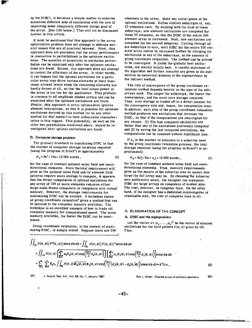
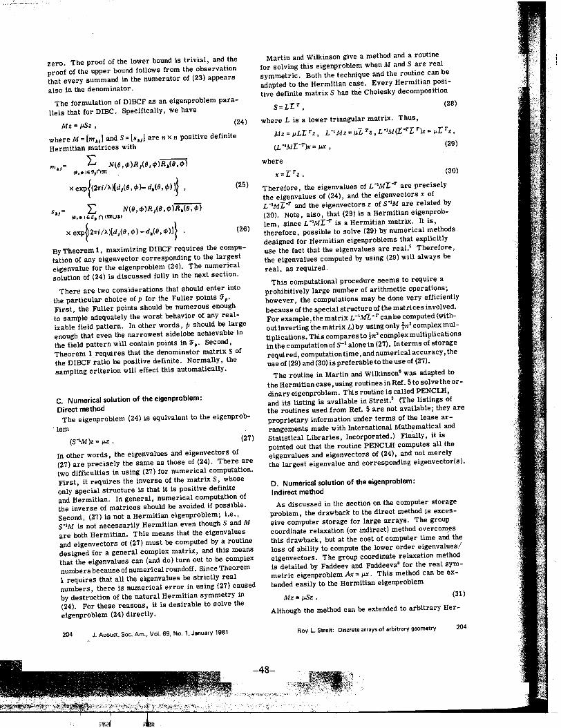
FIG. 3. One face of Icosahedron subdivided Into p ~rts.

.

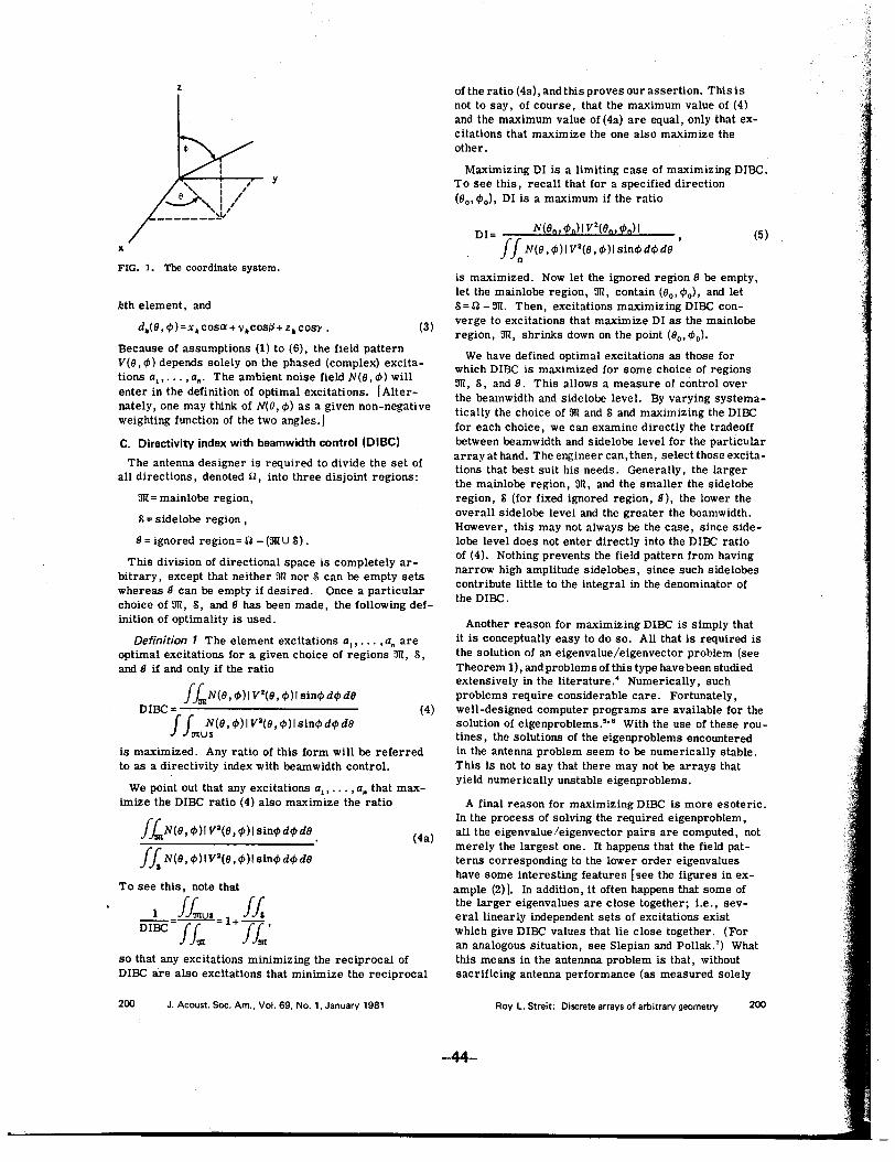
. desic dome of order p. We define the Fuller points,

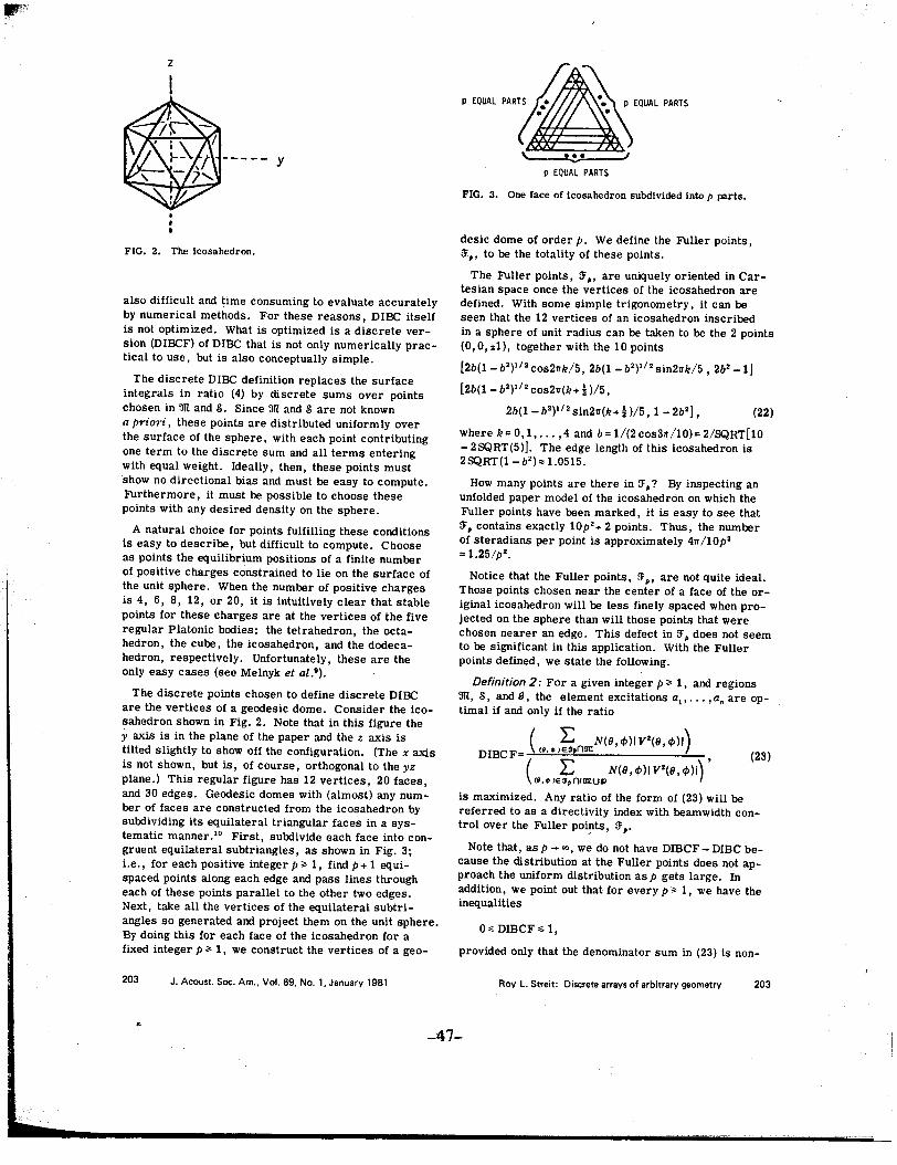
FIG. 2. The Icosahedron. 11" to be the totality of these points.

The Fuller points, ff" are uniquely oriented in Car-tesian space once the vertices of the icosahedron are

also difficult and time consuming to evaluate accurately defined. With some simple trigonometry, it can beby numerical methods. For these reasons, DIBC itself seen that the 12 vertices of an icosahedron inscribedis not optimized. What is optimized is a discrete ver- in a sphere of unit radius can be taken to be the 2 pointssion (DIBCF) of DIBC that is not only numerically prac- (0,0, %1), together with the 10 pointstical to use, but is also conceptually simple. [2b(1-b2)1/2cos211k/5, 2b(1-b2)'/2sin211k/5, 2b2-1J

The discrete DIBC definition replaces the surface [2b(1 - b2)1/2 2 ( !. )/5integrals in ratio (4) by discrete sums over points cos 11 k+ 2 ,chosen in:m and S. Since ~ and S are not known 2b{1-b2)1/2Sin211(k+!)/5, 1-2b2J, (22)a priori, these points are di~tributed u~iformlY .ove.r where k= 0, 1,. . . ,4 and b = 1/(2 COS311 /10)= 2/SQRT[10the surface of the sphere, with each pOInt contributIng 2SQ (5)J Th d I gth f th " h d .. . - RT . e e ge en 0 IS Icosa e ron ISo~e term to the dIscrete sum and all term~ enterIng 2SQRT(1- b2) '= 1.0515.wIth equal weIght. Ideally, then, these pOInts mustshow no directional bias and must be easy to compute. How many points are there in ff,? By inspecting anFurthermore, it must be possible to choose these unfolded paper model of the icosahedron on which thepoints with any desired density on the sphere. Fuller points have been marked, it is easy to see that

A t I h . f . t f If .II ' th nd .t . ff, contains exactly 10p2+ 2 points. Thus, the numberna ura c Olce or porn SUI Ing ese co 1 Ions " 2. eas t desc .be b t d ' ff " It t t Ch of steradians per point IS approxImately 411 /10pIS Y 0 rI, u 1 ICU 0 compu e. oose 2as points the equilibrium positions of a finite number '= 1.25/p .of positive charges constrained to lie on the surface of Notice that the Fuller points, ff" are not quite ideal.the unit sphere. When the number of positive charges Those points chosen near the center of a face of the or-is 4, 6, 8, 12, or 20, it is intuitively clear that stable iginal icosahedron will be less finely spaced when pro-points for these charges are at the vertices of the five jected on the sphere than will those points that wereregular Platonic bodies: the tetrahedron, the octa- chosen nearer an edge. This defect in ff, does not seemhedron, the cube, the icosahedron, and the dodeca- to be significant in this application. With the Fullerhedron, respectively. Unfortunately, these are the points defined, we state the following.only easy cases (see Melnyk et al."). D ". .. 2 " 1 .e,tmtton : For a gIven Integer p;;, ,and regIons

The discrete points chosen to define discrete DIBC ~, S, and S, the element excitations aI, . . . ,an are op-are the vertices of a geodesic dome. Consider the ico- timal if and only if the ratiosahedron shown in Fig. 2. Note that in this figure they axis is in the plane of the paper and thez axis is ( L N(9,tf»IV2(9,tf»I)tilted slightly to show off the configuration. (Thexaxis DIBCF= \ (e.o)E;;-,n91t"\V""", \V"""I, (23)is not shown, but is, of course, orthogonal to theyz ( L N(9,tf»IV2(9,tf»i)plane.) This regular figure has 12 vertices, 20 faces, (e.O)E:J,n(91tul>and 30 edges. Geodesic domes with (almost) any num- is maximized. Any ratio of the form of (23) will beber of faces are constructed from the icosahedron by referred to as a directivity index with beamwidth con-sutxlividing its equilateral triangular faces in a sys- trol over the Fuller poi!;lts, ff,.tematic manner.lo First, sutxlivide each face into con-gruent equilateral subtriangles, as shown in Fig. 3; Note that,. as? -~, we do not have ~IBCF-DIBC be-i.e., for each positive integer p;;, 1, find P + 1 equi- cause the dis~nbutio~ at .the .Fuller pOInts does not ap-spaced points along each edge and pass lines through pro~~h the umf~rm dIstrIbutIon as p g~ts large. Ineach of these points parallel to the other two edges. ~dItIO~,. we pOInt out that for every p - 1, we have theNext, take all the vertices of the equilateral subtri- InequalItIesangles so generated and project them on the unit sphere. 0 ~ DIBCF ~ 1By doing this for each face of the icosahedron fora '

fixed integer p;;, 1, we construct the vertices of a geo- provided only that the denominator sum in (23) is non-

I203 J. Acoust. Soc. Am., Vol. 69, No.1, January 1981 Roy L. Streit: Discrete arrays of arbitrary geometry 203

" -47-

zero. The proof of the lower bound is trivial, and the Martin and Wilkinson give a method and a routine ,proof of the upper bound follows from the observation for solving this eigenproblem when?-1 and S are real -:

that every summand in the numerator of (23) appears symmetric. Both the technique and the routine can be

also in the denominator. adapted to the Hermitian case. Every Hermiti~ posi-Th f 1 t . f DIBCF . bl tive definite matrix S has the Cholesky decomposition

e ormu a lon 0 as an elgenpro em para-llels that for DIBC. Specifically, we have S = LI T , (28)

Mz = fJSz , (24) where L is a lower triangular matrix. Thus,where M = [m.IJ and S= [S.I] are n x n positive definite A1z = jJ.LL TZ, L -I ,,"lz = III Tz ,L -1M (r-TL T)Z = jJ.I T z,

Hermitian matrices with (L -1?-lL-T)x = jJ.X (29)1:: '

m.l= N(8,I/»RI(8,I/»R.(8,1/» where(9,- IE\J,nmI x = L T Z . (30)

x exp{ (21Ti/X)[d (8 1/»- d (8 "') J} (25) - I' .' 'I' , Therefore, the eigenvalues of L -'ML -T are precisely

the eigenvalues of (24), and the eigenvectorsx ofS.I= }: N(8,I/»RI(8,1/»~ L -IML-T and the eigenvectors z of S"'M are related by

(9,.IE:J,n<mIU$' (30). Note, also, that (29) is a Hermitian eigenprob-

xe

{(21Ti/X)[d(8 cj»-d(8 cj»J} (26) lem, sinceL-I?-IL-T is a Hermitian matrix. !tis,xP I'." therefore, possible to solve (29) by numerical methods

B Th 1 .., DIBCF . th designed for Hermitian eigenproblems that explicitlyy eorem, maxlmlzlng requlres e compu- . 5t t . f . t d. t th 1 t use the fact that the elgenvalues are real. Therefore,

a lon 0 any elgenvec or correspon lng 0 e arges ..

1 f th ' bl (24) Th . 1 the elgenvalues computed by using (29) will always beelgenva ue or e elgenpro em . e numerlca .

1 t .f (24) ' d . d f 11 . th t t . real, as requlred.

so u lon 0 lS lscusse u Y ln e nex sec lon.Th t .d t . th t h ld t . t This computational procedure seems to require a

ere are wo conSl era lons a s ou en er ln 0 . . . . . .th a t . 1 h .c f P f th F 11 . t 'J prohlblhvely large number of arlthmehc operahons;

e p r lCU ar c 01 e 0 or e u er poln S ,.F.

st th Full P . t h ld be h however, the computations may be done very efficientlylr ,e er Oln s s ou numerous enougto sample adequately the worst behavior of any real- because of the special structure of the matrices involved.

izable field pattern. In other words, p should be large For.exam~le, the mat~ix L _1.\-fl;-.T canbe ;03mputed (with-enough that even the narrowest sidelobe achievable in out lnvertlng the matrlx L) by uslng only ,n complex mul-

the field pattern will contain points in 'J . Second tiplications. This compares to ~n3 complex multiplicationsTheorem 1 requires that the denominat:r matrix ~ of in the computation of S-I alone in (27). In terms of storagethe DIBCF ratio be positive definite. Normally, the required, comput~tion time, and numerical accuracy, thesampling criterion will effect this automatically. use of (29) and (30) is preferable to the use of (27).

The routine in Martin and Wilkinson" was adapted tothe Hermitian case, using routines in Ref. 5 to solve the or-

C. Numerical solution of the eigenproblem: dinaryeigenproblem. This routine is called PENCLH,Direct method and its listing is available in Streit.3 (The listings of

The eigenproblem (24) is equivalent to the eigenprob- the routines used from Ref. 5 are not available; they are. lem proprietary information under terms of the lease ar-

rangements made with International Mathematical and(S"'M)z = jJ.Z . (27) Statistical Libraries, Incorporated.) Finally, it is

In other words the eigenvalues and eigenvectors of pointed out that the routine PENCLH computes all the(27) are preCiS'elY the same as those of (24). There are eigenvalues and eigenvectors of (24), and not merelytwo difficulties in using (27) for numerical computation. the largest eigenvalue and corresponding eigenvector(s).

First, it requires the inverse of the matrix S, whoseonly special structure is that it is positive definite D. ~umerical solution of the eigenproblem:and Hermitian. In general, numerical computation of Indirect methodthe inverse of matrices should be avoided if possible. As discussed in the section on the computer storageSecond, (27) is not a Hermitian eigenproblem; i.e., problem, the drawback to the direct method is exces-S-I?-1 is not necessarily Hermitian even though Sand M sive computer storage for large arrays. The groupare both Hermitian. This means that the eigenvalues coordinate relaxation (or indirect) method overcomesand eigenvectors of (27) must be computed by a routine this drawback, but at the cost of computer time and thedesigned for a general complex matrix, and this means loss of ability to compute the lower order eigenvalues!that the eigenvalues can (and do) turn out to be complex eigenvectors. The group coordinate relaxation methodnumbers because of numerical roundoff. Since Theorem is detailed by Faddeev and Faddeeva" for the real sym-1 requires that all the eigenvalues be strictly real metric eigenproblem Ax = jJ.X. This method can be ex-

numbers, there is numerical error in using (27) caused tended easily to the Hermitian eigenproblem

by destruction of the natural Hermitian symmetry in M = fJS (31)(24). For these reasons, it is desirable to solve the z z.eigenproblem (24) directly. Although the method can be extended to arbitrary Her-

204 J. Acoust. Soc. Am., Vol. 69, No.1, January 1981 Roy L. Streit: Discrete arrays of arbitrary geometry 204

-48-

p

mitian matrices .\1 and S, with S positive definite, it that (35) is a ratio of Hermitian forms in the para-is important here to retain the structure of .\1 and S meters co, c" . . . ,cr. Therefore, by Theorem I, theas given by (25) and (26). The reason is that the Her- solution of (35) requires solving an eigenproblem ofmitian forms of .\1 and S can be evaluated directly with- size r+ I, Letout knowledge of any of the entries of either matrix. - - - - 37This is the fact that allows the computer storage prob- a(,)-cOa(O)+c,e,+... +crer , ( )

lem to be overcome. be a vector for which the maximum (35) is attained.Th f II ' t t ' . 11be f I D f . th This completes the first step. In the second step, wee 0 OWIng no a 10n W1 very use u. e me e

. seek tobas1s vectors

e,- (1 00 ... 0 O)T , maximizef;;-s\JX, (38)-eo, x xe2- (010... 0 O)T, h ' th t f d ' .

1 h. (32) were 'J, 1S e vec or space 0 1menS10n r + w osea general element, x, can be written in the form

en-(OOO... 01)T. x-COa(,)+c,er.,+...+cre2r' (39)

Note that each of these vectors is of dimension n, To for some complex constants co'cl,.,. ,cr' Since (38)define vectors em for m;' n+ I, we first set is, again, a ratio of Hermitian forms in the parameters

.f . . t I It . I f CO,CI'.'.'Cr, we solve aneigenproblem ofsizer+l tot( ) { n, 1 m 1S an m egra mu 1P eon (32b)III - compute a vector1II-[mln]n, if not = = =

aI2):cOa(I)+cler.I+". +cre2r' (40)where [ ] denotes the greatest integer function. Since f h. h th . (38) . tt . d Th ' I t. '" '" . or w 1C e max1mum 1S a ame. 1S comp e es(32b)requ1resthatl~/(nl)~n,wecannowdefme th d t C t ' . ' th . f h. df '

the secon s ep, on mumg m 1S as 10n e mes eem- e'lm),m;' n+ 1, (32c) group coordinate relaxation algorithm,

In other words, we have defined We see that this algorithm cycles through the entire- - - array using subarrays of size r. This is because the

e,-en.,-e2n'-.", { }. basis vectors e. are defined to cycle regularly through

e2:en.2:e2n.2:...' the vectors {el,e2'... ,en}' Also, ifrdoesnotdivide(33) n evenly, each individual element belongs to a number

of different subarrays as the computation proceeds.en:e2n:e3n: In other words, ifrdoesnotdividen, the entire array

Before the group coordinate relaxation algorithm can is not subdivided into disjoint subarrays,

begin, two items must be specified. First, an initial The group coordinate relaxation algorithm generatesguess a sequence of vectors aI0),a(I),aI2)'... that converges

: «0) (0) (O)T (34) to an eigenvector corresponding to the largest eigen-a(O) al ,a2 ,... ,an, value of (24). Convergence is assured regardless of

for the optimal element excitation vector is required. the starting vector, with some highly unlikely excep-Thevectora(O) should not contain all zero entries, but it tions. These exceptions are easy to state. If any ofis completely arbitrary otherwise. Second, it must be the computed vectors {a(O)' a(l), a(2)'. . .} is preciselydecided in some manner to work with subarrays of the an eigenvector of (24) that corresponds to an eigen-full array of size r" 1. It will be shown that choosing value which is not the largest eigenvalue of the equa-to work with subarrays of size r will mean that general- tion, the group coordinate relaxation method will notized eigenproblems of size r+ 1 will have to be solved, move from this eigenvector. Numerical roundoff errorso computer storage plays an important role in the probably will prevent this in practice. For further dis-choice of r. Another important consideration is com- cuss ion and for a convergence theorem whose proofputation time. In general, the larger r is taken to be, can be extended to the present situation, see Faddeevthe faster optimum excitations of the full array can be and Faddeeva.8 For possible applications of thesecomputed. mathematical methods to other problems, see Lee.11

The group coordinate relaxation algorithm is most An important feature is that the last computed vector,easily described by exhibiting the first two steps of the aft), gives a larger DIBCF than the previous vector,algorithm. From these steps it is easy to see the gen- alt-'). This is easy to see by observing the ratios (35)eralprocedure. In the first step, we seek to and (38).

m ' m . ~ (35) Another very useful observation is that thecalgorithmax1 1ze -T S ' .-eoo X X requ1res knowledge only of al.) to compute a(t.I)' This, . . means that if computation must be interrupted for any

where Qo 1S the vector space o~ d1m~nsl0n r+ 1 whose reason, it is necessary to store only the last computedgeneral element, x, can be wr1tten m the form vector in order to restart computations.

x:c a( )+c e + ...+c e (36)0 0 1 I r r' It is now easy to see how to solve the problem men-for some complex constants CO,Cl"" ,cr' It is shown tioned in the introduction, namely, how to excite

205 J, Acoust. Soc. Am., Vol. 69, No, 1, January 1981 Roy L. Streit: Discrete arrays of arbitrary geometry 205

"

-49-

~~ ~-~-~ ~~--~_.,.--"~--

. (drive) new elements being added to an existing array z

without changing the excitations of any of the original

array elements. Let N s be the number of elements inthe existing array, and let N A be the number of ele-ments to be added to this array. Now, number the n Y RINGS OF=N s+ N A elements in the full array so that the new ele- ELEMENTSments are numbered 1,2,... ,N A' and the elements ofthe original array are numbered N A + 1 ,N A + 2, . . . ,N A+N s' The solution of this problem is to perform pre-cisely one iteration of the group coordinate relaxation xalgorithm with the number of elements relaxed equal toN I th d t N . (36) d t th t FIG. 4. Arrangement of elements in example 1.It. n 0 er wor s, se r = A rn an compu e a

x in '¥-O for which the maximum in (35) is attained. Therequired excitations for the additional elements are

given explicitly by a.=c./co,k= 1,. .. ,N A' where we where 5.1 is given by (26). Because Vo(8, 1/» can behave used the notation of (37). computed easily for each (8,1/», we see that (44) through

W 1 d th O t . b . t . f th (49) can be computed efficiently in terms of time ande conc u e 1S sec 10n y an examrna 10n 0 e '.. (35) E th O th t . .d f (35) . .1 core-storage requ1rements. Now, by USing Theorem I,max1mum . very rng a 1S sa1 0 1S eaS1 y th t th . f. we see a e max1mum 0

translated to the max1mum (38), as well as all theother maxima required in the group coordinate relaxa- zTGz /ZT b'z , (50)tion algorithm. Note, first, that putting (36) into (35) . h . d b t. th .d t .t 1S ac 1eve y any vec orglves e 1 en 1 y

xTMx zTGz Z= (co,c.,... ,cr)T (51)max~=max=TB' (41)'EOO x x '-0 z z which is an eigenvector of the largest eigenvalue of

wherez~(co,cl,...,cr)T, andG~[g.I]andB~[b.l]are Gz~/J.b'z. Thus, from (41), we see that(r+ 1) x (r+ t) Hermitian matrices whose general en- a ~ c-a -e C- (52). . (1IO(OI+cII+"'+rer,tr1es are glven by

- -T is a vector for which the maximum (35) is attained.

6'oo-a (O)lYlacol'

6'o.~i.o~li;oIJWe., k=I,...,r, (42) III. EXAMPLES

g.l~erMeJ' k,j~I,...,r, A. Example 1: A 105 element cylindrical array

and This example illustrates the use of subarrays (i.e.,- -T the group coordinate relaxation method) for computing

boo- a (O)SaCOI , optimum DIBCF with limited computer storage. We

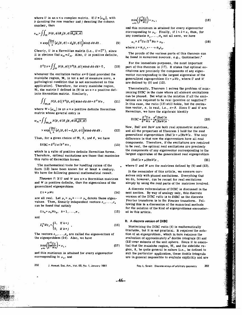
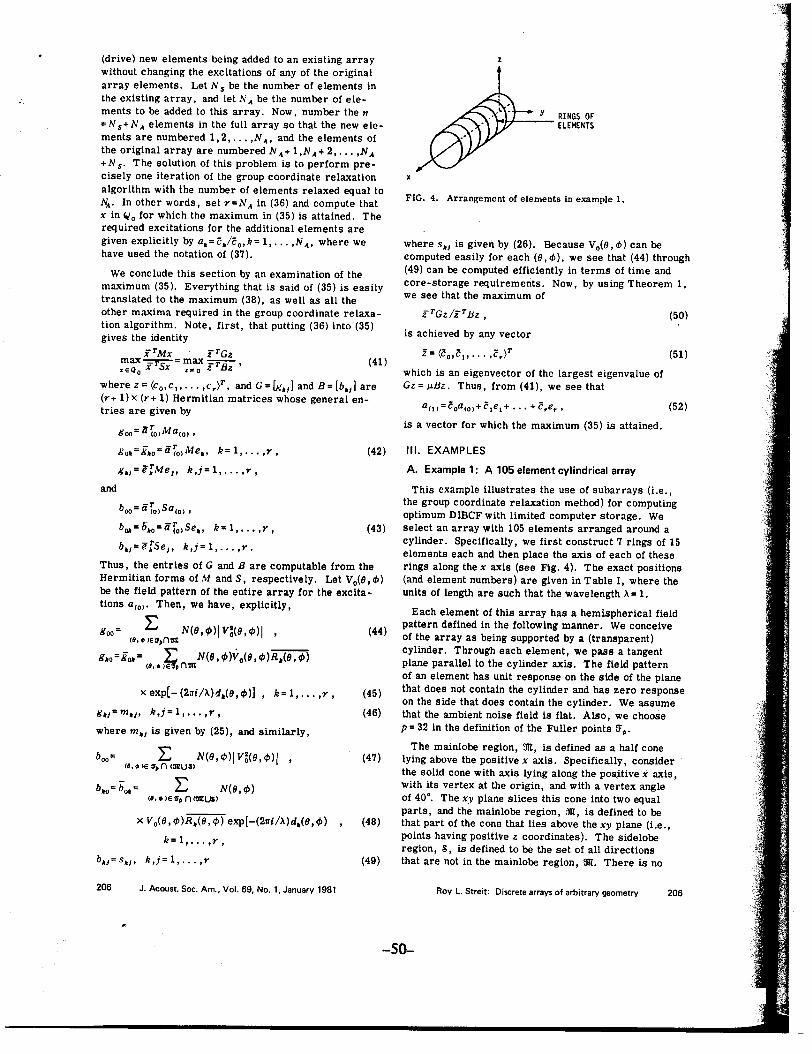
b~~5.0~li;0)Se., k~I,...,r, (43) select an array with 105 elements arranged around a-T . cylinder. Specifically, we first construct 7 rings of 15b.J~ e .Sel' k,) ~ 1,.. . ,r. elements each and then place the axis of each of these

Thus, the entries of G and B are computable from the rings along the x axis (see Fig. 4). The exact positionsHermitian forms of M and S, respectively. Let V 0(9,1/» (and element numbers) are given in Table I, where thebe the field pattern of the entire array for the excita- units of length are such that the wavelength ~ ~ 1.tions a(O)' Then, we have, explicitly, Each element of this array has a hemispherical field

- L 2 pattern defined in the following manner. We conceivegoo- N(9,tp)IVo(9,tp)1 , (44) of the array as being su

p ported by a (transparent)

cB,.'e"n~- ~ . - cylinder. Through each element, we pass a tangentg.0~80.~ "'" N(9,tp)Vo(9,tp)R.(9,tp) Plane Parallel to the Cy linder axis The field Pattern cB,.,e"n~ .

of an element has unit response on the side of the planex ex [- (21Ti/~)d (9 tp)] k~ 1 ... r (45) that doe~ not contain the c~linder an~ has zero responsep .'", , on the slde that does contarn the cyl1nder. We assume

6'.I~ m.J' k,j ~ 1,... ,r, (46) that the ambient noise field is flat. Also, we chooseh .. by (25) nd . .1 1 P ~ 32 in the definition of the Fuller points fJ",.were m.J 1S glven ,a Slm1 ar y,

The mainlobe region, m, is defined as a half coneboo= L N(9, tp)1 V~(9, tp)1 ' (47) lying above the positive x axis. Specifically, consider

(B,. IE', n (~UI) the solid cone with axis lying along the po8-itive i axis,

b ~ b = L N(9 tp) with its vertex at the origin, and with a vertex angle.0 ~ (B,.)E', n c~ua) , of 40°. The xv plane slices this cone into two equal

parts, and the mainlobe region, :JIl, is defined to bex V 0(9, I/»R.(9, 1/» exp[-(21Ti/~)d.(9, tp), (48) that part of the cone that lies above the xy plane (i.e.,

k~ 1 points having positive z coordinates). The sidelobe, . . . , r , region, S, is defined to be the set of all directions

b.J~5.J' k,j~I,...,r (49) thatarenotinthemainloberegion,m. There is no

206 J. Acoust. Soc. Am., Vol. 69, No. I, January 1981 Roy L. Streit: Discrete arrays of arbitrary geometry 206

.,

-SO-

F "

"."c.!

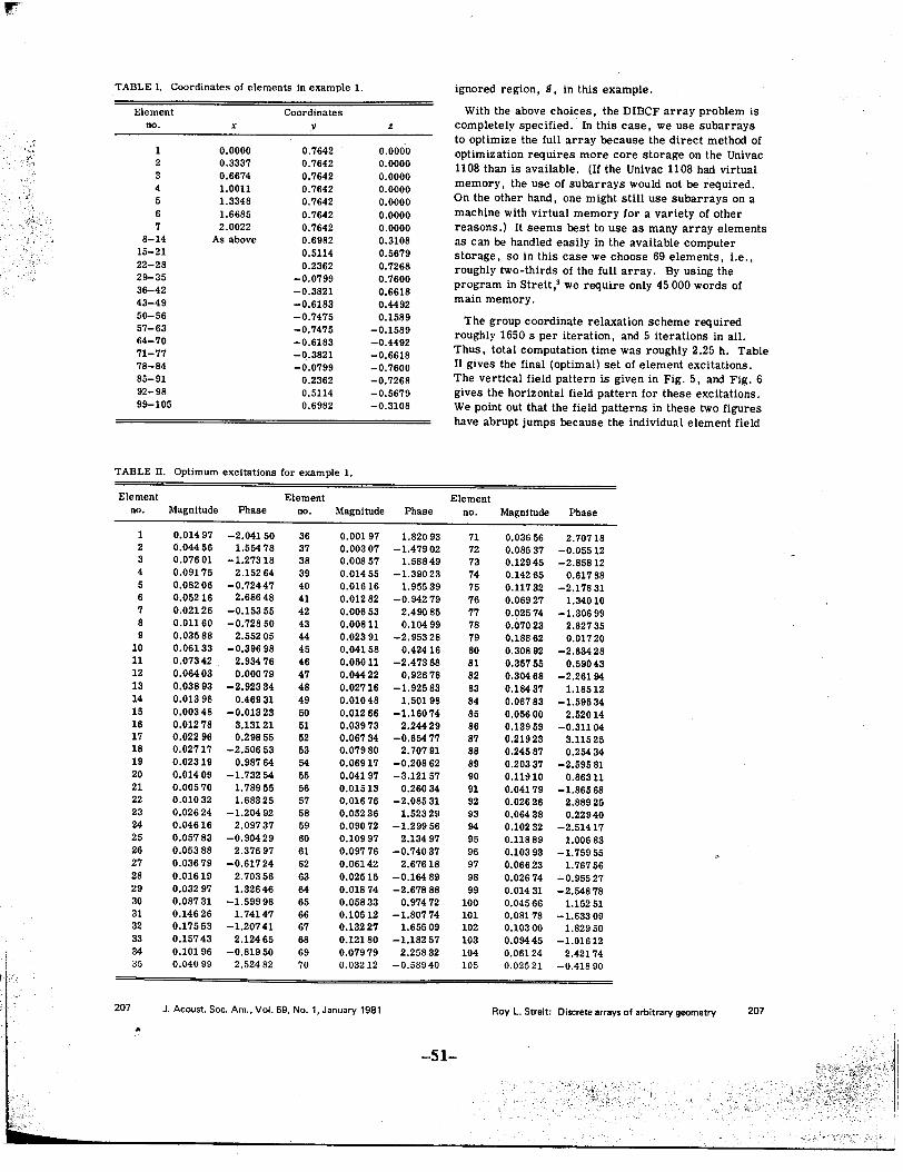
TABLE I. Coordinates of elements in example 1. ignored region, S, in this example.

Element Coordinates With the above choices, the DIBCF array problem isno. x v z completely specified. In this case, we use subarrays

to optimize the full array because the direct method of1 0.0000 0.7642 0.0000 optimization requires more core storage on the Univac2 0.3337 0.7642 0.0000 1108 than is available. (If the Univac 1108 had virtual3 0.6674 0.7642 0.0000 memory, the use of subarrays would not be required.4 1.0011 0.7642 0.0000 . .

11 b5 1.3348 0.7642 0.0000 On the other hand, one might sti use su arrays on a6 1.6685 0.7642 0.0000 machine with virtual memory for a variety of other7 2.0022 0.7642 0.0000 reasons.) It seems best to use as many array elements

8-14 As above 0.6982 0.3108 as can be handled easily in the available computer15-21 0.5114 0.5679 storage, so in this case we choose 69 elements, i.e.,22-28 0.2362 0.7268 roughly two-thirds of the full array. By using the29-35 -0.0799 0.7600 program in Streit 3 we require only 45000 words of36-42 -0.3821 0.6618 . '43-49 -0.6183 0.4492 mam memory.50-56 -0.7475 0.1589 The group coordinate relaxation scheme required57-63 -0.7475 -0.1589 roughly 1650 s per iteration, and 5 iterations in all.64-70 -0.6183 -0.4492 ..

hI 2 25 h T bl71-77 -0 3821 -0.6618 Thus, total computation tlIne was roug y. . a e78-84 -0:0799 -0.7600 II gives the final (optimal) set of element excitations.85-91 0.2362 -0.7268 The vertical field pattern is given in Fig. 5, and Fig. 692-98 0.5114 -0.5679 gives the horizontal field pattern for these excitations.99-105 0.6982 -0.3108 We point out that the field patterns in these two figures

have abrupt jumps because the individual element field

TABLE ll. Optimum excitations for example 1.

Element Element Elementno. Magnitude Phase no. Magnitude Phase no. Magnitude Phase

1 0.01497 -2.04150 36 0.00197 1.82093 71 0.03656 2.707182 0.04456 1.554 78 37 0.00307 -1.47902 72 0.08537 -0.055123 0.07601 -1.27318 38 0.00857 1.58849 73 0.12945 -2.858124 0.09175 2.15264 39 0.01455 -1.39023 74 0.14265 0.617885 0.08206 -0.72447 40 0.01616 1.95539 75 0.11732 -2.178316 0.05216 2.68648 41 0.01282 -0.94279 76 0.06927 1.340107 0.02126 -0.15355 42 0.00653 2.490 85 77 0.02574 -1.306998 0.01160 -0.72850 43 0.00811 0.10499 78 0.07023 2.827359 0.03588 2.55205 44 0.02391 -2.95328 79 0.18862 0.01720

10 0.06133 -0.39698 45 0.04158 0.42416 80 0.30892 -2.8342811 0.07342 2.93476 46 0.05011 -2.47388 81 0.35755 0.5904312 0.06403 0.00079 47 0.04422 0.92678 82 0.304 68 -2.2619413 0.03893 -2.92334 48 0.02716 -1.92583 83 0.18437 1.1851214 0.01398 0.46931 49 0.01048 1.50198 84 0.06783 -1.5953415 0.00348 -0.01323 50 0.01266 -1.16074 85 0.05600 2.5201416 0.01278 3.13121 51 0.03973 2.244 29 86 0.13959 -0.311 0417 0.02296 0.29855 52 0.06734 -0.654 77 87 0.21923 3.1152518 0.02717 -2.50653 53 0.07980 2.70791 88 0.24587 0.254 3419 0.02319 0.98764 54 0.06917 -0.20862 89 0.20337 -2.5958120 0.01409 -1.73254 55 0.04197 -3.12157 90 0.11910 0.8631121 0.00570 1.78955 56 0.01513 0.26034 91 0.04179 -1.8656822 0.01032 1.68325 57 0.01676 -2.08531 92 0.02626 2.8892523 0.02624 -1.20492 58 0.05236 1.52329 93 0.06438 0.2294024 0.04616 2.09737 59 0.09072 -1.29956 94 0.10232 -2.5141725 0.05783 -0.90429 60 0.10997 2.13497 95 0.11889 1.0068326 0.05388 2.37697 61 0.09776 -0.74037 96 0.10393 -1.75955 "27 0.03679 -0.61724 62 0.06142 2.67618 97 0.06623 1.7675628 0.01619 2.70356 63 0.02515 -0.164 89 98 0.02674 -0.9552729 0.03297 1.32646 64 0.01874 -2.67888 99 0.01431 -2.5487830 0.08731 -1.59998 65 0.05833 0.97472 100 0.04566 1.1525131 0.14626 1.74147 66 0.10512 -1.80774 101 0.08178 -1.6330932 0.17553 -1.20741 67 0.13227 1.65509 102 0.10300 1.8295033 0.15743 2.12465 68 0.12180 -1.18257 103 0.094 45 -1.01612

, 34 0.10196 -0.81950 69 0.07979 2.25832 104 0.06124 2.42174! 35 0.04099 2.52482 70 0.03212 -0.58940 105 0.02521 -0.41890

207 J. Acoust. Soc. Am., Vol. 69, No.1, January 1981 Roy L. Streit: Discrete arrays of arbitrary geometry 207

A

-51-

0 T ABLE III. Group coordinate relaxation estimates of largesteigenvalu,,' for examplc 1. -

10 Iteration no. Estimate of largest eigenvalue

~ 20 1 0.91427s: 2 0.96100~ 3 0.96374~ 30 4 0.965328 5 0.96559

CQ 40og

50 B. Example 2: A comparison with Dolph-Chebyshev

60 design-180 -1 - . t .tANGLE MEASUREO FROM x-AXIS (deg) This example serves two purposes. Firs, 1 .pro-

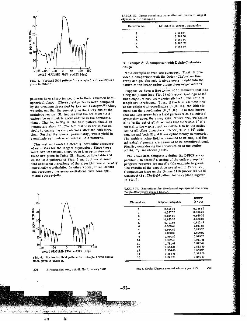
vides a comparison with the Dolph-Chebyshev lineFIG. 5. Vertical field pattern for example 1 with excitations array design. Second, it gives some insight into thegiven in Table I. nature of the lower order eigenvalues/eigenvectors.

Suppose we have a line ar;ay of 15 elements that liesalong the y axis (see Fig. 1) with equal spacings of 0.5

patterns have sharp jumps, due to their assumed hemi- wavelength, where the wavelength x = 1. The units ofspherical shape. (These field patterns were computed length are irrelevant. Thus, if the first element liesby the program described by Lee and Leibiger.'2) Also, at the origin with coordinates (0.,0.,0.), the 15th ele-we point out that the geometry of the array and of the ment has the coordinates (0.,7., 0.). It is well knownmainlobe region, :JR, implies that the optimum field that any line array has a field pattern with cylindricalpattern be symmetric about endfire in the horizontal symmetry about the array axis. Therefore, we defineplane. That is, in Fig. 6, the field pattern should be $ to be the set of all directions that lie within 8° of asymmetric about 0°. The fact that it is not is due en- normal to the y' axis, and we define S to be the collec-tirely to ending the computations after the fifth itera- tion of all other directions. Hence, :JR is a 16° widetion. Further iterations, presumably, would yield in- annulus and both ;J1t and S are cylindrically symmetric.creasingly symmetric horizontal field patterns. The ambient noise field is assumed to be flat, and the

This method creates a steadily increasing sequence individual ele~en~s are assumed t~ be omnidirectional.of estimates for the largest eigenvalue. Since there Finally, considering the construction of the Fullerwere five iterations, there were five estimates and points, fJ" we choose p = 24.

these are given in Table III. Based on this table and The above data completely define the DIBCF arrayon the field patterns of Figs. 5 and 6, it would seem problem. In Streit,3 a listing of the entire computerthat additional iterations of the algorithm would be only program required for exactly this example is given.marginally worthwhile. In other words, to all intents The results of the execution are given in Table IV.and purposes, the array excitations have been opti- Computation time on the Univac 1108 (under EXEC 8)mized successfully. was about 41 s. The field pattern in the xy plane is given

in Fig. 7.

TABLE IV. Excitations for IS-element equlspaced line array:Dolph-Chebyshe!versus DIBCF.

0DIBCF

1 Element no. Dolph-Chebyshev <p = 24)

~ 1 0.34371 0.25687s: 2 0.35775 0.39520~ 3 0.50403 0.54024~ 4 0.65338 0.68290z 5 0.79108 0.81242~ 6 0.90242 0.91188CQ 7 0.97487 0.97920og 8 1.00000 1.00000

9 0.97487 0:9792010 0.90242 0.91188

60 11 0.79108 0.81242-180 -90 0 +90 +180 12 0.65338 0.68290

ANGLE MEASURED FROM x-AXIS (deg) 13 0.50403 0.5402414 0.35775 0.39520

FIG. 6. Horizontal field pattern for example 1 with excita- 15 0.34371 0.25687tions given in Table II.

208 J. Acoust. Soc. Am., Vol. 69, No.1, January 1981 Roy L. Streit: Discrete arrays of arbitrary geometry 208

"

-52-

pI'

0OOLPH-CHEBYSHEV- DIBCF

-10 -1

! -20 i -2

'" ~V' ...Z .~" ~ ,- V'~ -3 I 1/1 I'1I I ~V' I Q. -30'" V'a: '"

I a:

-4

-4

-50-gO - - 0RELATIVE BEARING (deg) -5~gO - -

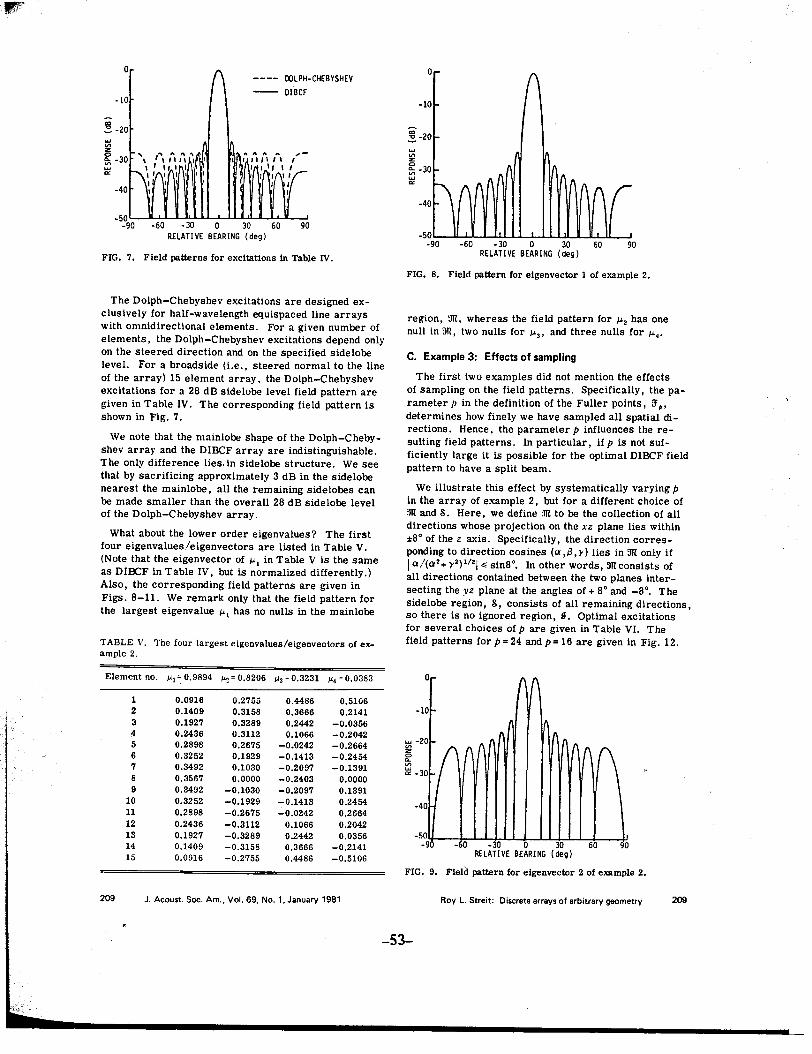
RELATIVE BEARING (deg)FIG. 7. Field patterns for excitations in Table IV.

FIG. B. Field pattern for eigenvector 1 of example 2.

The Dolph-Chebyshev excitations are designed ex-clusively for half-wavelength equispaced line arrays region, ~, whereas the field pattern for 1'"2 has onewith omnidirectional elements. For a given number of null in ~R, two nulls for 1'"3' and three nulls for 1'"..elements, the Dolph-Chebyshev excitations depend onlyon the steered direction and on the specified sidelobe C. Example 3: Effects of samplinglevel. For a broadside (i.e.. steered normal to the line .

I d ' d t t . the effectsThe fIrst two examp es I no men Ionof the array) 15 element array. the Dolph-Chebyshev . .excitations for a 28 dB side lobe level field pattern are of sampling on the fi.el.d.patterns. SpeclfIc~lly, the pa-given in Table IV. The corresponding field pattern is rameter p in the definItIon of the Fuller pOints '. fJ p,.

. F.7 determines how finely we have sampled all spatial dl-

shown In Ig. .

t . fl thrections. Hence. the parame er p In uences e re-We note that the mainlobe shape of the Dolph-Cheby- sulting field patterns. In particular, if p is not suf-

shev array and the DIBCF array are indistinguishable. ficiently large it is possible for the optimal DIBCF fieldThe only difference lies, in sidelobe structure. We see pattern to have a split beam.that by sacrificing approximately 3 dB in the sidelobe . .nearest the mainlobe, all the remaining side lobes can We illustrate this effect by systema!lcally vary~ng pbe made smaller than the overall 28 dB sidelobe level in the array of example. 2. but for a dlfferent.cholCe of

D I h Ch b h ~ and 8. Here, we define ;m to be the collection of allof the op - e ys evarray. " ..directions whose projection on the xz plane lIes wIthin

What about the lower order eigenvalues? The first ,,80 of the z axis. Specifically, the direction corres-four eigenvalues!eigenvectors are listed in Table V. ponding to direction cosines (a,13, Y) lies in ~ only if(Note that the eigenvector of 1'", in Table V is the same I a!(a2+ y2)'/2j.; sin8°. In other words, ~ consists ofas DIBCF in Table IV, but is normalized differently.) all directions contained between the two planes inter-Also, the corresponding field patterns are given in secting the yz plane at the angles of + 80 and -80. TheFigs. 8-11. We remark only that the field pattern for side lobe region, 8, consists of all remaining directions,the largest eigenvalue 1'", has no nulls in the mainlobe so there is no ignored region, S. Optimal excitations

for several choices of p are given in Table VI. Thefield patterns forp=24 andP=16 are given in Fig. 12.TABLE V. The four largest eigenvalues!eigenvectors of ex-

ample 2.

Element no. 111=0.9894 1':!=0.8206 113=0.3231 114=0.0383

1 0.0916 0.2755 0.4486 0.5106i 2 0.1409 0.3158 0.3666 0.2141 -1I 3 0.1927 0.3289 0.2442 -0.0356

4 0.2436 0.3112 0.1066 -0.2042 ... -25 0.2898 0.2675 -0.0242 -0.2664 ~6 0.3252 0.1929 -0.1413 -0.2454 ~7 0.3492 0.1030 -0.2097 -0.1391 ~ -38 0.3567 0.0000 -0.2403 0.00009 0.3492 -0.1030 -0.2097 0.1391

10 0.3252 -0.1929 -0.1413 0.2454 -4011 0.2898 -0.2675 -0.0242 0.266412 0.2436 -0.3112 0.1066 0.204213 0.1927 -0.3289 0.2442 0.0356 -:OgO -60 -30 30 6014 0.1409 -0.3158 0.3666 -0.2141 RELATIVE BEARING (deg)15 0.0916 -0.2755 0.4486 -0.5106

FIG. 9. Field pattern for eigenvector 2 of example 2.

209 J. Acoust. Soc. Am., Vol. 69, No.1, January 1981 RoV L. Streit; Discrete arrays of arbitrary geometry 209

~

-53-

T ABLE VI. Effects of sampling on excitations for example 3.

Element p \-1 no. 16 24 32 40

-;; 1 0.2953 0.1275 0.1322 0.1177::;. -2 2 -0.0064 0.1676 0.1792 0.1662

~ 3 0.3846 0.2207 0.2406 0.2232~ 4 -0.1045 0.2497 0.2613 0.2581~ -30 5 0.2990 0.2884 0.2~46 0.2~340: 6 -0.2830 0.3067 0.2991 0.3099

7 0.1753 0.3337 0.3154 0.3259-4 8 -0.3280 0.3346 0.3117 0.3279

9 0.1753 0.3337 0.3154 0.3259-50 10 -0.2830 0.3067 0.2991 0.3099

-90 - - 11 0.2990 0.2884 0.2946 0.2934RELATIVE BEARING (de9) 12 -0.1045 0.2497 0.2613 0.2581

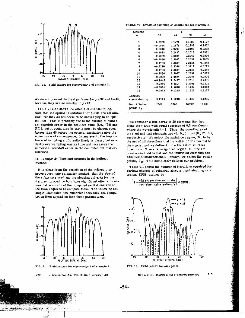
13 03846 0.2207 0.2406 0.2232FIG. 10. Field pattern for eigenvector 3 of example 2. 14 -0:0064 0.1676 0.1792 0.1662

15 0.2953 0.1275 0.1322 0.1177

LargestWe do not present the field patterns for p = 32 and p = 40, eigenvalue, 1'1 0.1149 0.1243 0.1165 0.1225because they are so similar to p = 24. No. of Fuller 2562 5762 10242 16002

Table VI also shows the effects of oversampling. points (;,Note that the optimal excitations for p" 24 are all sim-ilar, but they do not seem to be converging to an opti-mal set. This is probably due to the buildup of numeri- We consider a line array of 25 elements that liescal roundoff error in the required sums [i.e., (25) and along the.v axis with equal spacings of 0.5 wavelength,(26) I, but it could also be that p must be chosen even where the wavelength A = 1. Thus, the coordinates oflarger than 40 before the optimal excitations give the the first and last elements are (0.,0.,0.) and (0.,12.,0.),appearance of convergence. In any event, the impor- respectively. We select the mainlobe region, :Ill, to betance of sampling sufficiently finely is clear, but evi- the set of all directions that lie within 5° of a normal todently oversampling wastes time and increases the the v axis, and we define 8 to be the set of all othernumerical roundoff error in the computed optimal ex- dir~ctions. There is no ignored region, g. The am-citations. bient noise field is flat and the individual elements are

. .. assumed omnidirectional. Finally, we select the FUllerD. Example 4: Time and accuracy In the Indirect

P oints 1F . This completely defines our problem.hod ' 28met .dfTable VII shows the number of iterations require or

It is clear from the definition of the indirect, or various choices of subarray size, n., and stopping cri-group coordinate relaxation method, that the size of terion, EPSI, defined bythe subarrays used and the stopping criteria for the

I

iteration procedure both have significant effects on nu- l1 - old ei.genvalue esti.mate ~ EPSI.merical accuracy of the computed excitations and on I new eigenvalue estimatethe time required to compute them. The following ex-ample illustrates how numerical accuracy and compu-tation time depend on both these parameters.

0 -1

-10 ~

'"

::;'-2~ '"

Ig -20 ~~ 0

~ ~-30Z 0:00. -30VI'"0:

-40-40

-50 -5~90-90 - RELATIVE BEARING (deg) RELATIVE BEARING (deg)

FIG. 11. Field pattern for eigenvector 4 of example 2. FIG. 12. Field pattern for example 3.

210 J. Acoust. Soc. Am.. Vol. 69, No. I, January 1981 Roy L. Streit: Discrete arrays of arbitrary geometry 210

"

-54--

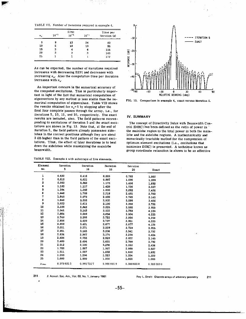
means of computing optimum element excitations for 3R. L. Streit, Array optilnizatton Using Subarrays, NUSC. arrays of arbitrary numbers of elements, yet it re- Technical Report 5889 (Naval Underwater ~ystems Center,

quires only nominal core storage. Conceptually, the , New London, CT, 23 March 1979). .group coordinate relaxation technique employs subar- F. R. Gantmacher, 77le Theory ~f kJatnces (Chelsea. New

h f ' ' t t' York, 1960).ra.ys of t.e ~ll array in a systematIc manner 0 op 1- ~be IMSL Library, Volume 2, International Mathematical andmlZe excltatlons of the full array. Four examples have Statistical Libraries UMSL, Inc., Houston, TX, 1977), 6thbeen included, one of which demonstrates the effec- ed.tiveness of group coordinate relaxation for a cylindrical 6R. S. Martin and J. H. Wilkinson, "Reduction of the symmet-array of 105 elements. ric eigenproblemAx~ABx and relat~d problems to stan-

dard form," Numerische Mathematik 11, 99-110 (1968).ACKNOWLEDGMENTS TD. Slepian and H. O. Pollak, "Prolate spheroidal wave func-

tions, Fourier analysis and uncertainty- I," Bell Syst. Tech.The author would like to thank Mr. Barry G. Buehler J:40, 43-63 (1961).

and Dr. Albert H. Nuttall, both of the New London Lab- 8D. K. Faddeev and Vo N. Faddeeva, Computational Methods oforatory, Naval Underwater Systems Center, for their Linear Algebra (Freeman, San Franci.sco, 1963).

, .. aT. W. Melnyk, O. Knop, and W. R. Smith, "External arrange-helpful comments on the varlOUS drafts of thlS artIcle. t f . t d . t h h Eq ilibri . um. . men s 0 porn s an urn c arges on a sp ere: uMr. Buehler also supplled the author wlth many exam- configurations revisited," Can. J. Chern. 55, 1745-1761pIes using the approach of this article, one of which (1977).is included here as example 1. lOJ. Prenis, "An Introduction to Domes," in The Dome Build-

er's Handbook (Running Press, Philadelphia, 1973).lID. Lee, Maximization of Reverberation Index, NUSC Techni-

cal Report 5375 (Naval Underwater Systems Center, New

IJ. K. Butler and H. Unz, "Beam efficiency and gain optimiza- London, CT, 2 October 1976).tion of antenna arrays with nonuniform spacings," Radio Sci. 12D. Lee and G. A. Leibiger, Computation of Beam Patterns2 (7) (new series), 711-720 (July 1967). and Directivity Indices for Three-Dimensional Arrays with

2J. K. Butler and H. Unz, "Optimization of beam efficiency Arbitrary Element Spacings, NUSC Technical Report 4687and synthesis of nonuniformly spaced arrays," Proc. IEEE (Naval Underwater Systems Center, New London, CT, 22

(Letters) 54, 2007-2008 (December 1966). February 1974).

.

?12 J. Acoust. Soc. Am., Vol. 69, No.1, January 1981 Roy L. Streit: Discrete arrays of arbitrary geometry 212

-56-