Optimization of the AdBlue

evaporation module for

Scania V8 engines

MATTIA ANTONIOTTI

Master of Science Thesis

Stockholm, Sweden 2017

KTH, ROYAL INSTITUTE OF TECHNOLOGY

Optimization of the AdBlue evaporation unit for

Scania V8 engines

Master Thesis in Machine Design, MMK 2017 MKN 201

School of Industrial Engineering and Management

Author :

Mattia Antoniotti

Industrial supervisors :

Mårten Ribbhagen

Rickard Gunsjö

Academic supervisor :

Stefan Björklund

SE-100 44 Stockholm

June 2017

i

Master of Science Thesis MMK 2017: MKN 201

Optimization of the AdBlue evaporation unit for

Scania V8 engines

Mattia Antoniotti

Approved

2017-06-13

Examiner

Ulf Sellgren

Supervisor

Stefan Björklund

Commissioner

Scania CV AB

Contact person

Mårten Ribbhagen

Rickard Gunsjö

Abstract

The aftertreatment techniques introduced to follow the emission legislations require a constant

improvement process to comply with the gradually more stringent demands. SCR is the system used

nowadays to deal with NOx emissions in most heavy-duty vehicles. An aqueous-urea solution, AdBlue,

is sprayed into the evaporation unit, where urea should decompose to ammonia, the reducing agent. This

is a critical step because the NH3 amount available heavily affects the final nitrous oxides reduction to

nitrogen. Moreover the urea decomposition’s sides reactions are likely to occur, forming deposits that

increase the pressure drop and in a certain time period could even foul the system.

The evaporation module used in the silencer for Scania trucks equipped with V8 engines consists of

a pipe in pipe configuration made in stainless steel 1.4509, where the exhaust gases flow heating up the

inner pipe finned on its outer surface. The AdBlue is sprayed on the inner pipe’s inner surface, creating

a wall film and cooling down the tube. The production of the evaporation pipe however involves a costly

manufacturing process, being made of 144 flanges laser welded on a 0.355 m length, for a total of more

than 52 m of welding.

The goal of this thesis is to analyse the heat transfer from the exhaust gases to the pipe and how to

improve it, in order to achieve a lower temperature drop on the pipe due to the AdBlue dosing, reducing

at the same time the risk of building up deposits. The application of different materials for the

evaporation unit is also considered. Furthermore many manufacturing processes are evaluated as a cost-

effective alternative to the current one.

Although the operating points have a wide range of variation, the analysis is focused on the worst

conditions for urea evaporation which are low mass flow and low flow temperature.

Stainless steel is the best trade-off between cost, thermal conductivity and corrosion resistance but

the much higher conductivity of copper alloys would justify the investigation of a copper evaporation

pipe coated with stainless steel.

Different designs of the heat flanges are assessed, first with correlations and FEA and then through

a CFD analysis, where 62 different solutions are compared. The fins height results to be the most

influencing parameter, requiring an increment from 7.5 mm to 11 mm to improve the heat transfer

performances of the evaporation unit. The gap between each fin is also important, leading to a flanges

quantity reduction suggestion. With the current fin design and half of the number of flanges, 11 mm

high, the performances would improve by almost 40% (at 800 kg/h and 300 ℃). Furthermore both the

Abstract

ii

pipe thickness and thermal conductivity are affecting the temperature drop, with different weight

depending on the design and the operating point. It is however always advantageous to use a thicker

wall and a material with a higher thermal conductivity.

Lastly the tests performed on the specifically developed test rig show a good accordance with the

simulations in comparing different materials but are not suitable to compare finned designs.

Keywords: SCR, evaporation unit, urea deposits, heat fins

iii

Examensarbete MMK 2017: MKN 201

Optimering av AdBlue-förångningsmodulen för Scania V8-motorer

Mattia Antoniotti

Godkänt

2017-06-13

Examinator

Ulf Sellgren

Handledare

Stefan Björklund

Uppdragsgivare

Scania CV AB

Kontaktperson

Mårten Ribbhagen

Rickard Gunsjö

Sammanfattning

Avgasefterbehandlingssystem har utvecklats för att reducera utsläppen ifrån lastbilar, och det är ett

lagkrav att en lastbil ska ha ett efterbehandlingssystem. Lagkraven för avgasemissioner skärps gradvis,

vilket resulterar i att efterbehandlingssystemet ständigt måste förbättras och utvecklas för att möta de

nya lagkraven.

I de flesta heavy-duty-lastbilar som säljs på Euro 6 marknader är ett SCR-system installerat ihop med

ljuddämparen för att hantera NOx-utsläppen. En vätska kallad AdBlue, det vill säga Urea, sprayas in i

efterbehandlingssystemet där det förångas. Urea är en vätska baserad på bl.a. urinämne som utsöndras

till ammoniak, vilket sedan fungerar som reduceringsmedel.

Ett viktigt steg i reduktionsprocessen av kväveoxiden är när ammoniak reagerar med NOx och

omvandlas till kväve och vatten. Det är mängden ammoniak som bestämmer det slutliga resultatet av

kväveoxidreduktionen. Om urean inte är tillräckligt uppblandad med avgaserna bildas avlagringar

utmed flödeskanalen. Detta ökar tryckfallet, vilket i sin tur leder till ökad bränsleförbrukning,

avlagringarna kan över tid även skada efterbehandlingssystemet.

Förångningsmodulen som används i Scanias ljuddämpare (kallad large), utvecklad för V8-motorer,

består av en rör-i-rör konfiguration. Rören tillverkas i rostfritt stål 1.4509 och när AdBlue sprayas på

insidan av innerröret bildas en film av urea som förångas när den möter rörets varma väggyta. För att

uppnå en varm förångningsyta leds en delmängd av avgaserna om på utsidan av innerröret för att

bibehålla hög temperatur på röret och undvika nedkylning av urean.

Förångningsrörets nuvarande design består av 144 utvändiga värmeflänsar (med längden 0,355 m)

som lasersvetsas fast på röret. Designen medför en dyr och komplicerad tillverkningsprocess. Den totala

längden svets uppgår till 52 m.

Syftet med examensarbetet är att analysera och förbättra värmeöverföringen från avgaserna till röret

för largeljuddämparen. En förbättrad värmeöverföring skulle leda till att temperaturfallet som

uppkommer på grund av AdBlue-doseringen blir lägre. Ett lägre temperaturfall skulle då leda till en

minskad risk för avlagringar. I studien undersöks olika material och tillverkningsmetoder för att

eventuellt reducera tillverkningskostnaden av förångningsenheten med bibehållen eller förbättrad

prestanda. Driftfallen har ett brett spektrum där mängden energi (överförd värme) varierar och studien

är inriktad på de värsta förhållandena för urea-utsöndring, dvs. ett lågt massflöde och låga

flödestemperaturer.

Sammanfattning

iv

Rostfritt stål har bra korrosionsbeständighet och tämligen bra värmeledningsförmåga i kombination

med ett rimligt pris. Kopparlegeringar har en mycket högre värmeledningsförmåga än rostfritt stål, vilket

motiverar en undersökning av förångringsrör tillverkade i kopparlegering belagda med rostfritt stål.

I studien undersöks olika utformning av värmeflänsar, både genom FEA och CFD-analyser, där 62

olika utformningar har tagits fram och jämförs. Flänsarnas höjd visade sig vara den parametern som

påverkar temperaturfallet mest. En ökning från 7,5 mm till 11 mm av flänstoppens höjd gav en kraftig

förbättring av förångningsenhetens värmeöverföringsförmåga. En annan viktig faktor visade sig vara

avståndet mellan flänsarna. Med dagens flänsutformning, men med en utökad höjd till 11 mm, skulle

man uppnå en förbättrad prestanda med nästan 40 % (vid 300℃ och 800 kg/h) om man dessutom

minskade antalet flänsar med hälften. Beroende på design och driftspunkt är rörtjockleken och

materialets värmeledningsförmåga andra faktorer som påverkar temperaturfallet. Det är dock oftast

fördelaktigt med en tjockare rörvägg och ett material med högre värmeledningsförmåga.

Flera prototyper med olika utformning har testats fysiskt i en specialtillverkad testrigg. Slutresultatet

påvisade en bra korrelation med simuleringarna vid jämförelse av olika materialval, men det fysiska

testet hade svårare att hantera geometrisk utformning på flänsarna.

Nyckelord: Urea, förångningsmodulen, ureaavlagringar, rörflänsar

v

Contents

Abstract................................................................................................................................... i

Sammanfattning .................................................................................................................... iii

Contents ................................................................................................................................. v

List of Figures ..................................................................................................................... viii

List of Tables ........................................................................................................................ xii

Notations ............................................................................................................................. xiii

Acknowledgments .................................................................................................................xv

1. Introduction ................................................................................................................. 1

1.1. Diesel combustion ...................................................................................................... 1

1.2. Pollutants ................................................................................................................... 4

1.2.1. NOx .................................................................................................................... 4

1.2.2. PM ..................................................................................................................... 4

1.2.3. HC ..................................................................................................................... 5

1.2.4. CO ..................................................................................................................... 5

1.3. Diesel Oxidation Catalyst ............................................................................................ 5

1.4. Methods of reducing NOx............................................................................................ 6

1.4.1. EGR ................................................................................................................... 6

1.4.2. LNTs (Lean NOx traps) ........................................................................................ 7

1.4.3. In cylinder control ............................................................................................... 8

1.5. SCR........................................................................................................................... 8

1.6. AdBlue chemistry ......................................................................................................10

1.6.1. Urea ..................................................................................................................11

1.6.2. NH3 ...................................................................................................................13

1.7. Problem description ...................................................................................................14

1.7.1. Urea deposit formation .......................................................................................15

1.7.2. Methodology......................................................................................................16

1.8. Scania silencers family...............................................................................................17

2. Heat Transfer Analysis ................................................................................................19

2.1. Heat transfer theory ...................................................................................................19

2.1.1. Conduction ........................................................................................................19

2.1.2. Convection.........................................................................................................20

2.1.3. Irradiation ..........................................................................................................20

2.1.4. Conduction equation ...........................................................................................21

Contents

vi

2.2. Heat transfer calculations ...........................................................................................23

2.2.1. Convection correlations ......................................................................................23

2.2.2. Friction factor and Pressure losses .......................................................................25

2.2.3. Hypotesis ...........................................................................................................27

2.2.4. Fins study ..........................................................................................................29

2.2.5. Results...............................................................................................................39

2.2.6. Other possible interpretation ...............................................................................43

2.3. FEM analysis ............................................................................................................45

2.3.1. Results...............................................................................................................49

2.3.2. Summary and discussions ...................................................................................54

3. Materials for exhaust systems ......................................................................................57

3.1. Corrosion ..................................................................................................................57

3.1.1. Carburization and nitridation ...............................................................................57

3.1.2. Oxidation ...........................................................................................................57

3.1.3. Sulphidation and attack by halogen gases .............................................................58

3.2. Stainless Steels ..........................................................................................................58

3.2.1. Ferritic stainless steels ........................................................................................59

3.2.2. Austenitic stainless steels ....................................................................................60

3.2.3. Martensitic stainless steels ..................................................................................60

3.2.4. Duplex stainless steels ........................................................................................60

3.2.5. Precipitation Hardened stainless steels .................................................................61

3.3. Stainless steels for evaporator pipe..............................................................................61

3.4. Alternative materials ..................................................................................................65

3.4.1. Cu-Cr-Zr alloy ...................................................................................................67

3.4.2. Chromium..........................................................................................................70

3.4.3. Nickel................................................................................................................71

3.4.4. Others................................................................................................................71

3.5. Summary ..................................................................................................................71

4. Manufacturing processes .............................................................................................73

4.1. Manufacturing processes used for Scania’s evaporation units .......................................73

4.1.1. Large silencer.....................................................................................................73

4.1.2. Medium silencer.................................................................................................73

4.1.3. Common silencer ...............................................................................................74

4.2. Forming ....................................................................................................................74

4.2.1. Stresses analysis .................................................................................................75

4.2.2. Formability ........................................................................................................78

4.2.3. Materials in forming ...........................................................................................78

Contents

vii

4.2.4. Hot forming .......................................................................................................81

4.3. Extrusion ..................................................................................................................82

4.3.1. Economic investigation.......................................................................................84

4.4. Cold forming pipe’s manufacturing.............................................................................86

4.5. Casting .....................................................................................................................87

4.6. Machining .................................................................................................................90

4.7. Further possible techniques ........................................................................................92

4.8. Summary ..................................................................................................................96

5. CFD simulations ..........................................................................................................99

5.1. Equations governing CFD ..........................................................................................99

5.2. Concept behind the simulations ................................................................................ 100

5.3. Parameters of DOE .................................................................................................. 100

5.4. Simplifications and boundary conditions ................................................................... 103

5.5. Results .................................................................................................................... 105

5.6. Summary and discussions......................................................................................... 109

6. Tests .......................................................................................................................... 111

6.1. Test rig ................................................................................................................... 111

6.2. Specimen ................................................................................................................ 112

6.3. Temperature sensors and positioning......................................................................... 113

6.4. Design of experiments ............................................................................................. 115

6.5. Test cell system ....................................................................................................... 116

6.6. The dosing unit........................................................................................................ 118

6.7. Test procedure ......................................................................................................... 119

6.8. Performance evaluation............................................................................................ 121

6.9. Results .................................................................................................................... 122

7. Conclusions ............................................................................................................... 127

7.1. Recommendations for future work ............................................................................ 128

Appendix A : Air Properties ................................................................................................ 129

Appendix B : Reynolds and friction factor for the different designs .................................... 130

Appendix C : Stainless steels compositions .......................................................................... 136

Appendix D : Tested designs drawings ................................................................................ 140

Appendix E : Recommended models ................................................................................... 143

References ........................................................................................................................... 145

viii

List of Figures

Figure 1.1. Diffusion flame structure . . . . . . . . . . . . . . . . . . . . . . . . . . . . . . . . . . . . . . . . . . . 1

Figure 1.2. Flame regions detail . . . . . . . . . . . . . . . . . . . . . . . . . . . . . . . . . . . . . . . . . . . . . . . 2

Figure 1.3. Combustion in a diesel engine . . . . . . . . . . . . . . . . . . . . . . . . . . . . . . . . . . . . . . . 2

Figure 1.4. Evolution of emissions legislation for heavy duty (left) and light-duty (right)

diesel vehicles in EU . . . . . . . . . . . . . . . . . . . . . . . . . . . . . . . . . . . . . . . . . . . . . .

3

Figure 1.5. Typical composition of particulate matter emitted from heavy-duty diesel

engine operating under the test cycle . . . . . . . . . . . . . . . . . . . . . . . . . . . . . . . . .

4

Figure 1.6. Three-way catalyst conversion efficiency . . . . . . . . . . . . . . . . . . . . . . . . . . . . . 6

Figure 1.7. EGR concept . . . . . . . . . . . . . . . . . . . . . . . . . . . . . . . . . . . . . . . . . . . . . . . . . . . 7

Figure 1.8. Relation between oxygen content, peak temperature and NOx production . . . . 7

Figure 1.9. SCR system . . . . . . . . . . . . . . . . . . . . . . . . . . . . . . . . . . . . . . . . . . . . . . . . . . . . . 9

Figure 1.10. Example of a complete aftertreatment system . . . . . . . . . . . . . . . . . . . . . . . . . . 10

Figure 1.11. Urea chemical structure . . . . . . . . . . . . . . . . . . . . . . . . . . . . . . . . . . . . . . . . . . . 11

Figure 1.12. Urea decomposition trend . . . . . . . . . . . . . . . . . . . . . . . . . . . . . . . . . . . . . . . . . . 12

Figure 1.13. Urea by-products morphology . . . . . . . . . . . . . . . . . . . . . . . . . . . . . . . . . . . . . . 13

Figure 1.14. Ammonia chemical structure . . . . . . . . . . . . . . . . . . . . . . . . . . . . . . . . . . . . . . . 13

Figure 1.15. Silencer assembly 3D section with component detail . . . . . . . . . . . . . . . . . . . . . 14

Figure 1.16. Fins detail . . . . . . . . . . . . . . . . . . . . . . . . . . . . . . . . . . . . . . . . . . . . . . . . . . . . . . . 15

Figure 1.17. Deposits behaviour with a variable temperature . . . . . . . . . . . . . . . . . . . . . . . . . . 15

Figure 1.18. Deposit formation on a hot plate . . . . . . . . . . . . . . . . . . . . . . . . . . . . . . . . . . . . . 16

Figure 1.19. Medium silencer section . . . . . . . . . . . . . . . . . . . . . . . . . . . . . . . . . . . . . . . . . . . 18

Figure 2.1. Similar configuration of the evaporation module . . . . . . . . . . . . . . . . . . . . . . . . 23

Figure 2.2. Moody chart . . . . . . . . . . . . . . . . . . . . . . . . . . . . . . . . . . . . . . . . . . . . . . . . . . . . 26

Figure 2.3. Evaporation unit section . . . . . . . . . . . . . . . . . . . . . . . . . . . . . . . . . . . . . . . . . . . 27

Figure 2.4. Five different designs analysed in this first phase, a) SRL, b) STL, c) current

design, d) SRR and e) U shape design . . . . . . . . . . . . . . . . . . . . . . . . . . . . . . . .

28

Figure 2.5. Example of a thermal equivalent for a case like the one treated here, but with

opposite cold and hot sides . . . . . . . . . . . . . . . . . . . . . . . . . . . . . . . . . . . . . . . . .

29

Figure 2.6. Dimensions and coordinates of a longitudinal fin of rectangular shape with tip

heat loss . . . . . . . . . . . . . . . . . . . . . . . . . . . . . . . . . . . . . . . . . . . . . . . . . . . . . . . .

32

Figure 2.7. Harper-Brown approximation dimensions . . . . . . . . . . . . . . . . . . . . . . . . . . . . . 32

Figure 2.8. Triangular fin dimensions and coordinates . . . . . . . . . . . . . . . . . . . . . . . . . . . . . 33

Figure 2.9. Gardner's graph for longitudinal fin efficiencies . . . . . . . . . . . . . . . . . . . . . . . . 34

Figure 2.10. Draft of the electrical equivalence for the current design . . . . . . . . . . . . . . . . . . 35

Figure 2.11. Electrical equivalent for heat transfer . . . . . . . . . . . . . . . . . . . . . . . . . . . . . . . . . 36

Figure 2.12. Helical fins draft and dimensions . . . . . . . . . . . . . . . . . . . . . . . . . . . . . . . . . . . . 37

Figure 2.13. UA plotted as a function of fins height and number, for SRL fins . . . . . . . . . . . 39

Figure 2.14. UA plotted as a function of fins height and number, for STL fins . . . . . . . . . . . 40

Figure 2.15. Rectangular UA plot with copper material instead . . . . . . . . . . . . . . . . . . . . . . . 40

Figure 2.16. UA plotted as a function of fins height and number, for the current design . . . . 41

Figure 2.17. UA plotted as a function of fins height and number, for the U shape design . . . . . 42

List of Figures

ix

Figure 2.18. UA plotted as a function of fins height and number, for SRL fins, with

mixer . . . . . . . . . . . . . . . . . . . . . . . . . . . . . . . . . . . . . . . . . . . . . . . . . . . . . . . . . .

43

Figure 2.19. 2D fem analysis example . . . . . . . . . . . . . . . . . . . . . . . . . . . . . . . . . . . . . . . . . . 45

Figure 2.20. Loading “areas”. White : minimum, red : maximum, green : average . . . . . . . . . 46

Figure 2.21. Short load condition . . . . . . . . . . . . . . . . . . . . . . . . . . . . . . . . . . . . . . . . . . . . . . 47

Figure 2.22. Long load condition . . . . . . . . . . . . . . . . . . . . . . . . . . . . . . . . . . . . . . . . . . . . . . 47

Figure 2.23. Example of the temperature distribution resulting from a long load, with 350 ℃ and 450 𝑘𝑔/ℎ on a SRL design . . . . . . . . . . . . . . . . . . . . . . . . . . . . . . . . . . . . .

48

Figure 2.24. Example of the temperature distribution resulting from a short load, with 350 ℃ and 450 𝑘𝑔/ℎ on a SRL design . . . . . . . . . . . . . . . . . . . . . . . . . . . . . . . . . . . . .

48

Figure 2.25. Performance comparison of different solutions, with long load, 200 ℃ and 450𝑘𝑔/ℎ . . . . . . . . . . . . . . . . . . . . . . . . . . . . . . . . . . . . . . . . . . . . . . . . . . . . . . .

49

Figure 2.26. Performance comparison of different solutions, with short load, 200 ℃ and 450𝑘𝑔/ℎ . . . . . . . . . . . . . . . . . . . . . . . . . . . . . . . . . . . . . . . . . . . . . . . . . . . . . . .

50

Figure 2.27. Performance comparison of different solutions, with long load, 350 ℃ and 450𝑘𝑔/ℎ . . . . . . . . . . . . . . . . . . . . . . . . . . . . . . . . . . . . . . . . . . . . . . . . . . . . . . .

50

Figure 2.28. Performance comparison of different solutions, with short load, 350 ℃ and 450𝑘𝑔/ℎ . . . . . . . . . . . . . . . . . . . . . . . . . . . . . . . . . . . . . . . . . . . . . . . . . . . . . . .

51

Figure 2.29. Performance comparison of different solutions, with long load, 300 ℃ and

800𝑘𝑔/ℎ . . . . . . . . . . . . . . . . . . . . . . . . . . . . . . . . . . . . . . . . . . . . . . . . . . . . . . .

51

Figure 2.30. Performance comparison of different solutions, with short load, 300 ℃ and

800𝑘𝑔/ℎ . . . . . . . . . . . . . . . . . . . . . . . . . . . . . . . . . . . . . . . . . . . . . . . . . . . . . . .

52

Figure 2.31. Performance comparison of different solutions, with long load, 200 ℃ and

1850𝑘𝑔/ℎ . . . . . . . . . . . . . . . . . . . . . . . . . . . . . . . . . . . . . . . . . . . . . . . . . . . . . .

52

Figure 2.32. Pipe detail with mixer (in violet) . . . . . . . . . . . . . . . . . . . . . . . . . . . . . . . . . . . . . 53

Figure 2.33. Performance comparison of different solutions, with long load, 200 ℃ and 450𝑘𝑔/ℎ, considering the mixer presence . . . . . . . . . . . . . . . . . . . . . . . . . . . . .

54

Figure 2.34. Performance comparison of different solutions, with short load, 200 ℃ and 450𝑘𝑔/ℎ, considering the mixer presence . . . . . . . . . . . . . . . . . . . . . . . . . . . . .

54

Figure 3.1. Schaeffler-Delong Diagram . . . . . . . . . . . . . . . . . . . . . . . . . . . . . . . . . . . . . . . . 59

Figure 3.2. Ferritic cell . . . . . . . . . . . . . . . . . . . . . . . . . . . . . . . . . . . . . . . . . . . . . . . . . . . . . 59

Figure 3.3. Austenitic cell . . . . . . . . . . . . . . . . . . . . . . . . . . . . . . . . . . . . . . . . . . . . . . . . . . . 60

Figure 3.4. Results from the R. Floyd et al. tests at 300 ℃ . . . . . . . . . . . . . . . . . . . . . . . . . . 62

Figure 3.5. Results from the R. Floyd et al. tests at 500 ℃ . . . . . . . . . . . . . . . . . . . . . . . . . . 62

Figure 3.6. Results from the R. Floyd et al. tests at 650 ℃ . . . . . . . . . . . . . . . . . . . . . . . . . . 63

Figure 3.7. Total penetration of nitriding corrosion attack on laboratory simulation bench

after 300h test (fast heat cycle) done by S. Saedlou and P. Santacreu [8] . . . . . . .

63

Figure 3.8. Influence of chloride pollutant on corrosion by urea decomposition products

(fast heat cycle) from S. Saedlou and P. Santacreu’s study [8] . . . . . . . . . . . . . . .

64

Figure 3.9. Thermal conductivity vs Price for all stainless steel materials . . . . . . . . . . . . . . . 64

Figure 3.10. Thermal conductivity vs Price for all materials commercially available . . . . . . . . 65

Figure 3.11. Thermal conductivity vs Price for all metals . . . . . . . . . . . . . . . . . . . . . . . . . . . . . 66

Figure 3.12. Creep rates function of the applied stress for some copper alloys . . . . . . . . . . . . . 67

Figure 3.13. Strain trend with time for copper alloys exposed to a certain stress . . . . . . . . . . . . 68

Figure 3.14. Thermal conductivity as a function of temperature . . . . . . . . . . . . . . . . . . . . . . . . 68

List of Figures

x

Figure 3.15. Yield strength decrease with temperature . . . . . . . . . . . . . . . . . . . . . . . . . . . . . . 69

Figure 3.16. Galvanic potential series in seawater . . . . . . . . . . . . . . . . . . . . . . . . . . . . . . . . . 70

Figure 4.1. Stress-strain curve using the data from table 1 for different materials . . . . . . . . . 76

Figure 4.2. Graphical representation of the values from table 4.5 for copper alloys (blue

line) and stainless steels (red line) . . . . . . . . . . . . . . . . . . . . . . . . . . . . . . . . . . . .

77

Figure 4.3. Experimental curves with different strain rates 휀1̇ < 휀2̇ < 휀3̇ < 휀4̇ . . . . . . . . . . . 77

Figure 4.4. Effect of stress state on formability [30] . . . . . . . . . . . . . . . . . . . . . . . . . . . . . . . 78

Figure 4.5. Mechanical properties (Rm, Rp02 and A) change with elongation for electrolyte

copper [31, 32] . . . . . . . . . . . . . . . . . . . . . . . . . . . . . . . . . . . . . . . . . . . . . . . . . .

79

Figure 4.6. Flow stress vs True strain for three different steels [29] . . . . . . . . . . . . . . . . . . . . 80

Figure 4.7. Hardness increase during cold forming of different materials [33] . . . . . . . . . . . . 80

Figure 4.8. Direct and indirect extrusion (left) and hydrostatic extrusion (right) . . . . . . . . . . 82

Figure 4.9. Force trend function of ram displacement with different types of extrusion . . . . . 82

Figure 4.10. Manufacturing methods achievable accuracy . . . . . . . . . . . . . . . . . . . . . . . . . . . . 83

Figure 4.11. Comparison between machining and forming in manufacturing costs for a

simple component [36] . . . . . . . . . . . . . . . . . . . . . . . . . . . . . . . . . . . . . . . . . . . .

85

Figure 4.12. Casting methods overview . . . . . . . . . . . . . . . . . . . . . . . . . . . . . . . . . . . . . . . . . 87

Figure 4.13. Skiving process for a heat sink plate . . . . . . . . . . . . . . . . . . . . . . . . . . . . . . . . . . 91

Figure 5.1. Simple scheme of the parameters . . . . . . . . . . . . . . . . . . . . . . . . . . . . . . . . . . . . 101

Figure 5.2. Boundary conditions . . . . . . . . . . . . . . . . . . . . . . . . . . . . . . . . . . . . . . . . . . . . . . 104

Figure 5.3. Minimum temperature in the solid vs pressure drop . . . . . . . . . . . . . . . . . . . . . 105

Figure 5.4. Temperature drop vs fins number . . . . . . . . . . . . . . . . . . . . . . . . . . . . . . . . . . . . 106

Figure 5.5. Temperature drop vs fins height . . . . . . . . . . . . . . . . . . . . . . . . . . . . . . . . . . . . . 107

Figure 5.6. Temperature drop vs fins width . . . . . . . . . . . . . . . . . . . . . . . . . . . . . . . . . . . . . 107

Figure 5.7. Temperature drop vs fins gap . . . . . . . . . . . . . . . . . . . . . . . . . . . . . . . . . . . . . . . 108

Figure 5.8. Temperature drop vs pipe weight . . . . . . . . . . . . . . . . . . . . . . . . . . . . . . . . . . . . 108

Figure 6.1. Previously available test rig . . . . . . . . . . . . . . . . . . . . . . . . . . . . . . . . . . . . . . . . 111

Figure 6.2. Updated test rig section . . . . . . . . . . . . . . . . . . . . . . . . . . . . . . . . . . . . . . . . . . . . 112

Figure 6.3. Test plate . . . . . . . . . . . . . . . . . . . . . . . . . . . . . . . . . . . . . . . . . . . . . . . . . . . . . . . 113

Figure 6.4. Spacing sleeve dimensions . . . . . . . . . . . . . . . . . . . . . . . . . . . . . . . . . . . . . . . . . 113

Figure 6.5. Test plate with sensors positioning . . . . . . . . . . . . . . . . . . . . . . . . . . . . . . . . . . . 113

Figure 6.6. Test plate with sensors . . . . . . . . . . . . . . . . . . . . . . . . . . . . . . . . . . . . . . . . . . . . 114

Figure 6.7. Thermocouple sensor used (the measuring junction is separated to show the two

wires) . . . . . . . . . . . . . . . . . . . . . . . . . . . . . . . . . . . . . . . . . . . . . . . . . . . . . . . . . .

114

Figure 6.8. Circuit of a type K thermocouple . . . . . . . . . . . . . . . . . . . . . . . . . . . . . . . . . . . . . 115

Figure 6.9. Test rig system during an automated test . . . . . . . . . . . . . . . . . . . . . . . . . . . . . . . 116

Figure 6.10. Heating system . . . . . . . . . . . . . . . . . . . . . . . . . . . . . . . . . . . . . . . . . . . . . . . . . . 117

Figure 6.11. AR1 test cell control station. . . . . . . . . . . . . . . . . . . . . . . . . . . . . . . . . . . . . . . . . 117

Figure 6.12. Test rig with components . . . . . . . . . . . . . . . . . . . . . . . . . . . . . . . . . . . . . . . . . . . 118

Figure 6.13. Dosing unit used for the tests . . . . . . . . . . . . . . . . . . . . . . . . . . . . . . . . . . . . . . . . 118

Figure 6.14. Example of a test performed on a FSS 1.25 mm thick simple plate . . . . . . . . . . 119

Figure 6.15. AdBlue dosing, flow temperature and mass flow during the test . . . . . . . . . . . . . 120

Figure 6.16. Example of a long test cycle . . . . . . . . . . . . . . . . . . . . . . . . . . . . . . . . . . . . . . . . . 121

List of Figures

xi

Figure 6.17. Parameters of the long test cycle . . . . . . . . . . . . . . . . . . . . . . . . . . . . . . . . . . . . . 121

Figure 6.18. Performance coefficient in terms of minimum temperatures . . . . . . . . . . . . . . . . 123

Figure 6.19. Performance coefficient in terms of temperature drops . . . . . . . . . . . . . . . . . . . . 123

Figure 6.20. Transients time needed to reach the steady state condition after starting dosing at 450 𝑘𝑔/ℎ and 200 ℃ . . . . . . . . . . . . . . . . . . . . . . . . . . . . . . . . . . . . . . . . . . .

124

Figure 6.21. Deposits witnessing urea flow backwards between the fins . . . . . . . . . . . . . . . . 125

Figure 8.1. Reynolds number in the annulus, for SRL fins . . . . . . . . . . . . . . . . . . . . . . . . . . 130

Figure 8.2. Reynolds number in the inner pipe, for SRL fins . . . . . . . . . . . . . . . . . . . . . . . . . 130

Figure 8.3. Friction factor in the annulus, for SRL fins . . . . . . . . . . . . . . . . . . . . . . . . . . . . . 131

Figure 8.4. Reynolds number in the annulus, for STL fins . . . . . . . . . . . . . . . . . . . . . . . . . . . 131

Figure 8.5. Reynolds number in the inner pipe, for STL fins . . . . . . . . . . . . . . . . . . . . . . . . . 132

Figure 8.6. Friction factor in the annulus, for SRL fins . . . . . . . . . . . . . . . . . . . . . . . . . . . . . 132

Figure 8.7. Reynolds number in the annulus, for current fins . . . . . . . . . . . . . . . . . . . . . . . . . 133

Figure 8.8. Reynolds number in the inner pipe, for current fins . . . . . . . . . . . . . . . . . . . . . . . 133

Figure 8.9. Friction factor in the annulus, for current fins . . . . . . . . . . . . . . . . . . . . . . . . . . . . 134

Figure 8.10. Reynolds number in the annulus, for U shape fins . . . . . . . . . . . . . . . . . . . . . . . . 134

Figure 8.11. Reynolds number in the inner pipe, for U shape fins . . . . . . . . . . . . . . . . . . . . . . 135

Figure 8.12. Friction factor in the annulus, for U shape fins . . . . . . . . . . . . . . . . . . . . . . . . . . 135

Figure 8.13. Current design, cut and flattened from an already existing pipe . . . . . . . . . . . . . 140

Figure 8.14. Simple pipe design (1,25 mm and 3 mm) made of ferritic stainless steel . . . . . . 140

Figure 8.15. Simple pipe designs made of copper (change) . . . . . . . . . . . . . . . . . . . . . . . . . . . 141

Figure 8.16. Simple pipe design made of austenitic stainless steel . . . . . . . . . . . . . . . . . . . . . . 141

Figure 8.17. Design #12 in ferritic stainless steel . . . . . . . . . . . . . . . . . . . . . . . . . . . . . . . . . . 142

Figure 8.18. Current design final recommendation . . . . . . . . . . . . . . . . . . . . . . . . . . . . . . . . . . 143

Figure 8.19. U shape design final recommendation . . . . . . . . . . . . . . . . . . . . . . . . . . . . . . . . . 144

xii

List of Tables

Table 1.1. Euro 5 and 6 limits for heavy-duty Diesel engines . . . . . . . . . . . . . . . . . . . . . . . . 3

Table 1.2. Common SCR reactions . . . . . . . . . . . . . . . . . . . . . . . . . . . . . . . . . . . . . . . . . . . . . . . 9

Table 2.1. Average roughness values for commercial pipe materials [5] . . . . . . . . . . . . . . . . 25

Table 2.2. Critical heights . . . . . . . . . . . . . . . . . . . . . . . . . . . . . . . . . . . . . . . . . . . . . . . . . . . . 42

Table 2.3. Material properties used in the FEM analysis . . . . . . . . . . . . . . . . . . . . . . . . . . . . 46

Table 3.1. SS EN 1.4509 composition . . . . . . . . . . . . . . . . . . . . . . . . . . . . . . . . . . . . . . . . . . . . 61

Table 3.2. SS EN 1.4509 Physical properties [18] . . . . . . . . . . . . . . . . . . . . . . . . . . . . . . . . . 62

Table 3.3. Comparison of the most promising materials . . . . . . . . . . . . . . . . . . . . . . . . . . . . 67

Table 3.4. Summary of the material analysis . . . . . . . . . . . . . . . . . . . . . . . . . . . . . . . . . . . . . 72

Table 4.1. Values of strength coefficient and strain-hardening coefficient for some

common materials [28] . . . . . . . . . . . . . . . . . . . . . . . . . . . . . . . . . . . . . . . . . . . . .

75

Table 4.2. Examples of values for the coefficients useful for the flow stress evaluation [28] 76

Table 4.3. Roughness values for extrusion process . . . . . . . . . . . . . . . . . . . . . . . . . . . . . . . . 83

Table 4.4. Limiting strain in cold extrusion for different materials [29] . . . . . . . . . . . . . . . . 84

Table 4.5. Minimal economic lot size for steel cold extrusion [38] . . . . . . . . . . . . . . . . . . . . 84

Table 4.6. Ratios representative of cost shares for different methods [35] . . . . . . . . . . . . . . 85

Table 4.7. Hipping temperatures and pressures for common materials . . . . . . . . . . . . . . . . . 92

Table 4.8. Summary of the manufacturing processes characteristics . . . . . . . . . . . . . . . . . . 96

Table 5.1. Parameters of DOE . . . . . . . . . . . . . . . . . . . . . . . . . . . . . . . . . . . . . . . . . . . . . . . . 101

Table 5.2. Additional geometries parameters . . . . . . . . . . . . . . . . . . . . . . . . . . . . . . . . . . . . . 103

Table 6.1. Gross dimensions of the test rig . . . . . . . . . . . . . . . . . . . . . . . . . . . . . . . . . . . . . . 111

Table 6.2. Spacing sleeve dimensions . . . . . . . . . . . . . . . . . . . . . . . . . . . . . . . . . . . . . . . . . . 113

Table 6.3. Pentronic type K tolerances specifications [46] . . . . . . . . . . . . . . . . . . . . . . . . . . . 115

Table 6.4. All test combinations chosen for each plate . . . . . . . . . . . . . . . . . . . . . . . . . . . . . . 116

Table 6.5. Mass and transient times of the tested prototypes . . . . . . . . . . . . . . . . . . . . . . . . 124

Table 8. Physical properties of air at p=101.13 kPa . . . . . . . . . . . . . . . . . . . . . . . . . . . . . . 129

xiii

Notations

Symbol Description

E Young´s modulus (𝑃𝑎)

𝑇 Temperature (𝐾)

𝑡 Time (𝑠)

𝑄 Quantity of heat (𝐽)

𝑞 Heat flux per unit area (𝑊/𝑚2)

𝑥 Displacement (𝑚)

𝐷, 𝑑 Diameter (𝑚)

𝐴 Area (𝑚2)

𝑎 Area per unit length (𝑚)

𝐿 Length (𝑚)

𝑘 Thermal conductivity (𝑊/(𝑚 ∙ 𝐾))

𝜇 Dynamic viscosity

Φ Heat flux (𝑊)

ℎ Convective heat transfer coefficient (𝑊/(𝑚2 ∙ 𝐾))

𝑐𝑝 Specific heat (𝐽/(𝑘𝑔 ∙ 𝐾))

�̇� Internal heat generation (𝑊/𝑚2)

𝜌 Density (𝑘𝑔/𝑚3)

𝑏 Fin height (𝑚)

𝛿 Fin width (𝑚)

𝑛 Number of fins

𝑚 Fin performance factor

𝑆 Surface (𝑚2)

𝑠 Sheet thickness (𝑚)

𝑣 Velocity (𝑚/𝑠)

𝐹𝜖 Emissivity factor

𝐹𝑔 View factor

𝑓 Friction factor

𝑒 Roughness (𝑚)

𝑈 Overall heat transfer coefficient (𝑊/𝑚2𝐾)

𝐴, 𝐵, 𝐶 Serghide’s solution coefficients

Notations

xiv

𝑅𝑒 Reynold’s number

𝑁𝑢 Nusselt number

𝑃𝑟 Prandtl number

𝜂 Efficiency

𝑅 Thermal resistance referred to the finned surface (𝐾/𝑊)

r Thermal resistance (𝐾/𝑊)

𝜆 Latent heat of evaporation (𝐽/𝑘𝑔)

𝑑𝑜𝑠 Dosing amount (𝑔/𝑚𝑖𝑛)

𝐶 Coefficient of performance

𝜎 True stress (𝑀𝑃𝑎)

휀 True strain

휀̇ Strain rate (1/𝑠)

𝐾 Strength coefficient (𝑀𝑃𝑎)

𝛽 Strain hardening coefficient

𝐽 Flow stress coefficient (𝑀𝑃𝑎)

𝛾 Flow stress exponent

�̇� Mass flow (𝑘𝑔/𝑠)

𝑊 Work (𝐽)

𝐸 Electromotive force (𝑉)

𝑆𝐴 , 𝑆𝐵 Seebeck coefficient

Abbreviations

SS Stainless steel

FSS Ferritic stainless steel

ASS Austenitic stainless steel

EGR Exhaust gas recirculation

SCR Selective catalytic reduction

LNT Lean NOx trap

DPF Diesel particulate filter

DOC Diesel oxidation catalyst

ASC Ammonia slip catalyst

SRL Solid rectangular longitudinal

STL Solid triangular longitudinal

DOE Desing of experiments

xv

Acknowledgments

I would like to thank Scania for giving me the opportunity to work on a challenging and interesting

project like this.

Thanks to my managers, Stefhan and Jim, who showed interest in my work and provided me all the

resources I needed to get the most out of it.

To my industrial supervisors, Mårten and Rickard, for being always available and assisting me in

every occasion, but at the same time leaving me the freedom of taking decisions and learning from them;

for the useful advices and the good time spent together.

To my group, NXDE, for including me, for the help provided when needed and for all the “fika” we

had.

Thanks to my KTH supervisor, Stefan, for his availability and for his constant confidence in my

work.

I would like to thank also my old-time friends and the new ones I met in this beautiful experience in

Stockholm. You have been one of the best discoveries here.

Last but not least, I‘m truly grateful to my family who always followed my choices, sustained me

and allowed me to undertake this fantastic experience abroad, and to my girlfriend Violetta, a constant

support during all my studies, a good and patient partner and a person to whom a owe a lot.

Stockholm, June 2017

Mattia Antoniotti

1

1. Introduction

In the current years environmental issues are coming more and more out to public interest and the

consequences of the great exploitation that the human race is acting on the world are going to become

even worse and more serious, if there won’t be a route change of all mankind.

Road vehicles are well known to be one of the major causes of those issues, being for example

responsible for about 16% of man-made CO2 emissions. But they, particularly the diesel ones, are also

cause of others pollutants, extremely dangerous for the human body, as PM, CO, HC and NOx.

Nevertheless diesel engines are still widely used and in some cases, as heavy duty transports, they are

the only concrete alternative, and are still far from being dismissed.

In the last years in Europe, especially before the diesel-gate scandal, due to their better fuel consumption

they had even seen an increase in share with respect to gasoline Otto engines among passenger cars.

1.1. Diesel combustion

The Diesel engines are characterized by a diffusion controlled combustion, differently from the

premixed combustion typical of the Otto engines. The main difference between this two kinds of

combustion is that in the first case the mixing of reactants (air and fuel) occurs concurrently with the

combustion, while in the second case the mixing of reactants is completed before the combustion.

This difference brings with it many consequences, as different efficiency, different emissions and

different fuel needed, just to name a few of them.

But let’s focus on the diffusion controlled combustion typical of a Diesel engine. In this case, the

heat released by the combustion is controlled by the rate of mixing of fuel and oxidant, resulting in a

pretty low flame speed, compared to the premixed combustion. Some common examples of diffusion

flames are candles, lighters and the Bunsen burner’s outer cone.

A peculiarity of diffusion flames is the yellow colour, consequence of soot incandescence when it

diffuses from the inner rich regions where it forms towards the outer air.

Figure 1.1. Diffusion flame structure

Due to the nature of the combustion, diffusion flames have a wide reaction zone, where the

composition together with the equivalence ratio changes as displayed in figure 1.1. From an almost

infinite equivalence ratio (pure fuel) to the pure air surrounding the flame.

Fuel flows along the flame axis and diffuse radially outwards, while the oxidizer (air) is diffusing in

the opposite direction. They are both consumed in the reaction zone.

In that zone is where there can be found stoichiometric conditions and thus the highest temperature,

1. Introduction

2

approaching the adiabatic flame temperature. As a consequence this is also the place where there is the

highest concentration of products.

Figure 1.2. Flame regions detail

On the other hand soot after forming in the inner region, grows in fuel rich areas, and then is oxidized

where there can be found high temperatures and oxygen availability. Depending on fuel and fuel flow,

part of the soot might not be oxidized, resulting in soot emissions and black smoke.

In a diesel engine, since the mixture has to auto-ignite due to high pressure and temperature, the fuel

is injected with high injection pressure, to guarantee small droplet sizes, a good evaporation and air

entrainment.

Nevertheless an ignition delay occurs between the start of injection and the start of combustion and this

delay allows some fuel to mix with air, resulting in a small premixed combustion.

The latter is mostly noxious for the engine, because it’s origin of knocking sound at low loads, as

well as NOx formation due to the temperature raise consequent to the premixed combustion. For this

reason a small injection called pilot injection is adopted before the main injection, to reduce the bad

aspects of the premixed combustion. Furthermore a post injection is also fairly common, in order to

improve the soot oxidation.

Figure 1.3. Combustion in a diesel engine

Already from this quick overview about Diesel engines, some problems related to them have come

up. Among Diesel emission in fact the most problematic ones are nitrogen oxides (commonly called

1. Introduction

3

NOx) and particulate matter (PM, resulting from non-oxidized soot). Other common Diesel engines

emissions are sulphur oxides, carbon monoxide and unburned hydrocarbons.

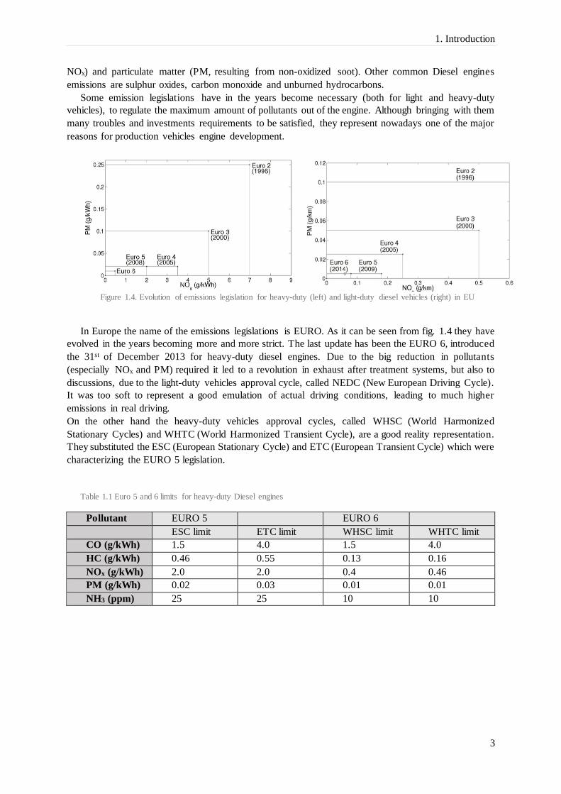
Some emission legislations have in the years become necessary (both for light and heavy-duty

vehicles), to regulate the maximum amount of pollutants out of the engine. Although bringing with them

many troubles and investments requirements to be satisfied, they represent nowadays one of the major

reasons for production vehicles engine development.

Figure 1.4. Evolution of emissions legislation for heavy-duty (left) and light-duty diesel vehicles (right) in EU

In Europe the name of the emissions legislations is EURO. As it can be seen from fig. 1.4 they have

evolved in the years becoming more and more strict. The last update has been the EURO 6, introduced

the 31st of December 2013 for heavy-duty diesel engines. Due to the big reduction in pollutants

(especially NOx and PM) required it led to a revolution in exhaust after treatment systems, but also to

discussions, due to the light-duty vehicles approval cycle, called NEDC (New European Driving Cycle).

It was too soft to represent a good emulation of actual driving conditions, leading to much higher

emissions in real driving.

On the other hand the heavy-duty vehicles approval cycles, called WHSC (World Harmonized

Stationary Cycles) and WHTC (World Harmonized Transient Cycle), are a good reality representation.

They substituted the ESC (European Stationary Cycle) and ETC (European Transient Cycle) which were

characterizing the EURO 5 legislation.

Table 1.1 Euro 5 and 6 limits for heavy-duty Diesel engines

Pollutant EURO 5 EURO 6

ESC limit ETC limit WHSC limit WHTC limit

CO (g/kWh) 1.5 4.0 1.5 4.0

HC (g/kWh) 0.46 0.55 0.13 0.16

NOx (g/kWh) 2.0 2.0 0.4 0.46

PM (g/kWh) 0.02 0.03 0.01 0.01

NH3 (ppm) 25 25 10 10

1. Introduction

4

1.2. Pollutants

1.2.1. NOx

NOx is a common term that stands for NO and NO2 compounds. NO2 is a brown toxic gas which can

cause serious damages both to vegetation and human respiratory tracts, resulting in one of the most

dangerous engine emissions.

Although the engine produces also NO, it will easily oxidize to NO2, contributing to acidification,

eutrophication and smog.

NOx production mechanisms can be divided in three categories :

Thermal NOx, created by the reaction of N2 with O2 present in air, at high temperatures. Its

production is described by the Zeldovich mechanism.

Prompt NOx, formed from reactions with HCN in fuel rich zones.

Fuel NOx, when the fuel releases the N bound as radical during the combustion.

However the first mechanism is by far the predominant one in combustion engines and thus in general

the higher the temperature reached during the combustion, the higher the NOx formation.

NOx is produced especially by diesel engines. Even though they have less out-of-cylinder NOx, due

to their lean mixture conditions, the catalyst has a lower effectivity and can’t reduce properly the out-

of-tailpipe NOx emissions, as it does in gasoline Otto engines.

Having around stoichiometric conditions, gasoline Otto engines reach higher temperature in the

combustion, leading to a higher NOx production. At the same time anyway the three way catalyst is at

its best NOx reduction rate, giving low emissions in the end.

1.2.2. PM

Particulate matter (PM), formed from soot, represents another health threat. It can create respiratory

problems, as well as cancer and cardiovascular diseases.

PM consists of porous carbon cores that absorb many different products as unburnt hydrocarbons from

oil and fuel, sulfuric acid, nitrogen acid, metals, ash and water.

Figure 1.5. Typical composition of particulate matter emitted from heavy-duty diesel engine operating under the test

cycle

One problem (or advantage) about PM is that it usually has a behaviour inversely proportional to

NOx emissions. Because when we do have high temperatures, and thus high NOx levels, soot is easily

oxidized. On the other hand with lower temperatures, and lower NOx formation, soot production is

increasing.

However it is usually common to keep the temperatures and NOx levels pretty high, and then try to

1. Introduction

5

reduce them, because it’s where the engine efficiency is the highest and therefore the fuel consumption

the lowest. This is the reason why the pursuit of good NOx reduction systems is so important.

The component responsible for the PM emissions reduction is the Diesel Particulate Filter (DPF),

which traps the particles passing through it. They could be closed filters, with better filtration

performances but requiring active regeneration and thus a fuel penalty, or open filters with passive

regeneration.

1.2.3. HC

Less problematic for diesel engines than for Otto engines, hydrocarbons, and especially PAHs (poly-

aromatic hydrocarbons), are carcinogenic and contribute to photochemical smog and ozone.

HC emissions are due to unburned hydrocarbons that can occur in different ways :

Overly lean or rich regions

Quenching against the cylinder liner

Occasionally from large fuel drops

Fuel ending in crevices between the piston and the cylinder liner

Desorption from the oil film on the cylinder liner

Misfire

However usually of these unburned HC a big fraction is partially combusted.

They can become important in two stroke engines, four stroke engines with long valve overlaps and

during cold start for SI-engines (spark ignited).

1.2.4. CO

Carbon monoxide is the last between the principal pollutants dangerous to humans. It is odourless,

colourless and highly toxic. Preventing the blood form carrying oxygen, at major exposure it can bring

to loss of consciousness and death.

It is usually a major product of rich combustion, but could also be formed by CO2 dissociation or by

quenching on cold surfaces. This is the worst emission in Otto engines with premixed combustion and

nearly absent in Diesel engines.

1.3. Diesel Oxidation Catalyst

The DOC is one of the principal exhaust after treatment components in Diesel engines. It has a pretty

similar structure to the 3-way catalyst used in Otto engines, but it is optimized on HC and NO oxidation.

As stated earlier this catalyst, due to the lean conditions in which the Diesel engine is running, is not

able to properly reduce NOx (fig. 1.6). Its functions are then :

Oxidation of CO : 2CO + O2 → 2CO2

Oxidation of HC : 4HC + 5O2 → 4CO2 + 2H2O

Oxidation of NO : 2NO + O2 → 2NO2

The latter oxidation is needed to increase the following SCR (Selective Catalytic Reduction)

performances.

1. Introduction

6

Figure 1.6. Three-way catalyst conversion efficiency

The DOC can be also used to oxidize post-injected fuel to increase temperature and help preheating

downstream components as well as actively regenerate the DPF, by oxidizing soot.

1.4. Methods of reducing NOx

One of the most important factors for a successful Diesel engine is a good fuel consumption, and this

happens when high efficiency conditions are reached. As formerly anticipated high efficiencies are

obtained with high combustion temperatures and therefore are simultaneous to high NOx production.

It is straightforward then to see how important it is to find a good way to reduce the NOx formed in the

combustion, because it allows directly to run at higher temperatures and improve fuel consumption.

The most common techniques developed in the last years to decrease NOx emissions are :

EGR

LNT

In cylinder control

SCR

1.4.1. EGR

EGR which stands for Exhaust Gas Recirculation, has been one of the most common ways to reduce

NOx emissions.

It consists in directing a portion of engine-out exhaust gases back to the intake manifold. The amount of

recirculated gas is controlled by the EGR valve.

1. Introduction

7

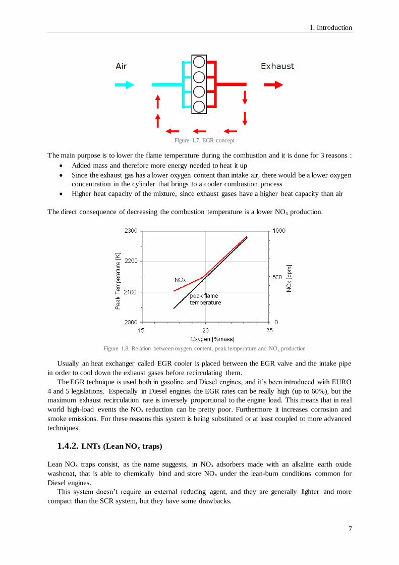
Figure 1.7. EGR concept

The main purpose is to lower the flame temperature during the combustion and it is done for 3 reasons :

Added mass and therefore more energy needed to heat it up

Since the exhaust gas has a lower oxygen content than intake air, there would be a lower oxygen

concentration in the cylinder that brings to a cooler combustion process

Higher heat capacity of the mixture, since exhaust gases have a higher heat capacity than air

The direct consequence of decreasing the combustion temperature is a lower NOx production.

Figure 1.8. Relation between oxygen content, peak temperature and NOx production

Usually an heat exchanger called EGR cooler is placed between the EGR valve and the intake pipe

in order to cool down the exhaust gases before recirculating them.

The EGR technique is used both in gasoline and Diesel engines, and it’s been introduced with EURO

4 and 5 legislations. Especially in Diesel engines the EGR rates can be really high (up to 60%), but the

maximum exhaust recirculation rate is inversely proportional to the engine load. This means that in real

world high-load events the NOx reduction can be pretty poor. Furthermore it increases corrosion and

smoke emissions. For these reasons this system is being substituted or at least coupled to more advanced

techniques.

1.4.2. LNTs (Lean NOx traps)

Lean NOx traps consist, as the name suggests, in NOx adsorbers made with an alkaline earth oxide

washcoat, that is able to chemically bind and store NOx under the lean-burn conditions common for

Diesel engines.

This system doesn’t require an external reducing agent, and they are generally lighter and more

compact than the SCR system, but they have some drawbacks.

1. Introduction

8

The biggest drawback is that the LNT system introduces fuel penalties. This is because the trap is

periodically saturating and therefore it needs to be regenerated, by running the engine under

stoichiometric or fuel-rich conditions for few seconds. In this way the NOx saturating the trap is desorbed

and then reduced to N2 and O2 in the downstream reduction catalyst (that can be a common 3-way

catalyst).

The storage capacity of the LNT is fixed, meaning that the higher the engine loads, the more frequently

it needs to be regenerated bringing to worse fuel consumption.

Moreover LNTs adsorb also sulphur oxides, requiring Diesel fuels with low sulphur content (below

15 ppm) and periodical desulphation cycles.

1.4.3. In cylinder control

This is the simplest way to reduce NOx emissions because it doesn’t require an additional system for the

exhaust aftertreatment.

It basically consists in adjusting the combustion process to keep low the NOx emission levels. These

strategies can be for example compression ratio reduction, use of two-stage turbocharging, variable

valve lift, combustion chamber reshaping or a reduction of fuel injection pressure.

In passenger cars, due to the type-approval test cycles (NEDC) that are not including high load

operations, these techniques can succeed in achieving even EURO 6 NOx levels without requiring further

components.

1.5. SCR

The selective catalytic reduction (SCR) is nowadays the most effective and common exhaust

aftertreatment technology used in heavy-duty Diesel engines to break down NOx emissions.

That is done through the use of a catalyst that thanks to the addition of a solution called AdBlue, is able

to reduce NOx to N2, sometimes with pretty high conversion efficiency.

The AdBlue is a solution of water and urea (32.5 %) which is injected in the hot exhaust gases at

temperatures above a certain threshold, since it needs to evaporate into CO2 and NH3, which is the real

reducing agent. Urea evaporation is usually a critical step and problems with deposit formation are pretty

common.

The chemical transformation that Urea ( (NH2)2CO ) should undergo in that process are :

(NH2)2CO →NH3+HNCO

HNCO+H2O →NH3+CO2

The higher the evaporation rate, and thus the NH3 concentration in the exhaust gases, the higher

would be the reduction performances in the downstream catalyst.

1. Introduction

9

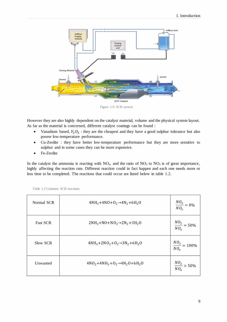
Figure 1.9. SCR system

However they are also highly dependent on the catalyst material, volume and the physical system layout.

As far as the material is concerned, different catalyst coatings can be found :

Vanadium based, 𝑉2𝑂5 : they are the cheapest and they have a good sulphur tolerance but also

poorer low-temperature performance.

Cu-Zeolite : they have better low-temperature performance but they are more sensitive to

sulphur and in some cases they can be more expensive.

Fe-Zeolite

In the catalyst the ammonia is reacting with NOx, and the ratio of NO2 to NOx is of great importance,

highly affecting the reaction rate. Different reaction could in fact happen and each one needs more or

less time to be completed. The reactions that could occur are listed below in table 1.2.

Table 1.2 Common SCR reactions

Normal SCR

4NH3+4NO+O2→4N2+6H2O

𝑁𝑂2

𝑁𝑂𝑥= 0%

Fast SCR

2NH3+NO+NO2→2N2+3H2O

𝑁𝑂2

𝑁𝑂𝑥= 50%

Slow SCR

4NH3+2NO2+O2→3N2+6H2O

𝑁𝑂2

𝑁𝑂𝑥= 100%

Unwanted

4NO2+4NH3+O2→4N2O+6H2O

𝑁𝑂2

𝑁𝑂𝑥> 50%

1. Introduction

10

The best ratio 𝑁𝑂2

𝑁𝑂𝑥 that can be achieved is then around 50%, because it allows a faster NOx reduction;

while the last reaction is marked as unwanted due to the N2O production, which is less dangerous but

still a pollutant.

As it can be seen from fig 1.10 the SCR is usually positioned downstream the DOC and the DPF.

This is a strategical choice, because the oxidation of NO to NO2 in the DOC can be used to adjust the 𝑁𝑂2

𝑁𝑂𝑥 ratio available at the SCR inlet. Furthermore it prevents much PM to enter the AdBlue evaporation

area and the SCR, avoiding many possible issues.

Figure 1.10. Example of a complete aftertreatment system

When too high temperatures are reached in the catalyst, it is likely to lose selectivity, bringing to

reactions that should absolutely be avoided, converting ammonia (NH3) in pollutants. They are:

4NH3+4O2→2N2O+6H2O

4NH3+5O2→4NO+6H2O

Finally an SCR system needs to be equipped with a so called Ammonia Slip Catalyst (ASC), that

prevents high levels of ammonia emissions, allowing at the same time an ammonia overflow which

increases the reactions speed. This catalyst should be highly selective and the desired reaction is

4NH3+3O2→2N2+6H2O

1.6. AdBlue chemistry

AdBlue is the commercial trademark used for the aqueous urea solution AUS32 (with 32,5 % of

technical urea) used in all SCR systems nowadays. The trademark is owned by the German association

Verband der Automobilindustrie (VDA).

Needless to say, it has to comply with strict requirements conformed with ISO 22241, in order to not be

detrimental to catalysts.

It can be produced basically in two ways: synthesis and dissolution.

In the first process, the most pure one, AdBlue is directly derived from ammonia/urea production process

and has no risks of contamination.

In the second one, dissolution, Urea is usually solidified and some substances are added to store and

preserve it. It’s from these additives that AdBlue can be contaminated with dangerous impurities.

1. Introduction

11

A key aspect to be considered is also AdBlue conservation. Correct temperatures, that can ensure a

duration of 12 months after its production, vary between -10 and 30 ℃. Usually the freezing (below -11

C) has no impact on AdBlue quality, while temperatures higher than 30 ℃ reduce its life rather sharply.

1.6.1. Urea

The urea is a compound of carbon, nitrogen, hydrogen and oxygen, with chemical composition

CO(NH2)2 that could be find solid in nature, being crystalline at room temperature. Its structure can be

seen in fig 1.11 and the group NH2 is called amino group.

Figure 1.11. Urea chemical structure

At high temperatures it undergoes phase transitions. Its melting point is at 406.5 K, with a fusion

enthalpy of 14.79 kJ/mol, as it was determined by Gatta and Ferro [1]. It is colourless and odourless,

has a high solubility in water, and is not toxic.

Urea, due also to its extensive usage in different fields, as agriculture (used as fertilizer, one of urea

most common uses), chemical industry, explosives, automobile systems, medical applications, and

others, is produced worldwide on a big scale. It’s noteworthy that in 2012 the worldwide production

capacity was around 184 million tonnes.

The production (with a process called Bosch-Meiser) consists of the synthesis starting from ammonia,

NH3, and carbon dioxide, CO2, with two consecutive reactions, with ammonium carbamate as an

intermediate product.

2NH3+CO2 ⇄ H2N-COONH4

H2N-COONH4 ⇄ (NH2)2CO+H2O

The first reaction can occur only at high pressures, therefore in the exhaust systems there won’t be any

issue related to the damages due to ammonium carbamate, which is a highly corrosive species.

In any case, in order to be useful for its purpose, i.e. NOx reduction in the SCR catalyst, urea should

undergo its decomposition in favour of reducing agents, ammonia and isocyanic acid.

The urea decomposition starts at high temperatures and follows

(NH2 )2CO → NH3+HNCO

In addition isocyanic acid can further be hydrolysed to generate ammonia and CO2, although this occurs

only at a temperature above 400 °C.

HNCO+H2O → NH3+CO2

A decomposition trend could be seen in fig. 1.12, where it is represented the nitrogen distribution

between the three species (ammonia, isocyanic acid and urea), at the catalyst entrance, as a function of

temperature.

1. Introduction

12

Figure 1.12. Urea decomposition trend

Urea evaporation takes place both in the gaseous phase and on the walls. This second case is the most

critic one, since when urea decomposes it is possible to get into by-products formation, which can foul

the SCR catalyst, as well as form deposits in the evaporation unit.

Several are the by-products that could be formed, and in the following lines a brief list of them, with

their characteristic reactions, is presented.

Biuret (favourable from 160 °C up to 200 °C) [2, 3, 4]

NH2CONH2 + HNCO ⇄ NH2CONHCONH2

Cyanuric acid (favourable above 190, up to 340 °C) [4]

NH2CONHCONH2 + HNCO → cyanuric acid + NH3

2NH2CONHCONH2 → cyanuric acid + HNCO + 2NH3

NH2CONHCONH2 + NH2CONH2 → cyanuric acid + 2NH3

3HNCO → cyanuric acid

However above 350 °C no new solid deposits are formed, and the decomposition of cyanuric acid back

to isocyanic acid starts.

cyanuric acid →3HNCO

Ammelide [2, 4]

cyanuric acid + NH3 → ammelide + H2O (above 300 °C)

NH2CONHCONH2 + HNCO → ammelide + H2O (lower than 300 °C)

2NH2CONHCONH2 → ammelide + HNCO + NH3 + H2O (lower than 300 °C)

Ammeline (favourable above 250 °C) [2, 4]

ammelide + NH3 → ammeline + H2O

1. Introduction

13

Melamine (favourable above 250 °C) [4]

ammeline + NH3 → melamine+ H2O

Figure 1.13. Urea by-products morphology

1.6.2. NH3

NH3, known also as ammonia, is a colourless gas, lighter than air and with a pungent smell. This

compound of nitrogen and hydrogen could be found in nature in the gaseous form, due to its low boiling

temperature at the pressure of one atmosphere. Nevertheless, it has a high solubility in water and this

can cause wet deposition, when it dissolves in atmospheric water vapour.

It is rather reactive, corrosive and toxic. If inhaled this substance can create irritation and pain to the

respiratory system, and in the worst cases can be fatal.

The boiling and melting points, being respectively -33,5 °C and -77,7 °C, are significantly higher

than the ones characteristic of compounds of the same kind, and this means a higher liquefiability, thanks

to the strong hydrogen bonding existing between the molecules.

The geometry of the molecule is a non-planar triangular pyramid that we can visualize in fig. 1.14.

Figure 1.14. Ammonia chemical structure

The four electrons pair repels each other giving to the molecule the shape seen above, and this is cause

of a high polarity that promotes the hydrogen bonding and explains to some extent its high solubility in

water.

Furthermore the dissolution in water leads to a chemical reaction, where ammonia acts as a base and,

subtracting hydrogen ions from H2O, becomes ammoniun and generates hydroxide ions. This

production of ions is what gives to aqueous solutions of ammonia the important alkaline properties.

NH3+H2O ⇄ NH4++OH-

1. Introduction

14

1.7. Problem description

So far the SCR is the most effective procedure to break down this kind of emissions, but it would be

even more effective if we could achieve a perfect balance of reactants and temperatures, and a good

evaporation of the ammonia from Urea.

Another issue with the last mentioned process is to avoid build-up of Urea deposits in the evaporation

unit, cause it will limit the SCR performances, increase the probable repairs needed, and last but not

least create a backpressure on the engine that increases fuel consumption. A technique to take away urea

deposits is to run few hotter cycles, but it penalizes fuel consumption. Therefore, it is of vital importance

for the automotive manufacturers to extract the most out of this system, in order to be competitive on

the market and to comply with the new regulations.

The evaporation module for the so called large silencer (used for Scania trucks with V8 engines),

which is the one that will be analysed, consists of two concentric pipes, a deflector and a dosing unit,

positioned downstream the DOC (Diesel Oxidation Catalyst) and the DPF (Diesel Particulate Filter)

and upstream the SCR and ASC (Ammonia Slip Catalyst).

Figure 1.15. Silencer assembly 3D section with component detail

The exhaust gases are directed to this unit, and naturally split between the inner tube and the outer

annulus, while the deflector gives a rotational movement to the gases. This is done to push the urea

droplets against the walls of the inner tube, increasing the area hit by them and hence increasing urea

evaporation rate. In order to achieve a good rate, is straightforward to see that a high temperature has to

be reached on the inner pipe walls, and this is helped by a finned outer surface (of the inner pipe) which

increases the heat transfer between exhaust gases and the pipe wall. In many cases, anyway, it’s been

observed some deposit build-up, causing not only a drop in performances but also a backpressure

increase. Studies and tests have been carried-on about deposit formation, and the results are going to be

summarized in the next paragraph.

Moreover, the production of the finned inner pipe is pretty expensive, since those flanges are created

by first folding a thin sheet of metal and then by laser welding them (with a unique robot) on the tube

already manufactured. This, as can be imagined, involves costly tooling and process (there are

approximately 52 m of welding in a single component).

1. Introduction

15

Figure 1.16. Fins detail

The purpose of the work then is to study a new design of the evaporation inner pipe, to achieve a

lower production cost, maintaining or even increasing the evaporation performances (i.e. to get a lower

deposit formation and a better evaporation).

1.7.1. Urea deposit formation

The common deposits that can occur on surfaces in contact with urea environment are of two kinds :

Deposits of urea (from the AdBlue solution), that are crystalline and melt easily at typical

exhaust gas temperatures

Deposits of byproducts, resulting from the chemical reactions seen in 1.6.1, that form a sticky

substance and are critical to be removed.

Figure 1.17. Deposits behaviour with a variable temperature

In the desired urea evaporation reaction, in addition to urea, isocyanic acid is being produced as a partial

result. It should be then hydrolysed into other ammonia and carbon dioxide but being a stable gas at

high temperatures and having high tendency to react with other molecules, it plays a key role in solid

deposits formation.

As showed in chapter 1.6.1, the main by-products types, depending on the temperature, are cyanuric

acid, ammelide, ammeline, melamine and biuret. Their quantity dependence on the temperature reached

are displayed in fig. 1.17. Its formation begin earliest at 150 ℃.

0

20

40

60

80

100

100 150 200 250 300 350 400 450Temperature [°C]

Ma

ss [%

]

total rcovery

urea

biuret

ammelide

cyanuric acid

1. Introduction

16

The solid deposits forming at high temperatures are also the more difficult deposits to remove and this

is the reason why they should be totally avoided.

The reactions that bring to the solid products build up are favourable within big accumulations of

urea and big film heights. To prevent big liquid urea stacks obstacles and edges must be avoided, leaving

urea able to flow into uncritical areas, and urea evaporation must be enhanced. The urea evaporating

rate is proportional to the film surface, therefore a bigger wet area helps the evaporation not only by

decreasing the temperature drop on the pipe, but also giving a bigger surface available for the urea

evaporation.

It is straightforward to see that a bigger AdBlue mass flow will lead to bigger temperature drops and a

bigger film formation. Therefore for each combination of exhaust gases mass flow and temperature a

limit in the AdBlue dosing must be respected.

However the higher the temperatures reached in the pipe, the lower the film formation, with a

constant amount of AdBlue dosing, and therefore the lower the risk of deposits. Furthermore, from fig

1.18 it can be seen that above certain temperatures (around 400 ℃) also the toughest solid deposits are

going to be removed.

That is one of the main reasons why heat flanges have been introduced to enhance the heat transfer

from the exhaust gases to the pipe and hence heat up the pipe, reducing the solid products deposit.

The optimization of the pipe’s design is thus to keep the pipe to the highest possible temperature, in

order to shift at higher dosing quantities the same amount of molten urea film on the walls and therefore

the deposits build-up.

Figure 1.18. Deposit formation on a hot plate

At the same time, allowing a higher dosing, and a better evaporation, will bring to an increased amount

of ammonia available in the SCR downstream, and eventually an improved NOx reduction.

1.7.2. Methodology

To sum up the purpose of the thesis is to study the evaporation unit and find a new design that can :

Reduce manufacturing costs

Increase or at least keep the current evaporation performances

1. Introduction

17

In order to achieve the stated objectives 5 steps will be necessary :

Heat transfer analysis trough correlations, as a first evaluation of the influence of the fins

geometry and number. Using those results an FEM analysis is then carried on to understand the

thickness and conductivity weight.

Study of possible materials alternatives

Investigation of manufacturing process alternatives

CFD simulations to get detailed information of the important parameters that could introduce

improvements in performances

Actual testing of dosing plates, to verify the previous results

Some project constraints are necessary and they will be :

The dosing unit and its position, being a consolidated component

The outer pipe, being restricted in dimension by the other silencer organs

The mixer design and its position, having been already examined in depth

The inner surface, which should be as smooth as possible to prevent urea deposits and not too complex

to avoid a cost increment.

1.8. Scania silencers family

Scania CV AB produces for its trucks three different engines families with different power output ranges,

which are the 5 cylinders inline, 6 cylinders inline and V8 engines and go from 250 hp to 730 hp. The

V8 group has a power output between 520 and 730 hp. Furthermore being Scania active on markets all

over the world, different regulations compliance are needed, basically ranging from Euro 4 to Euro 6.

This is why three different after-treatment systems, with different encumbrances, have been developed.

They are respectively the Large silencer, the Medium silencer and the Common silencer. They take their

names from their dimensions.

The Large silencer is the bigger one with a length of 900 mm and the configuration showed in fig.

1.15. It is employed in all Euro 6 V8 engines, and the evaporation unit is the one that will be studied in

this thesis work.

The Medium silencer is characterized by a smaller dimension, with a length of 623 mm and a

different evaporation pipe configuration. It is used in all 5 and 6 cylinders engines following the Euro 6

regulations. In fig. 1.19 it can be seen how it differs from the large silencer. The flow is directed on a

finned end plate, which deflects it and makes it move backwards. After a short path it is turned again

forwards, continuing in the SCR. In this way the flow touches more than one time each pipe’s wall,

heating them up, in order to increase the urea evaporation rate.

In the end the common silencer is the smallest one and is used in engines following Euro 5 regulations

and lower. It doesn’t have any evaporation pipe, but the AdBlue is sprayed in a common volume after

the exhaust gases inlet. Also the DOC and the DPF are missing in this version, and it is straightforward

to see the lower aftertreatment performances.

1. Introduction

18

Figure 1.19. Medium silencer section

19

2. Heat Transfer Analysis

This chapter is intended to study the heat transfer occurring through the walls of the evaporation pipe,

and thus how the heat is transferred to the evaporating urea. After a brief introduction on the heat transfer

theory, a first evaluation of the different geometries will be made by analysing the overall heat transfer

coefficient of each solution, varying number of fins (and width) and their height. Correlations will be

used to compute the convective coefficients. In the end those coefficients will be used in FEM models,

to compute the temperature drops obtained with certain urea distributions, and evaluate the thickness

and material conductivity influence.

2.1. Heat transfer theory

Heat could be defined as the energy form which spreads through system borders due to a temperature

difference.

At the basis of heat transfer theory, in addition to the two principles of thermodynamics and mass and

momentum conservation equations, relations relative to the three different phenomena participating in

the heat transfer need to be taken into account. They are Fourier’s law for conduction, Newton’s law for

convection and Stefan-Boltzmann’s law for irradiation.

Although in most real situations those 3 processes co-exist, they can be studied separately and then

superimposed the resulting effects.

This is basically the reason, in addition to the pursuit of simplicity, why in the following work irradiation

between the inner and the outer pipe, and in the fins calculations will be neglected. If we consider that

in a given operating point the temperature of the outer pipe would be roughly constant for every different

design, the irradiation would have almost the same impact on the inner pipe. It would potentially help

the worse solutions by raising their lower temperature, but in this case it is considered to be neglectable.

2.1.1. Conduction

Thermal conduction is the transfer of heat due to a temperature difference that happens to substances,

in all phases (gases, liquids, solids and plasmas). It is governed by microscopic vibration and collisions

between elementary objects as molecules, atoms, phonons and electrons, and motion, diffusion of

electrons, that transfer internal energy (i.e. the sum of kinetic and potential energy).

The heat transferred is function of both temperature difference and a variable that represents the

material ability to transfer heat, thermal conductivity.

Thermal conductivity is defined as “the quantity of heat (∆𝑄) transmitted in time (∆𝑡) through a

thickness ∆𝑥, in a direction normal to a surface of area 𝐴, due to a temperature difference ∆𝑇” and is

expressed with the letter 𝒌. It can thus be written

𝑘 = −

∆𝑄

∆𝑡

1

𝐴

∆𝑥

∆𝑇

(2.1)

[𝑘] =

𝑊

𝑚 𝐾

(2.2)

which comes from the integral form of the heat conduction law.

2. Heat Transfer Analysis

20

∆𝑄

∆𝑡= −𝑘𝐴

∆𝑇

∆𝑥

(2.3)

The differential form at the base of heat conduction (called Fourier’s law) can be obtained, but here for

simplicity it is just going to be showed how it looks like :

�⃗� = −𝑘∇𝑇 (2.4)

where �⃗� is the local heat flux density (𝑊

𝑚2), 𝑘 is the thermal conductivity and ∇𝑇 is the temperature

gradient (𝐾

𝑚). If 𝑘 is considered constant it is easy to see how the Fourier’s law can be integrated leading

to the integral form. The minus sign means that when the temperature is decreasing with 𝑥, the thermal

flux flowing in the x direction is positive.

Thermal conductivity is highly dependent on medium’s phase, temperature, density and molecular

bonding. In fact, in solids and especially metals heat conduction is by far the predominant phenomenon.

This is due to their structure which facilitates energy transferring through vibrations and to the metallic

bonds that allow electrons to move and thus transfer thermal energy quickly.

On the other hand fluids, having larger inter-atomic distances, they are subject to fewer collisions

and thus lower conduction.

In insulators instead, the biggest contribution in heat transfer is brought by phonon vibrations.

2.1.2. Convection

Thermal convection is a heat transfer combined process, introduced by fluids movements that modify

the nature of the heat transfer phenomenon. It is therefore absent within solid bodies.

The quantitative relation describing the global effect of convection between solids and fluids is

known as Newton’s law and can be written as

�⃗� = ℎ (𝑇𝑤 − 𝑇𝑓) �⃗⃗� (2.5)

[ℎ] =𝑊

𝑚2 𝐾

(2.6)

Where �⃗� is the heat flux per unit area, 𝑇𝑤 is the wall temperature, 𝑇𝑓 is the fluid temperature and ℎ is

the convection coefficient.

This latter coefficient is usually result of complex relations and function of geometries, physical

properties and thermodynamics conditions of the process.

Assuming that the speed at the interface between the fluid and the solid is null due to the adhesion

condition, it seems that the temperature gradient at the wall, and thus the heat flux transferred, can be

evaluated just by considering pure conduction.

But, the temperature gradient at the wall is also dependent on the quickness with whom the fluid is

taking away heat, which is directly related to the fluid’s speed.

In convection analysis it is therefore really important to know the speed field, since it has massive

influence on the thermal field.

Depending on fluid motion causes, convection can be divided into natural convection, when the

motion is due to temperature gradients, and forced convection, when the motion is induced by an external

action.

2.1.3. Irradiation

This process is different from the others because it doesn’t require material support, happening by means

of electromagnetic waves the irradiation heat transfer.

2. Heat Transfer Analysis

21

Two bodies are subject to heat exchange by simultaneously emitting and absorbing electromagnetic

radiation which is (partially) converted into internal energy. The emitted energy is directly proportional

to the temperature of the body and the net amount of transferred heat is the difference between the two

fluxes. The general relation for grey bodies is:

𝑞 = 𝐹𝜖 𝐹𝑔 𝜎 (𝑇14 − 𝑇2

4) (2.7)

where 𝜎 is the Stefan-Boltzmann constant (5,669 ∙ 10−8 𝑊

𝑚2 𝐾4) , 𝐹𝜖 is the emissivity factor and 𝐹𝑔 is

the view factor.

The emissivity factor depends on the surface properties as material, etc. and is usually lower than 1

(equal to one just for a black body), while the view factor depends on the geometry of the problem and

the relative positioning of the bodies and is also equal to one just for black bodies. It is therefore

straightforward to obtain the Stefan/Boltzmann law for black bodies.

𝑞 = 𝜎 (𝑇14 − 𝑇2

4) (2.8)

2.1.4. Conduction equation

In most cases, and that’s what it is later on an FEM software going to be used for, the aim of heat

conduction study is to compute the temperature distribution within the bodies. In order words to get the

function

𝑇 = 𝑓(𝑥, 𝑦, 𝑧, 𝑡) (2.9)

To do so, a good tool that can be used is the general conduction equation, i.e. nothing else than an energy

balance of a volume subject to heat transfer through conduction.

With some simple hypothesis [6], from the balance of an infinitesimal element it can be obtained

∇(𝑘 ∇𝑇) + �̇� = 𝜌 𝑐

𝜕𝑇

𝜕𝑡

(2.10)

That can be rewritten as

𝑎 ∇2𝑇+

�̇�

𝜌 𝑐= 𝜕𝑇

𝜕𝑡

(2.11)

Where 𝑎 is thermal diffusivity (𝑚2

𝑠), �̇� internal heat generation and 𝑐 material’s specific heat.

And in case of steady-state, without internal heat generation, we have

∇2𝑇 = 0 (2.12)

which is called Laplace differential equation.

Boundary Conditions

In order to be solved the equation and then to study a conduction process, some mathematical conditions

representing the process need to be added as “constraints”, as well as initial conditions in the case of a

transient regime.

2. Heat Transfer Analysis

22

These conditions should to be applied to the geometrical boundary of the domain and they’re

therefore called boundary conditions. Four different kinds of boundary conditions should be considered :

1. Dirichlet condition :

It consists in specifying the temperature on the surface of the body. If the temperature is uniform

and constant during the process it means setting

𝑇𝑠 = 𝑐𝑜𝑠𝑡 (2.13)

2. Neumann condition :

It consist in specifying the derivative of the temperature in a perpendicular direction to the

surface. It is equivalent to setting in each point the heat flux density

𝑞 = −𝑘 (

𝜕𝑇

𝜕𝑛)𝑠= 𝑓(𝑥, 𝑦, 𝑧, 𝑡)

(2.14)

3. Robin condition :

It consists in applying a proportional relation between the derivative of the temperature

perpendicularly to the surface and the surface temperature itself. This condition is typical when

convection at the boundary surface is involved, and therefore we can write

𝑞 = −𝑘 (

𝜕𝑇

𝜕𝑛)𝑠= ℎ (𝑇𝑠 − 𝑇∞)

(2.15)

4. 4th type condition :

This is common in interfaces between bodies with different thermal conductivity and consists

in equalizing the flux through the contact surface.

𝑘1 (

𝜕𝑇1

𝜕𝑛)𝑠= 𝑘2 (

𝜕𝑇2

𝜕𝑛)𝑠

(2.16)

The listed boundary conditions, and especially the second and third one, will be used in the FEM analysis

later on, to emulate the convection of the gases all over the pipe, and the heat flux absorbed by the urea

presence on the inner surface.

It is finally of interest, having a cylindrical problem, to get the results of the conduction equation for

a steady-state cylindrical problem. This solution is going to be used to evaluate the heat transferred in

the evaporation pipe case.

Assuming to have uniform temperatures at the inner and outer surface of the pipe, the problem can be

simplified in a 1-D case, where the temperature is only function of the radius.

𝑇 = 𝑓(𝑟) (2.17)

We can therefore write from the Laplace differential equation

{

𝑑2𝑇

𝑑𝑟2+1

𝑟

𝑑𝑇

𝑑𝑟= 0

𝑇(𝑟𝑜𝑢𝑡 ) = 𝑇𝑜𝑢𝑡

𝑇(𝑟𝑖𝑛) = 𝑇𝑖𝑛

(2.18)

2. Heat Transfer Analysis

23

Which can be solved obtaining

𝑇(𝑟) = 𝑇𝑖𝑛 +

𝑇𝑖𝑛 −𝑇𝑜𝑢𝑡

ln𝑟𝑖𝑛𝑟𝑜𝑢𝑡

ln𝑟

𝑟𝑖𝑛

(2.19)

and

𝑞 =

𝑇𝑖𝑛 −𝑇𝑜𝑢𝑡1

2𝜋 𝐿 𝑘ln𝑟𝑜𝑢𝑡𝑟𝑖𝑛

(2.20)

Figure 2.1. Similar configuration of the evaporation module

2.2. Heat transfer calculations

2.2.1. Convection correlations

As already mentioned, great part of the convection study is to accurately evaluate the convection

coefficient, ℎ. Each different condition has its own relations and equations, and therefore it is important

to understand where the study case is located.

Being a pipe in pipe configuration, with the longitudinal flow flowing both in the inner region and the

outer annulus region, and being the exhaust gases “pushed” through the evaporator module, this is the

case of forced internal convection.

In order to find the correlation between the convection coefficient and the quantities influencing the

phenomenon, the Buckingham Theorem and dimensional analysis is going to be used.

The independent variables affecting the forced convection in a cylindrical duct are the geometrical

dimensions of the pipe (hydraulic diameter 𝑑), the fluid dynamic conditions in the duct (average velocity

𝑣), and the thermo-physical properties of the fluid (density 𝜌, dynamic viscosity 𝜇, thermal conductivity

𝑘 and specific heat 𝑐𝑝).

The correlation can thus be written as

ℎ = 𝑓(𝑑, 𝑣,𝜌, 𝜇, 𝑘, 𝑐𝑝) (2.21)

Applying then the Buckingham Theorem, and thus trying to get a series of a-dimensional parameters

describing the phenomenon, three a-dimensional quantities can be obtained:

2. Heat Transfer Analysis

24

- Reynolds Number, which represents the ratio between inertial and viscous forces acting on the

fluid

𝑅𝑒 =

𝑣 𝑑 𝜌

𝜇

(2.22)

- Nusselt Number, which represents the ratio between heat convection and conduction in the fluid

𝑁𝑢 =

ℎ 𝑑

𝑘

(2.23)

- Prandtl Number, which represents the ratio between momentum diffusion transport and heat

diffusion transport

𝑃𝑟 =𝜇 𝑐𝑝

𝑘 (2.24)

The phenomenon can thus be described by an easier relation between just these a-dimensional numbers

of the kind

𝑁𝑢 = 𝑓(𝑅𝑒, 𝑃𝑟) (2.25)

It needs to be stressed out also the importance of the hydraulic diameter which can be calculated as

𝑑 =

4 𝐴

𝑝

(2.26)

and has a great influence in the evaluation of ℎ.

The first a-dimensional number considered, the Reynolds number, plays a big role because it is the

discriminating factor between different motion regimes, and thus different relations describing the

convection.

For low Reynolds numbers (𝑅𝑒 ≤ 2300) the flow is said to be laminar; the viscosity is the

“predominant” factor leading to lower heat transfer coefficients, and the stream lines are orderly.

For high Reynolds numbers (𝑅𝑒 > 10000), the flow is turbulent, with high irregularities and local

velocity fluctuations.

For Reynolds numbers between 2300 and 10000 the transition region can be found, and the

correlations regulating it are complex and uncertain.

The correlations that are going to be used in this work are summarized in the following section.

Laminar flow (Hausen correlation, 1943)

𝑁𝑢 = 3.66 +

0.668 𝑅𝑒 𝑃𝑟 (𝑑/𝐿)

1 + 0.40 [𝑅𝑒 𝑃𝑟 (𝑑/𝐿)]2/3

(2.27)

Which can be used for both liquids and gases with constant wall temperature.

Transition region (Hausen correlation, 1943)

𝑁𝑢 = 0.116 [(

𝜌 𝑣 𝑑

𝜇)2/3

− 125] 𝑃𝑟1/3 (𝜇

𝜇𝑠)0.14

[1 + (𝑑

𝐿)2/3

] (2.28)

Turbulent flow (Petukhov correlation, 1970)

2. Heat Transfer Analysis

25

𝑁𝑢 =

(𝑓/8) 𝑅𝑒 𝑃𝑟

1.07 + 12.7 (𝑓/8)1/2 (𝑃𝑟2/3 − 1)

(2.29)

Where 𝑓 is the friction factor and which is valid for 0.5 < 𝑃𝑟 < 2000 and 104 < 𝑅𝑒 < 5 ∙ 106.

2.2.2. Friction factor and Pressure losses

As it will be explained later on it is of interest to evaluate the pressure drops along the pipe due to

distributed losses caused by friction.

The expression that can be used to evaluate them for flow in a pipe is

∆𝑝

𝜌= 𝑓

𝐿

𝑑

𝑣2

2

(2.30)

Being then usually known every variable except from the friction factor 𝑓, the problem turns into the

correct evaluation of that quantity.

The common tool used for this purpose for pipe flows is the Moody chart, which represents the

friction factor as a function of Reynolds number and the relative roughness.

For our purpose however it is convenient to use friction factor formulas. There are many formulas

available and they differ also for every type of flow that could occur.

Within laminar flow conditions and thus with 𝑅𝑒 < 2300 the friction factor doesn’t depend on the

roughness of the surfaces but only on the Reynolds number itself, according to

𝑓 =

64

𝑅𝑒

(2.31)

For bigger Reynolds numbers instead, the most commonly used relationship is the Colebrook-Whi te

equation (valid for 𝑅𝑒 > 4000 in conducts completely full of fluid)

1

√𝑓= −2 log (

𝑒

3.7 𝑑+

2.51

𝑅𝑒 √𝑓)

(2.32)

Where 𝑒 is the roughness of the pipe’s surface. Some common values of roughness are listed in table

2.1.

Table 2.1 Average roughness values for commercial pipe materials [5]

Material 𝒆 (mm)

Concrete 0.30-3.00

Wood stave 0.18-0.90

Riveted steel 0.90-9.00

Cast iron 0.26

Galvanized iron 0.15

Asphalted cast iron 0.12

Commercial steel 0.046

Wrought iron 0.046

Drawn tubing 0.0015

Machined steel 0.0008-0.0032

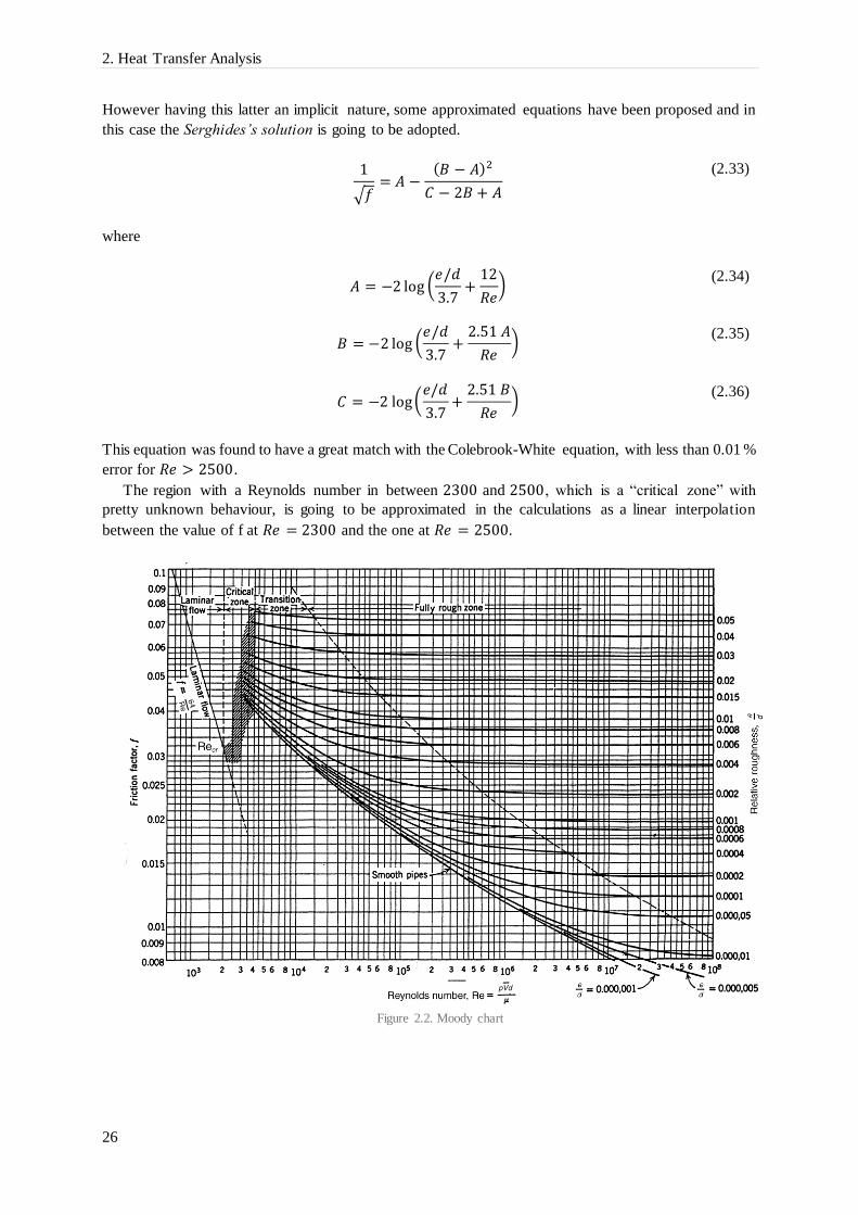
2. Heat Transfer Analysis

26

However having this latter an implicit nature, some approximated equations have been proposed and in

this case the Serghides’s solution is going to be adopted.

1

√𝑓= 𝐴 −

(𝐵 − 𝐴)2

𝐶 − 2𝐵 + 𝐴

(2.33)

where

𝐴 = −2 log (

𝑒/𝑑

3.7+12

𝑅𝑒)

(2.34)

𝐵 = −2 log (

𝑒/𝑑

3.7+2.51 𝐴

𝑅𝑒)

(2.35)

𝐶 = −2 log(

𝑒/𝑑

3.7+2.51 𝐵

𝑅𝑒)

(2.36)

This equation was found to have a great match with the Colebrook-White equation, with less than 0.01 %

error for 𝑅𝑒 > 2500.

The region with a Reynolds number in between 2300 and 2500, which is a “critical zone” with

pretty unknown behaviour, is going to be approximated in the calculations as a linear interpolation

between the value of f at 𝑅𝑒 = 2300 and the one at 𝑅𝑒 = 2500.

Figure 2.2. Moody chart

2. Heat Transfer Analysis

27

2.2.3. Hypotesis

In order to simplify the calculations and to get a first evaluation of the difference in the heat transfer

performances of different designs, some assumptions will be made.

First of all, it’s easy to understand that the sprayed AdBlue hitting the inner surface of the pipe, can

be represented on a heat transfer point of view as an heat sink which is absorbing heat. In this first phase

nevertheless, since it’s intended to compare the ability of transferring heat from the annulus to the inner

surface, two constant flow temperatures have been assumed, and the product 𝑈𝐴 is going to be analysed.

They can be seen as the average temperature over the pipe and they are both 200 °C for the annulus

region and for the inner region (the one where AdBlue is sprayed).

Furthermore being the complete silencer insulated and thus reaching inside it high temperatures, the

outer pipe’s wall will be considered adiabatic.

To make a good estimate on how the mass flow is going to be divided between the two regions, an

iteration will be done, to find the flow distribution that causes the same distributed (static) pressure drop

over the two paths. In this way, the higher the friction over a region, the lower the speed is going to be

in that region, in order to create the same pressure drop.

In the end, since the pressure drops are small the average pressure over the pipe is considered to be

close to the atmospheric pressure and thus the gas properties used are at 101330 𝑃𝑎.

The gas used in the calculations is air, since it’s been evaluated that by neglecting the combustion

products the error associated is usually less than 2% [7]. The air properties used are listed in appendix

A. In addition, being gases and already filtered by the DPF no fouling resistance will be considered.

Figure 2.3. Evaporation unit section

In fig. 2.3 a section of the evaporation module is shown, together with the most important dimensions.

In this first step 5 different fin geometries are going to be analysed. They are respectively rectangular

solid longitudinal fins (a), triangular solid longitudinal fins (b), the current design (c), radial rectangular

solid fins (d) and U shape fins (e), showed in fig. 2.4. They have been conceived by taking into account

the techniques that can be used to manufacture them. For that reason the shape, in order to not generate

a too expensive production cost, couldn’t be too complex.

However, first of all a simple pipe is going to be analysed.

2. Heat Transfer Analysis

28

Being for the AdBlue evaporation the lower temperatures with lower mass flows the most critical

conditions, the mass flow used in the following calculations it’s been assumed as 450 𝑘𝑔/ℎ. Normal

operation has a mass flow entering the evaporator between 450 and 2000 kg/h and temperature between

200 and 400 ℃.

a) b)

c) d)

Figure 2.4. Five different designs analysed in this first phase. a) SRL, b) STL, c) current design, d) SRR and e) U shape design

e)

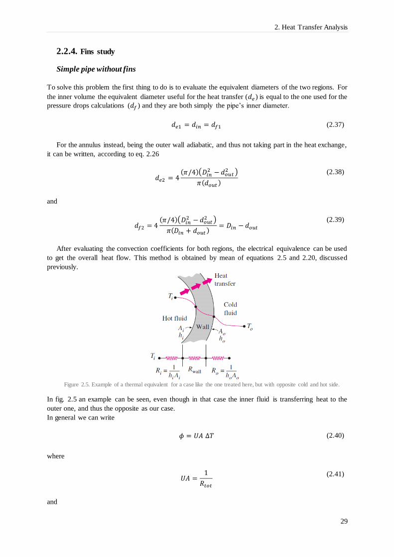
2. Heat Transfer Analysis

29

2.2.4. Fins study

Simple pipe without fins

To solve this problem the first thing to do is to evaluate the equivalent diameters of the two regions. For

the inner volume the equivalent diameter useful for the heat transfer (𝑑𝑒 ) is equal to the one used for the

pressure drops calculations (𝑑𝑓 ) and they are both simply the pipe’s inner diameter.

𝑑𝑒1 = 𝑑𝑖𝑛 = 𝑑𝑓1 (2.37)

For the annulus instead, being the outer wall adiabatic, and thus not taking part in the heat exchange,

it can be written, according to eq. 2.26

𝑑𝑒2 = 4

(𝜋/4)(𝐷𝑖𝑛2 −𝑑𝑜𝑢𝑡

2 )

𝜋(𝑑𝑜𝑢𝑡 )

(2.38)

and

𝑑𝑓2 = 4

(𝜋/4)(𝐷𝑖𝑛2 −𝑑𝑜𝑢𝑡

2 )

𝜋(𝐷𝑖𝑛 + 𝑑𝑜𝑢𝑡 )= 𝐷𝑖𝑛 − 𝑑𝑜𝑢𝑡

(2.39)

After evaluating the convection coefficients for both regions, the electrical equivalence can be used

to get the overall heat flow. This method is obtained by mean of equations 2.5 and 2.20, discussed

previously.

Figure 2.5. Example of a thermal equivalent for a case like the one treated here, but with opposite cold and hot side.

In fig. 2.5 an example can be seen, even though in that case the inner fluid is transferring heat to the

outer one, and thus the opposite as our case.

In general we can write

𝜙 = 𝑈𝐴 Δ𝑇 (2.40)

where

𝑈𝐴 =

1

𝑅𝑡𝑜𝑡

(2.41)

and

2. Heat Transfer Analysis

30

𝑅𝑡𝑜𝑡 = 𝑅𝑖𝑛 + 𝑅𝑤𝑎𝑙𝑙 + 𝑅𝑜𝑢𝑡 =

1

ℎ𝑖𝑛𝐴𝑖𝑛+ln(𝑑𝑜𝑢𝑡/𝑑𝑖𝑛)

2𝜋 𝑘 𝐿+

1

ℎ𝑜𝑢𝑡𝐴𝑜𝑢𝑡

(2.42)

It can therefore be written

𝑈𝐴 = 𝑈𝑖𝑛𝐴𝑖𝑛 = 𝑈𝑜𝑢𝑡𝐴𝑜𝑢𝑡 =

1

1ℎ𝑖𝑛𝐴𝑖𝑛

+ln(𝑑𝑜𝑢𝑡/𝑑𝑖𝑛)2𝜋 𝑘 𝐿

+1

ℎ𝑜𝑢𝑡𝐴𝑜𝑢𝑡

(2.43)

It can be observed that the overall heat transfer coefficient is dependent on the surface to which it is

referred to, assuming then different expressions and values.

The heat flux is then

𝜙 =

𝑇𝑖𝑛 − 𝑇𝑜𝑢𝑡1

ℎ𝑖𝑛𝐴𝑖𝑛+ln(𝑑𝑜𝑢𝑡/𝑑𝑖𝑛)2𝜋 𝑘 𝐿

+1

ℎ𝑜𝑢𝑡𝐴𝑜𝑢𝑡

(2.44)

Finned external surface

Fins are commonly added to surfaces to enhance heat transfer. In this case they have been added to the

external surface just to avoid possible urea deposits on the inner surface, where urea is sprayed. For this

reason the inner surface is considered as a constraint, having to be as smooth as possible.

Heat transfer calculations for finned surfaces are slightly more complex. It’s convenient to use again

the electrical equivalence and to refer every quantity to the outer surface.

First of all it’s needed to refer the internal convective resistance and the conduction resistance to the

outer pipe’s surface.

𝑟𝑖𝑜 =

1

ℎ𝑖𝑜

(2.45)

where

ℎ𝑖𝑜 = ℎ𝑖𝑛 (

𝑑𝑖𝑛

𝑑𝑜𝑢𝑡)

(2.46)

and

𝑟𝑤𝑜 =

𝑑𝑜𝑢𝑡 ln(𝑑𝑜𝑢𝑡/𝑑𝑖𝑛)

2 𝑘

(2.47)

Being those resistances in series they give

𝑅𝑖𝑜 = 𝑟𝑖𝑜 + 𝑟𝑤𝑜 (2.48)

which, referred to the total finned surface becomes

𝑅𝑖𝑠 = 𝑅𝑖𝑜

𝑆𝑡𝑜𝑡

𝜋 𝑑𝑜𝑢𝑡

(2.49)

2. Heat Transfer Analysis

31

Then it has to be weighted the fin efficiency 𝜂 (that is going to be discussed for every shape later on)

based on the finned outside surface and on the base outside surface. It is the same as considering that

the base outside surface has a fin efficiency equal to 1.

𝜂𝑜 =

𝜂 𝑆𝑓 + 𝑆𝑏

𝑆𝑓 + 𝑆𝑏=𝜂 𝑆𝑓 + 𝑆𝑏

𝑆𝑡𝑜𝑡

(2.50)

We can therefore write the outside convective resistance as

𝑟𝑜 =

1

ℎ𝑜𝑢𝑡 𝜂𝑜

(2.51)

In the end we obtain the overall resistance by summing eqs. (2.48 and 2.50)

𝑅𝑡𝑜𝑡 =

1

𝑈𝑡𝑜𝑡= 𝑅𝑖𝑠 + 𝑟𝑜

(2.52)

and the overall heat transfer coefficient

𝑈𝑡𝑜𝑡 =

1

𝑅𝑖𝑠 + 𝑟𝑜

(2.53)

The total heat flux can then be evaluated as

𝜙 = 𝑈𝑡𝑜𝑡 𝑆𝑡𝑜𝑡 Δ𝑇 (2.54)

Solid rectangular longitudinal fins (SRL fins)

To calculate the heat transferred with SRL fins the hydraulic diameters need to be evaluated. There is

no difference for the inner region but not for the annulus, were the fins introduced create a smaller free

area for flow and a bigger friction.

𝑑𝑒1 = 𝑑𝑖𝑛 = 𝑑𝑓1 (2.55)

𝑑𝑒2 = 4

(𝜋/4)(𝐷𝑖𝑛2 − 𝑑𝑜𝑢𝑡

2 ) − 𝑛𝑓 ∙ 𝑏 ∙ 𝛿

𝜋𝑑𝑜𝑢𝑡 + 𝑛𝑓(2𝑏)

(2.56)

𝑑𝑓2 = 4

(𝜋/4)(𝐷𝑖𝑛2 − 𝑑𝑜𝑢𝑡

2 ) − 𝑛𝑓 ∙ 𝑏 ∙ 𝛿

𝜋(𝐷𝑖𝑛 + 𝑑𝑜𝑢𝑡 ) + 𝑛𝑓(2𝑏)

(2.57)

The only quantity remaining to evaluate is the fin efficiency, and it is going to be done by considering

the tip heat loss of the fin.

2. Heat Transfer Analysis

32

Figure 2.6. Dimensions and coordinates of a longitudinal fin of rectangular shape with tip heat loss

A parameter useful for this purpose is the fin performance factor 𝑚, which is given by

𝑚 = (

2 ℎ

𝑘 𝛿)1/2

(2.58)

The fin efficiency is basically a ratio between the actual heat flow through it and the heat flow from the

fin faces and the fin tip if all surfaces were to operate at the base temperature excess (and thus the fin

had infinite conductivity).

For this shape it is given by

𝜂 =

𝑘 𝛿 𝑚

2 𝑏 ℎ + 𝛿 ℎ 𝛼 − 𝑒−2𝑚𝑏

𝛼 + 𝑒−2𝑚𝑏

(2.59)

where

𝛼 =

𝑚 + ℎ/𝑘

𝑚 − ℎ/𝑘

(2.60)

Harper and Brown (1922) proposed an approximation to this formula, by considering an extension to

the fin height in order to dissipate the heat normally passing through the tip.

Figure 2.7. Harper-Brown approximation dimensions

Using then 𝑏𝑐 instead of 𝑏 the fin efficiency can be evaluated by adopting the simple formula for

adiabatic fin tip

2. Heat Transfer Analysis

33

𝜂 =

tanh 𝑚 𝑏𝑐

𝑚 𝑏𝑐

(2.61)

To deepen the study of heat transfer through finned surfaces however it is advisable to read the specific

literature as [1, 2, 4].

Solid triangular longitudinal fins (STL fins)

As done with SRL fins, the equivalent diameters can be calculated as

𝑑𝑒1 = 𝑑𝑖𝑛 = 𝑑𝑓1 (2.62)

𝑑𝑒2 = 4(𝜋/4)(𝐷𝑖𝑛

2 − 𝑑𝑜𝑢𝑡2 ) − 𝑛𝑓 ∙ 𝑏 ∙

𝛿𝑏2

𝜋𝑑𝑜𝑢𝑡 − 𝛿𝑏 ∙ 𝑛𝑓 + 𝑛𝑓 (2√𝑏2 + (

𝛿𝑏2)2

)

(2.63)

𝑑𝑓2 = 4(𝜋/4)(𝐷𝑖𝑛

2 − 𝑑𝑜𝑢𝑡2 ) − 𝑛𝑓 ∙ 𝑏 ∙

𝛿𝑏2

𝜋(𝐷𝑖𝑛 + 𝑑𝑜𝑢𝑡 ) − 𝛿𝑏 ∙ 𝑛𝑓 + 𝑛𝑓 (2√𝑏2 + (

𝛿𝑏2)2

)

(2.64)

Regarding the fins efficiency, it is slightly more complex than the rectangular shape’s one, and again

the parameter 𝑚 = (2ℎ

𝑘𝛿)1/2

is playing an important role. It can be obtained :

𝜂 =

𝐼1(2𝑚𝑏)

(𝑚𝑏) 𝐼0(2𝑚𝑏)

(2.65)

Figure 2.8. Triangular fin dimensions and coordinates

where 𝐼1 and 𝐼0 are modified Bessel functions of the first kind, respectively of first and zero order.

The results of eq. 2.63 are then plotted in fig. 2.9, as a function of 𝑚𝑏.

2. Heat Transfer Analysis

34

Figure 2.9. Gardner's graph for longitudinal fin efficiencies

The graph in fig. 2.9 is called Gardner’s graph and it is a powerful and useful tool, used by many

designers.

Current fin design

In order to get a good evaluation of the heat transfer performances of the current design, since it is a

complex shape and no data/theory about the fin efficiency is available, a different technique is going to

be used, based just on the electrical equivalence.

The hydraulic diameters are

𝑑𝑒1 = 𝑑𝑖𝑛 = 𝑑𝑓1 (2.66)

𝑑𝑒2 = 4

(𝜋/4)(𝐷𝑖𝑛2 − 𝑑𝑜𝑢𝑡

2 ) − 𝑠 [𝑏 + (𝜋𝑑𝑜𝑢𝑡2 𝑛𝑓

) ] 𝑛𝑓

𝑛𝑓 [4 𝑏 + 4 (𝜋𝑑𝑜𝑢𝑡2 𝑛𝑓

)]

(2.67)

𝑑𝑓2 = 4

(𝜋/4)(𝐷𝑖𝑛2 − 𝑑𝑜𝑢𝑡

2 ) − 𝑠 [𝑏 + (𝜋𝑑𝑜𝑢𝑡2 𝑛𝑓

)] 𝑛𝑓

𝑛𝑓 [4 𝑏 + 4 (𝜋𝑑𝑜𝑢𝑡2 𝑛𝑓

)] + 𝜋𝐷𝑖𝑛

(2.68)

In fig. 2.10 it’s presented a simplified draft of the thermal resistances that must be considered for the

calculation.

2. Heat Transfer Analysis

35

Figure 2.10. Draft of the electrical equivalence for the current design

The thickness of the metal sheet used for the fins is 𝑠 = 0.2 𝑚𝑚. The width of the welded area is

assumed (according to the welding specifications) to be 𝑤𝑤𝑒𝑙𝑑 = 0.2 𝑚𝑚 and the thermal contact

conductance is assumed to be ℎ𝑐 = 0,00033𝑚2𝐾

𝑊, which is a common value for steel without big

pressures applied.

Looking at the shape then we can get the areas per unit length subject to every different condition of

heat transfer, that are going to be used in the thermal resistances evaluation.

𝑎𝑏𝑎𝑠𝑒 = (

𝜋𝑑𝑜𝑢𝑡

2 𝑛𝑓− 𝑠) 𝑛𝑓 = 𝑎𝑒𝑥𝑡𝑖 = 𝑎𝑛𝑜𝑡−𝑓𝑖𝑛

(2.69)

𝑎𝑤𝑎𝑙𝑙 = 4 𝑏 ∙ 𝑛𝑓 (2.70)

𝑎𝑒𝑥𝑡𝑜 = (

𝜋𝑑𝑜𝑢𝑡

2 𝑛𝑓+ 𝑠) 𝑛𝑓

(2.71)

𝑎𝑤𝑒𝑙𝑑 = 𝑤𝑤𝑒𝑙𝑑 ∙ 𝑛𝑓 (2.72)

𝑎𝑓𝑖𝑛 = 𝑎𝑏𝑎𝑠𝑒 + 𝑎𝑤𝑎𝑙𝑙 + 𝑎𝑒𝑥𝑡𝑖 + 𝑎𝑒𝑥𝑡𝑜 (2.73)

2. Heat Transfer Analysis

36

They give the total are subjected to convection :

The thermal resistances can then be obtained.

And now it should be calculated the total equivalent resistance with a simple combination of parallel

and series resistances, which is shown in fig. 2.11.

Figure 2.11. Electrical equivalent for heat transfer

𝑅𝑐𝑜𝑛𝑣𝑓𝑖𝑛 =

1

𝑎𝑓𝑖𝑛 𝐿 ℎ𝑜𝑢𝑡

(2.74)

𝑅𝑐𝑜𝑛𝑣𝑝𝑖𝑝𝑒 =

1

𝑎𝑛𝑜𝑡−𝑓𝑖𝑛 𝐿 ℎ𝑜𝑢𝑡

(2.75)

𝑅𝑐𝑜𝑛𝑑𝑤𝑎𝑙𝑙 =

𝑏

2 𝑎𝑓𝑖𝑛 𝑘

(2.76)

𝑅𝑐𝑜𝑛𝑑𝑤𝑒𝑙𝑑 =𝑤𝑤𝑒𝑙𝑑

𝑎𝑤𝑒𝑙𝑑 𝑘 (2.77)

𝑅𝑐𝑜𝑛𝑡𝑎𝑐𝑡 =

1

𝑎𝑏𝑎𝑠𝑒 𝐿 ℎ𝑐

(2.78)

𝑅𝑐𝑜𝑛𝑑𝑝𝑖𝑝𝑒 =

ln(𝑑𝑜𝑢𝑡/𝑑𝑖𝑛)

2𝜋 𝐿 𝑘

(2.79)

𝑅𝑐𝑜𝑛𝑣𝑖𝑛𝑡 =

1

𝜋𝑑𝑖𝑛 𝐿 ℎ𝑖𝑛

(2.80)

2. Heat Transfer Analysis

37

𝑅𝑒𝑞𝑏𝑎𝑠𝑒 =

1

1𝑅𝑐𝑜𝑛𝑡𝑎𝑐𝑡

+1

𝑅𝑐𝑜𝑛𝑑𝑤𝑒𝑙𝑑

(2.81)

𝑅𝑡ℎ𝑟𝑜𝑢𝑔ℎ = 𝑅𝑒𝑞𝑏𝑎𝑠𝑒 + 𝑅𝑐𝑜𝑛𝑑𝑤𝑎𝑙𝑙 + 𝑅𝑐𝑜𝑛𝑣𝑓𝑖𝑛 (2.82)

𝑅𝑒𝑞𝑏𝑎𝑠𝑒 =

1

1𝑅𝑐𝑜𝑛𝑣𝑝𝑖𝑝𝑒

+1

𝑅𝑡ℎ𝑟𝑜𝑢𝑔ℎ

(2.83)

𝑅𝑒𝑞𝑡𝑜𝑡 = 𝑅𝑡𝑜𝑡𝑜𝑢𝑡 + 𝑅𝑐𝑜𝑛𝑑𝑝𝑖𝑝𝑒 + 𝑅𝑐𝑜𝑛𝑣𝑖𝑛𝑡 =

1

𝑈 𝐴

(2.84)

𝜙 =

1

𝑅𝑒𝑞𝑡𝑜𝑡Δ𝑇

(2.85)

Radial rectangular solid fins

The radial rectangular fins have been evaluated as an approximation of a possible spiral design. The

surface will in fact be similar between purely radial and spiral with a low pitch value.

Regarding the convection coefficient it is going to be used the one got for longitudinal rectangular fins,

that is for sure higher than the real one with a spiral design.

If we consider the case of equally spaced 144 longitudinal fins, 7.5 𝑚𝑚 high, they are 1.66 𝑚𝑚

thick. The total surface available for the heat transfer 0.936 𝑚2 .

Using the same thickness and height of the fins, and spaced 2 𝑚𝑚, the total effective surface obtained

is just 0.903 𝑚2 and thus lower than the longitudinal one. The global convective heat transfer

coefficient would be for sure lower and therefore this design can be rejected.

In addition if you consider the possibility to use helical fins (as the helical gears teeth), it is easy to

demonstrate that the heat exchange surface is the same as longitudinal fins (straight teeth) if we want to

keep the same clearance in between each other.

Figure 2.12. Helical fins draft and dimensions

2. Heat Transfer Analysis

38

We can express the length of a fin as

𝐿𝑓 =

𝐿

cos𝛼

(2.86)

and the number of fins as

𝑛𝑓 =

𝜋 𝑑𝑜𝑢𝑡𝑝

cos 𝛼

(2.87)

The quantity that takes part in the total area calculation is the product between the length and the number

of fins that is

𝑛𝑓 ∙ 𝐿𝑓 = 𝐿

𝜋 𝑑𝑜𝑢𝑡

𝑝

(2.88)

That is equal to the one with straight fins.

U shape fin design

Being this geometry pretty similar to the current design, it’s been used the same procedure for the heat

transfer analysis. There have been just introduced few modifications that are :

𝑑𝑒2 = 4

(𝜋/4)(𝐷𝑖𝑛2 − 𝑑𝑜𝑢𝑡

2 ) − 𝑠 [𝑏 + (𝜋𝑑𝑜𝑢𝑡2 𝑛𝑓

) ] 𝑛𝑓

𝑛𝑓 [4 𝑏 + 2 (𝜋𝑑𝑜𝑢𝑡2 𝑛𝑓

)]

(2.89)

𝑑𝑓2 = 4

(𝜋/4)(𝐷𝑖𝑛2 − 𝑑𝑜𝑢𝑡

2 ) − 𝑠 [𝑏 + (𝜋𝑑𝑜𝑢𝑡2 𝑛𝑓

)] 𝑛𝑓

𝑛𝑓 [4 𝑏 + 2 (𝜋𝑑𝑜𝑢𝑡2 𝑛𝑓

)] + 𝜋𝐷𝑖𝑛

(2.90)

as far as the equivalent diameters are concerned and

𝑎𝑒𝑥𝑡𝑖 = 𝑎𝑒𝑥𝑡𝑜 = 0 (2.91)

𝑎𝑏𝑎𝑠𝑒 = (

𝜋𝑑𝑜𝑢𝑡

2 𝑛𝑓) 𝑛𝑓 = 𝑎𝑛𝑜𝑡−𝑓𝑖𝑛

(2.92)

regarding the areas, since the fin upper closure is missing.

The remaining calculations are exactly the same as the current design.

2. Heat Transfer Analysis

39

2.2.5. Results

In this paragraph the results of the previous calculations are plotted, in terms of the product between

overall heat transfer coefficient and the total effective surface, as a function of fin height and number.

For all of them the material considered is stainless steel.

The plots of Reynolds number, in the inner and outer region, and the friction factor in the annulus

for every different design can be found in the appendix B.

It can be observed that in all designs with the height tending towards zero, their 𝑈𝐴 tend towards a

value that is exactly the one obtained for the simple pipe.

The discontinuities in the 𝑈𝐴 values that can be seen in every design are due to the laminar limit

crossing, and thus a sudden variation in the friction factor value.

The fins width in the previous calculations has been varied based on the number of fins, and so that

the spacing in between the flanges is equal to their thickness. It’s been tried to vary the fins thickness

(width) as well, without changing the flanges number, but it didn’t show substantial differences. This is

probably due to the fact that by reducing the width, the gap in between the fins is widening, allowing a

higher velocity and thus a better convection, but at the same time the fin efficiency is reducing.

Figure 2.13. UA plotted as a function of fins height and number, for SRL fins

2. Heat Transfer Analysis

40

Figure 2.14. UA plotted as a function of fins height and number, for STL fins

In general terms we can say the thinner the fin, the lower its efficiency.

The rectangular shape has slightly better performances than the triangular shape, and both of the

previous are worse than the current design.

Figure 2.15. Rectangular UA plot with copper material instead

2. Heat Transfer Analysis

41

In figure 2.15 is plotted the same calculations but with copper and thus by only changing the

conductivity of the material from 25𝑊

𝑚𝐾 to 392

𝑊

𝑚𝐾 . Despite the substantial change in conductivity, the

results are almost unaffected. The reason can be found in the extremely low thermal resistance

introduced by the radial conduction through the walls, that makes the radial conduction in both cases

neglectable with respect to the convection on the outer and inner surface. Therefore even though the

change in conductivity is big, the result, influenced basically just by the convection, won’t be different.

It should anyway be considered that this is true just for the radial conduction, that is modelled in this

calculations. The circumferential and longitudinal conduction, as it will be shown with the FEM analysis,

will have a different weight and influence.

The current design graph (fig. 2.16) has a strange behaviour at the beginning, because the inner region

of the fins is really small at the beginning and tends towards being completely attached to the pipe, with

the fin height equal to zero. As soon as it starts flowing in it some air, it introduces a big pressure drop

and the flow in the annulus becomes laminar.

Figure 2.16. UA plotted as a function of fins height and number, for the current design

Every different design however shows a tendency to reach a limit, above which the product 𝑈𝐴 is not

improving anymore.

2. Heat Transfer Analysis

42

Figure 2.17. UA plotted as a function of fins height and number, for the U shape design

This last geometry is interesting because it has almost the same performances as the current design,

after a certain limit and it presents the same transition region as the SRL and STL fins. This can be a

validation of the procedure used for the current design, because with a shape similar to the rectangular

(the U shape is basically a really thin rectangular geometry) it gives the same behaviour.

It is then interesting to set up a threshold representing a value where it is no more convenient to

increase the height of the fins, because we already reached a value similar to the one at the maximum

height (14 𝑚𝑚). The height corresponding to that value it’s been called critical height, and represents

the threshold when 90% of the maximum 𝑈𝐴 is reached. The critical heights relative to each fins

number and design are showed in table 2.2.

Table 2.2 Critical heights

12 fins

(mm)

24 fins

(mm)

48 fins

(mm)

72 fins

(mm)

144 fins

(mm)

288 fins

(mm)

SRL 11 11.25 11 10.75 8.75 6

STL 0 12 11.75 11.5 9.75 6

Current

design

8 8.75 8.25 7.75 5.5 3.25

U shape 10.75 10.5 9.5 8.75 6.25 3.5

The last thing it is relevant to point out from those graphs is that both the fins number and height are

pretty influent. The first one especially at middle and high heights, while the second one at high fins

numbers.

2. Heat Transfer Analysis

43

2.2.6. Other possible interpretation

In the previous calculations the presence of the mixer has been neglected, although it introduces a

pressure drop on the inner region and thus it “forces” some flow to go in the annulus, increasing the

velocity and improving the convection on the finned surface.

This means that there can have been an underestimation of the outer convection, and thus the effect of

the fins with respect to a simple pipe could be smaller. It must however be considered that this shouldn’t

make a big difference if we reason in terms of relative values between the different finned designs.

Furthermore the mixer has been neglected for three reasons. First, to disassociate the heat transfer

performances to the mixer performances, in terms of pressure drops and swirl generated at different

mass flows and temperatures. Secondly, because by taking into consideration the mixer the

performances would be highly dependent on the flow and thus the results of the best design could be

different for different mass flows. And last, the lack of information and data about the mixer pressure

drops.

It’s been done an attempt, with the only data available that is from a CFD simulation at 1850 𝑘𝑔/ℎ

and 450 ℃ the mixer introduced a pressure drop of 15 𝑚𝑏𝑎𝑟.

Assuming that it is dependent on the squared speed of the air flowing through the mixer, a

proportionality constant can be evaluated as

∆𝑝 = 𝐾 ∙ 𝑣2 (2.93)

𝐾 =

∆𝑝

𝑣2= 0.96

𝑁 𝑠2

𝑚4

(2.94)

And then applied to the different mass flow we want to evaluate, that is 450 𝑘𝑔/ℎ, achieving the graph

in fig. 2.18.

Figure 2.18. UA plotted as a function of fins height and number, for SRL fins, with mixer

2. Heat Transfer Analysis

44

In this case there can’t be seen jumps, because the Reynolds number in the annulus is in turbulent conditions for most of the height field.

Comments

The method used is the best available to have a quick first evaluation of the fins performances, but it

involves substantial simplifications. One of them is that we have been able to evaluate the convection

and the flow speed just of the annulus as a region, and thus it represent an average value. The actual

speed in between the fins and therefore also the convection there, could be considerably lower and the

differences between the designs different from the results obtained. This will be further investigated by

using a CFD tool.

The pressure drops registered without mixer over the pipe are pretty small, from few Pascals up to

10 Pa, depending on the flow and the temperature. This means that the biggest contributor to the final

pressure drop is the mixer, that as we have seen it introduces several Pascals pressure drops in the

evaporation module.

This means that the evaporator pipe design is essentially not influencing the pressure drop of the whole

evaporation unit.

2. Heat Transfer Analysis

45

2.3. FEM analysis

The following step is done to evaluate the influence of the pipe’s thickness (and thus the amount of

material) and the material conductivity on the temperature distribution all over the pipe. In fact as

explained in chapter 4 the lower the temperature reached in the pipe, the lower the amount of AdBlue

that can be injected without having fast deposit formation.

The thickness is thought of being beneficial for two reasons :

- Despite requiring more time to heat up, a bigger thickness and thus a bigger thermal inertia can

help in short transients at high dosing conditions because it stores more heat, requiring longer

times to be cooled down.

- Although it introduces a bigger radial conduction resistance (that is nearly neglectable), it helps

distributing the temperatures all over the pipe thanks to a better longitudinal and circumferential

conduction.

As already anticipated in this kind of analysis the boundary conditions are very important and in this

case, they are basically constituted by the convection around the pipe. The convective coefficients both

for the outer and inner surface have thus been gathered by the 1D heat transfer calculations.

As far as the surface “loading” is concerned, an established method that had already been used for

the medium silencer development is going to be employed. Looking at the temperature distributions in

the pipe during some evaporation tests, 4 “areas” of loading can be usually distinguished, with 3 different

values of Dflux : a maximum one, a minimum one and two average fluxes absorbed.

The circumference will thus be divided into 4 equal sectors, creating the four loading areas on the pipe

that can be seen in fig.2.20.

The first attempts have been made with a 2D analysis, that considered just a section of the pipe,

discretized it in triangles and with a Robin condition representing the convection, as well as a Neumann

condition representing the flux absorbed by urea.

Being difficult in Matlab to draw complex shapes, as the fins could be, the convection coefficients have

been first referred to a simple pipe’s surface and then applied to the profile. The results looked like the

one in fig. 2.19.

Figure 2.19. 2D fem analysis example

However the 2 dimensions represented a limitation, essentially for the longitudinal conduction.

Therefore it has been moved to a 3D analysis, using the FEM software Abaqus.

The materials tested have been copper (CuCrZr) and stainless steel 1.4509, with the properties listed

in table 2.3.

2. Heat Transfer Analysis

46

Table 2.3. Material properties used in the FEM analysis

Stainless steel

Copper

Conductivity (𝒘

𝒎𝒎 ℃) 0.025 0.392

Density (𝒌𝒈

𝒎𝒎𝟑) 7.7 10−6

8.94 10−6

Specific heat (𝑱

𝒌𝒈 ℃) 460 384

Young’s modulus (𝑵

𝒎𝒎𝟐) 220000 134000

Poisson’s Ratio

0.3 0.34

Expansion coefficient (𝒎𝒎

℃) 0.01 0.0169

Three different operating points will be simulated, that are :

- 450𝑘𝑔

ℎ @ 200 ℃

- 450𝑘𝑔

ℎ @ 350 ℃

- 800𝑘𝑔

ℎ @ 300 ℃

They have been chosen, by considering the lowest mass flow rate and temperature that can occur during

normal operation, and by adding different points to see how both of the parameters affect the results.

The load applied to each different design and for each operating point will always be the same, to be

able in the end to compare the results.

Its 3 different values for the minimum, average and maximum heat flux absorbed, are calculated by

iteration, looking at the temperature reached in the pipe, and its distribution, compared to previous tests

that had been carried on with the pipe.

The calculations will be all in steady-state, since the transient condition doesn’t meet the project

purpose. As a general comparison in heat transfer performances it is more effective to analyse the

differences in the steady state reached after a certain time dosing a certain amount of AdBlue than

looking at some special transient conditions that could happen in particular moments, but with very

different results depending on many other parameters (as the temperature at which the dosing started,

and so on).

Figure 2.20. Loading “areas”. White : minimum, red : maximum, green : average

2. Heat Transfer Analysis

47

Furthermore two different loading conditions are going to be applied for each combination of mass flow

and temperature; a “short load” and a “long load” that can be observed in fig. 2.21 and 2.22.

Figure 2.21. Short load condition

They represent two occurrences that can happen during normal operation. The short load is similar

to a combination of either low dosing or low mass flow and high temperature, resulting in a limited wet

area since the urea is evaporating quickly. The long load instead resembles a high dosing or high mass

flow condition, together with a low temperature, that leads to an extended wet area.

For the current design it exists a small contact between the folded sheet and the pipe due to the laser

welding process used to fix the fins in position and since it is a continuous process the “perfect contact”

area will be considered long as the fins and 0.2 𝑚𝑚 wide.

The mesh we are going to use is an hexagonal linear one, which has been tested against a tetragonal

and hexagonal quadratic mesh. It gave the same results with high accuracy and with substantial lower

time to solve the problem.

The result in which we are interested is the minimum temperature reached all over the finned pipe,

because it is the critical point were the AdBlue and then the urea couldn’t be able to evaporate instantly,

creating with time possible issue with deposits.

Two examples of the result from a long load and a short load analysis can be seen in fig. 2.23 and

2.24. As expected the long load case reaches a lower temperature, and the minimum is right at the end

of the pipe, on the inner surface. The short load case instead has a limited low temperature (wet) area,

with a higher minimum value, with respect to the long load case, situated in the middle of that area.

Figure 2.22. Long load condition

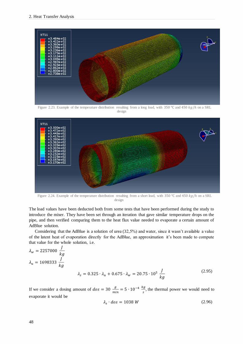
2. Heat Transfer Analysis

48

Figure 2.23. Example of the temperature distribution resulting from a long load, with 350 ℃ and 450 𝑘𝑔/ℎ on a SRL

design

Figure 2.24. Example of the temperature distribution resulting from a short load, with 350 ℃ and 450 𝑘𝑔/ℎ on a SRL

design

The load values have been deducted both from some tests that have been performed during the study to

introduce the mixer. They have been set through an iteration that gave similar temperature drops on the

pipe, and then verified comparing them to the heat flux value needed to evaporate a certain amount of

AdBlue solution.

Considering that the AdBlue is a solution of urea (32,5%) and water, since it wasn’t available a value

of the latent heat of evaporation directly for the AdBlue, an approximation it’s been made to compute

that value for the whole solution, i.e.

𝜆𝑤 = 2257000 𝐽

𝑘𝑔

𝜆𝑢 = 1698333 𝐽

𝑘𝑔

𝜆𝑠 = 0.325 ∙ 𝜆𝑢 + 0.675 ∙ 𝜆𝑤 = 20.75 ∙ 105

𝐽

𝑘𝑔

(2.95)

If we consider a dosing amount of 𝑑𝑜𝑠 = 30 𝑔

𝑚𝑖𝑛= 5 ∙ 10−4

𝑘𝑔

𝑠, the thermal power we would need to

evaporate it would be

𝜆𝑠 ∙ 𝑑𝑜𝑠 = 1038 𝑊 (2.96)

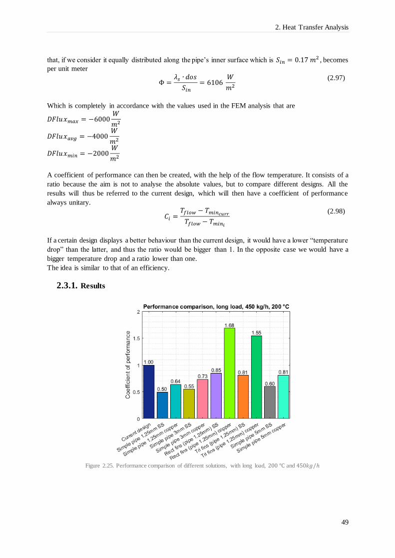
2. Heat Transfer Analysis

49

that, if we consider it equally distributed along the pipe’s inner surface which is 𝑆𝑖𝑛 = 0.17 𝑚2 , becomes

per unit meter

Φ =

𝜆𝑠 ∙ 𝑑𝑜𝑠

𝑆𝑖𝑛= 6106

𝑊

𝑚2

(2.97)

Which is completely in accordance with the values used in the FEM analysis that are

𝐷𝐹𝑙𝑢𝑥𝑚𝑎𝑥 = −6000𝑊

𝑚2

𝐷𝐹𝑙𝑢𝑥𝑎𝑣𝑔 = −4000𝑊

𝑚2

𝐷𝐹𝑙𝑢𝑥𝑚𝑖𝑛 = −2000𝑊

𝑚2

A coefficient of performance can then be created, with the help of the flow temperature. It consists of a

ratio because the aim is not to analyse the absolute values, but to compare different designs. All the

results will thus be referred to the current design, which will then have a coefficient of performance

always unitary.

𝐶𝑖 =

𝑇𝑓𝑙𝑜𝑤 − 𝑇𝑚𝑖𝑛𝑐𝑢𝑟𝑟

𝑇𝑓𝑙𝑜𝑤 − 𝑇𝑚𝑖𝑛𝑖

(2.98)

If a certain design displays a better behaviour than the current design, it would have a lower “temperature

drop” than the latter, and thus the ratio would be bigger than 1. In the opposite case we would have a

bigger temperature drop and a ratio lower than one.

The idea is similar to that of an efficiency.

2.3.1. Results

Figure 2.25. Performance comparison of different solutions, with long load, 200 ℃ and 450𝑘𝑔/ℎ

2. Heat Transfer Analysis

50

Figure 2.26. Performance comparison of different solutions, with short load, 200 ℃ and 450𝑘𝑔/ℎ

In the graphs few different behaviours can be observed.

First of all there is a substantial difference between the two different load conditions. In the short

load case, the fins seem to play a much bigger role with respect to the long load case, where the simple

pipe designs are closer to the current design result.

Nonetheless in the long load condition it should be considered that the longitudinal conduction

influence is greatly reduced, leading to a lower difference between the simple pipe designs (by varying

material and/or thickness) with respect to the short load case.

At the same time the finned designs present a different behaviour, showing bigger variations due to

material modification in the long load case.

This is rather strange since conduction appears to affect the configurations in different ways, whether

they are finned or not. However it is straightforward to understand that the result is a constant balance

between convection and conduction. In some cases, as it probably happens in the fins with the long load

case, the conduction can become a limiting factor, introducing big variations if modified.

Figure 2.27. Performance comparison of different solutions, with long load, 350 ℃ and 450𝑘𝑔/ℎ

2. Heat Transfer Analysis

51

Figure 2.28. Performance comparison of different solutions, with short load, 350 ℃ and 450𝑘𝑔/ℎ

Furthermore it is interesting to observe what happens if the mass flow is increased. If we look at the

same load conditions, the current design finned surface influence in general is slightly decreasing with

a higher mass flow. If we look for example at the simple pipe 1.25 mm thick, at 450 kg/h, 800 kg/h and

1850 kg/h it is clear how its performances are increasing with respect to the current design. This is

probably due to the fact that convection becomes less limiting on the overall heat exchange.

By looking at the results obtained with a limit value of 1850 kg/h (fig. 2.31), the 3mm copper simple

pipe performs even better than the current design.

Higher mass flow rates mean bigger convection coefficients, and therefore a generally smaller thermal

conduction influence in the overall performances, giving smaller differences between the simple pipe

designs.

Figure 2.29. Performance comparison of different solutions, with long load, 300 ℃ and 800𝑘𝑔/ℎ

2. Heat Transfer Analysis

52

Figure 2.30. Performance comparison of different solutions, with short load, 300 ℃ and 800𝑘𝑔/ℎ

Seeing the general better performances of the copper alloy, but being also incompatible with urea

environment, it’s been evaluated as interesting to simulate also a “sandwich” solution. It is basically a

pipe constituted by two layers, a thicker one made of copper and a thinner one made of stainless steel

(used just for protection).

If we assume a perfect contact between them, and therefore (almost) null contact resistance, the results

achieved for example with a layer of 1 𝑚𝑚 stainless steel over 3 𝑚𝑚 of copper differ of less than 1%

from the ones got with just a 3𝑚𝑚 copper pipe.

It is therefore of interest to investigate this solution further on.

Figure 2.31. Performance comparison of different solutions, with long load, 200 ℃ and 1850𝑘𝑔/ℎ

An analysis has been carried on also on the same designs using the convection coefficient that were

obtained by taking into account the mixer presence (fig. 2.33, 2.34).

2. Heat Transfer Analysis

53

Figure 2.32. Pipe detail with mixer (in violet)

As it happened for the higher mass flow rate, it introduces a bigger convection weight in the thermal

balance. Nevertheless the differences with the previous results are rather low, showing the same trend

as the “no mixer” analysis.

It should be considered that the mixer brings an increase in the outer finned surface convection but

at the same time a decrease in the convection on the inner surface (that can be a limiting factor in the

heat transfer).

Although the bigger convection leads to a lower conduction weight, and thus a smaller difference

brought by thickness variance in the simple pipe designs, it also results in a lower limiting effect

introduced by convection, causing a lower difference between the current design and the simple pipe

designs (comparing the 450 𝑘𝑔/ℎ, 200 ℃ with and without mixer). Nevertheless, theoretically a point

can be reached (and this is not the case) where the conduction becomes again highly important, and it is

when it becomes an unneglectable resistance in the radial heat transfer.

However, being the most critical conditions the ones with lower mass flow and temperature, we can

see that it doesn’t really make a difference to consider or not the mixer presence. That is why, together

with pursuit of simplicity, reducing the influencing variables number, in the following CFD calculations

and in the tests, the pressure drop introduced by the mixer won’t be considered.

2. Heat Transfer Analysis

54

Figure 2.33. Performance comparison of different solutions, with long load, 200 ℃ and 450𝑘𝑔/ℎ, considering the mixer

presence

Figure 2.34. Performance comparison of different solutions, with short load, 200 ℃ and 450𝑘𝑔/ℎ, considering the mixer

presence

2.3.2. Summary and discussions

To conclude, few considerations about this chapter can be made. Since the heat transfer coefficients

where deducted from the first theoretical model, they can be very different from the actual ones (their

correct evaluation will be made using a CFD tool in chap. 5). Nonetheless since in the CFD simulations

it won’t be possible to analyse the conduction influence on a un-homogeneous thermal load over the

pipe, the FEM were necessary to assess how beneficial can be an increase in thermal conductivity and

thickness.

2. Heat Transfer Analysis

55

Moreover, being the results highly dependent on the operating point analysed, it is rather complex to

come up with an optimum. In general it’s been pointed out how the thickness and the material thermal

conductivity are beneficial to the evaporation performances.

From this analysis it seems that a finned surface like the one currently used is particularly important at

low mass flow rates, while it becomes increasingly less effective at high flow rates. In addition with the

short load condition its influence is even more important.

A good solution, if possible, would hence be to use a slightly thicker pipe, coupled with simpler/less

fins, able to provide good convective heat exchange also at low mass flow rates.

57

3. Materials for exhaust systems

This chapter aims at considering different materials both to achieve better thermal performances and

lower costs. At the same time, having the component long life demands and being subject to harsh

environment conditions, its corrosion resistance must be kept at high levels.

The thermal performances will be analysed in terms of thermal conductivity, and the costs as raw

material costs. It should be anyway considered (as it will be done consequentially in the next chapter)

that softer materials, although having higher prices, could be simpler to manufacture, resulting in a lower

final component price.

Finally also the high temperatures typical of the exhaust systems, going up to 450 ℃ in this case, set

a requirement on the material to be suitable for the application.

3.1. Corrosion

Between all the species that could be formed inside the evaporator module, with the exception of NH3

that has been treated in chap. 1.6.2, it is possible to distinguish two acids, the isocyanic and the cyanuric,

which are both weak acids in aqueous solution, and that could create corrosion problems to the

evaporator pipe walls. This kind of corrosion is called wet corrosion and can result in different forms

such as crevice corrosion, erosion corrosion, galvanic corrosion, general corrosion, intergranular

corrosion (IGC), pitting corrosion, uniform corrosion and stress corrosion cracking (SCC). [25]

Together with wet corrosion, high temperature corrosion and especially oxidation, sulphidation,

carburization (due to CO/CO2), nitridation and attack by halogen gases can represent a risk for the

exposed surface. They are going to be quickly presented below.

It should anyway be always considered that temperatures brought to the exhaust system by hot exhaust

gases play a big role in all these processes. They definitely speed up these unwanted reactions, causing

some damaging risk to the pipe walls.

Both corrosion phenomena should then be taken into consideration when analysing the applicability

of different materials.

3.1.1. Carburization and nitridation

Basically carburization and nitridation consists in the precipitation of carbide or nitride (even in stainless

steels where Cr-Nitrides and Cr-Carbides precipitate), especially at the grain boundaries, which causes

a Cr pauperisation in the near zone, and consequently a weakening and a lower corrosion resistance of

the matrix. Usually these problems occur in atmospheres containing CO, hydrocarbons and nitrogen,

and this is particularly the case of exhaust gases. Nitridation therefore is very rapid in environments

containing ammonia, that is particularly the case of SCR systems [26, 9].

To be able to determine the susceptibility of materials to nitridation and carburization a key factor to

take into account is nitrogen/carbon solubility in the base metal.

3.1.2. Oxidation

Oxidation, being the most widespread high temperature corrosion reaction, consists of an oxides

formation from the interaction between the metal surface and oxygen. With the proceeding of the

reaction a thin layer that step by step increases in thickness is formed. It can be said that this happens

almost in every metal and alloy at high temperatures; is then the properties of this layer, as well as the

time needed to form it, that gives the material the corrosion resistance. If the layer is stable and compact,

3. Materials for exhaust systems

58

it can prevent the above material to come in contact with the oxygen, passivating the surface. In the

opposite case (with a brittle, porous layer which flakes off easily) the layer would keep on growing,

damaging the material.

The oxide, on a thermodynamic point of view, is formed when the potential pressure of the oxygen

in the environment is greater than the oxygen partial pressure in equilibrium with the oxide [24].

However, the kinetics of the process represents also an important variable. In fact, the process could be

so slow that no macroscopic effects would be appreciated during the whole components life.

The presence of water vapour it is well known to be detrimental on the high temperature corrosion

resistance of a lot of materials and for further insights about the reasons of this statement it is advisable

to check the related literature.

3.1.3. Sulphidation and attack by halogen gases

The sulphidation is a reaction similar to the oxidation but with sulphur instead of oxygen, and due to

both sulphur and metal characteristics is usually more aggressive than the above mentioned one. It

occurs with high temperature gases containing sulphur compounds, thus in our case with fuels

containing a trace of sulphur.

In the end halogen gases are dangerous for some materials since reacting with the metal they can

form highly corrosive species.

3.2. Stainless Steels

Exhaust systems are widely known for representing a harsh environment for the materials composing

them. This is due both to the high temperatures reached and the chemical species that could be found in

them. Nevertheless they need to fulfil strength and durability requirements.

Those demands have become more and more challenging over time, for marketing and emissions

legislations, causing the introduction of a new family of steels. After having used mild carbon steel for

this role for many decades, since 1990s stainless steels have become the primary material for exhaust

system’s components.

Stainless steel is a ferrous alloy, with chromium as most important alloy element. It has the beneficial

property of forming a stable and continuous layer made of chromic oxide (Cr2O3) that is able to protect

the underlying surface. This action is called passivation. The coating is addressed to be stable since its

grow rate is very slow, having the diffusion of cations through it as control mechanism. A minimum

amount of 11.5 % of chromium is required to form the continuous passivating layer, but with increasing

content better protections and therefore corrosion resistances can be achieved. The highest amount of

Cr that can be found in stainless steels is between 25 and 30% [11].

In addition to chromium a lot of other elements are usually added to the stainless steels, creating a

wide variety of them and differentiating their properties. A classification of stainless steels can thus be

made considering the different alloy elements and their structure. The five major families are :

Ferritic

Austenitic

Martensitic

Duplex

Precipitation hardened

In figure 3.1 it can be seen the famous Schaeffler diagram where the existing domains of the different

stainless steels typologies are plot function of Ni equivalent (austenite stabilizers) and Cr equivalent

(ferrite stabilizers) content in the material.

Stainless steels typical uses include railway, cars, trucks, processing of corrosive liquids, seawater

applications, chemical manufacturing, exhaust parts, heat exchanger parts, sinks, aerospace applications,

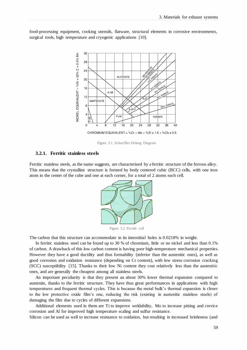
3. Materials for exhaust systems

59

food-processing equipment, cooking utensils, flatware, structural elements in corrosive environments,

surgical tools, high temperature and cryogenic applications [10].

Figure 3.1. Schaeffler-Delong Diagram

3.2.1. Ferritic stainless steels

Ferritic stainless steels, as the name suggests, are characterized by a ferritic structure of the ferrous alloy.

This means that the crystalline structure is formed by body centered cubic (BCC) cells, with one iron

atom in the center of the cube and one at each corner, for a total of 2 atoms each cell.

Figure 3.2. Ferritic cell

The carbon that this structure can accommodate in its interstitial holes is 0.0218% in weight.

In ferritic stainless steel can be found up to 30 % of chromium, little or no nickel and less than 0.1%

of carbon. A drawback of this low carbon content is having poor high-temperature mechanical properties.

However they have a good ductility and thus formability (inferior than the austenitic ones), as well as

good corrosion and oxidation resistance (depending on Cr content), with low stress corrosion cracking

(SCC) susceptibility [15]. Thanks to their low Ni content they cost relatively less than the austenitic

ones, and are generally the cheapest among all stainless steels.

An important peculiarity is that they present an about 30% lower thermal expansion compared to

austenite, thanks to the ferritic structure. They have thus great performances in applications with high

temperatures and frequent thermal cycles. This is because the metal bulk’s thermal expansion is closer

to the low protective oxide film’s one, reducing the risk (existing in austenitic stainless steels) of

damaging the film due to cycles of different expansions.

Additional elements used in them are Ti to improve weldability, Mo to increase pitting and crevice

corrosion and Al for improved high temperature scaling and sulfur resistance.

Silicon can be used as well to increase resistance to oxidation, but resulting in increased brittleness (and

3. Materials for exhaust systems

60

lower formability).

Ferritic stainless steels are designated, in the AISI standard, as 400 series.

3.2.2. Austenitic stainless steels

Austenitic stainless steels are contrariwise made of face centered cubic (FCC) cells, with bigger

interstitial holes and thus a greater capacity to store carbon atoms, up to 2.11 % in weight. Also the

atomic packing factor is higher, being slightly bigger in volume, but having 3 atoms of iron in each cell.

Figure 3.3. Austenitic cell

The most distinctive feature of austenitic stainless steels is the presence of high Nickel percentages,

from 6 to 22 % by weight. The chromium content varies between 16 to 27 % by weight [11].

Nickel is an austenite stabilizer particularly beneficial to mechanical properties and fabrications

characteristics; but also additional carbon can be used resulting in high strength (cork hardening), even

at high temperatures. This results in excellent ductility and formability. Furthermore nickel fosters

repassivation [12,13] and together with high chromium contents ensures excellent corrosion resistance.

Despite this, it’s been observed by Einar et al. [14] that they have quite high susceptibility to SCC

induced by chlorides. All these advantages however are hidden by a higher and fluctuating price due to

the high Nickel content, limiting a lot their applications.

The composition can be varied with Mo additions to increase resistance against chloric and reducing

acids and also to pitting corrosion. Ti and Nb additions, being efficient carbon binders, are used to to

reduce intergranular attack [12] and Si additions to increase scaling resistance. Mn and N [13] are

austenite stabilizers that can be used in substitution of some of the Nickel to reduce cost, giving also an

increment in pitting corrosion resistance [13].

They are designated, in the AISI standard, as 200 or 300 series.

3.2.3. Martensitic stainless steels

Martensitic crystal structure can be seen as obtained by a mechanical deformation of the austenitic cell,

to form a body centered tetragonal structure (BCT). Their peculiar characteristic is to have a high

quantity of carbon. This is not much beneficial to corrosion since it reduces its resistance to pitting

corrosion, crevice corrosion and intergranular corrosion. Nevertheless its high carbon content gives them

an excellent strength and hardness. Another problem with their application could be the higher

brittleness and lower weldability, brought by the high alloying with carbon.

The alloying elements that can be found are sulfur and selenium in order to increase machinability

and N, Ni and Mo (together with a carbon percentage reduction) in order to improve corrosion resistance

and toughness [13].

3.2.4. Duplex stainless steels

Duplex stainless steels contain both austenitic and ferritic phases in different balances between 40 and

50 %, with rather high molybdenum levels. This provides them a combination of austenitic and ferritic

3. Materials for exhaust systems

61

properties. Therefore they have great corrosion resistance as the austenitic ones and better cracking and

pitting corrosion resistance, thanks to molybdenum. They also present high mechanical strength,

toughness and good ductility (better than ferritic grades, but worse than austenitic grades).

The austenite stabilizers used are Ni, even though in much lower percentage with respect to austenitic

grades, and sometimes N. The latter improves also strength weldability and pitting corrosion resistance.

Thanks to the lower Nichel content, DSS represent a cost effective alternative to austenitic stainless

steels.

The big drawback with DSS is that their maximum allowed service temperature is around 300 ℃,

making them inappropriate for a lot of applications. As witnessed by Outokumpu after that temperature

embrittlement can be encountered [16].

3.2.5. Precipitation Hardened stainless steels

They are austenitic or martensitic stainless steels which thanks to added elements such as copper and

aluminium are subjected to precipitation of intermetallic compounds at aging temperatures. This results

in really high strength as well as good corrosion resistance, ductility and toughness. They basically reach

combined properties of martensitic and austenitic and are some of the most expensive stainless steels.

A wide table with all possible compositions of the most common stainless steel is presented in

Appendix C [17].

3.3. Stainless steels for evaporator pipe

For the evaporation pipe the three fundamental characteristics which the material should have are:

High corrosion resistance

High thermal conductivity

Price not too high

The first one, as discussed above, is because the silencer works in a quite harsh environment and

shouldn’t encounter big damages due to corrosion lifelong. Thermal conductivity is very important since

it increases the heat transfer between the outer annulus and the inner canal subjected to urea presence,

increasing its evaporation rate, as well as reducing the transients’ duration. In the end the price is always

a dominating variable in all engineering application, and especially in this project. Of course the final

component’s price is highly dependent on the manufacturing process used (available for that kind of

material), but in this case a first rough skimming will be done based also on the raw material prices

found.

Today’s version of the evaporator pipe in the large silencer is made of stainless steel 1.4509. That is

the same material used in most of the silencer components and this ensure a perfect compatibility both

for mountings and corrosion, since it has the same expansion coefficient and galvanic potential. It is a

ferritic stainless steel with the following composition.

Table 3.1 SS EN 1.4509 composition

EN AISI

C

(wt %)

Cr

(wt %)

Mn

(wt %)

Ni

(wt %)

Ti+Nb

(wt %)

Fe

(wt %)

1.4509 441 0,02 18 − − 0,6 𝐵𝑎𝑙.

As we can see it is stabilized both with titanium and niobium which reduce sensitivity for intergranular

corrosion, and the chromium content of about 18 % gives to it a good corrosion resistance and oxidation

resistance up to 950 ℃.

3. Materials for exhaust systems

62

It is suitable for welding with common methods applied to austenitic 300-series, has excellent deep-

drawability and it can be formed easily with typical forming processes. Its physical properties are listed

in table 3. Table 3.2 SS EN 1.4509 Physical properties [18]

Density 7,7 𝑔/𝑐𝑚3

Coefficient of thermal expansion 10 ∙ 10−6 1/𝐾

Thermal conductivity at 20 C 25 𝑊/(𝑚 ∙ 𝐾)

Modulus of elasticity 220 𝐺𝑃𝑎

Price 2 𝐸𝑢𝑟/𝑘𝑔

There have been some previous studies and tests of corrosion with urea involved, to emulate the material

behaviour upstream (evaporation pipe), in (catalyst) and downstream the SCR system. Urea and

ammonia give to the environment a more basic/alkaline characteristic. Urea’s pH is around 9-10.

Both ferritic and austenitic stainless steels corrosion performances have been studied and tested by

S. Saedlou and P. Santacreu [8] and R. Floyd et al. [9]. Although the austenitic have generally better

corrosion resistance, with a cost penalty, in this particular condition the ones analysed resulted to have

the same or even worse performances than the ferritic ones.

The earliest study of R. Floyd et al. [9] unveiled that even though at different exhaust temperatures

the materials have different relative performances (see Fig. 3.4-3.6), the most performing options across

all temperatures include 316Ti, 316L (austenitic) and 436, 444, 439 and 18CrCb (ferritic).

Figure 3.4. Results from the R. Floyd et al. tests at 300 ℃

Figure 3.5. Results from the R. Floyd et al. tests at 500 ℃

3. Materials for exhaust systems

63

Figure 3.6. Results from the R. Floyd et al. tests at 650 ℃

This is because different corrosion mechanisms intervene in the two different microstructures bringing

to similar performances. The best cost-effective solutions are thus without a doubt the ferritic ones and

in particular R. Floyd et al. selected 439 and 18CrCb. The test was conducted within a fume hood, with

a hot plate sprayed with urea from the injector. It had been done with constant duration, urea solution

and injector pulse width but with variable temperatures, injector frequency and materials. As can be

seen from the figures, also some coatings have been tested but they performed pretty bad in all the tests.

S. Saedlou and P. Santacreu [8] few years later investigated usual automotive grades to estimate

corrosion damage, with a different technique. In those tests, urea was injected on a plate subjected to

heat cycles of two types (a fast one of 2 min and a slow one of 1.5 hours) between the temperatures of

250 and 700 ℃. They also tested those materials with the addition of chlorides to simulate pollution

coming from fuel.

Figure 3.7. Total penetration of nitriding corrosion attack on laboratory simulation bench after 300h test (fast heat cycle) done by S. Saedlou and P. Santacreu [8]

3. Materials for exhaust systems

64

Figure 3.8. Influence of chloride pollutant on corrosion by urea decomposition products (fast heat cycle) from S. Saedlou and P. Santacreu’s study [8]

In both tests the two over-stabilized ferritics 1.4509 (441) and 1.4513 (436Ti) performed the best.

The selection of 1.4509 made for Scania’s silencers seems thus to be really accurate for corrosion, since

it is cost efficient and it doesn’t penalize the corrosion performances.

The stainless steels thermal properties are hence to be evaluated. As we can see from fig. 3.9, the

grade AISI 441 (1.4509), the orange dot, is between the best heat conductors and has also a reasonable

price, compared to all the stainless steels and especially the ones analysed above. The only ones that

have relatively better thermal conductivity are some martensitic grades, and the AISI 444 which, as it

has been said, could be a good alternative, slightly more expensive.

The martensitic ones are not considered to be good alternatives for this application since they have bad

weldability, as well as high hardness and they require more manufacturing energy.

Figure 3.9. Thermal conductivity vs Price for all stainless steel materials

3. Materials for exhaust systems

65

Austenitic stainless steel 304 grade (1.4301), which is known to be used by some competitor and was

used by Scania few years ago, although having a slightly lower thermal conductivity and a realtively

higher price can be justified if it allows to be manufactured with a cheaper manufacturing process, since

it is better formable and requires less processing energy.

3.4. Alternative materials

Given the importance of walls’ thermal conductivity it is worth considering the application of different

materials than stainless steels, with a better thermal conductivity.

If we analyse the thermal conductivity and the prices of all the materials families, it can be obtained

what is plotted in fig. 3.10, obtained using CES EduPack database [10]. In that graph it’s been chosen

to show all the available materials just for illustrative purpose. If the cost is limited to be under 50

EUR/kg and the conductivity higher than 20 W/m°C, a lot of them is automatically excluded.

Figure 3.10. Thermal conductivity vs Price for all materials commercially available

For example the materials with the highest thermal conductivity are diamond, silver, copper, gold and

aluminium. But diamond, silver and gold are unsuitable for this kind of engineering application and

aluminium is highly limited by its temperature performances. Furthermore, taking in consideration the

manufacturing processes suitable for each material, the necessity of compatibility within the complete

silencer (i.e. similar thermal expansion, etc.), and the service temperatures, it is easy to see that our

choice needs to be restricted to metals.

3. Materials for exhaust systems

66

Figure 3.11. Thermal conductivity vs Price for all metals

It has thus been plotted a chart (fig. 3.11) for all the metals with the following restrictions :

Price max 50 EUR/kg

Thermal conductivity min 20 W/m.°C

Maximum service temperature min 350 °C

Weak alkalis (7 < pH < 10) resistance : acceptable, excellent

Strong alkalis ( pH > 10) resistance : limited use, acceptable, excellent

Oxidation at 500 °C : limited use, acceptable, excellent

The green ellipsis represent the stainless steels already evaluated, as well as some carbon steel, cast iron

and tool steel. The carbon and tool steels are excluded due to their low corrosion performances while

the cast irons can be considered just in case casting would be evaluated as a promising process for the

manufacturing of the finned pipe.

As can be seen from the graph, the best trade-off between price, thermal conductivity, corrosion

resistance and workability is represented by the materials listed in table 3.3.

3. Materials for exhaust systems

67

Table 3.3. Comparison of the most promising materials

Thermal

conductivity

(W/m*C)

Max service

temperature

(C)

Price

(EUR/kg)

Density

(kg/m^3)

Weight

component

(kg)

Price

component

material

(EUR)

Copper Cr-Zr alloy

(C18100) 394 350 6,65 8940 3,40 22,60

Copper-chromium

alloy (C18200) 165 350 6,62 8940 3,40 22,52

Chromium,

commercial purity 89 490 8,71 7100 2,70 23,53

Bronze, CuAl10Fe5Ni5 42 360 6,37 7700 2,93 18,65

Nickel, commercial

purity 82 350 15,90 8880 3,38 53,72

Cu-2%TiB2 82,5 350 14,26 8780 3,34 47,62

Cast iron, austenitic,

EN GJLA XNiMn 13 7 40 475 2,43 7300 2,78 6,74

SS 1.4509 (AISI 441) 25 720 2 7700 2,93 5,86

SS 1.4301 (AISI 304) 17 835 3,44 7955 3,03 10,40

3.4.1. Cu-Cr-Zr alloy

The copper Cr-Zr alloy seems to be really convenient due to its really high thermal conductivity. It’s

approximately 17 times the one of the stainless steels used at the moment. Its great ductility can justify

also the higher raw material price.

However, its maximum service temperature, like the one of the majority of the other promising

materials, is rather low for the application. An explanation of what does maximum service temperature

mean is thus required. It is literally “the highest temperature at which material can be used for an

extended period without significant problems, such as oxidation, chemical change, excessive creep, loss

of strength or other primary property for which the material is normally used” [10].

Figure 3.12. Creep rates function of the applied stress for some copper alloys

3. Materials for exhaust systems

68

Figure 3.13. Strain trend with time for copper alloys exposed to a certain stress

Figure 3.14. Thermal conductivity as a function of temperature

The data about creep and yield strength found in fig. 3.12÷3.15, given also the low loads acting on the

pipe, show that the weakening effect after 350 ℃ is not too critical. The only issue to be solved is then

its oxidation and corrosion resistance in a urea environment. S. Saedlou et al [8] have observed that within the conditions found in the evaporator pipe, the

corrosion mechanism on stainless steels is mainly related to a nitriding/carbonitriding phenomenon of

the surface. Being much less the chrome quantity in the CuCrZr alloy, this effect it’s likely to not be of

great importance.

Copper in general has great corrosion resistance with unpolluted air, water and many saline solutions,

deaerated non oxidizing acids and many alkaline solutions. The corrosion products are usually protective.

For example some alloys can be subject, after some years, to the formation of a copper sulphate green

patina, which is an effective corrosion inhibitor [22].

However copper results also to be sensible to oxidizing acids, oxidizing salts, sulfur and most

importantly moist ammonia (NH3) and some NH3 compounds, as ammonium hydroxide solutions [22].

The best performing copper alloy in this environment is the Copper Nickel 30%, but having a lower

operating temperature limit and a much lower thermal conductivity (around 20 W/m∙C), is not advisable

for the application considered in this work.

To avoid then direct contact between CuCrZr and the urea environment, it could be of interest to

evaluate the use of a thin layer of the same stainless steel used nowadays (1.4509), or even better an

3. Materials for exhaust systems

69

austenitic one (AISI 304) which corrosion perfromances are well known and tested. The latter is thought

to be better for this use since it possesses a similar thermal expansion coefficient (17 ∙ 10−6 𝑠𝑡𝑟𝑎𝑖𝑛/℃)

to the CuCrZr alloy (16,8 ∙ 10−6 𝑠𝑡𝑟𝑎𝑖𝑛/℃).

Figure 3.15. Yield strength decrease with temperature

Nevertheless, oxidation is much more problematic given the high temperatures in play. This could be

solved by applying a high temperature silicon based ceramic coating (e.g. Thurmalox or Forrest Tech)

on the external surface of the pipe (the finned one), although the flanges could create an obstacle in the

application of the coating. If the thermal performances of a CuCrZr pipe are verified to be sufficient

without any heat flange, another stainless steel layer can be used also on the outer surface, leading to

the “sandwich” solution.

Furthermore, the galvanic corrosion that can start in the mountings (if they are connected to copper),

since could be really fast, has to be considered. Looking at the galvanic potentials in fig. 3.16 and from

CES edupack database [10] ferritic stainless steel 1.4509 has a galvanic potential between -0.14 and -

0.2 V while CuCrZr between -0.11 and -0.19 V, and thus really similar to the 1.4509 one. This means

that the galvanic corrosion happening in the interface between copper and the stainless steel mountings,

given also that the water presence in those areas is not continuous and poor, shouldn’t be too aggressive

[21].

A last aspect to take into account is the different thermal expansion coefficient (17 ∙ 10−6 𝑠𝑡𝑟𝑎𝑖𝑛/℃,

against 10 𝑠𝑡𝑟𝑎𝑖𝑛/℃ of the stainless steel 1.4509), which could bring to a redesign of the mountings in

order to allow a different expansion between the inner and the outer pipe.

Most common applications for this material are electrical (as circuit breakers, contacts, heat sinks,

switches and wires) and industrial (as continuous casting molds, fasteners, fusion energy targets, solar

collectors and resistance welding equipment) [23].

3. Materials for exhaust systems

70

Figure 3.16. Galvanic potential series in seawater

3.4.2. Chromium

Looking at his characteristics in table 3.3, commercial pure chromium appears to be a valid alternative.

Being slightly more expensive than copper alloys but having a lower density, it results in a final cost for

the component material approximately equal.

On the contrary instead it has a rather good maximum service temperature around 490 ℃. It is for

sure perfectly resistant to any kind of corrosion and oxidation and requires a little less (if soft) energy

than stainless steel to be processed. Its conductivity is around 89 W/m∙C and thus almost 4 times the

one of the stainless steel in use.

As said for the copper alloy, there could be problems with the mountings again. Chromium (with a

galvanic potential from -0.04 to -0.12 V) is more noble than stainless steel 1.4509 (-0.14 : -0.20 V), but

for the same reasons as before, it is sensible to suppose that this won’t be on a great scale. In addition,

chromium thermal expansion coefficient is 6 – 7 ∙ 10−6 strain/C, different from the outer pipe’s one

(10 ∙ 10−6 strain/C).

What makes chromium unsuitable for applications different than protective coatings and alloying

element is its toxicity. Even though just chromium VI compound is highly toxic and carcinogenic, all

chromium compounds should be considered toxic and polluting.

Typical uses are protective coatings, as alloying element in steel and superalloys and as catalyst [10].

3. Materials for exhaust systems

71

3.4.3. Nickel

Nickel, although being far more expensive, is extremely easy to manufacture and possesses a

conductivity of more than 3 times the 1.4509 grade’s one. However at the same time it has both a low

strength and a rather low maximum service temperature.

Despite of this it has an excellent corrosion resistance, thus it could be considered as an alternative

only if the material price is not too influencing on the final component cost (balanced by the cheap

manufacturing process) and the low yield strength (around 100 MPa at 26,9 ℃) doesn’t allow large

deformations. Creep phenomena could be dangerous with this material.

Nickel’s galvanic potential around -0,20 : -0,25 V doesn’t appear to be too critical together with

stainless steel.

Common nickel applications are cathode shanks, fluorescent lamps, electrodes, heat exchangers and

heat shields [10].

3.4.4. Others

The Cu-2%TiB2 in addition of being more expensive has the same issues about temperatures and

corrosion and has lower ductility than CuCrZr alloy. Furthermore its much lower conductivity makes it

not preferable than the last mentioned one.

The bronze has an almost twice higher conductivity than 1.4509, but 3 times higher price as well as

lower ductility and lower maximum service temperature. It is therefore not desirable to be used instead

of the used stainless steel.

And finally the cast iron could be interesting just if casting represents a suitable technique for the

manufacturing of the component. These material proposals, before being implemented, need without any doubt to be investigated more

deeply and accurately, with possibly some actual testing, especially for the corrosion performances.

3.5. Summary

Completely different materials have been considered in this chapter, and evaluated in terms of :

- Price

- Thermal conductivity

- Corrosion resistance

- Maximum service temperature

Their characteristics are summed up in table 3.4.

3. Materials for exhaust systems

72

Table 3.4. Summary of the material analysis

Material Advantages Disadvantages

CuCrZr alloy - Extremely high thermal

conductivity

- Great workability

- Price not too high

- Low maximum service

temperature

- Poor corrosion performance,

especially with urea

Chromium - Good thermal conductivity

- Good maximum service

temperature

- More ductile than stainless

steel

- Great corrosion resistance

- Can be toxic

- Slightly more expensive than

CuCrZr alloy

- No applications different than

protective coatings

Nickel - Easy to manufacture

- Good thermal conductivity

- Excellent corrosion resistance

- Very expensive

- Low strength

- Low maximum service

temperature

Cu-2%TiB2 - High thermal conductivity

- Good ductility

- Price not too high

- Very expensive

- Low maximum service

temperature

- Poor corrosion performance,

especially with urea

- Lower thermal conductivity than

CuCrZr alloy

Bronze - Better thermal conductivity

than SS 1.4509

- Better corrosion resistance

than previous copper alloys

- Price not too high

- Low ductility

- Low maximum service

temperature

- Lower thermal conductivity than

CuCrZr alloy

- Same price as CuCrZr alloy and

Cast iron - Low price

- Better thermal conductivity

than SS 1.4509

- High maximum service

temperature

- Lower corrosion resistance than

stainless steels

- Can only be casted

SS 1.4509 - Extremely low price

- Good corrosion resistance

- High maximum service

temperature

- Low thermal conductivity

- Low ductility

SS 1.4301 - Low price

- Very good corrosion resistance

- High maximum service

temperature

- Higher price than SS 1.4509

- Lower thermal conductivity than

SS.14509

- Low ductility

73

4. Manufacturing processes

In this chapter the manufacturing processes that can be used to produce the evaporation pipe are going

to be assessed. After presenting the ones used for all Scania silencers, a quick review of the relevant

techniques, with advantages and drawbacks for the application will be done.

In addition to cost saving, also simplicity and flexibility are important, because it means more supplier

would be able to manufacture it, opening more possibilities for the company.

The manufacturing processes available nowadays are many and variegated. They can be divided in

few big classes, each one representing the theoretical common base of a group of processes. They are :

Forming (sec. 4.2)

Casting (sec. 4.5)

Machining/Cutting (sec. 4.6)

Additive Manufacturing/Rapid Prototyping

Powder methods

Welding/Brazing

Each large class is then formed by processes in some case very different one from each other.

In this thesis anyway it is going to be presented a quick description of the ones that can be of interest

for the AdBlue evaporator finned pipe production.

4.1. Manufacturing processes used for Scania’s evaporation units

4.1.1. Large silencer

The manufacturing process currently used for the large silencer’s evaporation module (used with V8

Scania engines) consists of a two steps process.

First the pipe is created from a sheet of stainless steel 1.4509, 1.25 mm thick, bended and welded at

its lateral limits. Afterwards, another sheet made of the same material but thinner (0.2 mm) is folded to

model the particular rectangular shape of the flanges, and then laser welded in the centre of their bases.

This of course appear as an expensive procedure to be carried on, and it is indeed. It is sufficient to

mention that to automate the welding, a robot cell has been developed that after each welded line, shifts

angularly the pipe to identify a new area that needs to be welded. Furthermore, giving that the number

of longitudinal flanges is approximately 144, and that the finned length of the pipe is 0.355 m, we can

easily compute that 51.12 m of welding are needed.

All those different operations needed increase the component cost a lot, which for the serial

production required by Scania and their suppliers is estimated roughly around 40 euros. This is another

reason for this work; different manufacturing processes with different materials are going to be evaluated,

to find the best trade-off between cost and performances. Simplifying the currently used process, is also

beneficial because it allows more supplier to be able to manufacture the evaporation unit and therefore

both more flexibility and lower prices brought by the competition between the different suppliers.

We can start by analysing the other solutions adopted on the evaporation modules of different silencer

sizes, i.e. medium and common.

4.1.2. Medium silencer

The medium silencer is used with smaller engines and it’s characterized by a smaller evaporation unit.

It can be found in two different configurations, respectively for high and low power engines, and they

4. Manufacturing processes

74

differ one from the other just from the presence of flanges on the outer surface. Their design, different

from the larger one, consists of a complex geometry, both on the inside, and the outside (where the

flanges are positioned) of the terminal part of the inner pipe.

This makes it advantageous to directly cast it (with the same material of the larger one, i.e. stainless

steel 1.4317) in one piece. After that it needs to be machined on the inside, to finish the surface and

avoid areas beneficial to deposits build-up. The more the surface is smooth, the easier the urea droplets

slip on it and prevent build-ups.

As opposed to the previous manufacturing method discussed, this process, standardized, is slightly

cheaper and easier to realize. But it could be used just because less flanges are needed and thus less

accurate.

4.1.3. Common silencer

The common silencer has not an evaporation pipe, but instead the urea doser directly sprays urea against

the silencer walls. This evaporation chamber is not effective as the other two ones and so this silencer

can’t reach Euro 6 regulations. It is however still used in some applications in other countries where

earlier Euro regulations (Euro 5 and lower) are still applying, as for example trucks for Brasil.

4.2. Forming

The base concept of forming manufacturing processes is the plastic deformation of the processed

material, in a solid state. That is highly limiting the obtainable shapes, with respect for example to

casting, and is the reason why plastic deformation mechanism in the material is really important to

understand the different behaviours and the forces occurring.

There are two different forming typologies, cold forming and hot forming, and each of them has

different deformation mechanisms.

In cold forming processes (low temperatures compared to material’s melting temperature), the

predominant mechanism is the slip between atomic planes, which is influenced by the interatomic

distance and the inter-planar distance. This slip is highly affected also by the presence of dislocations,

and Orowan discovered in 1934 that plastic deformation could be explained with the theory of

dislocations. During cold working metals undergo to dislocation formation that results in a dislocation

density increase. They gradually create strain fields of different magnitude overlapping one to each other

and hence increasing material resistance to deformation. This phenomenon is called strain hardening.

It is the reason for the increasing stress-strain curve trend and means that the consequences of cold

forming are an increase in yield strength, in traction resistance and a decrease in formability.

As a matter of fact, to achieve a great deformation with cold forming, many steps are needed, both to

reduce the pressure and wear on the tools and to avoid damages to the material. Later thermal treatments

(as annealing) to reduce strain hardening effects are usually needed.

The advantage of cold forming are the better surface finish and dimensional precision (tolerance)

achieved, no energy for heating, low tool material costs and increased component strength.

Hot forming instead is performed at high temperatures, above the recrystallization temperature.

Dislocations can move more easily and this results in a lower strain hardening effect. In addition the

temperature brings with it a dynamic recovery which creates a softening of the material.

The dominating mechanism is thus dependent on temperature, strain rate and crystal structure.

The advantages of hot forming are thus a smaller force and power required, bigger deformations and

more complex shapes achievable, due to material’s ductility.

The principal forming processes are:

Forging and pressing

Sheet metal forming (deep drawing, bending, metal spinning, etc.)

Rolling

4. Manufacturing processes

75

Upsetting

Extrusion and wire drawing

Each of them has then many variants but in the following just the interesting processes (for the

evaporation pipe) are going to be analysed.

4.2.1. Stresses analysis

The parameters of interest to study the stress/strain in a process which involves plastic deformation are

the true stress and the true strain. This is because, in the big strains field, they are much closer to the

physical reality of the phenomenon. They are defined :

𝜎 =

𝑃

𝐴

(4.1)

휀 = ∫

𝑑𝑙

𝑙

𝑙

𝑙0

= ln𝑙

𝑙0= ln

𝐴0

𝐴

(4.2)

The tensile test is the simplest material deformation example, and looking at its stress-strain curve,

you can have an idea of the material behaviour in terms of resistance to formability. The estimated law

for the stress-strain curve is :

𝜎 = 𝐾 ∙ 휀𝛽 (4.3)

Where K and 𝛽 are two variables, respectively the strength coefficient and the strain-hardening

coefficient, characteristic of the material. In table 4.1 and fig. 4.1 can be found as an example some

values from different steels and other selected materials at room temperature.

Table 4.1. Values of strength coefficient and strain-hardening coefficient for some common materials [28]

Material K (MPa) 𝜷

38CrMo4 750 0.08

17NiCrMo7 650 0.15

100Cr6 1475 0.07

X15CrNi1808 1300 0.30

X15Cr13 970 0.10

304 stainless steel (annealed) 1400 0.43

Copper (annealed) 530 0.44

4. Manufacturing processes

76

Figure 4.1. Stress-strain curve using the data from table 1 for different materials

The work required for a deformation per volume unit, being

𝑊𝑖 = ∫ 𝜎 ∙ 𝑑휀

1

0

(4.4)

it can be seen as the area underlying a stress-strain curve.

By using equation 4.3 it can be obtained

𝑊𝑖 = 𝐾 ∙

휀𝛽+1

(𝛽 + 1)

(4.5)

It is thus important to evaluate the deformation and then the strain work, since it can be used to evaluate

the forces involved in the process by equalizing the work done by external forces and the energy required

by the deformation.

Furthermore, especially in hot forming, the strain rate is highly influencing the deformation and the

flow stress, which represents the stress value required to start and maintain the plastic deformation (after

having reached the yield strength). This is because of the contention between the recovery and the strain-

hardening in action. The expression used to evaluate the flow stress, function of the strain rate, is:

𝜎𝑓 = 𝐽 ∙ 휀̇𝛾 (4.6)

Again the coefficients depending on the material, as well as the deformation and the temperature value.

Some examples can be found in table 4.2.

Table 4.2. Examples of values for the coefficients useful for the flow stress evaluation [28]

Material Temperature (C) J (MPa) 𝜸

Al alloys 200-500 300-40 0.05-0.02

Cu alloys 200-800 400-20 0.02-0.3

Low %C steels 900-1200 170-50 0.08-0.20

Stainless steels 600-1200 420-40 0.02-0.4

4. Manufacturing processes

77

Figure 4.2. Graphical representation of the values from table 4.5 for copper alloys (blue line) and stainless steels (red

line)

Figure 4.3. Experimental curves with different strain rates 휀̇1 < 휀̇2 < 휀̇3 < 휀̇4

It can be clearly seen from figure 4.3 that the higher the strain rate, the higher the strain-hardening effect

(since less time is available for the recovery) and thus the higher the stress required to deform the

material.

So far it has been considered just a mono-dimensional stress state, even though in every

manufacturing process the state of stress is three-dimensional. A general 3-dimensional state of stress

can always be broken down into a deviatoric and a hydrostatic portion, and three perpendicular planes

can always be defined, where all the shear components are equal to zero. They’re called principal planes

and the normal stresses existing on them are named principal stresses.

In order to compare the 3-dimensional state of stress to the yield strength (which is basically a value

from a one dimensional tensile test), three yield criterion have been developed, with the aim of

synthesizing the state of stress in a 1-dimensional one. They are, in a chronological order, Galileo,

Tresca and Von Mises criterion, and each one is best suited on a particular family of materials. For

further insights it is advisable to read the relative literature [28,29].

4. Manufacturing processes

78

4.2.2. Formability

Formability refers to the capacity of a metallic material to withstand deformations without damages. It

is dependent on different parameters stated below [29] :

Workpiece material - Highly influencing. Condition resulting from chemical composition,

material’s microstructure, heat treatment and process steps.

Workpiece temperature - Affects the balance between recovery/recrystallization and strain-

hardening. The higher the temperature, the higher the formability

Forming rate - Affects the tendency to brittle fracture. Generally the higher the forming rate,

the lower the formability.

Stress state in the workpiece – The hydrostatic component of the stress (𝜎𝑚 ) has a large

influence on material formability. The lower it is, the higher the formability is (with 𝜎2 =

𝑐𝑜𝑛𝑠𝑡 ).

Figure 4.4. Effect of stress state on formability [30]

In order to express the deformability of a material as a characteristic value, different damages criteria

have been developed. They can be time-dependent and time-independent and macromechanical and

micromechanical [29]. From the combination of those 4 different criteria comes out the final evaluation

and they are used as fundamentals to assess material deformability in most FEM programs.

Forming Limit

On the other hand, forming can be limited by process-specific parameters. In most of cases they are:

Tool fracture

Insufficient machine power

Shape and dimension achievable

Required surface quality

Depending on the material and on the application, forming is restricted by the most critic between

formability and forming limit.

4.2.3. Materials in forming

The general characteristics that are always beneficial for components forming are [29]:

Minimal flow stress

Low strain-hardening effect

Homogeneous rain structure along the initial cross-section

4. Manufacturing processes

79

High formability

A classification of different materials can then be made with increasing flow stress [29]:

I. Lead and lead alloys

II. Tin and tin alloys

III. Aluminium and aluminium alloys

IV. Zinc and zinc alloys

V. Copper and copper alloys

VI. Unalloyed and alloyed steels up to about 0.45% C (in annealed state)

VII. Corrosion-resistant ferritic and martensitic Cr steels

VIII. Austenitic CrNi steels

IX. Nickel and nickel alloys in a solution-annealed state

X. Titanium and titanium alloys

The most interesting groups for the AdBlue evaporator application, as stated in chapter 3, that are

going to be discussed are Copper and copper alloys, Ferritic, Martensitic and Austenitic stainless steels

and Nickel and nickel alloys.

Copper and copper alloys.

Thanks to their wide applications fields and their high deformability in the cold state they are important

materials for cold forming parts. Especially pure copper (with percentage between 99.5 and 99.9 % of

Cu [31]) is the one with the highest formability and with it solid and hollow profiles of the most varied

cross-sections can be achieved. Mechanical properties change with cold forming of electrolytic copper

are presented in fig.4.5.

Figure 4.5. Mechanical properties (Rm, Rp02 and A) change with elongation for electrolyte copper [31, 32]

Another important copper alloy material, having a share of 70 % of all the copper alloys production [34],

is the copper-zinc alloy (Brass) but it will not be described since it is not of interest in this case, due to

its low maximum service temperature (around 200 ℃).

Stainless steels

Cold forming application of stainless steels are increasing since it allows the usage less material, leading

to cost savings (the prices of this family are higher than normal steels), and also because often stainless

steels are not prone to machining (due to tool wear and bad chip shape).

4. Manufacturing processes

80

In general steels have high strength, resulting in harder cold forming and special microstructure

requirements. Their formability is highly dependent on alloying elements. E.g. high carbon content is

particularly detrimental to formability, since it could lead to carbides and unfavourable microstructures.

Figure 4.6. Flow stress vs True strain for three different steels [29].

In fig. 4.6 are showed the behaviours of 3 different steels. It can be clearly seen the different trend of

the austenitic stainless steel (X5CrNi 19-11), due to a higher strain-hardening exponent. This is rather

different from a ferritic one and makes it necessary to adjust the blanks with respect to the deformation

it is undergoing during the forming process.

Nickel and nickel alloys

Due to material saving and the nickel’s high price, as well as difficult machining, cold forming of nickel

alloys is of great economical interest. Materials with more than 99,5 % of nickel are the easiest to cold

form, and even without intermediate annealing they can achieve high degrees of deformations up to

extreme ones with intermediate annealing.

Pure nickel alloys, having similar properties as steel with 0.2% C [33] in the field of comparable

deformations, have the same problems of increasing mechanical properties and forces required with

deformation, fig.4.7.

Figure 4.7. Hardness increase during cold forming of different materials [33]

4. Manufacturing processes

81

4.2.4. Hot forming

Hot forming basically is used to increase formability, reduce flow stress and thus the forces involved in

the process. Even though all formable materials should be suitable for this process, the most common

and of interest are steels above all and then magnesium, aluminium, titanium, copper, and nickel.

The most important parameter in this process is the temperature, since it is based on a trade-off

between recovery/recrystallization and strain-hardening. Furthermore it should be considered the

thermal stresses which the components and the tools are subjected to, and that can in the worst case

cause fractures.

Lange [35] made a ranking of materials suitable for hot forming, from the best to the worst one :

I. Aluminium alloys

II. Magnesium alloys

III. Copper alloys

IV. Carbon steels, alloyed steels

V. Martensite-hardening steels

VI. Austenitic stainless steels

VII. Nickel alloys

VIII. Titanium alloys

IX. Iron-based superalloys

X. Cobalt-based superalloys

XI. Molybdenum alloys

XII. Nickel-based superalloys

XIII. Tungsten alloys

XIV. Beryllium

4. Manufacturing processes

82

4.3. Extrusion

Extrusion is a process used to create objects by pushing with a ram through a shaped die a billet to whom

is thus given a desired cross-section. In the tube extrusion case a mandrel is placed in the middle of the

die. It is a process used in the production of a great variety of sections including tubing, bars, window

frames, buildings and automotive trim, aircraft structural parts, railings and so on. Its advantages are the

possibility to create very complex sections, to allow great deformations (smaller for brittle materials)

thanks to a compressive stress state generated in the process, and to guarantee an excellent surface finish

of the part (especially with cold extrusion).

There exist different extrusion processes, depending on the tool type (rigid tools or active media),

the direction of material flow relative to the ram direction (forward, backward or lateral), and the shape

of the final workpiece (solid, hollow, cup).

Figure 4.8. Direct and indirect extrusion (left) and hydrostatic extrusion (right)

The difference in tool type is between a punch and a fluid pressurized by a forming press or a pump;

this kind of extrusion is called hydrostatic extrusion. The active medium, surrounding the workpiece on

all sides, allows a better formability, since the crack opening occurs at higher true strains, as well as a

lower friction. For process related reasons the hydrostatic extrusion can be only of a forward type.

Furthermore forward and backward extrusion (called also respectively direct and indirect), the most

common ones, in addition to the hollow shaped ram in the latter, differ a lot in terms of extrusion forces

required. This is due to the friction between the billet and the container. In the case of indirect extrusion

the relative motion between them is absent, resulting in a smaller friction force and thus a smaller global

extrusion force (fig. 4.9).

Figure 4.9. Force trend function of ram displacement with different types of extrusion

In order to overcome this problem, especially with steels, a lubricant with a good high temperature

viscosity is often used. The common ones are glass and graphite.

4. Manufacturing processes

83

Being easier in terms of forces and power requirements with the same deformation, hot extrusion is

used in most cases, which means working temperatures around 70-90 % [36] of the melting temperature.

Common working temperatures for aluminium alloys are between 400-500 °C, 900-1300 °C for steels

and 650-1000 °C for copper alloys.

Anyway, if a higher accuracy is required cold extrusion is needed, and usually more than one step.

Achievable accuracy depends on shape, material, steps breakdown, tool condition, process control and

heat treatments. A comparison between accuracies characteristic of different methods can be seen in fig.

4.10. Many other errors and defects anyway can be obtained with this process, if not designed carefully.

Figure 4.10. Manufacturing methods achievable accuracy

Table 4.3 lists surface qualities achievable in case materials, lubricants, and shaping tools used are the

proper ones.

Table 4.3. Roughness values for extrusion process

Process Surface Roughness Ra

Inner wall (𝝁𝒎) Outer wall (𝝁𝒎)

Cup backward extrusion 1-3 1-2

(long measuring length) - 8-20

Steel forward extrusion 2-3 3-4

(long measuring length) 6-9 8-15

Extrusion is a stationary process, i.e. the force applied on the punch is almost constant all the process

long, and discrete, i.e. the billet needs to be loaded for each extrusion/component extruded.

As already mentioned in section 4.2, different parameters affect the forming process, as material

properties, the process itself, the tools’ loading capacity and the available machine power. Even though

the material is attributed to be of greatest importance, other constraints can limit materials formability.

They can be for example flow hindrances related to geometry, friction phenomena at workpiece-tool

interface or accuracy requirements.

Table 4.4 can be used as a reference for limiting strain values for different materials.

4. Manufacturing processes

84

Table 4.4. Limiting strain in cold extrusion for different materials [29]

Material Forward extrusion Backward extrusion

𝛗𝐯𝐦𝐚𝐱 |𝛆𝐀|/% 𝛗𝐯𝐦𝐚𝐱 |𝛆𝐀|/%

Al 99.5, AlMg 1, AlMg 3, AlMg 5, AlMgSi

0.5, AlMgSi 1

3.0-5.0 95-99 2.5-4.5 90-98

AlCuMg 0.5, AlCuMg 1

2.5-3.0 90-95 1.4-1.8 70-85

E-Cu 99.9 R-Cu 99.5, CuZn 37, CuZn 28

1.4-2.0 70-85 1.4-1.6 70-80

C 2 E, C 4 C

2.2-3.0 85-95 1.4-1.8 70-85

C 10 C, C 10 E, C10

1.6-2.0 80-85 1.4-1.6 75-80

C 15 C, C 15 E, C15

1.4-1.6 70-80 1.1-1.3 65-70

C 22 C, C 22 E, C 25 E, C25, C 35 C, C 35

E, C 35

0.8-1.0 55-65 0.7-0.8 50-60

15 Cr 3, 15 CrNi 6, 16 MnCr 5, 20 MnCr 5 0.7-1.1 50-67 0.5-0.8 40-65

34 CrMo 4, 41 Cr 4, c45, 42 CrMo 4, 25

CrMo 4

0.5-0.6 40-45 0.5-0.8 40-55

4.3.1. Economic investigation

Extrusion is potentially competing with other manufacturing methods, that are machining, electric

discharge machining, casting, forging and sintering.

Economic criteria used for the comparison are:

- Saving on material

- Reduction of manufacturing time

- Better mechanical properties of the final product

Excluding casting and forging since they won’t provide a finished product, the two competitors that

need to be evaluated are extrusion and machining.

In machining the scrapped volume is usually pretty high, up to 56% of the initial volume [29], while

in extrusion it is only around 1%. This results, especially with expensive materials, in a high saving on

material cost. Moreover, the favourable orientation of the grain structure which has been subjected to

forming gives the component a better strength plus being affected by strain-hardening during the process.

Extrusion due to tool life and short set-up times is also faster, having a productivity up to 60 parts per

minute i.e. almost 10 times higher than machining with numerical control for parts with simple

geometries [29]. But one of the biggest advantages is that, thanks to the increase in accuracy achievable

with forming, it can be seen as almost a single operation competing with other manufacturing sequences,

as the one needed for machining.

In table 4.5. there can be found guide values for minimum numbers of parts for a convenient extrusion

manufacturing application, depending on the weight of the part, and thus the material quantity used.

They are reliable for steel components and complex ones made of non-ferrous metals.

Table 4.5. Minimal economic lot size for steel cold extrusion [38]

Weight per part

(mass in g)

Minimum size of lots

(parts)

Weight per part

(mass in kg)

Minimum size of lots

(parts)

<10 200,000 1-3 5,000

10-100 100,000 3-5 2,000

4. Manufacturing processes

85

100-250 50,000 5-10 1,000

250-500 25,000 >10 500

500-1000 10,000

Table 4.6. presents a comparison of costs detail of the total cost, expressed as ratios between the

different processes, with warm extrusion and close-tolerance forging as reference. It should anyway be

considered the difference in accuracy between the methods.

Table 4.6. Ratios representative of cost shares for different methods [35]

Cost shares Cold

extrusion

Warm extrusion,

close-tolerance

forging

Closed-die

forging

Material costs 0.80 1.00 1.00

Tool costs (original production) 1.10 1.00 0.70

Tool costs (maintenance) 0.70 1.00 1.30

Costs for surface and heat treatment 2.00 1.00 1.00

Machine costs 1.20 1.00 0.90

Total 5.8 5 4.9

As a conclusion, extrusion results to be a very interesting process, especially for high-volume

production (fig. 4.11) of rather simple components, not requiring too low tolerances.

Figure 4.11. Comparison between machining and forming in manufacturing costs for a simple component [36]

For a shape like the evaporation pipe however it must be considered that machining is not a solution to

consider because it would involve an extremely long process, especially with stainless steel which is not

really suitable for machining.

Scania’s large silencer request is around 10000 units/year, and therefore extrusion application seems

to be rather convenient for the evaporation pipe if it was possible to avoid post-process machining on

the inner surface.

Nonetheless stainless steel requires really high extrusion forces and in order to obtain a shape as needed

has to be hot extruded. This means that there would be a limit in the achievable pipe’s thickness as well

as in the fins width and overall tolerances and roughness. There have been discussions with Sandvik,

which is a world leader in materials technology, and the rough limit in thickness that can be reached

with stainless steel extrusion has been evaluated to be 3 𝑚𝑚. Furthermore it would need a machining

on the inner surface to get a good surface finishing.

This makes the extrusion idea not the best cost-efficient one for stainless steel. But as it’s been

demonstrated above copper, having a much better formability, can be extruded easier, and therefore it

could be probably extruded with a cold extrusion process. This is another strong reason of considering

its application in this context. For sure, since nothing similar has ever been done earlier, a further study

with some FEM simulation as well as testing needs to be carried on.

4. Manufacturing processes

86

4.4. Cold forming pipe’s manufacturing

A solution that according to Sandvik expertise can be feasible is by giving the desired shape to the pipe

with some incremental steps of cold-forming. In this way, less than 3 𝑚𝑚 thicknesses of both pipe and

flanges can be reached. Good flanges heights and good surface finishing are also possible to obtain

without requiring a too big effort. This means that the machining afterwards can be avoided, representing

then a good cost-effective alternative.

The challenge with this technique is the fins shape and quantity. It is straightforward to see that the

dimensions of the current design can’t be realized but a good compromise that maybe penalizes a bit of

convection but results in a better conduction, reaching the same performances with a lower end-item

cost, can be definitely found.

4. Manufacturing processes

87

4.5. Casting

Taking inspiration from the evaporation module in the medium silencer, casting should be evaluated

since if it is able to produce the right geometry (tolerances and roughness required) without defects and

without requiring too much post-processing (machining usually) it could be very cheap.

It consists of liquid metal poured into a mould previously shaped with the desired geometry, where

it solidifies and is then either ejected or broken out of the mould (single use mould).

The mould can be permanent, and so used for a lot of castings, or expendable, used for few or even just

one casting. Between these two classes, a lot of different methods stand out. They differ for mould’s

material, such as sand or metal, as well as for pouring strategy (pressure, gravity, etc.) and so on. In fig.

4.12 an overview of the casting methods is showed.

Figure 4.12. Casting methods overview

The fundamental casting with expendable moulds (the most common material is sand) system include:

- Pouring basin

- Sprue

- Runner

- Core

- Riser

- Flask

- Gating system

- Division plane

The challenges related with this process are the extractability of the parts without damaging the mould

and thus some geometry limitations on the achievable shapes; the metal solidification and the possible

defects related to that; the workpiece tolerances achievable as well as the surface finish; the need of

machining after that.

As can be seen from fig. 4.10 the accuracy achievable with precision casting is between IT11 and

IT14. The average surface roughness is between 6.3 and 0.8 𝜇m for permanent mould casting and 3.2-

0.8 𝜇m for investment casting and die casting. The lower values can be achieved only with special

processes [40]. This means that the process is rather coarse and a machining is commonly needed to

achieve the precisions require in the final product.

This is particularly the case of the evaporation pipe. As witnessed by the medium silencer version, with

its casted part, a machining/finishing is mandatory on the inner surface, where urea hits the walls, in

order to remove favourable areas for deposits build up. On the other hand for the outer surface, not

4. Manufacturing processes

88

having surface roughness requirements, the only critical factor is the tolerances on the fins dimensions

and their shape.

Draft angles and smooth fillets are introduced to help the extraction. Shrinkage (that could be either

in a liquid or a solid phase) requires one or more sprues and an accurate design of the shape is needed

in order to allow directional solidification and avoid defects or discontinuities in the workpiece. The

most common ones are shrinkage defects, gas porosities, misruns, cold shuts, inclusions, hot tears and

hot spots. Another thing to be considered is the oversizing in order to leave material for the surface final

machining. Its dimensioning depends on different parameters such as the part dimensions, the casted

material, the surface quality required and the kind of casting method used.

Permanent moulds, being made of metal and having a higher conductivity, avoid the formation of

big dendrites (typical of sand casting) bringing thus to a fine crystalline structure and better mechanical

properties. In addition the granulometry and imperfections/deformations common in expendable moulds

are missing bringing to a high quality both in surface finish and dimensional tolerances, and most

important constant during the whole production. Being the metal mould not porous on the contrary

some vent channels are needed to let the air and gases go out of the mould before the solidificat ion.

This advantages anyway are counterbalanced by a higher tool cost, making this technique cheap just for

big production lots.

Materials in casting processes play an important role. They need to have a high fluidity and a low

viscosity to ensure a high castability. Common foundry alloys suitable for permanent casting are light

alloys, copper alloys, zinc alloys, white anti-friction alloys and some cast irons.

For the large silencer’s shape anyway this method doesn’t seem to be appropriate, since the

component and thus the fins are pretty long, leading to a high reduction in height due to the necessary

draft angle. In fact, if the split plane is at half the length there would be 0.1775 m on each side and with

for example 2 degrees of draft angle, means a height reduction of 6.2 mm, almost the height used in the

current design.

The only casting method able to allow zero or even negative draft angles as well as good surface

finish and good accuracy is the so called investment casting. This process has an old origin, with the

lost-wax casting. Although the materials used to create the patterns have changed, the concept is still

the same. After the production of the master die the patterns can be manufactured, and in some cases

assembled in multiple patterns. The materials used nowadays for the patterns are advanced waxes,

refractory material, plastic and special alloys.

Then the patterns are coated, stuccoed and hardened for several times, to obtain ceramic moulds.

Once they are completely cured, the wax is melted and the mould is subjected to a burnout before the

pouring. After the solidification of the casting the shell is removed by hammering, vibration, waterjet or

chemically dissolved.

This pretty simple method can be improved by using vacuum casting, pressure casting or centrifugal

casting, which force the melted metal to fill every volume in the mould.

It has many advantages as very good surface finish (roughness 1.3 – 4 𝜇𝑚 ), repeatability, high

dimensional accuracy and tolerances, complex geometries can be produced and many different metals

can be cast (from stainless steels to brass and aluminium).

The disadvantages are the longer production cycles needed, higher costs and complications with

components requiring cores. Although being more expensive than die casting and sand casting, it could

not require a secondary machining process and with larger volumes the per-unit costs are decreasing.

Moreover it is the only way to manufacture some complex geometries that would be impossible to

produce with other casting methods. For those reasons investment casting has been investigated with

Newby Foundries and it resulted suitable for the evaporation pipe, although some limitations have been

found.

First of all the minimum pipe’s thickness achievable is above 3 mm and so is the fins width. As far

as the height is concerned, the maximum height that can be casted is 3 times the flanges width. Thanks

to the surface finish that can be achieved, no further finishing of the inner surface would be required.

4. Manufacturing processes

89

Despite of that, it would be rather difficult to achieve a price of less than 40 euros, which is roughly the

amount paid for the current design now.

Another idea that came up together with Newby Foundries is to cast directly on the pipe the folded

sheet to obtain a similar design, but it would be a solution that would probably just increase the costs,

without improving the evaporation performances. It is therefore rejected.

4. Manufacturing processes

90

4.6. Machining

Machining is a subtractive technique used to give the shape to a high variety of components. It always

starts from a piece of raw materials which is gradually cut to the desired shape. It immediately comes

out a con about machining which is the intrinsic waste of material, the process scrap. This is highly

weighing on the process when expensive materials are used.

To do so, highly hard and sharp cutting tools are used in order to remove chips of material from the

workpiece without being subject to extensive wear. Furthermore the cutting tool characteristics, like

geometry and material, affect deeply the final result in terms of surface finish, process duration and

accuracy. An advantage of this manufacturing method is that it can be used with a lot of different

materials such as metals, wood, plastic, ceramic and composites [39].

Machining can be divided in two big categories with its own processes :

- Traditional Machining

Turning

Milling

Drilling

Grinding

- Non Traditional Machining

Water jet cutting

Electro discharge machining

Electro chemical machining

Laser cutting

Thanks to technology innovation and CNC development, nowadays traditional machining is finding

a big diffusion in industrial processes, being also one of the most accurate manufacturing techniques. In

addition, compared to modern techniques such as additive manufacturing, it doesn’t have limitations in

strength and material selection. On the other hand due to obstacles and spatial constraints it is difficult

to realize very intricate geometries.

Traditional machining, especially for CNC, requires usually a big initial investment for the

machine/robot, plus the cost to periodically substitute the cutting tool.

During the cutting process, indeed, being the tool subjected to a complex load (originated from

deformation, separation and friction between the tool and the workpiece) which results in intense

compressive stresses, it could encounter severe wear. The main wear mechanisms that can be observed

are adhesion, abrasion, tribochemical reactions and surface disruption.

An important parameter that is affecting the tool life is the cutting speed. The higher the speed, the

quicker the tool is likely to be damaged and require a substitution. Although increasing productivity,

this causes increase in tooling cost, and is the reason why is common to compute, thanks to the Taylor

tool life equation, the economical life of the cutter.

The cutting tool material needs to be very hard, abrasive resistant and with a high strength and

toughness. Most commonly used materials include :

Steels (cold work and high speed steels),

Cemented carbide (eventually on tungsten-carbide basis),

Ceramics,

Boron-nitride,

Diamond.

Especially with stainless steel, being a material with a low machinability, both hard cutting tools and

low cutting speeds are needed. This gives really long manufacturing times for a geometry like the

evaporation pipe.

4. Manufacturing processes

91

It’s been mentioned that the current process involves 52 meters of laser welding with a certain speed.

The laser welding feed speed is for sure higher than the machining process one, but if we consider them

equal, a big difference can still be observed. It is in fact needed just one way over each fin groove with

the laser to correctly weld the fins on the pipe, while many tool passages are needed the reach the desired

groove depth and width. The machining technique is therefore unsuitable for serial production of this

component.

A gang saw cutter would highly reduce the times needed for the actual cutting process but it would also

increase times and costs for the cutting tool production and it can be used mainly with soft materials.

However, machining represents a convenient technique for evaporation pipe prototypes

manufacturing. Although requiring a long processing time, it cuts the costs for complex tooling

procurement, and guarantees the correct material properties, as for example the thermal conductivity.

That is a drawback of modern metal prototyping techniques (SLS, SHS, LOM, etc.) because they usually

give a microstructure (sometimes also macroscopically porous) different than the normal one, leading

to possible different thermal properties.

A creative alternative machining technique, used in electronical components, is Skiving. It consists

of a cutting tool moving back and forth to obtain “slices” of the material and folding them so that they

can stand straight one close to the other. The fin width is thus equal to the thickness of the slices cut by

Figure 4.33. Skiving process for a heat sink plate

the tool. This technique is interesting because it allows to create a really high density of flanges, with a

really high height to width ratio and good conduction through the fins base. Nonetheless it can be used

just with softer material as aluminium and copper and the resulting stiffness can be not sufficient for the

application.

Finally, Non Traditional Machining processes are not suitable for this application, due to the

commonly much longer processing times and higher costs.

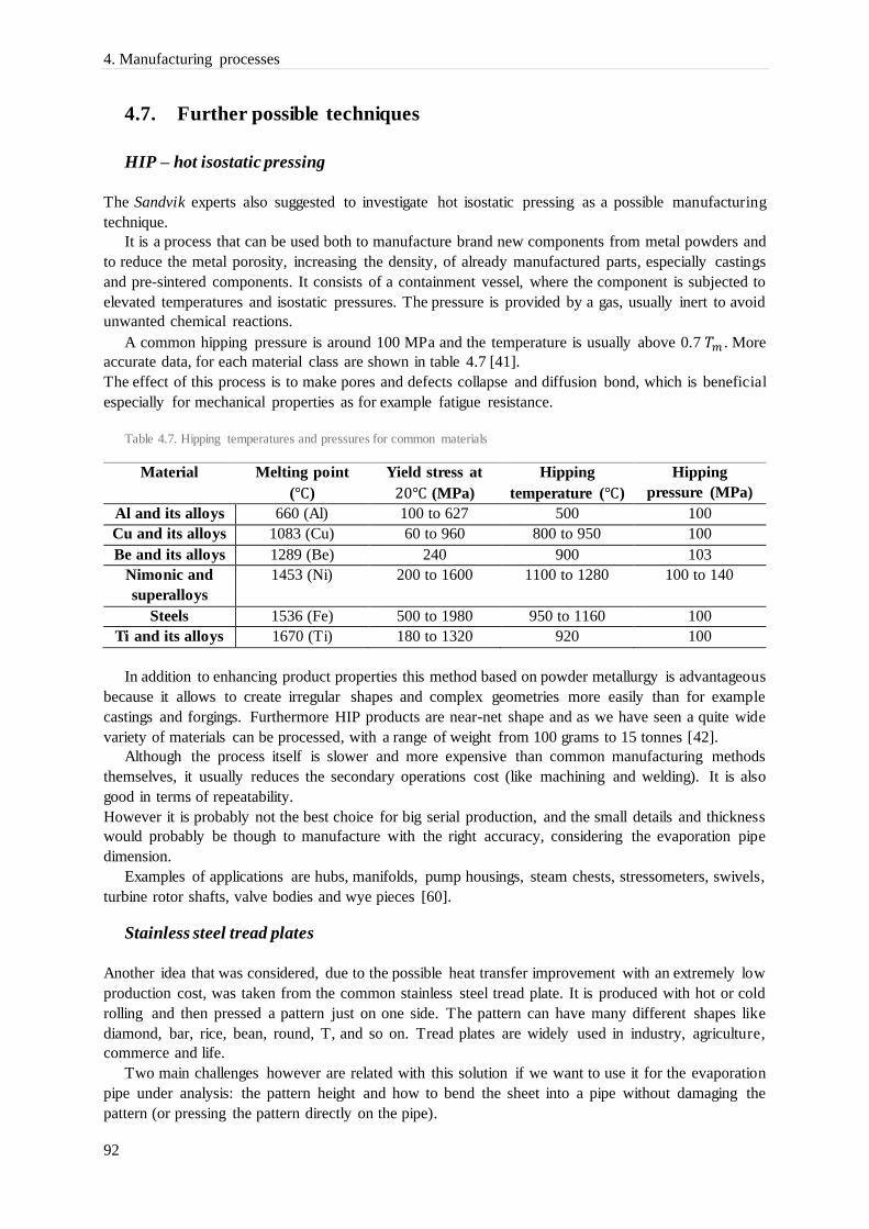
4. Manufacturing processes

92

4.7. Further possible techniques

HIP – hot isostatic pressing

The Sandvik experts also suggested to investigate hot isostatic pressing as a possible manufacturing

technique.

It is a process that can be used both to manufacture brand new components from metal powders and

to reduce the metal porosity, increasing the density, of already manufactured parts, especially castings

and pre-sintered components. It consists of a containment vessel, where the component is subjected to

elevated temperatures and isostatic pressures. The pressure is provided by a gas, usually inert to avoid

unwanted chemical reactions.

A common hipping pressure is around 100 MPa and the temperature is usually above 0.7 𝑇𝑚 . More

accurate data, for each material class are shown in table 4.7 [41].

The effect of this process is to make pores and defects collapse and diffusion bond, which is beneficial

especially for mechanical properties as for example fatigue resistance.

Table 4.7. Hipping temperatures and pressures for common materials

Material Melting point

(℃)

Yield stress at

20℃ (MPa)

Hipping

temperature (℃)

Hipping

pressure (MPa)

Al and its alloys 660 (Al) 100 to 627 500 100

Cu and its alloys 1083 (Cu) 60 to 960 800 to 950 100

Be and its alloys 1289 (Be) 240 900 103

Nimonic and

superalloys

1453 (Ni) 200 to 1600 1100 to 1280 100 to 140

Steels 1536 (Fe) 500 to 1980 950 to 1160 100

Ti and its alloys 1670 (Ti) 180 to 1320 920 100

In addition to enhancing product properties this method based on powder metallurgy is advantageous

because it allows to create irregular shapes and complex geometries more easily than for example

castings and forgings. Furthermore HIP products are near-net shape and as we have seen a quite wide

variety of materials can be processed, with a range of weight from 100 grams to 15 tonnes [42].

Although the process itself is slower and more expensive than common manufacturing methods

themselves, it usually reduces the secondary operations cost (like machining and welding). It is also

good in terms of repeatability.

However it is probably not the best choice for big serial production, and the small details and thickness

would probably be though to manufacture with the right accuracy, considering the evaporation pipe

dimension.

Examples of applications are hubs, manifolds, pump housings, steam chests, stressometers, swivels,

turbine rotor shafts, valve bodies and wye pieces [60].

Stainless steel tread plates

Another idea that was considered, due to the possible heat transfer improvement with an extremely low

production cost, was taken from the common stainless steel tread plate. It is produced with hot or cold

rolling and then pressed a pattern just on one side. The pattern can have many different shapes like

diamond, bar, rice, bean, round, T, and so on. Tread plates are widely used in industry, agriculture,

commerce and life.

Two main challenges however are related with this solution if we want to use it for the evaporation

pipe under analysis: the pattern height and how to bend the sheet into a pipe without damaging the

pattern (or pressing the pattern directly on the pipe).

4. Manufacturing processes

93

The pattern would be beneficial for the heat transfer both in terms of increased surface transfer and

turbulence generation which improves the convection on that surface. The best it would be thus to create

a pattern geometry that really makes a difference with respect to a simple sheet.

“Sandwich” solution

The sandwich solution, that is with a pipe of copper “coated” on both sides by a thinner stainless steel

pipe, has been thought to combine the best properties of both materials, that is high conductivity (copper)

and high corrosion resistance (stainless steel). This idea has been tested also for another project on a

different silencer and the results were promising. However it should be found a good way to join the

two different materials, and to make sure there won’t be any progressive phenomenon driven by the

quite high temperature going on at the boundary.

The first process that could be adopted is cladding, that is actually the one being used to manufacture

the copper pots stainless steel lined on the inner surface.

The bonding is achieved thanks to the high pressure applied between the surfaces of the different

materials layers, and therefore the possibilities are to extrude two metals together through a die or

pressing or rolling the sheets together (roll bonding).

Two other ways to achieve the same result is by explosive welding and laser cladding. In the first

one a chemical sheet of chemical explosive is used to press one layer against the other, avoiding heat

affected zones and expelling impurities. The second one instead is an additive manufacturing technology

where material is deposited on a surface and then melted and consolidated by the laser. Both of them

anyway are used a lot to increase corrosion resistance of metal sheets.

A good idea when applying this technique to the evaporation pipe for example, is to use materials

with similar expansion coefficients, because the component is subjected a lot to thermal cycles during

his life and the bonding can get damaged after a while. For this reason it is advisable to use an austenitic

stainless steel to coat the copper because despite having a lower conductivity than ferritic stainless steel,

it has the same thermal expansion coefficient as copper.

Another way to join the different layers is by using diffusion bonding, which a solid-state welding

process that allows contacting surfaces to be joined under pressure and elevated temperatures. Some

studies have been done about this topic, for example Yilmax and Aksoy [44] observed micro-voids and

micro-cracks into the material close to the interface, due to the Kirkendall effects, if direct bonding is

applied between Cu and stainless steel.

H. Sabetghadam et al [45] have joined AISI 410 stainless steel layer to a copper one using a nickel

interlayer at a temperature range of 800-950 ℃. The nickel minimizes the aforementioned problem. The

interdiffusion depth was highly influenced by the bonding temperature and it was around 20-30 𝜇𝑚.

Nevertheless due also to the high temperatures and long times to which the evaporation pipe is subjected

during its working diffusion could continue leading to a decrement in physical and mechanical properties

with time.

Moreover this process generally takes a considerable amount of time compared to other techniques,

and is quite expensive, resulting in a not optimal solution.

Super conductive foams

Super conductive foams were first introduced by a Japanese company called Lotus Thermal Solutions,

and they found good diffusion in heat sink applications for electrical components. They consist of a

porous metal (usually copper), with directional pores, obtained with a particular continuous casting

process where gas is added. The porosity and the pores diameter can be controlled pretty well with this

process, leading to a small, lightweight and high cost performant heat sink. The pores increase a lot the

surface available for convection giving really good heat transfer performances.

4. Manufacturing processes

94

Nevertheless they are specifically created for electronics application where the convection is forced

(some pumping work is needed) and the pressure drops are not important since, due to the small pores

dimension, they are pretty high. For example with a velocity of 0.2 m/s the pressure drop is around 2

kPa [43].

Their application in exhaust systems and especially in the evaporation module must then be rejected.

Techniques to attach the fins to the pipe

A common and usually quite cheap alternative is to attach the fins to the pipe in some way. It could be

realised in general with welding, epoxy-bonding, or press-fit bonding. In any of those cases anyway, the

pipe should first be manufactured and for pipes with a diameter of 0,152 m and less than 3 mm thick the

quickest and cheapest way to do it is by bending and welding a metal sheet.

Welded sheet pipe with fins welded on it

Considering the welding of the fins on the pipe, for sure a continuous welding method should be used.

This is basically because a good contact is needed between the fins and the pipe, to allow the heat to

flow through the fins to the pipe, without finding big contact resistances.

Considering then the dimension of the gaps between the fins, that should host the welding tool, the

available methods are basically narrowed down to two techniques: laser beam welding (LBW) and

electron beam welding (EBW). Other welding techniques as resistance welding or mag welding both

need a rather bulky tooling compared to the available space, and they would take a quite longer time.

LBW is the process used in the current manufacturing process, as it’s been mentioned earlier. It

employs a laser beam with high power density resulting in narrow deep welds and high welding rates.

The beam creates a very small heat affected zone and very high heating and cooling rates (in general

quite dangerous for cracking). The welding speed is proportional to the power supplied and to the

workpiece thickness, and since the laser (particularly the gas laser) has high power capabilities, the

process can be very quick compared to other welding techniques.

The laser welding is therefore a technique especially convenient for high volume production, mostly

paired with automated robots that helps improving its productivity.

LBW, in addition to guaranteeing high weld quality, represents a versatile process, being able to weld

several material as :

- Carbon steels

- HSLA steels

- Stainless steels

- Aluminium

- Titanium

The laser itself can be generated from two different media, solid state and gas. The first kind has

lower power outputs and is usually limited to pulsed mode, while the second one is suitable for

continuous welding and is able to reach a power output of 25 kW.

Moreover compared to electron beam welding, laser welding has some advantages:

- It doesn’t require vacuum as the EBW does

- It is easier to automate with robots

- No dangerous X-rays emission

- Higher quality welds

Considering then the 10000 unit/year production, the dimension of the gaps reserved to the welding,

the speed needed to cover all the 52 meters of welding necessary for the fins and the good welding

quality needed for the heat conduction, it is straightforward to see that laser welding is the most suitable

techniques for the evaporation pipe as it is.

4. Manufacturing processes

95

The other two methods mentioned above are instead used mostly in the electronics industry, but are

not good for the specific application studied in this thesis.

Press-fit bonding is done by using thicker fins than their slots where they are pressed, creating

interference. However it needs some slots already in the pipe, and since it is very thin, it is not advisable

to further reduce its thickness, even just locally. It also can be problematic with such thin and long fins

as the ones used currently (0,2 mm), besides requiring most likely more time than the laser welding.

Epoxy bonding instead is between the best high-performance adhesive techniques that can suit almost

any application and material, but its strength degrades above 177 ℃ making it unsuitable for exhaust

system components.

Hydroforming of the fins sheet

Hydroforming is a shaping technique which has large application in the automotive industry, since it

can produce lightweight, structurally stiff and strong components with complex shapes. Unibody

structures for sports cars or aluminium bicycle frames are very common products.

The process consists basically in forming the workpiece in a closed die at room temperature thanks

to the high pressure generated by the fluid injected by an hydraulic pump.

Two main kind of hydroforming can be performed: sheet hydroforming and tube hydroforming.

In both cases the process is limited by very high closing forces required to seal the die chamber where

the liquid is injected. However, theoretically very complex shapes can be produced in one step,

especially with thin metal sheets (like the folded one used for the fins welded on the evaporation pipe).

The tools are quite cheap and tight tolerances and high surface finish can be achieved.

The materials suitable for hydroforming are almost all the metals that can be cold formed like :

- Aluminium

- Brass

- Carbon and stainless steels

- Copper

- High strength alloys

It thus seems an interesting technique to substitute the stainless steel sheet folding, in case it

represents a time limiting and cost raising step for the current manufacturing process.

U ducts

The idea of manufacturing U ducts instead of a continuous folded sheet was basically to simplify the

current manufacturing process and reducing the time needed for the folding operation that would also

require probably a less complex sequence and fixturing.

The flow distribution, since the top connection between two fin walls is missing, would be affected,

but if we keep the same flanges height and number as the current design the differences shouldn’t be

much. Besides exactly the same tooling for the welding process can be used, without requiring further

investments.

Missing the cost breakdown for the process is hard to make an estimation on the cost saving that it

could generate, and compare it to the difference in performances, but it represents for sure a valid option.

4. Manufacturing processes

96

4.8. Summary

The manufacturing processes presented in this chapter have been evaluated in terms of :

- Cost

- Processing time

- Simplicity and Flexibility

- Geometrical limits

A summary of the main processes considered with their pros and cons is presented in table 4.8.

Table 4.8. Summary of the manufacturing processes characteristics

Process Advantages Disadvantages

Cold forming - Can be cheaper than the

current process

- Small details and thin walls

can be achieved

- Very good surface finish

and tolerances

- More than one step is required,

increasing the time needed

- Achievable fins shape is a

challenge

Extrusion - Quick process

- Rather cheap with “soft”

materials

- Cold extrusion has good

surface finish and

tolerances

- Difficult to achieve small details

as the fins, and thin walls (min.

3mm)

- Very difficult to extrude hard

materials like stainless steels

- Hot extrusion requires post-

process machining

Investment

Casting

- Complex geometries can be

achieved

- Good surface finish and

dimensional accuracy

- Repeatability

- Many different materials

can be cast

- Long production cycles

- High costs (difficult to reach a

lower price than the current

process)

- Minimum thickness of 3mm

- Maximum height of 3 times the

thickness

Machining - Few geometrical

constraints

- Extremely long time needed

- Highly expensive

- Difficult with hard materials

like stainless steels

HIP - Reduces secondary

operations cost

- Can obtain quite complex

shapes

- Slow

- Rather expensive

- Not the best for big serial

production

- Challenge for the accuracy

SS tread plates - Extremely cheap

- Quick

- Poor shapes achievable

- Probably not great evaporation

performances

Laser welding - Fast, and thus good for big

welding lengths

- Accurate

- Suitable for high volumes

production

- Easy to automate

- Not the best thermal contact

- Complex tools needed to keep

the component in position

- Rather expensive

Press fit bonding - Cheap - Problematic for the dimensions

4. Manufacturing processes

97

Epoxy-bonding - High performance adhesive

technique

- Poor behaviour at high

temperatures

“Sandwich”

solution

- Good thermal

performances

- Cladding is quite simple

- Rather long

- Some defects at the boundary

could occur

- Attention should be made to the

thermal expansion cycles

- Great thermal contact is needed

Superconductive

foams

- Compact and cheap

- Lightweight

- Very high pressure drops

introduced to enhance the heat

transfer

- Being usually made of copper

could require a protection

U ducts - Simpler and quicker

folding process

- Same tooling of the current

process can be used

- Require the quite long and

expensive laser welding

Fins sheet

hydroforming

(alternative to the

folding process)

- Cheap tools

- Tight tolerances and high

surface finish

- Complex shapes can be

produced in one step

- Quick

- The geometries needed can be

difficult to achieve, even with

more than one step

99

5. CFD simulations

This chapter is intended to evaluate with a DOE (design of experiments) some parameters influence on

the convection occurring on the finned surface. Those parameters are fins height, width and number.

Also some simple pipe designs are going to be included in the computation, but since the load needs to

be evenly distributed the tube’s thickness is not thought to play a big role.

In this way, however, it can be evaluated which fin geometry is the best one for the outer convection.

5.1. Equations governing CFD

The computational fluid dynamics analysis is a numerical method used to study fluid flows problems,

within fluid mechanics. It is based upon a famous group of equations called Navier-Stokes-Fourier, that

are basically balance equations of mass, momentum and energy.

Conservation of mass

𝜕𝜌

𝜕𝑡+ ∇ ∙ (𝜌 ∙ �̅�) = 𝜔

(5.1)

Which is a punctual equation consisting of three terms; the first one represents the mass variation in

time, the second one the mass variation due to mass flows from and to the analysed volume and 𝜔

represents a mass source/sink term.

Conservation of momentum

𝜕(𝜌 ∙ �̅�)

𝜕𝑡+ ∇ ∙ (𝜌 ∙ �̅� × �̅�) + ∇𝑝 = ∇ ∙ Π𝑣̿̿ ̿̿ + 𝜌 ∙ 𝑔

(5.2)

Where

Π𝑣̿̿ ̿̿ = 𝜌 ∙ 𝜐 (∇�̅� + ∇�̅�𝑇 −

2

3∇ ∙ �̅� ∙ 𝐼 ̿)

(5.3)

𝜕(𝜌∙�̅�)

𝜕𝑡 is a momentum variation in time,

𝜌 ∙ �̅� × �̅� is called advection flux,

𝑝 𝐼 ̿ is called static flux and

Π𝑣̿̿ ̿̿ is called dynamic flux, and represents the viscous contribution in the conservation of momentum

equation.

The last three terms can be also seen as stresses, having the same dimensions as a force per unit surface.

𝜌 ∙ 𝑔 is an example of momentum source/sink.

Conservation of total energy

𝜕(𝜌 ∙ 𝑒𝑡)

𝜕𝑡+ ∇ ∙ (𝜌 ∙ 𝑒𝑡 ∙ �̅� + 𝑝 ∙ �̅�) = ∇ ∙ (−𝑞 + Π𝑣̿̿ ̿̿ ∙ �̅�)

(5.4)

5. CFD simulations

100

Where

𝑞 = −Λ̿ ∙ ∇𝑇

(5.5)

constitutes the Fourier equation, already seen in chapter 2.

Again 𝜕(𝜌∙𝑒𝑡)

𝜕𝑡 is the total energy variation in time,

𝜌 ∙ 𝑒𝑡 ∙ �̅� the advective flux,

Π̿ ∙ �̅� = 𝑝 𝐼 ̿ ∙ �̅� − Π𝑣̿̿ ̿̿ ∙ �̅� the mechanical flux and

𝑞 the thermal flux.

In this case, being the total energy a conserved quantity, the source/sink terms are null.

5.2. Concept behind the simulations

The CFD simulations are highly needed to solve problems of high complexity, and thus to create a more

accurate model with respect for example to the one used in the second chapter. In this case all the local

convection coefficients, in each channel at different heights and depths, can be obtained and therefore

the results would be much closer to reality.

However they usually have need a balance between the discretization dimension and the time and

cost needed to solve those problems, despite the computational power of nowadays computers.

Indeed one of the biggest issues to simulate the evaporation pipe in the complete silencer model, is that

due to the dimensions of the fins, they have to be excluded, because the model would need a cell

dimension so small that the total computational time and cost would increase exponentially.

And it can be too long even when only the evaporation pipe is going to be analysed, if the fins are

included. The model, being 355 mm long and with a diameter of 152 mm, is big, compared to the

geometry of the fins, that needs to be resolved (width between 1 and 3 mm and height between 5 and 10

mm).

For that reason, since we want to run many different simulations in order to evaluate the influence of

some parameters, the model should be reduced in size in a smart way. That means that some

approximations should be done, but in a way that allows to have results the closest as possible to the

complete model and therefore to reality.

The idea is then to use a sector with only 3 fins, on which some parameters can be changed, in order

to obtain 50 different geometries. The simulations will then interesting results thanks to the periodic

boundary conditions that can be set on both sides. They would emulate the presence of a complete pipe,

repeating the sector as a pattern, but heavily reducing the computational time.

5.3. Parameters of DOE

The parameters that will be analysed are the ones that are thought to have a major influence on the heat

exchange on the flanges. Those are (fig. 5.1) :

- The fins height

- The fins width

- The fins number

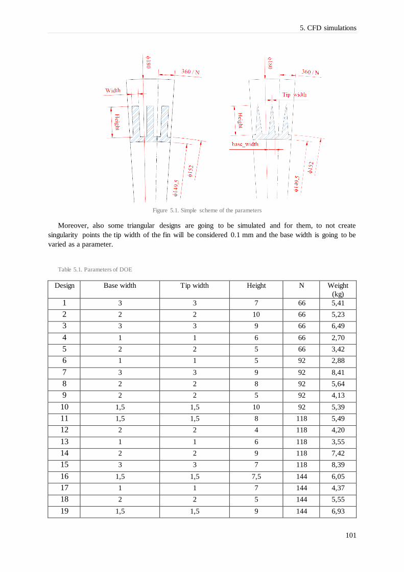
5. CFD simulations

101

Figure 5.1. Simple scheme of the parameters

Moreover, also some triangular designs are going to be simulated and for them, to not create

singularity points the tip width of the fin will be considered 0.1 mm and the base width is going to be

varied as a parameter.

Table 5.1. Parameters of DOE

Design Base width Tip width Height N Weight

(kg)

1 3 3 7 66 5,41

2 2 2 10 66 5,23

3 3 3 9 66 6,49

4 1 1 6 66 2,70

5 2 2 5 66 3,42

6 1 1 5 92 2,88

7 3 3 9 92 8,41

8 2 2 8 92 5,64

9 2 2 5 92 4,13

10 1,5 1,5 10 92 5,39

11 1,5 1,5 8 118 5,49

12 2 2 4 118 4,20

13 1 1 6 118 3,55

14 2 2 9 118 7,42

15 3 3 7 118 8,39

16 1,5 1,5 7,5 144 6,05

17 1 1 7 144 4,37

18 2 2 5 144 5,55

19 1,5 1,5 9 144 6,93

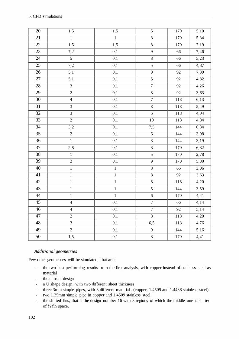
5. CFD simulations

102

20 1,5 1,5 5 170 5,10

21 1 1 8 170 5,34

22 1,5 1,5 8 170 7,19

23 7,2 0,1 9 66 7,46

24 5 0,1 8 66 5,23

25 7,2 0,1 5 66 4,87

26 5,1 0,1 9 92 7,39

27 5,1 0,1 5 92 4,82

28 3 0,1 7 92 4,26

29 2 0,1 8 92 3,63

30 4 0,1 7 118 6,13

31 3 0,1 8 118 5,49

32 3 0,1 5 118 4,04

33 2 0,1 10 118 4,84

34 3,2 0,1 7,5 144 6,34

35 2 0,1 6 144 3,98

36 1 0,1 8 144 3,19

37 2,8 0,1 8 170 6,82

38 1 0,1 5 170 2,78

39 2 0,1 9 170 5,80

40 1 1 8 66 3,06

41 1 1 8 92 3,63

42 1 1 8 118 4,20

43 1 1 5 144 3,59

44 1 1 6 170 4,41

45 4 0,1 7 66 4,14

46 4 0,1 7 92 5,14

47 2 0,1 8 118 4,20

48 3 0,1 6,5 118 4,76

49 2 0,1 9 144 5,16

50 1,5 0,1 8 170 4,41

Additional geometries

Few other geometries will be simulated, that are:

- the two best performing results from the first analysis, with copper instead of stainless steel as

material

- the current design

- a U shape design, with two different sheet thickness

- three 3mm simple pipes, with 3 different materials (copper, 1.4509 and 1.4436 stainless steel)

- two 1.25mm simple pipe in copper and 1.4509 stainless steel

- the shifted fins, that is the design number 16 with 3 regions of which the middle one is shifted

of ½ fin space.

5. CFD simulations

103

Table 5.2. Additional geometries parameters

Design Description Base width

(mm)

Tip width

(mm)

Height

(mm)

N Weight

(kg)

51 Nr10_Cu 1,5 1,5 10 92 6,26

52 Nr33_Cu 2 0,1 10 118 5,62

53 Current design 0,2 0,2 7,5 288 2,93

54 U duct 288 0,2 0,2 7,5 288 2,93

55 U duct 288

thick

0,4 0,4 7,5 288 4,24

56 3 mm Cu 0 0 0 0 4,56

57 3 mm FSS 0 0 0 0 3,93

58 3 mm ASS 0 0 0 0 4,08

59 1.25 mm Cu 0 0 0 0 1,88

60 1.25 mm SS 0 0 0 0 1,62

61 Shifted fins 0,2 0,2 7,5 288 2,93

62 U duct 136 0,2 0,2 11 136 2,5

5.4. Simplifications and boundary conditions

As already stated in par. 5.2, some simplifications are needed. First of all, as mentioned, just a sector of

the complete pipe is going to be simulated. Secondly, to reduce the dimension of the volume, just the

finned part of the pipe will be part of the model.

An “entrance” region, 50 mm long, has been added at the inlet, to be able to specify a global mass

flow, for both the inner and outer region of the pipe, and therefore in order to leave the flow distribute

itself between them, just based on the pressure drop that is going to encounter in the regions.

Also in the simulations the mixer presence, due also to the need of analysing just a sector of the pipe, is

going to be neglected.

Furthermore to emulate the urea presence and the consequent cooling effect caused on the pipe, a

heat sink will be employed. However it is going to be applied on the whole inner surface of the sector

analysed, resulting in a uniform distribution in the virtual complete pipe. This approximation will cause

a lower conduction influence on the minimum temperature reached in the pipe, and therefore the simple

pipe designs (the 3 mm ones) will have lower performances compared to the finned ones with respect

to reality and also the improvement introduced by an increase in thickness (from 1.25mm to 3mm) will

be reduced. The heat sink value, being a comparison problem and hence not making a big difference its

absolute value as long as it’s the same on each design, will be kept around 1000 𝑊/𝑚2 .

The boundary conditions that are going to be used are shown in fig. 5.2. On the inlet area the flow

temperature and the mass flow will be specified. They are respectively 300 ℃ and 800 𝑘𝑔/ℎ.

As already mentioned earlier a periodic boundary condition will be used both for the gas and solid sides.

This will lead to a periodical repetition of the solution, which is correct for symmetrical problems.

In addition the fins will represents the separation between the solid and the gas and the outlet will be

divided in an upper one (for the fins region) and a lower one (for the inner of the pipe), and in both of

them the atmospheric pressure is specified.

5. CFD simulations

104

In the end, the outer wall is considered adiabatic. This is basically because, being the silencer

insulated, the temperature in it will be high, sometimes higher, others lower, than the flow temperature

in the AdBlue evaporator depending also on the engine operation, therefore hardly predictable.

The physical properties used in the simulations are:

- Gas : air (see appendix A for its physical properties)

- FSS 1.4509 (𝑘 = 25𝑊

𝑚𝐾, 𝑐𝑝 = 460

𝐽

𝑘𝑔𝐾 , 𝜌 = 7700

𝑘𝑔

𝑚3)

- ASS 1.4404 (𝑘 = 15𝑊

𝑚𝐾, 𝑐𝑝 = 500

𝐽

𝑘𝑔𝐾 , 𝜌 = 8000

𝑘𝑔

𝑚3)

- Copper (𝑘 = 392𝑊

𝑚𝐾, 𝑐𝑝 = 384

𝐽

𝑘𝑔𝐾 , 𝜌 = 8940

𝑘𝑔

𝑚3)

Figure 5.2. Boundary conditions

5. CFD simulations

105

5.5. Results

The results of the CFD simulations are presented in fig. 5.3 in terms of minimum temperature in the

solid and pressure drop. The first quantity is the one chosen as indicator of the heat transfer performances

of each design, as already done in the previous FEM analysis and as it will be done in the tests.

Figure 5.3. Minimum temperature in the solid vs pressure drop

As expected the simple pipe designs, and especially the thinner and stainless steel made ones are the

worst. But surprisingly the current design is not the best performing one. The designs number 2, 10, 33

and 62 resulted having better performance, even if made with stainless steel, and this is due to the better

convection on the finned surface.

A good idea is then to plot the results also in terms of the parameters analysed, in order to see which

influence they do have on the performances.

As far as the fins number is concerned, it doesn’t seem to play a big role since the results are pretty

well distributed all over the graph. There is apparently a concentration of the best performances (lowest

temperature drop) between 66 and 118 fins, but this can be and it probably is related to another parameter

that will be analysed below.

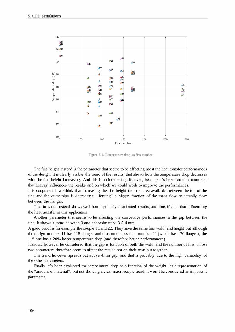
5. CFD simulations

106

Figure 5.4. Temperature drop vs fins number

The fins height instead is the parameter that seems to be affecting most the heat transfer performances

of the design. It is clearly visible the trend of the results, that shows how the temperature drop decreases

with the fins height increasing. And this is an interesting discover, because it’s been found a parameter

that heavily influences the results and on which we could work to improve the performances.

It is congruent if we think that increasing the fins height the free area available between the top of the

fins and the outer pipe is decreasing, “forcing” a bigger fraction of the mass flow to actually flow

between the flanges.

The fin width instead shows well homogenously distributed results, and thus it’s not that influencing

the heat transfer in this application.

Another parameter that seems to be affecting the convective performances is the gap between the

fins. It shows a trend between 0 and approximately 3.5-4 mm.

A good proof is for example the couple 11 and 22. They have the same fins width and height but although

the design number 11 has 118 flanges and thus much less than number 22 (which has 170 flanges), the

11th one has a 20% lower temperature drop (and therefore better performances).

It should however be considered that the gap is function of both the width and the number of fins. Those

two parameters therefore seem to affect the results not on their own but together.

The trend however spreads out above 4mm gap, and that is probably due to the high variability of

the other parameters.

Finally it’s been evaluated the temperature drop as a function of the weight, as a representation of

the “amount of material”, but not showing a clear macroscopic trend, it won’t be considered an important

parameter.

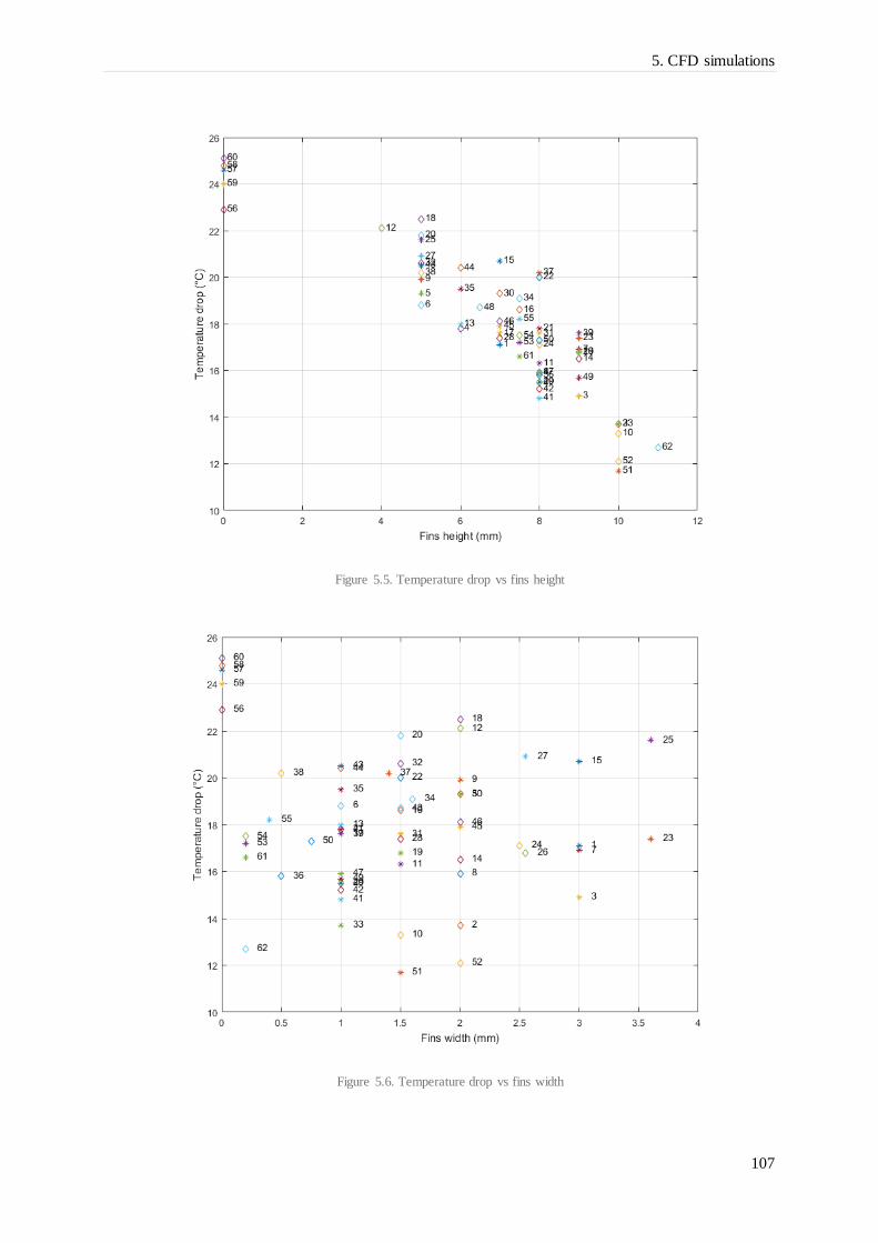
5. CFD simulations

107

Figure 5.5. Temperature drop vs fins height

Figure 5.6. Temperature drop vs fins width

5. CFD simulations

108

Figure 5.7. Temperature drop vs fins gap

Figure 5.8. Temperature drop vs pipe weight

5. CFD simulations

109

5.6. Summary and discussions

To summarize the CFD simulations that have been performed on the different fin designs showed that

an improvement in the heat transfer performances can be achieved by increasing the fins height. The

fins number can also be halved, giving a quicker and less expensive manufacturing process.

Nevertheless in this analysis, having applied a uniform load (representing the heat absorbed by

evaporating urea), the conduction influence is highly scaled down.

The results can be compared to the heat transfer study through correlations, where a critical height

seemed to be reached quite quickly for the current design and the number of teeth was rather important

to increase the heat transferred.

Although it was already clear that a lower number of fins could have been balanced by an increment

in fins height, the model couldn’t represent the actual importance of that height. Moreover the model

wasn’t able to depict the fins number actual influence, connected to the gap in between the fins. It is

straightforward to see that above a certain limit the number increment should become detrimental.

This deviations are most likely due to the consideration of the annulus as an overall volume (region in

between the fins plus region between the fins tip and the outer pipe wall), and therefore the convective

coefficient computed is an “overall” one. However most of the available surface is between the fins,

where the flow speed and therefore the convection is much lower.

111

6. Tests

The test goal is to evaluate the evaporation performances of each different fin design, and to see how it

can be correlated to the previous results. Different operating points will be tested for each design, by

changing both flow temperature and mass flow, as well as dosing rate.

6.1. Test rig

To do so, a test rig previously developed for a similar purpose is available and that represents a great

advantage but at the same time a constraint.

Indeed it allows to save much time and efforts in its design and manufacturing, nevertheless the test

itself and the test specimen have to be conceived in order to fit the test rig. In figure 6.1 the available

test rig is presented.

Figure 6.1. Previously available test rig

The gross dimensions of the rig are shown in table 6.1.

Table 6.1. Gross dimensions of the test rig

Length (mm) 942

Width (mm) 201

Height, with handles (mm) 326

The first constraint is the dimensions of the inner volume that can’t accommodate a complete

evaporation pipe but just a “small” section of it.

6. Tests

112

Secondly as it could be seen from fig.1 there are just six holes (marked in red) that can be used to fix

the test specimen onto the rig. Since more than one specimen is going to be tested and due to the need

of flexibility (for the difference there could be between different specimens) screws will thus be the only

option to do it.

Furthermore the bottom surface has many obstacles that can create obstructions in the flow and local

turbulence that are probably going to cause further deviations from the reality. In order to prevent this

then a plate is going to be designed, to be used as a flat floor that will play the role of the outer pipe’s

inner surface. the plate needs to be as conform as possible to the housing to avoid air to go below it.

Figure 6.2. Updated test rig section

Four windows are clearly visible from fig. 6.1 and they need both for the visual inspection and for

possible IR camera filming to record the temperatures on the upper surface of the specimen.

To avoid air and urea vapours leakages both the two ends and all the windows and lids, need to be well

tightened, and the use of a sealing silicon will be necessary.

6.2. Specimen

The specimen to not influence urea film creation, and potential deposit formation, as well as to emulate

in the best way the actual pipe, needs to have a smooth upper surface. It will then for this reason be

adopted a solution that includes the welding of six screws (by the head) on the lower surface of the test

specimen. In this way they can then be fastened with a simple nut from below the rig.

It has therefore been chosen a plate to emulate the pipe portion for the mentioned reasons as well as for:

- Simplicity of screw welding on it

- Conformity with the floor

- Easier fitting

The plate will then be positioned with the smooth part in direction of the AdBlue dosing unit, and

with the finned part, were the screws are welded, below. The distance between the test plate and the

“floor” needs to be such that it creates a similar mass flow distribution and thus velocities on the two

surfaces but also that it prevents all the lower flow to leave the finned region in favour of the free place

between the fin tip and the floor.

6. Tests

113

Figure 6.3. Test plate

Some spacing sleeves will be used to set the wanted distance between the plate and the floor. Their

dimensions are :

Table 6.2. Spacing sleeve dimensions

Figure 6.4. Spacing sleeve dimensions

As a consequence of all these constraints, the screws chosen are M8 x 45.

The screw welding will be a delicate operation since it requires good accuracy in screw positioning to

make sure that every screw body is fitting the holes in the rig.

6.3. Temperature sensors and positioning

Figure 6.5. Test plate with sensors positioning

To measure the plates temperatures 7 thermocouples will be mounted on the lower side, the finned one,

in strategic positions and in order to be able to get some interesting temperature behaviours.

For thread d D L

M8 9 18 10

M8 8.5 16 12

M8 8.5 15 16

6. Tests

114

Figure 6.6. Test plate with sensors

The sensor number 7 is the first encountered by the flow, and will then be in every different test the

one with the highest temperature, since it won’t ever be hit by the spray. The dosing unit is indeed angled

of 10 degrees and thank also to the flow the wet area will be almost in the centre of the plate. Sensor 6

instead is in a position that depending on the flow rate and temperature can be wet or not. The other

sensors, with some exceptions for number 1, are generally covered by the urea film.

Those temperature sensors are thermocouples type K, from Pentronic, that is one of Europe’s largest

manufacturers of industrial temperature sensors.

The thermocouple functioning principle was discovered by Seebeck in 1821. It consists of a pair of wires

connected together at one end to create a measuring junction. The junction, made by soldering, has to

be electrically conductive in order to be able to generate an electromotive force in the circuit, closed at

the other end where the measuring instrument is connected.

Figure 6.7. Thermocouple sensor used (the measuring junction is separated to show the two wires)

On every metal wire placed in a temperature gradient, a Seebeck voltage will occur over the entire length

of the gradient. The steeper the gradient, the higher the voltage at that point.

The output voltage on each wire can be written as

𝐸𝑖 = 𝑆𝑖 ∙ (𝑇1 − 𝑇2) (6.1)

6. Tests

115

where S is the Seebeck coefficient, constant for each material. In a thermocouple each wire has a

different Seebeck coefficient.

For the complete thermocouple it is then given

𝐸𝐴𝐵 = 𝐸𝐴 − 𝐸𝐵 = (𝑆𝐴 − 𝑆𝐵)(𝑇1 − 𝑇2) (6.2)

which can be re-written as

𝐸𝐴𝐵 = 𝑆𝐴𝐵(𝑇1 − 𝑇2) (6.3)

This voltage can then be measured, and as it can be easily deducted from eq. 6.3 it varies with the

temperature difference over the wires.

Figure 6.8. Circuit of a type K thermocouple

The type K sensor [1] has a temperature range of -200 – 1300 °C and is good in oxidizing

environments but not suitable for reductive environments such as sulphur, cyanide, carbon and hydrogen.

The one that is going to be used has also a glass fiber coating able to resist to high temperatures.

The materials of the two wires forming the thermocouple type K are Chromel (Ni-Cr) and Alumel (Ni-

Al).

Thermocouples need to be calibrated before being used, but in case it won’t be done, the measuring

uncertainty would be equal to the standard manufacturing tolerances characterizing the sensor.

For the type K sensor, the tolerances listed in table 3 apply.

Table 6.3. Pentronic type K tolerances specifications [46]

Tolerance class 1

(°C)

Tolerance class 2

(°C)

Tolerance class 3

(°C)

Temperature range −40 < 𝑇 < 1000 −40 < 𝑇 < 1000 −200 < 𝑇 < 40

Greatest of :

±1.5

or

±0.004 ∙ |𝑇|

±2.5

or

±0.0075 ∙ |𝑇|

±2.5

or

±0.0075 ∙ |𝑇|

6.4. Design of experiments

The test will be performed on 6 different operating points for each design, in order to evaluate a possible

difference in relative performances at different combinations of temperature and mass flow. The best

design should ideally achieve the best results in every condition.

In table 6.6 are showed the operating points chosen, between all the experiments’ combinations. Each

tested point is marked with the AdBlue dosage decided to be the best suited for it. It must anyway be

considered that for the dosing unit utilized the minimum amount of AdBlue that could be injected each

minute, without creating possible issues and uncertainty factors on the dosage, it is 5 𝑔/𝑚𝑖𝑛.

6. Tests

116

Table 6.4. All test combinations chosen for each plate

200 ℃ 250 ℃ 300 ℃ 350 ℃

400 𝑘𝑔/ℎ - - 5 𝑔/𝑚𝑖𝑛 -

450 𝑘𝑔/ℎ 5 𝑔/𝑚𝑖𝑛 - - -

700 𝑘𝑔/ℎ 5 𝑔/𝑚𝑖𝑛 5 𝑔/𝑚𝑖𝑛 - -

800 𝑘𝑔/ℎ - - 10 𝑔/𝑚𝑖𝑛 -

1000 𝑘𝑔/ℎ 5 𝑔/𝑚𝑖𝑛 - - -

6.5. Test cell system

The test cell used for the tests is called AR1, and is a cell used for exhaust after-treatment studies. The

complete cell is controlled by a software developed within Scania and named Scania Testbed Platform

(STP), which the user can command either by manually inserting values or by programming automated

test sequences.

The system is made by an electric fan, able to provide air flow rates from 0 to 2500 kg/h. The flow is

directed with several valves through an heater which turns on with a required flow temperature over 120

℃ and is capable of heating up the flow up to 550 ℃. Once the heater is turned on it reaches in few time

700 ℃ and stays at that constant level, regulating the flow temperature thanks to the valves that mix the

hot air, with some fresh air from outside.

Figure 6.9. Test rig system during an automated test

6. Tests

117

Figure 6.10. Heating system

Figure 6.11. AR1 test cell control station

6. Tests

118

Figure 6.12. Test rig with components

6.6. The dosing unit

The dosing unit that will be used has a fixed amount of AdBlue sprayed for each opening, and to vary

the AdBlue mass flow, it is just varying the frequency of the nozzle openings. This is an easy and

effective way to control the amount of AdBlue injected.

It could anyway create some problems if the upper and lower limits are going to be crossed. For example,

when the amount of AdBlue required is too high the frequency would be such that the nozzle is always

open and then it would be impossible to increase the dosage even more. This is basically because the

nozzle has a fixed amount of time needed to open and close, and thus the opening frequency can’t be

higher than a certain value.

This is not anyway the case of this study, since the plate is just a portion of the pipe, and the test-rig

is also subject of great heat losses to the environment, and therefore the amount of urea that is going to

be sprayed is really low (with respect to the normal dosage).

Figure 6.13. Dosing unit used for the tests

6. Tests

119

6.7. Test procedure

It is straightforward to understand that the plate at a certain temperature, if it is going to be cooled down

by a constant amount of AdBlue sprayed on it each minute (basically an AdBlue mass flow) an

equilibrium condition would be reached. This is when the heat absorbed by the AdBlue is equal to the

heat transferred to the plate by the gas flow.

On the temperature it is therefore going to be observed a transient condition, as soon as we start

dosing on the plate, which is then turning into a steady state condition in a certain amount of time.

This time span will be called 𝜏𝑖 , and being different for each design, will be evaluated to have a measure

of the specimen thermal inertia.

In general the transient duration can be different for each sensor, having in each part of the plate

potentially a different condition in terms of film presence and thickness, resulting in a different

temperature behaviour. Anyway if we look at them they won’t be substantially different. An average

value of them characterising the complete plate, can then be evaluated to see how fast each design “reacts”

and to compare them.

The idea is then to heat up the plate with the flow set to the temperature and mass flow it is going to

be tested. By trying with many time spans, 20 minutes it’s been verified being enough to reach the

correct condition before starting dosing, for any plate.

The dosing will then be enabled and will be kept at the same level again for 20 minutes, in order to let

the temperatures reach the new steady state condition. At the end of this time span, the dosing will be

stopped and the plate will be able to reach again the condition prior to the dosing.

Since you could find a lot of liquid on the plate that, especially at the rear edge of the plate, could

lead into deposits, a “cleaning” cycle will then be executed, at high temperature and high mass flow, to

blow away everything from the upper surface of the specimen.

Successively a new operating point can be set, exactly as done with the previous one, and thus starting

a new complete cycle. In this way the procedure can be automated, and many different combinations of

flow temperature and mass flow can be tested during the same session.

Figure 6.14. Example of a test performed on a FSS 1.25 mm thick simple plate

Controlled parameters (fig. 6.15):

𝑇𝑓𝑙𝑜𝑤 : flow temperature, measured by a sensor positioned upstream the test rig

6. Tests

120

�̇�𝑓𝑙𝑜𝑤 : mass flow

�̇�𝐴𝑑𝐵𝑙𝑢𝑒 : AdBlue dosing quantity

Other measured parameters

𝑝𝑖𝑛 : pressure at the test rig inlet

𝑝𝑜𝑢𝑡 : pressure at the test rig outlet

From fig. 6.14 we can see that the plate at the steady state, before starting dosing, is not at the same

temperature as the flow (i.e. what it was expected). But it could be easily explained by considering the

presence of the screws and all the heat losses from the test rig.

Furthermore the sensor number 7 is always the one with the highest temperature, and this agrees with

the expectations, being the first point in contact with the flow, that won’t be hit by the AdBlue.

It is interesting to observe the behaviour of sensors 4 and 6. They are respectively the one in the

middle of the plate, and the one before it in the flow direction. With a low temperature and a low mass

flow, the film is existing on a bigger area, and the spray is hitting the plate a bit more upstream, resulting

in a lower temperature reached on sensor 6. As soon as the temperature and/or the mass flow are

increased, leading to a different spray impact and wet area position, sensor number 4 is becoming the

lowest in temperature.

Figure 6.15. AdBlue dosing, flow temperature and mass flow during the test

Using just a plate, with a limited width and length, and being also difficult to control its horizontality

through the screws tightening, some liquid falling from the plate both on the sides and the end of the

plate can be observed. An idea to prevent the side flow is the use of a round sector instead of the plate,

but this anyway would probably mean a bigger flow down the final edge.

Nevertheless by looking at the results it seems to not influence heavily the steady state condition reached

after few time dosing, that is what we are interested in.

In fig. 6.14 and 6.14 is showed an example with just 2 combinations of flow temperature and mass

flow, but actually for each design, a long cycle script has been developed to be able to automatically run

the cell for long times, even overnight sometimes. An example of it is presented in fig 6.16 and 6.17.

6. Tests

121

Figure 6.16. Example of a long test cycle

Figure 6.17. Parameters of the long test cycle

6.8. Performance evaluation

As already done in the former chapters, the performances will be assessed by looking at the minimum

temperature reached on the plate, that is the most dangerous one. The worst design will be the one with

the lowest temperature.

The temperature measurements are going to be done with the temperature sensors on the lower side

of the plate. They won’t be the lowest temperatures between all, but the temperature gradient through

the plate is considered to be very low with respect to the temperatures reached, and the temperatures

won’t thus be substantially different on the upper side.

6. Tests

122

Due to unavailability of radiation transparent glasses it won’t be possible to use the IR camera to record

the upper temperatures, and the film temperature, and to verify the previous assumption.

The coefficient of performance will then be based on the temperatures measured at the steady state,

while dosing, and it will be defined by a ratio. This is a way to refer every result to the results achieved

with the current design, and hence to obtain relative values instead of absolute values, and base the

comparison on those. This coefficient, with a meaning similar to an efficiency, could be defined by two

different ratios.

The simplest one, is just by comparing the lowest temperature and thus:

𝐶𝑖 =

𝑇 𝑚𝑖𝑛𝑖𝑇 𝑚𝑖𝑛𝑐𝑢𝑟𝑟

(6.4)

while the other possibility is to compare the temperature drops with respect to the flow temperature of

different designs :

𝐶𝑖 =

𝑇𝑓𝑙𝑜𝑤 −𝑇𝑚𝑖𝑛𝑐𝑢𝑟𝑟

𝑇𝑓𝑙𝑜𝑤 − 𝑇𝑚𝑖𝑛𝑖

(6.5)

Being the temperatures absolute values pretty high, the second definition resulted the best one. It

gives a bigger difference between the designs, allowing to analyse more easily the results. (fig. 6.18 and

6.19). Furthermore it is also coherent with the one used in the FEM analysis.

6.9. Results

The tested plates/ designs are:

- 1.25 𝑚𝑚 ferritic stainless steel plate (1.4509), without fins

- 3 𝑚𝑚 ferritic stainless steel plate (1.4509), without fins

- Current design in ferritic stainless steel (1.4509)

- 1.25 𝑚𝑚 copper plate, without fins

- 3 𝑚𝑚 copper plate, without fins

- 3 𝑚𝑚 austenitic stainless steel plate (1.4404), without fins

- Design #12 in ferritic stainless steel (1.4509)

6. Tests

123

Figure 6.18. Performance coefficient in terms of minimum temperatures

Figure 6.19. Performance coefficient in terms of temperature drops

6. Tests

124

It is noteworthy to point out how both the simple copper plates, as well as in some cases also the

simple 3mm stainless steel plate, perform better than the current design, especially at low mass flow and

temperature. But also the finned design #12, although the 800 kg/h, 300 ℃ seems to be out of scale,

results to have the same or even lower temperature drops compared to the current design.

Furthermore if we consider the time needed to reach the steady state condition we can get an idea of

the thermal inertia of each design. The transient time has been evaluated by considering the time needed

for each sensor to reach 93% of its temperature drop at 450 kg/h, 200 ℃, as soon as the dosing starts.

The transient times obtained in this way are then summarized in their average value, which becomes a

constant typical of the plate. The lower this value, the lower is the time needed to heat up the potential

pipe at the start, but also lower would be the time needed to cool down the pipe when AdBlue is sprayed.

Figure 6.20. Transients time needed to reach the steady state condition after starting dosing at 450 𝑘𝑔/ℎ and 200 ℃

As expected, the 3 mm plate made of austenitic stainless steel (1.4404), having more material and at

the same time the lowest thermal conductivity, is the one with the highest transient time. However it is

just 18 % longer than the current design, and 4% longer than the 3 mm ferritic (1.4509) one.

Looking at the mass in table 6.7 and assuming that with the same thermal conductivity the transient time

should be proportional to the convection and the mass of the specimen, it is clear that the convection on

the finned surface of the current design is not really effective. The design #12 in fact, although having

a quite bigger mass has a lower transient time.

Table 6.5. Mass and transient times of the tested prototypes

Design Volume (m^3) Mass (kg) Transient time (s)

1.25mm FSS 5,95E-05 0,46 81,01

3mm FSS 1,43E-04 1,10 142,81

Current design 1,12E-04 0,86 125,67

1.25mm Cu 5,95E-05 0,53 56,14

3mm Cu 1,43E-04 1,28 59,86

3mm ASS 1,43E-04 1,14 148,33

Design #12 FSS 1,46E-04 1,13 120,00

6. Tests

125

In general conduction appears to be by far the heavier factor, while the convection on the finned surfaces

is not playing an important role.

This can see a verification in what we registered in both tests with the finned designs. One of them is

depicted in fig 6.21.

Figure 6.21. Deposits witnessing urea flow backwards between the fins

As it can be clearly seen, some urea was flowing in the opposite direction of the flow in between the

fins. The effect can be explained by a sort of capillary action, but it would for sure be avoided if we had

some actual flow between the fins. This means that the air is almost not flowing in the fin gaps, nullifying

the convection effect on the additional surface introduced by the fins. It is therefore clarified the better

performances of both the copper plates.

One reason for that could be that the plate is too far from the floor, leaving too much area between

the fins tip and the bottom plate for the air to flow. The pressure drop through the fins would then cause

almost all the flow to go in that free region. Nevertheless, also the free region above the plate is too big

to effectively emulate the pipe in pipe configuration. If the plate is moved downwards, a smaller air

quantity would flow below the plate, giving likely the same issues as earlier.

A possible solution can be the adoption of a device able to create a pressure drop in the area above

the plate (forcing some air to flow below), but without affecting too much the convection on the upper

surface.

On the other hand the tests resulted in being able to compare different materials and thicknesses of

the simple plates, resolving rather well the differences introduced by a change in one of the two factors.

The 3 mm simple plate made of austenitic stainless steel is having nearly the same temperature drops as

the one made by ferritic stainless steel, having a slightly lower thermal conductivity but also a slightly

bigger specific heat value. The other variabilities typical of every test execution make them reach the

same results.

127

7. Conclusions

The heat transfer analysis through correlations gave us results quite divergent from the following CFD

simulations. A refinement that can be done is to consider the annulus region as two separated regions,

one between the fin tip and the outer wall and one between the flanges, continuously exchanging mass

and energy. Nevertheless the FEM analysis performed allowed to understand the continuous balance

between convection and conduction which is affecting the temperature drop on the pipe. Depending on

the mass flow and on the temperature, one would be more influent than the other.

The finned surface resulted being more effective at lower mass flows and with a smaller film area,

while at higher mass flows thermal conductivity and thickness become gradually more influent with that

kind of unevenly distributed loading.

As far as the material is concerned, ferritic stainless steel (1.4509) proved to be an accurate choice,

a good trade-off between cost and both thermal and corrosion performances. The only alternative that

would make quite a big difference in thermal performances, without increasing too much the component

cost, nowadays is the CuCrZr alloy (almost pure copper). However it brings with it some possible issues

both with the maximum temperatures reached (and thermal cycles that the pipe undergoes) and with

corrosion in that environment. It would for sure require a protection coating and some analysis of the

stresses introduced by different thermal expansions due to the different materials.

Looking at the manufacturing processes, many alternatives to the current process have been depicted.

Extrusion and investment casting must be rejected due to the minimum thickness required. Investment

casting was also more expensive than the current process. Machining, especially with stainless steel, is

far too expensive and time consuming. A good alternative to the current process, that could achieve solid

fins at a lower cost is a multi-step cold forming process.

Furthermore some improvements can be introduced in the current process, in order to simplify it and

reduce both cost and processing time. The fins sheet folding can be executed with an hydroforming

process, or it can be divided in a simpler operation, that is folding each channel in a U shape on its own.

This last option involves a slightly different design but as we have seen this wouldn’t create a substantial

difference with the current one.

With the CFD simulations convection has been deeper analysed. The sensitivity of the heat transfer

performances to the fins geometrical parameters and thus their shape variation has been investigated.

The parameter that most clearly and directly appears affecting the temperature drop on the pipe is the

fins height. An increase of 46 % in height (3.5 mm on a height of 7.5 mm) can improve the performances

by almost 40% (with half the fins), at 800 kg/h and 300 ℃. Better heat transfer performances (lower

temperature drop) would mean better evaporation performances and lower risk of urea deposits, because

their formation thresholds would be shifted at higher AdBlue dosages.

Moreover, the gap between the fins below a threshold (around 3 mm) is penalizing the convection,

meaning that the fins number can be reduced, without actually disadvantaging the performances. This

reduction has also the consequence of requiring a smaller distance of laser welding and less angular

shifts of the assembly in the welding operation, resulting in time and hence cost drop.

In the end, in general the tests performed showed a poor ability to evaluate the heat transfer

performances increment introduced by the fins, since the flow in the finned region is very low, almost

nullifying the effect of the enhanced surface. Although good results have been achieved in comparing

different materials, the test rig itself is not the best suited for the fins design analysis and it can’t represent

a final validation of them. It is then advisable to focus and invest resources at early stages in simulating

7. Conclusions

128

through CFD the convection on each design, and then map the accurate convection coefficients obtained

on a FEM model, where an uneven distribution of the thermal load can be studied. It is however a rather

complex study case because the convection coefficients themselves depend on the load distribution.

After that the only reliable testing that can be performed is on the complete pipe in pipe configuration

used in the silencer.

The finals suggestion, if a cost reduction and performances improvements are pursued, considering

that no further investments are required in the process tooling, is to increase the height of the current

fins, and halve them. The welding operation would require basically half of the time employed now, and

if the previous folding operation represents then a bottleneck it can be accelerated with the mentioned

techniques (e.g. using U shaped fins). Furthermore since the fins number reduction involves a weight

drop, it becomes possible and beneficial a thickness increment, from 1.25 mm to 2 mm. The final weight

would be 3,94 kg compared to 3,34 kg which is the weight of the currently used finned pipe (just 18%

bigger). Two models of two recommended designs are shown in appendix E.

7.1. Recommendations for future work

As already mentioned in the future the first theoretical model used can be improved, by considering the

annulus region as two separated volumes, one between the fin tip and the outer wall and one between

the flanges, continuously exchanging mass and energy.

It would also be interesting to run more CFD simulations, varying the number of fins and keeping a

constant fins height, to be able to distinguish better the effects of each parameter. At the same time it is

worthy to test a bigger heat sink on the inner wall, to see if the results are scalable.

For future studies of this system, I would recommend to focus more on CFD simulations and their

interface with FEM analysis, in order to be able to predict well what is happening in reality, without

requiring an intermediate testing of which we are not 100% sure about its reliability. Surely some tests

on the full scale pipe in pipe configuration would be necessary after that.

Another investigation that can be of interest is an analysis of how the walls surface (where the urea

film is occurring) roughness and irregularities are affecting the deposit formation, since different

manufacturing processes usually mean different roughness, in case a post-machining is not performed.

For example by only using different welding processes different results can be seen on the inner surface.

Finally, it can be said that finding a simplified testing method to have reliable results is pretty hard,

since the phenomena happening in the pipe in pipe, also with the mixer and the other components can

be quite unique. Moreover, during normal operations, the transient behaviour of the pipe is also rather

important.

129

Appendix A : Air Properties

Table 8. Physical properties of air at p=101.13 kPa

𝑻 (𝑲) 𝝆 (

𝒌𝒈

𝒎𝟑) 𝒉 (

𝒌𝑱

𝒌𝒈) 𝒔 (

𝒌𝑱

𝒌𝒈 𝑲) 𝑪𝒑 (

𝒌𝑱

𝒌𝒈 𝑲)

𝝁 (𝟏𝟎−𝟒 𝑷𝒂) 𝒌(

𝑾

𝒎 𝑲)

260 1.340 260.0 6.727 1.006 0.165 0.0231

280 1.245 280.2 6.802 1.006 0.175 0.0247

300 1.161 300.3 6.871 1.007 0.185 0.0263

350 0.995 350.7 7.026 1.009 0.208 0.0301

400 0.871 401.2 7.161 1.014 0.230 0.0336

450 0.774 452.1 7.282 1.021 0.251 0.0371

500 0.696 503.4 7.389 1.030 0.270 0.0404

600 0.580 607.5 7.579 1.051 0.306 0.0466

800 0.435 822.5 7.888 1.099 0.370 0.0577

1000 0.348 1046.8 8.138 1.141 0.424 0.0681

1200 0.290 1278 8.349 1.175 0.473 0.0783

1400 0.249 1515 8.531 1.207 0.527 0.0927

130

Appendix B : Reynolds and friction factor for the

different designs

Solid rectangular longitudinal fins

Figure 8.1. Reynolds number in the annulus, for SRL fins

Figure 8.2. Reynolds number in the inner pipe, for SRL fins

Appendix B : Reynolds and friction factor for the different designs

131

Figure 8.3. Friction factor in the annulus, for SRL fins

Solid triangular longitudinal fins

Figure 8.4. Reynolds number in the annulus, for STL fins

Appendix B : Reynolds and friction factor for the different designs

132

Figure 8.5. Reynolds number in the inner pipe, for STL fins

Figure 8.6. Friction factor in the annulus, for SRL fins

Appendix B : Reynolds and friction factor for the different designs

133

Longitudinal fins with the current design

Figure 8.7. Reynolds number in the annulus, for current fins

Figure 8.8. Reynolds number in the inner pipe, for current fins

Appendix B : Reynolds and friction factor for the different designs

134

Figure 8.9. Friction factor in the annulus, for current fins

Longitudinal fins with the U shape design

Figure 8.10. Reynolds number in the annulus, for U shape fins

Appendix B : Reynolds and friction factor for the different designs

135

Figure 8.11. Reynolds number in the inner pipe, for U shape fins

Figure 8.12. Friction factor in the annulus, for U shape fins

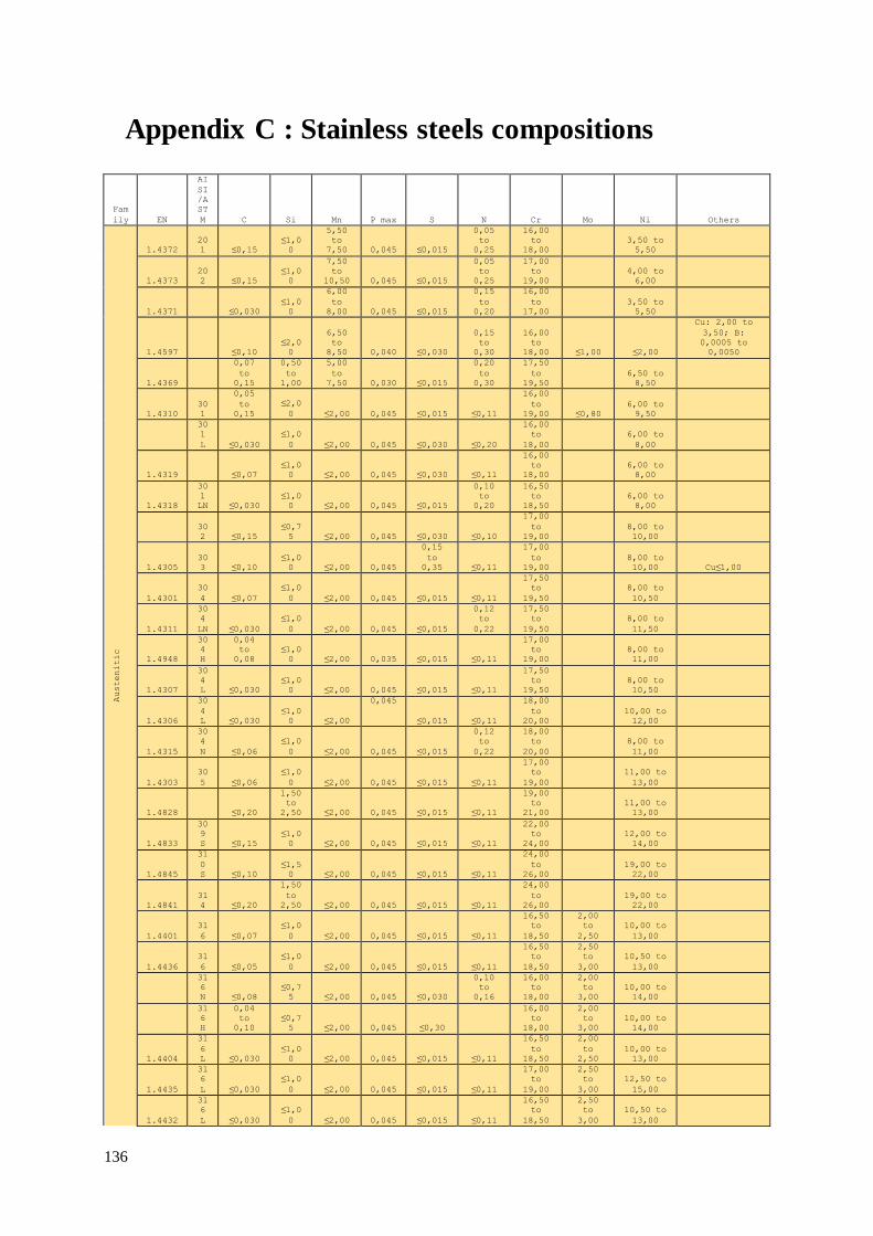
136

Appendix C : Stainless steels compositions

Fam

ily EN

AI

SI

/A

ST

M C Si Mn P max S N Cr Mo Ni Others

Austenitic

1.4372

20

1 ≤0,15 ≤1,00

5,50

to

7,50 0,045 ≤0,015

0,05

to

0,25

16,00

to

18,00

3,50 to

5,50

1.4373

20

2 ≤0,15 ≤1,00

7,50

to

10,50 0,045 ≤0,015

0,05

to

0,25

17,00

to

19,00

4,00 to

6,00

1.4371 ≤0,030 ≤1,00

6,00

to

8,00 0,045 ≤0,015

0,15

to

0,20

16,00

to

17,00

3,50 to

5,50

1.4597 ≤0,10 ≤2,00

6,50

to

8,50 0,040 ≤0,030

0,15

to

0,30

16,00

to

18,00 ≤1,00 ≤2,00

Cu: 2,00 to

3,50; B:

0,0005 to

0,0050

1.4369

0,07

to

0,15

0,50

to

1,00

5,00

to

7,50 0,030 ≤0,015

0,20

to

0,30

17,50

to

19,50

6,50 to

8,50

1.4310

30

1

0,05

to

0,15

≤2,0

0 ≤2,00 0,045 ≤0,015 ≤0,11

16,00

to

19,00 ≤0,80 6,00 to

9,50

30

1

L ≤0,030

≤1,0

0 ≤2,00 0,045 ≤0,030 ≤0,20

16,00

to

18,00

6,00 to

8,00

1.4319 ≤0,07 ≤1,00 ≤2,00 0,045 ≤0,030 ≤0,11

16,00

to

18,00

6,00 to

8,00

1.4318

30

1

LN ≤0,030 ≤1,00 ≤2,00 0,045 ≤0,015

0,10

to

0,20

16,50

to

18,50

6,00 to

8,00

30

2 ≤0,15 ≤0,75 ≤2,00 0,045 ≤0,030 ≤0,10

17,00

to

19,00

8,00 to

10,00

1.4305

30

3 ≤0,10 ≤1,00 ≤2,00 0,045

0,15

to

0,35 ≤0,11

17,00

to

19,00

8,00 to

10,00 Cu≤1,00

1.4301

30

4 ≤0,07

≤1,0

0 ≤2,00 0,045 ≤0,015 ≤0,11

17,50

to

19,50

8,00 to

10,50

1.4311

30

4

LN ≤0,030

≤1,0

0 ≤2,00 0,045 ≤0,015

0,12

to

0,22

17,50

to

19,50

8,00 to

11,50

1.4948

30

4

H

0,04

to

0,08

≤1,00 ≤2,00 0,035 ≤0,015 ≤0,11

17,00

to

19,00

8,00 to

11,00

1.4307

30

4

L ≤0,030 ≤1,00 ≤2,00 0,045 ≤0,015 ≤0,11

17,50

to

19,50

8,00 to

10,50

1.4306

30

4

L ≤0,030 ≤1,00 ≤2,00

0,045

≤0,015 ≤0,11

18,00

to

20,00

10,00 to

12,00

1.4315

30

4

N ≤0,06

≤1,0

0 ≤2,00 0,045 ≤0,015

0,12

to

0,22

18,00

to

20,00

8,00 to

11,00

1.4303

30

5 ≤0,06

≤1,0

0 ≤2,00 0,045 ≤0,015 ≤0,11

17,00

to

19,00

11,00 to

13,00

1.4828 ≤0,20

1,50

to

2,50 ≤2,00 0,045 ≤0,015 ≤0,11

19,00

to

21,00

11,00 to

13,00

1.4833

30

9

S ≤0,15 ≤1,00 ≤2,00 0,045 ≤0,015 ≤0,11

22,00

to

24,00

12,00 to

14,00

1.4845

31

0

S ≤0,10 ≤1,50 ≤2,00 0,045 ≤0,015 ≤0,11

24,00

to

26,00

19,00 to

22,00

1.4841

31

4 ≤0,20

1,50

to

2,50 ≤2,00 0,045 ≤0,015 ≤0,11

24,00

to

26,00

19,00 to

22,00

1.4401

31

6 ≤0,07

≤1,0

0 ≤2,00 0,045 ≤0,015 ≤0,11

16,50

to

18,50

2,00

to

2,50

10,00 to

13,00

1.4436

31

6 ≤0,05

≤1,0

0 ≤2,00 0,045 ≤0,015 ≤0,11

16,50

to

18,50

2,50

to

3,00

10,50 to

13,00

31

6

N ≤0,08 ≤0,75 ≤2,00 0,045 ≤0,030

0,10

to

0,16

16,00

to

18,00

2,00

to

3,00

10,00 to

14,00

31

6

H

0,04

to

0,10

≤0,75 ≤2,00 0,045 ≤0,30

16,00

to

18,00

2,00

to

3,00

10,00 to

14,00

1.4404

31

6

L ≤0,030 ≤1,00 ≤2,00 0,045 ≤0,015 ≤0,11

16,50

to

18,50

2,00

to

2,50

10,00 to

13,00

1.4435

31

6

L ≤0,030

≤1,0

0 ≤2,00 0,045 ≤0,015 ≤0,11

17,00

to

19,00

2,50

to

3,00

12,50 to

15,00

1.4432

31

6

L ≤0,030

≤1,0

0 ≤2,00 0,045 ≤0,015 ≤0,11

16,50

to

18,50

2,50

to

3,00

10,50 to

13,00

Appendix C : Stainless steels compositions

137

1.4406

31

6

LN ≤0,030

≤1,0

0 ≤2,00 0,045 ≤0,015

0,12

to

0,22

16,50

to

18,50

2,00

to

2,50

10,00 to

12,50

1.4429

31

6

LN ≤0,030

≤1,0

0 ≤2,00 0,045 ≤0,015

0,12

to

0,22

16,50

to

18,50

2,50

to

3,00

11,00 to

14,00

1.4571

31

6

Ti ≤0,08 ≤1,00 ≤2,00 0,045 ≤0,015

16,50

to

18,50

2,00

to

2,50

10,50 to

13,50

Ti: 5 x C to

0,70

1.4580

31

6

Cb ≤0,08 ≤1,00 ≤2,00 0,045 ≤0,015

16,50

to

18,50

2,00

to

2,50

10,50 to

13,50

Nb: 10 x C to

1,00

31

7 ≤0,08 ≤0,75 ≤2,00 0,045 ≤0,030 ≤0,10

18,00

to

20,00

3,00

to

4,00

11,00 to

15,00

1.4438

31

7

L ≤0,030

≤1,0

0 ≤2,00 0,045 ≤0,015 ≤0,11

17,50

to

19,50

3,00

to

4,00

13,00 to

16,00

1.4434

31

7

LN ≤0,030

≤1,0

0 ≤2,00 0,045 ≤0,015

0,10

to

0,20

16,50

to

19,50

3,00

to

4,00

10,50 to

14,00

1.4439

31

7

LM

N ≤0,030

≤1,0

0 ≤2,00 0,045 ≤0,015

0,12

to

0,22

16,50

to

18,50

4,00

to

5,00

12,50 to

14,50

1.4541

32

1 ≤0,08

≤1,0

0 ≤2,00 0,045 ≤0,015

17,00

to

19,00

9,00 to

12,00

Ti: 5 x C to

0,70

1.4878

32

1

H ≤0,10 ≤1,00 ≤2,00 0,045 ≤0,015

17,00

to

19,00

9,00 to

12,00

Ti: 5 x C to

0,80

1.4550

34

7 ≤0,08 ≤1,00 ≤2,00 0,045 ≤0,015

17,00

to

19,00

9,00 to

12,00

Nb: 10 x C to

1,00

34

7

H

0,04

to

0,10

≤0,75 ≤2,00 0,045 ≤0,015

17,00

to

19,00

9,00 to

12,00

Nb: 8 x C to

1,00

1.4335 ≤0,20 ≤0,25 ≤2,00 0,025 ≤0,010 ≤0,11

24,00

to

26,00 ≤0,20 20,00 to

22,00

1.4466

31

0

Mo

LN ≤0,020 ≤0,70 ≤2,00 0,025 ≤0,010

0,10

to

0,16

24,00

to

26,00

2,00

to

2,50

21,00 to

23,00

1.4361 ≤0,015

3,70

to

4,50 ≤2,00 0,025 ≤0,010 ≤0,11

16,50

to

18,50 ≤0,20 14,00 to

16,00

1.4563 ≤0,020

≤0,7

0 ≤2,00 0,030 ≤0,010 ≤0,11

26,00

to

28,00

3,00

to

4,00

30,00 to

32,00

Cu: 0,70 to

1,50

1.4537 ≤0,020 ≤0,70 ≤2,00 0,030 ≤0,010

0,17

to

0,25

24,00

to

26,00

4,70

to

5,70

24,00 to

27,00

Cu: 1,00 to

2,00

1.4539

90

4

L ≤0,020 ≤0,70 ≤2,00 0,030 ≤0,010 ≤0,15

19,00

to

21,00

4,00

to

5,00

24,00 to

26,00

Cu: 1,20 to

2,00

1.4547 ≤0,020 ≤0,70 ≤1,00 0,030 ≤0,010

0,18

to

0,25

19,50

to

20,50

6,00

to

7,00

17,50 to

18,50

Cu: 0,50 to

1,00

1.4652 ≤0,020 ≤0,50

2,00

to

4,00 0,030 ≤0,005

0,45

to

0,55

23,00

to

25,00

7,00

to

8,00

21,00 to

23,00

Cu: 0,30 to

0,60

1.4659 ≤0,020

≤0,7

0

2,00

to

4,00 0,030 ≤0,010

0,35

to

0,50

23,00

to

25,00

5,50

to

6,50

21,00 to

23,00

Cu: 1,00 to

2,00; W: 1,50

to 2,50

1.4529 ≤0,020

≤0,5

0 ≤1,00 0,030 ≤0,010

0,15

to

0,25

19,00

to

21,00

6,00

to

7,00

24,00 to

26,00

Cu: 0,50 to

1,50

1.4565 ≤0,030 ≤1,00

5,00

to

7,00 0,030 ≤0,015

0,30

to

0,60

24,00

to

26,00

4,00

to

5,00

16,00 to

19,00 Nb≤0,15

1.4864 ≤0,015

1,00

to

2,00 ≤2,00 0,045 ≤0,015 ≤0,11

15,00

to

17,00

33,00 to

37,00

1.4835

0,05

to

0,12

1,40

to

2,50 ≤1,00 0,045 ≤0,015

0,12

to

0,20

20,00

to

22,00

10,00 to

12,00

Ce: 0,03 to

0,08

1.4876 ≤0,12

≤1,0

0 ≤2,00 0,030 ≤0,015

19,00

to

23,00

30,00 to

34,00

Al: 0,15 to

0,60; Ti: 0,15

to 0,60

1.4877

0,04

to

0,08

≤0,30 ≤1,00 0,020 ≤0,010 ≤0,11

26,00

to

28,00

31,00 to

33,00

Al≤0,025; Ce: 0,05 to 0,10;

Nb: 0,60 to

1,00

1.4818

0,04

to

0,08

1,00

to

2,00 ≤1,00 0,045 ≤0,015

0,12

to

0,20

18,00

to

20,00

9,00 to

11,00

Ce: 0,03 to

0,08

1.4854

0,04

to

0,08

1,20

to

2,00 ≤2,00 0,040 ≤0,015

0,12

to

0,20

24,00

to

26,00

34,00 to

36,00

Ce: 0,03 to

0,08

Duplex

1.4462

22

05 ≤0,030 ≤1,00 ≤2,00 0,035 ≤0,015

0,10

to

0,22

21,00

to

23,00

2,50

to

3,50

4,50 to

6,50

1.4362

23

04 ≤0,030 ≤1,00 ≤2,00 0,035 ≤0,015

0,05

to

0,20

22,00

to

24,00

0,10

to

0,60

3,50 to

5,50

Cu: 0,10 to

0,60

1.4655 ≤0,030 ≤1,00 ≤2,00 0,035 ≤0,015

0,05

to

0,20

22,00

to

24,00

0,10

to

0,60

3,50 to

5,50

Cu: 1,00 to

3,00

Appendix C : Stainless steels compositions

138

1.4410

25

07 ≤0,030

≤1,0

0 ≤2,00 0,035 ≤0,015

0,24

to

0,35

24,00

to

26,00

3,00

to

4,50

6,00 to

8,00

1.4507

25

5 ≤0,030

≤0,7

0 ≤2,00 0,035 ≤0,015

0,20

to

0,30

24,00

to

26,00

3,00

to

4,00

6,00 to

8,00

Cu: 1,00 to

2,50

1.4501 ≤0,030 ≤1,00 ≤1,00 0,035 ≤0,015

0,20

to

0,30

24,00

to

26,00

3,00

to

4,00

6,00 to

8,00

Cu: 0,50 to

1,00; W: 0,50

to 1,00

1.4424 ≤0,030

1,40

to

2,00

1,20

to

2,00 0,035 ≤0,015

0,05

to

0,10

18,00

to

19,00

2,50

to

3,00

4,50 to

5,20

1.4477 ≤0,030 ≤0,50

0,80

to

1,50 0,030 ≤0,015

0,30

to

0,40

28,00

to

30,00

1,50

to

2,60

5,80 to

7,50 Cu≤0,80

Ferritic

1.4003 ≤0,030

≤1,0

0 ≤1,50 0,040 ≤0,015 ≤0,030

10,50

to

12,50

0,30 to

1,00

1.4512

40

9 ≤0,030

≤1,0

0 ≤1,00 0,040 ≤0,015

10,50

to

12,50

Ti: 6x(C+N) to

0,65

1.4516 ≤0,08 ≤0,70 ≤1,50 0,040 ≤0,015

10,50

to

12,50

0,50 to

1,50

Ti:0,05 to

0,35

1.4000

41

0

S ≤0,08 ≤1,00 ≤1,00 0,040 ≤0,015

12,00

to

14,00

1.4002

40

5 ≤0,08 ≤1,00 ≤1,00 0,040 ≤0,015

12,00

to

14,00

Al: 0,10 to

0,30

1.4589 ≤0,08 ≤1,00 ≤1,00 0,040 ≤0,015

13,50

to

15,50

0,20

to

1,20

1,00 to

2,50

Ti: 0,30 to

0,50

42

9 ≤0,012

≤1,0

0 ≤1,00 0,040 ≤0,030

14,00

to

16,00

1.4595 ≤0,020

≤1,0

0 ≤1,00 0,025 ≤0,015 ≤0,020

14,00

to

16,00

Nb: 0,20 to

0,60

1.4016

43

0 ≤0,08 ≤1,00 ≤1,00 0,040 ≤0,015

16,00

to

18,00

1.4520 ≤0,025 ≤0,50 ≤0,50 0,040 ≤0,015 ≤0,015

16,00

to

18,00

Ti: 0,30 to

0,60

1.4511 ≤0,05 ≤1,00 ≤1,00 0,040 ≤0,015

16,00

to

18,00

Nb: 12xC to

1,00

1.4017 ≤0,08

≤1,0

0 ≤1,00 0,040 ≤0,015

16,00

to

18,00

1,20 to

1,60

1.4113

43

4 ≤0,08

≤1,0

0 ≤1,00 0,040 ≤0,015

16,00

to

18,00

0,90

to

1,40

1.4510

43

9 ≤0,05 ≤1,00 ≤1,00 0,040 ≤0,015

16,00

to

18,00

Ti:

4x(c+N)+0,15

to 0,80

1.4513 ≤0,025 ≤1,00 ≤1,00 0,040 ≤0,015 ≤0,020

16,00

to

18,00

0,80

to

1,40

Ti: 0,30 to

0,60

1.4521

44

4 ≤0,025 ≤1,00 ≤1,00 0,040 ≤0,015 ≤0,030

17,00

to

20,00

1,80

to

2,50

Ti:

4x(c+N)+0,15

to 0,80

1.4526

43

6 ≤0,08 ≤1,00 ≤1,00 0,040 ≤0,015 ≤0,040

16,00

to

18,00

0,80

to

1,40

Nb:

7x(C+N)+0,10

to 1,00

1.4509 ≤0,030

≤1,0

0 ≤1,00 0,040 ≤0,015

17,50

to

18,50

Nb: 3xC+0,30

to 1,00; Ti:

0,10 to 0,60

1.4590 ≤0,030 ≤1,00 ≤1,00 0,040 ≤0,015

16,00

to

17,50

Nb: 0,35 to

0,55;

Zr≥7x(C+N)+0,15

1.4749

44

6

0,15

to

0,20

≤1,0

0 ≤1,00 0,040 ≤0,015

0,15

to

0,25

26,00

to

29,00

1.4713 ≤0,12

0,50

to

1,00 ≤1,00 0,040 ≤0,015

6,00

to

8,00

Al: 0,50 to

1,00

1.4724 ≤0,12

0,70

to

1,40 ≤1,00 0,040 ≤0,015

12,00

to

14,00

Al: 0,70 to

1,20

1.4762 ≤0,12

0,70

to

1,40 ≤1,00 0,040 ≤0,015

23,00

to

26,00

Al: 1,20 to

1,70

1.4592 ≤0,025 ≤1,00 ≤1,00 0,030 ≤0,010 ≤0,045

28,00

to

30,00

3,50

to

4,50

Ti:

4x(c+N)+0,15

to 0,80

Martensitic

1.4006

41

0

0,08

to

0,15

≤1,0

0 ≤1,50 0,040 ≤0,015

11,50

to

13,50 ≤0,75

1.4024

0,12

to

0,17

≤1,0

0 ≤1,00 0,040 ≤0,015

12,00

to

14,00

1.4021

42

0

0,16

to

0,25

≤1,00 ≤1,50 0,040 ≤0,015

12,00

to

14,00

1.4028

42

0

0,26

to

0,35

≤1,00 ≤1,50 0,040 ≤0,015

12,00

to

14,00

Appendix C : Stainless steels compositions

139

1.4031

42

0

0,36

to

0,42

≤1,0

0 ≤1,00 0,040 ≤0,015

12,50

to

14,50

1.4034

42

0

0,43

to

0,50

≤1,0

0 ≤1,00 0,040 ≤0,015

12,50

to

14,50

1.4116

0,45

to

0,55

≤1,00 ≤1,00 0,040 ≤0,015

14,00

to

15,00

0,50

to

0,80

V: 0,10 to

0,20

1.4110

0,48

to

0,60

≤1,00 ≤1,00 0,040 ≤0,015

13,00

to

15,00

0,50

to

0,80 V≤0,15

1.4419

0,36

to

0,42

≤1,00 ≤1,00 0,040 ≤0,015

13,00

to

14,00

0,60

to

1,00

1.4122

0,33

to

0,45

≤1,0

0 ≤1,50 0,040 ≤0,015

15,50

to

17,50

0,80

to

1,30 ≤1,00

1.4313 ≤0,05

≤0,7

0 ≤1,50 0,040 ≤0,015 ≥0,020

12,00

to

14,00

0,30

to

0,70

3,50 to

4,50

1.4418 ≤0,06 ≤0,70 ≤1,50 0,040 ≤0,015 ≥0,020

15,00

to

17,00

0,80

to

1,50

4,00 to

6,00

1.4422 ≤0,020 ≤0,50 ≤2,00 0,040 ≤0,003 ≥0,020

11,00

to

13,00

1,30

to

1,80

4,00 to

6,00

Cu: 0,20 to

0,80

1.4423 ≤0,020 ≤0,50 ≤2,00 0,040 ≤0,003 ≥0,020

11,00

to

13,00

2,30

to

2,80

6,00 to

7,00

Cu: 0,20 to

0,80

PH

1.4542

63

0 ≤0,07 ≤0,70 ≤1,50 0,040 ≤0,015

15,00

to

17,00 ≤0,60 3,00 to

5,00

Cu: 3,00 to

5,00; Nb: 5xC

to 0,45

1.4568

63

1 ≤0,09

≤0,7

0 ≤1,00 0,040 ≤0,015

16,00

to

18,00

6,50 to

7,80

Al: 0,70 to

1,50

140

Appendix D : Tested designs drawings

Figure 8.13. Current design, cut and flattened from an already existing pipe

Figure 8.14. Simple pipe design (1,25 mm and 3 mm) made of ferritic stainless steel

Appendix D : Tested designs drawings

141

Figure 8.15. Simple pipe designs made of copper

Figure 8.16. Simple pipe design made of austenitic stainless steel

Appendix D : Tested designs drawings

142

Figure 8.17. Design #12 in ferritic stainless steel

143

Appendix E : Recommended models

Figure 8.18. Current design recommended model

Appendix E : Recommended models

144

Figure 8.19. U shape design final recommendation

145

References

[1]. G.D. Gatta and D. Ferro. Enthalpies of fusion and solid-to-solid transition, entropies of fusion

for urea and twelve alkylureas, Thermochimica Acta 122 (1987) 143-152.

[2]. H.L. Fang and H.F.M. DaCosta. Urea thermolysis and NOx reduction with and without SCR

catalysts, Appl. Catal. B: Environ. 46 (2003) 17-34.

[3]. A. Lundstrom, B. Andersson, L. Olsson. Urea thermolysis studied under flow reactor conditions

using DSC and FT-IR, Chem. Eng. J. 150 (2009) 544-550.

[4]. P.M. Schaber, J. Colson, S. Higgins, D. Thielen, B. Anspach, J. Brauer. Thermal

decomposition (pyrolysis) of urea in an open reaction vessel, Thermochimica Acta 424 (2004) 131-

142.

[5]. Kraus, Allan D., Abdul Aziz, and James Welty. Extended surface heat transfer. John Wiley &

Sons, 2002.

[6]. Guglielmini, Giovanni, and Claudio Pisoni. Introduzione alla trasmissione del calore. Casa

editrice ambrosiana, 2002.

[7]. Perry, R.H., 1984. “Perry's Chemical Engineers' Handbook”, McGraw-Hill, New York, 6th

edition

[8]. Saedlou Saghi, Pierre Santacreu, and Johan Leseux. Suitable Stainless Steel Selection for

Exhaust Line Containing a Selective Catalytic Reduction (SCR) System. No. 2011-01-1323. SAE

Technical Paper, 2011.

[9]. Floyd Ryan, et al. Material corrosion investigations for urea SCR diesel exhaust systems. No.

2009-01-2883. SAE Technical Paper, 2009.

[10]. CES edupack 2016, Granta Design Limited

[11]. F.L. LaQue and H.R. Copson, “Corrosion resistance of metals and alloys”, Second reas Edition,

1963: Reinhold Publishing Corporation

[12]. Leffler Béla, Stainless - Stainless steels and their properties.

http://www.outokumpu.com/files/Group/HR/Documents/stainless20.pdf

[13]. Handbook, A. S. M. "Corrosion, vol. 13." ASM International (1987): 740-754.

[14]. Einar Mattson & Kucera Vladimir, Elektrokemi och Korrosionslära. SWERA Kimab,

Stockholm 2009.

[15]. Maria Ohman, Literature Review of Stainless steels for Automotive and Bus Applications.

Swerea-KIMAB, Stockholm, 2012.

[16]. Outokumpu Duplex Stainless Steels, Outukumpu produktblad, 2012.

http://www.outokumpu.com/applications/upload/pubs_10583455.pdf

References

146

[17]. www.yamco-yamashin.com

[18]. www.outokumpu.com

[19]. Li, Guowei, Brian G. Thomas, and J. F. Stubbins. "Modeling creep and fatigue of copper

alloys." Metallurgical and materials transactions A 31.10 (2000): 2491-2502.

[20]. Hanzelka, P., et al. "Thermal conductivity of a CuCrZr alloy from 5K to room

temperatures." Cryogenics 50.11 (2010): 737-742.

[21]. Euro Inox, “L’acciaio inox a contatto con altri materiali metallic”, Serie Materiali e

Applicazioni, Volume 10, 2011

[22]. Heim, Arthur I. "Corrosion Resistance of Copper and Copper Alloys." Industrial & Engineering

Chemistry 49.8 (1957): 63A-66A.

[23]. www.copper.org

[24]. A. K. Khanna, “Introduction to high temperature oxidation and corrosion”, 2002: ASM

International.

[25]. http://smt.sandvik.com/en/materials-center/corrosion/

[26]. Saedlou, S., et al., 2010. “Influence of Selective Catalytic Reduction (SCR) System on Stainless

Steel Durability”, INOX 2010 10th Brazilian Stainless Steel Conference, Sept 20-22, 2010

[27]. A.J. Sedriks, “Corrosion of stainless steels”, 1979: John Wiley and Sons.

[28]. Santochi, M., & Giusti, F. (2008). Tecnologia meccanica e studi di fabbricazione. Casa Editrice

Ambrosiana.

[29]. Fritz Klocke Manufacturing processes 4, forming

[30]. Stenger, H.: Über die Abhängigkeit des Formänderungsvermögens metallischer Werkstoffe vom Spannungszustand. Dissertation, RWTH Aachen (1965)

[31]. Kupfer. Deutsches Kupfer Institut e. V., Düsseldorf (2001)

[32]. Niedriglegierte Kupferwerkstoffe. Deutsches Kupfer Institut e. V., Düsseldorf (1986)

[33]. Fabricating Wiggin Nickel Alloys, Band 3590. Henry Wiggin & Comp. (Ltd.), Hereford, England (1975)

[34]. Bronze—unverzichtbarer Werkstoff der Moderne. Deutsches Kupfer Institut e. V., Düsseldorf (2003)

[35]. Lange, K.: Umformtechnik—Handbuch für Industrie und Wissenschaft, Band 2: Massivumformung. Springer, Berlin (1990)

[36]. Lange, K.: Umformtechnik—Handbuch für Industrie und Wissenschaft, Band 3: Blechbearbeitung. Springer, Berlin (1990)

References

147

[37]. S. Hansson, Modeling of the stainless steel tube extrusion process, Lulea University of

Technology, 2009.

[38]. Kaltmassivumformen von Stählen—Anwendung, Arbeitsbeispiele,

Wirtschaftlichkeitsbetrachtung für das Kaltfließpressen. Verein Deutscher Ingenieure, August (1999)

[39]. http://www.mfg.mtu.edu/cyberman/machining.html

[40]. http://www.seicastings.com/Surface_Finishes.php

[41] Atkinson, Dr H. V.; Davies, S. "Fundamental aspects of hot isostatic pressing: An

overview". Metallurgical and Materials Transactions (2000-12-01).

[42] http://smt.sandvik.com/en/products/hot-isostatic-pressed-hip-products/

[43] Tetsuro Ogushi, Hiroshi Chiba and Hideo Nakajima, Development of Lotus-Type Porous

Copper Heat Sink

[44] Yilmaz O, Aksoy M. Investigation of micro-crack occurrence conditions in diffusion bonded

Cu-304 stainless steel couple. J Mater Process Tech, 2002.

[45] H. Sabetghadama, A. Zarei Hanzakia, A. Araeeb Diffusion bonding of 410 stainless steel to

copper using a nickel interlayer

[46]. www.pentronic.se

[47]. https://www.dieselnet.com/tech/diesel_exh_mat.php

[48]. Notes from the Internal Combustion Engines course held by Niklas Wrinkler

[49]. Franco, Vicente, et al. "Real-world exhaust emissions from modern diesel cars." (2014)