DEPARTMENT OF ECONOMICS

WORKING PAPER SERIES

2011-09

McMASTER UNIVERSITY

Department of Economics

Kenneth Taylor Hall 426

1280 Main Street West

Hamilton, Ontario, Canada

L8S 4M4

http://www.mcmaster.ca/economics/

Organizational Capital and Optimal Ramsey Taxation I

Alok Johria,∗, Bidyut Talukdarb

a Department of Economics, McMaster University, 1280 Main Street West, Hamilton, ON, Canada L8S4M4.

b Department of Economics, Saint Mary’s University, 923 Robie Street, Halifax, NS, Canada BCH 3C3.

Abstract

Many recent studies have argued that it is useful to introduce a third input into the neo-

classical production technology which encapsulates the productivity enhancing knowledge

created in the process of production. This input, often called organizational capital, has

been shown to improve the predictions of dynamic general equilibrium models, especially

at the business cycle frequency. In this paper, we study the impact of organizational cap-

ital on optimal capital taxation in the Ramsey tradition and find that the planner would

choose to tax capital income in the presence of organizational capital even in environments

where earlier models predicted zero taxes or even subsidies.

JEL Classification: E6

Keywords: Optimal taxation, Ramsey model, Learning-by-doing, Organizational

Capital

1. Introduction

A number of economists have argued that it is helpful to expand the production technology

available to firms beyond one that takes only two conventional inputs, labour and physical

capital, to a third input which incorporates production relevant knowledge. This input is

often referred to as organizational capital. Organizational capital (OC) may be thought

IWe thank Marc-Andre Letendre, William Scarth, Katherine Cuff, seminar participants at severaluniversities and conferences for insightful comments.

∗Corresponding author. Tel.: +1 905-525-9140 ext. 23830; fax: +1 905 521 8232.Email addresses: johria@mcmaster.ca (Alok Johri), bidyut.talukdar@smu.ca (Bidyut Talukdar)

Macroeconomic Dynamics

of as a kind of knowledge capital linked to ideas about the process of production that

help determine how much output results from the application of conventional inputs in

the context of a particular technology. We think of OC as being a determinant of the

endogenous component of productivity, something that is co-produced by firms in the

process of creating output. The idea that firms are store-houses of OC can be found in

Prescott and Visscher (1980) and more recently in Atkeson and Kehoe (2005) who report

that payments to owners of organizational capital are 37 percent of the net payments to

owners of physical capital in the US economy. The idea is also implicitly contained in the

sizeable empirical industrial organization literature on estimating learning curves at the

industry or firm level.

A recent literature has begun to explore the macroeconomic implications of organiza-

tional capital and especially its ability to resolve discrepancies between existing models

and data. For example, Gunn and Johri (2011) show that the presence of OC can help

explain why firm equity values co-move with output and lead productivity in the con-

text of expectation driven cycles. Johri (2009) shows that the presence of OC creates an

incentive for price-setting firms to lower markups in times of monetary expansion which

in turn leads to endogenous inertia in the price level and inflation. In an open-economy

context, Johri and Lahiri (2008)show that the presence of OC can help explain the ob-

served persistence of real exchange rate movements in the presence of monetary shocks

while Johri et al. (2011) use a model with OC to explain why investment in physical

capital is positively correlated across countries. Despite these and other studies, potential

macroeconomic implications of organizational capital remain largely unexplored. In this

paper we explore how the presence of OC changes standard conclusions in the optimal

tax literature.

Standard economic theory using the Ramsey approach usually finds that the optimal

tax rate on capital income should be zero in the long run. Early work by Chamley

(1986), and Judd (1985) established this result in the context of basic infinite horizon

2

growth models while Atkeson et al. (1999) extends the settings in which the result holds.

Judd (2002) shows that the presence of imperfectly competitive product markets leads

to a desire to subsidize capital income in an effort to overcome the additional distortion

associated with market power- a tendency towards an under-accumulation of capital.

With monopoly power, Judd (2002) shows, an optimal policy should promote efficiency

along the capital accumulation margin. Providing a capital subsidy can boost capital

accumulation and achieve this optimality goal.This negative tax on capital income result

continues to hold when a rich array of real and nominal rigidities are added to the model

in Chugh (2007) and Schmitt-Grohe and Uribe (2005). In contrast to these theoretical

results, most governments tend to charge positive tax rates on capital income. Previous

work on optimal taxation in the Ramsey tradition has tended to abandon either the

assumption of infinite lives or the assumption of perfect financial markets in order to

generate theoretical results that justify these policy choices.1

In this paper we add OC to the production environment in which monopolistically

competitive firms operate and ask if it is possible to generate positive tax rates on capital

income in an economy with infinite lives and perfect financial markets.2 We find that the

optimal steady-state capital income tax rate is significantly positive in the long run as

is the tax rate on labor income when the contribution of OC to production is close to

the aggregate estimates available in the literature. As OC becomes less and less valuable

to firms as an input, the capital income tax rate falls first towards zero, and then turns

negative as the production technology approaches the standard case with no contribution

from OC. In order to explore the source of this result it is helpful to review why the

1See Alvarez et al. (1992), Erosa and Gervais (2002) and Garriga (2003) for life cycle models wherethe tax code cannot be explicitly conditioned on the age of the household and Hubbard and Judd (1987),Aiyagari (1995) and Imrohoroglu (1998) for the latter. Using Bewley (1986) class of models, Aiyagari(1995) shows that if households face tight borrowing constraints and are subject to uninsurable idiosyn-cratic income risk, then the optimal tax system will in general include a positive capital income tax.

2We use a model with imperfect competition in goods markets both because this is a natural environ-ment for firms with OC previously analyzed in the literature and also because it raises the bar on findingpositive capital taxes.

3

standard growth model implies a positive tax on labor income but no taxes on capital

income. One way to understand this result is through the fact that capital is a stock while

labor is a pure flow3. A tax on labor income distorts only the static trade-off between

consumption and leisure whereas a tax on capital income distorts the intertemporal trade-

off between current and future consumption. Atkeson et al. (1999) shows that a constant

capital income tax is equivalent to an increasing sequence of consumption taxes. In other

words, taxes on capital income cause cumulative distortions over an infinite time period

while taxes on wages cause distortions only for a single period. As a result, it is not

optimal to tax the stock when a tax on a flow is available.

If firms accumulate OC using labour as an input, then it is easy to see why the classic

result might be overturned. A tax on wages reduces the incentive of the firm to hire labor.

This reduction in hours will lead to a smaller future stock of OC, which in turn will imply

that existing labor and capital can produce less output in the future. In other words, the

firm will be less productive and this will have long term adverse effects on consumption as

was the case with capital income taxes discussed above. Moreover, organizational capital

also interacts with market power which not only induces under-accumulation of physical

capital, but also under-accumulation of organizational capital. As a result, the Ramsey

planner has no reason to shield capital income over labor income from taxation in our

OC model.

Having established the optimal tax rate to charge in the long run, we turn to explore

the role of OC in influencing the behaviour of optimal tax policy out of steady state in an

economy that is hit with shocks to total factor productivity and to government spending.

In keeping with the literature, we find that the planner chooses to smooth the tax rate

on labor income but allows sizeable variation in the capital income tax rate.

Our model shares some features with the human capital model of Jones et al. (1997).

These authors show that the zero capital income tax result can carry over to labor income

3See Jones et al. (1997) for details on this point.

4

in a model with human capital. The result holds so long as the technology for accumu-

lating human capital displays constant returns to scale in the stock of human capital and

goods used (not including raw labor). Our paper complements their work in a number

of ways. First, we introduce imperfect competition in the product market which is a key

feature of modern dynamic economies. Second, we model the accumulation of organiza-

tional capital as a function of current knowledge and hours worked. Finally we study the

cyclical properties of optimal tax policy.

The remainder of the paper is organized as follows. Section 2 describes the model

while section 3 discusses parameterizations and computation technique. Section 4 presents

numerical solution results and section 5 concludes.

2. The model

The model economy involves households, firms, and the government. The structure of the

economy is a standard growth model augmented with three features - monopolistic com-

petition in the product market, OC in the technological environment, and distortionary

taxation. The firms possess a degree of monopoly power and hence, can earn positive

economic profits. As owners of all the firms, households receive profits as dividends.

However, the crucial feature of the model economy that serves as the basis of our results

is the introduction of firm-level OC.

2.1. Households

We suppose that the economy is populated by a continuum of identical, infinitely lived

households. The households’ preferences are defined over consumption, ct, and labor

effort, nt and are described by the standard time separable utility function

∞∑t=0

βtU(ct, nt), (1)

5

where β ∈ (0, 1) represents a subjective discount factor, ct is consumption and nt is hours

worked in period t.

The representative household faces the following period-by-period budget constraint:

ct + it + bt ≤ (1− τnt )wtnt + (1− τ kt )rtkt + bt−1Rt−1 + πt, (2)

where it denotes investment, bt represents one-period real government bonds carried into

period t+ 1, kt denotes capital. Households derive income by supplying labor and capital

services to firms at rates wt and rt, earning interest on their government bond holdings,

and receiving profits πt, in the form of dividends as owners of the firms. τnt and τ kt are the

tax rates imposed on labor and capital income, respectively. The capital stock depreciates

at the rate δ, so that it evolves according to

kt+1 = (1− δ)kt + it, (3)

We normalize the number of total hours available to households to 1. That is,

nt + lt ≤ 1, (4)

where, lt denotes leisure.

Households are also constrained by the transversality conditions that prevent them from

engaging in Ponzi schemes. A representative household’s problem is to maximize the

utility function (1) subject to (2), (3), (4) and the no-Ponzi-game borrowing limit. Let λt

denote the Lagrange multiplier on the households’ flow budget constraint. Then the first-

order conditions of the household’s maximization problem are (2) holding with equality

and

6

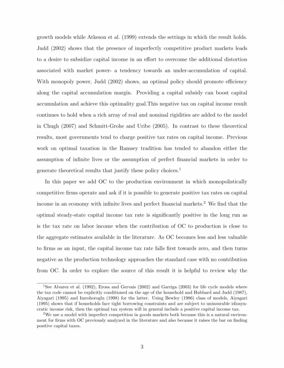
ct : Uct = λt, (5)

nt : −Unt = λt(1− τnt )wt, (6)

kt+1 : λt = βEtλt+1

[(1− τ kt+1)rt+1 + 1− δ

], (7)

bt : λt = βEtλt+1Rt, (8)

tvc : limt→∞

βtλtkt+1 = 0, (9)

tvc : limt→∞

βtλtbt+1 = 0. (10)

Here Uct and Unt are the partial derivatives of U(ct, nt) with respect to ct and nt. The

interpretation of these first order conditions is quite standard. Equation (7) is the

consumption-savings optimality condition. It states that marginal rates of substitution

between present and future consumption equals after-tax return on savings. Equation (7)

implies that capital income tax creates a dynamic distortion in the consumption-savings

margin. Equation (8) determines the gross return on bond holdings. Equations (7) and (8)

imply that after-tax returns on capital and bonds to be equalized each period. Combining

(5) and (6) gives

UltUct

= (1− τnt )wt (11)

Equation (11) gives the optimal labor-leisure choice which is distorted by the tax, τn.

This distortion is purely static in a standard monopolistically competitive model. But, as

will be clear in the next section, in our model the labor income tax also creates a dynamic

distortion.

2.2. The Government

The government faces an exogenous stream of real expenditures that it must finance

through the labor income tax, the capital income tax, and the issuance of real risk-free

one-period debt. Its period-by-period budget constraint is given by

gt +Rt−1bt−1 = bt + τnt wtnt + τ kt rtkt (12)

7

Rt denotes the gross one-period, risk-free, real interest rate in period t. gt denotes per

capita government spending on the final good.

2.3. Production

The production side of the economy builds on earlier work on organizational capital in a

DGE model with monopolistic competition. Following Clarke and Johri (2009) it features

two sectors: an intermediate goods sector that produces differentiated goods using labor,

physical capital and organizational capital, and a final goods sector that uses intermediate

goods to produce a unique final good.

2.3.1. Final Goods Producers

Government consumption goods, private consumption goods and investments are physi-

cally indistinguishable. There are a large number of producers who produce this unique

final good in a perfectly-competitive environment. Final goods producers require only

the differentiated intermediate goods as inputs and use the following CES technology for

converting intermediate goods into final goods.

yt =

[∫ 1

0

yη−1η

it di

] ηη−1

, (13)

where η(> 1) denotes the intratemporal elasticity of substitution across different varieties

of intermediate goods. The differentiated intermediate goods are indexed by i ∈ [0, 1].

Each period final goods firms choose inputs yit for all i ∈ [0, 1] and output yt to

maximize profits given by

yt −∫ 1

0

pityitdi (14)

subject to (13) where pit is the relative price of the ith intermediate good4. The solution

to this problem gives us the input demand functions:

4We normalize the final good’s price, pt, to 1

8

yit = p−ηit (yt). (15)

The zero profit condition can be used to infer the relationship between the final good

price and the intermediate goods prices:

pt(= 1) ≡[∫ 1

0

p1−ηit di

] 11−η

. (16)

2.3.2. Intermediate Goods Producers

There are a large number of intermediate goods producers, indexed by the letter i who

operate in a Dixit-Stiglitz style imperfectly competitive economy. Each of these firms

produces a single variety i using three factor inputs - physical capital, kit, organizational

capital, hit, and labor services, nit. Following Cooper and Johri (2002), the production

technology facing each firm is given by

yit = ztkαitn

1−αit hθit (17)

where yit is the intermediate good variety produced by firm i. The function is assumed

to be concave, and strictly increasing in all three arguments.

The technology differs from a standard neo-classical production function because the

firm carries a stock of OC which is an input in the production technology. Organizational

capital refers to the information accumulated by the firm, through the process of past

production, regarding how best to organize its production activities and deploy its inputs.

As a result, the higher the level of OC, the more productive the firm is. The accumulation

of OC builds on the specification used in Gunn and Johri (2011) and is similar to Chang

et al. (2002), but in addition, we allow for linear depreciation of OC in order to impose

symmetry in the way the two stocks of capital are specified in the model.5

5This symmetry is also a reason why we model OC as accumulating using labor as an input rather

9

We assume that new OC is built using two inputs: labor and old OC. The current

amount of labor used interacts with the existing stock of OC to produce new ideas re-

garding how best to produce goods and this adds to the undepreciated stock of ideas so

that we can write the accumulation equation as:

hi,t+1 = (1− δh)hit + hγitn1−γit , (18)

where δh is the depreciation rate of organizational capital and 0 < δh, γ < 1.6 All pro-

ducers begin life with a positive and identical endowment of organizational capital. The

restriction 0 < δh < 1 is consistent with the empirical evidence supporting the hypoth-

esis of organizational forgetting. Argote et al. (1990) provide empirical evidence for this

hypothesis of organizational forgetting associated with the construction of Liberty Ships

during World War II. Similarly, Darr et al. (1995) provide evidence for this hypothesis

for pizza franchises and Benkard (2000) provides evidence for organizational forgetting

associated with the production of commercial aircraft.

While learning-by-doing is often associated with workers and modeled as the accumula-

tion of human capital, a number of economists have argued that firms are also store-houses

of knowledge. Atkeson and Kehoe (2005) note “At least as far back as Marshall (1930,

bk. iv, chap. 13.I), economists have argued that organizations store and accumulate

knowledge that affects their technology of production. This accumulated knowledge is a

type of unmeasured capital distinct from the concepts of physical or human capital in the

standard growth model”. Similarly Lev and Radhakrishnan (2005) write, “Organizational

capital is thus an agglomeration of technologies, business practices, processes and designs,

including incentive and compensation systems that enable some firms to consistently ex-

tract out of a given level of resources a higher level of product and at lower cost than

than output as in Clarke and Johri (2009).6Note that physical capital accumulation has a symmetric structure. Next period capital is the sum of

the undepreciated stock of physical capital and the new capital produced this period which is a fractionof output, itself produced by a combination of labor and the current stock of physical capital.

10

other firms”. There are at least two ways to think about what constitutes organizational

capital. Some, like Rosen (1972), think of it as a firm specific capital good while others

focus on specific knowledge embodied in the matches between workers and tasks within

the firm. In modeling organizational capital here we follow the second line of thinking.

We assume that the firm must satisfy demand at the posted price. The decision problem

of the firm is to choose plans for nit, kit, hit+1, and pit so as to maximize discounted

life-time profits7:

∞∑t=0

Qt {pityit − wtnit − rtkit}

subject to (17), (18), and (15), where Qt is the appropriate discount factor to use to price

revenue and costs in adjoining periods which is determined in the household problem8.

The first-order conditions associated with the firm’s problem are then:

nit : wt = mcit(1− α)yitnit

+ Ψit(1− γ)n−γit hγit (19)

kit : rt = mcitαyitkit

(20)

hi,t+1 : Ψit = Qt+1Et

[mci,t+1θ

yi,t+1

hi,t+1

+ Ψi,t+1

{(1− δh)

+γhγ−1i,t+1n1−γi,t+1

}](21)

pit : mcit =η − 1

ηpit, (22)

where Ψit and mcit are the Lagrange multipliers associated with the organizational capital

7All input payments are assumed to be made in units of the final good.8Combining (5) and (8) we get the pricing formula for a one-period risk-free real bond

1 = Rtβuc,t+1

uct, which implies the following real pricing kernel between period t and t+ 1:

Qt+1 =βuc,t+1

uct

Consumers discount factor is appropriate to discount period t+1 profit because they own all intermediatefirms and thus receive all the profits.

11

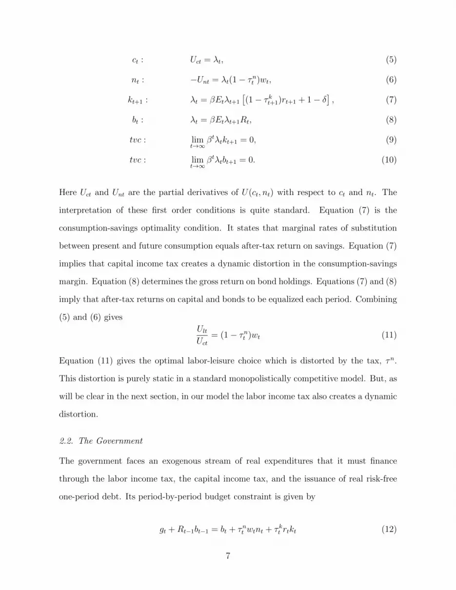
accumulation equation and production function respectively. Equations (20) and (22) are

standard. Equation (21) determines the optimal use of organizational capital by the firm.

One additional unit of organizational capital has a (marginal) value, in terms of profits, of

Ψit to the producer in the current period. The right hand side of (21) measures the value

of having available an additional unit of organizational capital for use by the firm in the

following period. First, the additional organizational capital directly contributes to the

production in the following period as captured by the first term on the right hand side.

Second, the additional organizational capital today has a positive effect on the future stock

of organizational capital which is captured by the two terms inside the curly bracket. First

term is the un-depreciated additional stock and the second term is the new organizational

capital stock generated by this additional stock. In the next period this higher stock of

organizational capital has a marginal value of Ψi,t+1 to the producer. All this must be

discounted by the factor Qt+1. The condition (21) implies that organizational capital will

be accumulated up to the point where the value of an additional unit of organizational

capital today is equal to the discounted value of this organizational capital next period.

The presence of organizational capital dramatically changes a firm’s demand for labor.

Combining (19) and (21) we get:

wt = mcit(1− α)yitnit

+Qt+1

[mci,t+1θ

yi,t+1

hi,t+1

+ Ψi,t+1

{(1− δh) + γhγ−1i,t+1n

1−γi,t+1

}]×(1− γ)n−γit h

γit (23)

The second term on the right hand side of (23) does not appear in a standard model

of monopolistic competition without LBD. In a standard model, a firm’s labor hiring

decision is solely based on the marginal product of labor in the current period. But in

our model, in addition to that basic contribution firms also take into account the positive

effect of an additional unit of labor in accumulating organizational capital in the following

period. One additional unit of labor can generate (1 − γ)n−γit hγit units of organizational

12

capital in the following period. Each of these additional units of organizational capital

has a value of Ψit to the firm. So, the right hand side of (23) gives the total marginal

benefit of having available an additional unit of labor input.

We restrict our attention to a symmetric equilibrium in which all firms make the same

decisions. We thus drop all the subscripts i. That is, in equilibrium yit = yt, cit = ct,

pit = pt = 1, kit = kt, nit = nt, hit = ht and the aggregate production technology and

organizational capital accumulation are given by

yt = ztkαt n

1−αt hθt (24)

ht+1 = (1− δh)ht + hγt n1−γt (25)

We can also aggregate the firm’s optimality conditions, equations (19)- (22), as

wt = mct(1− α)ytnt

+ Ψt(1− γ)n−γt hγt (26)

rt = mctαytkt

(27)

Ψt = Qt+1

[mct+1θ

yt+1

ht+1

+ Ψt+1

{(1− δh) + γhγ−1t+1 n

1−γt+1

}](28)

mct =η − 1

η(29)

2.4. Equilibrium

In the presence of government policy there are many competitive symmetric equilibria, in-

dexed by different government policies. This multiplicity motivates the Ramsey problem.

In our model competitive and Ramsey equilibria are defined as follows:

2.4.1. Competitive Equilibrium

A competitive equilibrium is a set of plans { ct, nt, kt+1, ht+1, it, wt, rt, bt, mct, λt, Ψt, and

Rt}, such that the household maximizes expected lifetime utility taking as given prices

and policies; the firms maximize profit taking as given the wage rate, capital rental rate,

and the demand function; the labor market clears, the capital market clears, the bond

13

market clears, the government budget constraint and the aggregate resource constraint

are satisfied. In other words, all the processes above satisfy conditions (3), (5)-(10), (12),

(24)-(29) and the aggregate resource constraint

ct + gt + it = ztkαt n

1−αt hθt (30)

given policies {τnt , τ kt }, exogenous processes {zt, gt}, and the initial conditions k−1, h−1,

z0, g0.

2.4.2. The Ramsey Equilibrium

The Ramsey equilibrium is the unique competitive equilibrium that maximizes the house-

hold’s expected lifetime utility. Following Schmitt-Grohe and Uribe (2007), we assume

that the benevolent Ramsey planner has been operating for an infinite number of periods

and it honors the commitments made in the past. This form of policy commitment is

known as ‘optimal from the timeless perspective’ Woodford (2003). The Ramsey Equi-

librium is defined as a set of processes ct, nt, kt+1, ht+1, it, wt, rt, τnt , τ kt , bt, mct, λt, Ψt

for t ≥ 0 that maximize:

E0

∞∑t=0

βtU(ct, nt)

subject to the conditions (3), (5)-(10), (12), (24)-(29) and (30), for t > −∞, given

exogenous processes gt and zt, values of all the variables dated t < 0, the values of the

Lagrange multipliers associated with the constraints listed above dated t < 0. Under

traditional Ramsey equilibrium concept, the equilibrium conditions in the initial periods

are different from those applied to later periods. But under Woodford’s timeless definition,

the optimality conditions associated with Ramsey equilibrium are time invariant.

14

3. Parameterization and Solution Method

In order to numerically solve the model, parameter values need to be assigned. We choose

standard values for the parameters used in the business cycle literature and explore how

the optimal tax rates change as the organizational capital parameters vary. The time

unit in our model is one quarter. We set β = .9902 so that the discount rate is 4 percent

(Prescott (1986)) per year. We assume that the period utility function takes the log - log

specification

U(ct, nt) = ln ct + υ ln(1− nt)

The value for υ is set so that the steady state labor supply is 20% in the model without OC.

The exogenous processes for government spending, gt, and productivity, zt, are assumed

to follow independent AR(1) in their logarithms,

ln(gt/g) = ρg ln(gt−1/g) + εgt

ln zt = ρz ln zt−1 + εzt

with εzt ∼ iidN(0, σ2z) and εgt ∼ iidN(0, σ2

g). g is the steady-state level of government

spending and we calibrate this value so that government spending constitutes 17 percent

of steady-state output. We choose the first-order autocorrelation parameters ρz = 0.95

and ρg = 0.85, the standard deviation parameters σz = 0.007 and σg = 0.02 in line with

Chugh (2007) and the RBC literature. Table 2.1 presents the structural parameters used

in the baseline model.

We assign a value of 0.3 to the cost share of capital, α. This is consistent with the

empirical regularity that in developed countries wages represent about 70 percent of total

cost. This brings us to the new parameters associated with organizational capital. Initial

values around which our numerical exercises occur are obtained from the literature. We

set θ = 0.15, γ equal to 0.55. and δ = .025. This value of θ corresponds to a “learning

15

Table 1: Baseline parameter values

Parameters Value Description

β .9902 Subjective discount rateυ 1.913 Labor supply elasticity parameterα 0.3 Share of capital in the production technologyδ 0.025 Depreciation of physical capitalθ 0.15 Elasticity of output with respect to organizational capitalδh 0.025 Depreciation rate of organizational capital

γ 0.55 Org. capital production parameter, ht+1 = (1− δh)ht + hγt n1−γt

g calibrated steady-state level of govt. spendingρg 0.85 persistence in log govt. spending

σεgt 0.02 standard deviation of log govt. spending

ρz 0.95 persistence in log productivityσε

zt 0.007 standard deviation of log productivity

rate”of just under twelve percent and is taken from the lower end of production function

estimates for US manufacturing industries provided in Cooper and Johri (2002). We

studied the response of varying these parameters and found that the results were only

sensitive to θ. These are reported in the next section. To maintain symmetry with the

physical capital we set δh equal to .0259.

We characterize the Ramsey steady-state numerically using the methodology outlined

in Schmitt-Grohe, and Uribe (2005). Their publicly available numerical tools allow the

computation of Ramsey policy in a general class of stochastic dynamic general equilibrium

models.

4. Results

We focus our attention in this section on the long run Ramsey equilibrium without any

uncertainty. After obtaining the dynamic first-order conditions of the Ramsey problem,

we impose the steady state and numerically solve the resulting non-linear system using the

Schmitt-Grohe, and Uribe (2005) algorithm. This gives us the exact numerical solution

9McGrattan and Prescott (2005) use an estimate of 11% (annual rate) for the depreciation rate ofintangible capital which is approximately equivalent to our quarterly value.

16

of the Ramsey problem. After discussing these results we also report the behaviour of

the economy out of steady state as it is hit by shocks to technology and to government

spending.

4.1. Optimal Taxes in the OC Economy

In a standard neoclassical model a capital income tax is worse than a labour income

tax because the former distorts the intertemporal trade-off between current and future

consumption while the latter distorts the static trade-off between consumption and leisure.

A tax on capital income reduces the return to saving and thus affects future consumption

while a tax on current labor income does not have any effect on future consumption,

households work and consume less in the current period.

The presence of organizational capital fundamentally changes this line of reasoning.

Recall that firms combine hours worked with the existing stock of OC to produce ad-

ditional OC which in turn raises the productivity of the firm, giving it the ability to

produce more output without hiring additional physical capital or labor. From the plan-

ners point of view, the additional productivity in the future implies that workers can earn

higher wages and enjoy additional consumption in the future. Anything that reduces the

incentive of the firm to hire labor, in effect, leads to lower accumulation of OC, lower

productivity and therefore lower future consumption. As a result, labor income taxes

affect future consumption in much the same way as capital income taxes do so the plan-

ner is faced with juggling two dynamic distortions in order to achieve the best possible

allocation, which, in general implies positive rates for both taxes.

The relative magnitude of the two tax rates depends on how strongly OC influence

productivity of labor and capital in the production function. This is controlled by the

parameter, θ. Figure 1 plots the value of the optimal tax rates on labor and capital

income chosen by the Ramsey planner as θ is varied from a value of zero to a value of

.15 (which is close to estimates found in the dynamic general equilibrium literature). For

this baseline value of θ, the planner chooses a capital tax rate of 18 percent and a labor

17

Figure 1: OC and optimal tax rates

0 0.02 0.04 0.06 0.08 0.1 0.12 0.14 0.16−0.1

−0.05

0

0.05

0.1

0.15

0.2

0.25

0.3

0.35

0.4

Value of theta

Opt

imal

tax

rate

capital income taxlabor income tax

Student Version of MATLAB

tax rate of 26 percent. As the contribution of OC in output falls (θ is lowered), the tax

rate on labor income rises while that on capital income falls. When OC is no longer part

of the production technology, ( θ = 0), the planner opts for a capital subsidy, in keeping

with earlier results in the literature. We have also explored the impact of varying other

parameters governing the accumulation of organizational capital but the results are barely

sensitive to these parameters so we do not report them here. They are available from the

authors.

Since the OC economy involves increasing returns in the three inputs into production,

a natural question arises: is the positive tax on capital due to increasing returns? We

address this question by solving an economy without OC but with the same degree of

increasing returns in labor and capital as displayed by our baseline OC economy. The

production technology is assumed to be

yit = ztkαitn

1.15−αit . (31)

18

We use (1.15-α) as the labor share so that this model and the OC model have the same

increasing returns in production technology. The representative firm’s problem is to max-

imize profit given by

pityit − wtnit − rtkit (32)

subject to (31) and (15). The first order conditions associated with this problem are then:

nit : wt = mcit(1.15− α)yitnit

(33)

kit : rt = mcitαyitkit

(34)

pit : mcit =η − 1

ηpit, (35)

We impose symmetry in the production sector and solve the Ramsey problem for this

economy using the same baseline parameter values described in section 2.3. The resulting

solution gives us the following optimal tax rates:

τ k = −0.3, τn = 0.42

Clearly then, merely introducing increasing returns in production cannot account for

positive taxation of capital income.

4.2. Ramsey Dynamics

Having discussed the steady state properties of the model with OC we turn to the response

of the planner to technology and government spending shocks. We compute the numerical

solution to the Ramsey problem based on a second-order approximation of the Ramsey

planner’s decision rules. We approximate the model in levels around the non-stochastic

steady-state based on the perturbation algorithm described in Schmitt-Grohe and Uribe

(2004a). As in Schmitt-Grohe and Uribe (2004b), we first generate simulated time series

of length 100 for the variables of interest and then compute the first and second moments.

We repeat the procedure 500 times and report the averages of the moments.

19

Table 2 displays the usual moments reported in the Ramsey taxation literature. While

the presence of OC leads to amplification of shocks so that output varies more than in a

corresponding model without OC, much of the basic features of taxation carry through

to this economy. Supporting results in Chari et al. (1994); Chugh (2007), the tax rate

on labor income fluctuates very little but capital income tax is relatively volatile. Since

these are already discussed in the literature, we keep our discussion short. The planner

chooses to smooth the labor income tax while using the capital income tax for consumption

smoothing purposes. As a result the capital tax varies considerably around its mean value

of .18.

Table 2: Dynamic properties of Ramsey allocation

Variable Mean Std. Dev. Auto. corr. Corr(x,y) Corr(x,g) Corr(x,z)

Ramsey model with OCτn 0.2552 0.0061 0.9091 -0.9994 -0.0737 -0.9876τ k 0.1855 0.1686 -0.0070 0.1098 0.5137 0.0584R− 1 4.0019 0.0007 0.8712 0.5912 0.2568 0.6472y 4.5332 0.0884 0.9066 1.0000 0.0919 0.9876n 0.2792 0.0035 0.8624 0.8490 0.4022 0.8473i 0.6632 0.0600 0.8545 0.7874 -0.3928 0.8713c 2.9615 0.0465 0.9650 0.7530 -0.3326 0.7389

Ramsey model without OCτn 0.4325 0.0007 0.8477 -0.2182 -0.8863 0.0472τ k -0.1377 0.2000 -0.0121 -0.1303 0.3816 -0.2480R− 1 4.0007 0.0007 0.9287 -0.0796 0.5034 -0.2537y 0.3625 0.0073 0.8850 1.0000 0.2784 0.9513n 0.1987 0.0020 0.8477 0.2182 0.8863 -0.0472i 0.0369 0.0024 0.8053 0.7073 -0.2376 0.8099c 0.2530 0.0053 0.9340 0.8329 -0.2121 0.9489

Note: The net real interest rate, R − 1, is expressed in percent peryear.

5. Conclusion

We introduce organizational capital and imperfect competition into an otherwise stan-

dard infinite horizon dynamic general equilibrium model in order to study the properties

20

of optimal taxation in the Ramsey tax framework. Our numerical solutions suggest that

while the introduction of monopoly power calls for a capital income subsidy, the intro-

duction of organizational capital creates a stronger incentive to tax capital income. In

our model, both capital and labor income tax distort the dynamic trade-off between cur-

rent consumption and future consumption. Consequently, it is optimal for the Ramsey

planner to tax both capital income and labor income. The relative magnitudes of the tax

rates depend crucially on the contribution of organizational capital to output, in firms

production technology.

References

Aiyagari, S.R., 1995. Optimal capital income taxation with incomplete markets, borrowing

constraints, and constant discounting. Journal of Political Economy 103, 1158–75.

Alvarez, Y., Burbidge, J., Farrell, T., Palmer, L., 1992. Optimal taxation in a life-cycle

model. The Canadian Journal of Economics / Revue canadienne d’Economique 25,

111–122.

Argote, L., Beckman, S.L., Epple, D., 1990. The persistence and transfer of learning in

industrial settings. Management Science 36, 140–154.

Atkeson, A., Chari, V., Kehoe, P.J., 1999. Taxing capital income: a bad idea. Quarterly

Review , 3–17.

Atkeson, A., Kehoe, P.J., 2005. Modeling and measuring organization capital. Journal of

Political Economy 113, 1026–1053.

Benkard, C.L., 2000. Learning and forgetting: The dynamics of aircraft production.

American Economic Review 90, 1034–1054.

21

Bewley, T.F., 1986. Stationary monetary equilibrium with a continuum of independently

fluctuating consumers, in: Hildenbrand, W., Mas-Colell, A. (Eds.), Contributions to

Mathematical Economics in Honor of Gerard Debreu. Amsterdam: North-Holland.

Chamley, C., 1986. Optimal taxation of capital income in general equilibrium with infinite

lives. Econometrica 54, 607–22.

Chang, Y., Gomes, J.F., Schorfheide, F., 2002. Learning-by-doing as a propagation mech-

anism. American Economic Review 92, 1498–1520.

Chari, V.V., Christiano, L.J., Kehoe, P.J., 1994. Optimal fiscal policy in a business cycle

model. Journal of Political Economy 102, pp. 617–652.

Chugh, S.K., 2007. Optimal inflation persistence: Ramsey taxation with capital and

habits. Journal of Monetary Economics 54, 1809–1836.

Clarke, A.J., Johri, A., 2009. Procyclical solow residuals without technology shocks.

Macroeconomic Dynamics 13, 366–389.

Cooper, R., Johri, A., 2002. Learning-by-doing and aggregate fluctuations. Journal of

Monetary Economics 49, 1539–1566.

Darr, E.D., Argote, L., Epple, D., 1995. The acquisition, transfer, and depreciation of

knowledge in service organizations: productivity in franchises. Management Science 41,

1750–1762.

Erosa, A., Gervais, M., 2002. Optimal taxation in life-cycle economies. Journal of Eco-

nomic Theory 105, 338–369.

Gunn, C., Johri, A., 2011. News and knowledge capital. Review of Economic Dynamics

14, 92–101.

22

Hubbard, R.G., Judd, K.L., 1987. Social security and individual welfare: Precautionary

saving, borrowing constraints, and the payroll tax. American Economic Review 77,

630–46.

Johri, A., 2009. Delivering endogenous inertia in prices and output. Review of Economic

Dynamics 12, 736–754.

Johri, A., Lahiri, A., 2008. Persistent real exchange rates. Journal of International

Economics 76, 223–236.

Johri, A., Letendre, M.A., Luo, D., 2011. Organizational capital and the international

co-movement of investment. Journal of Macroeconomics 33, 511 – 523.

Jones, L.E., Manuelli, R.E., Rossi, P.E., 1997. On the optimal taxation of capital income.

Journal of Economic Theory 73, 93–117.

Judd, K.L., 1985. Redistributive taxation in a simple perfect foresight model. Journal of

Public Economics 28, 59–83.

Judd, K.L., 2002. Capital-income taxation with imperfect competition. American Eco-

nomic Review 92, 417–421.

Lev, B., Radhakrishnan, S., 2005. The valuation of organization capital, in: Measur-

ing Capital in the New Economy. National Bureau of Economic Research, Inc. NBER

Chapters, pp. 73–110.

Marshall, A., 1930. Princeples of Economics: An Introductory Volume. London: Macmil-

lan.

McGrattan, E.R., Prescott, E.C., 2005. Taxes, regulations, and the value of u.s. and u.k.

corporations. Review of Economic Studies 72, 767–796.

Prescott, E.C., 1986. Theory ahead of business cycle measurement. Technical Report.

23

Prescott, E.C., Visscher, M., 1980. Organization capital. The Journal of Political Economy

88, 446–461.

Rosen, S., 1972. Learning by experience as joint production. The Quarterly Journal of

Economics 86, 366–82.

Schmitt-Grohe, S., Uribe, M., 2004a. Optimal fiscal and monetary policy under imperfect

competition. Journal of Macroeconomics 26, 183 – 209.

Schmitt-Grohe, S., Uribe, M., 2004b. Solving dynamic general equilibrium models using

a second-order approximation to the policy function. Journal of Economic Dynamics

and Control 28, 755 – 775.

Schmitt-Grohe, S., Uribe, M., 2005. Optimal fiscal and monetary policy in a medium-scale

macroeconomic model. NBER Macroeconomics Annual 20, 383–425.

Schmitt-Grohe, S., Uribe, M., 2007. Optimal simple and implementable monetary and

fiscal rules. Journal of Monetary Economics 54, 1702 – 1725.

Woodford, M.D., 2003. Interest and Prices. Princeton University Press: Princeton, New

Jersey.

24