1

Taxation-Based Stabilization Policy

Bernhard Herza Werner Roegerb* Lukas Vogela

Preliminary version

May 2004

1. Introduction

As countries enter currency unions or fixed exchange rate regimes they loose their monetary

independence. The costs and benefits of giving away monetary policy have been comprehen-

sively discussed in the context of European Monetary Union. Asymmetric shocks and poten-

tial differences in the monetary policy transmission increase the importance of and the re-

quirements for national fiscal policy as a tool for macroeconomic stabilization in the Euro

area. This stabilization role conflicts with serious provisos against fiscal policy activism,

however. Political economy incentives can substantially impair the anti-cyclical use of fiscal

policy. Additionally, the potential deficit bias puts the long-run sustainability of government

budgets at risk. Hence there seems to be a need for implementable fiscal policy rules.

In the context of this discussion, the paper investigates the potential for rule-based fiscal stabi-

lization policy in a monetary union. The analysis uses a small dynamic optimising agent

specification that is a standard tool in monetary policy research. We build on the models of

Clarida et al. (2001), Galí and Monacelli (2002) and McCallum and Nelson (1997), and re-

strict attention to the small open economy case. We modify the aggregate demand equation to

examine the stabilizing potential of fiscal policy and focus on the revenue side of the budget.

Specifically, we explore the stabilizing potential of variable tax rates. Thus, the analysis treats

fiscal policy as an endogenous variable and not as an exogenous shock as in the conventional

analysis of (monetary) stabilization policy.

a VWL 1, Economics Department, University of Bayreuth, Germany (corresponding author: lukas.vogel@uni-bayreuth.de, Tel.: +49-921-55.29.14) b European Commission, DG ECFIN * The views expressed in this paper are those of the authors only.

2

While monetary policy has several advantages as a stabilization tool, e.g. the short decision

lags and the reversibility of interest rate decisions (Taylor 2001), there are also certain limita-

tions. In particular, monetary policy cannot react to asymmetric shocks in a monetary union.

Against this background, the paper adapts the discussion of monetary policy to the question of

taxation-based stabilization. To this aim, we replace the interest rate rule by a tax rule. The

basic idea is that time-varying tax rates can be an adequate tool for stabilizing, anti-cyclical

fiscal policy. The focus of this paper is on taxing consumption. Looking at taxation instead of

time-varying expenditure can be justified by efficiency arguments. Mountford and Uhlig

(2002) argue that, in the U.S., deficit-financed tax reductions have been superior to deficit- or

tax-financed expenditure increases as a macroeconomic stabilization tool. Wijkander and

Roeger (2002) furthermore suggest that variations in the VAT have a relatively strong effect

on aggregate demand.

In contrast to much of the literature on macroeconomic stabilization, we do not restrict the

role of fiscal policy to the operating of automatic stabilizers. The motivation is twofold.

Firstly, automatic stabilizers dampen macroeconomic shocks only partially (Calmfors 2003),

so that discretionary action may add to the stabilizing potential. Secondly, although automatic

stabilizers certainly succeed in smoothen cyclical fluctuations, they may face a trade-off be-

tween allocation efficiency and macroeconomic stabilization. Their stabilizing potential is

higher the more progressive the tax system and the more generous the transfer payments to

the unemployed (Buti and Van den Noord 2003).

The analysis presumes that fiscal policy in the form of time-varying taxation has a priori no

disadvantage with regard to the decision lag and the reversibility of decisions, i.e., we assume

that the variable tax component can be adjusted at a similar speed as interest rates in monetary

policy. Considering the present fiscal constitution of EMU member states this assumption is

obviously too restrictive. Therefore, the discussion about fiscal stabilization policy also has to

include institutional reforms. The proposals range from improved transparency and rules for

national governments to the idea of delegating fiscal stabilization policy to an independent

agency (Calmfors 2003, Wyplosz 2001).

The following section presents variable taxation in a dynamic model of optimising house-

holds. Section three then discusses the impact of inflation in the model. In section four, we

calibrate the model equations and simulate impulse responses. Section five summarizes the

main findings and concludes.

3

2. Model

This section incorporates fiscal policy in a dynamic model of inter-temporally utility maxi-

mizing households. Thereby, the focus is on time-varying taxation. This aspect of fiscal pol-

icy is made endogenous. The aim is to investigate its potential for macroeconomic stabiliza-

tion in the absence of monetary policy. The discussion rests upon the model of Clarida et al.

(2001) and Galí and Monacelli (2002). It simplifies the latter by restricting attention to coun-

tries within a monetary union. In such a setting, we do not have to consider nominal exchange

rates and their impact on the terms of trade. On the other hand, we extend the small open-

economy specification by including time-varying taxation as a policy tool. We consider a

component τ of the VAT that may be adjusted according to the objective of output stabiliza-

tion. In equilibrium, this component is equal to zero. The deviation of the tax rate τ from its

steady state value thus simplifies to ttt ττττ =−=ˆ . As we consider distortionary taxation,

the proposition of Ricardian equivalence does not hold.

This section proceeds by presenting the building blocks of the model. We first discuss house-

hold utility. Then we derive aggregate demand. As third element we introduce the inflation

dynamics and, finally, discuss the fiscal policy rule.

2.1 Household utility

The model focuses on the behaviour of a representative agent or representative household.

Household utility is given as the discounted stream of utility

(1) ∑∞

=+=

0jjt

jt UEU β ,

with β as the discount factor.

Household utility is a function of household consumption and leisure. The positive valuation

of leisure implies that working negatively affects household utility. With overall utility being

additive in the utility of consumption and the disutility of working we get

(2) φσ

φσ+−

+−

−= 11

11

11),( ttttt NCNCU ,

where C is consumption, N is the time spent working, σ is the coefficient of relative risk

aversion, or the inverse of the inter-temporal elasticity of substitution, and φ is the inverse of

the elasticity of labour supply.

4

Households consume a basket of domestic and foreign goods and services. We assume that

the partition of consumption in foreign and domestic commodities can be described by the

following CES utility function (see Galí and Monacelli 2002)

(3) 11

,

11

,

1

)1(−−−

+−=

ηη

ηη

ηηη

η αα tFtHt CCC ,

with HC and FC as domestic and imported consumer goods, respectively, η as the elasticity

of substitution between HC and FC , and α as the equilibrium share of imports in domestic

household consumption.

The private sector’s budget constraint is

(4) tt

ttttFtFttHtHtttt B

iBXPCPCPTNW −+

+−+++≥− +

1)1()1( 1

,,,, ττ .

Note that, in order to keep the argument simple, capital and investment in capital is omitted in

the model. Since our focus is on the effects of taxing consumption, this simplification seems

admissible at this stage. Whether, or under which conditions, investment may be affected in

an indirect or second round effect via the real interest rate changes is an aspect for further in-

vestigation.

The elements in the above restriction are the nominal wage per unit of labour, tW , the expen-

diture on domestic consumer goods, tHtHt CP ,,)1( τ+ , the spending on foreign consumer

goods, tFtFt CP ,,)1( τ+ , the exports of domestically produced commodities, tt XP , and the in-

vestment in risk-free one-period bonds, ttt BiB −++ )1/(1 . The nominal interest rate is ti . Be-

cause labour is the only factor of production, all income from production is paid as wages.

The government collects lump-sum taxes tT to finance public spending.

Consumption is taxed in the country of destination at the rate tτ . Therefore, the overall spend-

ing of domestic households on consumer goods is tFtFttHtHt CPCP ,,,, )1()1( ττ +++ . The term

tttFtFt XPCP −+ ,,)1( τ , on the other hand, can be considered as the private sector net imports.

The representative agents maximize utility as given in (1) to (3) under the budget constraint

(4). For household consumption, the resulting first order conditions are

(5) tttt PC )1( τλσ +=−

5

(6) 1111 )1( +++−+ += tttt PC τλσ

Maximizing utility from consumption according to (3) and (4), the shares of domestic and of

imported commodities in tC equal

(7) tt

tHtH C

PP

Cη

α−

−= ,

, )1( tt

tFtF C

PP

Cη

α−

= ,

, ,

and the resulting price level is

(8) ( ) ηηη αα −−− +−= 11

1,

1,]1[ tFtHt PPP .

The first order condition for labour supply is

(9) ttt WN λφ = ,

and for saving in one-period bonds

(10) 1)1( ++= ttt i λβλ .

Plugging (5) and (6) into (10), one obtains the equation for the inter-temporal trade-off be-

tween saving and consumption

(11)

++

+=

++

−

+

11

1

)1()1()1(1

tt

tt

t

ttt P

PC

CEiτ

τβσ

.

With XXx tt lnlnˆ −= as the percentage deviation of variable tX from its steady state X ,

xx ≈+ )1ln( for x close to zero, and 1)1( −−= rβ , we obtain the standard log-linear ap-

proximation of the Euler equation (11) around the steady state, extended by the inclusion of

the variable consumption tax

(12) )(1ˆˆ 111 rEEicEc ttttttttt −−−+−= +++ πττσ

.

The trade-off between consumption and leisure determines labour supply according to (5) and

(9) as

(13) tt

t

t

t

PW

CN

)1( τσ

φ

+=− ,

6

which states that labour supply is a function of the real wage. The higher the consumer tax

rate, the lower the real wage. In logarithmic form, with smaller case letters as the variables’

logarithms, the equation becomes

(14) ttttt cnpw σφτ +=−− .

2.2 Aggregate demand

Let us now define aggregate demand for domestically produced goods and services as

(15) ttHtHt GCCY ++= *,, .

Its log-linear approximation around the steady state is

(16) ttHtHt gYGcc

YCy ˆ)ˆˆ]1([ˆ *

,, ++−= αα ,

where YC / is the steady-state share of consumer goods in total demand, which combines

)/)(1( YCα− , the share of domestic households, and )/( YCα , the share of exports in overall

demand. A star indicates the variables of the foreign country, or, more accurately, for the ag-

gregate of foreign countries. Finally, G is government consumption of domestically produced

commodities. It is financed by the lump-sum tax T and considered exogenous. For simplicity,

we further assume that government spending prevails at its equilibrium level, so that 0ˆ =g .

Similarly, the log-linear approximation of domestic household consumption, tFtHt CCC ,, += ,

around the steady state is

(17) tFtHt ccc ,, ˆˆ)1(ˆ αα +−= .

The analogous expression for foreign household consumption is

(18) *,

*,

* ˆˆ)1(ˆ tHtFt ccc γγ +−= ,

with γ as the share of domestic country exports in foreign household consumption. Because

we assume the domestic country to be small compared to the aggregate of remaining EMU

countries, the share γ in overall foreign household consumption is negligible.

Inserting (17) in (16), assuming 0ˆ =g , and re-arranging the terms, one obtains

(19) ])ˆˆ[]ˆˆ[ˆˆ]1([ˆ ,**

,*

ttFttHttt ccccccYCy −−−++−= αααα .

7

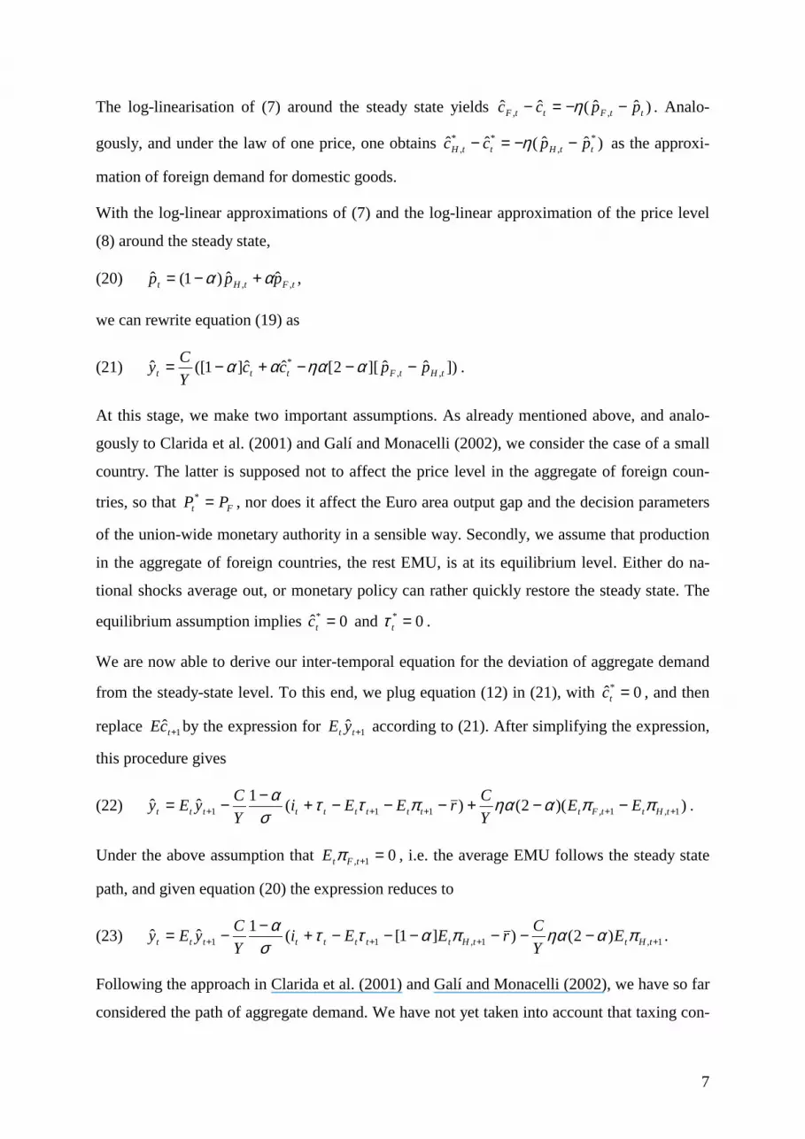
The log-linearisation of (7) around the steady state yields )ˆˆ(ˆˆ ,, ttFttF ppcc −−=− η . Analo-

gously, and under the law of one price, one obtains )ˆˆ(ˆˆ *,

**, ttHttH ppcc −−=− η as the approxi-

mation of foreign demand for domestic goods.

With the log-linear approximations of (7) and the log-linear approximation of the price level

(8) around the steady state,

(20) tFtHt ppp ,, ˆˆ)1(ˆ αα +−= ,

we can rewrite equation (19) as

(21) ])ˆˆ][2[ˆˆ]1([ˆ ,,*

tHtFttt ppccYCy −−−+−= αηααα .

At this stage, we make two important assumptions. As already mentioned above, and analo-

gously to Clarida et al. (2001) and Galí and Monacelli (2002), we consider the case of a small

country. The latter is supposed not to affect the price level in the aggregate of foreign coun-

tries, so that Ft PP =* , nor does it affect the Euro area output gap and the decision parameters

of the union-wide monetary authority in a sensible way. Secondly, we assume that production

in the aggregate of foreign countries, the rest EMU, is at its equilibrium level. Either do na-

tional shocks average out, or monetary policy can rather quickly restore the steady state. The

equilibrium assumption implies 0ˆ* =tc and 0* =tτ .

We are now able to derive our inter-temporal equation for the deviation of aggregate demand

from the steady-state level. To this end, we plug equation (12) in (21), with 0ˆ* =tc , and then

replace 1ˆ +tcE by the expression for 1ˆ +tt yE according to (21). After simplifying the expression,

this procedure gives

(22) ))(2()(1ˆˆ 1,1,111 +++++ −−+−−−+−−= tHttFtttttttttt EEYCrEEi

YCyEy ππαηαπττ

σα .

Under the above assumption that 01, =+tFtE π , i.e. the average EMU follows the steady state

path, and given equation (20) the expression reduces to

(23) 1,1,11 )2()]1[(1ˆˆ ++++ −−−−−−+−−= tHttHtttttttt EYCrEEi

YCyEy παηαπαττ

σα .

Following the approach in Clarida et al. (2001) and Galí and Monacelli (2002), we have so far

considered the path of aggregate demand. We have not yet taken into account that taxing con-

8

sumer goods creates a wedge between aggregate spending and effective aggregate demand.

This distinction shall be discussed in the following.

Private households are, in the first place, constrained in their overall expenditure. Equation (4)

states that overall private consumption expenditure in t cannot exceed the wage earned plus

the dissaving minus the lump-sum taxes paid over this period. Therefore, the household prob-

lem of inter-temporal optimisation in equation (12) is, in the first place, above the inter-

temporal allocation of consumption expenditure. In this context, the Euler equation gives an

optimum for the ratio of present to future consumption. It does, however, not specify the

absolute levels of present and future demand.

From equation (15) we have the level of effective demand for domestic products as

ttHtHt GCCY ++= *,, . Overall spending on domestically produced commodities, the element

fixed by the budget constraint, on the other hand is

(24) ttHtHtt GCCZ +++= *,,)1( τ

The wedge between overall spending and aggregate demand is thus tHttt CYZ ,τ=− . As

above, we assume the aggregate of foreign economies to operate on the equilibrium path. This

implies that 0* =tτ and avoids complications from tax-driven fluctuations in export demand.

What households can actually smooth independently is the inter-temporal allocation of con-

sumption expenditure, i.e. of ttt CC )1( ττ += . We may thus rewrite equation (12) as the inter-

temporal allocation of consumer spending as

(25) )(1ˆˆ 111 rEEicEc ttttttttt −−−+−= +++ πττσ

ττ ,

with ttt cc ττ += ˆˆ . The log-linear approximation of (24) around the steady state yields

(26) ttHtHt gYGcc

YCz ˆ)ˆˆ]1([ˆ *

,, ++−= αα τ ,

because YZ = holds in the steady state. For the difference between the overall demand and

the overall expenditure deviation from the steady state it follows

(27) ttt YCzy τα )1(ˆˆ −−= .

Analogously to (23) we can write the optimising equation for aggregate expenditure on do-

mestically produced commodities as

9

(28) tztHttHtttttttt EYCrEEi

YCzEz ,1,1,11 )2()]1[(1ˆˆ επαηαπαττ

σα +−−−−−−+−−= ++++ ,

where we have added tz ,ε as a demand shock. Finally, we thus obtain the deviation of aggre-

gate demand from its equilibrium level as

tztHttHtttttttt EYCrEEi

YCzEy ,1,1,11 )2()]1[]1[(1ˆˆ επαηαπαττσ

σα +−−−−−−++−−= ++++ .

2.3 Aggregate supply and inflation dynamics

In the absence of monetary or fiscal policy intervention, the model dynamics is entirely driven

by the interaction of inflation and the output gap in reaction to exogenous shocks. The impact

of inflation on the output gap has been derived in the above sections. This section sketches out

the effect of aggregate demand on inflation.

We suppose that fluctuations in aggregate supply are, in the short run, determined by fluctua-

tions in aggregate demand. Any quantity demanded can be supplied. However, we do not as-

sume that they are supplied at constant costs. Instead, marginal costs are supposed to vary

with fluctuations in the level of production. The deviations of output from its steady state are

thus associated with price level changes or inflation. As we are concerned with the output gap

of the domestic economy, we focus on the price level for domestically produced commodities.

According to standard practice, firms are considered as setting their prices in a forward-

looking manner and as charging a fixed price mark-up. Under the assumption of staggered

price setting, the New Keynesian Phillips curve (see e.g. Clarida et al. 1999, Galí and Mona-

celli 2003, Galí 2003) results as

(29) ttHttH cmE ˆ1,, λπβπ += + .

The point now is to relate the log-deviations of domestic real marginal costs from their equi-

librium level to the domestic output gap. To this aim, the logarithm of real marginal costs can

be expressed as

(30) ttHtt apwmc −−= , ,

where ta is the parameter of labour productivity. Inserting the labour supply equation (14),

one can rewrite the expression as

tttHtttt appncmc −+−++= τφσ )( , .

10

Above we assumed, that output is determined by aggregate demand, in the short run. As la-

bour is the only factor of production, the production function is ttt NAY = . In logarithmic

terms this gives ttt nay += , so that

(31) tttHtttt appycmc )1()( , φτφσ +−+−++= .

From the fact that the steady-state consumption equation (11) holds for domestic and foreign

households, and assuming an integrated bond market, Galí and Monacelli (2002, 6) derive

)(1,,

*tHtFtt ppcc −

−+=σ

α

as log-relationship between domestic and foreign consumption. Together with equation (7) for

tHC , and *,tHC , they furthermore obtain (see Galí and Monacelli 2002, 9f.)

)()1)(2(1

)( *,, tttHtF yypp −

−−+=−

σηαασ .

Using )( ,,, tHtFtHt pppp −=− α from (20), replacing tc and tHtF pp ,, − in (31) by the two

above expressions, and assuming that the aggregate of foreign countries operates at the

steady-state level, with 0ˆ* =tc and 0ˆ * =ty , the deviation of marginal costs from steady state

are equal to

(32) tttt aycm ˆ)1(ˆ)1)(2(1

ˆ φτφσηαα

σ +−+

+−−+

= ,

where tt ua ++− ˆ)1( φλ can be replaced by t,πε to indicate a technology or cost shock. The

component tu is a cost-push shock that can be motivated, e.g., by adding a wage mark-up at

the right-hand side of equation (14). Insertion of (32) and the cost shock in (29) finally gives

the reaction of inflation to the output gap as

(33) ttttHttH yE ,1,, ˆ)1)(2(1 πελτφ

σηαασλπβπ ++

+−−+

+= + .

Although appealing as a theoretical benchmark, equation (33) has been contested on empirical

grounds. The reason is the observed persistence of inflation rates (see Galí et al. 2001). There

seems to be an important autoregressive component in price level changes. This inflation iner-

tia is captured by the so-called hybrid Phillips curve, which is

ttHtHttH cmE ˆ)1( 1,1,, λβπρπρβπ +−+= −+ ,

11

with 10 << ρ . Replacing the marginal cost component as above, we then obtain inflation in

the price level of domestic goods as

(34) ttttHtHttH yE ,1,1,, ˆ)1)(2(1

)1( πελτφσηαα

σλπρπρβπ ++

+−−+

+−+= −+ .

2.4 Fiscal policy

As a final component, we add the fiscal policy rule. The notion of fiscal rules appears in dif-

ferent connotations in the literature. Often it explicitly refers to legally enshrined limitations

on fiscal policy discretion. Here, we refer to fiscal rules as a reaction function for the policy

maker, analogously to rules in monetary policy. The fiscal policy rule is thus meant to guide

the action of the fiscal authority.

The policy variable to be adjusted is a mark-up on the consumer tax. So, which are the argu-

ments to guide the policy choice? With output and employment stabilization as an obvious

goal, one should include the output gap. The variable tax component should be lowered in re-

sponse to negative and raised in reaction to positive deviations of production from its poten-

tial level. The argument seems also justified on empirical grounds. Bohn (1998), for the U.S,

and Ballabriga and Martinez-Mongay (2002), for the EU members, find evidence for an anti-

cyclical reaction of fiscal deficits. Galí and Perotti (2003) conclude that the objective of out-

put stabilization has gained importance in the EU countries’ fiscal policies since 1992.

Thereby, the anti-cyclical reaction comes not only from the automatic stabilizers, but it also

extents to discretionary policy action.

A second point is whether the policy rule should also contain an inflation-stabilization objec-

tive. The principal objection is that the ECB policy target pins down the long-run national in-

flation rate. An additional national inflation target would only be a target for relative price

level developments in the euro area. Fiscal policy should therefore content itself to output sta-

bilization (Calmfors 2003). Additionally, a numerical target for the inflation level would de-

prive the government of its degree of freedom, as its action would then also depend on the

central bank’s target level and on the realisation of the latter.

One argument in favour of a national inflation target is that the welfare costs from inflation

accrue irrespective to whether other countries are affected in a similar way or not. A second

one relates to the real interest rate effect (e.g. Bofinger 2003). In our model, the nominal in-

terest rate is exogenous. The real interest rate thus varies with expected changes in the price

level. National inflation differentials then imply country differences in the real interest rate. In

12

the above aggregate demand equation, lower real rates induce households to shift consump-

tion from the future to the present. The result is an increasing output gap, which by itself posi-

tively affects current inflation. In the open economy this effect is at least partially compen-

sated. Increasing expected inflation here leads to a decline in net exports, which negatively

affects aggregate demand. However, for a certain combination of parameters the export effect

seems too week to counter the real interest rate effect of inflation (see section 3).

In order not to preclude the relevance of the latter arguments, we specify the tax rule as

(35) ttHtt y ,,ˆ τεκπµτ ++= ,

with 0>µ , 0≥κ , and with t,τε as non-systematic variation in the tax component. The pol-

icy rule is fairly simple. Under temporary and randomly distributed shocks, it is also compati-

ble with the sustainability of public finances. If government revenue is equal to government

expenditure in equilibrium, the revenue from taxation will fall short of expenditures in reces-

sions and exceed government spending in booms. The steady-state level of the variable tax

component is zero, as is the average amount of extra VAT paid over the business cycle.

Beside this compatibility, the solvency requirement may also suggest to consider the overall

level of debt relative to GDP as a third element in the tax rule (35). A high level of debt

should then lead to tax increases in order to collect additional revenue. However, debt stabili-

sation can also be achieved by adapting other sources of government income. An option is to

adjust lump-sum taxes, as in Perez and Hiebert (2002), instead of charging the variable VAT

component with a double objective.

Finally, research on monetary policy has proposed some modifications on reaction function

such as equation (35). These extensions include interest rate or tax smoothing, the use of

lagged or of expected values for the output gap and inflation, and the replacement of the out-

put gap by GDP growth (see Schmitt-Grohe and Uribe 2003). Such modifications may be

considered such modifications in subsequent work. To keep the focus on our key question,

they are however excluded for the time being.

3. The impact of inflation: expansionary or contracting?

We have already mentioned in section 2.4 that the qualitative impact of expected inflation on

the output path depends on the model calibration. To see this, consider the effect of inflation

in the unregulated system, i.e. in a situation without policy reaction. An expected increase in

13

the price level lowers the real interest rate, which has an expansionary effect. But above-

average national inflation rates do, on the one hand, also reduce net exports. Whether the lat-

ter can neutralize the expansionary impact of the real interest rate effect depends on the de-

gree of economic openness, on the inter-temporal elasticity of substitution and on the elastic-

ity of substitution between domestic and foreign commodities. The output-gap equation (23)

illustrates the argument. Without the tax variable, it can be re-formulated as

)(1]2[)1(ˆˆ2

1,1 riYC

YCEyEy ttHtttt −−−

−−−+= ++ σ

ααηασαπ .

For inflation to have a contracting impact on the output gap, price level increases should

dampen aggregate demand. The latter requires the term in brackets to become negative. This

is equivalent to

σααηα

2)1()2( −>− ,

which gives

01

122 >+

+−ησ

αα .

As 10 << α , the relevant solution is

21

11

+−>

ησησα .

For common parameter choices, 5.0=η and 1=σ , this implies 42.0>α . Thus, for a steady-

state degree of economic openness smaller 0.42, the expansionary real interest rate effect pre-

vails, whereas in a more open country the dampening impact on net exports dominates the

dynamics.

4. Simulation results

The following section presents initial results from model simulations with the tax rule (35) in

the context of the above model, consisting of equations (27), (28) and (33). In order to simu-

late impulse responses, the equations have to be calibrated. Table 1 contains the parameter

14

values assigned. For the smaller EMU countries, the overall share of consumption in GDP and

the ratio of exports to GDP are both about 0.55 (European Commission 2003).1

Together with the above demand specification, which assumes that only consumption goods

are traded, it follows that )/( YGα is roughly 0.30, and )/)(1( YGα− is about 0.25. Common

choices for σ are 1 (Clarida et al. 2000) or 2. The elasticity of substitution between exports

and imports, η , is the weighted average for the EMU countries in Fagan et al. (2001). For the

impact of marginal cost fluctuations on inflation and for inflation persistence, we follow the

Euro area estimates of Galí et al. (2001). The nominal interest rate is set exogenously at

rit = .

YC / α σ η β λ ρ φ µ κ

0.55 0.55 1.00 0.50 0.99 0.09 0.70 1.00 0.10; 1.0; 2.0 0.00

Table 1: Model calibration

As indicated above, this section limits itself to impulse responses from the purely forward-

looking model, i.e. to a model without inflation or output-gap persistence. We present results

from two different simulation scenarios. The first one considers impulse responses to a persis-

tent unit demand shock, with an AR (1) coefficient in the shock of 0.95. The second simula-

tion looks at the system’s behaviour after a persistent unit supply shock, with an AR (1) coef-

ficient of 0.95. The simulations are deterministic ones. We investigate the path towards the

steady state after the economy has been hit by the unit shock in period one. The paths of the

variables are given in percentage-point deviations from their respective equilibrium or flexi-

ble-price levels. Each period corresponds to a quarter of a year.

We are interested in investigating the stabilizing potential of the consumer-tax rule. To this

aim, and as a first step, we consider the policy implications and the system dynamics under

different sensitivities of the policy instrument to the output gap. More precisely, given the rule

ttHtt y ,,ˆ τεκπµτ ++= , we compare the impulse responses for 0=κ and 0.2;0.1;1.0=µ .

Equations (27) and (28) together with the policy rule suggest that the stabilization becomes

more difficult the higher the persistence of shocks. The reason is that for the consumption tax

to bring about shifts in the inter-temporal allocation of consumption expenditure what matters

1 These are non-weighted average values for Austria, Belgium, Greece, Finland, Ireland, the Netherlands and Portugal.

15

is the difference between the actual and the expected future tax rate. Focusing on the situation

of high shock persistence, the simulation thus considers something like a worst-case scenario

for the discussed stabilization tool.

Although discussing monetary policy at the country level is counterfactual in the context of a

monetary union or a fixed exchange rate regime, we finally look at the stabilizing potential of

monetary policy following an equivalent monetary policy rule. As the transmission of mone-

tary policy differs from the one of distortionary taxation in our model, this comparison is a

very informal one. It only aims at giving some qualitative indications as to whether there are

marked differences between the stabilizing potential of fiscal and monetary policy under the

above economic structure. Additionally, the annex contains the impulse responses for the un-

regulated system. They show that the implementation of the fiscal rule makes a difference

compared to the unregulated system, at least if the sensitivity of taxation to the output gap in

the former is sufficiently high.

Given our model calibration, the system has three eigenvalues larger than one in modulus for

three forward-looking variables in all of the below simulations. The conditions for the stabil-

ity of the system and the uniqueness of the equilibrium in the neighbourhood of the steady

state are thus met (see Blanchard and Kahn 1980, Juillard 1999).

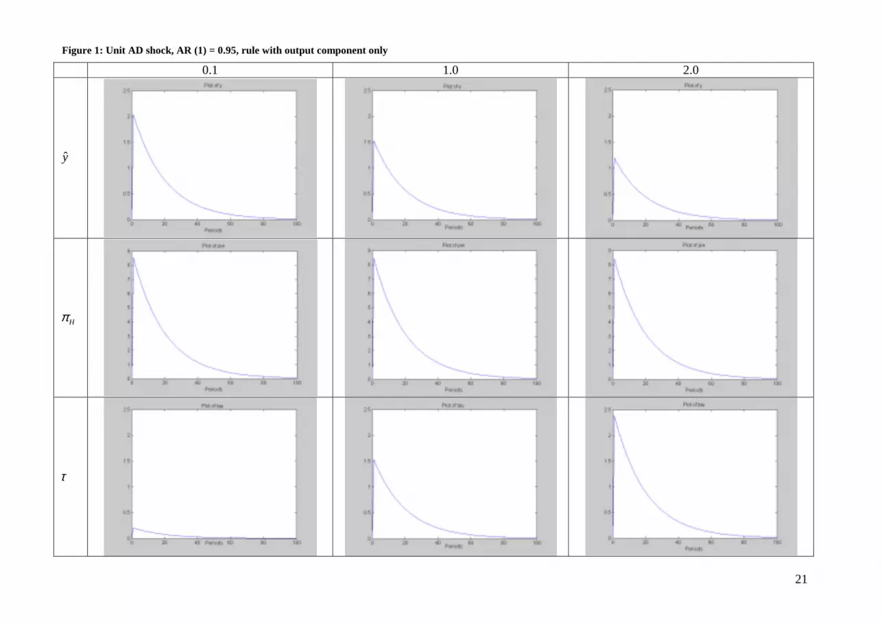
Figure 1 plots the reaction, under different sensitivities of taxation to the output gap, to a per-

sistent unit aggregate demand shock in period one. It shows that increasing consumer taxation

in response to the shock can actually reduce the deviation of output from its steady-state level.

It affects the size of the output gap. The time that it takes to return to equilibrium is not short-

ened, however. The impact on inflation is only marginal. The reason is that there are two op-

posite effects at work. Raising the tax rate dampens the output gap and thus reduces inflation-

ary pressure. But, on the other hand, the tax also reduces nominal wages and therefore enters

the Phillips curve (33) in a direct way. The main difference between fiscal and monetary pol-

icy is thus that the consumer tax affects aggregate demand and labour supply, whereas the lat-

ter is limited to the effect on aggregate demand.

*** Figure 1 ***

The reaction to the unit demand shock under a monetary policy rule, where the sensitivity of

the nominal interest rate to the output gap is taken as in the above taxation rule, is reported in

16

figure 2. The pictures reveal a somewhat stronger dampening effect on the output gap. Con-

trary to the tax rule, the increase in the interest rate also leads to a pronounced decline in infla-

tion. Finally, the implied variation of the policy instrument, the deviation of the nominal from

the equilibrium real interest rate, is lower than in the fiscal policy case. A potential advantage

of the variable VAT component however is that it does not face a zero lower-bound con-

straint.

*** Figure 2 ***

The next two figures display the impulse responses to the persistent unit aggregate supply or

cost-push shock. In this event, monetary policy faces a trade-off between output stabilization

and inflation. For fiscal policy this trade-off is less pronounced, however. One the one hand

side, lowering the consumer tax helps to narrow the output gap, whereas the resulting increase

in inflation, one the other hand, is rather small. Again, the reason is that the tax has two oppo-

site effects on price level changes. It enters the Phillips curve indirectly, via the output gap, as

well as directly, because it reduces the real wage.

*** Figure 3 ***

For monetary policy the output-inflation trade-off is obvious. Lowering interest rates, on the

one hand, narrows the output gap. The effect is stronger than in then fiscal policy case. But,

on the other hand, the increase in inflation following the cost-push shock becomes more pro-

nounced under an output-oriented policy rule. As for the demand shock above, the variation in

the policy instrument is stronger under the fiscal rule. Note, however, that with an output sen-

sitivity of monetary policy as high as in our example the zero lower-bound constraint may be

binding.

*** Figure 4 ***

A time varying component in consumer taxation may, in sum, contribute to smooth fluctua-

tions in output that are driven by persistent demand or cost shocks. The narrowing of the out-

17

put gap that can be achieved is somewhat smaller than for a monetary policy that operates

with an equivalent output sensitivity of interest rate choices. The variation of the tax compo-

nent thus needs to be stronger to achieve a similar degree of output stabilization. Inflation, on

the other hand, is almost insensitive to temporary changes in the VAT. Given an aggregate

demand shock, fiscal policy therefore fails to achieve the same amount of output and inflation

stabilization as monetary policy. In the event of a cost-push shock, on the other hand, the fis-

cal rule is less exposed to the trade-off between output and inflation stabilization.

5. Conclusions

The present paper investigated the potential of fiscal policy for macroeconomic stabilization.

To this aim, we modified the small open-economy specification of Clarida et al. (2001), and

Galí and Monacelli (1999) in order to include a time-varying tax rate on consumption. This

adjustable tax rate has then been taken as the fiscal policy tool.

We calibrated the model with what seem to be plausible parameter values for small euro area

countries. The simulation exercise then compared impulse responses for fiscal rules with dif-

ferent sensitivities to the output gap. To this aim, we have focused on the situations of persis-

tent aggregate demand and aggregate supply shocks. Impulse responses for monetary policy

under an interest rate rule with equivalent output sensitivity were presented in order to make

some informal comparison between the stabilizing potential of consumer tax and interest rate

variations.

The preliminary results suggest that time-varying consumer taxation may contribute to

smooth macroeconomic fluctuations. Nevertheless, the stabilizing potential of monetary pol-

icy with respect to output and inflation seems to outperform fiscal policy rule in the event of

persistent aggregate demand shocks. With adverse supply shocks, our fiscal policy rule how-

ever experiences less of a trade-off between output and inflation. In both scenarios, variations

in the fiscal policy tool need to be stronger to bring about an equivalent degree of output

stabilization than monetary policy.

From the perspective of stabilizing macroeconomic fluctuations, the variable VAT component

may thus be considered as an imperfect substitute for the loss of monetary policy at the na-

tional level. At this stage the result is only of tentative nature, however. The weaknesses and

potential merits of taxation-based stabilization shall be investigated further in subsequent

work. To this aim, a quantitative, loss-function based evaluation should be added. Further-

more, one should consider the case of large open economies in a monetary union, e.g. along

18

the lines of Beetsma and Jensen (2002, 2004). In addition, the analysis could also be extended

to direct taxation.

References:

Ballabriga, Fernando, Carlos Martinez-Mongay (2003): Has EMU shifted policy?, Economic

Papers 166, European Commission

Beetsma, Roel, and Henrik Jensen (2002): Monetary and fiscal policy interactions in a micro-

founded model of a monetary union, ECB working paper 166

Beetsma, Roel, and Henrik Jensen (2004): “Mark-up fluctuations and fiscal policy stabiliza-

tion in a monetary union”, Journal of Macroeconomics 66, 357-376

Blanchard, Olivier, and Charles Kahn (1980): “The Solution of Linear Difference Models un-

der Rational Expectations”, Econometrica 48, 1305-1311

Bofinger, Peter (2003): “The Stability and Growth Pact Neglects the Policy Mix between Fis-

cal and Monetary Policy”, Intereconomics 38 (1), 4-7

Bohn, Henning (1998): “The Behavior of U.S. Public Debt and Deficits”, Quarterly Journal of

Economics 113 (3), 950-963

Buti, Marco, and Paul Van den Noord (2003): What is the impact of tax and welfare reforms

on fiscal stabilizers? A simple model and an application to EMU, European Economy 187

Calmfors, Lars (2003): "Fiscal policy to stabilize the domestic economy in the EMU: What

can we learn from monetary policy?", CESifo Economic Studies 49 (3), 319-353

Clarida, Richard, Jordi Galí, and Mark Gertler (1999): “The science of monetary policy: A

New Keynesian perspective”, Journal of Economic Literature 37 (4), 1661-1707

Clarida, Richard, Jordi Galí, and Mark Gertler (2001): "Optimal monetary policy in open vs.

closed economies: An integrated approach", American Economic Review 91 (2), 248-252

Clarida, Richard, Jordi Galí, and Mark Gertler (2000): "Monetary policy rules and macroeco-

nomic stability: Evidence and some theory", Quarterly Journal of Economics 105 (1), 147-

180

European Commission (2003): European Economy - Statistical Annex, Bruxelles

Fagan, Gabriel, Jerome Henry, and Ricardo Mestre (2001): An area-wide model for the euro

area, ECB working paper 42

19

Galí, Jordi (2003): “New Perspectives on Monetary Policy, Inflation, and the Business Cy-

cle”, in: Mathias Dewatripont, Lars Hansen, and Stephen Turnovsky (eds.): Advances in

Economics and Econometrics, Vol. 3, Cambridge: Cambridge University Press, 151-197

Galí, Jordi, and Roberto Perotti (2003): "Fiscal policy and monetary integration in Europe",

Economic Policy 37 (3), 535-572

Galí, Jordi, and Tommaso Monacelli (2002): Monetary policy and exchange rate volatility in

a small open economy, NBER working paper 8905

Galí, Jordi, Mark Gertler, and David Lopez-Salido (2001): "European inflation dynamics",

European Economic Review 45, 1237-1270

Juillard, Michel (1999): “The Dynamic Analysis of Forward-Looking Models”, in: Andrew

Hughes Hallett and Peter McAdam (eds.): Analyses in Macroeconomic Modelling, Bos-

ton: Kluwer, 207-224

McCallum, Bennett, and Edward Nelson (1997): An optimizing IS-LM specification for

monetary policy and business cycle analysis, NBER working paper 5875

Mountford, Andrew, and Harald Uhlig (2002): What are the effects of fiscal policy shocks?,

CEPR discussion paper 3338

Perez, Javier, and Paul Hiebert (2002): Identifying endogenous fiscal policy rules for macro-

economic models, ECB working paper 156

Schmitt-Grohe, Stephanie, and Martín Uribe (2003): Optimal simple and implementable

monetary and fiscal rules, mimeo

Taylor, John (2001): "Reassessing discretionary fiscal policy", Journal of Economic Perspec-

tives 14 (3), 21-36

Taylor, John (1993): "Discretion versus policy rules in practice”, Carnegie-Rochester Confer-

ence Series on Public Policy 39, 195-214

Wijkander, Hans, and Werner Roeger (2002): "Fiscal policy in EMU: The stabilization as-

pect", in: Marco Buti, Juergen von Hagen, and Carlos Martinez-Mongay: The Behaviour

of Fiscal Authorities, Basingstoke, 149-166

Wyplosz, Charles (2001): Fiscal policy: Institutions and rules, mimeo

20

Annex:

Impulse responses in the unregulated system

Unit AD shock, AR (1) = 0.95 Unit AS shock, AR (1) = 0.95

y

Hπ

21

Figure 1: Unit AD shock, AR (1) = 0.95, rule with output component only

0.1 1.0 2.0

y

Hπ

τ

22

Figure 2: Unit AD shock, AR (1) = 0.95, interest rate rule with output component only

0.1 1.0 2.0

y

Hπ

ri −

23

Figure 3: Unit AS shock, AR (1) = 0.95, rule with output component only

0.1 1.0 2.0

y

Hπ

τ

24

Figure 4: Unit AS shock, AR (1) = 0.95, interest rate rule with output component only

0.1 1.0 2.0

y

Hπ

ri −