COOLBAUGH, DYLAN T., M.A. Evaluating the Potential Locations for Transit-Oriented Development (TOD): A Case Study of Mecklenburg County, NC. (2016) Directed by Dr. Selima Sultana. 91 pp.

The work described is aimed at developing a unique and modifiable model for

analyzing transit system improvements, with specific emphasis on the concept of Transit-

Oriented Development (TOD). In particular, the use of multiple variables that have been

developed over the years as a result of a number of transit analyses, in a novel manner is

described. The area of study was the light rail transit system (LRT) known as Lynx in

Mecklenburg County, NC and over a period of development between 2001 and 2012

which included the actual construction phase from 2005 to 2007. An index model was

developed to combine and magnify the potential impacts of each of the identified

variables as they related to one another and the surrounding urban environment. These

variables included land value, housing unit density, and others that are often been

associated with TOD. The results of this combined and comprehensive analysis served to

identify areas that are likely associated with the transit system, primarily proximity to the

LRT system, i.e., areas where changes in the TOD-related variables were consistent with

a positive relation to recognized TOD principles. Some areas within the service area

showed especially high positive attributes of TOD, for example, Uptown Charlotte, a

major hub of a current phase of LRT development, as well areas of other future

enhancements. An extension of the work described should include the evaluation of

additional variables as applicable data sets are made available, including, but not limited

to, employment change, property vacancy statistics, and crime.

 

  

EVALUATING THE POTENTIAL LOCATIONS FOR TRANSIT-ORIENTED

DEVELOPMENT (TOD): A CASE STUDY OF

MECKLENBURG COUNTY, NC

by

Dylan T. Coolbaugh

A Thesis Submitted to the Faculty of The Graduate School at

The University of North Carolina at Greensboro in Partial Fulfillment

of the Requirements for the Degree Master of Arts

Greensboro 2016

Approved by  

_______________________________ Committee Chair

 

  

© 2016 Dylan T. Coolbaugh

 

ii  

APPROVAL PAGE

This thesis written by DYLAN T. COOLBAUGH has been approved by the

following committee of the Faculty of The Graduate School at the University of North

Carolina at Greensboro.

Committee Chair _____________________________________

Committee Members ________________________________________

_______________________________________

March 22, 2016______________ Date of Acceptance by Committee May 27, 2015______________ Date of Final Oral Examination

 

iii  

ACKNOWLEDGEMENTS

This thesis would not have been possible without the guidance and the help of

many individuals who contributed much of their valuable time to assist in the completion

of this study. I would first and foremost like to thank my supervisor and committee chair,

Dr. Selima Sultana, who guidance, experience and knowledge challenged and enriched

my understanding for all steps to completing this work.

I would also like to thank Dr. Keith Debbage and Dr. Zhi-Jun Liu for their

encouragement and guidance as committee members and professors.

This research could never have been completed without data provided by Scott Black at

City of Charlotte-Mecklenburg County GIS, from whom I received data at the tax parcel

level for 12 years which allowed for a spatio-temporal approach to transportation

analysis.

Finally, I would like to thank my family and fiancée for all of their help, support

and attempts to understand what I was talking about throughout this entire process. I am

here because of all of their love and support.

 

iv  

TABLE OF CONTENTS

Page

LIST OF FIGURES ........................................................................................................... vi

CHAPTER

I. INTRODUCTION .................................................................................................1

1.1 Background and Research Questions.....................................................1

II. LITERATURE REVIEW .......................................................................................7 2.1 Transit Oriented Development: A Brief Background ............................7 2.2 Studies of Charlotte Light Rail ............................................................10 2.3 Transit and Land Use Relationships and Implications ........................12 2.4 Value Capture as a Means to Pay for Transit ......................................15 2.5 Ability for High Speed Rail to Capitalize on Abandoned Rail ............18 2.6 Assessments of Large Scale Transit Improvements ............................19 2.7 Effect of Mass Transit on Land and Property Values ..........................20 2.8 Bicycle Transit Analysis ......................................................................24

III. RESEARCH DESIGN .........................................................................................26 3.1 Study Area ...........................................................................................26 3.2 Time Frame, Data Sources and Methodology .....................................30 3.3 Variable Weights Explained ................................................................34 3.4 Methodology ........................................................................................35

3.4.1 Change in Land Value ..........................................................37 3.4.2 Change in Housing Style and Land Uses ..............................39 3.4.3 Bus Transit Station Density ..................................................40 3.4.4 Population Change from 2000 to 2010 .................................42 3.4.5 Transit Station Accessibility in Mecklenburg County ..........45

IV. RESULTS AND ANALYSIS ..............................................................................47 4.1 Evaluation of Benefits from Transit Development in

Mecklenburg County .......................................................................47 4.1.1 Change in Land Value ..........................................................47 4.1.2 Changes in Housing Unit Density.........................................52 4.1.3 Bus Station Analysis .............................................................55 4.1.4 Population Change ................................................................56

 

v  

4.1.5 Accessibility Analysis ...........................................................59 4.2 Development of Index Model for Transit-Oriented

Development ...................................................................................61 4.2.1 The Value of Raster Conversion ...........................................63

4.3 Existing TOD in Charlotte ...................................................................64 4.4 Index Value Interpretations ..................................................................67

4.4.1 Emerging Transit-Oriented Development .............................68 4.5 Assessment of Demographic Changes, Vehicle Ownership and Mode Split ........................................................................................69

4.5.1 Changes in Characteristics for Census Block Groups near Existing Rail Stations ..............................................69

4.5.2 Changes in Characteristics for Census Block Groups near Planned LRT Stations .............................................71

4.5.3 Changes in Characteristics for Census Block Groups not near Planned LRT Stations .......................................72

4.6 Employment and Job Growth in Mecklenburg County .......................73  

V. CONCLUSIONS ..................................................................................................75 5.1 Conclusions and Discussion ................................................................75 5.2 Pre-Existing Limitations ......................................................................76 5.3 Future Directions .................................................................................77

REFERENCES ..................................................................................................................79

 

vi  

LIST OF FIGURES

Page

Figure 3.1. Mecklenburg County, North Carolina Study Area ..........................................28

Figure 3.2. Ridership on the Lynx, 2008-2014 .................................................................29

Figure 3.3. Visualization of Raster Layers and their Combination ..................................34

Figure 4.1. Land Value Changes from 2001-2012 ...........................................................49

Figure 4.2. Analysis of Total Land Value Change, 2002-2012 ........................................51

Figure 4.3. Changes in Housing Units, 2001-2012 ...........................................................53

Figure 4.4. Assessment of Change in Housing Unit Density, 2001-2012 ........................54

Figure 4.5. Analysis of Bus Density in Mecklenburg County ..........................................55

Figure 4.6. Population Change Characteristics .................................................................58

Figure 4.7. Analysis of Population Change, 2000-2010 ...................................................59

Figure 4.8. Assessment of Accessibility in Mecklenburg County ....................................61

Figure 4.9. Final Calculation of TOD in Mecklenburg County ........................................66

Figure 4.10. Vehicle Usage Numbers near Existing Stations, 2000-2010 ........................71

Figure 4.11. Usage Numbers near Planned Stations, 2000-2010 ......................................72

Figure 4.12. Usage Numbers not near Stations, 2000-2010 .............................................73

Figure 4.13. Growth between Charlotte and Mecklenburg, 2005-2012 ...........................74

Figure 5.1. Future Development Plans of the Lynx Transit System .................................78

 

1  

CHAPTER I

INTRODUCTION

1.1 Background and Research Questions

In recent decades there has been an increased interest in exploring the value

associated with developing or expanding quality public transportation within several U.S.

cities. This is not surprising since it would appear to be the case that numerous urban

environments would benefit from enhanced public transit systems and any associated

transit-oriented development (TOD) that would result, i.e., development that may be

attributed directly to the existence of a public transit system generally due to proximity.

However, there is a negative perception that building or expanding public transit systems

will only provide benefit to the relatively few people who would actually use them, and

that the high costs incurred during construction and system operation will outweigh any

such benefits. As a result, some feel that significant investment in mass transit may not

be a viable option for most American cities (Littman, 2014). Perhaps because of this, the

United States lags well behind other countries that have taken the initiative in recent

years to boost public transportation on a national scale, e.g., countries such as China,

South Korea, and the UK. As a further challenge to investing in new transit systems, it

appears that in the US investment to maintain the existing infrastructure is often

inadequate (Novak, et al., 2012).

 

2  

In recognition of the scarcity of thorough analyses of transit system projects and

the potential value that could be associated with TOD, the focus of this thesis is to

evaluate the costs and expected service lifetime benefits associated with the development

of a public transit project by examining the light rail project (Lynx) in Mecklenburg

County, North Carolina, as a case study. The primary goal of this research is to develop a

model that considers a cost/benefit analysis for use in this and other scenarios. This

model could then be utilized by researchers to better predict potential benefits with

varying urban infrastructure changes before construction begins (see for example:

Topalovic, et al., 2012, Smith and Gihring, 2006, Baum-Snow, et al., 2005). The

questions for the described research are based on an apparent lack of comprehensive

modeling research and assessments for determining total benefits of large scale public

transit improvements (Baumel, et al., 1977, Cervero, 2003, Novak, et al., 2012 and others

listed in Section II below).

For reference, there have been research efforts focused on a variety of

development activities that relate to city and county-wide changes. However, there have

been relatively few studies aimed at assessing the impacts that new and improved

transportation systems have on the surrounding urban framework from a complete and

comprehensive perspective. Two of the most notable areas of study have been New York

and Washington states. For example, two major studies were performed that identified

key infrastructure investments in Seattle, ranging from highway development during the

1950’s to more recent planning for a public transit network (Batt, 2001 and Gihring,

2001). In general, though, assessments have been primarily theoretical and usually

 

3  

performed after project completion, thereby having the benefit of 20/20 hindsight and not

relying on the development techniques for current and future site-predictive analyses.

Public transit can create various types of impacts, both positive and negative, and

a more comprehensive evaluation should consider all significant factors, an approach that

is not usually considered. High quality public transit can stimulate TOD in compact,

multi-modal neighborhoods where residents tend to own fewer vehicles, drive less and

rely more on alternative modes than in more automobile-oriented communities. This can

leverage additional travel reductions and regional benefits beyond that of just the travel

from a private to public mode. For example, the construction of a transit system may

lead to appreciation in residential property values which could lead to further investment

in a specific locale (Kay et al., 2014). The potential for a synergistic relationship between

one type of development and another could lead to enhanced urban environments and it is

important to understand these relationships, although it is not likely to be a simple

evaluation since it encompasses a vital ecosystem of a broad spectrum of people and the

places in which they work and live. Every change within a business or neighborhood

community, whether it is additive or destructive, will have differing degrees of

consequences. In this context, the immediate or long term aspects associated with new

transit projects should be researched, tested and modeled to determine and better

understand their efficacy, level of impact, and ultimately, their potential for lasting value.

While no model has attempted comprehensive examinations of city (or county)-

wide public infrastructure, some recent studies have worked to develop models for new

additions to the urban environment. For example, bike share systems have been

 

4  

developed in recent years in cities such as Seattle, WA, Washington, D.C., and

Minneapolis, MN (University of Washington Bike-Share Studio 2010, Maurer 2011) and

serve as good examples of what can be done with respect to the beginning of a more

comprehensive study approach. In particular, these studies have taken successful

geographical information system (GIS) approaches to a comprehensive assessment of key

factors relative to bike share use, e.g., popularity, and financial success, and used them to

develop unique and novel models for identification of prime locations where bike share

stations would be utilized most efficiently. However, these models apply to a single

mode of transit with very specific ridership characteristics and examine highly focused

results, for example, travel lane needs, impacts on property and land values. To be more

effective, models should be able to be modified and adjusted to apply to different scales

and levels of impact.

A key factor considered in this thesis is the relationship between the presence of

TOD and a positive correlation between public transit use and indicators of cultural or

socioeconomic value growth. For example, in areas of a city where public transportation

exists and is used regularly by residents and commuters, one would expect to see multi-

family housing (e.g., apartment complexes) and conglomerations of businesses, both

public and private, i.e., an indication of a healthy community. In such a community, the

properties closest to the transit system would likely possess higher land and these would

increase with decreasing distance to a transit station. Other factors will be identified and

examined as well with the goal of extending beyond previously completed studies.

 

5  

In general, the purpose of much of the past work has been to develop a suitable

methodology for the analysis of public transportation systems. Since it is desirable to be

able to apply the model to the broadest range of cases, it would be advantageous to have a

more generalizable model. Past research has examined bus systems, rapid transit and

light rail transit, and the manner in which demographic and census data have been used to

perform cross-sectional analyses and to better understand any regional impacts that were

reported (Novak, et al., 2012; Perry and Babitsky, 1986; Smith, 1987; Parry and Small,

2009). Based on these past efforts, it appears that key factors that are important in order

to improve upon the previous research, and in an effort to avoid reinventing the wheel,

are land values and housing units assessed from tax parcel and property data, population

change data gleaned from the 2000 and 2010 census results, and current bus stop and

LRT route information. By focusing on these inputs, it should be possible to develop an

index model that can perform a superior analysis that will provide insight into how

proposed projects to improve transit systems may affect adjacent urban environments,

both positively and negatively.

In keeping with the discussion above, the objectives of this thesis are:

1) To examine the attributes and variables associated with Transit-Oriented

Development (TOD) with particular emphasis on Mecklenburg County, North

Carolina.

2) The development of an index model for TOD based on Mecklenburg County’s

Lynx light rail transit (LRT) system.

 

6  

3) The determination of locations of existing TOD and possible locations of

emerging TOD in the context of the planned extension of the Lynx LRT system.

4) Verification of the model by examination of changes in demographic

characteristics and mode choices through the use of specific census data.

5) A discussion of potential future research that may be undertaken with respect to

applying the model in order to better understand future regional trends, e.g.,

employment, housing, business development, transit needs/opportunities.

 

7  

CHAPTER II

LITERATURE REVIEW

2.1 Transit Oriented Development: A Brief Background

As mentioned above, transit-oriented development (TOD) revolves around the

relationships between public transit systems and the urban environments in which they

exist. In other words, it examines the manner in which people, places and things interact

with public transit and vice-versa.

There are several studies that have gone to great length to discuss what TOD is

and how to measure it (Cervero and Landis, 1996; Gihring, 2001; Dorsey and Mulder;

2013; Kay, et al., 2014). In general, the consensus is that TOD entails the existence of

certain characteristics within proximity to public transit improvements that correlate the

usage of lifestyle-relevant characteristics to the growth of public transit. Such

characteristics include proximal location of multi-family housing, spacing between

individual transit stops, accessibility and connectivity of sidewalks or bike lanes to transit

stops, and positive potential of land value growth.

Although TOD in its most basic form has existed for millennia (Carlton, 2007),

the true conceptualization of TOD as “a neo-traditional guide to sustainable community

design” has only been observed more recently (Calthorpe, 1993). As Carlton (2007)

describes the general form of TOD, it consists of mixed-use communities that serve to

encourage people to live near transit services and decrease their dependence on driving.

 

8  

With the emergence of light rail and streetcars as primary modes of public transit in the

1970’s and 1980’s, there also emerged some opportunities for developers and

governments to capitalize on the developing transit areas as dense urban nodes.

Residents could live and work nearby one another, utilize public transit for commuting

and personal trips, and governments could capitalize on the opportunity to reduce urban

and rural sprawl. In theory, the idea was very progressive and had the potential to create

a new paradigm of growth. In practice, though, TOD was found to be demonstrable in

only a few places, primarily due to a lack of understanding and outdated planning

strategies.

TOD may apply to both public (bus, light rail) and private transit modes (personal

vehicles), although the idealized concept revolves around public modes only. In the

context of private transit, TOD can be identified in the 1950’s with the advent of the

automobile and highway boom. Many off-ramp locations adjacent to highways gained

considerable growth in jobs and land value. Even in areas where private landowners

withheld land, their properties gained considerable increases in value simply due to the

properties’ proximity to transit nodes. TOD has been shown to have direct relationships

to growth in land value and the potential for value capture through post-system

development analyses (Batt, 2001; Gihring, 2001).

Urban locations such as Seattle, WA and Portland, OR actively embraced the idea

of public transit long before TOD was popularized. As an example, the city of Portland

deviated from the norm of the late 1950’s concept of building massive highway systems

and instead focused on internal transportation, developing complex bus networks and

 

9  

incorporating light rail and streetcar systems. TOD emerged in Portland due to their

forethought and comprehensive plans. Many other locations attempted similar strategies,

but the attempts may have been too late to make a difference with any pre-existing

conditions, and the level of understanding and planning skills at the time.

For instance, the San Francisco Bay Area developed and installed the Bay Area

Rapid Transit system (BART) in the 1970s. Cervero and Landis (1996) looked at how

the system had interacted with the surrounding urban framework during its 25 year

lifespan. Prior to this study, a few others had also tried to characterize the success or

failure of the system as a TOD (Merewitz, 1972; Webber, 1972; Knight and Trygg, 1977;

Johnston and Tracy, 1983). Those studies had determined that areas proximal to BART

stations had developed less job and value growth over the years than had other areas,

deeming the system a failure. A potential problem with those studies was that they

focused on percentages of job change proximal to transit stations against total job change

in the region to measure the effectiveness, instead of considering the actual numbers.

When Cervero and Landis (1996) looked at the differences in job and value growth in

actual numbers, they were far higher in BART-served areas than others. Under these

circumstances, the system was deemed to be a mostly successful example of TOD.

The caveat in the Cervero and Landis (1996) study was that the locality of the

majority of job and value growth resided mostly in San Francisco itself and only a small

portion of growth occurred in areas along the BART system outside of San Francisco. As

a result, the overall BART system was observed to have some area-specific TOD

successes, but it was not the complete success that it might have been with a more

 

10  

complete understanding of the greater Bay Area transit needs. In theory, for TOD to be

successful, there should be growth throughout, although it does not have to be equally

distributed.

In the instance of Seattle, the regional government and citizens passed legislation

that placed a partial tax on properties that gained increases in land value directly

attributable to proximity to public transit nodes. Gihring (2001) looked at how the region

went about achieving this end, and how it benefitted public transit and the people of

Seattle. A primary conclusion was that site value increased independently of building

improvements. These site value increases, according to economic theory, should reside

legitimately with the creator of the value, i.e., value that can be directly attributed to

proximity to transit improvements should be returned to the system. Such examples are

necessary when talking about TOD and how it actually works, although there are still far

too few examples in the United States. Using existing situations where TOD has worked

is necessary for developing new plans and methods for utilizing existing spaces to

achieve similar results.

2.2 Studies of Charlotte Light Rail

Studies of specific light rail systems are difficult to find, since LRTs are

developed relatively infrequently. The only study available that assessed spatio-temporal

characteristics was done by Yan et al. (2012), in which they studied the Charlotte Lynx

LRT, focusing on how the inclusion of a new LRT system impacted single-family

property values. The primary method of analysis that was chosen for the system

consisted of a hedonic price analysis (HPA) since it could incorporate the regression

 

11  

analyses performed on the four phases of development: pre-planning, planning,

construction and operation. In general, the hedonic approach assesses the value of an

ecosystem or a set of environmental services based on its characteristics and is often used

in attempts to value housing markets. The overall time period for the study was 1997 to

2008 using data that contained sales price information for single-family houses within a

network distance of 1.6 km.

The variable that Yan et al. (2012) considered to be most important for the

independent variables was the analysis of station distance which was calculated as the

logarithm of the network distance from a parcel to its nearest transit station. Using this

method of assessment took into account the long understood principle of distance decay

whereby the influences of the transit station decreases at an exponential rate the farther

that properties are located from a given station, i.e., the ecosystem service. Network

distance was chosen instead of Euclidean distance, as it gives a real world representation

of how a resident is expected to navigate to the destination from the origin.

An important conclusion from this study was that distance to a rail station had varying

influence depending on which phase was regressed. For the second and third phases,

1999-2005 and 2005-2007, respectively, the coefficient for the logarithmic network

distance variable indicated that housing prices were generally higher the farther away

from stations they were. It was suggested that this was largely due to the fact that the

Lynx rail line was originally a freight rail line and a large proportion of adjacent

properties were dedicated to industrial uses, something that had diminished housing

 

12  

values nearby. This relationship appeared to have a negative effect on surrounding

values, however, by the fourth phase the negative influence appeared to have dissipated.

The primary conclusion of the researchers was that for the first three phases of the scope

of the study, proximity to future rail stations had a negative impact on surrounding

housing prices. An explanation for this initial negative relationship was likely due to the

presence of adjacent industrial uses that often are not compatible with single-family

housing. After the system began operation, housing prices began to react positively to

proximity to stations. It is likely that improved access to reliable transportation served to

improve the attractiveness of living nearer to transit stations, or that unattractive

industrial land uses had been relocated away from the Lynx line.

Additionally, the researchers mention some of the limitations of their datasets,

including a lack of access to tax parcel files with land value fields, a much more useful

variable for physical relationships. Also, they mentioned that a lack of data for more

years after the system came into operation was a hindering factor.

2.3 Transit and Land Use Relationships and Implications

There have been some significant strides in research with regards to linking public

transportation and land uses. For example, Cervero and Landis (1996) assessed the Bay

Area Rapid Transit (BART) system in San Francisco to determine the direct and indirect

impacts the system had on land use and development over a twenty five year period of its

operation. The hope of planners, in creating a modern era rail system, was to guide

future population and employment growth in the region. As mentioned previously,

BART was expected to strengthen the Bay Area’s urban centers, while guiding suburban

 

13  

growth along radial corridors (hub and spoke) in the post WWII-era with that expectation

that it would ultimately lead to a star-shaped, multi-centered metropolitan form. The

theory in this development pattern was that building on the periphery and having

uncoordinated land development imposes added costs on land owners, which could be

avoided by having a firm plan and a desire for compact development. Incentive zoning

had a big impact on land use and TOD around stations.

Unfortunately, some studies performed on the region found, or at least claimed,

that BART most likely redistributed growth that would have occurred anyway, albeit in a

more dense fashion. These studies were in line with much of the criticism of BART,

stating that the potential usefulness of the system was hampered by “too little, too late.”

The major highways in San Francisco had been established for years before the BART

system had begun development, with much of the peripheral and costly low density

development having been already underway.

On the other hand, demographic data paint a different picture. Cervero and

Landis (1996) argue that BART-served, “super-districts” drew over 140,000 more

residents than non-BART-served, “super-districts.” The previously mentioned studies

relied heavily on straight percentages, which reversed the results. 153,000 more jobs

were created in BART-served regions during the time period from 1970 to 1990. After

disaggregating the data to the zip code level, the team found that job growth was higher

in BART-served areas, consistent with the “super-district” level data analysis. The

results were underscored by the fact that most of the growth occurred in downtown San

Francisco. Broken down further, the job analysis at the zip code level also revealed that

 

14  

FIRE jobs (financial, insurance and real estate) benefitted from the most growth, over

108% for the time period, non-business showed growth of almost 53%, and business

showed a growth of over 46 %. Cervero and Landis (1996) concluded that BART may

have been responsible for slowing job decentralization from downtown San Francisco

and that BART stations were positively correlated with high population and employment

densities in the Bay Area generally, and San Francisco specifically.

Cervero (2003) considered the idea of smart urban growth with a focus on

California, and more specifically at the Los Angeles and San Francisco areas. He

contends that transportation problems in California are a direct extension of housing and

land-use problems, with sprawl and lack of affordable housing topping the list. Other

land-use related problems are the housing market distortions and non-fiscally responsible

land use decisions. Cervero (2003) began by pointing out the vast needs of California as

far as lack of mobility, tremendous congestion, and excessively long travel times for

many residents, as affordable living exists far from most employment centers. He

provided significant examples that demonstrate both failings and successes across the

state.

Giuliano (1988) focused on Milwaukee and looked at residential and firm

locations as they relate to work force and agglomeration economies. Agglomeration was

measured as the sector’s share of total employment within each municipality, with the

labor force defined as the measured number of workers in the sector located within a

radius of the municipality as well. A regression was performed on the six industrial

sectors, with distance from the Milwaukee central business district being positively

 

15  

related to location choice, perhaps related to demand for cheaper land within the suburbs.

It was also pointed out that an earlier study (Herzog, et al., 1986) identified factors

influencing location choices for high technology workers. Other than a higher degree of

mobility, choices for these workers were not dissimilar to those of other workers.

Additional factors were identified, including labor force characteristics, transportation for

workers, and proximity to local activity centers. Simpson (1987) determined that both

workplace and residential locations needed to be looked at simultaneously because they

are functions of each other, although residential location was found to exhibit a greater

overall influence on workplace location.

Giuliano (1988) suggests some means of revising existing theory, by including a

temporal element to create dynamic models that display multi-faceted changes over time,

primarily to allow for comprehensive cost-benefit analyses. Also, it was suggested that

the total household commute cost over the housing tenure should be considered as a

means of assessing transport costs, since households may use this to optimize access to

possible employment opportunities over the relevant total time period. One conclusion

was that labor force was the most important factor with respect to firm location, and that

once a relocation site was established, growth followed.

2.4 Value Capture as a Means to Pay for Transit

Value capture is a category of methods for recouping costs of public infrastructure

improvements wherein residents and local businesses that directly benefit from the

improvement, through vast land value increases, more business revenue, etc., pay a

percentage of that direct benefit attributed to adjacency to the improvement back to the

 

16  

system itself. Methods include a land value tax and a publicly-approved sales tax

increase. The land value and sales tax approaches are most important because they have

been theorized and modeled the most (e.g., land value tax or land capital gains tax) and

actually applied to public infrastructure investment, for example, a half-cent sales tax

increase. Another method that has been utilized in the U.S. to a lesser extent is the

leasing of air rights, which has had significant success in Seoul, South Korea, in

conjunction with high levels of transparency and cooperation between public and private

interests (Cervero, 2009).

Two researchers that have provided strong evidence in recent years that value

capture should be utilized for major public transit projects are Batt (2001) and Gihring

(2001). Batt focused on a major highway improvement in New York from the 1950’s,

the Northway, where private landowners benefitted significantly from adjacency to the

improvement with collective land values increases within 3.25 km of the Northway of

over $3.7 billion. Gihring (2001) focused on the Seattle region, where public

improvement projects surpassed expectations and private residents and business owners

enjoyed a bloom in personal land valuation. Gihring (2001) primarily aimed his research

at how regions can build support for value capture and the utilization of TOD practices.

Similarly, other research has also provided significant contributions to value

capture theory and analysis (Cervero, 2009; Smit and Trigeorgis, 2009). As an example,

Cervero (2009) looked at San Francisco, Seoul, South Korea and Hong Kong, China to

assess how replacement of elevated freeways with greenways, boulevards and advanced

public transit systems could serve to boost local communities and land values. He

 

17  

provided evidence indicating the importance of assessing infrastructure and its

relationship with surrounding urban areas. Some of the examples used include that of the

current president of Seoul (as of 2009) when he worked previously on developing and

initiating plans to remove the Cheong Gye elevated freeway. A primary goal was to

reveal a stream buried beneath the freeway and the construction of a park and bike path

along its entire length. In San Francisco, Cervero (2009) investigated office and retail job

and housing growth after the elevated Embarcadero Freeway was demolished in 1990 and

found that between 1990 and 2000 growth was considerably faster than in previously

recorded periods. Hong Kong has a strong example of successful value capture policy

and practice as well. Their Mass Transit Railway Corporation (MTRC) has a rail and

property program that took a strong stance to maintain a healthy profit margin and played

an important “city-shaping role,” with each sector bringing specific natural advantages to

the railway corridor and creating successful TOD (Cervero, 2009).

Smit and Trigeorgis (2009) used a game theory approach to managing and valuing

assets in the existing market. The specific approach used in the valuation, Value of

Enterprise, took into account relationships between the value of existing assets, potential

growth value, flexibility of assets, and level of commitment from public and private

interests. The game consisted of analyzing how decisions can be influenced by a choice

to wait until conditions are more favorable and ideal, or build upon existing, continuously

changing conditions that may only serve to create temporary benefits. The method of

analysis was to use matrix evaluation of an example with two airports where both airports

choose to wait to expand, one or the other preempts growth or both airports choose to

 

18  

expand. Values are defined in the functions to correspond with the Nash equilibrium, a

concept in game theory that revolves around two or more non-cooperative players.

Results concluded that assessing the right time to build or invest in property, business, or

other assets around the infrastructure investment was a key factor in any scenario. The

same findings apply to growth strategies where the time from decision making to policy

implementation to completion could take decades and the use of a reliable model is

pivotal for establishing strategies and long term growth plans.

2.5 Ability for High Speed Rail to Capitalize on Abandoned Rail

To provide the greatest value to a particular region, legislators should focus their

efforts on assessing impacts at a level that transcends arbitrary boundaries since regional

scale improvements may possess synergies that more localized efforts most likely will

not. Much of the needed infrastructure already exists to develop and implement regional

high speed rail since, to a large degree, 18 wheeler trucking has replaced much of the

freight carrying that had once been transported by heavy rail, especially on the East Coast

of the United States. Upgrades could be completed at significantly lower costs, and bring

use to rail lines and return a much higher investment return than would otherwise result

from rusting or salvaged assets.

A study by Baumel, et al. (1977) attempted to assess the viability of upgrading

more than seventy rail lines in Iowa that are underperforming, in poor condition, or both.

The purposes of upgrading the rail would be to allow for higher load bearing rail cars

and to meet Federal Railway Administration (FRA) Class-II standards, which require

meeting certain speed conditions, e.g., a limit of 25 mph for freight rail and 30 mph for

 

19  

passenger rail, and having revenues greater than $9.34 million and less than $108.184

million for at least three consecutive years, in 1977 dollars. In terms of the evaluation,

mostly freight was expected to transit on the railways, but Baumel, et al., (1977),

included passenger movement as well in their calculations.

Ravibabu (2006) performed simple assessments and cost analyses for large scale

investments to determine whether Mumbai, India’s draft national urban transport policy

was correct in determining that surface rail was better off for suburban and fringe areas.

The cost of surface rail was compared to that of elevated rail and monorail, with the

conclusion being that upgrading existing surface rail would have a price tag that was 5%

that of elevated rail. Monorail was excluded because it was determined not to be feasible

for a ring rail network around the city and would only be useful for short distances and

minor passenger transit (Ravibabu, 2006).

2.6 Assessments of Large Scale Transit Improvements

Novak, et al. (2012), considered using the procedure of the scoping-based method

utilized by Vermont’s Transportation Project Planning Process. Vermont assesses

projects based on financial feasibility, safety issues, land use impacts, socio-economic

impacts, political and taxpayer concerns, and environmental impacts. Each of the asset

classes mentioned previously is used to prioritize each project and determine funding

allocations and priorities. In general, the conclusions were that Network Robustness

Index (NRI) values for the various projects varied considerably, from 4% decreases of

NRI all the way to 184% increases. Network Robustness Index (NRI) (Scott, et al.,

2006) is an evaluation of the change in total vehicle hours of travel (VHT) on the

 

20  

transportation network resulting from removal of one individual road link, not dissimilar

from the Cook’s D method of understanding the relative influence of individual records

during regression analysis. The highest value project, i.e., the one prioritized as the

project that should be approved and completed first, was a main street extension to Route

116, a high volume route that was determined to benefit from a more direct connection.

Surprisingly, few projects in post-assessment displayed any increases in NRI, which

would have indicated higher Vehicle Hours Travelled (VHT) on a system-wide scale. As

a result, a number of projects should have thus been prioritized at much lower levels.

This type of result, where increasing capacity of roadways may not lead to improvements

to congestion and travel times, has been denoted as Braess’ Paradox in which individual

users tend to choose to minimize personal costs of travel when faced with increased

capacity conditions,, unaware of the impact on other travelers (Pas and Principio, 1997).

Overall, the model did provide a means for Vermont to prioritize projects based

on their expected impact at a regional scale, and give projects with lesser impacts lower

priority or remove them altogether from the state budget. However, the outcomes were

not always as expected and this lends credence to the need for more advanced approaches

to allocate resources at all levels of government when determining how best to move

forward with maintenance and improvement of public transit systems.

2.7 Effect of Mass Transit on Land and Property Values

One of the primary considerations of this thesis is that mass transit affects a

number of indirect influences on the surrounding urban framework. Of primary

importance to businesses, home owners, and land owners is the concept that mass transit

 

21  

improvements can and will positively influence land and property values. However,

research into these effects, as well as existing empirical evidence to support the theories,

is somewhat limited. Some of the earlier work tried to conceptualize and define additions

to property values, the manner in which residents could take advantage, or were already

taking advantage of, the proximity benefits. Goldberg (1970) looked at relationships

between transportation, land values and rents, in addition to how demand affected each of

these variables. He found that as one lives further from the central business district

(CBD), land value increased dramatically in Vancouver from 1954 to 1968, but

accessibility dropped off. K.C. Koutsopoulos (1977) conceptualized the impact of mass

transit on property values as “reduction in travel costs (travel savings) afforded by a new

transportation alternative.”

Goldberg (1970) built upon past work, beginning with Haig’s (1926) study that

looked at the relationships between transportation and urban land values, focusing on

general transportation improvements while keeping all other things constant.

Considering the data available during that time period, and the computational

capabilities, that methodology was workable. Haig’s (1926) premise was that a general

transportation improvement will tend to lower aggregate rents when evaluating the

interconnectedness of site rents and transportation costs from a friction perspective since

there will be a greater ease of transit from locations farther away. In this sense,

transportation improvements were meant to overcome or reduce the friction that

prevented the public from moving from one location to another. Creating improvements

to the existing transit system should yield reductions in aggregate site rentals that would

 

22  

be dependent on the extent of the area under consideration and the centroids of

population density. His concept was fairly simple and it was expected that as activities

locate closer to the urban center, site rents increase and transportation costs decline. For

locations farther from the center, the reverse should be true.

Haig summed up these perspectives very well, “Of two cities, otherwise alike, the

better planned, from the economic point of view, is the one in which the costs of frictions

are lower.” One important criticism of the previously mentioned theories was that they

failed to take into account the size of the properties, considering the locations to be

points, rather than areas of differing size. This exclusion led to the theories falsely

developing models of high density around the city center. William Alonso pointed out

this concern and attempted to rectify it in his book, Location and Land Use: Toward a

General Theory of Land Rent. Goldberg developed a model to incorporate all three of the

variables of land rent, transportation cost, and site size, while considering time and

distance. He created a simple model of accessibility, relating activities to distance, along

with weights assigned to each “ring of accessibility.” Goldberg (1970) concluded that

transportation improvements that open up more urban land and raw materials will lead to

cheaper houses, dependent on the cost of construction which was found to be somewhat

analogous between small and large companies. Looking back at Haig’s arguments,

widespread growth away from the city leads to lower land values in the CBD, indicative

of competition within the region, as well as declines in rent values.

The accepted view of the role of transportation is to strongly affect social activity,

which warrants design to achieve social objectives. As a result, the policy value of

 

23  

transportation lies in the effects it can create. Much of the obstacles pertaining to public

transport investment and achieving the social goals intended, revolve around a lack of

quantitative information of the non-user and indirect impacts. According to

Koutsopoulos (1977), the work of Cribbens, et al., and Mohring attempted to rectify this

by looking at the impact of a transportation improvement as both a change in a

continuous phenomenon (accessibility) and a capitalization on travel savings afforded by

the improvement itself. Additionally, Mohring suggested that travel time savings would

be proportional to the distance from the improvement and the distance from the CBD.

Koutsopoulos performed regression analyses on old and new bus routes in

Denver, CO using multiple coefficients. The analyses showed that the variable

measuring impact of the bus routes on property values was statistically significant for

only four routes, all of which were bus routes in newer neighborhoods. Differences

between the old and new routes were most likely explained by “non-accessibility”

variables, represented by neighborhood and structural characteristics in the data.

Koutsopoulos suggested that the effect of neighborhood quality could provide

explanations of the influence of the behavior of many of the structural characteristics

such as the presence of various amenities, e.g., including potential luxuries as fireplaces

or dishwashers.

Kay, et al. (2014), evaluated median property valuations surrounding eight transit

stations in New Jersey using residential property data from Zillow®, an online real estate

listing firm. Data were aggregated to the Block Group level, with a hedonic regression

model being used to evaluate the association between the median residential property

 

24  

values and the distance between stations with and without TOD. For reference, all

stations had direct, non-stop access to New York City.

The hedonic model returned results that were consistent with the researcher’s

hypothesis in that the proximity to rail transit stations was found to yield increases to

residential property valuations. The only variable that did not produce sufficient

correlation was that of the crime variable used. It was suggested that this may be due to

insufficient spatial detail to properly measure its level of influence of correlation on other

control variables. This suggestion is consistent with the scale level of analysis since at

the Block Group level, patterns in crime are unlikely to be shown. Additionally, the type

of model used in this research showed that data from Zillow® could be used to provide a

good measure of housing values. This method of obtaining data provides a means to

obtain larger scale property information where traditional methods may not be sufficient.

2.8 Bicycle Transit Analysis

The work of Maurer (2011) and Seattle (2010) were pivotal for providing support

for the method of analysis used in this research. Both of these studies applied index

models to bike-share systems in varying ranges of impact. Maurer assessed the impact of

bike-share in the Twin Cities with variables including bike rentals by station, population

and median household income by census tract, college, distances to parks, transit

intensity (bus\rail vehicles serving the area per hour) and many others. In total Maurer

used 21 variables in her analysis. She was able to show the areas in the Twin Cities

where bike-share was most effective, as well as areas outside of the major population

centers where bike-share stations could be located to expand the existing system. This

 

25  

method provides an example of how index models can be used to assess existing

infrastructure, as well as determine the need or viability of future systems.

The City of Seattle (2010) used a similar approach in their analysis. The variables

they used included population density, commute trip reduction, parks and recreation areas

and more. In total, the number of variables was 12. They included variable weights in

their analysis and followed a similar approach to the one chosen for this research. Seattle

converted all of their variables into raster files, followed by reclassifying the ranges of

values into a measurable format. The final step combined all of the images by adding

them together and creating an image that assessed each variable with relation to each

other and their relative importance in influencing changes in the urban landscape.

 

26  

CHAPTER III

RESEARCH DESIGN

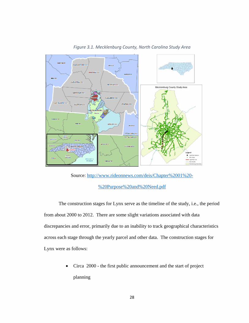
3.1 Study Area The study area of this thesis consists of the city of Charlotte, in Mecklenburg

County, North Carolina (Figure 3.1), with a focus on the Lynx light rail transit (LRT)

system and bus services. As is reasonably apparent, the light rail system has a limited

reach by itself while the bus system covers nearly the entire county. There are over three

thousand bus stops throughout Mecklenburg County and 15 light rail stations so far. On

top of the bus routes within the county, there are regional routes that extend outside the

county, but these routes will not be considered in this analysis.

Plans for the transit system began in 1984, when the Charlotte-Mecklenburg

Planning Commission suggested a light rail system from Uptown Charlotte to the

University of North Carolina (UNC) Charlotte campus, with the reasoning being that

growth of the campus would occur under the leadership of the third chancellor, James

Woodward. Additionally, physical improvement has continued to increase across the

campus in recent years, with new dorms and academic buildings (UNCC, 2013).

However, plans for this specific corridor would not move forward until after the Southern

corridor was completed and a feasibility study was planned, but never completed due to a

lack of available funds. Three years later, the mayor established a task force for studying

the possibility of a light rail system, with the result being eight different transit corridors

 

27  

radiating from Uptown Charlotte, based upon the consideration of population and

employment growth in the area. Ultimately, in 1991, $14 million were allotted for

acquiring abandoned rail right-of-way as it became available.

In 1998, Mecklenburg County voters approved a half cent sales tax increase that

would go directly towards funding the proposed LRT system. The corridor where the

system would eventually be completed was approved in 2000, with construction

commencing after groundbreaking in 2005 (Figure 3.1). After two years, the system was

completed and running, with ridership values exceeding projections by more than double.

Ridership has remained fairly consistent since opening, which is a good sign for any

expansion to a transit system, and certainly is good news for the previously mentioned

corridor planned from Uptown Charlotte to UNC Charlotte which was first proposed in

1984.

 

28  

Figure 3.1. Mecklenburg County, North Carolina Study Area 

Source: http://www.rideonnews.com/deis/Chapter%2001%20-

%20Purpose%20and%20Need.pdf

The construction stages for Lynx serve as the timeline of the study, i.e., the period

from about 2000 to 2012. There are some slight variations associated with data

discrepancies and error, primarily due to an inability to track geographical characteristics

across each stage through the yearly parcel and other data. The construction stages for

Lynx were as follows:

Circa 2000 - the first public announcement and the start of project

planning

 

29  

Circa 2005 - initial construction of the line began

Circa 2007 - the line first opened

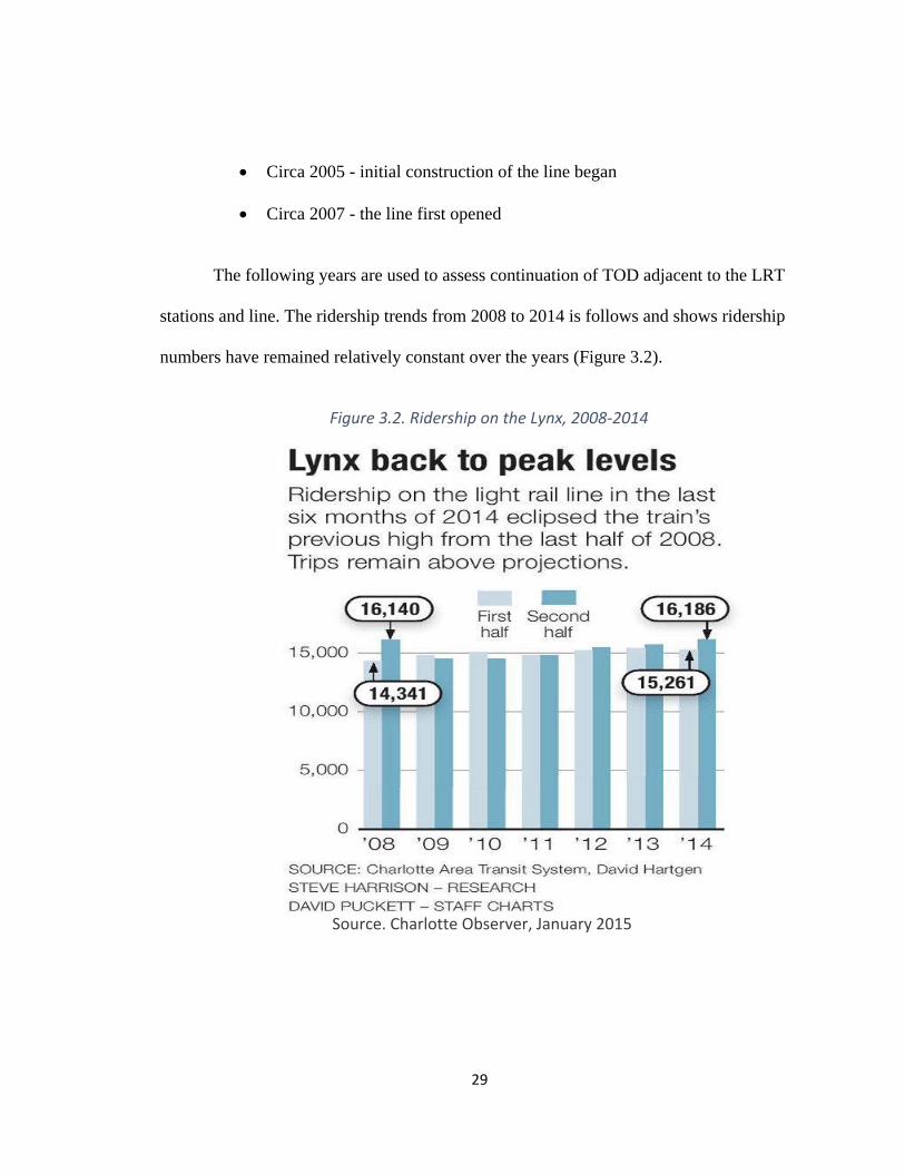
The following years are used to assess continuation of TOD adjacent to the LRT

stations and line. The ridership trends from 2008 to 2014 is follows and shows ridership

numbers have remained relatively constant over the years (Figure 3.2).

 

Figure 3.2. Ridership on the Lynx, 2008‐2014 

Source. Charlotte Observer, January 2015

 

30  

It is important to note that the first year ridership numbers (2007-2008) were

predicted to be around 8,000 but peaked rapidly after the LRT line began running at a

level of about 16,000. Although the numbers have not changed significantly since

opening, they began at twice the predicted rate and have far exceeded predictions

(Charlotte Area Transit System, CATS). These trends can be modeled to determine the

locations best served by improvements to the existing system and infrastructure, with the

capability of being scaled, adjusted and reused for other systems as both post-assessment

and as a predictive measure for communities to determine whether they would benefit

from future improvements.

 

3.2 Time Frame, Data Sources and Methodology

As mentioned above, the time frame of the study is between 2001 and 2012 for all

of the tax parcel data, 2000 and 2010 for the Census information and current bus and

LRT stop and route information. These are the time frames for which each of the

datasets was recorded and assessed. In other counties, tax parcel data are not recorded

every year, but at some regularly defined intervals. For example, Guilford County

updates their tax parcel data every eight years, which does not provide the level of detail

available for Mecklenburg or Wake County, two counties that will be included as control

groups in future expansions of this model.

Data for this research primarily comes directly from the GIS department of

Mecklenburg, NC

(http://charmeck.org/mecklenburg/county/LUESA/GIS/Pages/Default.aspx), a site

dedicated to providing a variety of free and unobstructed data. The data types involved in

 

31  

this research project include tax parcel and other property data before, during and after

the time period, boundary data files, railroad data, Census data for 2000 and 2010, aerial

and ortho-imagery, highway, major road and basic street data, along with many other

relevant data types and files.

In addition to the main county web portals, data were also received directly from

Mecklenburg’s GIS office, NCDOT, NC Rail and many other sources throughout the

state. Many of these data are not used directly in the modeling process, but are instead

used for the purposes of assessing existing infrastructure, e.g., abandoned or disused

railroad corridors that could be upgraded or transformed for the purposes of new or

improved modes of public transportation. This type of assessment can be used to

positively influence legislators and public interest groups with respect to the benefits of

planning and development of existing locations. It is likely that there are cases for

improving upon what already exists, rather than opting for less well defined, loose

development patterns that would likely create additional costs through a need for

expanding water and sewer lines and creating additional road and sidewalk extensions.

The six primary variables that have been identified by past empirical research to

be those of highest importance for TOD to occur are used for this thesis:

1) Land Value Change

2) Housing Unit Density Change

3) Bus Station Density

4) Accessibility

5) Population Change

 

32  

Each variable was converted to a raster, i.e., a pattern of scanning lines covering a

particular image area, by way of two processes, inverse distance weighted interpolation

(IDW) or direct raster to polygon function, available within ArcGIS®, a well-known GIS

software application developed by ESRI. The IDW tool can only be used with point

files, so all of the relevant tax parcel level variables (land value, housing units, vacant

property, population change) needed to be converted into points based on the geometric

center of each record (centroid) and then have the IDW analysis performed. This process

created a smooth raster image that displayed spatial relationships between each point, i.e.,

tax parcel, and the variable as a pixel value with each pixel defined to be 30 x 30 ft

(~9.1x 9.1m).

For the second method, the polygon shapefile was directly converted to a raster

image using the raster to polygon tool, again with a 30 x30 ft (~9.1 x 9.1m) pixel size and

the pixel value being defined as the variable value. This method was used for the

accessibility and bus station density variables. It did not create a raster image that

displayed the spatial relationships, but rather an exact duplicate of the related vector file.

For these variables, the values utilized were combinations of other values, providing a

form of analysis prior to becoming rasterized.

The model utilized in this research was developed from the ground up, and

verified from similar studies analyzing and predicting bike share ridership. The model

consisted of three stages:

a) Convert a polygon file into a point file

 

33  

b) Convert a vector point file into a raster image based on a specific variable value

using a spatial interpolation function if possible

c) Reclassify the raster image into a point system.

Note: For all aspects of the analysis, ArcGIS® was utilized for its spatial analytical

toolsets.

After all six variables were converted into raster images and reclassified to be part

of a point system analysis, where low values represent TOD and high values do not, all of

the layers were overlaid on one another and combined. The outcome was a raster image

that provided a clear depiction of locations where TOD was most likely to be located.

Using this entire process provided the key for determining the effectiveness of each

individual variable, as well as the collective in performing the evaluation portion of the

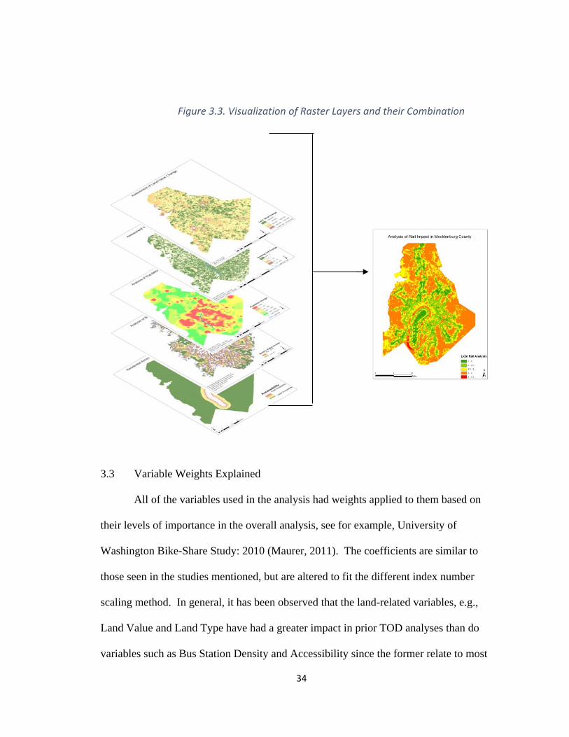
analysis on the urban landscape. Figure 3.3 visualizes the process by which rasterized

vector data can be added together. This method includes tax parcel level data, created

vector data and Census Block Group level data. Different datasets with overlapping

geographic extents can be combined using a raster calculator function to develop one

comprehensive raster image.

 

34  

3.3 Variable Weights Explained

All of the variables used in the analysis had weights applied to them based on

their levels of importance in the overall analysis, see for example, University of

Washington Bike-Share Study: 2010 (Maurer, 2011). The coefficients are similar to

those seen in the studies mentioned, but are altered to fit the different index number

scaling method. In general, it has been observed that the land-related variables, e.g.,

Land Value and Land Type have had a greater impact in prior TOD analyses than do

variables such as Bus Station Density and Accessibility since the former relate to most

Figure 3.3. Visualization of Raster Layers and their Combination

 

35  

forms of transit while the latter two relate only to the bus system. In order to obtain a

more normalized output that is more amenable to evaluation of resulting index values,

Accessibility and Bus Stop Density were given a higher weight with a coefficient of 0.3

and Land Value and Land Type were given lower weights, i.e., coefficients of 0.1. . This

yielded a magnified impact of the key variables understood to be related to public transit

and it was clearly evident that these variables had the greatest impact in and around

Uptown Charlotte.

3.4 Methodology

The overall methodology for this research is to develop a model that is derived

from empirically assessed, observed and implemented calculations and variables for the

purposes of analyzing public transit infrastructure with respect to all of the benefits and

costs new and improved systems have and will incur over their lifespan. As noted in the

introduction and literature review sections, much of the research and analyses over the

past eighty years have neglected to tie together all of the previously assessed factors

believed and shown to influence or be influenced by public transit infrastructure

investments. The model discussed and developed in this research is believed to be

capable of bridging the gap and providing a means to assess systems at many scales for

these purposes, as similar models for studies with similar structures have been shown to

work successfully (Maurer 2011; Seattle 2010).

Using raster images rather than vector data for the evaluation, with the inclusion

of spatial analysis techniques such as inverse distance weighted (IDW) interpolation,

provides an opportunity to conduct analysis at micro-scale, with a higher resolution of 30

 

36  

x 30 ft (~9.1 x 9.1m), that Block Group level analysis cannot offer. Additionally, many

of the variables were obtained from tax parcel data, which provides much higher

resolution than that provided by the use of Census data. Only one of the variables is at

the Census Block Group (BG) level. All of the temporal data were assessed using IDW,

which took into account the spatial relationships between each and every point, creating a

smooth, continuous raster surface, using a resolution of 30 x 30 ft (~9.1 x 9.1m). Static

data, e.g., accessibility, were converted directly into raster images, with the same

resolution, with the impact of the static data remaining in a linear pattern.

A gap exists because researchers have failed to develop models and studies that

assess all of the empirically studied factors together, thereby only looking at a part of the

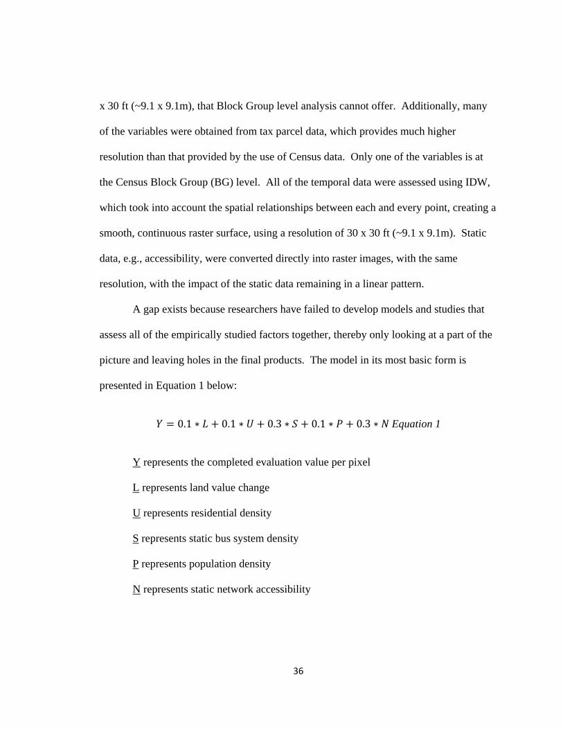
picture and leaving holes in the final products. The model in its most basic form is

presented in Equation 1 below:

0.1 ∗ 0.1 ∗ 0.3 ∗ 0.1 ∗ 0.3 ∗ Equation 1

Y represents the completed evaluation value per pixel

L represents land value change

U represents residential density

S represents static bus system density

P represents population density

N represents static network accessibility

 

37  

Each variable was rasterized, either by direct conversion or through formulas that

yield raster images, and reclassified and combined through the use of Raster Calculator

function, a method that has been utilized for several similar projects, such as a bike share

feasibility study (University of Washington, March 2010), where several variables were

assessed together for the purposes of utility and infrastructure improvements on a large

scale. In the case of U of Washington’s feasibility study, it was for much of the greater

Seattle region, with determinations of several different phases of the installation,

beginning with localities that were most in line with characteristic requirements, e.g.,

high population density and work and entertainment trip output, plus ready access to

universities and student populations, although this was given a lower weight against

overall population density to reduce double counting errors.

This type of approach has been utilized in previous thesis research including the

recent work by Maurer (2011) in her suitability assessment of Sacramento and

Minneapolis for the purposes of installing bike-share sites. Maurer’s approach was

multi-staged and used outputs from Minneapolis to help in the Sacramento assessment,

but it included similar data types, as well as factors and methodology akin to those seen

in this research. With validation of this approach established, the research methods

utilized to measure land value change in this thesis will be discussed in a step-by-step

manner in the Results section (CHAPTER IV).

3.4.1 Change in Land Value

The methodology for assessing how land value changes over a given time period

is still somewhat in question in terms of an ideal way that eliminates the most amount of

 

38  

error. For the purpose of this work, the original method, prior to any complex or

empirically verified calculation, was to aggregate the parcel data to a Census Block

Group scale in the interest of generating data more quickly, convert the tax parcel data to

a raster format based on the land value characteristic and divide the final year of the study

by the first year of the study, (2012 / 2001). This derivation resulted in a magnitude

value, where the value of each cell was X number of times different from the original

value of the cells, indicative of positive, negative or no change in value over the period.

The equation for assessing change in land value is described by displaying the

overall change for each parcel (Equation 2):

2012 2002 Equation 2

This is useful for identifying the changes in key location points, such as the urban core

and higher density suburban centers where public transit infrastructure is necessary for

many residents to connect home to work trips without the use of a personal vehicle. This

format is also supported by the work of Batt (2001) in his post-assessment of value

capture as a policy tool. Whereas Batt’s study was for a section of highway, the

assessment detailed land value adjacent to the Northway (New York City), comprising a

similar situation with which to base usage of the above equation.

The improved method for determining land value change is to utilize the process

of Inverse Distance Weighting (IDW). The tool in ArcGIS® requires input of a point file

and specific column from within that file in order to perform the analysis. Additionally, a

 

39  

cell size can be input, either from a file or manually. In this case, a cell size of 30 x 30

feet (9.1 x 9.1 m) was used.

3.4.2 Change in Housing Style and Land Uses

The use of housing units, over specific land use types, e.g., single family

residential or rental, was chosen for this model to represent the changes in housing types

and land uses because it provides a clear representation of housing type. If there are

many housing units per parcel in a given area then it can be accurately deduced that there

are large apartment and multi-family complexes present, since the data are related to

individuals. If there are no housing units on a given parcel, then the property is used for

purposes other than residential. These aspects, coupled with land valuation, can indicate

the presence of corporate parks, business centers and large scale retail developments. As

this model is primarily being used to identify the coordination of TOD with any public

transit improvement, the apparent segregation of these types, or presence of mixed uses,

i.e., if high land values are coupled with high numbers of housing units, can be used to

determine how successful efforts have been or could be to create the necessary

partnerships between government, public organizations and private interests for long term

success of systems.

Assessing the changes in housing units over the time period will function much

the same way as the previous variable, by utilizing the housing units column found in the

parcel level data and subtracting the housing units for the starting year from the most

recent year (2012), thereby getting a negative, positive or zero number for the exact

 

40  

change over the entire time period. To assess residential density, Equation 3 was used to

provide a good assessment of change in residential density across the entire county.

2012 2001 Equation 3

Again, IDW was used to interpret how housing units across the entire county

changed over the duration of completion of the Lynx LRT, with the inclusion of the LRT

rail line as a barrier to provide support of the relationships between proximity to LRT and

changes in housing unit density.

The means by which this characteristic was verified was to perform the operation

for the entire county for all properties, followed by an analysis of the county for the

presence of the vacant properties. All of the properties were first converted to points

based on the centroid of the polygons. Next, the point file would have an IDW

interpolation performed to create a continuous surface representation of all housing units.

The variables for the IDW procedure that were changed from the default were the

resolution, which was set for 300 feet (91.4 m), and the polyline barrier, where the LRT

rail line was input. Using the rail line as a barrier served to represent the fact that

properties exist surrounding the line, not crossing it.

3.4.3 Bus Transit Station Density

This factor relates to the fact that the establishment of an LRT line in the higher

density areas of a city will only be walkable by a small percentage of the total population.

Within a radius of the line of up to one and a half miles (two and a half kilometers) the

improvement will provide great accessibility and mobility. However, it is expected that

 

41  

much of the city or county will not have any direct connection to the improvement

without a personal vehicle or additional mode of transportation. To account for this

deficiency, having significant bus or bicycle facility density throughout the entire study

area would provide the necessary linking factor between distant residents and the new

improvement. Providing bus stop locations at key population centers would serve to

provide both accessibility and mobility to the entire study area, instead of just within the

walking adjacency buffer, on top of bridging the gap between the “last mile,” i.e., the

length between where commuters typically get off one form of transport to get on another

in order to reach employment.

For accomplishing this level of analysis, Network Analyst in ArcGIS® was used to

develop a network-accurate value field using the tool Service Area. By using Service

Area, coupled with the number of bus stops located within each buffer zone, it is possible

to assess density, since it provides a real world assessment of the service area for the bus

system by utilizing the road network, instead of a straight-line Euclidean distance

analysis.

The total range of the network analysis was 3 miles (5 kilometers) from the

nearest bus stop. This was included because it extends the reach of the system enough to

ensure the most coverage for the final analysis of the system. In reality, anything beyond

1.5 mile (2.5 kilometers) would be unlikely for residents to walk on a daily basis for

either work or personal activities. The most relevant parts of the service area analysis

are those of:

1) 0.25 miles (0.4 kilometers)

 

42  

2) 0.5 miles (0.8 kilometers)

3) 0.75 miles (1.25 kilometers)

4) 1.0 miles(1.6 kilometers)

5) 1.5 miles (2.5 kilometers)

Note: 2 miles and 3 miles (3.25 and 5 kilometers) were also included, again to extend

the reach of the model for the final overlay.

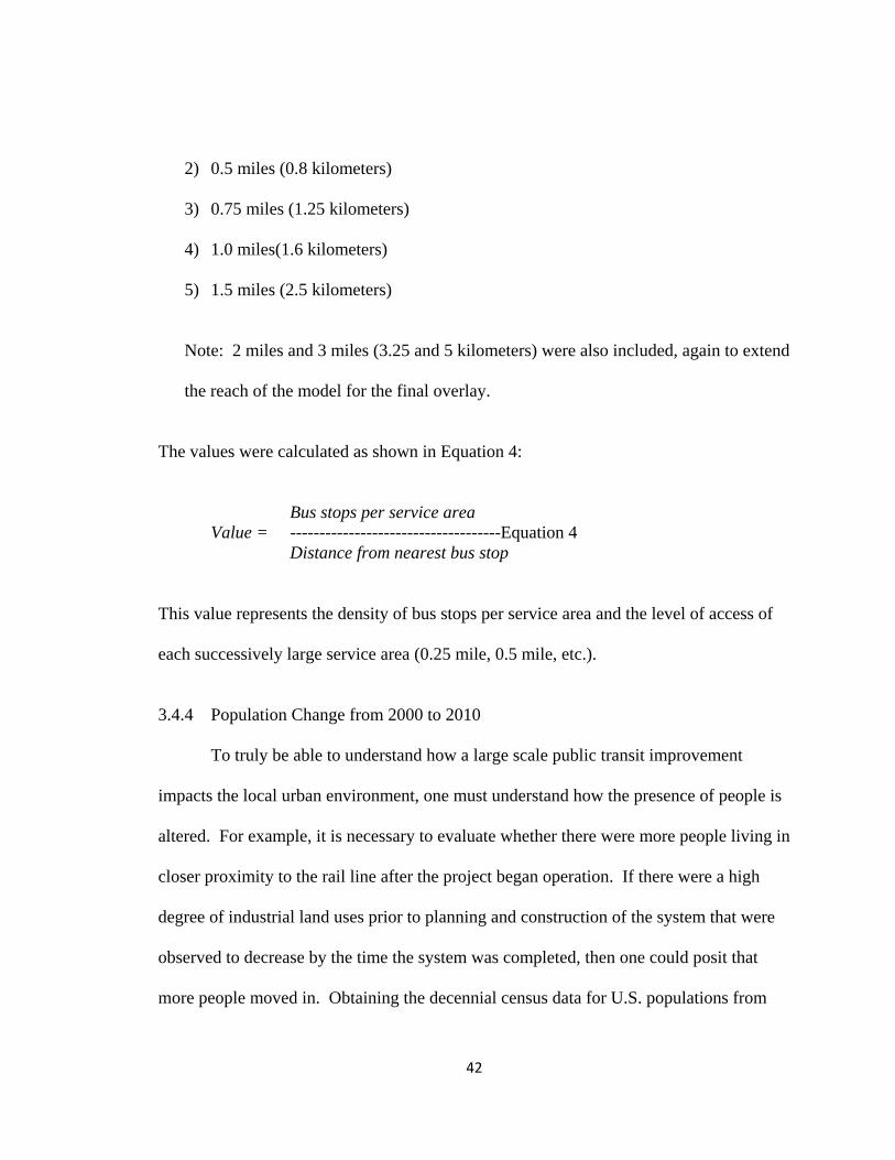
The values were calculated as shown in Equation 4:

Bus stops per service area

Value = ------------------------------------Equation 4 Distance from nearest bus stop

This value represents the density of bus stops per service area and the level of access of

each successively large service area (0.25 mile, 0.5 mile, etc.).

3.4.4 Population Change from 2000 to 2010

To truly be able to understand how a large scale public transit improvement

impacts the local urban environment, one must understand how the presence of people is

altered. For example, it is necessary to evaluate whether there were more people living in

closer proximity to the rail line after the project began operation. If there were a high

degree of industrial land uses prior to planning and construction of the system that were

observed to decrease by the time the system was completed, then one could posit that

more people moved in. Obtaining the decennial census data for U.S. populations from

 

43  

the Census Bureau was paramount for determining whether these assumptions were

correct.

Ordinarily, when one obtains data for comparison from two different Census

years, e. g., Census 2000 and Census 2010, there would be errors with comparing the two

spatial datasets. This is primarily because the numbers, sizes and shapes of Census

geographies change each time. Where this would normally be an issue, UNC Greensboro

purchased data products from Geolytics, a company that takes Census data and edits

previous years’ data so that they match up with the current (Census 2010) decennial

Census geography. For the purposes of this research, where mismatched data sets would

have created holes in the final product, the Geolytics products were invaluable for this

stage in the analysis process.

While using Block Groups (BG) may often times provide less accurate data than

using Tax Parcel level information, Mecklenburg County has the benefit of having

smaller Block Groups in and around the majority of the existing Lynx LRT line. This

means that although the geographies between Tax Parcels and Block Groups will not

match up, when using the IDW analysis function, the spatial relationships between BGs

closer to the central area of Mecklenburg County will be in greater agreement. BGs

farther from the center are generally larger, and will be more loosely related, with less

overall influence on the complete analysis.

For the purposes of this analysis, it was composed of three stages:

 

44  

1) Obtaining Census 2010 data from the U.S. Census Bureau and joining it with

population data from the American FactFinder website

2) Downloading the Census 2000 data in 2010 boundaries through the Geolytics

databases on the UNC Greensboro library website and joining it into the Census

2010 shapefile

3) Converting the shapefile to points, followed by performing an IDW analysis on

the points.

For the first step, it was straightforward to get the Census 2010 Block Groups file

from the Census Bureau, and download the population dataset for 2010 in Mecklenburg

County from the American FactFinder website. Joining the datasets together presented

no difficulties since they both had the required database field for the BGs.

The Geolytics database has a simple web format that allows one to select the

geography, location and requisite data, and then download it in the appropriate cell

format within Excel®, i.e., a comma separated variable, however, the key variable for the

joining process needed to be converted to a text format using the TEXT function. This

added an extra step before it could be joined to the existing BG 2010 shapefile in

ArcMap®. Once this step was finished, it was successfully joined and fields were added

to the attribute table for calculating the change per BG from 2000 to 2010. The third step

was to convert the BG shapes into points, using the feature to points function in

ArcMap® and to perform an IDW.

 

45  

3.4.5 Transit Station Accessibility in Mecklenburg County

Transit accessibility is the measure of one’s ability to get from point A to point B

utilizing available modes of transportation. For almost all cities in the United States, this

primarily revolves around residents’ access to the road network using personal vehicles

or riding a bus, but it can also include a sidewalk/greenway network for walking and

bicycling. Very little has been done to develop methods for assessing light rail transit

accessibility, as LRT systems are not widespread in the US. Additionally, roadway

networks are often developed in a fashion that does not typically include any temporal

aspect of a transit plan, making it almost impossible to determine how the network

changed during the lifetime of any transit improvements.

For the purposes of this research, accessibility is the measure of road network

density around each light rail station for the entire county. The density measure is

developed through the TIGER/Line roads file from the Census Bureau, clipped to the

shape of the county and a length field is calculated for each individual road record. A

multi-ring buffer was created around the individual light rail stations for the following

distances from a Station (in miles):

0.25, 0.5, 0.75, 1.0, 1.5, 2.0, 3.0 and 25.0 mi

(0.40, 0.80, 1.25, 1.60, 2.50, 3.25, 5.00 and 41.0 in km)

The final distance (25 miles/41 km) was used to ensure that the buffer covered the

entirety of the county for the final calculation. The most relevant distance values for this

buffer were the values from 0.25 miles (0.40 km) up to 1.0 miles (1.6 km), which are

 

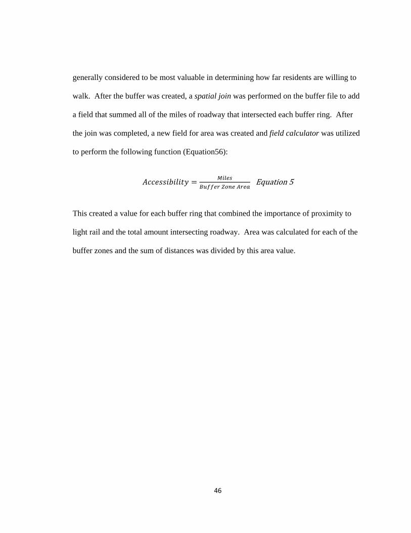
46  

generally considered to be most valuable in determining how far residents are willing to

walk. After the buffer was created, a spatial join was performed on the buffer file to add

a field that summed all of the miles of roadway that intersected each buffer ring. After

the join was completed, a new field for area was created and field calculator was utilized

to perform the following function (Equation56):

Equation5

This created a value for each buffer ring that combined the importance of proximity to

light rail and the total amount intersecting roadway. Area was calculated for each of the

buffer zones and the sum of distances was divided by this area value.

 

47  

CHAPTER IV

RESULTS AND ANALYSIS

4.1 Evaluation of Benefits from Transit Development in Mecklenburg County

4.1.1. Change in Land Value

The result of this analysis was a raster image that displayed hotspots of land value

increase and decrease over the ten year time period being studied (2000-2010). These

results were compared with those obtained by converting the parcels directly into a raster

image with the function, polygon to raster, followed subsequently with a raster

reclassification of land values into five categories. Although the latter method took less

time, there was little analysis of relationships between value and space, making the result

little more than a visualization of raw data. By using the IDW function, an interpolated

surface was created that links the basic principles of space and value, providing an

interpretation of how proximity to light rail could have impacted the property values of

adjacent land. The nature of proximity to light rail was denoted by the inclusion of the

rail line as a barrier for the process.

Using the IDW method of analysis resulted in fewer human input errors from

unnecessary conversions and aggregations. Additionally, the result of the process was a

surface without holes, as IDW determines relationships over areas where no data were

present, making statistical assumptions for what would likely exist in the gaps. With

 

48  

regard to the final calculation of all variable raster images, this yields a composite image

with a larger coverage area and fewer incomplete areas.

Values that were less than 1 indicated a decrease over time, a value of 1 meant no

change and any higher value indicated an increase. Some areas showed changes of over a

hundred times in land value, especially along the Lynx transit corridor in Mecklenburg.

Unfortunately, due to the aggregation, the changes appeared consistent along much of the

corridor, making it difficult to determine the smaller scale changes occurring in specific

locations such as Uptown Charlotte and the housing sector along the South end of the

line. As a result, it was determined that the method of using the higher resolution tax

parcel data is more suitable. Additionally, the errors caused be aggregating the data were

too large to accept as accurate.

Hot spots of extreme land value increases throughout Mecklenburg County were

found to be where they were expected, i.e., Uptown Charlotte, as well as in the shopping

center located approximately 8 miles (13 kilometers) north of Uptown. There were a few

other sections with considerable land value increases, one of which was located 4 miles

(6.5 kilometers) northwest of the central segment of the Lynx line. The overall evaluation

provided by this method is that almost the entire 2 mile (3 kilometer) buffer saw either

positive or neutral change over the time period.

For the reclassification of the raster image, the values were classified into the

same dollar value categories as in Figure 4.1 below:

1) $5,000,000 – $58,000,000

2) $1,000,000 – $5,000,000

 

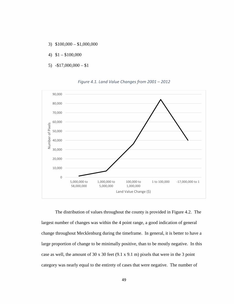
49  

3) $100,000 – $1,000,000

4) $1 – $100,000

5) -$17,000,000 – $1

 Figure 4.1. Land Value Changes from 2001 – 2012 

 

   

The distribution of values throughout the county is provided in Figure 4.2. The

largest number of changes was within the 4 point range, a good indication of general

change throughout Mecklenburg during the timeframe. In general, it is better to have a

large proportion of change to be minimally positive, than to be mostly negative. In this

case as well, the amount of 30 x 30 feet (9.1 x 9.1 m) pixels that were in the 3 point

category was nearly equal to the entirety of cases that were negative. The number of

0

10,000

20,000

30,000

40,000

50,000

60,000

70,000

80,000

90,000

5,000,000 to58,000,000

1,000,000 to5,000,000

100,000 to1,000,000

1 to 100,000 ‐17,000,000 to 1

Number of Pixels

Land Value Change ($)

 

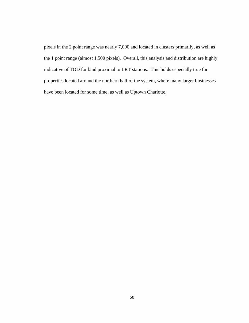
50  

pixels in the 2 point range was nearly 7,000 and located in clusters primarily, as well as

the 1 point range (almost 1,500 pixels). Overall, this analysis and distribution are highly

indicative of TOD for land proximal to LRT stations. This holds especially true for

properties located around the northern half of the system, where many larger businesses

have been located for some time, as well as Uptown Charlotte.

 

51  

Figure 4.2. Analysis of Total Land Value Change, 2002 ‐ 2012 

 

52  

4.1.2 Changes in Housing Unit Density

At the northern most segment of the Lynx line, surrounding a cluster of the last

five stations, there were significant increases in housing units. This coincides with the

area where land value changes were highest along the corridor, albeit in select areas

within that region. In one area, the pixel values range from 50 to 230 new housing units

and in other clusters the values range between 25 and 50 per pixel. All of these

significant changes occur within 0.5 miles (0.8 km) of any one station in this region.

For the reclassification of the housing unit density raster, the classifications

remained the same from the map of housing unit change, Figure 4.3:

1) 50 - 230

2) 25 - 50

3) 1 - 25

4) 0 – 1

5) -220-0

 

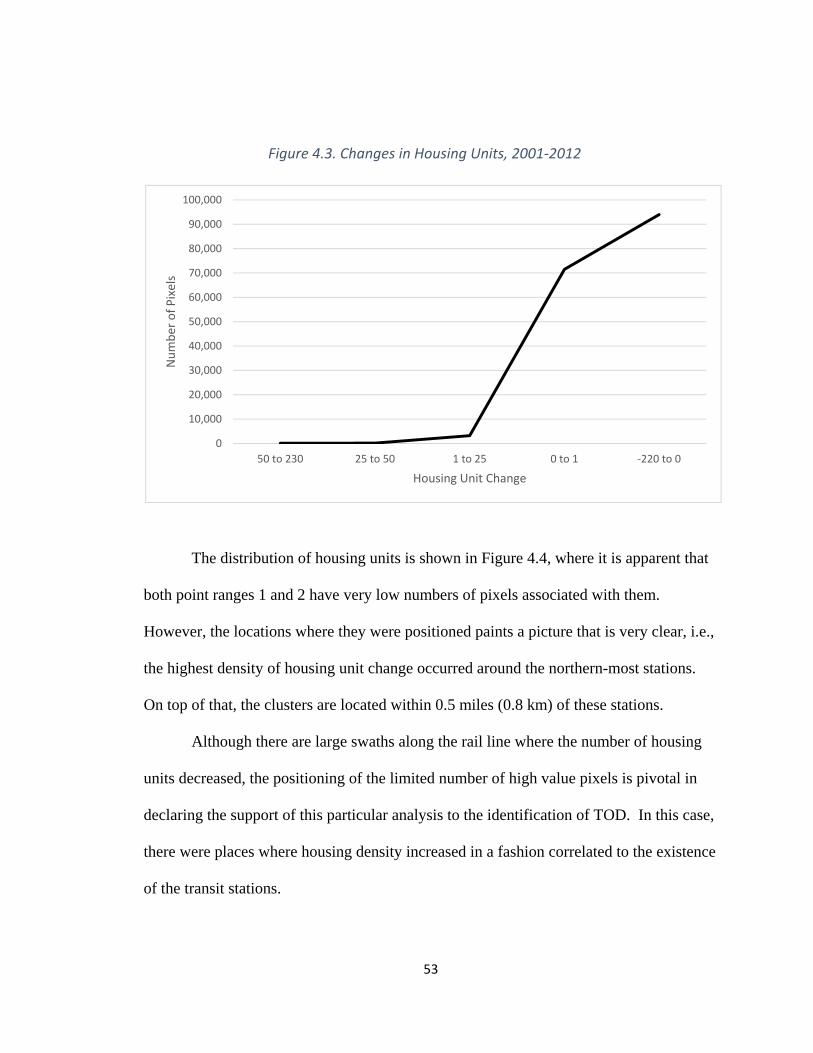
53  

The distribution of housing units is shown in Figure 4.4, where it is apparent that

both point ranges 1 and 2 have very low numbers of pixels associated with them.

However, the locations where they were positioned paints a picture that is very clear, i.e.,

the highest density of housing unit change occurred around the northern-most stations.

On top of that, the clusters are located within 0.5 miles (0.8 km) of these stations.

Although there are large swaths along the rail line where the number of housing

units decreased, the positioning of the limited number of high value pixels is pivotal in

declaring the support of this particular analysis to the identification of TOD. In this case,

there were places where housing density increased in a fashion correlated to the existence

of the transit stations.

0

10,000

20,000

30,000

40,000

50,000

60,000

70,000

80,000

90,000

100,000

50 to 230 25 to 50 1 to 25 0 to 1 ‐220 to 0

Number of Pixels

Housing Unit Change

Figure 4.3. Changes in Housing Units, 2001‐2012 

 

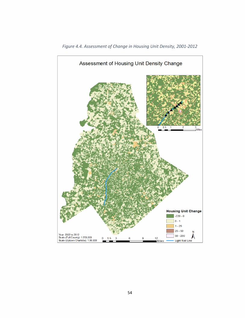
54  

Figure 4.4. Assessment of Change in Housing Unit Density, 2001‐2012 

 

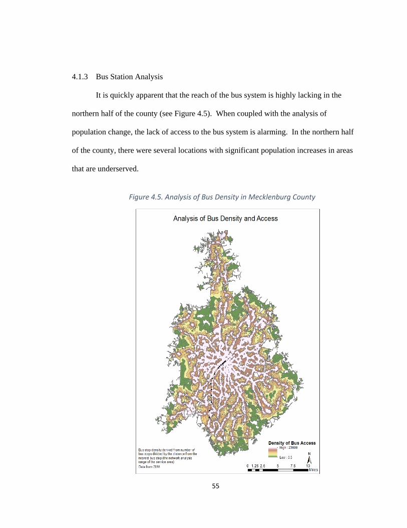
55  

4.1.3 Bus Station Analysis

It is quickly apparent that the reach of the bus system is highly lacking in the

northern half of the county (see Figure 4.5). When coupled with the analysis of

population change, the lack of access to the bus system is alarming. In the northern half

of the county, there were several locations with significant population increases in areas

that are underserved.

Figure 4.5. Analysis of Bus Density in Mecklenburg County 

 

56  

The complete lack of bus stops outside of the 0.25 miles (0.4 km) service area is

apparent. Over 3,500 of the 3,589 total bus stops in the county lie within 0.25 miles (0.4

km) service area. Outside of the service area, the density of stops decreases to less than

1% of the total, and continues to decrease. For more of the county to be considered

transit-oriented, the reach of the bus system needs to be increased to reach areas where

buses do not currently go, and the density of bus stops within each service area should be

enhanced.

4.1.4 Population Change

What results from the above analysis is a clear indication of positive change along

the corridor, with the Uptown Charlotte area showing significant change within about 1.0

mile (1.6 km) of the northern–most stations. Even along the southern tip there were

significant increases within a 1.0 mile (1.6 km) or more of the stations. This is highly

indicative of changes in land use from industrial to retail and residential uses. In the area

outside of 1.0 mile (1.6 km) of the northern most station, there were apparent decreases,

forming a ring around the station where large swaths of residents apparently moved out.

What can be taken away from this particular analysis is that the evidence shows

clear signs that proximity to rail stations, mostly in the northern and southern tips of the

system, served as a key draw for residents, i.e., a reliable means of public transportation

is desirable. Additionally, using the LRT line as a barrier since no resident could live on

the rail line, only near it, the analysis showed more positive relationships proximal to the

interior stations of the system.

 

57  

Analysis of population changes along large scale public transit improvement

projects has been shown to relate the human dimension of impacts that these projects may

have. Clearly, the presence of a new transit mode positively influenced residents’

decisions to move closer to rail stations, at least for the majority of the stations. The

southern tip of the system displayed overall higher changes in population, yet, the

northern stations had dense, localized increases within 2.0 miles (3.25 km) of the

stations, indicative of high residential increases.

As with the other assessments above, the population change raster was

reclassified into the same point system, with the value ranges as given below:

1) 1,000 to 3,600

2) 500 to 1,000

3) 150 to 500

4) 1 to 150

5) -2,200 to 1

The distribution of the value ranges is provided in Figure 4.6. Most of the pixel values

found in the county were positive, with the most important finding being the close

relationship of high population increases within 1 mile (1.6 km) of a transit station. Even

stations along the central part of the rail line showed pockets of population increases. On

the East side of the rail line, more than 1.0 mile (1.6 km) beyond stations, there were

considerable increases in population that would be somewhat counter to what some

 

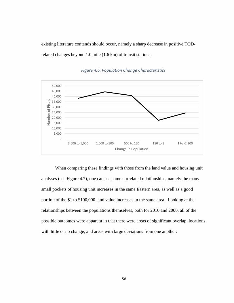
58  

existing literature contends should occur, namely a sharp decrease in positive TOD-

related changes beyond 1.0 mile (1.6 km) of transit stations.

When comparing these findings with those from the land value and housing unit

analyses (see Figure 4.7), one can see some correlated relationships, namely the many

small pockets of housing unit increases in the same Eastern area, as well as a good

portion of the $1 to $100,000 land value increases in the same area. Looking at the

relationships between the populations themselves, both for 2010 and 2000, all of the

possible outcomes were apparent in that there were areas of significant overlap, locations

with little or no change, and areas with large deviations from one another.

0

5,000

10,000

15,000

20,000

25,000

30,000

35,000

40,000

45,000

50,000

3,600 to 1,000 1,000 to 500 500 to 150 150 to 1 1 to ‐2,200

Number of Pixels

Change in Population

Figure 4.6. Population Change Characteristics 

 

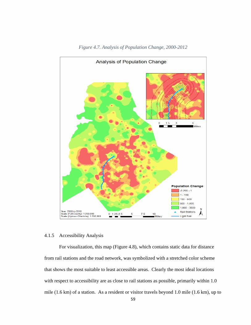
59  

Figure 4.7. Analysis of Population Change, 2000-2012  

  

 

4.1.5 Accessibility Analysis

For visualization, this map (Figure 4.8), which contains static data for distance

from rail stations and the road network, was symbolized with a stretched color scheme

that shows the most suitable to least accessible areas. Clearly the most ideal locations

with respect to accessibility are as close to rail stations as possible, primarily within 1.0

mile (1.6 km) of a station. As a resident or visitor travels beyond 1.0 mile (1.6 km), up to

 

60  

3.0 mile (5 km), accessibility drops substantially, with network access beyond that being

minimal.

It can be assumed that road network density remains relatively constant

throughout the county. With this assumption in mind, the fact that residential

accessibility decreases so much for the county not within close proximity to rail stations

is not clear. Utilizing the area of each zone as the normalizing factor means that the

magnitude of the differences in size should be minimized when comparing the density of

road mileage within each zone. This method yielded results that clearly indicate that the

density of road mileage, not unlike the analysis of the bus system, is centered on Uptown

Charlotte, with a steep drop-off in general accessibility for much of the county.

 

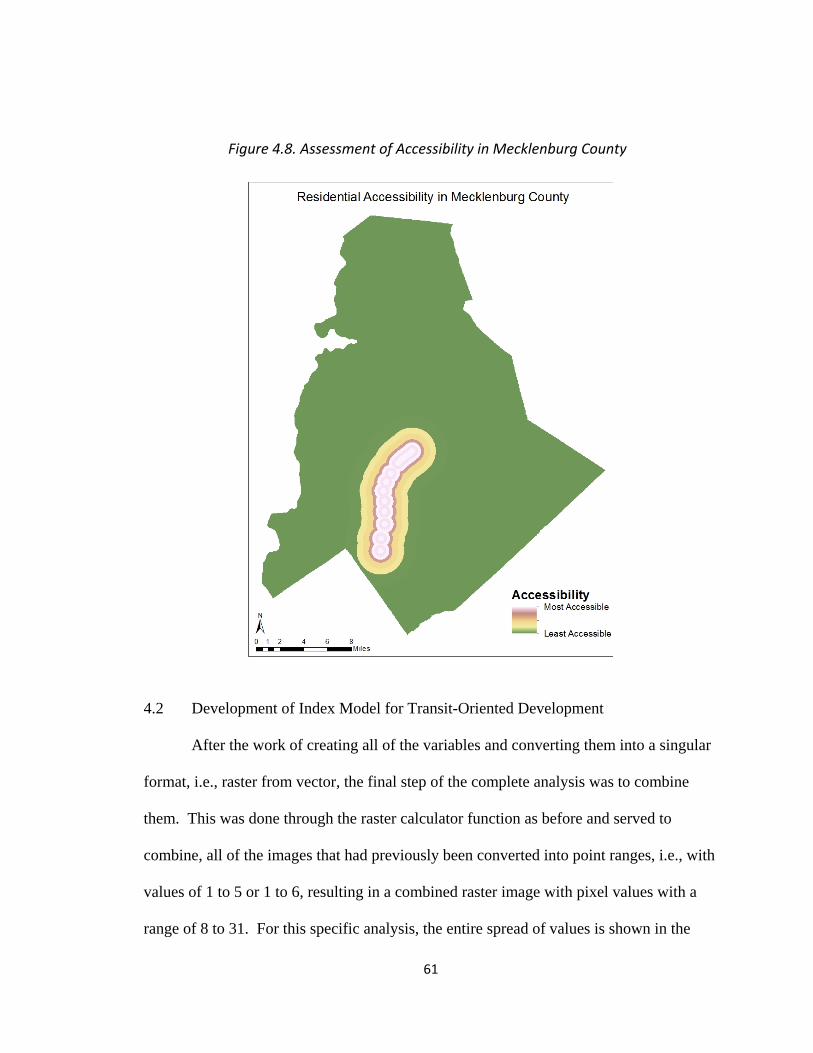
61  

4.2 Development of Index Model for Transit-Oriented Development

After the work of creating all of the variables and converting them into a singular

format, i.e., raster from vector, the final step of the complete analysis was to combine

them. This was done through the raster calculator function as before and served to

combine, all of the images that had previously been converted into point ranges, i.e., with

values of 1 to 5 or 1 to 6, resulting in a combined raster image with pixel values with a

range of 8 to 31. For this specific analysis, the entire spread of values is shown in the

Figure 4.8. Assessment of Accessibility in Mecklenburg County 

 

62  

legend since an accurate and complete visualization of TOD in Mecklenburg County was

the goal of this work.

Based on the prior discussion and calculation of TOD, the number value ranges

can be assessed in the following TOD groups:

1) TOD Present – 8 to 15

2) TOD Emergent – 16 to 23

3) TOD Not Present – 24 to 31

Reasoning for deciding to have the index go from lower to higher, with the lower

values representing TOD was based on other similar studies where indices were utilized,

with a similar numbering scheme (Maurer 2011, Seattle 2010). The values were

displayed in these three categories for the purpose of distinguishing distinct areas within

the county. The areas were not intended to overlap with specific cities or interest areas,

however, the results were positively in line with hypothetical expectations. TOD was

present around the northern stations, around some of the southern stations, with mixed

results in between. Additionally, there were some potential TOD developments apparent

in the region north of the Lynx, where a large shopping center was constructed near the

bus line and less than 10 miles (16 km) from Uptown Charlotte. Areas near UNC

Charlotte showed very strong signs of TOD, as well as large swaths of emerging TOD

along the majority of the planned NE extension line.

 

63  

4.2.1 The Value of Raster Conversion

The question remains of why raster conversion was chosen over leaving the data

in a vector format, i.e. leaving the data scale as Block Groups or tax parcels. Vector data

has uses primarily when a researcher needs to be able to join data for one dataset from

multiple years, as in comparing Census Block Group vector data for the 2000 and 2010

decennial Census. The population demographic data needs to be joined to the Census

Block Group vector data, after which, the changes in demographics can be assessed

between the two Censuses. The results show discrete relationships at a macro-scale

within regions and groups. Being able to convert the data from vector to raster format

through the use of an analysis tool, like Inverse Distance Weighted (IDW) analysis,

provides a means to perform a micro-scale assessment of each variable at a user set

resolution. However, a more complex analysis of multiple variables can be performed

using the Raster Calculator tool within ArcGIS®, providing visible results that cannot be

reached through regular vector data analysis. This is the general format for the index

model explored in this research.

A key aspect of this method is the wide range of scales possible, as well as the

continuous surface. The IDW tool provides the user with the ability to set their own

resolution and this should be determined based on the data provided. For the purposes of

this research and as a result of the majority of variables coming from the tax parcel

datasets, the IDW resolution is 30 feet by 30 feet (~9.1m by 9.1m). The tax parcel data is

reasonably accurate at that level and is able to provide a micro-scale analysis across the

entire county.

 

64  

Following the research format of Maurer (2011) and Washington (2010) which

detailed similar index studies for bike share systems in Minneapolis/St. Paul and Seattle,

respectively, the index model described in this research required raster format variables

to develop a continuous surface analysis. This method, which assesses the spatial

relationships between points as well as the variables themselves, has been shown to

provide a clear depiction of how the variable relates to the area in question. In this case,

the raster analysis, developed through the use of Inverse Distance Weighted (IDW)

analysis, showed relationships between each variable and the Lynx light rail system.

4.3 Existing TOD in Charlotte

Figure 4.9 shows the results, in which it is apparent that there is a dense collection

of points in the northern area of the Lynx and many smaller groupings of TOD along the

West side of the line, further south. The inset map shows the North section of the rail

system, with rail line and stations, as well as a multi-ring buffer. The buffer shows the

scale of TOD within certain proximities of stations, with density of TOD decreasing

dramatically the further away one gets from a station. As shown in the map, places of

TOD determined by the index equation are circled, with eight locations showing up in the

evaluation. Two of the areas were directly proximal to the Lynx LRT system, with the

highest density area of TOD being in the Uptown Charlotte area.

In the inset map of the northern half of the LRT, which was included to display

the properties evaluated in the analysis within 1.0 mile (1.6 km) of the transit stations,

there is a high density area of TOD within a 0.25 mile (0.4 km) of the northernmost

station, with decreasing importance out to 1.6 km and no importance beyond that. The

 

65  

numbers range from 8 to 15 within a 0.4 km, mostly 16 to 23 out to 1.0 mile (1.6 km) and

24 to 31 beyond the rest of the boundary. This supports the idea of the benefits of

proximity to transit stations decreasing nearly exponentially with distance from the

station, with the greatest benefits being observed extremely closely to the stations. There

appear to be no benefits outside of a distance of 1.0 mile (1.6 km) from stations.

 

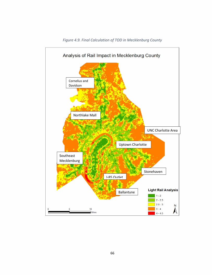
66  

Figure 4.9. Final Calculation of TOD in Mecklenburg County 

Uptown Charlotte 

UNC Charlotte Area

Northlake Mall 

Cornelius and 

Davidson 

Stonehaven 

Ballantyne

I‐85 Outlet

Southeast 

Mecklenburg 

 

67  

4.4 Index Value Interpretations

The reasons for developing this index value-based model for analyzing large scale

public transit improvements were detailed previously. Visualizing the distribution of

points along each of the maps is pivotal to being able to understand what the data say.

Highest positive intensity areas have low index values, while high negative intensity

areas have high index values. It can be seen in almost all of the maps that areas where

the Lynx light rail system serves have been changed dramatically over time. Since these

characteristics, i.e., land value and population, all have a high importance with respect to

city planning, it could be conjectured, and supported by evidence and research, that the

Lynx system had a large involvement in these changes over time.

Using this index model to identify and understand the changes associated with

Lynx or other systems, currently existing or planned for the future, by inputting values

associated with relevant variables can be done successfully. In this specific example,

using data collected from Mecklenburg County in North Carolina, an analysis of the

entire county, with a focus on the changes in variables around the Lynx LRT system, was

performed. Specific detailed interpretations are discussed subsequently, but it is

important to understand how to begin interpreting the results. As mentioned above, the

values are both visualized through maps and detailed in tables showing how changes over

time occurred in specific locations. By considering these results, it is possible to better

understand the possible relationships between the individual variables and the role that

the LRT system played.

 

68  

A legend is provided in each map, identifying the meanings behind the color

scheme and how they relate to the index values. In most cases, green colors are used to

represent negative changes, with other brighter colors generally representing positive

changes.

4.4.1 Emerging Transit-Oriented Development

With the calculation of existing TOD in areas surrounding the Lynx LRT, the

third objective for this research was to evaluate whether the model could be used to

determine locations where TOD may occur. It is apparent that with the data gathered

through this analysis, TOD in existing locations could be accurately determined. By

coupling these results with the planned route of the Northeast Extension of the LRT and

the same coding system, locations where potential for TOD to occur may be established

within a vicinity of the planned route.

The route was drawn according to the map provided by Mecklenburg County and

along the TIGER\line street files. Points where stations will be located along the route

were also placed in the map, including UNC Charlotte, which will be the Eastern

terminus of the line. These features were placed on top of the previously created image

alongside the existing LRT system to provide context and relevance for the possibility of

emerging TOD. What was shown by this comparison was an interesting display of

existing TOD already in the vicinity of UNC Charlotte, and a high propensity for future

growth trends in this direction.

With the plans for construction of the new line already underway, the first phase

of the project is already nearly completed. Unlike the first section, the new line will only

 

69  

partly overlap with existing freight rail, meaning that right-of-way acquisition will take

longer and be more costly. This likely means that the project will take longer

construction to begin and be completed so the time frame for the entire project will be

longer and be more ambiguous to analyze. The good news, as mentioned previously, is

that there already appears to be TOD in the works in the area near UNC Charlotte, so the

acquisition process may be more streamlined and take less time.

4.5 Assessment of Demographic Changes, Vehicle Ownership and Mode Split

4.5.1 Changes in Characteristics for Census Block Groups near Existing Rail Stations

As seen in Figure 4.10, there were some conflicting data points, namely personal

vehicle usage as a mode of primary transport decreased, but ownership of one or two

vehicles increased by owner and renter occupied delineations (renter denoted with a ‘2’ at

the end). One might expect that vehicle ownership would decrease as access to reliable

public transit increases over time (Chatman and Noland 2013), but this is not a

requirement, as evidenced by the data. It would appear that just because an individual

doesn’t need to drive a car as much does not mean that individual won’t continue to own

one or more vehicles. Positively, personal vehicle usage decreased dramatically over

time, with public transit consistently increasing to a minor degree. The percentage of

people walking more and reducing their car ownership to zero increased to a slight

degree, which is consistent with improved public transit. The factors most relevant in

this study, i.e., people using cars less and transit and non-motorized transport more, were

 

70  

present for Census BGs within 1.0 mile (1.6 km) of an existing rail station, again

exhibiting a positive trend with respect to the value of public transit.

 

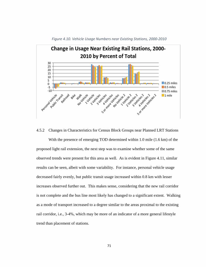
71  

Figure 4.10. Vehicle Usage Numbers near Existing Stations, 2000‐2010 

4.5.2 Changes in Characteristics for Census Block Groups near Planned LRT Stations

With the presence of emerging TOD determined within 1.0 mile (1.6 km) of the

proposed light rail extension, the next step was to examine whether some of the same

observed trends were present for this area as well. As is evident in Figure 4.11, similar

results can be seen, albeit with some variability. For instance, personal vehicle usage

decreased fairly evenly, but public transit usage increased within 0.8 km with lesser

increases observed further out. This makes sense, considering that the new rail corridor

is not complete and the bus line most likely has changed to a significant extent. Walking

as a mode of transport increased to a degree similar to the areas proximal to the existing

rail corridor, i.e., 3-4%, which may be more of an indicator of a more general lifestyle

trend than placement of stations.

 

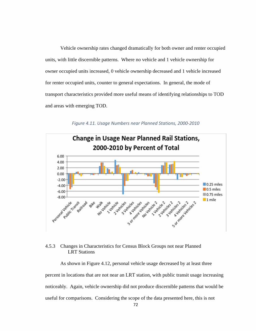
72  

Vehicle ownership rates changed dramatically for both owner and renter occupied

units, with little discernible patterns. Where no vehicle and 1 vehicle ownership for

owner occupied units increased, 0 vehicle ownership decreased and 1 vehicle increased

for renter occupied units, counter to general expectations. In general, the mode of

transport characteristics provided more useful means of identifying relationships to TOD

and areas with emerging TOD.

Figure 4.11. Usage Numbers near Planned Stations, 2000‐2010 

4.5.3 Changes in Characteristics for Census Block Groups not near Planned

LRT Stations

As shown in Figure 4.12, personal vehicle usage decreased by at least three

percent in locations that are not near an LRT station, with public transit usage increasing

noticeably. Again, vehicle ownership did not produce discernible patterns that would be

useful for comparisons. Considering the scope of the data presented here, this is not

 

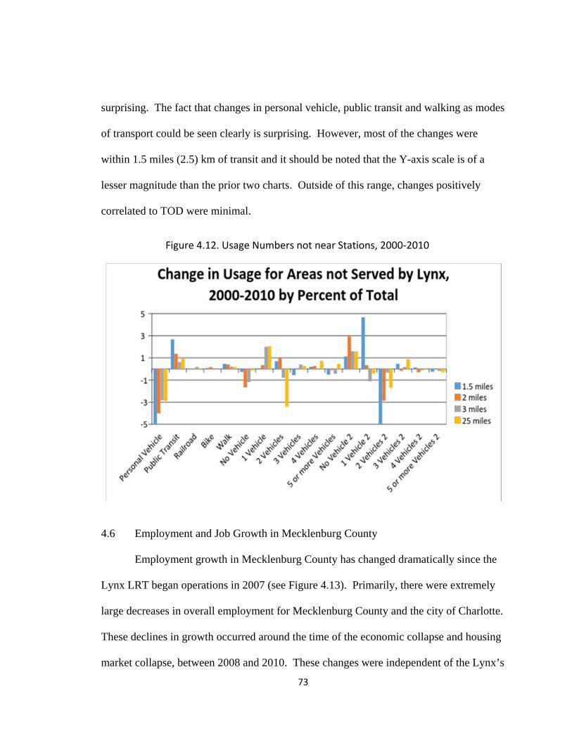
73  

surprising. The fact that changes in personal vehicle, public transit and walking as modes

of transport could be seen clearly is surprising. However, most of the changes were

within 1.5 miles (2.5) km of transit and it should be noted that the Y-axis scale is of a

lesser magnitude than the prior two charts. Outside of this range, changes positively

correlated to TOD were minimal.

 

  

4.6 Employment and Job Growth in Mecklenburg County

Employment growth in Mecklenburg County has changed dramatically since the

Lynx LRT began operations in 2007 (see Figure 4.13). Primarily, there were extremely

large decreases in overall employment for Mecklenburg County and the city of Charlotte.

These declines in growth occurred around the time of the economic collapse and housing

market collapse, between 2008 and 2010. These changes were independent of the Lynx’s

Figure 4.12. Usage Numbers not near Stations, 2000‐2010 

 

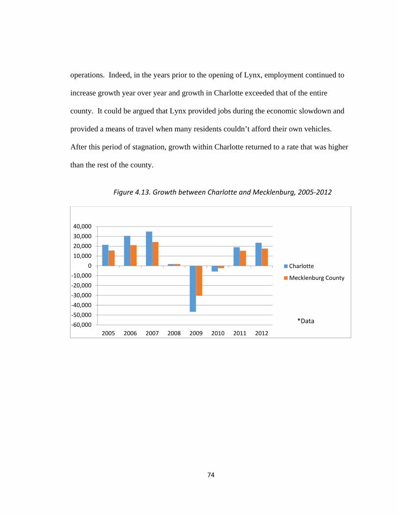
74  

operations. Indeed, in the years prior to the opening of Lynx, employment continued to

increase growth year over year and growth in Charlotte exceeded that of the entire

county. It could be argued that Lynx provided jobs during the economic slowdown and

provided a means of travel when many residents couldn’t afford their own vehicles.

After this period of stagnation, growth within Charlotte returned to a rate that was higher

than the rest of the county.

Figure 4.13. Growth between Charlotte and Mecklenburg, 2005‐2012

 

‐60,000

‐50,000

‐40,000

‐30,000

‐20,000

‐10,000

0

10,000

20,000

30,000

40,000

2005 2006 2007 2008 2009 2010 2011 2012

Charlotte

Mecklenburg County

*Data 

 

75  

CHAPTER V

CONCLUSIONS

5.1 Conclusions and Discussion

The purpose of this research was to identify specific key variables that are related

to transit oriented development (TOD) and develop a model that could combine them for

a comprehensive analysis that had not been done previously.

There were significant realizations with the individual analyses performed such as

the existence of overlap between population growth, housing unit density and peaks in

land value over time. They each showed considerable positive, TOD-trending changes

within close proximity, i.e., less than 1.0 miles (1.6 km) of northern stations on the Lynx

line, with other moderate changes along the rest of the line.

Specific variables provided more focused results that delineated critical locations

with relation to the Lynx LRT. Land value change and population change showed high

degrees of positive change within 0.4 miles (0.6 km) of a rail station, especially in the

area of Uptown Charlotte and the southern segment of the rail line. Along the middle

segment of the Lynx line, there were more ambiguous relationships between the variables

and the possibility of the presence of TOD, although there were minimal positive changes

in clusters that could be seen in the raster images. These were most obvious in the

analyses of land value and population change. In these two analyses, there were

 

76  

significant changes indicative of TOD on the eastern side of the rail line, primarily within

a mile of transit stations. Population growth was significant in this area, numbering in

the thousands in just one decade. The fact that this particular growth was localized, and

less than two miles (3.25 km) from a transit station was highly indicative of focused

growth, likely with relation to TOD.

5.2 Pre-Existing Limitations

There were limitations to some aspects of this research, the most obvious being a

lack of alternate case studies to use for comparison and/or validation. One of the primary

purposes of developing this GIS-based index with such a diverse amount of data, and

operating at as high a resolution as possible, was to provide a model that can be modified,

scaled and appended as desired. This model should be able to be applied to existing,

planned and potential corridors and localities where transit systems could be enhanced or

put into place. By working to include other comprehensive case studies from additional

systems, such as those focused on Denver, Florida, Seattle and San Francisco could serve

to significantly improve the accuracy and applicability of the model.

Additionally, there is a need for data that covers a longer time scale since 10 years

is a relatively short period in the life of a public transit system. For example, systems

like BART or other urban systems their impacts have been in effect for decades. In the

case of the Washington, DC Metro which is approximately 40 years old, it is also

undergoing a substantial expansion that could provide a good basis for additional study.

However, it needs to be remembered that a significant limitation is that of trying to get

 

77  

complete data over an extended period since many municipalities are inconsistent or

irregular in the manner and timing of tax parcel and similar data collection.

5.3 Future Directions

The model described in this thesis does not include all variables that could have

relevance in this line of research. Employment is a factor that likely has as high a

significance as those of land values and housing density in determining the value and

effectiveness of transit in new environments. Unfortunately, employment growth and

decline are not typically tracked at scales better than those associated with the county or

city level. For the model described in this thesis, all data involved needed to represent a

relatively small demographic, which the Bureau of labor Statistics did not have available.

Once this type of data becomes available, than employment will be a very powerful

variable to address in conjunction with land-related variables.

Additional factors that should be included, once there is evidential support, will

be variables such as property vacancy. This variable would be useful with relation to

crime statistics (again only as it pertains to relatively small amounts of people, such as at

the Block Group level). Following along the lines of the “Broken Windows Theory,” the

more locations are vacant, damaged, etc., the higher will be the, mostly non-violent,

crime rates (Wilson and Kelling , 1982).

If transit systems can bring people, jobs and increased values to specific locations

that have previously had little or none, than it could be surmised that a positive

correlation exists between all of these factors and TOD. The viability of a further

evaluation of these and other aspects of urban/suburban development related to healthy

 

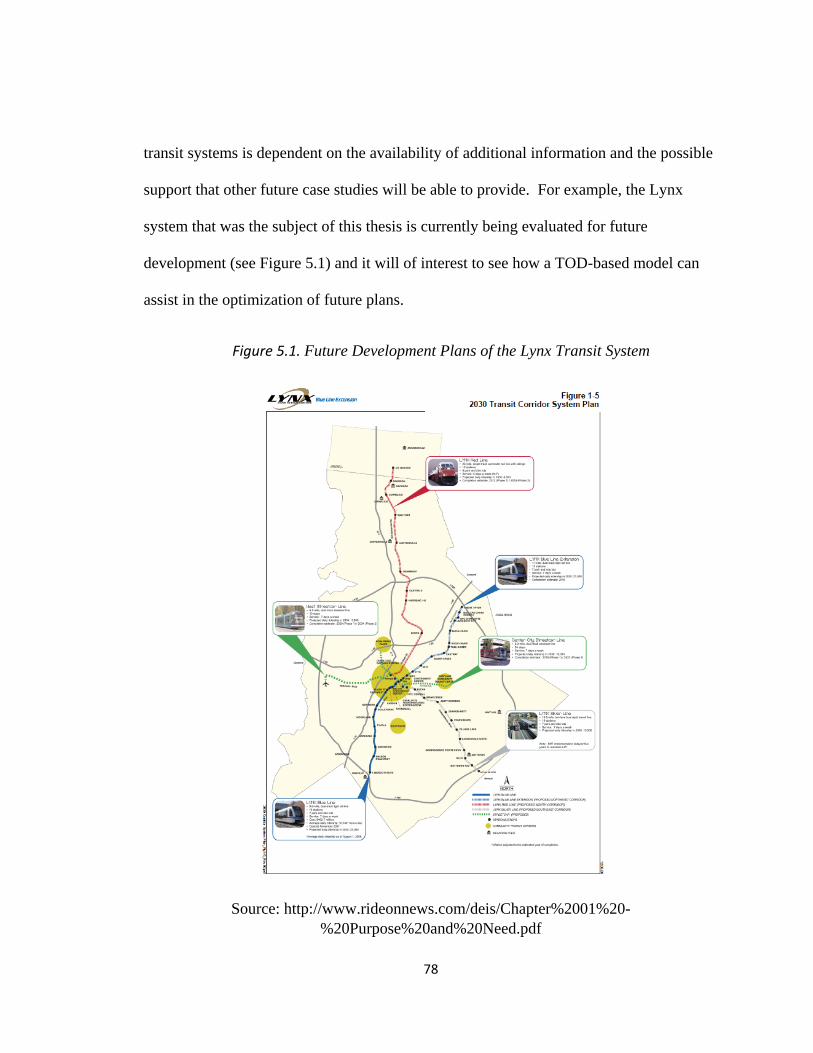
78  

transit systems is dependent on the availability of additional information and the possible

support that other future case studies will be able to provide. For example, the Lynx

system that was the subject of this thesis is currently being evaluated for future

development (see Figure 5.1) and it will of interest to see how a TOD-based model can

assist in the optimization of future plans.

Source: http://www.rideonnews.com/deis/Chapter%2001%20-%20Purpose%20and%20Need.pdf

Figure 5.1. Future Development Plans of the Lynx Transit System

 

79  

REFERENCES

Al-Dubikhi, Sami, and Paul Mees. "Bus Rapid Transit in Ottawa, 1978 to 2008:

Assessing the Results."Town Planning Review, 2010, 407-24.

Augustin-Jean, Louis. "Urban Planning In Hong Kong and Integration with the Pearl

River Delta: A Historical Account of Local Development." GeoJournal 62, no. 1-

2 (2005): 1-13.

Bailey, Keiron, Ted Grossardt, and Michaele Pride-Wells. "Community Design of a Light

Rail Transit-oriented Development Using Casewise Visual Evaluation

(CAVE)." Socio-Economic Planning Sciences, 2007, 235-54.

Batt, H. William. "Value Capture as a Policy Tool in Transportation Economics: An

Exploration in Public Finance in the Tradition of Henry George." American

Journal of Economics and Sociology, 2001, 195-228.

Baum-Snow, Nathaniel, and Matthew E. Kahn. "Effects of Urban Rail Transit

Expansions: Evidence from Sixteen Cities, 1970-2000."Brookings-Wharton

Papers on Urban Affairs, 2005, 147-206.

Baumel, C. Phillip, John J. Miller, and Thomas P. Drinka. "The Economics of Upgrading

Seventy-One Branch Rail Lines in Iowa." American Journal of Agricultural

Economics, 1976, 61.

Brown, B. B., and C. M. Werner. "The Residents' Benefits and Concerns Before and

After a New Rail Stop: Do Residents Get What They Expect?" Environment and

Behavior, 2010, 789-806.

Cervero, Robert. "Growing Smart by Linking Transportation and Land Use: Perspectives

from California." Built Environment, 2003, 66-78.

Cervero, R. "Transport Infrastructure and Global Competitiveness: Balancing Mobility

and Livability."The Annals of the American Academy of Political and Social

Science, 2009, 210-25.

 

80  

Cervero, Robert, and Michael Duncan. "Transit's Value-Added Effects: Light and

Commuter Rail Services and Commercial Land Values." Transportation Research

Record, 2002, 8-15.

Cervero, Robert, and John Landis. "Twenty Years of the Bay Area Rapid Transit System:

Land Use and Development Impacts,"Transportation Research Part A: Policy

and Practice 31, no. 4 (1997): 309-33.

Chakraborty, Arnab, and Sabyasachee Mishra. "Land Use and Transit Ridership

Connections: Implications for State-level Planning Agencies." Land Use Policy,

2012, 458-69.

Chatman, Daniel G. "Does TOD Need the T?" Journal of the American Planning

Association, 2013, 17-31.

Chiang, Wen-Chyuan, Robert A Russell, and Timothy L Urban. "Forecasting Ridership

for a Metropolitan Transit Authority.” Transportation Research Part A: Policy

and Practice, 2011, 696-705.

Dejong, T. M. "A Comparison of Three Diversity Indices Based on Their Components of

Richness and Evenness."Oikos 26.2 (1975): 222. Print.

Dorsey, Bryan, and Alice Mulder. "Planning, Place-making and Building Consensus for

Transit-oriented Development: Ogden, Utah Case Study." Journal of Transport

Geography, 2013, 65-76.

Forrest, David, John Glen, and Robert Ward. "The Impact of a Light Rail System on the

Structure of House Prices. "Journal of Transport Economics and Policy (1996):

15-29. JSTOR.Web. 13 Jan. 2014.

Geller, A. L. "Smart Growth: A Prescription for Livable Cities." American Journal of

Public Health, 2003, 1410-415.

Gihring, Thomas A. "Applying Value Capture in the Seattle Region." Planning Practice

and Research, Summer 1991, 307-20.

Goldberg, Michael. "Transportation, Urban Land Values, and Rents: A Synthesis." Social

Research 46, no. 2 (1970): 153-62.

 

81  

Haig, Robert Murray and McCrea, Roswell C. “1876-1951, Major economic factors in

metropolitan growth and arrangement: a study of trends and tendencies in the

economic activities within the region of New York and its environs.” Arno Press,

New York, 1974.

Horner, Mark W., and Daniel Schleith. "Analyzing Temporal Changes in Land-use–

transportation Relationships: A LEHD-based Approach." Applied Geography,

2012, 491-98.

Hubbell, John, and Dave Colquhoun. "Light Rail Transit in Calgary: The First 25 Years."

Joint International Light Rail Conference, 2006.

Katz, Bruce, and Amy Liu."Moving Beyond Sprawl toward a Broader Metropolitan

Agenda,"The Brookings Review 18.2 (2000): 31-34. JSTOR.Web.

Kay, Andrew, Robert Noland, and Stephanie DiPetrillo. "Residential Property Valuations

Near Transit Stations with Transit-Oriented Development."Journal of Transport

Geography 39 (2014): 131–140.

Kim, Jin. "Disciminant Impact of Transit Station Location on Office Rent and Land

Value in Seoul." Journal of Transport Economics and Policy 41, no. 2 (2007):

219-45.

Koutsopoulos, K. C. "The Impact of Mass Transit on Residential-Property Values."

Annals of the Association of American Geographers 67.4 (1977): 564-76. Print.

Lundberg, Benjamin, and Joseph Weber. "Non-motorized Transport and University

Populations:

An Analysis of Connectivity and Network Perceptions."Journal of Transport

Geography 39 (2014): 165–178.

Maurer, Lindsay. "Suitability Study for a Bicycle Sharing Program in Sacramento,

California,"2011, 1-43.

Mohan, Dinesh. "Mythologies, Metro Rail Systems and Future Urban

Transport." Economic and Political Weekly 43, no. 4 (2008): 41-53.

 

82  

Novak, David C., James L. Sullivan, and Darren M. Scott. "A Network-based Approach

for Evaluating and Ranking Transportation Roadway Projects."Applied

Geography, 2012, 498-506.

Parry, Ian W. H, and Kenneth A Small. "Should Urban Transit Subsidies Be Reduced?"

American Economic Review 99, no. 3 (2009): 700-24.

Perry, James L., and Timlynn T. Babitsky. "Comparative Performance in Urban Bus

Transit: Assessing Privatization Strategies."Public Administration Review, 1986,

57.

Ravibabu, M. "Viability of Surface Rail for Urban Mass Transit." Economic and Political

Weekly, 2006, 1506.

Ross, Catherine L. "Policy & Practice: Transport and Megaregions: High-speed Rail in

the United States." Town Planning Review, 2011, 341-56.

Sherali, Hanif D., ChawalitJeenanunta, and Antoine G. Hobeika. "The Approach-

dependent, Time-dependent, Label-constrained Shortest Path Problem."Networks,

2003, 57-67.

Smit, Han T.J., and Lenos Trigeorgis. "Valuing Infrastructure Investment: An Option

Games Approach."California Management Review, 2009, 79-100.

Smith, Jeffery J., and Thomas A. Gihring. "Financing Transit Systems through Value

Capture," American Journal of Economics and Sociology, 2006, 751-86.

Smith, Robert. "Reorganization of Regional Transportation Authorities to Maintain

Urban/Suburban Constituency Balance."Public Administration Review 47, no. 2

(1987): 171-79.

Topalovic, P., J. Carter, M. Topalovic, and G. Krantzberg. "Light Rail Transit in

Hamilton:

Health, Environmental and Economic Impact Analysis." Social Indicators

Research 108, no. 2 (2012): 329-50.

University of Washington."Seattle Bicycle Share Feasibility Study."American Planning

Association, 2010, 1-123.

 

83  

Wilson, J. Q, and Kelling, G. L., Broken Windows: The police and neighborhood safety,

The Atlantic, March, 1982.

Wirasinghe, S. Chandana, Vanolin F. Hurdle, and Gordon F. Newell. "Optimal

Parameters for a Coordinated Rail and Bus Transit System." Transportation

Science 11, no. 4 (1977): 359-74.

Woodbury, Coleman. "Transit and the Trend of Multi-Family Housing."Journal of Land

&Public Utility Economics 7, no. 1 (1931): 36-44.

Wunsch, Pierrre. "Cost and Productivity of Major Urban Transit Systems in

Europe."Journal of Transport Economics and Policy 30, no. 2 (1996): 171-86.