Embed Size (px)
Citation preview

Final Report
April 2015
Decentralized
Coordination
Procedures
MicroGrids


Smart Nord
Final Report
Editors:
Prof. Dr.-Ing. habil. Lutz Hofmann
and
Prof. Dr. rer. nat. habil. Michael Sonnenschein
The Lower Saxony research network “Smart Nord” acknowledges the support of the Lower
Saxony Ministry of Science and Culture through the “Niedersächsisches Vorab” grant
programme (grant ZN2764/ZN 2896).
Hanover, April 2015
Please cite the contributions to this report in the following manner:
Author(s), “Full Title of the Work Package or Full Title of the Sub-Project,” in L. Hofmann and
M. Sonnenschein, “Smart Nord - Final Report”, pp. #-#, Hanover, April 2015.
ISBN: 978-3-00-048757-6
Printed by: Druckerei Hartmann GmbH, Hannover


Preface
5
Preface
The Lower Saxony research network “Smart Nord” has achieved its goals. In this research network
supported by Lower Saxony’s Ministry of Science and Culture through the “Niedersächsisches
Vorab” grant programme with an amount of 4.1 Million €, about 40 scientists of the universities of
Oldenburg, Brunswick, Hanover and Clausthal as well as the OFFIS Institute for Information
Technology, the Energy Research Centre of Lower Saxony and NEXT ENERGY, the EWE-
Research Center of Energy Technology e. V. worked together for three years in six sub-projects.
In the past three years (from 3/2012 to 2/2015) the interdisciplinary research network Smart Nord
aimed to create contributions to coordinated, decentralized provision of active power, control
power and reactive power in distribution grids which allow a stable system operation. Therefore,
the development of a new ICT infrastructure which includes all the new components of the
distribution grids is required.
The sub-projects were motivated by the transformation of the European and especially German
power system which includes the shutdown of nuclear power plants, the replacement of fossil
power plants with converter based decentralized generation units, the ever intensifying European
power market and installation of Smart Grids and their ICT infrastructure. In addition to these
changes, a high amount of new power lines and transformers to fulfil the changing transmission
and distribution tasks will be included in all grid voltage levels as well as new control strategies.
Based on this transformation of the power system, sub-project (SP) 1 was focused on methods for
decentralized coordinated active power management to allow decentralized and especially
renewable generation units to contribute to the power market. Another market which can be opened
to these units is the market for ancillary services, especially provision of control power and reactive
power, to support the power grid and the realization of the technical requirements (SP 2). The
design and requirements of these above mentioned future markets had to be set within the project
(SP 3). This included the design of new products and marketing opportunities. Based on the unit
dispatch which resulted from SP 1-3, the resulting states of the transmission and distribution grids
were evaluated in stationary and dynamic simulations to analyse the frequency stability in order to
identify measures to ensure frequency stability in future grids (SP 4). The control strategies for
distribution grids with a high amount of volatile converter connected generation units were also
evaluated (SP 5). This included strategies for distribution grids connected to the transmission grid
and islanding distribution grids without connection to other grids. SP 6 aimed at the analysis of the
potential for the construction of new renewable generation units based on environmental
conditions.
The following report introduces Smart Nord to you and shows the various results of the sub-
projects and their work packages. For further information please visit www.smartnord.de.
Prof. Dr.-Ing. habil. Lutz Hofmann Prof. Dr. rer. nat. habil. Michael Sonnenschein
Institute of Electric Power Systems Department of Computing Science
Leibniz Universität Hannover Carl von Ossietzky Universität Oldenburg


Table of Contents
7
Table of Contents
Introduction .................................................................................................................................... 11
Smart Nord ................................................................................................................................ 13
Overview on Smart Nord .......................................................................................................... 15
Work Group: Scenario Design for Sub-Projects 1-4 .................................................................. 19
Work Group: Scenario Design .................................................................................................. 21
Sub-Project One: Decentralized Provision of Active Power ...................................................... 33
Overview on Sub-Project One: Decentralized Provision of Active Power ............................... 35
Work Package 1.1: Use of Electrical Energy Storages to Support a Schedule-Based Energy
Management .............................................................................................................................. 43
Work Package 1.2: Decentralized Active Power Provision ...................................................... 51
Work Package 1.3: Optimization of Cluster Schedules ............................................................ 59
Work Package 1.4: Continuous Scheduling .............................................................................. 69
Work Package 1.5: Information Security in Agent-Based Energy Management Systems ....... 77
Sub-Project Two: Grid Stabilizing Ancillary Services ............................................................... 93
Overview on Sub-Project Two: Grid Stabilizing Ancillary Services ....................................... 95
Work Package 2.1: Coordinated Coalitions for Real-time Provision of Ancillary Services .... 97
Work Package 2.2: Reliable Contribution Planning and Risk Management of Coordinated
Coalitions for the Provision of Ancillary Services ................................................................. 105
Work Package 2.3: Interoperability and Performance Issues of Coalition Formation for
Ancillary Services ................................................................................................................... 113
Work Package 2.4: Small-Signal Stability of Frequency-Response Coalitions ...................... 119
Work Package 2.5: Grid-Supporting Services Through Inverters .......................................... 127
Sub-Project Three: Integrated Market ...................................................................................... 139
Overview on Sub-Project Three: Integrated Market ............................................................... 141
Work Package 3.1: Analysis and Development of Prospective System Services ................... 143
Work Package 3.2: Market Design ......................................................................................... 149
Work Package 3.3: Business Models for Energy Producer and Price Sensitive Consumer.... 157
Sub-Project Four: Distribution and Transmission System ...................................................... 165
Overview on Sub-Project Four: Distribution and Transmission System ................................ 167
Work Package 4.1: Interconnected System ............................................................................. 169
Work Package 4.2: Low-Voltage Grid Modelling and Grid Compatibility Assessment ........ 185

Smart Nord Final Report
8
Sub-Project Five: System Theory for Active Distribution Grids ............................................. 197
Overview on Sub-Project Five: System Theory for Active Distribution Grids ...................... 199
Work Package 5.1: System Theory for MicroGrids ................................................................ 201
Work Package 5.2: System Theory of Generation and Loads ................................................ 213
Work Package 5.3: Demonstration Plant for MicroGrids under Consideration of Islanding
Detection ................................................................................................................................. 221
Sub-Project Six: SmartSpatial .................................................................................................... 233
SmartSpatial ............................................................................................................................ 235
Annex ............................................................................................................................................. 261
List of Publications Written in Smart Nord ............................................................................ 263
List of Doctoral Theses ........................................................................................................... 271


Introduction
11
Introduction


Introduction
13
Smart Nord
“Smart Nord – Intelligente Netze Norddeutschland” which stands for “smart grids in northern
Germany” is an interdisciplinary research network supported for three years (from 3/2012 to
2/2015) by the Lower Saxony Ministry of Science and Culture through the “Niedersächsisches
Vorab” grant programme with 4.1 Million €. Smart Nord was organized in six sup-projects with
research partners from up to four universities and research institutes which were:
Sub-Project One - Decentralized Provision of Active Power
coordinated by Michael Sonnenschein
Research partners:
University of Oldenburg
OFFIS – Institute for Information Technology
Technische Universität Braunschweig
Sub-Project Two - Grid Stabilizing Ancillary Services
coordinated by Sebastian Lehnhoff
Research partners:
OFFIS – Institute for Information Technology
University of Oldenburg
Leibniz Universität Hannover
Technische Universität Braunschweig
Sub-Project Three - Integrated Market
coordinated by Michael Kurrat
Research partners:
Technische Universität Braunschweig
OFFIS – Institute for Information Technology
Leibniz Universität Hannover
Sub-Project Four - Distribution and Transmission System
coordinated by Lutz Hofmann
Research partners:
Leibniz Universität Hannover
Technische Universität Braunschweig
EWE-Forschungszentrum für Energietechnologie e.V.
Sub-Project Five - System Theory for Active Distribution Grids
coordinated by Hans-Peter Beck
Research partners:
Clausthal University of Technology
University of Oldenburg

Smart Nord Final Report
14
Sub-Project Six – SmartSpatial
coordinated by Christina von Haaren
Research partners:
Leibniz Universität Hannover
On the following pages an overview over the research aims of the six sub-projects is given. They
are introduced with a brief explanation and visualisation of the contents as well as their interaction
and collaboration, especially in the sub-projects 1-4 within the work group scenario design.

Introduction
15
Overview on Smart Nord
The following pictures and annotations shall give a general overview and understanding of the
connections and collaborations between the system layers market, function, information, hardware,
grid and environment, which are handled in the sub-projects 1-6 and the collaborations between the
sub-projects.
Figure 1 shows the setup and connections of the sub-projects 1-4. The main research areas of these
sub-projects are the operation of an interconnected energy system spreading over four voltage
levels with a high amount of decentralized renewable generation. In the SP new decentralised
market structures are examined in addition to a market based interface. A necessary part of the
market is the market for ancillary services which is based on so far existing units. In the lower
voltage levels of the distribution grid, the units are organised within virtual dynamic coalitions.
These coalitions are subjected to a decentralized regulation and control strategy which is realized
by an agent-based information and communication technology (ICT) infrastructure.
Market for Ancillary Services
German Market for Energy
European Market for Energy
Info
rma
tio
nH
ard
wa
reS
up
ply
Fu
nct
ion
Ma
rke
t
Tra
nsm
issi
on
Sm
art
Sp
ati
al
Autonomous System Local Services
Figure 1: Setup and connections of sub-projects 1-4

Smart Nord Final Report
16
Based on the design of new tradable products and the results of the markets, further analysis is
possible. The stationary operational behaviour of the system under the constraints of decentralised
provision of active and reactive power as well is calculated for several stationary cases and
evaluated with regard to operational and technical boundary conditions. In addition to stationary
analysis, the decentralised provision of ancillary services to ensure the frequency stability and
measures to ensure the frequency stability in future systems are analysed.
In order to work together on comprehensive topics, specialised work groups were established. The
work group Scenario Design has developed joint scenarios and herewith corresponding grid models
as joint evaluation environment for the studies in sub-projects 1-4 to allow a common simulation at
several research institutes and an exchange of research results.
Market for Ancillary Services
German Market for Energy
European Market for Energy
Info
rma
tio
nH
ard
wa
reS
up
ply
Fu
nct
ion
Ma
rke
t
Tra
nsm
issi
on
Sm
art
Sp
ati
al
Autonomous System Local Services
Figure 2: Setup of SP 5

Introduction
17
Figure 2 shows the setup of SP 5 and possible connections to the other SP. Within this SP,
MicroGrids with a high amount of renewable generation units are evaluated. These MicroGrids are
simulated as islanded grids without any connections to neighbour grids and as part of the
interconnected energy system. In addition, the possibilities of a virtual synchronous generator for
providing ancillary services with the use of converters are evaluated. The second part of this SP is a
system-theoretical approach influenced by the stochastic disturbance of regenerative systems. The
last part of this SP is the construction of a demonstrator to evaluate the simulations in real power
systems.
Figure 3 shows the setup of SP 6. This SP evaluated the local potential of possible construction
sites for renewable generation units. It identifies the potential of several renewable energy sources
in predesigned regions and identifies an efficient energy mix for a specific region under
consideration of environmental requirements.
Market for Ancillary Services
German Market for Energy
European Market for Energy
Info
rma
tio
nH
ard
wa
reS
up
ply
Fu
nct
ion
Ma
rke
t
Tra
nsm
issi
on
Sm
art
Sp
ati
al
Autonomous System Local Services
Figure 3: Setup of SP 6
On the following pages detailed reports of each SP are given. These detailed reports are headed by
an introduction of the joint evaluation scenarios which were created by the work group scenario
design for the sub-projects 1-4.


Scenario Design for Sub-Projects 1-4
19
Work Group:
Scenario Design for Sub-Projects 1-4


Scenario Design for Sub-Projects 1-4
21
Work Group: Scenario Design
Marita Blank1, Timo Breithaupt
2, Jörg Bremer
1, Arne Dammasch
3, Steffen Garske
2,
Thole Klingenberg4, Stefanie Koch
3, Ontje Lünsdorf
4, Astrid Nieße
4, Stefan Scherfke
4,
Lutz Hofmann2 and Michael Sonnenschein
1
1 Goals
Within the multi-disciplinary research project Smart Nord, different research questions have been
addressed which concern different fields and system levels. However, several work packages
require cross-disciplinary information and models and are dependent on results from other project
partners. A simulation of the whole system taking into account all research questions within all
work packages was not available and could not be realised at once. Nevertheless, the evaluation of
the SP 1-4 had to be built on the same basic assumptions in order to guarantee compatible and
comparable project results. For this reason, the work group Scenario Design – consisting of
researchers from all partner institutes and work packages – has developed joint scenarios and
herewith corresponding grid models as evaluation environment for all partners in the SP 1-4.
The scenarios had to be valid for all voltage levels from ultra-high voltage to low voltage and have
been transferred to the corresponding grid models. Furthermore, the present regional structure of
loads and generating units had to be represented as well as estimations for their future development
according to actual studies (see Section 3). With the developed scenarios characteristic points in
time (high load, low load) and time horizons (e.g. winter, summer) can be investigated in order to
evaluate the different algorithms und approaches within the project under different case studies.
2 Related Work
The terms scenario and scenario design are used in different ways depending on the domain under
investigation [1] (e.g. in companies, energy system, algorithm design) and the purpose the
scenarios are used for. In companies, scenarios for future development can be used to identify new
business strategies [2]. For energy systems, the design of future scenarios is an essential step for
research studies. There, scenarios are used, e.g., to define goals for future energy systems (e.g. the
energy concept of Germany [3]) or to make assumptions or predictions on future developments of
the overall energy system. The predictions can be utilised to evaluate the development of different
system parameters such as the need for network expansion depending on, e.g., different energy
mixes or different assumption on energy consumption ([4], [5], [6] and [7]). Moreover, structural
and economic effects can be investigated for different scenarios and conclusions can be drawn for
different approaches such as the need of flexibility (e.g. [8]). In [9] migration paths are described
for information and communication technologies of different Smart Grid scenarios. Furthermore,
scenario design is an important step during algorithm engineering especially for applications in
Smart Grid approaches [10].
1 University of Oldenburg, 26129 Oldenburg, Germany,
[email protected], Department of Computing Science 2 Leibniz Universität Hannover, 30167 Hanover, Germany,
[email protected], Institute of Electric Power Systems (IEH) 3 Technische Universität Braunschweig, 28106 Braunschweig, Germany,
first [email protected], elenia 4 OFFIS – Institute for Information Technology, 26121 Oldenburg, Germany,
[email protected], R&D Division Energy

Smart Nord Final Report
22
However, a uniform or standardised process for scenario design does not exist [1]. The vast amount
of scenarios and their different usage shows that the design of scenarios strongly depends on the
purpose and investigations to be conducted.
3 Methodology
For the development of the scenarios within this research project as a first step, the work group
Scenario Design collected requirements from the different work packages to ensure that the
scenarios are suitable for the investigations of all work packages. Two main scenarios - a reference
scenario 2011 and a future outlook of the year 2030 - have been aligned. Based on these
requirements a process has been developed to define and realise the scenarios in the available
evaluation environments in all SP. This process is visualised in Figure 1.
First, the Basic Assumptions (4.1) were made on which the scenarios were built. These include all
basic information as grid, load and generation data for as well the reference year 2011 as the future
outlook of the year 2030. The assumptions are mainly based on the governmental plans for the
transformation of the energy supply system and furthermore the corresponding studies regarding
grid expansion in transmission and distribution grids (Section 4.1). Furthermore, requirements from
the simulation environments available and used at each SP have been identified which were
necessary to adapt to the scenario requirements and to obtain an overall coherent simulation
environment. Thus as the second step, the transmission grid model used in the work package 4.1
has been determined in order to define coupling points to underlying grid levels (see Section 4.2
Top-Down). As a third step, requirements from the distribution grid have led to defining coupling
points to the higher voltage levels (see Section 4.3 Bottom-Up). In a fourth step, the unit
distribution within the distribution grid has been computed in order to represent the actual and
regional structure of load and generation. Hence the according units have been distributed and
connected to the grid model nodes followed by a validation and verification of the grid
compatibility of these generated grid models (cf. work package 4.2).
MV
MV
MV
MV MV
MV
MV
MV
MV
MV
MV
MV
MV
MV
UHV –Ultra-high voltage
HV –High voltage
MV –Medium voltage
LV –Low voltage
1Basic
Assumptions
Reference year 2011
Future outlook 2030
2 Top-DownModeling of high-voltage grids
Definition of coupling points at MV nodes
Load- and generation models (HV - MV)
3 Bottom-UpModeling of MV and LV-grids
Distribution of MV- and LV-grids
Load- and generation models (MV - LV)
4Unit
Distribution
Distribution of units to MV- and LV-nodes
(generators, consumers, storages)
Validation and grid compatibility
Figure 1: Process for scenario definition

Scenario Design for Sub-Projects 1-4
23
In both analyses – the top-down and bottom-up step – requirements and data interfaces for load and
generating units were identified that comply with the assumptions and coupling points. The results
of this process are coherent grid models for both distribution and transmission grid within this
research project with corresponding load and generation distribution for both scenarios (2011 and
2030).
4 Main Results
As the process itself is a main result of the work group, the individual steps of the process
introduced in the previous section of this chapter are being presented in more detail. Furthermore
excerpts of the results and realisation of the scenarios are shown as well. For more detailed
descriptions refer to the corresponding work packages and further [11] and [12].
4.1 Basic Assumptions
The Basic Assumptions form the foundation for the scenarios, since they establish the scope for
investigations of the SP 1-4. The steps 2-3 (Figure 1) are the realisation of the scenarios in order to
obtain a setting and environment to conduct experimental evaluations.
For investigations of a segment of the distribution grid, the structure of loads and distributed
generating (DG) units for rural grids were chosen to represent the structure of rural regions in
Lower Saxony. To this end, statistical data of population of rural regions was utilised [13]. In order
to reflect the installed capacity in Lower Saxony according to the different voltage levels, the asset
master data of all installed renewable energy sources (RES) in the German transmission grid
operators [14] has been filtered. The joint reference year has been chosen to be 2011, whereas the
future horizon was specified to be the year 2030 because for this horizon a good basis of data and
studies were at hand. Predictions of growth of renewable and distributed energy resources as well
as assumptions on grid expansion had to be consistent throughout all voltage levels. The following
studies have been chosen to build the assumptions on 2030: BMU5 Long-term scenarios 2011 [8],
Netzentwicklungsplan 2012 [15], ENTSO-E6 Ten Years Network Development Plan (TYNDP) [6],
ENTSO-E Scenario Outlook & Adequacy Forecasts (SOAF) [7], Dena7 Verteilnetzstudie [4], and
BMWi8 Verteilernetzstudie [5].
4.2 Top-Down
The approach of the top-down step is based on an integrated grid and market simulation developed
in MATLAB9 by the IEH (refer to [11], [16] and [17]) which is used for simulations of the
European transmission system in this research project (cf. work package 4.1). The integrated
simulation is based upon several databases like e.g. measured load data of the ENTSO-E, a grid
model of the ENTSO-E interconnected continental transmission grid, generation data of all power
plants with an installed capacity greater than 50 MW and further generation as well as RES and DG
generation (all units smaller than 50 MW) as regional aggregated data [11], [10], [17]. The first
result of the simulation is an energy market simulation based on a merit order of marginal
costs (see work package 4.1). The according power plant dispatch is the input value for the load
flow calculations of the transmission system.
5 Bundesministerium für Umwelt, Naturschutz, Bau und Reaktorsicherheit (Federal Ministry for the
Environment, Nature Conservation, Building and Nuclear Safety), http://www.bmub.bund.de/en/ 6 European Network of Transmission System Operators for Electricity, https://www.entsoe.eu
7 Deutsche Energie-Agentur (German Energy Agency), www.dena.de/en/
8 Bundesministerium für Wirtschaft und Energie (Federal Ministry for Economic Affairs and Energy),
www.bmwi.de/EN/ 9 http://www.mathworks.com

Smart Nord Final Report
24
In this simulation environment the assumptions of the future outlook scenario 2030 have been
implemented into the generation data with the 2011 scenario as the existing reference scenario (see
Figure 3 as an example for the German transmission system model).
Scenario 2011 Scenario 2030
Figure 2: The scenarios 2011 and 2030 in the generation data for the
transmission system model
The forward projection of the power generation is based on the power plant database of the grid
and market model (see work package 4.1) and the Vision 3 of the SOAF [7]. The forecast in the
SOAF gives only information about the installed capacities of the different energy sources. Hence
different concepts for the distribution of the various types have been developed within this research
project to calculate the shares and the geographical allocation of each generation type within the
simulation model (see Figure 3).
Scenario 2011 Scenario 2030
solar
wind
hydro
further
oil & gas
hard coal
lignite
nuclear
Figure 3: The scenarios 2011 and 2030 in the generation allocation data for the
transmission system model
For biomass, garbage and not clearly identifiable energy sources all characteristics of the single
power plants listed remain the same except the nominal power. To estimate the nominal power for
every power station a scaling factor is calculated in relation of the target value (SOAF) and the sum
0
20
40
60
80
100
inst
alle
d p
ow
er i
n G
W
0
20
40
60
80
100
inst
alle
d p
ow
er i
n G
W

Scenario Design for Sub-Projects 1-4
25
of the nominal power listed in the database. Wind and solar power plants are scaled with the target
values and the geographical allocation of the power plants remains unchanged. Thermal power
plants and hydropower plants are first analysed regarding their expected lifetime within the
database [18], [19], [20]. Power plants whose lifetime ends before 2030 are removed. If the
remaining cumulative capacity is greater than the target value, the power plants starting with the
oldest are removed until the target value is reached. If the cumulative capacity is smaller than the
target value, new power plants are built in the second step using a trend line with consideration of
the average relative deviation for nominal power and efficiency at the same location. The trend
lines and the average relative deviations are estimated from existing and planned power plants [21].
As the nominal power of run-of-the-river power plants and storage power plants is strongly
influenced by the local conditions, the nominal power remains the same when these power plants
are rebuilt. Due to the small amount of heavy oil-fuelled power plants the identification of a trend
line is not possible. If the cumulative capacity is still smaller than the target value the missing
capacity needs to be added manually.
Within each scenario load flow calculations can be analysed for various characteristic points in
time. As the simulation model is based on the reference scenario 2011, the new generation
allocation (see Figure 3), which is based on the stated studies and the described allocation
algorithm, is not compatible with the present grid data. The extensive transformation of the
European energy supply system leads to a high need of grid expansion (compare [6], [15]). Thus
this required grid expansion according to the stated studies, including the high-voltage direct
current (HVDC) lines within the German transmission system (see Figure 4), had to be
implemented in the simulation model. Furthermore, because of divergences of the simulation
model and the stated studies, further grid expansions within the transmission grid model have been
implemented.
Scenario 2011 Scenario 2030
Ur = 380 kV
Ur = 220 kV
HVDC
Figure 4: The scenarios 2011 and 2030 in the transmission system model including the NEP 2012
One main research question of the project Smart Nord is the provision of active, reactive and
control reserve by dynamic virtual power plants (DVPP) in the underlying voltage levels to the
transmission system. Hence the distribution grid had to be implemented into the existing
transmission system model. This was realised with the stated top-down and bottom-up approach in
addition with distributed load and generation data models. On selected UHV nodes the existing
load and RES data was substituted with distributed HV and MV load and DG models in one

Smart Nord Final Report
26
distribution grid section model (see Figure 1). Therefrom, the top-down requirements for the
bottom-up coupling points are defined. The distribution section from HV to MV is based on
synthetic grids for the HV-level and a modification of a common MV-Benchmark
grid [22] (see 4.3). With the distribution grid sections coupled to the transmission system with
individual load and RES data for each node, both scenarios can be evaluated in an integrated
transmission and distribution system model [12].
4.3 Bottom-Up
Within the project, data of rural LV grids have been available from which realistic grid parameters
were identified such as data of transformers, number of house connection nodes, line lengths and
line types. This data was the basis for modelling eight LV-grids with typical rural grid structures.
For completion, household profiles were generated (cf. [23]). To this end, different domestic
consumers were modelled depending on size of households and technical equipment, e.g. how
domestic warm water is prepared. The resulting profiles of domestic consumption for one year
were validated by checking the correlations with the standardised load profile H0 from BDEW10
.
For simplification, commerce and industry were neglected within the MV and LV level.
As a model for an MV-grid a sub-network of the Cigre-Benchmark Grid [22] was chosen and
adapted according to the requirements of the research project. According to Figure 5 the sub-
network I has been used for evaluations in Smart Nord. The LV model-grids have been randomly
connected to the MV-nodes according to the maximum load at the MV/LV-transformers and
furthermore the specification of maximum power at the coupling point (HV/MV) from the top-
down step. For modelling the scenario grids of the distribution level, the software DIgSILENT
PowerFactory11
was used. Due to the many opportunities and the high adaptability of the software,
the lower voltage levels (LV, MV) were completely simulated using PowerFactory within the work
package 4.2 and further as one part of the top-down step in the transmission system model (work
package 4.1) in the MATLAB simulation.
10
Bundesverband der Energie- und Wasserwirtschaft e.V. (Federal Association of the Energy and Water
Industry), https://www.bdew.de/ 11
PowerFactory is a professional network calculation tool, which can be adjusted via freely programmable
scripts (DPL Programming Language). The program is also capable of calculating very large power grids.
Far from the modeling PowerFactory includes all common analysis tools such as load flow, short-circuit,
harmonic calculations, contingency calculation and reliability analysis.

Scenario Design for Sub-Projects 1-4
27
Figure 5: Graph of a German medium-voltage grid [22] (left) and aggregation of lines used for Smart Nord (right);
sub-network I was has been used as evaluation basis
The MV-grid with connected LV-grids represents the evaluation environment for the SP 1-2.
However, in order to evaluate the various concepts and algorithms of the single work packages
detailed models of the units are necessary. As already introduced, domestic load models have been
generated. Moreover, nine different models of photovoltaic units were generated in form of
normalised time series of power feed-in (i.e. the time series have been scaled with respect to peak
power) for different angles (15°, 30°, and 45°) and tilts (east, south, and west) of the photovoltaic-
module. In order to generate a profile for the power feed-in of a wind turbine, a synthetic reference
wind turbine was utilised. Furthermore, physical models were available for storage devices from
work package 1.1 as well as combined heat and power plants and heat pumps. The grid models
together with the unit models form the basis to connect grid nodes with unit simulators, i.e. the unit
distribution presented in the subsequent section.
4.4 Unit Distribution
With the grid models as a part of a distribution grid with suitable household loads, the next step is
to assign other consumer units, generating units as well as storage devices to the various nodes of
the grid model in order to reflect the energy mix of the region of interest – in this case Lower
Saxony. However, the following procedure can be applied to other regions, too.
First, typical unit sizes per technology are chosen. This can be done according to the frequency of
appearance of installed capacity. To this end, for renewable energy units the asset master data [14]
has been filtered. Typical unit sizes are determined for each technology and voltage level. Second,
the installed power per technology and voltage level of Lower Saxony has been mapped to the grid
model via per-head installed power. The population in Lower Saxony has been inferred from
statistical data [13]. With the information of the installed power per technology and voltage level
from the asset master data [14], the per-head installed power in a region has been computed. The
population in the grid model has been determined from the household loads. From this, the annual
energy demand has been known at each node and conclusions have been drawn on the number of
households and inhabitants. With the per-head installed power of the region the installed power in
the grid model has been calculated. Together with the typical unit size, the number of units to be
distributed in the grid model was known.

Smart Nord Final Report
28
Given the number of units, in a third step the units have been randomly and automatically assigned
to nodes in the grid model. To this end, the co-simulation framework mosaik12
has been used: the
grid models have been processed and simulators of distributed units were connected to the grid
nodes. After that, the distribution is being checked for plausibility (e.g., units are connected to the
right voltage level; no unrealistic combinations of units appear at one node).
Besides the plausibility check, it must also be evaluated whether the random unit distribution to
realistic grid structures leads to any grid related problems. To this end, operational equipment is
investigated with respect to contingencies and overloads according to actual guidelines. In case
these limits are exceeded the grid is expanded accordingly. Details on the distribution grid
calculations and grid expansions methodologies can be found in the report of work package 4.2.
4.5 Results
In Figure 6, the results of the units distributed in the model distribution grid are shown as
aggregated data representing the rural structure of Lower Saxony for the reference scenario 2011 as
well as the future scenario 2030. The models of the distribution grid and the corresponding unit
distribution are the basis for simulations.
Scenario 2011 Scenario 2030
Nu
mb
er o
f u
nit
s
Inst
alle
d p
ow
er i
n k
W
Figure 6: Results of unit distribution in model distribution grid
(PV: photovoltaic, CHP: combined heat and power plant, HP: heat pump)
Using the suitable unit models developed within this research project, investigations can be
conducted concerning different load and generation ratios. Figure 7 shows exemplary results for a
week in the winter of the scenarios 2011 and 2030, respectively. For simulations of the units’
power feed-in and consumption, the tool mosaik has been used. The different unit distribution
allocated within the distribution grid models lead to different load and generation characteristic for
12
https://mosaik.offis.de/
0
300
600
900
1200
MV LV
Wind
PV
CHP
HP0
300
600
900
1200
MV LV
Wind
PV
CHP
HP
Storage
0
10
20
30
40
MV LV
Wind
PV
CHP
HP
0
10
20
30
40
MV LV
Wind
PV
CHP
HP
Storage

Scenario Design for Sub-Projects 1-4
29
the different scenarios and different periods under observation (summer or winter, high load or low
load).
Scenario 2011 Scenario 2030
Figure 7: Aggregated consumption and distributed generation within the scenarios 2011 (left) and 2030 (right)
The scenarios developed within the simulation environments of this research project provide a wide
range of characteristic points in time and realistic evaluation. Hence, both simulations of the
distribution grid (see Figure 7) are based on the same time series of load and generation data the
time course of the aggregated active power is basically the same, but the share of the single
components differs as well as the unit distribution within the grid models. With the implementation
of the different distribution grid models (2011 and 2030) in the transmission system simulation as
components for the distribution grid section for as well the reference scenario 2011 and the future
outlook 2030 the scenarios can be evaluated consistently in all voltage levels and in large-scale
evaluations.
5 Conclusion and Outlook
The work group Scenario Design has been an interdisciplinary work group within the research
project Smart Nord of the sub-projects 1-4. Consistent and compatible scenarios have been defined
and existing simulation infrastructure has been adapted to comply with the scenario definition.
Since a single simulation environment for the whole system from low- to ultra-high-voltage levels
was not available and realisable, coupling points between the different levels and simulation
environments were defined such that requirements from top-down to bottom-up have been taken
into account and mapped to the according point of coupling. Corresponding grid models were
adapted and generation, consuming and storage units were distributed in the distribution grid
models in order to reflect the energy mix of Lower Saxony. The scenarios and accordingly adapted
simulation environments have been used as a basis for investigations and evaluations of the various
research questions in the different work packages of Smart Nord sub-projects 1-4.

Smart Nord Final Report
30
References
[1] H. Kosow, R. Gaßner, “Methoden der Zukunfts- und Szenarioanalyse: Überblick, Bewertung und
Auswahlkriterien,” WerkstattBericht Nr. 103, Institut für Zukunftsstudien und Technologiebewertung
(IZT), Berlin, September 2008.
[2] J. Gausemeier, C. Wenzelmann, C. Plass, “Zukunftsorientierte Unternehmensgestaltung: Strategien,
Geschäftsprozesse und IT-Systeme für die Produktion von morgen,” Hanser Verlag, 2009.
[3] “Energieszenarien für ein Energiekonzept der Bundesregierung,” Prognos AG, EWI, GWS, Projekt
Nr. 12/10 des Bundesministeriums für Wirtschaft und Technologie, 2010.
[4] A.-C. Agricola et al., “Dena Verteilnetzstudie. Ausbau- und Innovationsbedarf der Stromverteilnetze
in Deutschland bis 2030,” final report, dena, 2012.
[5] J. Büchner et al., “Moderne Verteilernetze für Deutschland (Verteilernetzstudie),” BMWi, 2014.
[6] “Ten Years Network Development Plan,” ENTSO-E, 2014.
[7] “Scenario Outlook & Adequacy Forecasts 2014-2030,” ENTSO-E, 2014.
[8] J. Nitsch et al., “Langfristszenarien und Strategien für den Ausbau der erneuerbaren Energien in
Deutschland bei Berücksichtigung der Entwicklung in Europa und global,” final report, DLR,
Fraunhofer IWES, IFNE, 2012.
[9] H.-J. Appelrath, H. Kagermann, C. Mayer (Ed.), “Future Energy Grid: Migration to the Internet of
Energy,” acatech STUDY, Munich 2012.
[10] A. Nieße, M. Tröschel, M. Sonnenschein, “Designing Dependable and Sustainable Smart Grids –
How to Apply Algorithm Engineering to Distributed Control in Power Systems,” Environmental
Modelling and Software, December 2, 2013.
[11] T. Rendel, C. Rathke, T. Breithaupt, L. Hofmann, “Integrated Grid and Power Market Simulation,”
IEEE PES General Meeting, San Diego, CA, USA, 22.-26. July 2012.
[12] T. Breithaupt, S. Garske, T. Rendel, L. Hofmann, “Methodological Approach for Integrated Grid and
Market Simulation of Coherent Distribution and Transmission Systems,” EnviroInfo 2013, Hamburg,
Germany, 02.-04. September 2013.
[13] Landesamt für Statistik, “Statistische Erhebungen: Bevölkerungsfortschreibung, Tabelle K1020111,”
2012.
[14] 50Hertz Transmission, Amprion GmbH, TenneT TSO GmbH, TransnetBW GmbH,
“Informationsplattform der Deutschen Übertragungsnetzbetreiber EEG-Anlagenstammdaten,”, 2011.
[15] “Netzentwicklungsplan Strom,” 50Hertz Transmission GmbH, Amprion GmbH, TenneT TSO GmbH,
TransnetBW GmbH, 2012.
[16] T. Breithaupt, T. Rendel, C. Rathke, L. Hofmann, “Modeling the Reliability of Large Thermal Power
Plants in an Integrated Grid and Market Model,” 2012 IEEE International Conference on Power
System Technology (Powercon), Auckland, New Zealand.
[17] T. Rendel, C. Rathke, L. Hofmann, “Integrated Grid and Power Market Simulator,” in ew - das
Magazin für die Energiewirtschaft, no. 20, pp. 20-23.
[18] Deutsche Energie-Agentur GmbH, “Kurzanalyse der Kraftwerksplanung in Deutschland 2020
(Aktualisierung),” Berlin, 2010.
[19] O. Mayer-Spohn, S. Wissel, A. Voß, U. Fah, M. Blesl, “Lebenszyklusanalyse ausgewählter
Stromerzeugungstechniken - 2005,” Institut für Energiewirtschaft und Rationelle Energieanwendung,
Stuttgart, 2007.
[20] Deutsche Energie-Agentur GmbH, “Untersuchung der elektrizitätswirtschaftlichen und
energiepolitischen Auswirkungen der Erhebung von Netznutzungsentgelten für den
Speicherstrombezug von Pumpspeicherwerken,” Berlin, 2010.
[21] S. Wissel, U. Fahl, M. Blesl, A. Voß, “Erzeugungskosten zur Bereitstellung elektrischer Energie von
Kraftwerksoptionen 2015,” Institut für Energiewirtschaft und Rationelle Energieanwendung, Stuttgart,
2010.
[22] K. Rudion et al., “Design of Benchmark of Medium Voltage Distribution Network for Investigation of
DG Integration,” IEEE Power Engineering Society General Meeting, 2006.
[23] M. Bunk, H. Loges, B. Engel, “Innovative Last- und Erzeugungsannahmen präzisieren die künftige
Netzplanung,” in ew - das Magazin für die Energiewirtschaft, no. 8, pp. 68-71, 2014.


Decentralized Provision of Active Power
33
Sub-Project One:
Decentralized Provision of Active Power


Decentralized Provision of Active Power
35
Overview on Sub-Project13
One:
Decentralized Provision of Active Power
Michael Sonnenschein14
, H.-Jürgen Appelrath15
, Wolf-Rüdiger Canders16
, Markus Henke16
,
Mathias Uslar15
, Sebastian Beer15
, Jörg Bremer14
, Ontje Lünsdorf15
, Astrid Nieße15
, Jan-
Hendrik Psola16
, Christine Rosinger15
1 Goals
Distributed energy resources like photovoltaic (PV) plants, wind turbines or small scale combined
heat and power (CHP) plants entered the energy market in many European countries, especially
Germany, with the financial security of guaranteed electrical feed-in tariffs. With their share in the
market still rising, a concept is needed to integrate them into the very same regarding both real
power and ancillary services to reduce subsidy dependence and follow the goals as defined by the
European Commission.
Virtual power plants are a well-known concept for the aggregation of distributed energy resources
(DER) to deliver both energy products and ancillary services [2]. Besides the control of generation
by distributed energy resources like combined heat and power plants (CHPs), photovoltaic (PV)
plants and wind turbines, shiftable loads like heat pumps, water boilers or air conditioners can be
controlled to adapt the load profile regarding different optimization targets. Electrical storage may
additionally be a new player in this scene, delivering even more flexibility for the optimized use of
distributed generation (DG). To address these three aspects, generation, load and storage, we will
refer to distributed energy units (DEU) for the rest of this chapter.
Currently virtual power plants are statically structured coalitions of small power suppliers (and
possibly controllable loads and storage systems) controlled by a centralized control unit. To tap the
full flexibility potential of all energy units in the distribution grid we set up the following domain-
driven paradigms for our model of dynamic virtual power plants (DVPPs) (cf. [3]) controlled by
distributed, agent-based methods:
Distributed energy units have to trade their services on markets, not only for active power
products, but for ancillary services as well (as far as possible; see e.g. [4] for the position of the
German Federal Network Agency regarding this topic). DVPPs for ancillary services are
addressed in sub-project two.
To dynamically adapt to current power system operational states and handle the vast amount of
energy units in the distribution grid, an approach based on self-organization principles is used.
By this means, characteristics like robustness, scalability and adaptivity of the overall system
should be gained.
DVPPs should be set up on a per-product base, thus allowing for optimal aggregation of energy
units regarding the products needed. The paradigm of a dynamic VPP with respect to the
product obligation is completely different from current virtual power plant concepts. We want
to evaluate, if we can extract more flexibility from the distribution grid with such a highly
dynamic approach.
13
Parts of this section have previously been published in [1], [3], [14], [15] 14
University of Oldenburg 15
OFFIS – Institute for Information Technology 16
Technische Universität Braunschweig

Smart Nord Final Report
36
The potential of DVPPs for power system control lies in their units’ flexibility. Therefore a
generic representation of these flexibilities is needed, building the foundation for all DVPP
mechanisms concerned with DEU scheduling.
For active power delivery on energy markets, the operation of distributed energy units is
controlled using operation schedules for all different types of units. The resolution of the
DEUs’ operation schedules should reflect current schedule resolutions by indicating mean
active power values for each 15 min. time interval. This is different to the current handling of
renewable energy sources – current systems work with prognoses and use schedules only for
controllable generating electricity units.
To deliver ancillary services with locality constraints (like voltage control – see sub-project
two), DVPPs have to be able to reflect the grid topology. Therefore grid topology should be an
optional parameter in the aggregation process and within the operation of DVPPs.
Within this context, the objective of this sub-project is to introduce a seamless process chain for
day-ahead based active power provision by means of DVPPs. We develop a multi-agent system
(MAS) realizing the aggregation algorithm, the scheduling heuristic as well as the flexibility
modelling used for DVPP management and control.
Two important prerequisites for the reliable and secure operation of DVPPs are also addressed in
this sub-project:
The application of multi-agent systems for operational control of a virtual power plant leads to
a higher threat potential as a result of new and more intelligent actors, additional interfaces and
data exchange. So, in addition to common security considerations and data privacy concepts a
trust model has to support the trustworthy formation of DVPPs.
In order to obtain a reliable energy supply with a high amount of (fluctuating) renewable
energy, energy storages will become inevitable. So, technology selection, location and scaling
of energy storage components in the power grid are important to enable DVPPs to fulfil their
tasks reliably.
2 Related Work
The operational management of energy systems involves a number of complex tasks ranging from
technical aspects like supervisory control and data acquisition (SCADA) to organizational
measures performed by business management systems (BMS). These are coupled within an energy
management system (EMS) based on information and communication technology (ICT).
Traditionally, the EMS was implemented as a centralized control system. However, given the
increasing share of distributed energy resources as well as flexible loads in the distribution grid
today, the evolution of the classical, rather static (from an architectural point of view) power
system to a dynamic, continuously reconfiguring system of individual decision makers endangers
the feasibility of such centralized control schemes. In the seminal work of Wu et al. [5], the need
for decentralized control has been identified as follows: “Control centers today are in the
transitional stage from the centralized architecture of yesterday to the distributed architecture of
tomorrow. [. . . ] To summarize, in a competitive environment, economic decisions are made by
market participants individually and system-wide reliability is achieved through coordination
among parties belonging to different companies, thus the paradigm has shifted from centralized to
decentralized decision making.” In line with this vision, the International Energy Agency (IEA)
describes a possible transition to decentralized control in three steps [6]:

Decentralized Provision of Active Power
37
1) Accommodation. Distributed generation is accommodated into the current market with the
right price signals. Centralized control of the networks remains in place.
2) Decentralization. The share of DG increases. Virtual utilities optimize the services of
decentralized providers through the use of common communications systems. Monitoring and
control by local utilities is still required.
3) Dispersal. Distributed power takes over the electricity market. Microgrids and power parks
effectively meet their own supply with limited recourse to gridbased electricity. Distribution
operates more like a coordinating agent between separate systems rather than controller of the
system.
The concept of a virtual utility mentioned therein was introduced in the late nineties and describes a
“[. . . ] flexible collaboration of independent, market-driven entities that provide efficient energy
service demanded by consumers [. . . ].” [7] Subsequently, virtual power plants (VPP) have been
studied extensively as a derivation from this concept. For example, a number of successful VPP
realizations can be found in [8]. Additionally, different operational targets have been defined and
implemented for VPPs, like aggregating energy (commercial VPPs) or delivering system services
(technical VPPs) [1]. These VPP concepts form a basis for the decentralization stage in the
transition path above. However, such VPPs usually focus on the long-term aggregation of
generators (and sometimes storages) only and are each still operated in a centralized manner. For
an implementation of the dispersal stage in the transition path, a more flexible concept is required.
In the last years, a significant body of research emerged on this topic. For instance, [9] surveys the
use of agent-based control methods for power engineering applications. Exemplary applications
can be found in [10], [11], [12]. Finally, a research agenda in this context was proposed recently in
[13].
In contrast to the work referenced above, the concept of DVPPs explicitly takes the current market
situation into account for the process of forming aggregations of DEUs: DVPPs form with respect
to concrete products at an energy market, and will dissolve after delivering a product. Additionally,
fully distributed control algorithms are being used, as will be shown in the following sections of
this chapter, building the foundation for the dispersal stage in the mentioned transition path. A
preliminary description of the concept including a detailed differentiation from related approaches
was given in [3].
3 Methodology
In developing the integrated process of DVPP operation, we followed the Smart Grid Algorithm
Engineering (SGAE) approach described in [14]. The SGAE process model is motivated by the
main objective of contributing application-oriented research results on a sound methodological
background, thus striving for an engineering aspiration within the domain of Smart Grids. The
process model is set up with an initial conceptualization phase followed by an iterable cycle of five
phases with both analytical and experimental parts, giving detailed information on inputs and
results for each phase and identifying the needed actors for each phase. It is displayed in Figure 1.

Smart Nord Final Report
38
Figure 1: Overall Process of Smart Grid Algorithm Engineering [14]
4 Main Results
To introduce the concept of dynamic virtual power plants and show which tasks have to be
performed by the software agents, we refer to the use case of active power products traded on the
day-ahead power market, where product trading is based on an auction mechanism as described in
[3] (see Figure 1).
From the market perspective, three different phases have to be distinguished. In the first phase, bids
can be placed in the so-called order book for predefined product types. Once the order book is
closed (e.g. at 12 a.m. for active power products traded day-ahead in Germany at EPEX SPOT) a
matching mechanism clears supply and demand bids to set up the market price. In the last phase,
these products have to be delivered, but no distinct market actions are entangled with this phase:
the surveillance of product delivery and associated actions for balancing are subject to balancing
group management.

Decentralized Provision of Active Power
39
Figure 2: VPP delivering energy products on a day-ahead market [1]
To implement this with regard to DVPPs, unit agents are set up to represent distinct DEUs within a
multi-agent system. Four sequential phases within these unit agents are needed for active power
delivery on day-ahead markets, as can be seen on the right hand side of Figure 2:
1) Dynamic VPP aggregation: First, energy units have to be appropriately aggregated to DVPPs
with the goal to deliver common active power products. Trust values for agents have to be
integrated into the matching algorithm for security reasons. Grid topology has to be an optional
parameter in this phase.
2) Market interaction: In the second phase, DVPPs place their active power products on the
market by means of a representative agent for each respective DVPP and are informed about
acceptance after market-matching. Thus, after market matching the units’ obligations regarding
their power contributions are known.
3) Intra-DVPP optimization: Within a third phase, an intra-DVPP optimization is performed,
taking into account these obligations and updated prognoses regarding the units’ operational
states.
4) Continuous scheduling: The last phase is concerned with continuous energy scheduling to
ensure product fulfilment. In case of an incident endangering product delivery a rescheduling
of the units has to be performed.
The methodologies and algorithms to implement these phases are described below in the
subsections for the work packages of sub-project one.
An exemplary result of DVPP aggregation for the common evaluation scenario 2030 is shown in
Figure 3 – Figure 5. DVPPs are formed from 789 heat pumps, 1048 photovoltaic systems, 122
CHPs, and 789 redox-flow batteries for a day at the end of January. For reasons of clarity, 24 1h-
products are selected by the initiating agents aggregating DVPPs.

Smart Nord Final Report
40
Figure 3: Relative part of units of different technologies within the DVPPs for all 24 1h-products
Figure 3 shows the relative part of units of different technologies within the DVPPs for all 24 1h-
products. Figure 4 shows the absolute number of DVPPs for every hour, and Figure 5 shows the
relative part of power delivery for different technologies within the DVPPs for the 24 hours.
Figure 4: Absolute number of DVPPs for every hour

Decentralized Provision of Active Power
41
Figure 5: Relative part of power delivery for different technologies within the DVPPs for the 24 hours
If we have a look at an exemplary coalition of micro-CHPs forming a DVPP delivering 50 kW for
an hour (separated into 4 intervals of 15 min. each), then due to prognosis errors the delivery based
on the original day-ahead schedule could be as shown in the left part of Figure 6. Delivery of single
micro-CHPs is illustrated by different colours. In this example, several CHPs are not able to deliver
power after half an hour due to operational constraints. Optimizing product schedules again just
before the delivery period starts, i.e. taking into account actual constraints for rescheduling, the
CHPs can be rescheduled to deliver power as shown in the right part of Figure 6. Thus, by
rescheduling the DVPP is able to fulfil its obligation to deliver 50 kW for an hour.
Figure 6: Delivery of CHPs in a DVPP before (left) and after (right) rescheduling just before product delivery
5 Conclusion and Outlook
With the concept of DVPPs a fully distributed, self-organizing operational scheme for VPPs has
been developed. In [15] the algorithmic concept of DVPP has been mapped to two different
realization options. In the first realization option, the DVPPs are an internal construct within a
central VPP system. Thus, they are a substitute for commercial optimizers to fulfil the tasks of unit

Smart Nord Final Report
42
commitment and economic re-dispatch for all energy units aggregated in a virtual power plant.
Self-organization in this concept can be drilled down to distributed optimization applied within a
VPP system with full control of all DEU integrated in the system. In the second realization option,
DVPP are realized in the field with software agents running on the intelligent electronic devices
(IEDs) controlling the DEU. The VPP system is reduced to a VPP service provider (VPP TP),
delivering information retrieved from other actors like distribution system operators (DSO) (for
grid locational information) and access to the market.
Following a new methodology that combines IEC/PAS 62559 and technological migration paths as
defined in [16], some main findings of the work in [15] sum up as follows:
As the requirements of both DVPP concepts clearly exhibit dependencies, migration paths for a
transfer of self-organization concepts to the field could be defined. Although self-organization
seems to be easier to realize as an algorithmic solution on enterprise level as compared to field
level, the main technological requirements follow the same critical paths.
The main benefits of self-organization on the field level can be found in the distribution of
information: Detailed information on single households, plants and flexible loads are not
transferred to a central information system as an important aspect regarding privacy.
DVPP are compliant with current energy system and market roles as defined by ENTSO-E.
Further work should be done on the extension regarding new concepts like the data access
point manager [17].
Additional findings have been made regarding the allocation of self-organization on the SGAM
levels and lead to new hypotheses: The closer to the field level self-organization algorithms are
realized, the more relevant become safety issues. The more levels in the SGAM are crossed, the
higher becomes the vulnerability of the resulting system (as already has been defined by NIST in
IR 7628 [18]), thus security issues are more important.
From simulation results it can be derived that battery storage systems play an important role in the
operation of future energy grids. However, an algorithmic attempt to the optimal dimensioning of
battery storage systems in the grid is still challenging. Additionally the need for long term storage
systems in the grid has to be investigated with respect to the short-term operation of (D)VPPs.
Another direction for future research on control algorithms could be a combination of self-
organization methods for DVPP operation with the observer/controller concept of organic
computing [19]. This attempt promises an additional way to control convergent evolution in self-
organizing systems.

Decentralized Provision of Active Power
43
Work Package 1.1: Use of Electrical Energy Storages to Support
a Schedule-Based Energy Management
Jan-Hendrik Psola17, Wolf-Rüdiger Canders17
and Markus Henke18
1 Goals and Integration in the Sub-Project
The energy conversion chain is going to change from conventional fossil fuel-based plants to
renewable energies as wind and photovoltaic plants. These technologies will be widely spread
throughout the grid but their energy conversion is volatile due to seasonal weather conditions. In
order to keep the energy supply based on a high amount of renewable energies reliable, energy
storages will become inevitable. Hereby, it is important to choose a suitable storage solution based
on the individual grid situation. The geographical location and scaling of energy storage systems
are important in order to obtain grid stability and fulfil the desired operations. In addition to
technical aspects, the storage operation has to be economically optimized. Therefore, an
understanding of fluctuations of renewable energy and the cost structure of different storage
technologies is needed.
For the storage operation several aspects have to be investigated with relation to several market
options, e.g. system services or optimization of private household consumption. However, the
primary aspect is to ensure a reliable and stable energy supply. According to some aspects, certain
storage technologies or combinations thereof have to be preferred over others.
The impact of energy storages is examined in several use cases. The resulting effects on the grid as
well as economic parameters as energy losses due to conversion and losses due to self-discharges
as well as the storage installation costs are studied.
2 Related Work
Several models on energy storage technologies are implemented for the simulation process in
MATLAB/Simulink. The storage models are based on datasheets as well as measurement series.
For example, a redox flow battery model based on measurements from a real system at the EFZN
(Energie-Forschungszentrum Niedersachsen) in Goslar is implemented. The modelling approach,
more details and further information can be found in [20]. In Figure 7, a voltage curve for a six
hour discharge with three variations in power demand is depicted. The figure shows the
measurement data as well as the model behaviour. The measurement data confirms general
parameter of a redox flow battery found in literature.
17
Technische Universität Braunschweig, 38106 Braunschweig, Germany,
first [email protected], Institute for Electrical Machines, Traction and Drives 18
Technische Universität Braunschweig, 38106 Braunschweig, Germany,
[email protected], Institute for Electrical Machines, Traction and Drives

Smart Nord Final Report
44
Figure 7: Voltage plot during discharge
Furthermore, the correlation of energy generation by wind and photovoltaic is investigated.
Renewable energies can be combined with storage systems. An optimal ratio between portfolio
solutions has to be calculated in order to adopt positive effects depending on their different
generation behaviour. Therefore, data gathered from Braunschweig 2011, Germany is studied.
Generally, there is a negative correlation between these renewable energies over the seasons.
However, if the observed time period is reduced to 15 minutes this effect vanishes [21], [22]. Thus,
for short-term storages no reliable positive effect by combining these two renewable energies can
be identified (Figure 8).
Figure 8: Correlation between wind and photovoltaic
3 Methodology
In a first step, the technical and economical behaviour and attributes of the available energy storage
technologies is collected. Based on the technical data, simulation models are developed, which are
either based on data sheets or system measurements. According to the simulation environment,
these models are adapted and tailored to the necessary parameters for real power applications.
Depending on the technology specifications and constraints, the relevant technologies are selected
for further research.
For simulation, a part of the Smart Nord grid that is modelled using DIgSILENT PowerFactory has
been chosen. The aim of the simulations is to evaluate the impact of different storage ratings and
technologies on the so called sub-scenarios. Hereby, the installed power of renewable energies and
the loads are varied. In order to maximize the fluctuation, only photovoltaic plants are used as

Decentralized Provision of Active Power
45
renewable energy sources. In order to maximize the simultaneous feed-in of these decentralized
systems, both the same orientation and inclination are used. The photovoltaic models from TP4 are
used. Throughout the various sub-scenarios, the energy capacity and the power of the energy
storages are varied. The methodology is shown in Figure 9.
Figure 9: Methodology of storage scaling and selection
A utility function is used in order to measure the storage applicability. Under certain conditions,
specific characteristics are more important than others, therefore, a factor-based rating method is
deemed appropriate.
4 Main Results
In order to determine how to select and parametrize an energy storage relevant technology, data has
to be gathered. Therefore, the important technical specifications for several energy storage
technologies are presented in Table 1.

Smart Nord Final Report
46
Cycle efficiency
in %
Rated
power in
MW
Capacity
in MWh
Self-
discharge
Lifetime
in years
Lifetime
in cycles
PHS* 70 – 85 10 – 1,000 < 8,000 neglectable 70 > 30,000
CAES* 30 – 54 (diabatic)
60 – 70
(adiabatic)
10 – 600 500 –
5,000
- 30 > 30,000
Flywheel 90 – 95 < 10 < 2 < 20 %/hour 20 >> 100,000
SuperCaps 90 – 95 < 0.2 < 0.05 0.5 %/hour ./. ./.
SMES* 90 – 95 0.01 – 100 < 0.03 >>15 %/day 30 ./.
Lead-Acid 70 – 85 < 50 < 10 5 %/month 10 – 15 200-2,000
Sodium-Sulfur 75 – 90 < 35 < 10 - 15 – 20 1,000-5,000
Lithium-Ion 85 – 95 < 50 < 10 5-10 %/month 10 – 15 1,000-5,000
Redox-Flow 70 – 80 < 10 < 100 neglectable 10 > 10,000
Hydrogen 20 – 40 kW - GW GWh neglectable 20 ./.
Methane 30 – 40 kW - GW GWh - 20 ./.
* PHS: Pumped-hydro Storage, CAES: Compressed-Air-Energy-Storage, SMES: Superconducting Magnetic
Energy Storage
Table 1: Technical storage parameter [23], [25]
Another technology classification is done according to operational concepts for the energy storage
technologies. One can mainly distinguish between real power market arbitrages and system
services. Both operational concepts have different storage parameters as primary conditions (see
Table 2).
Real Power Market Arbitrage System Service
High cycle efficiency
Low self-discharge
High capacity
High rated power
High rated power
High capacity
Fast response time
Low self-discharge
Table 2: Storage requirements according to [23]
The overall abilities for the technologies to operate within the market are shown in Table 3. Within
system services, primary, secondary and replacement services can be distinguished between.

Decentralized Provision of Active Power
47
Real Power
Market Arbitrage
System Services
Primary Secondary Replacement
PHS* X X X
CAES* X X
Flywheel X X
SuperCaps X
SMES* X
Lead-Acid X X
Sodium-Sulfur X X
Lithium-Ion X X
Redox-Flow X X
Hydrogen X X X
Methane X X X
* PHS: Pumped-hydro Storage, CAES: Compressed-Air-Energy-Storage, SMES: Superconducting Magnetic Energy Storage
Table 3: Operation for energy storage technologies from [23]
In addition to the technology and operation concepts, there are restrictions imposed by certain
technologies. Pumped hydro and compressed air energy storages depend on geographical
conditions. Therefore, these technologies may not be placed and scaled without context in a grid
scenario. Another restriction applies to the sodium-sulfur battery being a high temperature
technology and alas, sodium fire is difficult to be extinguished, so this technology may not be
placed in every urban environment.
Furthermore, an understanding of the cost structure of energy storage technologies is indispensable.
Therefore, specific cost data is collected and an economic ragone chart has been developed for
Figure 10.

Smart Nord Final Report
48
Figure 10: Economical ragone chart on energy storage technologies [24] - [27]
Due to technical and economic parameters and restrictions, battery storage technologies are most
suitable for decentralized energy operations. These systems include an inverter, which enables
them to deliver system services.
Figure 11: Example on simulations grid and technology distribution
In the following paragraphs, two simulation scenarios are described and discussed. The rating of
the storages for different applications is shown. For case (1), the intent of the storage is to avoid a
higher grid load caused by photovoltaic panels. To achieve this, the power at the coupling point has
to be kept within the same limits, as it would be without additional generation. For case (2), the
approach is to balance the grid load to its annual average. However, for case (2) the storage energy
is limited to ten hours full power output. The simulation runs are based on a data of the Smart Nord
grid that is used in various WP. However in WP 1.1 a smaller section is used for the simulation and
the geographical distribution of renewable energies and storages is adjusted (Figure 11).

Decentralized Provision of Active Power
49
For the cases (1) and (2) the load varies between 48 – 413 kW. The installed photovoltaic capacity
has an energy rating of 840 kWp with an identical generation behaviour and can deliver 80 % of
the annual electricity demand of the sub-grid.
The results for rated power, rated energy and equivalent full-cycles for the two cases are shown in
Table 4.
Case (1) Case (2)
Storage power rating in kW 120 563
Storage energy capacity in kWh 150 5630
Full-cycle per year 40 61
Table 4: Simulation results energy storage rating
It can be seen that for case (1) the power and energy rating of the storage is moderate, whereas for
case (2) a much higher rating results. The number of full-cycles differs by around 33 %, hereby it
must be taken into account that in case (2) the storages have nearly 38 times the capacity compared
to case (1). This results in much higher energy losses in the storage operation. The full-cycles in
general are moderate so that it can be concluded that the storage could be operated according to its
lifetime or to its cycle time.
The delivered power and the energy stored in the storages are shown in Figure 12 for case (1) and
in Figure 13 for case (2). For case (1), it can be concluded that the storage has less operation time
compared to case (2). For case (2), the storage reaches its fully charged state several times during
summer period.
Figure 12: Storage energy and power for case (1)

Smart Nord Final Report
50
Figure 13: Storage energy and power for case (2)
5 Conclusion and Outlook
Battery storages are most suitable way to install energy storages all over the grid. These storage
systems can be installed without any restrictions in the grid. They only refer to the grid power
restrictions whereas other technologies are limited in scaling or depend on specific geographical
conditions. Therefore, battery storages could be placed in a decentralized way like renewable
energies (e.g. photovoltaic panels). In addition to their ability to store energy for consumption,
battery storages are capable of delivering system services. This capability can offer additional
operation and business strategies for energy storage systems and operation of grids.
Due to the limited number of life cycles of battery systems, a combination with flywheels to a
hybrid system seems to be a suitable approach. Flywheels are most effective for fast response and
primary reserve.
Battery storages can be placed easily within a building structure. As they are also DC-sources like
photovoltaics and fuel cells, they offer a solution within a Smart Building where a DC-energy-
supply may be used.
Other storage approaches might include electrical vehicles in a decentralized storage concept or
extend the scenarios to the heat sector.
In order to have long-term storage capacities, the research on hydrogen and methane as energy
storages systems will be indispensable.

Decentralized Provision of Active Power
51
Work Package 1.2: Decentralized Active Power Provision
Sebastian Beer19 and H.-Jürgen Appelrath20
1 Goals and Integration in the Sub-Project
General goal of WP 1.2 was the development of an agent-based mechanism for the self-organized
aggregation of decentralized energy units (producers, consumers, and storage) in order to provide
active power products in electricity markets. Forming respective coalitions generally allows small-
scale actors to directly participate in current wholesale markets and compensate stochastic effects
which cause production or consumption values to deviate from contractually specified amounts at
time of supply. In contrast to centralized pooling paradigms like virtual power plants, the aspired
approach was intended to be temporally flexible and fully decentralized in the sense that agents
autonomously act as representatives for their units in the market and form product-related
coalitions in a self-organized fashion according to current economic and technological conditions.
Given this main goal, the research in WP 1.2 particularly aimed at the development of the
following concepts:
A method for product portfolio generation that allows agents to identify a set of aspired target
products for which coalitions to form. The choice of products should be based on economic
aspects like expected market prices as well as the operational capabilities of their supervised
units.
A mechanism for neighbourhood formation which allows agents to form (potentially
expendable) neighbourhoods in order to initially restrict the number of cooperation partners
and thus reduce communication and computational cost. The concept was generally intended to
take grid-related aspects into account in order to provide for a future provision of topology-
aware products.
A method for coalition formation which allows agents to form coalitions within the built
neighbourhoods in order to provide their initially identified target products. In particular, the
approach should be applicable to a high number of participants and allow for a decentralized
and temporally flexible formation by restricting the organizational binding of coalition
members to the provision of the provided product only.
A mechanism for value distribution which allows coalitions to distribute the payoff gained from
a traded product among their members. The distribution method was particularly intended to be
fair in in terms of game theoretical concepts.
With regard to its integration in the sub-project, WP 1.2 makes use of the search space model of
WP 1.3 to represent the operation schedule space of an agent’s unit. Moreover, the coalitions being
formed as output of WP 1.2 represent the input of WP 1.5 which provides an approach for reactive
scheduling in case unplanned events make units deviate from their contributions to specific target
products. Finally, the mechanism of WP 1.2 conceptually integrates agent-related trust values
which are part of the work of WP 1.6.
19
OFFIS – Institute for Information Technology, 26121 Oldenburg, Germany
[email protected], R&D Division Energy 20
OFFIS – Institute for Information Technology, 26121 Oldenburg, Germany
[email protected], R&D Division Energy

Smart Nord Final Report
52
2 Related Work
Theoretical and practical concepts for the formation of coalitions and the distribution of value have
been studied in the domains of game theory and distributed artificial intelligence for years.
In game theory (more specifically in one of its branches termed cooperative game theory), the
problem of coalition formation is formalized as a characteristic function game (or coalitional game)
𝐺 = ⟨𝐴, 𝑣⟩, where 𝐴 is a set of agents and 𝑣: 2𝐴 → 𝑅 is referred to as the characteristic function of
the game assigning a real-valued payoff 𝑣(𝐶) to a coalition 𝐶. Now, cooperative game theory
provides different solution concepts for coalitional games addressing the two essential questions of
which coalitions to form and how to divide the gained payoff among members. Well-known
examples for solution concepts include the core, representing the set of all distributions
guaranteeing stable coalitions (in the sense that no subset of agents has the incentive to leave
because of a higher payoff), or the Shapley value, which allows a fair distribution by specifying the
payoff based on the average marginal contribution an agent makes to a coalition [28].
Although appealing because of their mathematical justification, most game theoretical results are
associated with several disadvantages when it comes to their practical application, particularly
when considering IT-related, distributed systems. First, many concepts are associated with
combinatorial calculations which become intractable when coping with a larger set of agents.
Second, most solutions are not suitable to be calculated in a decentralized, parallel fashion, which
contradicts the general paradigm of distributed systems.
Thus, in the course of the last years several approaches have been proposed in the field of
distributed artificial intelligence which account for the requirement of practical applicability, often
adjusting game theoretical concepts to reduce complexity. In this domain, the problem of coalition
formation is often considered as a three phase process comprising the steps of (1) coalition
structure generation, (2) solving the optimization problem under consideration, and (3) distributing
the resulting payoff [29]. In particular the first problem, coalition structure generation (CSG), has
gained much attention in the course of the last years. Based on the notion of characteristic function
games, general goal of CSG is the partitioning of a set of agents into mutually disjoint coalitions
such that global value is maximized. Being a NP-hard optimization problem, several methods have
been proposed to reduce computational complexity which can be generally classified into dynamic
programming (DP), anytime and heuristical algorithms [30]. General idea of DP approaches is to
recursively divide the optimization problem into subtasks to avoid redundant computations.
Prominent candidates offering respective capabilities were proposed by Rothkopf et al. [31] and
Rahwan and Jennings [30]. While DP approaches generally offer the lowest worst case complexity
with regard to an optimal solution, they do not provide anytime capabilities which is particularly
disadvantageous when coping with larger sets of agents. According anytime algorithms generally
start with a first solution which is guaranteed to be in a bound from optimum and steadily improve
on it until the latter is found or another termination condition is met. Corresponding approaches
were proposed by Sandholm et al. [29], Dang and Jennings [32], or Rahwan et al. [33]. In
particular, Michalak et al. proposed an anytime algorithm for solving the CSG problem in a
decentralized manner [34]. Finally, a number of heuristic methods have been proposed to reduce
computational costs. For instance, Shehory and Kraus [35] put constraints on the size of coalitions
to reduce computational complexity, while Sen and Dutta [36] apply an order-based genetic
algorithm to search for (near-) optimal partitions. Heuristic approaches do not make any guarantees
regarding the quality of their solutions but generally scale up well with the number of agents

Decentralized Provision of Active Power
53
3 Methodology
Figure 14: Methodology of WP 1.2
The methodology which was applied in WP 1.2 in order to achieve the aspired research goals is
shown in Figure 14. As depicted, the work was split into three major steps which resulted in
corresponding outputs as shown on the right. The different phases comprised the following tasks:
Problem Analysis and Formalization: In a first step, a detailed problem analysis was conducted
with regard to the considered problem of coalition formation for active power trading. This task
particularly addressed the actual process of coalition formation itself as well as aspects of
related fields like power grids or electricity markets. The analysis resulted in a detailed formal
model comprising a concise specification of all concepts relevant for the considered context.
Design: Based on the problem specification as defined by the formal model, the second step
comprised the development of the actual agent-based approach for coalition formation, referred
to as DYCE (DYnamic Coalition formation in Electricity markets). This particularly included
the design of the four concepts as described in section 1 of this chapter which were conceived
taking into account the output of other work packages. The developed processes formed the
basis for the agent-based IT architecture of the final system.
Implementation and Evaluation: In a last step, the architectural design of the second step was
implemented in coordination with other work packages in order to create an integrated
multiagent system. The resulting prototype was evaluated in a comprehensive simulation study
harnessing concepts from the field of design of experiments (to be published in [40]).
Moreover, the approach was applied to large-scale scenarios which were by participating
institutions in an interdisciplinary effort in order to create a common basis for evaluation.
4 Main Results
The following section describes the main results which were developed in the context of WP 1.2. It
starts by discussing the formal model which resulted from the problem analysis of the first work
step. As already mentioned, this comprises formal definitions of all concepts relevant for the
examined problem. Since coalition formation is a well-known topic in game theory and artificial
intelligence, according definitions were adapted where appropriate. As shown on the right hand
side of Figure 15, the specified concepts are generally categorized into four different domains
covering respective aspects of the considered problem. All in all, the model consists of 40
definitions which result in the specification of an electricity market in the context of which
coalition formation takes place. The market area is given by a power grid comprising a set of
electrotechnical units which are supervised by autonomous intelligent agents. General goal of each
agent is an economically optimized provision of active power, where participants are able to
cooperate with each other and form coalitions for value maximization (domain 1). General purpose
of each coalition is the provision of a power product which is supplied or demanded within a

Smart Nord Final Report
54
temporal product horizon reflecting the time of fulfilment (domain 2). Through its participation, an
agent makes a contribution to a coalition's cumulative contribution by providing an amount of
electrical energy with an estimated error at a specified cost (domain 4). Each contribution is
reflected by the operation schedule of its supervised unit, where the general time frame for
planning (and thus coalition formation) is determined by a temporal planning horizon (domain 3).
Figure 15: DYCE formal model
As shown on the left hand side of Figure 15, each domain comprises a set of concepts pertaining to
the addressed topics. Each concept is specified by means of a concise formal definition (not shown)
which put the different notions into context. A detailed description of all domains as well as the
according formal specifications can be found in [41].
Based on the specified model, the actual mechanism for coalition formation in electricity markets
was developed. As shown in Figure 16, the approach comprises four main activities which are
carried out by each agent in the course of each planning cycle in order to finally supply or demand
a product on the market. In the following, we provide an overview of each of these subprocesses.
To facilitate discussion, we consider a use case in which producers form coalitions day-ahead in
order to provide active power products at the spot market of the European Energy Exchange.
Product Portfolio Generation: In the course of the first activity, each agent creates an individual
product portfolio 𝑃𝑃 comprising a set of target products which it is willing to trade on the market
depending on a chosen operation schedule 𝑂𝑆𝑈 from the operation schedule space of its supervised
unit 𝑈. The product portfolio is generally defined based on a catalogue of product templates which
is provided by the market. For instance, the EPEX SPOT specifies a catalogue of 41 different
single hour and block product templates (like baseload or peakload) which can be chosen by an
agent for the specification of its target products. However, as the templates partly overlap with
regard to their time of fulfilment and an agent can only participate in one coalition at each point in
time, it has to choose a combination which is first temporally consistent and second provides most
expected benefit given the operational capabilities of its unit. Depending on the size of the template

Decentralized Provision of Active Power
55
catalogue, this combinatorial problem may become highly complex and computationally intractable
to solve. For instance, the set of 41 product templates of the EPEX SPOT results in a general search
space of 241 product combinations (including those candidates not satisfying the required
constraint of temporal consistency). Thus, DYCE provides a respective heuristic for identifying
both a product portfolio and an operation schedule which in conjunction maximize expected
benefit. Given the determined portfolio, an agent executes the following three activities for each of
the comprised target products.
Figure 16: DYCE activity diagram
Neighbourhood Formation: As the total number of participants is typically very high, in the course
of the second activity agents initially restrict the number of potential cooperation partners by
forming neighbourhoods 𝑁 of nearest neighbors based on a distance function which quantifies
physical distance between units in the grid. Thus, neighbourhoods allow to reduce communication
and calculation costs while taking grid-related aspects into account. Moreover, a respective
approach generally allows for the provision of topology-aware power products within a specified
grid area and procures system services like redispatch capacities for congestion management.
However, neighbourhoods are not necessarily fixed because agents can iteratively expand their
scope if coalition formation within the current one was unsuccessful.
Coalition Formation: As third activity, agents form coalitions 𝐶 within their previously defined
neighbourhoods in order to join forces and collectively fulfil common target products. The
decentralized coordination process for coalition formation is based on the standardized Contract
Net Protocol [37] as shown in Figure 17. Accordingly, agents can either take on the role of an
initiator or a responder. While the former starts a formation process by sending requests to agents
of its neighbourhood, the latter reacts to respective queries by sending appropriate replies. More

Smart Nord Final Report
56
precisely, an initiator starts an iteration by initially determining the trust values of its potential
cooperation partners. If these satisfy a defined threshold, it sends a call for proposal to the
respective agents including its current coalition as payload. Each addressed responder then
determines if the members of the initiator’s coalition satisfy its own trust threshold and, if this is
the case, checks for a utility maximizing regrouping of the initiator and responder coalition. If an
according rearrangement is possible, it sends a respective proposal to the initiator. For each
received reply, the latter first verifies the trust values of the new members and then checks for a
utility maximizing regrouping taking all responder coalitions into account. Based on the result, it
informs the responders about the acceptance or refusal of their proposals including the calculated
coalitions as payload. If its proposal was accepted, a responder then starts the actual regrouping and
notifies the initiator about the result. In case the restructuring was successful, the initiator conducts
the required regrouping actions as well. Finally, if the formation process made the initiator fulfil its
target product and the latter was successfully delivered, both agents update their trust values
according the actual behaviours of the agents (for a more detailed description of trust-related issues
see [37]. Contrary, if the initiator has not fulfilled its target product yet, it has different options
depending on its former actions. First, it can execute the protocol again and start another try to
extend its coalition within the current neighbourhood. Second, if the number of attempts has
reached a maximum threshold but the neighbourhood is still expandable, it can widen the scope of
the very same in order to increase the number of potential cooperation partners. Third, if the
neighbourhood already covers the whole grid, the initiator can go back to the first activity and
identify a new product portfolio along with an according operation schedule. However, if all of
these options are not feasible, the agent terminates coalition formation for the given target product.
For all other target products which were successfully traded and delivered, it executes the last step
of value distribution.

Decentralized Provision of Active Power
57
Figure 17: Communication protocol for coalition formation
Value distribution: After the transaction of a delivered product is completed, agents distribute the
value gained from cooperation among each other. The approach developed for this purpose is based
on a game theoretical model which allows an (at least approximately) fair distribution of the payoff
using the Shapley value as solution concept. The latter generally determines the individual shares
according the average marginal contributions the agents make to a delivered product. More
precisely, the developed approach considers the contributions which an agent makes to the different
attributes of the target product. The latter are given by the target electricity amount to be delivered,
the target cost at which the energy is provided, as well as the target error by which the delivered
energy approximately deviates from the contractually specified amount. Given these, the approach
uses concepts from cooperative game theory and defines a k-majority game which puts the
contributions of the members to the different attributes into context. Based on the specified game,
the Shapley value of each agent can be calculated reflecting its average marginal distribution to the
target product and thus a fair distribution according the defined fairness axioms (see [28] for a
more detailed description of the Shapley value). Although respective calculations are
computationally intractable for high numbers of players, the specific model allows for the
application of an approximation method being efficient even for large coalition sizes [39].
5 Conclusion and Outlook
The research in WP 1.2 yielded a comprehensive approach for the self-organized formation of
coalitions in electricity markets. In particular, the developed mechanism provides concepts for the
identification of utility maximizing product portfolios, the formation of topology-aware
neighbourhoods, the decentralized formation of coalitions, and a fair distribution of the final
payoff. The approach was evaluated in a comprehensive DOE study investigating its algorithmic
characteristics and applied to scenarios which were developed in an interdisciplinary effort by

Smart Nord Final Report
58
participating institutions of Smart Nord. With regard future work, the following topics may be
further examined:
Overlapping coalitions: DYCE currently restricts agents to join only one coalition at each point
in time. Future work may examine the case of overlapping coalitions in which members can
make contributions to several coalitions concurrently.
Alternative mechanisms for value distribution: As described in the previous section, DYCE
uses the Shapley value in order to allow a fair distribution of a coalition’s gain. Future work
may investigate alternative game theoretical solution concepts like the core which provides for
a stable division of the obtained payoff.
Unreliable communication: The DYCE mechanism does currently not provide concepts for the
management of unreliable communication. For instance, in the course of coalition formation
messages may arrive out of order or even get lost. Respective communication errors have to be
appropriately handled in order to guarantee reliable system performance.
Integration of business processes: The provision of power products is generally associated with
according business processes like the metering of the produced electricity or the execution of
the respective financial transactions. Corresponding activities are currently not part of DYCE
and may be integrated in order to allow for an automation of the according tasks.

Decentralized Provision of Active Power
59
Work Package 1.3: Optimization of Cluster Schedules
Jörg Bremer21, Astrid Nieße22 and Michael Sonnenschein21
1 Goals and Integration in the Sub-Project
A crucial question regarding all smart grid related optimization algorithms is how to achieve
feasible solutions if different individually configured and operated energy resources are involved.
As we regard scenarios where distributed devices are independently operated by different
operators, all devices are individually configured with a not publicly known setup. Dynamically,
such devices are clustered into different groups of co-operating units.
This dynamics will inevitably lead to a necessary co-operation of unacquainted energy units.
Without central control (with a central, static model) individual search spaces of different units –
representing the individual capabilities within a group – have to be integrated to a model for the
optimization problem at runtime and thus be automatically derived. Each individually operated unit
has its own set of different schedules to offer for a scheduling algorithm. This flexibility depends
on the current, individual configuration of the unit, several (technical) constraints for operation,
current operational state, and, if applicable, on state and requirements of coupled units – e.g. on the
thermal demand of a house in case of a co-generation plant.
Modelling the optimization problem that determines an optimal (with regard to target load profile
resemblance, cost-efficient and eco-friendly operation, preservation of reserve flexibility for
control tasks, asf.) operation schedule for each member of the group such that the group as a whole
achieves the given targets cannot be attained a priori as a static model. Due to the dynamic nature
of the problem and permanent re-organization, the model of the current optimization problem (one
for each group) has to be derived automatically right after forming a new group of electrical units.
Individual flexibilities and constraints of these units have to be integrated on the fly.
The aim of this work package is to find an appropriate method to provide scheduling algorithms
with a means for exploring the search space of arbitrary devices without any domain specific
knowledge (in the sense of device operation, constraints or cost models). The method should work
independently of any specific schedule setting for timely resolution, duration and integrate current
operational setting of the device.
The main target of this work package is support for scheduling algorithms. Nevertheless, the
integration into sub-project one is defined by several interactions between work packages. Work
package 1.2 needs a means for generating a product portfolio that consist of feasible schedules
which must be generated without knowing the specific unit modelling. Schedules in the portfolio
need cost indictors for evaluating suitability of the schedules for use during coalition formation.
Work package 1.4 is responsible for continuous re-scheduling which directly involves the
flexibility model from this work package for ensuring feasibility during scheduling and therefor
took over the integration of distributed optimization into the concept of DVPP (see Overview of the
Sub-Project section 3). Work package 1.1 delivers unit models for batteries that are used here.
21
University of Oldenburg, 26111 Oldenburg, Germany,
[email protected], Department of Computing Science, 22
OFFIS – Institute for Information Technology, 26121 Oldenburg, Germany
[email protected], R&D Division Energy

Smart Nord Final Report
60
2 Related Work
Effectively solving real world optimization problems often suffers from the presence of constraints
that have to be obeyed when looking for feasible solutions. This holds especially true for problems
from the smart grid domain where each electricity unit has its own individually configured and
constrained search space of alternatively operable schedules [42], [43], [44]. Several techniques for
handling constraints during optimization have already been developed; mostly for general purpose.
Nevertheless, almost all are concerned with special cases of NLP or require a priori knowledge on
the problem structure in order to be properly adapted [45]. Some prominent representatives of such
techniques are: the introduction of a penalty into the objective function that devalues a solution that
violates some constraint, the introduction of a repair mechanism for infeasible solution [46], or
treating constraints as separate objectives. A good overview on constraints-handling techniques can
for instance be found in [47] or, more recently, in [48].
In order to give an algorithm hints on how to construct a solution, so called decoders may impose a
relationship between feasibility and a special representation: the decoder solution. For example,
[48] proposed a homomorphous mapping between an n-dimensional hyper cube and the feasible
region in order to transform the problem into a topological equivalent one that is easier to handle.
Earlier approaches used Riemann mapping [50] or Schwarz-Christoffel mapping [51]. Such space
mapping techniques are usually used in engineering with the objective to substitute
computationally expensive models with a coarser grained surrogate model [52], [53].
Another use case that exploits a space mapping approach by deriving a decoder for constrained
search spaces from a support vector based surrogate model has been presented in [54], [55]. With
this approach the authors propose a two-step process: First, they have a support vector model of the
feasible region learned, i.e. a classifier that distinguishes between operable and not operable
schedules. In this work, this model is further extended. A decoder function is derived, that is able to
map an arbitrary solution candidate to an as far as possible similar but feasible solution. In this
way, they get a means that guides a search algorithm where to look for feasible solutions and the
constrained problem is transferred into an unconstrained one that is much easier to solve.
3 Methodology
Each unit has an individual flexibility, i.e. a set of alternative possibilities for operation. As we
consider day-ahead planning within this work package, we are interested in the set of alternative
schedules that are all operable for a unit for the following day.
In order to design a device independent standardized model for representing this flexibility and all
restricting constraints in a way that arbitrary planning algorithms may integrate the models on the
fly to a problem specific optimization model, different sub-problems had to be solved. This
includes at a first stage the abstraction from device specific models by representing the individual
flexibilities with the help of sets of feasible schedules. Such a set of schedules must be generated
with the help of a device specific simulation model. This is the only stage where expert knowledge
is necessary for adapting a simulation model to a specific instantiation of a device and to the
specific embedding into the devices’ operational environment. Though, this task might become at
least a semi-automatic task by follow-up work.
From these sets of feasible schedules that already represent as a stencil for the feasible region the
individual flexibilities and indirectly incorporate individual constraints, a formal representation has
to be derived, that can be used by different planning algorithms in a standardized manner. First we
derive a machine learning model from a training set consisting of feasible schedules that
automatically learns a model for the hidden functional relationship that determines feasibility

Decentralized Provision of Active Power
61
within a training set. Such a model is already capable of telling feasible and infeasible schedules
apart without having to know anything about the original device, restricting operational constraints
or any device specific modelling of operation. But, for efficient optimization, a means for
systematically generating feasible solutions is needed. In many criteria scenarios, such a means
should also be capable of generating good solutions with respect to different objectives. Again, this
should be possible without giving the planning algorithm any direct and specific model for
individual cost calculation for these different objectives.
To achieve this, we refined the concept of a so called decoder [49] that is capable of systematically
generating feasible solutions from an unconstrained solution representation. Such a decoder can
easily be integrated into most common optimization approaches.
Figure 18: Procedure model and evaluation concept of WP 1.3
Due to a lack of available real power units, all concepts and implementations of this work package
have been evaluated and tested by simulation studies. A design science approach had been chosen
as a research concept for designing and developing the artifacts that constitute the optimization
approach of this work package. In this way, well-defined sub problems may be scrutinized and
solved separately [56] in order to minimize the risk of a complete failure. Artifacts represent
structured entities, such as software prototypes, mathematical models or logical constructs. These
artifacts were subject to rigorous evaluation both by analytical methods and by function tests.
Results can for example be found in [57], [58], [59].
Additionally, the process model for Smart Grid algorithm engineering [60] proposes a strong
integration of domain knowledge during conception stage, which was brought in from the Smart
Nord project community.

Smart Nord Final Report
62
4 Main Results
The main result of this work package consists of the conceptual and formal description of a process
chain for flexibility modelling (c.f. Figure 18, constrained handling, and optimization as well as the
prototypical implementation artifacts of all modules.
The main outcome of this work package is the decoder that finally enables the integration of
arbitrary energy devices’ flexibilities into optimization algorithms without a need for
implementation of or adaption to device specific modelling, constraint description or objective
specific evaluation. To gain this result, several prerequisites had to be solved. Thus, this section
lists the results of the sub-tasks that finally led to the decoder construction.
4.1 Flexibility Model
Each energy resource foremost has to serve the purpose it has been built for. But, often such a task
may be achieved in different alternative ways. For example, it is the main purpose of a co-
generation plant to deliver enough heat for a varying heat demand in a house at every moment in
time. Nevertheless, heat usage is usually decoupled from heat production by using a thermal buffer
store. Thus, different production profiles may be used for generating the heat. In turn, this leads to
different respective electric load profiles that may be offered as alternatives to a scheduling
controller.
Each individual energy unit offers a set of operable schedules for a given (future) time horizon. We
regard a schedule not as a time series but as a vector x ∈ ℝd, with the number of periods d
(typically 96 for day-ahead planning) and the i-th element denoting the respective amount of
electric energy produced or consumed in this period or – equivalently – the mean active power
output or input during this period. With operable, we denote a schedule that might be operated
without violating any technical constraint. Constraints restrict the vector space that contains the set
of feasible (operable by a specific device) schedules. These constraints can be interpreted
geometrically. Without any constraint, the whole hypercube [0,1]d (active power between 0 and
100 %) would be a model for the region of feasible schedules. With every constraint, different parts
(regions) of the hypercube fall off the feasible region, because the respective schedules are not
operable due to the constraint. Only the finally remaining region (hypercube minus superposition of
all regions prohibited by constraints) is the feasible region of the DER. Only from this region,
schedules might be taken during optimization. Please refer to [44] for an in-depth discussion with
evaluation results.
It has been shown in [51] that the feasible region of operable schedules is not necessarily a convex
polytope or a single and connected region. For this reason, concavity and clusters have to be taken
into account, too. These considerations led to black-box models based on machine learning
approaches that capture the topological traits of the feasible region as a compact description.
Support vector data description [61] has shown good performance for this use case. Given a set of
schedules, the inherent structure of the region where they reside in is derived as follows: After
mapping the data to a high dimensional feature space, the smallest sphere is determined that
encloses all images of the schedules. When mapping back the sphere to schedule space, its pre-
image forms a contour (not necessarily connected) enclosing the sample. A detailed explanation of
the mathematical background and the model can for example be found in [62], [63]. In the
following, the approach is briefly summarized.
The feasible region that forms a sub-space inside the vector space of all schedules and that only
contains the operable schedules is described by a decision function. This decision function
distinguishes the feasibility of a given schedule by comparison with a schedule from the boundary

Decentralized Provision of Active Power
63
of the feasible region. As usual in support vector methods [64] the learning algorithm selects a
subset from the training set that represents the rest of data best. This support vector subset can be
used in conjunction with a derived decision function for classification of arbitrary other schedules.
The feasible region is represented as some high dimensional ball. All support vectors lie on the
boundary of the feasible region, thus there images in the high dimensional space of the ball lie on
the surface of the ball. Thus the distance of the image of a given schedule to the centre of the ball
can be compared with the distance of a support vector. A larger distance indicates that the image of
the questionable schedule lies outside the ball and thus the schedule lies outside the feasible region
and thus it is not operable by the device.
In this way, the feasible region of the search space of an arbitrary energy unit, i.e. the flexibility or
the set of alternative operable schedules, is represented as the pre-image of a high-dimensional ball.
Only the comparably small set of support vectors together with a vector of non-zero values for
weighing the support vectors is needed for modelling the flexibility of a device. The model might
be used as a black-box that abstracts from any explicitly given form of constraints and allows for
an easy and efficient decision on whether a given solution is feasible or not. Moreover, as the
distance (decision) function maps to ℝ and hence allows for comparing two solutions with regard
to their feasibility.
4.2 Sampling
A prerequisite for learning the model is the availability of a training set consisting of feasible
schedules. This training set serves as a stencil for the feasible region of a specific energy unit
operated starting from a given specific initial situation. For building up such a training set, a new
sampling method has been developed.
In general, the domain of an indicator function that map schedules to true, false depending on the
operability of a schedule with respect to a given device and a given start configuration has to be
sampled so as to get a set consisting merely of feasible schedules. To achieve this, sets of schedules
have to be tested against a simulation model that may decide on whether the given schedule would
be operable by the device or not. Unfortunately, standard sampling methods hardly work for
schedules with higher dimensionality due to the very fast shrinking likelihood to randomly guess a
schedule that is actually operable. In order to avoid intractability, a successive sampling method
has been developed that builds a training-set and at the same time forces the simulation model only
to implement a minimal interface. The method constructs feasible schedules step by step instead of
trying to guess complete schedules at a time. A detailed description of the new methods and its
time saving features can for example be found in [59].
4.3 Decoder
As the core concept for integrating the flexibility model with arbitrary optimization methods, a
decoder has been developed. Basically, a decoder is a constraint handling technique that gives an
algorithm hints on where to look for feasible solutions. It imposes a relationship between a decoder
solution and a feasible solution and gives instructions on how to construct a feasible solution [47].
For example, [49] proposed a homomorphous mapping between an n-dimensional hyper cube and
the feasible region in order to transform the problem into one that is easier to handle.
The solution here derives a mapping function from the support vector flexibility model that is
capable of mapping an arbitrary given (not necessarily feasible) schedule to a respective one that
lies inside the feasible region and is therefore operable by the respective device.
The black-box support vector model represents the flexibility of a unit as pre-image of a high-
dimensional ball. This representation has some advantageous properties. Although the pre-image

Smart Nord Final Report
64
might be some arbitrary shaped non-continuous blob in ℝ𝑑 (left side of Figure 19), the high-
dimensional representation is still a ball and thus geometrically easier to handle (right side of
Figure 19). The relation is as follows: If a schedule is feasible, i.e. can be operated by the unit
without violating any technical constraint, it lies inside the feasible region (grey area on the left
side in Figure 19). Thus, the schedule is inside the pre-image (that represents the feasible region) of
the ball and thus its image in the high-dimensional representation lies inside the ball. An infeasible
schedule lies outside the feasible region and thus its image lies outside the ball. But we know some
relations: the centre of the ball, the distance of the image from the centre and the radius of the ball.
Hence, we can move the image of an infeasible schedule along the difference vector towards the
centre until it touches the ball. Finally, we calculate the pre-image of the moved image and get a
schedule at the boundary of the feasible region: a repaired schedule that is now feasible. We do not
need a mathematical description of the feasible region or of the constraints to do this.
Figure 19: General scheme for the proposed decoder scheme
4.4 Optimization
Integration into optimization has been evaluated with different optimization approaches. Among
them are centralized approaches as well as distributed approaches.
The integration works in two successive stages: a decoder training phase and the actual planning
phase. During the training phase a decoder is calculated for each unit. These calculations can be
done fully parallel. During the succeeding planning phase, these decoders are used by an
optimization algorithm. The aim of the optimization is to find a schedule for each unit in a cluster
such that the sum of all schedules in the cluster resembles a wanted target schedule. For
optimization, the search is defined on the whole set of all schedule. In this way, no precaution has
to be taken to deal with any (apart from the box constraint of always being between 0 and 100 % of
maximum power) technical constraints of the units. The optimization algorithm does not need to
know which schedules are operable and which are not while navigating through search space.
In each iteration, new candidate solutions are generated. Formally in our active power planning use
case, this candidate is a feature vector from search space comprising d values of mean active power
(one for each time slot) and some predefined describing indicator values. Such indicators
characterize the load schedule with respect to different optimization objectives. As a candidate
solution is taken from the unconstrained vector space of all possible solutions regardless of the set
of constraints that prohibits the operation of certain schedules, infeasible solutions are naturally
also taken. In order to repair such infeasible solutions, the decoder is harnessed for repairing

Decentralized Provision of Active Power
65
infeasible solutions prior to evaluation. The decoder then constructs a new vector with the
following properties:
1) The first d elements are values of active power that constitute a power schedule (p’1,…,p’d) that
is operable by the respective unit for the given time frame.
2) The schedule has been constructed such that the distance δ(p-p’) is small.
3) The next l elements are indicator values that correctly describe the constructed (not the
original) schedule’s performance in achieving additional objectives. The relationship had been
learned with the SVDD, too.
Now, the feasible candidate solution p’ can be evaluated for comparison with other solutions to
pick the best. In a many objective problem, evaluation is done with respect to the global objective
of minimizing the distance to the target schedule and with the help of each indicator that describes
the schedule with respect to further objectives.
Many types of optimization algorithms are suitable. For scalability reasons, heuristics (evolutionary
algorithms like simulated annealing, population based approaches or genetic algorithms) or
distributed approaches are most promising.
As a first attempt, model and decoder have been tested with centralized optimization methods. For
this approach there are mainly two reasons: easier (and leaner) implementations and better control
during tests and the chance to use approved, standard optimization methods from widely accepted
libraries. The tested centralized approaches can be categorized into population based heuristics and
other evolutionary approaches. An example is given by the use of Parallel Tempering in [65].
The integration into distributed optimization was done in a two-step approach. First, a new greedy
approach has been developed especially suitable for the decoder [54]. Implementation for the
DVPP approach was done by adapting the distributed, approved optimization approach COHDA
[66] (constrained optimization heuristics for distributed agents), which had beforehand already
been successfully integrated with the decoder approach for constraint handling [66]. The
integration with COHDA in Smart Nord was done by work package 1.4 and is in greater detail
described there. Many-objective optimization was integrated in the COHDA approach, but had also
been tested with centralized approaches [65].

Smart Nord Final Report
66
Figure 20: Example result for a cluster with 100 co-generation plants
Figure 20 shows an example result for a cluster with 100 co-generation plants that jointly want to
achieve a given target schedule for a whole day. The graph on the top shows the target schedule
together with the optimization result: the cluster schedule that resembles the product. The residual
error is displayed beneath. The two lower graphs show the more important aspect: the compliance
of the result with different constraints. The grey bands show the allowed ranges for active power of
the modulating plants and of the temperatures of attached thermal buffer stores respectively. The
individual schedules stay within the allowed range during optimization. An additional constraint
for a minimum down-time of one hour after shut-down is also obeyed. Thus, the set of decoders for
this individual optimization problem instance generated a valid result without knowing anything
about specific modelling or constraints.
5 Conclusion and Outlook
In this work package, we presented a new approach for constraint handling especially for
applications in smart grid load planning scenarios where devices with private or otherwise not
publicly known modelling have to be integrated on the fly into common optimization models even
without explicitly know models of the units, their technical or economical setting, constraints, or
any specific relation to different optimization objectives.
The process chain that produces the decoder that is capable of systematically producing feasible
solutions in the device’s place during optimization or planning has been presented with focus on
the different stages: starting with abstracting from the device simulation model by generating a

Decentralized Provision of Active Power
67
surrogate from example schedules (as a general an device independent representation of the
feasibility) and ending with an automated process of deriving the decoder that generates operable
schedules together with assigned performance indicators (describing the result with respect to a
configurable set of objectives for many objective planning).
Integration into many optimization algorithms has been successfully tested. With the help of the
decoder approach any algorithm gained the capability of producing valid solutions without any
explicit model of the energy units that are to be orchestrated. The presented approach is already
applicable for generating decoders for the representation of individual devices. An extension to the
representation of a group of devices by a single decoder (e.g. in cases where the set of devices of a
larger organization such as a manufactory is represented by a single agent) still demands some
further development. Especially the distribution of feasible schedules will need some additional
attention in order to adapt the sampling properly to the folding of individual schedule distributions
when representing combined flexibilities.
For future integrated optimization of active and reactive power some further improvements
regarding the representation of the schedules are possible. This could for example be achieved by
using complex valued support vector machines instead of real valued.


Decentralized Provision of Active Power
69
Work Package 1.4: Continuous Scheduling
Astrid Nieße23, Jörg Bremer24 and Michael Sonnenschein24
1 Goals and Integration in the Sub-Project
It is the core idea of the dynamic virtual power plant (DVPP) to identify an optimal (with respect to
several given objectives) schedule for each device within a group of energy units such that the
accumulated schedules of all units resemble a market given active power schedule (a product) as
close as possible. If each unit can actually operate the assigned schedule during the whole product
delivery phase, the cluster delivers the product as committed on market. But, in reality usually
unforeseen events often inhibit a direct implementation of the initial plan. A co-generation plant
might shut down earlier due to unexpected low thermal demand, a device might go offline due to a
malfunction, or some forecasts for weather conditions might have changed. In any case, a deviation
of the actual operation from the initial plan has to be detected and actions have to be taken to steer
the rest of the group in a way that it stays on track during product fulfilment. All unit agents have
to follow the same task in the last phase, from unit schedule configuration until the product
delivery is finished: They have to ensure the delivery of the DVPP active power product.
Therefore, the unit agents continuously (e.g. on a minute base) check the unit’s operational state
and check it for schedule compliance. If a unit is not following the desired schedule and if the
overall DVPP active power contribution will not fulfil the defined product, as a consequence a
rescheduling is performed within the DVPP agents.
This leads to a need for continuous monitoring of the energy production (or equivalently
consumption) by the energy units themselves. A rescheduling is needed in those cases, where the
summed deviations of the DVPP’s energy units hinder product fulfilment. If product fulfilment
cannot be guaranteed anymore, rescheduling is triggered. In such cases, a new optimization run for
the deviating cluster has to be conducted for the remaining time frame and with changed situation
as the new initial state. The optimization function for continuous rescheduling therefore has to be
formulated as time-dependent optimization function, where these factors are convexly combined
and given hard constraints like product fulfilment and other criteria (e.g. power grid related criteria
or cost functions) are taken as side conditions.
As the general methodology used for optimization in this work package is strongly related to the
optimization approaches from WP 1.3, both work packages are linked in terms of abstraction from
the real energy unit by using the same meta model for representation of the feasible region of an
energy unit’s operable schedules for dynamically building up the model for optimization within a
newly formed cluster. The optimization problem scrutinized in this work package is an extended
version of the one from WP 1.3. Thus, the solution for optimization developed in this work
package is also used for the initial internal optimization of a DVPP. The set of coalitions from
WP 1.2 gives the set of DVPPs that continuously have to control their own product delivery and
that are hence the subject of optimization in this work package. Additionally, dependencies of units
that are members in more than just one coalition (in consecutive products) have to be solved within
this work package.
23
OFFIS – Institute for Information Technology, 26121 Oldenburg, Germany
[email protected], R&D Division Energy 24
University of Oldenburg, 26111 Oldenburg, Germany,
[email protected], Department of Computing Science

Smart Nord Final Report
70
2 Related Work
An overview on related work regarding dynamic aggregation of energy units in the distribution grid
is given by [67]. Several approaches for distributed scheduling algorithms with applications to
large scale problems in the energy domain have been scrutinized in this work package. Among
them are algorithms for autonomous virtual power plants [68], stigmergy based multi agent
planning systems [69], adjusting algorithms [70], and holon-organized clusters of energy units [71].
Important for the DVPP approach is a support for decentralized evaluation as all concepts of the
approach have to be decentralized due to a lack of a common memory or a designated leader within
the DVPP. Moreover, support for the integration of private constraints is mandatory. Integration of
continuous re-scheduling can be integrated into most approaches. Stigspace [69] supports private
constraints and decentralized evaluation but fails to handle complete schedules as it is just
appropriate for one single planning period. Thus, the approach COHDA [72] looks most promising
for adaption to the use case of continuous rescheduling in a DVPP.
Moreover, to cope with possible voltage range deviations the grid topology should be an optional
parameter in the aggregation process and within the operation of DVPPs. In contrast to the
transmission grid, where a continuous measurement allows for detecting violations of operational
constraints, no such infrastructure is available in the distribution grid. Due to the large amount of
units in the distribution grid, the identification of the most efficient unit to avoid a critical grid state
cannot be deduced manually. Additionally, the underlying optimization problem of identifying the
most efficient mitigation actions is challenging due to the non-linearity and non-differentiability of
the underlying power flow equations as shown by [73]. Therefore, state-of-the-art control systems
on the transmission level cannot be transferred directly to the lower voltage levels due to a lack of
real-time information and the large complexity of the re-dispatch problem. Recently, a lot of work
has been done to overcome these problems like e.g. the work done in [74]. In this work package, a
simplified graph based approach has been developed for this purpose.
3 Methodology
The strength of the used distributed optimization approach COHDA [72] is its ability to advance
the improvement in achieving the overall objectives during optimization solely based on local
decisions. An agent takes these decisions based on believes about other the agents’ actions derived
from received messages. In this way, any agent decides on its own actions such that the global goal
of resembling the target schedule defined by the energy product is put forward best while at the
same time each agent is acting to its own interest. More precisely, the behaviour of an agent
comprises three stages:
1) Perceive – Incoming data from other agents are imported into the local working memory.
2) Decide – If new data has been received in the “perceive” stage, the agent now decides upon
adapting its current schedule selection regarding better alternatives with respect to the updated
knowledge. Here, both global constraints (e.g. the costs of a schedule selection in the global
context) as well as local constraints (e.g. preferences of the unit regarding individual schedules)
are taken into account.
3) Act – Again, if new data has been received in the “perceive” stage, the agent now forwards the
new data to its neighbouring agents (including the possibly adapted schedule selection from the
“decide” stage).
The process terminates autonomously, when no agent is able to adapt its schedule in the “decide”
stage any more, thus producing no new data. More details on COHDA can be found in [72]. In its

Decentralized Provision of Active Power
71
existing form, however, the COHDA approach lacks some essential features for the continuous
scheduling in DVPPs. Thus the following extensions had to be developed:
Product dependency – In the DVPP concept, an agent can participate in multiple consecutive
products within the planning horizon. Each product corresponds to an individual DVPP
composition. Hence, the data model of COHDA was extended to reflect the affiliation of data to
specific DVPPs. Moreover, schedule adaptations of an agent during a rescheduling process within a
DVPP may in principle endanger product fulfilment of subsequent DVPPs the agent is a member
of, because the subsequent state trajectory of the energy unit (and thus the remaining flexibility) is
modified by a schedule change. To compensate for this effect, all commitments of an agent have to
be taken into account while selecting schedules during a rescheduling, such that subsequent DVPPs
are not affected.
Secondary objectives – Integration of secondary objectives into the schedule selection and
evaluation process during optimization has to be tackled on two different levels. First, on the global
level, the evaluation of selected schedules has to be done for different optimization objectives. This
is achieved by building the evaluation function as a convex combination of all criteria. In this work,
exemplarily two objectives have been chosen: product quality and cost. With this criteria, it has
been shown that product fulfilment can be achieved at lower cost if integrated into the evaluation
function. Second, local objectives are modelled along the approach from work package 1.3. This
includes local hard constraints (i.e. feasibility of schedules, see section 1) as well as local soft
constraints such as profit limits or costs. Those are integrated directly into the search space model,
cf. Figure 21:
Figure 21: Concept for modelling unit constraints in re-scheduling
Without private preferences for schedule selection, the decoder would generate merely valid
schedules for improving the optimization result regarding quality of product delivery and global
soft constraints. Integrating private preferences into the process of building the search space model
enables for automatically generating valid schedules with annotated indicators for local preferences
and for automated exclusion of undesired schedules. A detailed explanation of this procedure can
for example be found in [75].
Continuous scheduling – The COHDA approach is designed for solving distributed combinatorial
optimization problems. Regarding the continuous scheduling in the DVPP context, the capabilities
of the agents had to be extended significantly. In particular, agents have to monitor their associated
energy units in order to detect incidents during product delivery, and take measures to compensate
unwanted effects. Moreover, with the possibility of agents being part of more than just one

Smart Nord Final Report
72
coalition, the treatment of incidents becomes a complex task that has possibly to be carried out by
several DVPPs. Therefore it has to be ensured that the distributed scheduling approach still
converges to valid and sufficient solutions under these circumstances.
4 Main Results
The main artifact developed in this work package is DynaSCOPE – Dynamic Scheduling
Constraint Optimization for Energy Units. The approach is capable of detecting events that cause a
demand for reactive scheduling in DVPPs (self-diagnosis) as well as performing the rescheduling
of units within DVPPs (self-healing). As the approach thus realizes both an agent-based planning
and control system, a hybrid agent architecture derived from the InterRRaP architecture [76] is
employed. The resulting architecture organizes the behaviour and the knowledge of an agent in
successive layers, which directly resemble the tasks an agent performs in the approach
(cf. Figure 22).
Figure 22: Hybrid agent model of DynaSCOPE
Focusing on the treatment of incidents, the architecture is described from bottom to top as follows:
Local monitoring and evaluation – This layer realizes the interaction with the energy unit under
control. In particular, this comprises the configuration of the unit (e.g. setting a schedule) and the
detection of incidents, possibly causing a rescheduling.
Local planning – This layer covers the schedule selection task with respect to the energy unit
under control only. More precisely, the search space of feasible schedules is searched whenever
needed. For instance, such a situation occurs when an incident has been detected at the monitoring
layer that invalidates the currently configured schedule. The agent now tries to find an alternative
schedule that compensates the incident on the one hand, thus maintaining product fulfilment, and
satisfies unit-specific soft constraints on the other hand. If such a schedule cannot be found, a local
compensation of the incident is not possible. The detected incident is then escalated to the global
planning layer for further treatment in the agent system.
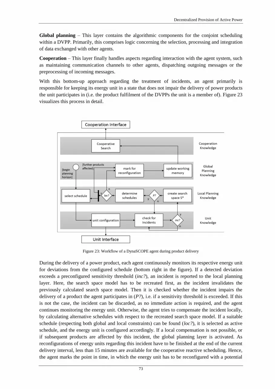
Decentralized Provision of Active Power
73
Global planning – This layer contains the algorithmic components for the conjoint scheduling
within a DVPP. Primarily, this comprises logic concerning the selection, processing and integration
of data exchanged with other agents.
Cooperation – This layer finally handles aspects regarding interaction with the agent system, such
as maintaining communication channels to other agents, dispatching outgoing messages or the
preprocessing of incoming messages.
With this bottom-up approach regarding the treatment of incidents, an agent primarily is
responsible for keeping its energy unit in a state that does not impair the delivery of power products
the unit participates in (i.e. the product fulfilment of the DVPPs the unit is a member of). Figure 23
visualizes this process in detail.
Figure 23: Workflow of a DynaSCOPE agent during product delivery
During the delivery of a power product, each agent continuously monitors its respective energy unit
for deviations from the configured schedule (bottom right in the figure). If a detected deviation
exceeds a preconfigured sensitivity threshold (inc?), an incident is reported to the local planning
layer. Here, the search space model has to be recreated first, as the incident invalidates the
previously calculated search space model. Then it is checked whether the incident impairs the
delivery of a product the agent participates in (P?), i.e. if a sensitivity threshold is exceeded. If this
is not the case, the incident can be discarded, as no immediate action is required, and the agent
continues monitoring the energy unit. Otherwise, the agent tries to compensate the incident locally,
by calculating alternative schedules with respect to the recreated search space model. If a suitable
schedule (respecting both global and local constraints) can be found (loc?), it is selected as active
schedule, and the energy unit is configured accordingly. If a local compensation is not possible, or
if subsequent products are affected by this incident, the global planning layer is activated. As
reconfigurations of energy units regarding this incident have to be finished at the end of the current
delivery interval, less than 15 minutes are available for the cooperative reactive scheduling. Hence,
the agent marks the point in time, in which the energy unit has to be reconfigured with a potential

Smart Nord Final Report
74
alternative schedule at the latest. Then the incident is inserted into the global planning knowledge,
which subsequently is sent to neighbouring agents, in order to begin the cooperative scheduling
process based on the COHDA heuristic.
Figure 24: Cooperative problem solving after the occurrence of incidents
In this experiment, a total number of 10 incidents (CHP outages for 30 minutes each) was
simulated. The arrows in the figure depict the detection of incidents. The incidents occurred
randomly during product delivery, thus some of them were detected simultaneously by the agents.
In Figure 25, the results from a series of experiments with different amounts of incidents in the
same DVPP as above is shown. Each experiment was repeated 100 times with different random
placements of the incidents.
Figure 25: Actual product fulfilment after the occurrence of incidents
Obviously, the final product quality deteriorates steadily with an increasing amount of incidents.
However, the analysis of the raw simulation data reveals that, in all shown cases, the triggered
rescheduling processes yield far superior product qualities in total than in the case without a
rescheduling.
Regarding the integration of costs, the following global objective function is set up:
𝑓(𝛾𝜓) = (1 − 𝛼) ⋅ 𝑞𝑒𝑝+ 𝛼 ⋅
1
𝑐𝜓 , 𝑐𝜓 > 0

Decentralized Provision of Active Power
75
Here, 𝛾𝜓 describes a solution candidate with respect to the DVPP denoted by 𝜓. The product
fulfilment criterion is identified by 𝑞𝑒𝑝, while 𝑐𝜓 depicts the associated costs. Then 𝛼 constitutes a
weighting factor, such that both optimization criteria are combined using a convex combination. In
Figure 26, the results from a series of experiments with different values for 𝛼 are visualized.
Figure 26: Product fulfilment compared to PV share with respect to the weighting coefficient
Each experiment in this series comprises 100 energy units, divided into 69 PV systems and 31 CHP
units. For the former, a cost factor of 0.0 ct/kWh was assumed, while for the latter 0.20 ct/kWh
was assumed. For each value of 𝛼, a total of 100 simulation runs have been performed. The results
show a substantial increase in the share of PV power in the final product delivery with increasing
significance of the costs. Meanwhile, the product fulfilment criterion deteriorates predominantly in
terms of outliers when preferring costs over product compliance.
Finally, in addition to the self-organized treatment of incidents with DynaSCOPE, a heuristic
method for estimating the effects of a scheduling action on the grid was developed. This allows
approaches like DynaSCOPE to account for required ancillary services due to rescheduling directly
in the objective function of the optimization algorithm. The method comprises a grid related cluster
schedule resemblance as a metric to analyse the grid usage changes using a graph based approach,
as depicted in Figure 27.

Smart Nord Final Report
76
Figure 27: Grid related cluster schedule resemblance. Left: Exemplary medium-voltage grid, showing an incident at
node 2. Right: A weighted graph representation of the grid upon the incident.
This metric can be used to compare different rescheduling options regarding grid usage for both
dynamic clusters of distributed energy resources and for rescheduling of static clusters like virtual
power plants. For more details, please refer to [77].
5 Conclusion and Outlook
The results of this work package clearly show the feasibility of implementing the continuous
scheduling for tracking and updating the operations of a DVPP to ensure product fulfilment at any
time during delivery in a fully distributed way. For the first time, a fully distributed method has
been developed which ensures feasible cluster schedules dynamically after incidents during product
delivery. All results from validation scenarios, which will be published soon as [78], show suitable
behaviour regarding performance and scalability.
However, improvements are still to be made considering the dependencies between different
consecutive DVPP if units are member in more than one cluster. In this case, controller conflicts
emerge during optimization due to interference for other clusters’ re-scheduling. Further studies are
needed to find an optimal balance between the frequency of dynamic reconfigurations of DVPPs
and efficient scheduling of units.
As a closing remark for this work package it should be noted, that this approach of distributed re-
scheduling of units could also be applied to schedule supply and demand in a micro grid
minimizing its residual load.

Decentralized Provision of Active Power
77
Work Package 1.5: Information Security in Agent-Based Energy
Management Systems
Christine Rosinger25
and Mathias Uslar25
1 Goals and Integration in the Sub-Project
Overall goal of this work package 1.5 (WP 1.5) is the improvement of security for agent-based
energy management systems. Therefore, this WP elaborated results in the following three main
topics of information security in the energy domain: security consideration in general, a data
privacy concept and a conceptualization of a trust model to support the coalition formation process
of the energy agents, which is the main part of this WP.
The reorganization from a monopolistic electricity market to a distributed smart grid and also the
liberalization of this market with its unbundling induces the need of more information and
communication technologies (ICT) [79]. The increasing ICT leads to a higher threat potential, as a
result of new and more intelligent actors and additional interfaces and data exchange that are
introduced in the energy domain [80]. Thus, the energy domain requires more revised and in some
cases even new security measures because of the special requirements of the energy domain [81].
Because of former non-existence of ICT for power supply, data privacy legislation was also not an
issue in this domain. With the upcoming Smart Grid, more individual-related data is exchanged in
this field. For example, in a continuous metering scenario with assumed quarter-hourly
measurement data transfers, there are 35,040 transmissions per household/meter per year [82].
Especially the prevention of profiling of households needs new privacy protection concepts.
The main motivation using a trust model is the occurrence of malicious agents. Different attack
motivations [83] like e.g. achieving economic advantages can mislead malicious agents to misuse
the system for their own advantage. In a so called worst case scenario, malicious agents can create
a system blackout if they cooperate as a so called botnet. To thwart such attacks, the application of
a reputation or a trust system [84] shall prevent this. Additionally, such a trust model should restrict
the actions of the malicious agents and acts as one security measure, respectively, increases
information security.
The three described topics of this WP act as cross-departmental function in this project because
security always addresses every layer in an ICT infrastructure. The developed trust model is used in
the coalition formation processes in work package 1.2 of sub-project one as one criterion for the
decision making of going into a coalition with one special agent or not. Overall, the developed
results in this WP 1.5 lead to a more robust and resilient system.
2 Related Work
Related work in the context of this work package focusses upon security, privacy and trust related
issues. In general, the following initiatives and projects could be identified and classified into the
categories of Smart Grid Security in general, data privacy, trust models and information security.
In the field of Smart Grid Security in general, the following references were mainly considered:
The “Protection Profile for the Gateway of a Smart Metering System” [85] by the Federal Office
for Information Security, Germany; the IEC 62351 with the title “Power systems management and
25
OFFIS – Institute for Information Technology, 26121 Oldenburg, Germany
[email protected], R&D Division Energy

Smart Nord Final Report
78
associated information exchange - Data and communications security” [86]; the ISO/IEC 27019
[87] as the domain specific component of the ISO 27k series with the title “Information security
management guidelines based on ISO/IEC 27002 for process control systems specific to the energy
utility industry”; and the NISTIR 7628 [88] with the title “Guidelines for Smart Grid Cyber
Security” which gives recommendations for security issues in the energy domain. Additionally
besides only security topics and standards, standardization of smart grids has to be considered [89].
Besides the previous mentioned literature, for the trustworthiness facet information security there
was some common security literature: For the assessment of security realizations, security metrics
were used [90]. To realize an improvement over existing systems or even in the development of
architectures, risk analyses [91], [92] and principles like security by design [79] were applied.
For data protection and privacy concerns for the smart grid domain also the NISTIR 7628 [88], and
several further publications [82], [85], [93], [94] were considered. Additionally, some sources for
metrics were necessary [90], [95].
Trust related literature can be divided into references for common trust considerations [96], [97],
[98], [99], trust in multi-agent systems [100], [101] and also the results and publication of the
DFG-funded project OC-TRUST [102], [103], [104] were in main focus in this work package.
3 Methodology
For this work package, the methodology and processes applied can be defined as follows. Even in
the methodology the three main topics security, privacy and trust can be identified, as can be seen
in the illustration of the methodology in Figure 28. The common security considerations were
derived from risk analysis standards and a classification was created. Of particular importance was
the application of a risk analysis for the yellow pages agent as a critical part of the Smart Nord
architecture. Additionally, an emphasis was on the privacy concept, creating a categorization with
eight levels to be applied in Smart Nord. This classification provides an analysis of the interfaces
exchanging critical data. Afterwards, the trust model is developed for the trustworthy coalition
formation of time-table-based active power provision taking into account the identified
trustworthiness facets. The next section will describe the most important aspects and results from
the three main pillars.
Figure 28: Methodology of WP 1.5

Decentralized Provision of Active Power
79
4 Main Results
As described before, the results of this work package 1.5 are divided into three parts: a common
security consideration, a privacy concept and a trust model for the coalizing energy agents. The
results of these topics are described in this section.
4.1 Common Security Considerations
Attackers have motivations and use security vulnerabilities to penetrate a system and to reach their
goal(s). They are endangering the compliance to different security goals. In the operational
scenario of the project are three different agent types – unit, market, and grid agents – which have
different goals as malicious agents. Another important factor for security is the attacker’s origin,
i.e. if he is an intrinsic or extrinsic attacker. In this work package several threat scenarios were
identified which cover different categories in various combinations, as can be seen in [83]. This
threat identification is derived by common risk analyses of security standards by BSI or NIST [89].
Beyond the threat identification, a common security analysis for the yellow pages agent – who
operates as directory service26 for the coalizing agents – mostly for the security goal authentication
was executed for different use cases of the yellow pages agent. This analysis identifies and treats
security issues of the yellow pages agent. A conclusion of this analysis is shown in Table 5.
Nr. Title Threat Security Measures
1
Registration
at yellow
pages agent
Entering malicious agent data reduces
benefit of yellow pages, can in worst
case lead to system breakdown.
First authentication via Postident procedure
or eID of ID card or passport; creation of
organizational or monetary obstacle
2 Status-
Response
Notification of wrong/not-its-own-
data results bad quality of service. Min. identification via login and password
3 Updating of
data
Update of not own data can lead to
wrong search results. Min. identification via login and password
4 Sign-Out
Sign-Out of another unit than the own
unit leads to gaps in the database of
the directory service.
Min. identification via login and password
5 Search
request
Using search requests not for coalition
formation but for data collection.
Restriction of frequency and only local
search results; cannot be avoided
completely
Table 5: Security consideration of the yellow pages agent
4.2 Data Privacy Concept for Energy Agents
The data privacy concept can be applied for the development of ICT architectures as privacy-by-
design principle. With this concept, exchanged data of energy agents in coalition formation
processes are analysed and categorized to identify the privacy risk of one particular date. With that
categorization further privacy measures can be recommended.
After a first draft of the ICT architecture, this concept can be applied for the analysis of the
exchanged data to categorize the degree of personalization. For this, a metric is used which is based
on security metrics of security compliance monitoring. The eight categories of the analysis – where
from category 1 to 8 the need of privacy measures increases – are:
26
Further realization of the yellow pages agent and the corresponding directory service can be seen in
WP2.3.

Smart Nord Final Report
80
Cat. 1: Date is not individual-related.
Cat. 2: Date is individual-related with several additional external sources.
Cat. 3: Date is individual-related with one additional external source.
Cat. 4: Date is individual-related with several additional intern sources.
Cat. 5: Date is individual-related with one additional intern source.
Cat. 6: Date is individual-related with several additional sources of the coalition formation process.
Cat. 7: Date is individual-related with one additional source of the coalition formation process.
Cat. 8: Date is individual-related without any additional sources.
The privacy metric analyses the quantity of privacy relevant data for one communication
relationship. The following Table 6 shows an example for the categorization of the exchanged data
of an agent for a photovoltaic plant in a coalition formation process. With that categorization the
privacy risk can be identified and used for privacy measures recommendations – like for example
reducing the exchanged data or encrypt the data – to get a privacy compliant communication.
Date
Categories
1 2 3 4 5 6 7 8
IP address X
Location X
Max. power X
Power forecast X
Total 2 0 1 0 1 0 0 0
Table 6: Data privacy categorization for energy agent
4.3 Trust Model for Coalizing Energy Agents
The trust model which was developed in this WP 1.5 supports the trustworthy coalition formation
of time-table-based active power provision and is the main part of this work package. The process
of the coalition formation, where this trust model is applied, is illustrated in work package 1.2 of
this sub-project one. The trust model consists of two parts: the structure and the application of the
trust model which will be described in the next paragraphs.
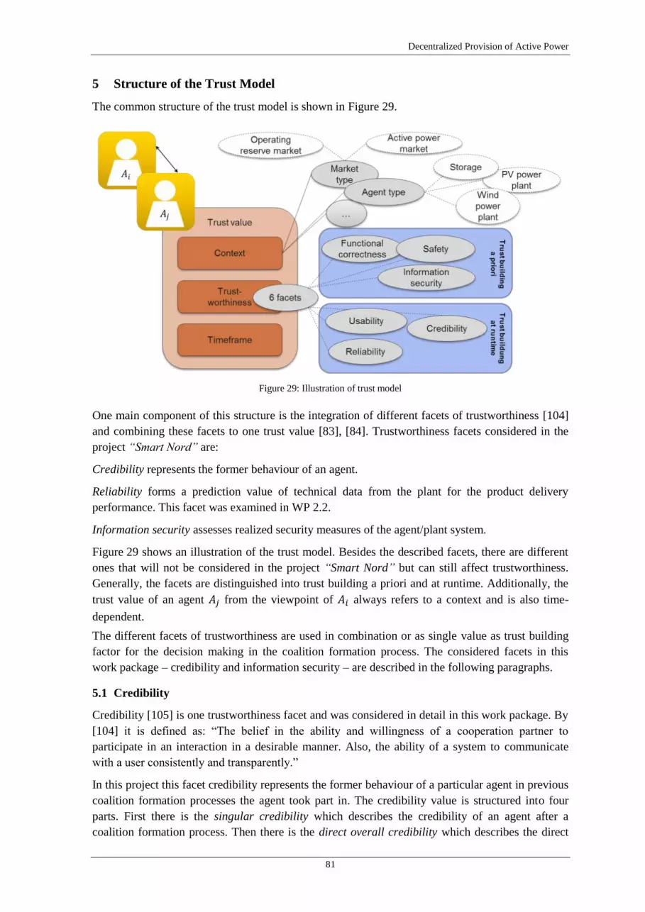
Decentralized Provision of Active Power
81
5 Structure of the Trust Model
The common structure of the trust model is shown in Figure 29.
Figure 29: Illustration of trust model
One main component of this structure is the integration of different facets of trustworthiness [104]
and combining these facets to one trust value [83], [84]. Trustworthiness facets considered in the
project “Smart Nord” are:
Credibility represents the former behaviour of an agent.
Reliability forms a prediction value of technical data from the plant for the product delivery
performance. This facet was examined in WP 2.2.
Information security assesses realized security measures of the agent/plant system.
Figure 29 shows an illustration of the trust model. Besides the described facets, there are different
ones that will not be considered in the project “Smart Nord” but can still affect trustworthiness.
Generally, the facets are distinguished into trust building a priori and at runtime. Additionally, the
trust value of an agent 𝐴𝑗 from the viewpoint of 𝐴𝑖 always refers to a context and is also time-
dependent.
The different facets of trustworthiness are used in combination or as single value as trust building
factor for the decision making in the coalition formation process. The considered facets in this
work package – credibility and information security – are described in the following paragraphs.
5.1 Credibility
Credibility [105] is one trustworthiness facet and was considered in detail in this work package. By
[104] it is defined as: “The belief in the ability and willingness of a cooperation partner to
participate in an interaction in a desirable manner. Also, the ability of a system to communicate
with a user consistently and transparently.”
In this project this facet credibility represents the former behaviour of a particular agent in previous
coalition formation processes the agent took part in. The credibility value is structured into four
parts. First there is the singular credibility which describes the credibility of an agent after a
coalition formation process. Then there is the direct overall credibility which describes the direct

Smart Nord Final Report
82
experiences (of singular credibility) in a relationship between one agent and another developed
over a time period. The third part is the indirect overall credibility which describes
recommendations of other agent to another agent over a time period. Finally, the overall credibility
comprises the direct and indirect relationships and calculated an overall credibility value for an
agent. In the following enumeration the different parts of the credibility value are described:
Singular Credibility: Singular credibility depends on the percentage contribution in a coalition
formation process – a higher percentage contribution means higher credibility – and the estimated
reliability – a higher estimated reliability means a lower credibility. For the singular credibility
between two agents the following formula is assumed: ))1((,1),( yxxMINyxfz .
As result, the value 0 means a minimal credibility and the value 1 means a maximum credibility.
Direct credibility: Direct credibility of one agent Ai to another agent Aj over a number of coalition
formations is built on own experiences. The formula for direct credibility is applied as follows:
)),((#
),(),(
ji
ji
ji
d ir
a llAAC
AACAAC
which means a mean value over all direct experiences agent Ai has
about Aj. Figure 30 shows the development of the value over a time period in four different use
cases.
Figure 30: Example of direct overall credibility
Indirect credibility: The indirect credibility is built on recommendations from other agents. This
value can be used if an agent has no direct experiences with another agent with whom the agent
wants to form a coalition with or if the agents wants to improve the own value. The formula for the
indirect overall credibility – where the agents Aj‘s recommendation of Ak is weighted by the direct
trust relationship between Ai and Aj – is applied as follows:
N
n
kn
dir
allni
dir
allki
ind
all AACAACN
AAC1
),(),(1
),(
Figure 31 shows how the agents are interrelated for the direct and indirect trust relationships.

Decentralized Provision of Active Power
83
Figure 31: Direct and indirect relationship
Overall credibility: The overall credibility combines the direct and indirect overall credibility. The
combined formula (1) is applied as follows:
xAACifAACAAC
AACifAAC
xAACifAAC
AAC
jiji
ind
allji
dir
all
jiji
ind
all
jiji
dir
all
jiall
),(0,),(),(2
1
0),(#),,(
),(#),,(
),(
(1)
This formula shows if an agent has a certain number x of direct experiences with agent Aj the agent
can use only the direct credibility, if the agent has no direct experiences he can use only the indirect
credibility and if he has some direct experiences but wants to improve this value by
recommendations the agent can use a combination of both – direct and indirect – credibility.
Figure 32 shows an example of the overall credibility of an agent with the use case aimed attack
from the view of another agent compared to the agent’s direct credibility. This shows that the usage
of recommendations by others can help getting a more precise value.
Figure 32: Example of overall credibility
5.2 Information Security
Information security [106] is one of the previous described trustworthiness facets which were
examined in particular in this WP. This facet takes into account that the more security measures a
system of an agent applies, the higher is the assumed trustworthiness of the agent. Additionally, for
this information security facet it is expected that if an agent realizes its security measures in a
standard-based way, the agent is considered more trustworthy. Information security as
trustworthiness facet can be used as trust building a priori or as a factor for the initial trust. In the
following two sections the concept of the security assessment is described.
Basic security assessment model
In Figure 33 an overview of the basic security assessment model as ontology is depicted.

Smart Nord Final Report
84
(B)
(A)
(C)
(D)
Security measure
Security attack
threatens
Eavesdropping
Denial
Tampering
Masquerade
Replay
Security requirement
Non-repudiation
IntegrityConfidentiality
Authenticity
Availability
threatens threatens threatens threatens
Access Control
Network Security
prevents
Security Standards
IEC 62351ISO 27000 BSI 100
IEC 62351-4 IEC 62351-3IEC 62351-7
supports
IEC 62351-6IEC 62351-5
Cyptography
supports
Threat scenario
consistsOf
Attacker typeexecutes
Securiy Assessment
modelassesses
concerns
CommonDomain specific
Energynationalinternational
Security value
calculates
prevents
Security technology
Organizational Security & Risk Management
Security Architecture
IEC 62351-10
supports
supports
ISO 27019
NERC CIP
prevents
supports
Legend Superclass
Subclasses
Generalization
Correlation
Date/Value
Figure 33: Assessment of implemented information security measures
The solid lines represent hierarchical relationships between the concepts shown in blue and red-
striped boxes and the dashed lines are object-property relationships, which can be reasoned. The
green oval shows the security value which is calculated by the security assessment model and
which represents the result of the assessment phase.
The basic security assessment model in Figure 33 is segmented into four parts. Part (A) shows
different security attacks while part (B) shows several security requirements. Part (C) shows
security measures which are related with the appropriate security standards depicted in part (D).
Even in part (C) – the most relevant concept for this assessment – the security assessment model
concept is associated with the security measure concept over the object property assesses. Finally,
this security assessment model concept with its assessment functions realizes the overall security
value. A more detailed description of this model can be found in [106].
Security value assessment method
Security assessment consists of assumptions because there are always different requirements and
every user has to decide by oneself which security requirements are the most important for his
particular use case. The security assessment method is based on a regular risk analysis [91], [92]
with the assumption that the more security requirements are covered the more trustworthiness can
be expected. Thus, the security assessment per agent consists of three parts: The assessment per
security requirement 𝐴, the consideration of security standards 𝑆𝑡 and a weighting factor 𝑃𝑟𝑖𝑜. For
the final security assessment per agent 𝑆𝑒𝑐(𝐴𝑔𝑒𝑛𝑡) a weighted average with the single assessment
per security requirement 𝐴(𝑖), the assessment of standard-based realization per security
requirement 𝑆𝑡(𝑖), and the priority per security requirement 𝑃𝑟𝑖𝑜(𝑖) can be built which can be seen
in formula (2). #𝑠𝑒𝑐𝑟𝑒𝑞 implies in this case the number of security requirements.

Decentralized Provision of Active Power
85
𝑆𝑒𝑐(𝐴𝑔𝑒𝑛𝑡) =∑ 𝐴(𝑖)∗𝑆𝑡(𝑖)∗𝑃𝑟𝑖𝑜(𝑖)#𝑠𝑒𝑐𝑟𝑒𝑞
𝑖=1
∑ 𝑃𝑟𝑖𝑜(𝑗)#𝑠𝑒𝑐𝑟𝑒𝑞𝑗=1
(2)
6 Application of the Trust Model
The second main part of the trust model is the consideration of different phases a trust value has to
go through during its lifecycle, which is shown in Figure 34.
Figure 34: Life cycle of the trust model
The first appearance of a trust value is in the initial trust phase. This occurs when an agent is
generated or joins the community. In this phase it has to be decided and determined which value
the trustworthiness will be. Facets that have a trust building a priori can be applied in this initial
trust phase. After this, the calculation or update phase takes place where e.g. the former behaviour
of an agent is regarded. This behaviour is then included into the value or the value is updated. The
storage phase considers where and how the different facets are stored and how tampering can be
prevented. After a value was stored, there is a relationship back to the calculation and update phase
because this is the main life circle of the value. After storage there are different other possibilities
what happens next with the value. The exchange/distribution phase is concerned with the method
how the values are exchanged and distributed between the agents and also a secure transfer of the
values is considered. In the utilization phase, the different facets of the trust value are combined,
goal functions are applied and guidance recommendations are given. If a value is compromised by
malicious agents, revocation of the value has to be initiated.
7 Conclusion and Outlook
This work package examined different issues from the security domain for energy related topics
especially for coalition formation processes of energy agents in a multi-agent system. Several
results were elaborated like a trust model and common security and privacy analyses for coalition
formation processes of energy agents. We showed some approaches for security considerations,
like the appropriate threat scenarios and the security consideration of the yellow pages agent. The
privacy concept supports the privacy-by-design-principle and shows a categorization of individual-
related data in this use case. Finally, the trust model represents the main part of this work package
which is divided into the structure and the application of the trust model. In this trust model the
trustworthiness facets credibility and information security were examined primarily. The concepts
of these facets were also described in the “main results” section of this chapter.
For further work, the security and privacy concepts has to be examined empirically. Additionally
for the trust model, a combination of different trustworthiness facets has to be considered, for
example how different facets should be weighted or in which phase of the life cycle of the trust
model diverse facets can be utilized. Additionally, an integration of this model into the existing

Smart Nord Final Report
86
NIST measures, described in e.g. [107] has to be evaluated. Secure storage and avoiding of
manipulated exchange of the several trust values has also be considered in the future.
References
[1] A. Nieße, S. Beer, J. Bremer, C. Hinrichs, O. Lünsdorf, M. Sonnenschein, “Conjoint Dynamic
Aggregation and Scheduling Methods for Dynamic Virtual Power Plants,” In Proceedings of the 2014
Federated Conference on Computer Science and Information Systems, pp. 1505-1514.
[2] O. Abarrategui, J. Marti, A. Gonzalez, “Constructing the Active European Power Grid,” in
Proceedings of WCPEE09, Cairo, 2009, pp. 1–4.
[3] A. Nieße, S. Lehnhoff, M. Tröschel, M. Uslar, C. Wissing, H.-J. Appelrath, M. Sonnenschein,
“Market-based self-organized provision of active power and ancillary services: An agent-based
approach for smart distribution grids,” in Complexity in Engineering (COMPENG), 2012.
[4] Bundesnetzagentur, “’Smart Grid’ and ’Smart Market’,” 2012.
[5] F. Wu, K. Moslehi, A. Bose, “Power system control centers: Past, present, and future,” Proceedings of
the IEEE, vol. 93, no. 11, pp. 1890–1908, 2005.
[6] International Energy Agency, “Distributed Generation in Liberalised Electricity Markets,” OECD
Publishing, 2002.
[7] S. Awerbuch, A. M. Preston, Eds., “The Virtual Utility: Accounting, Technology & Competitive
Aspects of the Emerging Industry,” ser. Topics in Regulatory Economics and Policy. Kluwer
Academic Publishers, 1997, vol. 26.
[8] D. Coll-Mayor, R. Picos, E. Garciá-Moreno, “State of the art of the virtual utility: the smart
distributed generation network,” International Journal of Energy Research, vol. 28, no. 1, pp. 65–80,
2004.
[9] S. McArthur, E. Davidson, V. Catterson, A. Dimeas, N. Hatziargyriou, F. Ponci, T. Funabashi,
“Multi-agent systems for power engineering applications – Part I: Concepts, approaches, and technical
challenges,” IEEE Transactions on Power Systems, vol. 22, no. 4, pp. 1743–1752, 2007.
[10] R. R. Negenborn, Z. Lukszo, H. Hellendoorn, Eds., “Intelligent Infrastructures,” ser. Intelligent
Systems, Control and Automation: Science and Engineering. Springer, 2010, vol. 42.
[11] S. D. Ramchurn, P. Vytelingum, A. Rogers, N. R. Jennings, “Agentbased homeostatic control for
green energy in the smart grid,” ACM Trans. Intell. Syst. Technol., vol. 2, no. 4, pp. 35:1–35:28, Jul.
2011.
[12] G. Anders, F. Siefert, J.-P. Steghöfer, H. Seebach, F. Nafz, W. Reif, “Structuring and Controlling
Distributed Power Sources by Autonomous Virtual Power Plants,” in IEEE Power and Energy Student
Summit (PESS 2010). IEEE Power & Energy Society, 2010.
[13] “Putting the ’smarts’ into the smart grid: A grand challenge for artificial intelligence,” Commun.
ACM, vol. 55, no. 4, pp. 86–97, Apr. 2012.
[14] A. Nieße, M. Tröschel, M. Sonnenschein, “Designing Dependable and Sustainable Smart Grids - How
to Apply Algorithm Engineering to Distributed Control in Power Systems,” Environmental Modelling
and Software, vol. 56, pp. 37-51, 2014.
[15] A. Nieße, S. Lehnhoff, M. Sonnenschein, M. Tröschel, “Dynamic Virtual Power Plants in Future
Energy Grids: Defining the Gap to the Field,” in Proceedings VDE Kongress 2014, VDE Verlag.
[16] H.-J. Appelrath, H. Kagermann, C. Mayer Eds., “Future Energy Grid (acatech study),” acatech,
Munich, 2012.
[17] F. Korb, S. Lehnhoff, C. Mayer, M. Uslar, “Data Access-Point Manager – definierte
Informationsflüsse für Betriebsführung und Markt,” Energiewirtschaftliche Tagesfragen, 64(3), 2014.
[18] The Smart Grid Interoperability Panel Cyber Security Working Group. Introduction to NISTIR 7628
Guidelines for Smart Grid Cyber Security, 2010.
[19] U. Richter, M. Mnif, J. Branke, C. Müller-Schloer, H. Schmeck, “Towards a Generic
Observer/Controller Architecture for Organic Computing,” in Informatik 2006. LNI P-93, pp. 112-
119, 2006.
[20] J. Psola et al., “Modeling of a Redox Flow Battery Storage for Grid Applications,” in PCIMasia 2013,
Shanghai, China, 2013.
[21] J. Psola et al., “Optimization of energy output by combining energy storages with renewable
energies,” in PCIMasia 2014, Shanghai, China, 2014.

Decentralized Provision of Active Power
87
[22] J. Widén, “Correlation Between Large-Scale Solar and Wind Power in a Future Scenario for Sweden,”
in. IEEE Transactions on Sustainable Energy, Vol. 2, No. 2, p. 177-184, 2011.
[23] J. Psola et al., “Technologies and Operational Concepts for Energy Storages,” in EnviroInfo 2013,
Hamburg, Germany, 2013.
[24] J. Psola, W. Canders, “Klassifizierung von Energiespeichern,” in FEN - Bericht des IMAB zum TP2,
Braunschweig, Germany, 2009.
[25] H. L. Ferreira et al., “Characterisation of electrical energy storage technologies,” in Energy 53 (2013),
p. 288-298, 2013.
[26] F. Díaz-González et al., “A review of energy storage technologies for wind power applications,” in:
Renewable and Sustainable Energy Reviews 16 (2012), p. 2154-2171, 2012.
[27] H. Chen et al., “Progress in electrical energy storage systems: A critical review,” in Progress in
Natural Science 19 (2009), p. 291-312, 2009.
[28] Y. Shoham, K. Leyton-Brown, “Multiagent Systems: Algorithmic, Game-Theoretic, and Logical
Foundations,” Cambridge University Press, 2000.
[29] T. Sandholm, K. Larson, M. Andersson, O. Shehory, F. Thomé, “Coalition structure generation with
worst case guarantees,” in Artificial Intelligence, 111, 209-238.
[30] T. Rahwan, N. R. Jennings, “An Improved Dynamic Programming Algorithm for Coalition Structure
Generation,” in Proc. of 7th Int. Conf. on Autonomous Agents and Multiagent Systems, 2008.
[31] M. H. Rothkopf, A. Pekei, R. M. Harstad, “Computationally Manageable Combinatorial Auctions,”
Center for Discrete Mathematics & Theoretical Computer Science, 1995.
[32] V. D. Dang, N. R. Jennings, “Generating coalition structures with finite bound from the optimal
guarantees,” in 3rd International Conference on Autonomous Agents and Multi-Agent Systems, 2004.
[33] T. Rahwan, S. Ramchurn, N. Jennings, A. Giovannucci, “An Anytime Algorithm for Optimal
Coalition Structure Generation,” in Journal of Artificial Intelligence Research (JAIR), 34, 521–567,
2009.
[34] T. Michalak, J. Sroka, T. Rahwan, J. Wooldridge, P. McBurney, N. R. Jennings, “A Distributed
Algorithm for Anytime Coalition Structure Generation,” in Proc. of 9th Int. Conf. on Autonomous
Agents and Multiagent Systems (AAMAS 2010), 2010.
[35] O. Shehory, S. Kraus, “Methods for task allocation via agent coalition formation,” in Artificial
Intelligence, 101, 165-200, 1998.
[36] S. Sen, P. S. Dutta, “Searching for optimal coalition structures,” in Proceedings of the Fourth
International Conference on MultiAgent Systems, 2000.
[37] C. Rosinger, S. Beer, “Glaubwürdigkeit in dynamischen Wirkleistungsverbünden,” in Informatik-
Spektrum, 2014, pp. 1-8.
[38] R. G. Smith, “The Contract Net Protocol: High-Level Communication and Control in a Distributed
Problem Solver,” in IEEE Transactions on Computers, C-29(12), 1104–1113.
[39] S. S. Fatima, M. Wooldridge, N. R. Jennings, “A Linear Approximation Method for the Shapley
Value,” in Artificial Intelligence, 172, 1673-1699.
[40] S. Beer, “Dynamic Coalition Formation in Electricity Markets,” PHD thesis, Dept. of Computing
Science, University of Oldenburg, Oldenburg, Niedersachsen, planned to be submitted 2015-04.
[41] S. Beer, “A Formal Model for Agent-based Coalition Formation in Electricity Markets,” in 4th
IEEE/PES Innovative Smart Grid Technologies Europe (ISGT EUROPE), Kopenhagen, pp. 1-5,
2013.
[42] A. Nieße, S. Lehnhoff, M. Tröschel, M. Uslar, C. Wissing, H.-J. Appelrath, M. Sonnenschein,
“Market–Based Self–Organized Provision of Active Power and Ancillary Services,” IEEE, 06 2012.
[43] M. Blank, S. Gerwinn, O. Krause, S. Lehnhoff, “Support Vector Machines for an efficient
Representation of Voltage Band Constraints,” in Innovative Smart Grid Technologies. IEEE PES,
2011.
[44] J. Bremer, B. Rapp, M. Sonnenschein, “Support Vector based Encoding of Distributed Energy
Resources’ Feasible Load Spaces,” in IEEE PES Conference on Innovative Smart Grid Technologies
Europe, Chalmers Lindholmen, Gothenburg,Sweden, 2010.
[45] Z. Michalewicz, M. Schoenauer, “Evolutionary algorithms for constrained parameter optimization
problems,” Evol. Comput., 4:1–32, March 1996.
[46] G. E. Liepins, M. D. Vose, “Representational issues in genetic optimization,” in Journal of
Experimental and Theoretical Artificial Intelligence, 2, 1990.

Smart Nord Final Report
88
[47] C. A. Coello Coello, “Theoretical and numerical constraint-handling techniques used with
evolutionary algorithms: a survey of the state of the art,” Computer Methods in Applied Mechanics
and Engineering, 191(11-12):1245–1287, January 2002.
[48] O. Kramer, “A review of constraint-handling techniques for evolution strategies,” Appl. Comp. Intell.
Soft Comput., 2010:1–19, January 2010.
[49] S. Koziel, Z. Michalewicz, “Evolutionary algorithms, homomorphous mappings, and constrained
parameter optimization,” Evol. Comput., 7:19–44,March 1999.
[50] D. G. Kim, “Riemann mapping based constraint handling for evolutionary search,” in SAC, pages
379–385, 1998.
[51] W. Squire, “Computer implementation of the schwarz-christoffel transformation,” Journal of the
Franklin Institute, 299(5):315322, 1975.
[52] J. W. Bandler, R. M. Biernacki, S. H. Chen, P. A. Grobelny, R. H. Hemmers, “Space mapping
technique for electromagnetic optimization,” Microwave Theory and Techniques, IEEE Transactions
on, 42(12):2536–2544, 1994.
[53] J. W. Bandler, R. M. Biernacki, S. H. Chen, R. H. Hemmers, K. Madsen, “Electromagnetic
optimization exploiting aggressive space mapping,” Microwave Theory and Techniques, IEEE
Transactions on, 43(12):2874–2882, 1995.
[54] J. Bremer, M. Sonnenschein, “A Distributed Greedy Algorithm for Constraint-based Scheduling of
Energy Resources,” in Maria Ganzha, Leszek A. Maciaszek,and Marcin Paprzycki, editors, Federated
Conference on Computer Science and Information Systems - FedCSIS 2012, Wroclaw, Poland, 9-12
September 2012,Proceedings, pages 1285–1292, 2012.
[55] J. Bremer, M. Sonnenschein, “Constraint-handling for Optimization with Support Vector Surrogate
Models – A Novel Decoder Approach,” in J. Filipe and A.L.N. Fred, editors, ICAART 2013 –
Proceedings of the 5th International Conference on Agents and Artificial Intelligence, volume 2,
pages 91–105, Barcelona, Spain, 2013.SciTePress.
[56] A. Hevner, S. March, J. Park, S. Ram, “Design Science in Information Systems Research,” MIS
Quarterly (28:1) 2004, pp. 75-105.
[57] J. Bremer, M. Sonnenschein, “Automatic Reconstruction of Performance Indicators from Support
Vector based Search Space Models in Distributed Real Power Planning Scenarios,” in M. Horbach
(Hrsg.): Lecture Notes in Informatics 220, Proceedings of the Informatik 2013 - Informatik angepasst
an Mensch, Organisation und Umwelt. 16.-20. September, Koblenz, Germany. LNI 220, ISBN 978-3-
88579-614-5, pp. 1441-1454, 2013.
[58] J. Bremer, M. Sonnenschein, “Model-based Integration of Constrained Search Spaces into Distributed
Planning of Active Power Provision,” Computer Science and Information Systems, Vol. 10, No. 4,
1823-1854, 2013.
[59] J. Bremer, M. Sonnenschein, “Sampling the Search Space of Energy Resources for Self-organized,
Agent-based Planning of Active Power Provision,” in B. Page, A.G. Fleischer, J. Göbel, V.
Wohlgemuth (Eds.): Environmental Informatics and Renewable Energies - 27th International
Conference on Informatics for Environmental Protection. Shaker Verlag, ISBN: 978-3-8440-1676-5,
pp. 214-222, 2013.
[60] A. Nieße, M. Tröschel, M. Sonnenschein, “Designing dependable and sustainable Smart Grids – How
to apply Algorithm Engineering to distributed control in power systems,” in Environmental Modelling
& Software, 2013
[61] D. M. J. Tax, R. P. W. Duin, “Data Domain Description using Support Vectors,” in European
Symposium on Artificial Neural Networks – ESANN, S. 251–256, 1999.
[62] A. Ben-Hur, H. T. Siegelmann, D. Horn, V. Vapnik, “Support Vector Clustering,” in Journal of
Machine Learning Research 2, S. 125–137, 2001.
[63] J. Bremer, B. Rapp, M. Sonnenschein, “Encoding distributed Search Spaces for Virtual Power
Plants,” in IEEE Symposium Series on Computational Intelligence 2011 (SSCI 2011). Paris, France,
April 2011.
[64] I. Steinwart, A. Christmann, “Support Vector Machines,” 1st. Springer Publishing Company,
Incorporated. ISBN: 0387772413, 2008.
[65] J. Bremer, M. Sonnenschein, “Parallel tempering for constrained many criteria optimization in
dynamic virtual power plants,” IEEE Symposium on Computational Intelligence Applications in
Smart Grid (CIASG). Doi: 10.1109/CIASG.2014.7011551, 2014

Decentralized Provision of Active Power
89
[66] C. Hinrichs, J. Bremer, M. Sonnenschein, “Distributed Hybrid Constraint Handling in Large Scale
Virtual Power Plants,” in IEEE PES Conference on Innovative Smart Grid Technologies Europe
(ISGT Europe 2013). IEEE Power & Energy Society, 2013.
[67] A. Nieße, S. Lehnhoff, M. Tröschel, M. Uslar, C. Wissing, H.-J. Appelrath, M. Sonnenschein,
“Market-based self-organized provision of active power and ancillary services: An agent-based
approach for Smart Distribution Grids,” in Complexity in Engineering (COMPENG), Aachen, 2012.
[68] G. Anders, F. Siefert, J.-P. Steghöfer, H. Seebach, F. Nafz, W. Reif, “Structuring and Controlling
Distributed Power Sources by Structuring and Controlling Distributed Power Sources by Autonomous
Virtual Power Plants,” in Proceedings of the IEEE Power and Energy Student Summit 2010.
[69] R. Li, J. Li, G. Poulton, “Agent-Based Optimisation Systems for Electrical Load Management,” in
The 20th Australian Joint Conference on Artificial Intelligence. Queensland, Australia.
[70] E. Pournaras, “Multi-level Reconfigurable Self-organization in Overlay Services,” Thesis,TU Delft.
2013.
[71] M. Tröschel, “Aktive Einsatzplanung in holonischen Virtuellen Kraftwerken,” Dissertation.
Universität Oldenburg. 2010.
[72] C. Hinrichs, S. Lehnhoff, M. Sonnenschein, “COHDA: A Combinatorial Optimization Heuristic for
Distributed Agents,” in Agents and Artificial Intelligence, Communications in Computer and
Information Science, vol. 449, J. Filipe and A. Fred, Eds. Berlin, Heidelberg: Springer Berlin
Heidelberg, 2014, pp. 23–29.
[73] E. Handschin, C. Rehtanz, H. F. Wedde, O. Krause, S. Lehnhoff, “On-line stable state determination
in decentralized power grid management,” in Proceedings of the 16th Power Systems Computation
Conference (PSCC’08), pages 07–14, Glasgow, Scotland, UK, 2008.
[74] O. Krause, S. Lehnhoff, “Generalized Static-State Estimation,” in 22nd Australasian Universities
Power Engineering Conference (AUPEC), 2012.
[75] J. Bremer, M. Sonnenschein, “Automatic Reconstruction of Performance Indicators from Support
Vector based Search Space Models in Distributed Real Power Planning Scenarios,” in Lecture Notes
in Informatics 220, Proceedings of the Informatik 2013 - Informatik angepasst an Mensch,
Organisation und Umwelt. Koblenz, Germany. pp. 1441-1454. 2013.
[76] M. Wooldridge, “Intelligent Agents,” in Multi-Agent Systems, 2nd ed., G. Weiss, Ed. MIT Press,
2013.
[77] A. Nieße, M. Sonnenschein, “Using Grid Related Cluster Schedule Resemblance for Energy
Rescheduling – Goals and Concepts for Rescheduling of Clusters in Decentralized Energy Systems,”
in SMARTGREENS, 2013.
[78] A. Nieße, “Verteilte kontinuierliche Einsatzplanung in Dynamischen Virtuellen Kraftwerken,” Ph.D.
thesis, Dept. of Computing Science, Univ. of Oldenburg, Germany (to appear 2015).
[79] M. Sonnenschein, H.-J. Appelrath, L. Hofmann, M. Kurrat, S. Lehnhoff, C. Mayer, A. Mertens,
M. Uslar, A. Nieße, M. Tröschel, “Dezentrale und selbstorganisierte Koordination in Smart Grids,”
VDE Kongress 2012.
[80] M. Postina, S. Rohjans, U. Steffens, M. Uslar, “Views on service oriented architectures in the context
of Smart Grids,” First IEEE international conference on Smart grid communications
(SmartGridComm), 2010.
[81] A. Suhr, C. Rosinger, H. Honecker, “System Design and Architecture – Essential Functional
Requirements vs. ICT Security in the energy domain,” Int. ETG-Kongress 2013 (ETG-FB 139), p. 9,
2013.
[82] A. Roßnagel, S. Jandt, “Datenschutzkonformes Energieinformationsnetz - Risiken und
Gestaltungsvorschläge,” DuD - Datenschutz und Datensicherheit, S. 373-378, 2010.
[83] C. Rosinger, M. Uslar, J. Sauer, “Threat Scenarios to evaluate Trustworthiness of Multi-agents in the
Energy Data Management,” EnviroInfo2013 – Environmental Informatics Renewable Energies, 2013.
[84] C. Rosinger, M. Uslar, F. Hockmann, “Reputationssysteme für selbstorganisierte Multi-Agenten-
Systeme in Energiemanagementsystemen,” VDE-Kongress 2012, 2012.
[85] Federal Office for Information Security, Germany, “BSI–CC–PP–0073: Protection Profile for the
Gateway of a Smart Metering System (Smart Meter Gateway PP)”, 2014.
[86] International Electrotechnical Commission (IEC), “IEC 62351 part 1 - 11, Power systems
management and associated information exchange - Data and communications security”, 2007 – 2013.

Smart Nord Final Report
90
[87] International Organization for Standardization (ISO), International Electrotechnical Commission
(IEC), “ISO/IEC TR 27019: Information technology - Security techniques - Information security
management guidelines based on ISO/IEC 27002 for process control systems specific to the energy
utility industry”, 2013.
[88] The Smart Grid Interoperability Panel Cyber Security Working Group, “NISTIR 7628 - Guidelines
for Smart Grid Cyber Security vol. 1-3,” August 2010.
[89] M. Uslar, M. Specht, C. Dänekas, J. Trefke, S. Rohjans, J. M. Gonzalez, C. Rosinger, R. Bleiker,
“Standardization in Smart Grids,” Springer Publishing, 2013.
[90] A. Jaquith, “Security Metrics: Replacing Fear, Uncertainty, and Doubt,” Addison-Wesley, 2007.
[91] International Organization for Standardization (ISO), “ISO 27005: Information technology —
Security techniques — Information security risk management”.
[92] CEN-CENELEC-ETSI Smart Grid Coordination Group, final document in mandate M/490 group
SGIS “Smart Grid Information Security”, 2012.
[93] D. Laupichler, S. Vollmer, H. Bast, M. Intemann, “Das BSI-Schutzprofil: Anforderungen an den
Datenschutz und die Datensicherheit für Smart Metering Systeme,” in DuD – Datenschutz und
Datensicherheit, 8:542 – 546, 2011.
[94] O. Raabe, M. Lorenz, F. Pallas, E. Weis, A. Malina, “14 Thesen zum Datenschutz im Smart Grid,” in
DuD – Datenschutz und Datensicherheit, 8:519 – 523, 2011.
[95] A. Sowa, “Metriken - der Schlüssel zum erfolgreichen Security und Compliance Monitoring,”
Wiesbaden: Vieweg + Teubner Verlag, 2011, ISBN 978–3–8348–1480–7.
[96] L. Capra, “Engineering human trust in mobile system collaborations,” in Proceedings of the 12th
ACM SIGSOFT twelfth international symposium on Foundations of software engineering, ACM
SIGSOFT Softw. Eng. Notes, p. 10, 2004.
[97] C. Castelfranchi, R. Falcone, “Trust theory: A socio-cognitive and computational model,” Wiley,
2010.
[98] A. Jøsang, “The right type of trust for distributed systems,” Proceeding NSPW ’96 Proc. 1996 Work.
New Secur. Paradigm., pp. 119–131, 1996.
[99] S. P Marsh, “Formalising trust as a computational concept,” PhD-Thesis University of Stirling, 1994.
[100] A. Das, M. M. Islam, “SecuredTrust: A Dynamic Trust Computation Model for Secured
Communication in Multiagent Systems,” IEEE Trans. Dependable Secur. Comput., vol. 9, no. 2, pp.
261–274, Mar. 2012.
[101] H. Yu, Z. Shen, C. Leung, C. Miao, V. R. Lesser, “A Survey of Multi-Agent Trust Management
Systems,” IEEE Access, vol. 1, pp. 35–50, 2013.
[102] R. Kiefhaber, S. Hammer, B. Savs, J. Schmitt, M. Roth, F. Kluge, E. Andre, T. Ungerer, “The
Neighbor-Trust Metric to Measure Reputation in Organic Computing Systems,” 2011 Fifth IEEE
Conf. Self-Adaptive Self-Organizing Syst. Work., pp. 41–46, Oct. 2011.
[103] R. Kiefhaber, G. Anders, F. Siefert, T. Ungerer, W. Reif, “Confidence as a Means to Assess the
Accuracy of Trust Values,” 2012 IEEE 11th Int. Conf. Trust. Secur. Priv. Comput. Commun., pp.
690–697, Jun. 2012.
[104] J.-P. Steghöfer, R. Kiefhaber, “Trustworthy organic computing systems: Challenges and
perspectives,” in Autonomic and Trusted Computing and Trusted Computing, Springer Berlin
Heidelberg, 2010.
[105] C. Rosinger, S. Beer, “Glaubwürdigkeit in dynamischen Wirkleistungsverbünden,” in Informatik-
Spektrum, pp. 1–8, Dezember 2014.
[106] C. Rosinger, M. Uslar, J. Sauer, “Using Information Security as a Facet of Trustworthiness for Self-
Organizing Agents in Energy Coalition Formation Processes,” EnviroInfo2014 – Environmental
Informatics Renewable Energies, 2014.
[107] M. Uslar, C. Rosinger, S. Schlegel, “Security by Design for the Smart Grid: Combining the SGAM
and NISTIR 7628,” IEEE 38th International Computer Software and Applications Conference
Workshops (COMPSACW), IEEE Publishing 2014.


Grid Stabilizing Ancillary Services
93
Sub-Project Two:
Grid Stabilizing Ancillary Services


Grid Stabilizing Ancillary Services
95
Overview on Sub-Project Two:
Grid Stabilizing Ancillary Services
Sebastian Lehnhoff27
, Marita Blank28
, Robert Bleiker27
, Thole Klingenberg27
, Klaus Piech27
,
Mathias Uslar27
, Walter Schumacher29
, Mauro Calabria29
, Axel Mertens30
, René Dietz30
and Felix Fuchs30
1 Goals
The increase in renewable power generation causes an overall decrease in conventional power
generation from large-scale and highly predictable fossil power plants. Aside from market-based
provision of active power schedules, these power plants are crucial for the provision of short-term
reactive ancillary services such as frequency and voltage control. Substituting these plants for
renewable generation units requires the latter to be capable of providing these ancillary services in
order to guarantee a reliable and stable power supply. In this sub-project key challenges of
providing reliable ancillary services from unreliable distributed renewable energy sources are
addressed:
Setting up coordinated coalitions for real-time provision of ancillary services
(work package 2.1)
Reliable contribution planning and risk management of coordinated coalitions for the provision
of ancillary services (work package 2.2)
Interoperability and performance issues of coalition formation for ancillary services
(work package 2.3)
Stability of automated controllers in ancillary service coalitions in low-voltage grids
(work package 2.4)
Grid-supporting services through inverters and stable lower-level control
(work package 2.5)
2 Related Work
Transforming the electric power system to incorporate an increasing share of renewable, distributed
generation implicates new challenges for the control of the system: control methods have to cope
with many individually configured, distributed, small generation units (photovoltaic (PV) systems,
combined heat and power plants (CHP), wind energy converters, etc.) as well as with the
fluctuation in their feed-in depending on foremost meteorological conditions. A paradigm shift
from the current centralized control method assuming a static set of large controllable power plants
to a decentralized, self-organized system of agents representing small active units (generators,
loads, storages) in the power supply system has been proposed by the Smart Grid community for
several years, and several self-organization approaches for coordinating these units have been
proposed [1], [2], [3], [4].
27
OFFIS – Institute for Information Technology 28
University of Oldenburg 29
Technische Universität Braunschweig 30
Leibniz Universität Hannover

Smart Nord Final Report
96
Compared with these approaches, within the Smart Nord project a method for agent-based
aggregation of distributed generation as well as consumer appliances into so called coordinated
coalitions has been developed that is not only capable of matching appropriate products at
traditional markets for active power schedules (e.g. day-ahead or intra-day) but additionally
capable of providing ancillary services to stabilize the grid. Additional related work relevant to
each work package is presented in the context of the appropriate following work packages.
3 Main Results
In order to enable coordinated coalitions to deliver ancillary services in real-time a hybrid approach
has been developed. At first each unit’s power contribution is estimated based on long-term as well
as (more reliable) short-term forecasts and coordinated coalitions are formed following economical
aspects. This communication-based (multi-agent system) economical optimization yields a
coordinated coalition – strictly adhering to a certain minimum reliability level – that is capable of
activating power reserves for stabilizing grid frequency (primary control reserve). In order to
guarantee short-term activation in real-time each unit parameterizes a local controller (droop)
through appropriate configuration of the connected inverter, which exhibits the desired behaviour
of a frequency-proportional power response. The main results of this sub-project are the
coordination formation algorithms, taking into account the reliability constraints of ancillary
services as well as inverter-based distributed controller design optimizing small-signal stability of
such coalitions [5], [6], [7], [8].
4 Conclusion and Outlook
While the sub-project has demonstrated that reliable and stable provision of primary control reserve
through appropriate inverter configuration is possible and can be operated following economical
targets of ancillary service markets, damping issues and small-signal stability has proven to be a
much more important challenge than initially expected. A PDT-controller has been designed to
optimize the dynamic behaviour of coordinated coalitions in low-voltage grids. However, it has
been proven that dynamic interactions between nodes of a power grid can turn the system unstable
and thus it is foreseeable that additional distributed controller optimization and damping
mechanisms are required when extending the frequency response regime with other controllers, e.g.
voltage/var control or schemes for optimal generation curtailment. These will not only introduce
more complex dynamics but very likely will influence each other, which has to be investigated
further.
Grid Stabilizing Ancillary Services
97
Work Package 2.1: Coordinated Coalitions for Real-time
Provision of Ancillary Services
Thole Klingenberg31
and Sebastian Lehnhoff31
1 Goals and Integration in the Sub-Project
Within this sub-project a method for agent-based aggregation of distributed generation as well as
consumer appliances into so called coordinated coalitions has been developed that is not only
capable of matching appropriate products at traditional markets for active power schedules (e.g.
day-ahead or intra-day) but additionally capable of providing ancillary services to stabilize the grid.
Active power has been traded on energy markets for several years now yielding a desirable impact
on the energy provision: especially in connection with liberalization and unbundling policies, the
price for active power has been subject to functional markets instead of monopolistic structures. At
the same time, the share of fluctuating renewable energy sources (RES) has increased drastically,
particularly in the distribution grid, and many countries set up subsidization programs for RES to
promote this change resulting in large energy capacities from RES at today’s power markets.
Despite their sheer amount, RES are not yet capable of completely substituting conventional power
plants, whose role goes beyond market-based active power generation and scheduling. In order to
substitute fossil power plants and ensure a safe and reliable power supply, a new approach is
required for the provision of the ancillary services through RES needed to operate the grid.
For instance, frequency response reserve must be provided as an automatic reaction to a loss in
supply or demand (immediately following that event) in order to stabilize the frequency. This is
typically provided by large power plants through a governor or controller yielding a small boost or
drop in generation to balance demand and supply, respectively, thus stabilizing the frequency. As
these droop-controlled power reserves are necessary for a stable power supply, the provision of an
ancillary service such as this must be guaranteed and thus has to fulfil specific reliability
constraints.
Hence, coordinated coalitions providing such frequency response power must adhere to the same
functional as well as non-functional constraints. The functional constraint is the power-frequency-
droop with which the coalition has to respond to frequency deviations matching the behaviour of a
large-scale governor-controlled power plant. The non-functional requirements on the other hand are
the reliability, with which the provision of this stabilizing ancillary service has to be guaranteed, as
well as the dynamic stability of a distributed frequency response system.
2 Related Work
Research on relevance as well as technical and economical feasibility of aggregations of small
generation units has been conducted for over a decade now. Initially, static virtual power
plants (VPP) have been designed to overcome market barriers on active power markets [8], [10].
Nowadays, several operators of such VPPs are active participants on energy markets. The
underlying concept, though, has three major flaws regarding its portability to larger scale. First, the
VPPs are static regarding the pool of aggregated units – dynamic changes within the pool will
create substantial engineering overhead driving the VPP’s operational costs or might not even be
31
OFFIS – Institute for Information Technology, 26121 Oldenburg, Germany
[email protected], R&D Division Energy

Smart Nord Final Report
98
possible at all. Second, the control architecture is centralized, i.e. a single VPP control centre
typically supervises and controls each single unit based on centrally optimized schedules – with the
obvious shortcomings regarding scalability and complexity in the reflection of local constraints.
Third, these VPPs were not designed to take system stability into account. VPPs of this kind only
optimize economic integration of distributed energy resources (being a very important issue
nonetheless).
In the project FENIX, a new aggregation type was defined to overcome some of these
shortcomings – using a technical VPP concept. Operational feasibility aspects are integrated into
the market mechanism for commercial VPPs [11], [12]. A similar concept has been presented in
[13] where grid aspects are taken into account. However, both types of aggregation are still prone
to flexibility and scalability issues. Also, dynamic system stability has not been subject to market
processes.
With the PowerMatcher approach, a more dynamic and agent-based concept was proposed, which
was initially dedicated to matching supply and demand locally [14]. Small generating units and
loads in the distribution grid trade their schedules locally and thus try to reduce the necessity of
electricity transport from or to other voltage levels. A similar concept is proposed in [15] and [16],
focusing on real-time requirements and explicitly taking the grid topology as the basic hierarchy for
the multi-agent system into account. In contrast to the concept presented in this paper, both systems
work fully reactive – the main concept being predictive planning on the basis of (e.g. short-term)
forecasts within the current electricity system – and the energy market is not part of these works.
Thus, the integration into the current electricity system and energy markets remains unclear.
Ramchurn et al. [3] introduce a predictive planning phase in their agent-based energy management
concept. However, the work is still in progress and cannot be evaluated in terms of adhering to
current electricity system rules and adopting its actors.
A clear focus on the compatibility with the current European energy market rules can be seen
within the ADDRESS project [17]. The aggregation approach within this project is based on the
idea of aggregating demand-side flexibility using energy management gateways for each
household. These gateways communicate with an aggregator function, e.g. located at the DSO, to
economically optimize the utilization of the locally available demand-side flexibility. Local
decisions are based on dynamic price signals calculated by the aggregation function. This idea is
heavily based on a hierarchical control concept with central decision-making. Ancillary services
are not subject to this approach.
The need for ancillary service provision from distributed units has been stated in several
publications within the last two years e.g. [18]. Schnettler [19] and Frey [20] define requirements
on how this should be realized, but hint to the missing incentives for a market-based control of
ancillary-service provision by distributed small generation units. We therefore focus on both
market design and agent-based provision of active power and ancillary services in the distribution
grid within the Smart Nord project.
3 Methodology
In this sub-project we focus on the distributed provision of frequency response reserve (or primary
control reserve) i.e. the power that is provided by power plants and used to automatically
compensate an imbalance between generation and consumption within a few seconds through
corresponding frequency/power (f/P)-droop-controllers thus leading to the stabilization of the
frequency in the interconnected electricity grid. This frequency response reserve is activated
automatically through the utilization of generator governors (more generally, the unit controllers)

Grid Stabilizing Ancillary Services
99
in power plants. Activation is triggered when the frequency deviates from the nominal value of
50 Hz (in the EU), whereby the activated primary control power increases or decreases
proportionally to the magnitude of the deviation. Maximum activation (subject to a-priori worst-
case scenarios) takes place in the event of a frequency deviation of 200 mHz. A unit must
guarantee that this maximum activation is realized, at latest, 30 seconds after the corresponding
frequency deviation occurs and that it remains available for at least 30 minutes.
In the Smart Nord setup this primary control reserve has to be provided through distributed
(renewable) units connected to the medium-voltage and low-voltage distribution grid. Each unit is
equipped with a power inverter and controlled by a software agent within the Smart Nord multi-
agent system. An inverter is a piece of power-electronics hardware accountable for the conversion
of the unit's input power and its injection into the grid. An agent is a software component capable
of computing and carrying out control actions for a given unit that follow certain (predefined)
objectives or strategies. The unit’s agent configures adequate droop-control settings at the unit’s
inverter, in order to meet the real-time constraints for the provision of frequency response reserve
and guarantee its availability. Each inverter then reacts to the system’s frequency with the
programmed droop and injects energy accordingly, yielding the appropriate effect on the
interconnected systems’ frequency.
Within a planning scheme for the frequency response reserve of an individual agent, it determines
the amount of power its corresponding unit is able to provide for an ancillary service product
within a given product horizon. As one RES agent typically cannot meet the requirements (power
quantity, reliability) alone, coalitions are formed in order to meet appropriate prequalification
(foremost reliability) and overcome market entry barriers. Hence, a coalition is an aggregation of
agents with the same objective, e.g. the provision of ancillary services.
4 Main Results
In Smart Nord, frequency response reserve is provided by base coalitions and corresponding core
coalitions (see Figure 1). The purpose of a base-coalition is to aggregate and to represent a group of
agents at an energy market. This way, agents that are not capable of providing the required amount
of power for the entire delivery period of a given ancillary service product on their own gain access
to the market and thus may take part in placing bids on the product. A base coalition whose bid is
accepted by the market is responsible for providing the specified amount of frequency response
reserve and has to guarantee that this amount can be called throughout the whole product horizon.
Core coalitions are subsets of base coalitions. Their purpose is to provide the full reserve of the
coalition over a period of time shorter than the original delivery period of the frequency response
product. As the quality and thus the reliability of forecasts typically increases with shorter
forecasting horizons, the contribution of individual units of a given core coalition might be larger
over this shorter period of time than initially anticipated within the base coalition’s delivery period.
Thus, a more efficient utilization of units within a base coalition can be obtained through more
precise short-term forecasts. In case of an activation of an ancillary service all units in the core
coalition must automatically deliver the demanded amount whereas all other units in the base
coalition do not react. In other words, units being in the core coalition are actively responsible for
ancillary service provision and the remaining units play a passive role until a coalition restructuring
is necessary that yields a new core coalition.

Smart Nord Final Report
100
Figure 1: Market regime of base coalition and core coalition
During the product horizon internal restructuring, by identifying a new core coalition, will be
necessary on a regular basis in order to guarantee the activation of the necessary amount of reserve
power with at least the minimum acceptable reliability across several core coalitions and ultimately
for the whole product delivery period. Figure 2 visualizes the decrease of a coalition’s reliability
through the increase of its forecasting errors over time and the respective reconfiguration of the
coalition, i.e. the contribution of its members for different time intervals. Here, CCore denotes a core
coalition within a base coalition C consisting of 13 units 𝑈𝑖 with 𝑖 ∈ 1,2,… ,13.
In the following we focus on the formation of core coalitions within a given base coalition (i.e. a
set of available units capable of providing the necessary amount of power) for frequency response
reserve. Therefore, properties of agents participating in an ancillary service coalition and their
attributes are introduced.
Each agent consists of a cost value specific to its corresponding unit expressed in ct/kW. In the
long run, these costs should suffice to cover the prime costs of the unit. However, since only short-
term planning is conducted at this stage in the Smart Nord project, prime costs are not yet
considered but the unit should at least get financial compensation for power it cannot trade on
active power markets (opportunity costs). For the sake of conceptual clarity appropriate cost factors
are assumed.
The agent is assumed to know the forecast of its unit’s power feed-in and consumption. Since this
forecast is subject to inherent uncertainties (e.g. weather-based generation) the agent must take
those uncertainties into account when planning for its unit. To this end, the agent has a model of the
magnitude of uncertainties, i.e. the prediction error. Based on this, the agent calculates a reliability
value. This is a measure of how certain it can provide an amount of power within a given time
interval. This amount is a possible contribution to an ancillary service product. The determined
contribution and respective reliability value is then communicated for the purpose of coalition
formation. The reliability model is presented in work package 2.2.

Grid Stabilizing Ancillary Services
101
Figure 2: On-line reconfiguration of core coalitions to meet the dynamic decrease in reliability
In order to activate the amount of power being necessary after a frequency deviation triggering
primary frequency control, each agent within the core coalition of a primary frequency response
coalition sets the droop control parameter of its unit. This parameter determines an agent’s power
response proportionally to the frequency deviation as kW per Hz. As already indicated, the agents’
droop control parameter is a result of the core coalition formation such that all agents within the
core coalition in combination fulfil the frequency-power-droop specified in the contracted ancillary
service product. Agents that do not participate in the current core coalition have a droop control
parameter of 0 kW/Hz since they do not actively contribute to the ancillary service product. Small-
signal stability of such distributed controller formations is investigated in work package 2.4.
As mentioned before, primary frequency control must be available up to its full amount at any
moment within its appropriate delivery period. To this end, units participating in the provision of
ancillary services must guarantee their ability to do so. Especially wind turbines and solar panels
are subject to fluctuating weather conditions but also e.g. combined heat and power plants bear
uncertainties because of the unpredictability in the thermal demand it must fulfil. The resulting
uncertainties must be included into the planning process for providing frequency control reserves
since those units cannot guarantee the provision of ancillary services with a reliability of 100 %. In
order to take this into account a new model for reliability was introduced in [35] that reflects not
only the availability of a unit to provide ancillary services but also the guaranteed amount of
power. The reliability of a coalition with respect to the provision of an ancillary service product is
defined as the probability with which this product is available within a product horizon under
normal conditions (i.e. for instance without the existence of vicious agents or extreme weather
conditions such as tornados). The model for calculating the contribution-specific and delivery-
horizon-dependent reliability of a coalition is presented in the subsequent work package 2.2.
In order to demonstrate how agent coalitions can be found that provide ancillary services meeting a
specific reliability target a core coalition of agents with a commitment for the provision of an
ancillary service product must be identified. To this end, an optimization problem is solved, that
chooses a core coalition with maximum lifespan and minimal costs based on the agents’ attributes,
assuring a specified reliability. For the sake of simplicity the formalization of an exemplary setup
of a 4-agent-coalition is presented.

Smart Nord Final Report
102
Identifying “good” core coalitions within a base coalition is a challenging task because, on the one
hand, an ideal core coalition has a long lifespan such that the total amount of coalition
reconstructions and therefore direct interferences with the controllers/governors of the units
participating in the base coalition is kept to a minimum. On the other hand an ideal core coalition
has low costs such that the overall financial gain of the base coalition is maximized. Both of these
objectives conflict with one another, as becomes clear when the effect of longer coalition lifespans
on reliable unit contributions and thus total coalition costs is taken into account: the maximum
amount of reserve a unit can provide with a given reliability decreases the longer the considered
period of time of the provision, i.e. coalitions with short lifespans can more likely be composed of a
few units with low costs, whereas coalitions with longer lifespans have to include more units with
potentially higher costs. This concept is schematically depicted in Figure 3.
Figure 3: Core coalitions of various lengths and individual unit commitment (each colour represents an individual unit)
Three different core coalitions comprising two to four units can be chosen in order to provide the
reserve 𝑒𝑚𝑖𝑛. The depicted unit contributions (colours) are assumed to be ordered by cost
increasing from bottom to top. If the shortest coalition lifespan 𝑡1 is chosen, the reserve can be
provided by the two units with lowest costs. If coalition lifespan 𝑡2 or 𝑡3 is chosen, the
contributions of these two units shrink due to decreased reliability and thus other more expensive
units have to be accepted into the coalition in order to provide the reserve 𝑒𝑚𝑖𝑛 fulfilling the
required minimum coalition reliability. However, choosing lifespan 𝑡1 requires the reconstruction
of a new core coalition shortly thereafter thus increasing the overall management overhead.
Let 𝑇𝑝𝑙 = [𝑡0, 𝑡𝑚] be the planning horizon of a core coalition formation and let 𝑝𝑟𝑒𝑑𝑎(𝑇𝑝𝑙) be the
short-term forecast of agent 𝑎. With 𝑡𝐶 denoting the core coalition’s lifespan, the core coalition
exists during the interval 𝑇𝐶 = [𝑡0, 𝑡0 + 𝑡𝐶]. Thus, the core coalition lifespan 𝑡𝐶 must be chosen
from [0, 𝑡𝑚 − 𝑡0] and unit contributions must be chosen from [0,max (𝑝𝑟𝑒𝑑𝑎(𝑇𝑝𝑙))] such that all
functional and non-functional constraints are fulfilled in order to find feasible coalitions.
Let 𝑐𝑜𝑠𝑡𝑎 denote the cost of reserve power provided by agent 𝑎. The total cost of the reserve
provided by a core coalition during its lifespan can then be expressed as
𝑐𝑜𝑠𝑡𝐶(𝑇𝐶) = 𝑡𝐶 ∑ 𝑒𝑐𝑜𝑛𝑡,𝑎𝑖(𝑇𝐶)
𝑛
𝑖=1∙ 𝑐𝑜𝑠𝑡𝑎𝑖
(1)
A straightforward approach for the identification of “good” core coalitions is to solve the
optimization problem described above using a solver like IBM ILOG CPLEX. This approach
comprises the following two optimization steps:
First, in order to identify core coalitions with maximum lifespan that are able to provide the amount
𝑒𝑚𝑖𝑛 of reserve power at least with the reliability 𝜌𝑚𝑖𝑛, a cost value 𝑎𝑐𝑐𝑒𝑝𝑡𝑎𝑏𝑙𝑒𝐶𝑜𝑠𝑡, has to be
P
time
emin
P
timet1 t3
P
timet2

Grid Stabilizing Ancillary Services
103
preconfigured, which serves as an upper bound for the total core coalition cost. Then, the following
optimization problem has to be solved yielding the maximum coalition lifespan 𝑡𝑚𝑎𝑥.
maximize 𝑡𝐶
subject to: 𝑐𝑜𝑠𝑡𝐶(𝑇𝐶) ≤ 𝑎𝑐𝑐𝑒𝑝𝑡𝑎𝑏𝑙𝑒𝐶𝑜𝑠𝑡
𝜌𝐶(𝑇𝐶) ≥ 𝜌𝑚𝑖𝑛
𝑒𝑐𝑜𝑛𝑡,𝐶(𝑇𝐶) ≥ 𝑒𝑚𝑖𝑛
(2)
In a next step, the coalition costs are minimized by solving the following optimization problem
yielding pareto-optimal contributions for each agent.
minimize 𝑐𝑜𝑠𝑡𝐶(𝑇𝐶)
subject to: 𝑡𝐶 = 𝑡𝑚𝑎𝑥
𝜌𝐶(𝑇𝐶) ≥ 𝜌𝑚𝑖𝑛
𝑒𝑐𝑜𝑛𝑡,𝐶(𝑇𝐶) ≥ 𝑒𝑚𝑖𝑛
(3)
The latter two constraints in equations (2) and (3) take into account the reliability requirements
introduced in work package 2.2.
In the following example the method proposed so far will be applied to the low-voltage grid shown
in Figure 4.
Figure 4: Low-voltage grid exemplary setup
It consists of 17 nodes: each connected to a PV unit, which is monitored and controlled by an
agent. For the sake of conceptual clarity, the forecasts and prediction error models of all units are
identical and linear: 𝑝𝑟𝑒𝑑𝑎(𝑡) = 3 + 0.01𝑡 and 𝜎𝑎2(𝑡) = 0.01 + 0.01𝑡. Setting the planning
horizon to 𝑇𝑝𝑙 = [0, 5] it is obvious that all possible coalitions of at least four units should be able
to provide a reserve of 𝑒𝑚𝑖𝑛 = 10 kW, at least for a couple of short-term planning time steps.
Agents 62, 63, 64 and 65 have a cost value of 𝑐1 = 25 and all other agents have a cost value of
𝑐2 = 30. The required reliability target for the ancillary service product to be provided by the agent
coalition is 𝜌𝑚𝑖𝑛 = 0.9. Choosing an acceptable cost value of 𝑚𝑎𝑥𝐶𝑜𝑠𝑡 = 900 for the first
optimization step yields the coalition 𝐶1 = 49, 62,63,65 with lifespan 𝑡𝐶1= 3 and costs
𝑐𝑜𝑠𝑡𝐶1 (𝑇𝐶1) = 765.0. As expected the second optimization step then chooses the coalition with
64 62
63
65
67
66
69
6871
70
51
53
50
49
52
54 55

Smart Nord Final Report
104
lowest costs yielding the coalition 𝐶2 = 62, 63, 64,65 with lifespan 𝑡𝐶2= 3 and costs
𝑐𝑜𝑠𝑡𝐶2 (𝑇𝐶2) = 750.0. The contributions of the agents are 2.58, 2.42, 2.42 and 2.58 kW. Both
resulting coalitions have a reliability of 𝜌 = 0.99.
5 Conclusion and Outlook
In this work package we have developed a reconfiguration scheme made up of base and core
coalitions continuously replacing one another in order to hold available the necessary frequency
response reserve initially contracted by the base coalition. This continuous reconfiguration
facilitates the utilization of high-precision short-term power forecasts, which were unavailable at
the time of base-coalition formation. In the basic example, the continuous optimization problem is
solved with a central IBM ILOG CPLEX solver. This central optimization scheme can be easily
distributed onto a multi-agent-based system using the contract-net protocol introduced in sub-
project one. Due to page limitations this has not been shown here. However, as with all heuristic
relaxations optimality and goodness become a challenge that have only been addressed
preliminarily and will be subject to on-going work.

Grid Stabilizing Ancillary Services
105
Work Package 2.2: Reliable Contribution Planning and Risk
Management of Coordinated Coalitions for the Provision of Ancillary
Services
Marita Blank32
and Sebastian Lehnhoff33
1 Goals and Integration in the Sub-Project
System stabilization in form of short-term activation of provided power reserves, e.g. for frequency
stability are necessary for secure and reliable operation of the electrical power system. Power
plants that take over those tasks must fulfil certain pre-qualification tests such that it can be proved
that certain minimum technical requirements are given, as specified e.g. in the ENTSO-E
handbook [21].
In order to provide such system-critical services by coordinated coalitions of distributed energy
resources (DER) reliable and stable system operations have to be guaranteed. Thus it is necessary
to be able to make statements about the reliability taking into account the volatile and stochastic
behaviour of DER. Therefore, the aim of work package 2.2 is to develop a procedure to determine
the reliability with which ancillary services can be provided by coordinated coalitions such that it
can be incorporated during planning the individual contributions units can make for an ancillary-
service product. Accordingly, this can be included in the coalition formation process of work
package 2.1. The possible contributions depend on actual forecasts for the units’ power feed-in or
consumption. Different factors influence the reliability of contributions. Those factors must be
identified and a method for reliability assessment must be developed that incorporates these factors.
This method is the basis for evaluating a coalition regarding its ability to fulfil given reliability
requirements.
Furthermore, a model must be developed to assess the remaining risk when coordinated coalitions
are utilized to provide ancillary services. With this not only the risk can be estimated but also
requirements for coalition formation for work package 2.1 can be given.
2 Related Work
As pointed out in the previous section, two main topics are in the focus of work package 2.2: first,
the planning of contributions for a reliable provision of ancillary services by coordinated coalitions
of DER, and second, risk assessment of ancillary-service provision by those coordinated coalitions.
The usage of probabilistic methods for reliability assessment of the electrical power system and
according models have been developed (see e.g. [22], [23]) and improved during the last decades to
enable simulative evaluation (e.g. [24], [25]). However, these methods mainly refer to operational
equipment and different load situations in order to estimate reliability indices. They do incorporate
probabilistic models of loads and generators but they do not investigate how single units can
provide ancillary services. In [26] it was investigated how wind park pools can prepare bids for
tendering proposals together with the development of verification procedures for prequalification
for the provision of frequency control reserves based on probabilistic forecast methods. Additional
work for assessing the capability of wind turbines for the provision of frequency reserves has
32
University of Oldenburg, 26129 Oldenburg, Germany,
[email protected], Department of Computing Science 33
OFFIS – Institute for Information Technology, 26121 Oldenburg, Germany,
[email protected], R&D Division Energy

Smart Nord Final Report
106
appeared (e.g. [27]). Uncertainties of forecasts and corresponding statistical models can be
incorporated in the dimensioning of frequency control reserves [28]. This may also lead to dynamic
dimensioning of control reserves [29]. This shows that statistical and dynamic models gain more
acceptance in the operation of the power system. However, methods for assessing the reliability of
ancillary-service products by distributed coalitions are still lacking.
For risk assessment of real systems simplified models are used in order to identify and represent
relevant interrelations. In [30], a common methodology is presented for different domains and
different technical systems to assess risk as a function of frequency and consequence. In [31] a
corresponding model is given for ICT-systems. Furthermore, the method of Value-at-Risk (VaR)
modelling already is used for dimensioning frequency control reserves but it also finds attention for
scheduling of virtual power plants [32] and on energy markets [33], [34].
3 Methodology
In this section, an outline of the methodical approach is given that was conducted in work
package 2.2. A process model is visualized in Figure 5.
Figure 5: Process model for reliability and risk assessment modelling
As stated in the previous section, one of the main tasks of work package 2.2 was to develop a
method for assessing the reliability and remaining risk with which a coordinated coalition can
provide an ancillary-service product. To this end, in a first step the requirements given by an
ancillary-service product that must be fulfilled by a coalition were analysed as well as the resulting
requirements for reliability and risk assessment. The main requirements are (more detail can be
found in [35]):
a coalition is able to provide a constant amount of power during a given product horizon,
the power can be activated within a certain amount of time.
Based on that and after an extensive inquiry of definitions and techniques from e.g. power
engineering, information technology, and related domains [36], [37], [38], [23], [31] a definition of
reliability in the context of the sub-project was derived:
Reliability of a coalition with respect to the provision of an ancillary-service product is the
probability with which this product is available within a product horizon under normal
operational conditions.

Grid Stabilizing Ancillary Services
107
As a next step, factors were identified that influence a coalition’s reliability. Those are factors
regarding the behaviour of units as well as their position. The behaviour is characterized by failures
and forecasts with according forecast errors. The position of a unit can be distinguished between
spatial and topological position. The first is according to the geographical position of a unit, which
influences correlations between different units. The topological position relates to the grid node a
unit is connected to and with that implicitly to the availability of operational equipment.
Those factors must be incorporated into the process model for assessing a coalition’s reliability and
is therefore part of the hierarchical model shown in Figure 6. Although those factors have influence
on the reliability of a coalition, they are referred to as non-influenceable factors. The reason for this
is that the model reflects the view point of a coalition-formation strategy that has no impact on
those factors. However, there are some adjustments that can be used, termed as influenceable
factors. Those are the lifespan of a coalition, the contribution of each unit, and the reliability level a
coalition wants to fulfil.
Figure 6: Hierarchical model for reliability assessment of a coordinated coalition
Furthermore, a model for risk assessment has been adapted from [31] (see Figure 7). Here, risk
defined as the probability of the event that the needed amount of power of the ancillary-service
product cannot be delivered – depending on the frequency of demand – together with the according
amount of power. Additionally, the methods have been implemented and evaluated. During the
whole project period, the models and results were published.

Smart Nord Final Report
108
Figure 7: Model for risk assessment adapted from [31]
4 Main Results
The two main results of work package 2.2 are assessment models for both, reliability assessment
and risk management for coordinated coalitions.
The model for reliability assessment is designed in a modular way, i.e. not all of its attributes must
be taken into account at once. Additionally, more attributes can be added to the model. According
to the model in Figure 6, for each member unit 𝑈 of the coalition the failure rate must be known in
order to compute the probability of a failure ℙ(fail( 𝑈)). Since the event of a failure of one unit is
assumed to be independent of failures of other units, the according reliability of a coalition 𝐶
amounts to
𝜌fail(𝐶) = ∏ (1 − ℙ(fail(𝑈))).𝑈𝜖𝐶
(4)
Furthermore, it is assumed that for each unit an error model of power predictions is known. This
model gives a distribution of prediction errors for different prediction horizons. The knowledge
about the error model is the foundation of reliability assessment of a unit with respect to its
contribution to an ancillary-service product. The reliability is the probability that a deviation from
the prediction, noted as 𝑋, does not exceed a certain amount 𝑥, i.e. 𝜌(𝑈) = ℙ(𝑋 ≥ 𝑥). A
specification of a unit’s error model and the deduced reliability of a unit’s contribution can be
found in [35]. Furthermore, the effect of the influenceable factors (see Figure 6) on the reliability of
a single unit is discussed in [35], too.
For reliability assessment of a whole coalition the dependencies between its member units must be
taken into account. This can be derived by the positions of the units. As shown in Figure 6, it has to
be distinguished between spatial and topological positions.
As mentioned earlier, the spatial position is reflected by the geographical position of units.
According to the position of units they may be under the same external influences such as weather
conditions. For the spatial consideration, the units within a coalition are classified according to

Grid Stabilizing Ancillary Services
109
their technology (PV, wind) since it is assumed that the dependency of weather influences on
different technologies is negligible (wind does not influence PV output as the sun has no impact on
wind generation). However, the geographical coordinates of the units’ positions are not enough
information since this does not necessarily include knowledge about topographical traits. Hence,
the dependency is directly inferred from the correlations between units. To this end, time series of
power feed-in must be available of all units. In order to minimize computation time but include as
much information as possible during reliability assessment of a coalition, an algorithm was
developed for clustering the units within a coalition with respect of how strongly correlated they
are; details can be found in [39].
From the knowledge about correlations between units together with their individual error models, a
joint error model can be derived. The reliability is the probability that all units do not exceed a
certain deviation from their prediction, i.e.
𝜌spatial(𝐶) = ℙ(𝑋1 ≥ 𝑥1, … , 𝑋𝑛 ≥ 𝑥𝑛). (5)
The statistical model of so-called copula functions provides flexible techniques to describe joint
distribution models where no special assumptions on the single error models are necessary. From
this joint error model a joint survival model can be derived. With this the reliability of a whole
coalition with respect to a contribution can be estimated. A detailed presentation of this procedure
is given in [40]. Furthermore, in [40] the effects on the reliability of a coalition were shown if
correlations are included in the process of reliability assessment. Figure 8 shows a part of the result.
Taking into account correlations for reliability assessment (compared to the assumption of
uncorrelated behaviour) the reliability of a coalition is higher. This effect increases with higher
correlation coefficient. Furthermore, the influence of correlations is higher if prediction errors are
higher, but also if the contributions of units are similar shares compared to the prediction.
Figure 8: Influence of considering correlations within the reliability assessment process
For reliability assessment according to the topological position the grid topology of the sub-system
the units are connected to must be known as well as the assignments of units to the nodes and the
probability of failure ℙ(fail( 𝐸)) of operational equipment 𝐸. The topological reliability plays a
major role in radial systems where the n-1 criterion does not hold. A coalition cannot provide an
ancillary-service product to its full extent if one or more of its member units are disconnected from
the system. With methods from graph theory, the minimal cuts of all units from the slack node of

Smart Nord Final Report
110
the sub-system can be determined. Thereafter, the intersection of the cuts of all units ΚC is
computed. With this, the probability that at least one unit is disconnected from the system and
hence the product cannot be delivered due to failures of operational equipment can be estimated.
Based on that, the reliability with respect to grid topology can be computed
𝜌grid(𝐶) = ∏ (1 − ℙ(fail( 𝐸)))𝑈𝜖𝐶
. (6)
As mentioned before, the modules of units’ failure rate, unit error model, spatial dependency
(correlation between units), and topological dependency can be incorporated during coalition
formation within the planning process to determine the contribution of a coalition’s member units.
Thereby, the modules can be considered separately, in an integrated way, or only some modules
can be used in combination. Involving all components yields the overall reliability
𝜌(𝐶) = 𝜌spatial(𝐶) ∙ 𝜌grid(𝐶) ∙ 𝜌fail(𝐶). (7)
For the task of risk management, the process for risk estimation, analysis and evaluation has been
adapted from [31] and is shown in Figure 7. The system under investigation is the coalition
formation process with its constraints and requirements (minimum contribution, minimum product
horizon, minimum reliability level). The risk given by this is that power demanded for an ancillary-
service product cannot be delivered and with that system stability is at stake. Since the amount of
power needed depends on external measures, such as system frequency, this must be incorporated
in the risk-estimation step, where the frequency of power not delivered and the amount of power
are determined using simulations. Risk estimation for the case of primary frequency control is
shown in Figure 9.
Figure 9: Steps of risk estimation of an ancillary-service coalition
The risk amounts to
risk = ∑ ℙ(Δ𝑓𝜖𝐼𝑓) ∙ ℙ(𝑃𝑎𝑣𝑎𝑖𝑙𝑎𝑏𝑙𝑒
𝑃𝑡𝑎𝑟𝑔𝑒𝑡,Δ𝑓< 1 − 휀 | Δ𝑓)
𝐼𝑓
∙ 𝑃𝑡𝑎𝑟𝑔𝑒,Δ𝑓 , (8)

Grid Stabilizing Ancillary Services
111
where 𝐼𝑓 is one of equidistant intervals between the acceptable frequency deviation Δ𝑓 of
±200 mHz, 𝑃𝑡𝑎𝑟𝑔𝑒𝑡 is the power demanded for the given frequency deviation, and 𝑃𝑎𝑣𝑎𝑖𝑙𝑎𝑏𝑙𝑒
denotes the actual available amount of power that can be provided for the power product. Details
on that case can be found in [41]. It is based on the joint survival model, but this can also be done
using Monte-Carlo simulation. The results of the risk estimation must be prepared and visualized in
order to evaluate the resulting risk against external criteria such as acceptable risk. If risk is not
acceptable, the system must be optimized, e.g. the constraints for coalition formation can be
relaxed.
5 Conclusion and Outlook
In work package 2.2, a method was developed to assess a coordinated coalition with respect to how
reliable it can provide an ancillary-service product within a certain time horizon. It can be
incorporated in the coalition formation process developed in work package 2.1. The reliability
assessment incorporates uncertainties given by the volatile and stochastic character of DER as well
as correlations between the units. Furthermore, the availability of units and operational equipment
in power grids are integrated in the method. The method could be extended by taking account of
availability of hardware-, ICT-components, and software systems, too. Moreover, the concepts can
be used for assessment of active power products considered in sub-project one. However, the
requirements are different and the method must be adapted accordingly.
Furthermore, a model for risk assessment has been developed to determine the risk resulting from
providing ancillary services by coordinated coalitions of DER with regard to services that cannot
be delivered and to identify possible adaptations to reduce the risk. The risk-estimation step in this
model can also be the basis of simulative investigations using design of experiments where the
requirements for coalition formation are parameterized differently in a structured way. This can be
used for a Value-at-risk assessment in order to find the best combinations of requirements for
coordinated coalitions.


Grid Stabilizing Ancillary Services
113
Work Package 2.3: Interoperability and Performance Issues of
Coalition Formation for Ancillary Services
Robert Bleiker34
, Sebastian Lehnhoff34
, Klaus Piech34
and Mathias Uslar34
1 Goals and Integration in the Sub-Project
The main objective of work package 2.3 was supporting the overall project consortium by
implementing a consistent and standardized infrastructure. Therefore international industrial
standards, i.e. the Common Information Model (CIM), IEC 61850 and OPC Unified Architecture
(OPC UA) were used to guarantee unified and vendor independent interfaces and standardized
message handling within the multi-agent system (MAS) of Smart Nord. Advantages in using
established standards are acceptance, exchangeability, reusability and portability. CIM and
IEC 61850 are automated machine-to-machine (M2M) communication standards whereas OPC UA
is a M2M communication-protocol (M2M communication standards define the syntax and sets of
rules for the communication whereas M2M communication protocols are sets of predefined steps to
communicate from machine to machine). To support the organization of coordinated coalitions
within the multi agent-system a directory-service was required, to store and provide relevant
information about active and available units within the system.
Out of these requirements the following main and sub-goals have emerged:
1) Providing the Smart Nord consortium with the means to rely on international automation
standards.
2) Facilitate portability of the overall project results beyond the funding duration of Smart Nord.
2 Related Work
The current transition process in the electric utilities domain and power systems in general aims at
establishing the so called Smart Grid combining different views, definitions, and aspects of existing
concepts in the electric energy domain. One aspect appears to be a commonality between all
existing definitions: the increasing use of Information and Communication Technologies (ICT) in
order to support automation and energy distribution functionalities for Energy Management
Systems (EMS) and Distribution Management Systems (DMS). The result of an integration of
those two technological scopes will be an increasingly complex and highly dynamic power system
with a multi-dimensional infrastructure.
Looking at other domains, e.g. commerce, manufacturing or logistics, the introduction of ICT-
based technologies and mechanisms yield profound changes in the processes behind core services
and businesses. When looking at industrial automation, strong parallels to the utility domain
become apparent. Both application domains are characterized by monolithic software systems and
their processes. In industrial automation, the introduction of reusable software components
replaced this approach. Thus, standardized interfaces became more and more important to avoid
costly and labour intensive integration work. Furthermore, the need for high performance Human
Machine Interface (HMI) and Supervisory Control and Data Acquisition (SCADA) applications
and their vendor-specific proprietary interfaces required the development of appropriate standards
34
OFFIS – Institute for Information Technology, 26121 Oldenburg, Germany
[email protected], R&D Division Energy

Smart Nord Final Report
114
in terms of both syntax and semantics. For this purpose, joined vendor-driven initiatives like the
OPC Foundation established basic building blocks.
Initially, the OPC task force aimed at creating a standard for accessing real-time data based on
Microsoft’s OLE/DCOM technology for Windows operating systems. This work resulted in the
creation of the OPC Classic, which is the prevailing standard in industrial automation, today [42].
OPC Classic covers aspects like data reading, writing and supervision of procedures (OPC Data
Access), sending alarms (OPC Alarms & Events) and accessing saved historical process data (OPC
Historical Data Access). Furthermore, extensions to those basic building blocks exist (OPC
Complex Data, OPC Batch, OPC Data exchange) and some first platform-independent
specifications for web service-based interaction (OPC XML-DA).
In [43], the ten most important drivers to create the new OPC Unified Architecture (UA) are
discussed, among which the end-of-life cycle of COM/DCOM, the rising need for Internet-based
communication, platform-independence, and using a common information model are listed as the
most prominent factors. Future Smart Grids emphasize the (at least) partial coordination of a large
number of stochastic appliances to balance consumption and generation of electrical energy. Due to
the sheer number and complexity of the overall system automated means of measurement and
(partially unsupervised) control are indispensable.
A vivid example of the need for automated monitoring and control is the supervision and operation
of offshore wind farms using the example of the German “Alpha Ventus”, which is the first
German offshore installation that was constructed on the high seas. The pilot project is located
some 45 km from the coast of Borkum and provides fundamental experience not only in the
construction of an offshore wind farm but also on the operation of such a system that may not be
directly accessible due to varying weather conditions. Twelve 5 MW class wind power turbines are
operating at the Alpha Ventus test field: six AREVA Wind M5000 turbines and six REpower 5M
turbines, resting on two different foundations. Whereas the AREVA wind turbines stand on tripods,
the REpower turbines are mounted on jacket foundations in a water depth of 30 meters. In order to
provide the required wind yield – which is considerably higher compared to its onshore counterpart
– to compensate for the significantly higher investment and operational costs individual turbines
have to be monitored in real-time and appropriate control actions optimizing turbine configuration
(angle, speed etc.) have to be calculated and taken immediately.
3 Methodology
Figure 10 shows the overall communication and organization structure between agents and units in
Smart Nord. Here the units have CIM- and IEC 61850-based interfaces. To communicate with the
units OPC UA has been identified as a common interface for all agents who have to read and write
values to their respective unit. To communicate through OPC UA with the units a domain-specific
information-model for OPC UA Servers is needed. Creating CIM- and IEC-based information-
models is very time-consuming and thus should be created automatically. To solve this automation
issue two different kinds of mappings for CIM- and IEC 61850-based models to OPC UA have
been created.
For creating coalitions within the multi-agent system a directory-service was implemented to
support a high-performance coalition forming (see Figure 10). The directory-service stores
topological data as well as unit parameters, which allows identifying units with specific properties
within a specific (electric) distance through simple search requests.
In order to facilitate a unified communication within the multi-agent system a CIM-profile was
created. Since the messages are XML-based, the CIM-objects have to be serialized to XML for
creating the message and back again into CIM-objects by de-serializing the XML-message using an

Grid Stabilizing Ancillary Services
115
XML Schema Definition (XSD). The XSD-file is generated from the CIM-profile and describes the
structure of the XML-nodes. Utilizing a basic CIM-API agents can de- and serialize CIM-objects
for standard-compliant communication.
Figure 10: Communication and organization within Smart Nord
4 Main Results
In order to support the project consortium with international standards a software tool named
UMLbaT35
, which stands for UML based Transformation, has been created to provide units with a
common OPC UA interface. UMLbaT automatically creates domain-specific information models
from IEC 61850 or UML data models for OPC UA Servers. It creates a so-called OPC UA
NodeSet, which includes all the necessary nodes to represent the domain-specific model for
building an OPC UA Server (see Figure 11). UMLbaT is based on CIMbaT – CIM based
Transformation [42]. To achieve the project goals, CIMbaT has been redesigned in order to extend
the CIM-based mapping to the context of Smart Nord. In addition, a mapping for creating
IEC 61850-based information models has been created to support unit instances, which are based
on IEC 61850. For more information about this NodeSet generation, please refer to [44] and [45].
After creating an OPC UA NodeSet file with UMLbaT, the file has to be loaded into an OPC UA
Server for creating domain-specific unit-instances. These unit servers can now be used to establish
communication between the units and their appropriate agents as well as for the purpose of setting
up the simulation environment mosaik36
(for establishing connections with all the instances of
simulated units – please refer to the description of sub-project one for more details on Smart Nord’s
simulation environment). Finally, the multi-agent system will instantiate the agents for each unit-
instance. For more information describing this process please refer to [46] and [47]. In order to
support this generic and standard-compliant process, the UMLbaT-binaries have been made
available as freeware online at www.umlbat.de.
35
www.umlbat.de 36
https://mosaik.offis.de/

Smart Nord Final Report
116
Figure 11: UMLbaT – workflow of creating an IEC 61850-based information model
For the communication within the multi-agent system as well as between the agents and the
directory-service CIM was used. To create messages with all the needed information the CIM
class-model has been extended to support generating appropriate CIM-profiles. Figure 12 shows
the CIM-class as well as the created Smart Nord classes for describing market operations.
Figure 12: Class diagram – Market Operations
Four relevant packages have been added into the CIM class-model:
1) SmartNordAgents – Classes and parameters for describing an agent,
2) SmartNordDomain – Classes for describing data types, e.g. the AID (agent ID),
3) SmartNordMarketOperations – Classes for describing market-transactions, e.g. bidding,
4) SmartNordYellowPages – Classes for describing the search-requests to the directory-service.

Grid Stabilizing Ancillary Services
117
For the Smart Nord CIM-profile these four packages and relevant CIM-classes have been
combined to generate an XML Schema Definition (XSD), which is necessary to automatically
generate all the necessary JAVA-classes for the de- and serialization of CIM-objects.
The directory-service is represented by a so-called “yellow-pages agent”. This agent has the same
parent-type as the other agents with the exception of an embedded database to store the information
about the parameters, locations and distances between all registered units. The main purpose of the
directory-service is to support the coalition formation by making available topological information
to all agents within the Smart Nord system. The yellow-pages agent implements three main
functions to make this possible:
1) Registration – An agent sends a request for registration with his identification, unit parameters
and the distance values from the unit.
2) Sign-Out – When a unit stops its service (e.g. removal) the responsible agent will sign-out the
unit and the stored data will be deleted.
3) Status-Response – In a specific interval the agents send a message about the state of their unit.
If the unit is available the directory-service will create a new timestamp for its availability.
4) Search-Request – To get the information of units with specific properties, which are nearby an
agent can send a unit type request stating the maximum distance receiving all agents’ IDs,
which are located within this range. The result may be used by the agent to send a message to
the specific agent-ID for making a request for coalition forming.
5) Updating – If for instance a unit is unavailable (for a limited amount of time) for joining
coalitions the agent in authority can update the state accordingly.
Security and data protection are important issues in data collection and M2M communication.
Therefore a concept has been developed to identify the possible issues, which can occur in using a
directory-service. It is described in work package 1.5 of sub-project one.
5 Conclusion and Outlook
With UMLbaT it is possible to create CIM and IEC 61850-compliant information models for
OPC UA Servers automatically facilitating interoperable M2M communication and organization
processes within Smart Node. This facilitates the usage and portability of concepts, models and
algorithms developed in this project in ongoing (potentially third-party) projects and developments.
While some steps, e.g. creating OPC UA servers, required manual loading and execution of
appropriate data models and mapping tools, performing these tasks automatically for large numbers
of devices will be the next step to automate more complex smart grid system instantiations, e.g. for
the purpose of simulation.
Because of limited resources within this work package aspects for security and data protection for
the directory-service have only been taken into account on a conceptual level. It is important to
maintain data integrity and to integrate security measures for handling unauthorized data access
into the Smart Nord System before taking the next step of putting these project results to practical
tests.


Grid Stabilizing Ancillary Services
119
Work Package 2.4: Small-Signal Stability of Frequency-
Response Coalitions
Mauro Calabria37
and Walter Schumacher37
1 Goals and Integration in the Sub-Project
The configuration derived in work package 2.1 delivers an optimal coalition which is able to
provide frequency response reserve mimicking a large power plant. However, the actual injection
of power in the low-voltage grid is done decentralized, based on local measurement of terminal
quantities of the own power plant only, which could lead to instability caused by different
synchronization phenomena between the power inverters present at each unit. This is caused by the
internal control systems of the inverters, since each unit has to synchronize itself locally with the
grid but also has a retroactive effect by injecting energy into the grid. The coupling of many
inverters through the power grid hinders the synchronization, since each inverter tries both to
estimate and modify the state of the grid at the same time. Improvements on the control algorithms
of the inverters reduce these problems, but the electric coupling and the selection of the droop
parameters are still decisive factors on the stability of the system.
The goal of work package 2.4 is to guarantee the small-signal stability of the optimal coalitions
formed in work package 2.1, without modifying any of the parameters resulting from the
optimization. The control algorithms of the inverters have to be adjusted in a way that the costs,
reliability, and the system’s response proportionally to the frequency deviation do not change, yet
the interactions that arise from the synchronization of several generating units do not jeopardize the
stability of the system.
Furthermore, a lumped model of the low-voltage grid with distributed generation must be derived,
which encapsulates all significant attributes of the system with a simplified structure. This allows
for a hierarchical integration of the behaviour of the low-voltage grid into simulations of the
medium-voltage grid in sub-project three.
2 Related Work
The interaction of several distributed generators in a low-voltage grid and its effect on the small-
signal stability of the system have been extensively studied for microgrids and other fixed systems
with parallel inverters [48], [49], [50]. However, the stability analysis is usually done for given
configurations, while few generalized models such as the one shown in [51] for a microgrid can be
found in the literature.
Some authors consider stability constraints as part of the optimization problem when forming a
coalition [52], [53], but this seriously restricts the parameter space, which limits the achievable
coalitions.
Furthermore, there are none or very little references regarding the massive implementation of stable
distributed generation and its participation on the provision of ancillary services. An integrated
study of coalition-formation and small-signal stability in low-voltage grids such as the one
presented here was missing up to date.
37
Technische Universität Braunschweig, 38106 Braunschweig, Germany,
first [email protected], Institute of Control Engineering

Smart Nord Final Report
120
3 Methodology
When studying the stability of a system with distributed generation, three factors are crucial in the
analysis, namely the electrical coupling between generators, the chosen droop gains, and the
dynamics of each power source.
Figure 13: Equivalent representation of the grid with distributed generation
Although a valid grid model is in this sense of importance, modelling the whole network or even a
detailed section of it comprises vast calculation power, while not gaining much insight into the
functioning of the system itself. One way of simplifying a distribution network is by grouping sets
of passive nodes and deriving equivalent admittance parameters. This method is essentially a Kron
reduction of the network matrix and allows for a compact representation of the grid. Further
mathematical details of this method applied to electrical networks can be found in [54]. An
equivalent network is then derived using this approach, obtaining a reduced representation of the
grid in form of an n-Port network which only considers those nodes where frequency response
reserve is available, i.e. the nodes to which the units within the coalition are connected. A
schematic diagram considering a coalition with only three units can be seen in Figure 13. The
interface to the medium-voltage grid is represented by the transformer.
The resulting equivalent n-Port network is hence a function of the complete network model and the
selection of the n-1 units that form the coalition. The dynamics of the power flow between nodes
can be modelled considering this equivalent coupling together with the dynamics of each unit and
the chosen droops. A MATLAB script was written using this information, which implements a
heuristic to analyse the stability of the coalition and an optimization algorithm which tunes the
dynamic responses of the power units by means of an improved droop [55] in order to better damp
the system or even stabilize it in case of instability.
This methodology can be better understood with the diagram shown in Figure 14. Note that a
warning should be issued if a coalition results unstable even after tuning the improved droops, and
the coalition-forming algorithm would have to be run again to find a different coalition. However,
all the coalitions built and tested under the realistic scenarios within this project have been
effectively stabilized with the approach developed in this work package, and hence no warning has
ever been issued.

Grid Stabilizing Ancillary Services
121
Figure 14: Methodology of the work package within the sub-project two
4 Main Results
The main results within this work package are threefold. On the first hand, a compact nonlinear
model for the stability analysis of distributed generation was derived. Using this model, two
algorithms enable the optimal configuration of the improved droops, which enhance the dynamics
of the system. Finally, a reduced-order model reproduces the dynamic response of the low-voltage
grid as seen from the medium-voltage grid in a simplified manner, which allows for the integration
into higher-level simulations.
4.1 Nonlinear Model for Stability Analysis
In order to study the dynamic interaction between generating units in a low-voltage grid, it is
necesary to model both the power units and the equivalent coupling between them. This coupling
can easily be modelled by means of an equivalent n-Port network as discussed before, which yields
an admittance matrix 𝒀𝒆𝒒 of size 𝑛 × 𝑛. The dynamics of the power lines was disregarded, since a
thorough investigation with the use of dynamic phasors [56] yielded no significant improvement
when considering it.
Although modeling the dynamics of the power units could be done in great depth by considering
detailed descriptions of the different blocks that it consists of, describing each inverter extensively
does not necessarily provide further information on the stability of the system as a whole. This
includes the nonlinearities and switching processes present inside the power electronics of the
inverter, which are rarely detectable beyond the coupling point and can be safely disregarded [50].
Therefore, a simplified differential model as shown in [48] was considered, which includes all
principal features of a power unit as a single-phase equivalent. The active and reactive power
droops are described by the gains 𝑘𝑃 and 𝑘𝑄, while its dynamics are represented by first-order lag
elements with time constants 𝑇𝑃 and 𝑇𝑄 respectively. The offsets that determine the operating
setpoint of the system are included through the variables 𝑃𝑠, 𝑄𝑠, 𝑈𝑠, and 𝑓𝑠.
This model of a single inverter can easily be extended to contemplate several units by making use
of vectorial notation. For example, the voltage phasors of all units can be integrated into an
amplitude vector 𝑼 and a phase vector 𝞱.
Finally, the nonlinear relationships that couple all inverters are included through the phasor
equation = 𝑼𝒆𝒋𝜽, the current equation = 𝒀𝒆𝒒, and the power equation = 𝑷 + 𝒋𝑸 = ∗.

Smart Nord Final Report
122
The resulting model can be depicted by the block diagram shown in Figure 15.
Figure 15: Proposed nonlinear model
Note that all variables on this diagram are vectors, while each element of a vector is related to a
certain node on the system. This allows for a compact representation of the model and a simple
implementation in MATLAB/Simulink. Accordingly, the gains 𝒌𝑷 and 𝒌𝑸 are diagonal matrices of
size 𝑛 × 𝑛.
This model has been validated comparing with other modelling approaches that can be found in the
literature and documented in detail in [57].
4.2 Enhanced Dynamics of the System
Given its lagged response, a power unit behaves similar to a rotating generator, where its phase
increases linearly and proportionaly to its frequency. However, distributed generators based on
power electronics can implement a different behavior of the phase. For instance, a phase step can
be implemented to enhance the dynamic response of the unit, whereas a sudden increment of the
phase of a traditional rotating generator is rendered physically impossible.
Including not only a frequency but also a phase droop is referred to as angle droop control [49],
improved droop control [55], phase-shift control [58], or transient droop control [59] in contrast to
conventional droop control which governs merely the frequency of the power unit according to the
injected active power. For a coalition with several inverters, this approach is a kind of distributed
control, while the improved droop controller of each unit has to be tuned accordingly to assure a
stable behavior. The advantage of this approach is that only the dynamic response of the power
units has to be modified, while all other optimized features of the coalition regarding costs,
reliability, and participation on load-following energy remain unaffected.
Experimental results have shown that this kind of controller can effectively damp and even
stabilize a given coalition. However, a systematic approach to tuning it for a coalition with an
arbitrary number of power units was missing.
The first step necessary to configure the improved droops is to study the small-signal dynamics of
the coalition. This can be achieved by linearizing the nonlinear model proposed and studying the
eigenvalues of the resulting system. By including an improved droop gain between active power 𝑃
and the phase 𝜃, the dynamics of the controlled system can be obtained.

Grid Stabilizing Ancillary Services
123
The systematic tuning algorithms proposed in this work package are based on optimizing the
improved-droop gains in a way that the resulting dynamics are suitably damped. The mathematical
details needed to further comprehend in detail this process have to be left out of this text for matters
of space. However, a detailed explanation has been documented in [60].
The algorithms proposed have been extensively tested with coalitions formed within the project.
The simulation results for a coalition with ten units can be seen in Figure 16. The plot shows the
active power injected by each unit after a frequency step on the medium-voltage grid triggers the
injection of load-following energy. The response of the units before and after implementing the
decentralized controller is shown in grey and blue respectively.
Figure 16: Active power response for a coalition before and after implementing the decentralized controller
Although the chosen coalition was originally unstable, depicted by the diverging active power of
the units, the proposed decentralized controller yields a stable configuration, allowing all units to
stably inject a fraction of load-following energy after a transient time of about half a second.
4.3 Reduced-Order Model
When studying the dynamics of distributed generation in a low-voltage grid, the medium-voltage
grid to which the system is connected is usually considered stiff. Its dynamics and its power droops
are entirely disregarded, and an ideal voltage source is used to model it instead. This helps study
and enhance the behaviour of the low-voltage grid but disregards the dynamics and the droops of
the distributed generators present in the medium-voltage grid and hence the interactions between
both. In a similar manner, traditional power system stability analysis is carried out at high and
medium-voltage levels, disregarding the behaviour of the low-voltage grids or considering them as
mere loads. However, in a future scenario with larger amounts of distributed generation at the low-
voltage level, the dynamics and the presence of power droops might play an important role in the
stability of the power system. For instance, inter-area oscillations could appear between two low-
voltage grids that interact over a medium-voltage grid, or the dynamics of one grid could affect the
behaviour of the other. Running a complete simulation of a power system including details of the
high, medium, and low-voltage grids would of course allow to study in detail the stability of the
system, but the implementation of such a model is unrealistic, since the immense amount of nodes
present in a power system such as the synchronous grid of continental Europe (ENTSO-E) would
render any simulation impracticable.
A suitable approach to solving the problem of simulating such a large system is to build
hierarchical models that can be integrated into higher-level simulations as needed. Although this is

Smart Nord Final Report
124
usual practice in the power stability analysis, very little has been done up to date to include
aggregated low-voltage models into higher-voltage grids.
The easiest way to derive a reduced-order model of a low-voltage system would be to apply order-
reduction techniques to the linearized model of the grid. In this way, a state space representation of
reduced order could easily be achieved. However, instead of making use of mathematical tools to
derive systematically a reduced-order model of the system, a given model structure is followed.
This aims to derive a set of parameters with physical meaning rather than to obtain some values
that are correct in a mathematical sense but do not provide any further understanding on the
functioning of the system.
The proposed structure of the reduced-order model consists of a single source connected to the
medium-voltage grid through a single impedance, as shown in Figure 17. The power source is
modelled similarly to the power units discussed before, including additional cross coupled droops
that is a relationship between active power and voltage and reactive power and frequency.
Although such droops are usually not found in distributed generators, nonzero cross coupled droops
result in the lumped model given the resistive and inductive nature of the power lines in a low-
voltage grid.
Figure 17: Proposed reduced-order model for a low-voltage grid
Based on this model structure, the parameters of the system are fitted considering steady-state
values and the dynamic response of the system. A simulation for the same coalition as discussed
before is shown in Figure 18.
Although the dynamic responses of the complete and the reduced-order models are not identical, a
suitable fit can be achieved. The stationary values are nonetheless perfectly reproduced. Similar
simulations were performed considering stiff and non-stiff medium-voltage grids, obtaining
analogue results. Some minor differences proper of such an approximation arise, since the
complete model of order 30 is reduced to a system of only third order. However, the reduced-order
model can be used to fairly replicate the dynamics of a low-voltage grid with distributed generation
without having to model each power source in detail. This sort of macro-model allows for the
feasible integration of the dynamics of the low-voltage grid into medium-voltage models, such as
those introduced in the sub-project four.

Grid Stabilizing Ancillary Services
125
Figure 18: Response of the active and reactive power flow of the complete and reduced-order models
5 Conclusion and Outlook
When building coalitions for primary frequency control, an integrated stability analysis is possible
and necessary, in order to guarantee the correct functioning of the grid, since some of the
parameters of the coalition, such as the selection of units and their participation in the load-
following product, affect the stability of the system.
An important consequence of the stability analysis performed is that only a single coalition might
be formed on a given low-voltage grid, since the dynamic interactions between nodes of a power
grid can turn the system unstable.
The stability of a given coalition in a known low-voltage grid can be studied and simulated with the
nonlinear model proposed, which reproduces the behaviour of the grid in a way that is simple
enough in order to reduce computational costs yet allows for the analysis of the fundamental
dynamic interaction between different nodes on the system.
The implementation of a decentralized controller in the form of improved droop gains and the
proposed algorithms derived to tune the controllers allow for a better damping of the system, and
even the stabilization in case of an unstable coalition.
Finally, a reduced-order model makes it possible to describe the dynamic behaviour of the
aggregated low-voltage grid, which can be integrated hierarchically into higher-level simulations.
The integrated investigation of coalition-forming and power inverter dynamics is an area of high
importance for future power systems, since its complex nonlinear interactions shall not be further
neglected in a system with larger amounts of distributed generation.
Further research should also be conducted regarding asymmetric-loaded grids, which are rather
common in the low-voltage level, as well as studying the effect of nonlinear loads and devices that
inject or consume constant power, which might have a destabilizing effect on the system.


Grid Stabilizing Ancillary Services
127
Work Package 2.5: Grid-Supporting Services Through Inverters
René Dietz38
, Felix Fuchs38
and Axel Mertens38
1 Goals and Integration in the Sub-Project
This work package examines in which way distributed generators can provide grid-supporting
services through their converters. The main goal is to optimize the dynamics of the internal
frequency and voltage control of the converter so that grid-supporting services can be optimized.
Additionally, grid faults are considered in this context. Keeping this in mind, the overall grid
stability in grids with highly distributed power generation may be improved. In this work package,
the stability analysis is reduced to a local grid, for example a branch line connected to a medium-
voltage grid.
The impact of the changed converter control in grids with a variety of distributed generators is
analysed in cooperation with work package 2.4, especially by providing detailed converter models.
Another goal is to provide simplified converter simulation models for sub-project four. Specific
electrical characteristics of distributed generators are provided for the coalition building in work
package 2.1 (for example the assessment of active and reactive power domains for specific
distributed generators and time constants for their control).
2 Related Work
Converters and their contribution to the stability of the electrical grid is a much discussed topic,
since decentralisation of the electrical sources has become more evident [61].
Considering the current control of grid-connected converters, stability issues are also the topic of
many publications. Problems in railway grids could be solved using impedance approaches [62].
Actual work in the field of renewable energies is dedicated to the influence of resonances within
the grid on the operation and stability of current controllers [63], [64].
Considering power controllers, the conventional droop control method is based on the assumption
of inductive line impedances [65]. This assumption was also extended to low-voltage grids, but
here the resistance is in the range of the reactance [66]. This simple approach has been improved
e.g. by implementing voltage sources with finite output impedances for supplying harmonic
currents [67], and also by integrating adaptive control using an identification process [68]. The
publications mentioned so far describe a coupled control of a multi-input multi-output system,
since frequency and voltage can only be controlled in dependency on active and reactive power.
Moreover, the coupling is related to – or caused by - the grid impedance, which is commonly
unknown.
3 Methodology
The first part of this work deals with the modelling and dimensioning of regenerative power
generation systems. Models of specific regenerative sources, solar and wind in particular, are
developed and combined with switching converter models of different power classes.
The second part is about the converter control methods. The main work in this part can be split into
two different domains regarding their dominating time behaviour. The first domain is the converter
38
Leibniz Universität Hannover, 30167 Hanover, Germany,
[email protected], Institut für Antriebssysteme und Leistungselektronik

Smart Nord Final Report
128
current control where time constants from 1 ms to 5 ms are common. The second domain is the
converter power control with time constants usually between 20 ms and 60 ms. These two domains
are framed by other time domains, as can be seen in Table 1. On the time scale below 1 ms, there is
usually the modulation unit as well as switching effects of the semiconductors. On a time scale
above 60 ms, the converter behaviour is dominated by the primary power control, which is the
connection to work package 2.1. However, this representation suggests a clear separation of these
domains, and the interactions with other time domains are also part of this research.
> 30 s ~30 s – 15 min ~ 20 ms – 60 ms ~ 1 ms – 5 ms > 1 ms > 1 µs
... Primary Power
Control
Converter Power
Control
Converter Current
Control
Modulation ...
Table 1: Time line of dynamic behaviour
A combination of the regenerative power generation models, switched converter models and
converter control models leads to complex system models which can be used for time-based
simulation.
Based on these complex models, reduced analytical models are developed. These are suitable for
analysis in the frequency domain, providing information for controller design and giving insight
into parameter dependencies. At this point, first statements of the general converter’s dynamic
behaviour are possible. In time-based simulation, these statements and dependencies can be
validated. Figure 19 illustrates a general view of the used methodology combined with the main
goals.
Figure 19: General view of the methodology
4 Main Results
4.1 Static Model
Based on a converter topology and the present grid situation, P/Q diagrams have been calculated
providing access to possible reserves of active and reactive power as a function of the operating
point. Inputs are the converter’s nominal values and filter parameters, as well as the actual line
voltage. This model is supposed to be used with the base load schedule from WP 2.1, which
provides base load (active power) for all generators in a specific grid. A concept how the P/Q
diagrams can be used considering market demands, stability analysis, current limitations and
optimization has also been developed and made available on the project sharepoint.

Grid Stabilizing Ancillary Services
129
4.2 Dynamic Model
As an input for the inverter models, time series models of the power of specific regenerative
sources have been developed. The photovoltaic (PV) model uses sun radiation and atmospheric
influences as input values and generates typical radiation input curves, which are calculated offline.
Also an MPP tracker and a DC/DC converter (non-switching model) were modelled for a typical
30 kW PV source. Details of the implementation as well as a simulative validation are shown in
[69].
Furthermore, simplified inverter models for low and medium voltage grids are provided. The
converter ratings and its implemented control strategies are shown in Table 2. The topologies used
can be seen in Figure 20 and Figure 21.
Low Voltage Grid (400 V) Medium Voltage Grid (20 kV)
Current controlled 30 kW solar inverter with 2-level
PWM and LCL filter
Current controlled 500 kW WEA with 2-level PWM
and LCL filter
Direct power controlled 30 kW solar inverter with 2-
level PWM and LCL filter
Current controlled 2 MW WEA with 2-level PWM
and LCL filter
Indirect power controlled 30 kW solar inverter with
2-level PWM and LCL filter
Current controlled 5 MW WEA with 3-level PWM
and LCL filter
Table 2: Provided converter models
Figure 20: Two-level converter with simplified filter
Figure 21: Three-level converter with LCL filter

Smart Nord Final Report
130
Details of the inverter models, regarding dimensioning and implementation are given in the internal
document “Modell von dezentralen Erzeugern – Projekt-Dokument Smart Nord, WP 2.5” on the
Smart Nord share point. The integration of the developed models into the complete sub-project is
documented in a joint publication [6]. The cooperation with the power engineering side of the
project is documented in [8].
Besides developing detailed models to verify the coarse models used in other work packages, a
major focus was on the stability of the control of grid-connected inverters. First, the stability of the
current control of inverters in a variable grid situation was addressed.
For this purpose, the influence of a variable grid resonance on a standard inverter control was
analysed. For the 2 MW wind turbine model the current control was designed (Figure 22).
Figure 22: Grid-connected wind turbine
(all parts in black are considered, the dc link is considered as constant voltage source)
A grid resonance model with variable resonance frequency was developed. It could be found that
current control with grid voltage feed forward (GVFF) in general is less sensitive to grid
resonances than control without GVFF. This analysis was done using the control loop models
shown in Figure 23.
Figure 23: Control loop for stability analysis; left: control with GVFF; right: control without GVFF
Analysis regarding resonances caused by cable capacitances [70] and by power factor
compensation capacitances [71] was done. It was found that specific resonances can bring the
control without GVFF to instability, while the control with GVFF remains stable.
In Figure 24, simulation results for this case can be seen. This behaviour was also validated in
laboratory [71].

Grid Stabilizing Ancillary Services
131
Figure 24: Instable control for critical grid resonance: switch from control with GVFF to without at t~0.24 s
Second, the behaviour of the power control was investigated. For the power controller, different
approaches were made to optimize the internal converter control. The first step was the analysis of
a direct and an indirect power controller with conventional droop control, using a specific branch
line from the Smart Nord share point. This setup was then extended with a derivative term in the
droop controller, offering more degrees of freedom. Since the resulting mathematical system
description is of high order (four coupled transfer functions, each with a polynomial of 6th
order)
even with a single converter connected to an ideal grid, the finding of optimal parameters requires a
disproportional mathematical effort and global parameter knowledge. However, it is possible to
achieve optimised step responses as can for example be seen in Figure 25. The left diagram shows
normalised reactive power channel after a step in voltage, while the right diagram shows
normalised reactive power after step in frequency appeared. Here a given PT1 behaviour is
supposed to be optimal (green), while the pink curve is the optimised system response.
Figure 25: Step response (two channels normalised) of a grid-tied inverter with derivative droop control (green: optimal
PT1 behaviour; pink: optimised behaviour; other colours: parameter variations)

Smart Nord Final Report
132
The next step was to reduce the complexity of the system in a way that an easier controller
parameter selection is possible with only a converter view of the grid. As it can be seen in
Figure 26, the conventional direct droop controller (left) is extended with a decoupling matrix
)(sM (right). This matrix )(sM consists of parameters selected according to the structure of the
system )(sSsys , which is composed of the subsystems shown in the system block (right). The
parameters are known locally and can be estimated from the converter. Implementation details for a
possible estimation process can be found in [72].
Figure 26: Conventional closed-loop system (left) and system with decoupling matrix (right)
With this decoupling, the overall converter system is reduced to a second order system. In
Figure 27, the system step response for a single converter system can be seen. The upper and lower
left diagrams show the step response of the conventional direct droop controller. It can be seen that
the active and reactive power are coupled. The diagrams on the upper and lower right show the step
response with the decoupling controller. Here, active and reactive power are independently
controllable in each channel, leading to a decoupled system with optimised transient response.
Details of the implementation have been submitted to an international conference in 2015 [73].

Grid Stabilizing Ancillary Services
133
Figure 27: System response (blue: active power, green reactive power); upper-left: frequency step with classic droop
lower-left: voltage step with classic droop; upper-right: for frequency step with ideal decoupling; lower-right: for
voltage step with ideal decoupling
5 Conclusion and Outlook
In this work package, stationary and dynamic models for wind and solar energy sources were
developed and analysed, and results were made available to all sub-projects on the Smart Nord
share point. Moreover, the development process and application of these models were documented
in two publications.
The current controller was analysed with respect to the influence of a variable grid resonance. This
analysis was done considering cable capacitances and power factor compensation capacitances. It
could be shown that controllers with voltage feed forward are in general is less sensitive to grid
resonances.
The conventional power controller was analysed in direct and indirect configuration. Since a first
extension with a derivative term did not lead to a simple model with locally known parameters, a
new controller with a decoupling matrix was developed. With this improved extension, decoupled
step responses could be achieved.
The analysis will be continued and intensified by the two authors in their doctoral thesis.

Smart Nord Final Report
134
References
[1] A. Kamper, A. Eßer, “Strategies for Decentralised Balancing Power,” in Lewis, A. Mostaghim, M.
and Randall, S. (eds.) Biologically-inspired Optimisation Methods - Parallel Algorithms, Systems and
Applications, Studies in Computational Intelligence, Band 210, Springer 2009.
[2] R.-C. Mihailescu, M. Vasirani, S. Ossowski, “Dynamic Coalition Adaptation for Efficient Agent-
Based Virtual Power Plants,” in Multiagent System Tech., LNCS, Vol. 6973, pp. 101-112 2011.
[3] S. Ramchurn, P. Vytelingum, A. Rogers, N. Jennings, “Agent-Based Control for Decentralised
Demand Side Management in the Smart Grid,” in Int. Conf. on Auton. Agents and Multiagent Syst.,
Taiwan 2011.
[4] A. Nieße, S. Lehnhoff, et al., “Market-Based Self-Organized Provision of Active Power and Ancillary
Services: An Agent-Based Approach for Smart Distribution Grids,” in Proc. of the 2012 IEEE
Workshop on Complexity in Engineering (IEEE COMPENG 2012). Aachen, 2012.
[5] M. Calabria, W. Schumacher, “Stability optimization for distributed generation of load-following
energy,” in s Energy Conference (ENERGYCON), 2014 IEEE International, 2014.
[6] M. Blank et al., “Agentenbasierte Vorhaltung und Erbringung von Primärregelleistung,” in at –
Automatisierungstechnik, Band 62, Heft 5, pp. 347-363, April 2014.
[7] S. Lehnhoff et al., “Distributed Coalitions for Reliable and Stable Provision of Frequency Response
Reserve – An Agent-based Approach for Smart Distribution Grids,” in proc. of IEEE International
Workshop on Intelligent Energy Systems (IWIES), IEEE Press, 2013.
[8] F. Fuchs, R. Dietz, S. Garske, T. Breithaupt, A. Mertens, L. Hofmann, “Challenges of Grid Integration
of Distributed Generation in the Interdisciplinary Research Project Smart Nord,” IEEE 5th
International Symposium on Power Electronics for Distributed Generation Systems (PEDG), Galway,
Ireland, 24.-27. June 2014.
[9] R. Bitsch, W. Feldmann, G. Aumayr, “Virtuelle Kraftwerke - Einbindung dezentraler
Energieerzeugungsanlagen,” etz, vol 9, 2002.
[10] K. Rohrig, J. Heuer, F. Schlögl, “Renewable Model Region Harz : Climate Protection and Energy
Efficiency by Modern ICT and Innovative Operation Strategies,” Wind Energy 2009.
[11] O. Abarrategui, J. Marti, A. Gonzalez, “Constructing the Active European Power Grid,” Proc. of
WCPEE09 (pp. 1-4), Cairo 2009.
[12] J. C. Jansen, A. van der Welle, F. Nieuwenhout, “The Virtual Power Plant Concept from an Economic
Perspective: updated final report,” Contract, vol. 31, 2008.
[13] M. C. Thoma, “Optimierte Betriebsführung von Niederspannungsnetzen mit einem hohen Anteil an
dez. Erzeugung,” Thesis, ETH Zürich, 2007.
[14] European Union: Third package for electricity and gas markets
[15] H. F. Wedde, S. Lehnhoff, C. Rehtanz, O. Krause, “Bottom-up Self-Organization of unpredictable
Demand and Supply under decentralized Power Management,” in Proc. of the 2nd
IEEE International
Conference on Self-Adaptive and Self-Organizing Systems, pp. 74-83, 2008.
[16] H. F. Wedde, S. Lehnhoff, K. M. Moritz, E. Handschin, O. Krause, “Distributed Learning Strategies
for collaborative Agents in adaptive decentralized Power Systems,” in Proc. of the 15th
Annual IEEE
International Conference and Workshop on the Engineering of Computer Based Systems, pp. 26-35,
2008.
[17] R. Belhomme, R. Cerero, G. Valtorta, P. Eyrolles, “The ADDRESS project: Developing Active
Demand in smart power systems integrating renewables,” 2011 IEEE PES General Meeting, 2011.
[18] C. Dänekas, A. König, et al., “Future Energy Grid. Future Energy Grid – Migration to the Internet of
Energy,” acatech STUDY, Springer, 2012.
[19] A. Schnettler, “Verteilungsnetze der Zukunft – Anforderungen, Lösungsansätze und
Systemdienstleistungen,” VDE Kongress 2008, München, 2008.
[20] H. Frey, “Bereitstellung von Systemdienstleistungen durch dezentrale Erzeugungsanlagen unter
Einbeziehung von Lastmanagement und Smart Metering,” VDE Kongress 2008, München, (2008).
[21] “Operation Handbook,” ENTSO-E, 2010.
[22] R. Billinton, R.J. Ringlee, and A.J. Wood, “Power system reliability calculations,” Cambridge, MIT
Press, 1973.
[23] K. W. Edwin, G. Traeder, “Zuverlässigkeitskenngrößen der elektrischen Energietechnik,” in
ETZ-A 94, Heft 10, 1973, pp. 569-573.

Grid Stabilizing Ancillary Services
135
[24] M. Schwan, “Aspekte der Zuverlässigkeitsberechnung elektrischer Energieversorgungsnetze im
liberalisierten Markt,” Ph.D. dissertation, Universität des Saarlandes, 2003.
[25] S. C. Krahl, “Berechnung der Wahrscheinlichkeitsverteilungen von Zuverlässigkeitskenngrößen in
elektrischen Verteilungsnetzen,” Ph.D. dissertation, in Aachener Beiträge zur Energieversorgung,
Band 130, Klinkenberg, Aachen, 2010.
[26] Fraunhofer – Institut für Windenergie und Energiesystemtechnik (IWES, pub.), “Regelenergie durch
Windkraftanlagen: Abschlussbericht,” Kassel, März 2014.
[27] A. J. Gesino, “Power reserve provision with wind farms,” Ph.D. dissertation, University of Kassel,
2010.
[28] J. Kays, et al., “Multidimensionales Verfahren zur Bestimmung des Regelleistungsbedarfes unter
Berücksichtigung von Unsicherheiten,” in Energiewirtschaft 34, Vieweg+Teubner, 2010, pp. 267-278.
[29] A. Ohsenbrügge, S. Lehnhoff, “Dynamic Dimensioning of Balancing Power with Flexible Feature
Selection,” to appear in proc. of 23rd International Conference on Electricity Distribution, CIRED,
Lyon, 15-18 June 2015.
[30] R. Mock, A. Gheorghe, “Risk Engineering: Bridging Risk Analysis with Stakeholders Values,”
Dordrecht, Boston, Kluwer Academic Publishing, 1999.
[31] R. Mock, “Risiko, Sicherheit und Zuverlässigkeit – Analysemethoden in der Information and
Communication Technology?,” in Informatik Spektrum, Jun2 2003, pp. 167-172.
[32] K. Frauendorfer, A. Vinarski, “Risk Measurement in Electricity Markets,” Universität St. Gallen,
Technical Report, September 2007.
[33] C. Cornalba, P. Giudici, “Statistical Models for Operational Risk Management,” in Physica A 338,
Elsevier, 2004, pp. 166-172.
[34] M. Sadeghi and S. Shavvalpour, “Energy Risk Management and Value at Risk Modeling,” in Energy
Policy 34, Elsevier, 2006, pp. 3367-3373.
[35] M. Blank, S. Lehnhoff, “Assessing Reliability of Distributed Units with Respect to the Provision of
Ancillary Services,” in proc. of 11th IEEE Conference on Industrial Informatics (INDIN), Special
Session on Industrial Informatics in Smart Grids, Bochum, Juli 2013.
[36] International Electrotechnical Vocabulary, International Electronical Comimission, IEC 60050.
[37] Distribution Study Committee Group of Experts, “Service Quality (DISQUAL): Availability of
Supply Indices,” 1997.
[38] M. Rausand, A. Høyland, “System Reliability Theory,” John Wiley & Sons, Inc., 2004.
[39] M. Blank, S. Lehnhoff, “Considering Correlations for Reliable Distributed Ancillary Service
Provision,” in proc. of 5th IEEE PES Innovative Smart Grid Technologies (ISGT) Europe, October
12-14, 2014, Istanbul, Turkey.
[40] M. Blank, S. Lehnhoff, “Correlations in Reliability Assessment of Agent-based Ancillary-Service
Coalitions,” in proc. of 18th Power Systems Computation Conference (PSCC), August 18-22,
Wroclaw, Poland, 2014
[41] A. Ohsenbrügge et al., “Efficient Provision of Ancillary Services by Decentralized, Volatile
Generating Units,” to appear in proc. of VDE/ETG Fachtagung Von Smart Grids zu Smart Markets,
25.-26. March 2015, Kassel.
[42] W. Mahnke, S.-H. Leitner, M. Damm, “OPC Unified Architecture,” Springer, 2009.
[43] J. Lange, F. Iwanitz, T. J. Burke, “OPC: From Data Access to Unified Architecture,” Huethig, 2010.
[44] J.-F. Cabadi, K. Piech, S. Rohjans, M. Uslar, “CIMbaT - Automated Generation of CIM-based OPC
UA-Address Spaces,” in Second IEEE International Conference on Smart Grid Communications,
Brussels, Belgium, 2011.
[45] W. Mahnke, K. Piech, S. Rohjans, “Standardized Smart Grid Semantics using OPC UA for
Communication,” in IBIS – Interoperability in Business Information Systems, IBIS Issue 1 (6), 2011.
[46] R. Bleiker, S. Lehnhoff, C. Mayer, K. Piech, “Automatisierung heterogener, verteilter Energieanlagen
mittels OPC UA,” in Zukünftige Stromnetze für Erneuerbare Energien, Berlin, Germany, 2014.
[47] S. Lehnhoff, K. Piech, S. Rohjans, “UML-based Modeling of OPC UA Address Spaces for Power
Systems,” in IEEE International Workshop on Intelligent Energy Systems (IWIES 2013), Vienna,
Austria, 2013.
[48] E. Coelho, P. Cortizo, P. Garcia, “Small-signal stability for parallel-connected inverters in stand-alone
AC supply systems,” Industry Applications, IEEE Transactions on, vol. 38, no. 2, pp. 533-542, 2002.
Smart Nord Final Report
136
[49] R. Majumder, “Modeling, Stability Analysis and Control of Microgrid for Improved Power Sharing
and Power Flow Management,” VDM Publishing, 2010.
[50] N. Pogaku, M. Prodanovic, T. Green, “Modeling, Analysis and Testing of Autonomous Operation of
an Inverter-Based Microgrid,” Power Electronics, IEEE Transactions on, Bd. 22, Nr. 2, pp. 613-625,
2007.
[51] S. Iyer, M. Belur, M. Chandorkar, “A Generalized Computational Method to Determine Stability of a
Multi-inverter Microgrid,” Power Electronics, IEEE Transactions on, Bd. 25, Nr. 9, pp. 2420-2432,
Sept 2010.
[52] E. Barklund, N. Pogaku, M. Prodanovic, C. Hernandez-Aramburo, T. Green, “Energy Management in
Autonomous Microgrid Using Stability-Constrained Droop Control of Inverters,” Power Electronics,
IEEE Transactions on, Bd. 23, Nr. 5, pp. 2346-2352, 2008.
[53] P. Hasanpor Divshali, S. Hosseinian, M. Abedi, “A Novel Multi-Stage Fuel Cost Minimization in a
VSC-Based Microgrid Considering Stability, Frequency, and Voltage Constraints,” Power Systems,
IEEE Transactions on, Bd. 28, Nr. 2, pp. 931-939, 2013.
[54] F. Dörfler, F. Bullo, “Kron Reduction of Graphs With Applications to Electrical Networks,” Circuits
and Systems I: Regular Papers, IEEE Transactions on, vol. 60, no. 1, pp. 150-163, 2013.
[55] G. Yajuan, W. Weiyang, G. Xiaoqiang, H. Wu, “An improved droop controller for grid-connected
voltage source inverter in microgrid,” in s Power Electronics for Distributed Generation Systems
(PEDG), 2010 2nd IEEE International Symposium on, 2010.
[56] L. Wang, X. Q. Guo, H. R. Gu, W. Wu, J. Guerrero, “Precise modeling based on dynamic phasors for
droop-controlled parallel-connected inverters,” in s Industrial Electronics (ISIE), 2012 IEEE
International Symposium on, 2012.
[57] M. Calabria, W. Schumacher, “Modeling power inverter interactions in a low voltage grid,” in s
Control and Modeling for Power Electronics (COMPEL), 2014 IEEE 15th Workshop on, 2014.
[58] H. Avelar, W. Parreira, J. Vieira, L. de Freitas, E. Alves Coelho, “A State Equation Model of a
Single-Phase Grid-Connected Inverter Using a Droop Control Scheme With Extra Phase Shift Control
Action,” Industrial Electronics, IEEE Transactions on, Bd. 59, Nr. 3, pp. 1527-1537, March 2012.
[59] Y.-R. Mohamed, E. El-Saadany, “Adaptive Decentralized Droop Controller to Preserve Power
Sharing Stability of Paralleled Inverters in Distributed Generation Microgrids,” Power Electronics,
IEEE Transactions on, Bd. 23, Nr. 6, pp. 2806-2816, Nov 2008.
[60] M. Calabria, W. Schumacher, “Stability optimization for distributed generation of load-following
energy,” in s Energy Conference (ENERGYCON), 2014 IEEE International, 2014.
[61] M. Liserre, R. Teodorescu, F. Blaabjerg, “Stability of photovoltaic and wind turbine grid-connected
inverters for a large set of grid impedance values,” IEEE Transactions on Power Electronics, vol. 21,
no. 1, pp. 263–272, Jan. 2006.
[62] M. Pröls, B. Strobl, “Stabilitätskriterien für Wechselwirkungen mit Umrichteranlagen in
Bahnsystemen,” Elektrische Bahnen : EB ; Elektrotechnik im Verkehrswesen ; erste Fachzeitschrift
für Elektrotechnik im öffentlichen Verkehr, vol. 104, no. 11, pp. 542–552, 2006.
[63] M. Cespedes, J. Sun, “Impedance Modeling and Analysis of Grid-Connected Voltage-Source
Converters,” IEEE Transactions on Power Electronics, vol. 29, no. 3, pp. 1254–1261, Mar. 2014.
[64] X. Wang, F. Blaabjerg, M. Liserre, Z. Chen, J. He, Y. Li, “An Active Damper for Stabilizing Power-
Electronics-Based AC Systems,” IEEE Transactions on Power Electronics, vol. 29, no. 7, pp. 3318–
3329, Jul. 2014.
[65] M. C. Chandorkar, D. M. Divan, R. Adapa, “Control of parallel connected inverters in standalone AC
supply systems,” IEEE Transactions on Industry Applications, Bd. 29, Nr. 1, S. 136-143, Jan. 1993.
[66] A. Engler, N. Soultanis, “Droop control in LV-grids,” in 2005 International Conference on Future
Power Systems, 2005, S. 6 pp.-6.
[67] K. de Brabandere, B. Bolsens, J. van den Keybus, A. Woyte, J. Driesen, R. Belmans, K. U. Leuven,
“A voltage and frequency droop control method for parallel inverters,” in Power Electronics
Specialists Conference, 2004. PESC 04. 2004 IEEE 35th Annual, 2004, Bd. 4, S. 2501-2507 Vol.4.
[68] J. C. Vasquez, J. M. Guerrero, E. Gregorio, P. Rodriguez, R. Teodorescu, F. Blaabjerg, “Adaptive
droop control applied to distributed generation inverters connected to the grid,” in IEEE International
Symposium on Industrial Electronics, 2008. ISIE 2008, 2008, S. 2420-2425.
[69] M. Moriße, “Erstellung eines Programms zur Generierung reproduzierbarer Leistungsverläufe
regenerativer Erzeuger sowie deren Implementierung in ein Labor zur Untersuchung von
umrichterdominierten Netzen,” November 2012.

Grid Stabilizing Ancillary Services
137
[70] F. Fuchs, D. V. Pham, A. Mertens, “Analysis of grid current control in consideration of voltage feed
forward and cable capacitance demonstrated on a fully sized wind turbine installed in a wind park,”
Energy Conversion Congress and Exposition (ECCE), 2013 IEEE, pp.3325,3332, 15-19 Sept. 2013.
[71] F. Fuchs, A. Mertens, “Prediction and avoidance of grid-connected converter’s instability caused by
wind park typical, load-varying grid resonance,” Energy Conversion Congress and Exposition
(ECCE), 2014 IEEE, pp.2633,2640, 14-18 Sept. 2014.
[72] A. Vogel, “Schätzung der Netzimpedanz über Wirk- und Blindleistungsvariation,” Bachelor Thesis,
submitted for evaluation, 2015.
[73] R. Dietz, A. Mertens, “Extended Power Control for Distributed Generation Units,” Power Electronics
and Applications, 2015 European Conference on, 8-10 Sept., Geneva, Switzerland, 2015.


Integrated Market
139
Sub-Project Three:
Integrated Market


Integrated Market
141
Overview on Sub-Project Three:
Integrated Market
Michael Kurrat39
, Carsten Wissing40
, Fridolin Muuß39
, Sören Meyer41
, Sabrina Schnabel40
Hans-Jörg von Mettenheim41
, Michael H. Breitner41
and H.-Jürgen Appelrath40
1 Introduction
Through the transformation of the electrical energy system, a transformation of the generating
structure has already been initiated. This transformation increasingly takes place in the
decentralisation of power generating. While fluctuating renewable energy plants are being installed
in the levels of low and medium voltage, and constructed as large scale farms even in high voltage
level, conventional power plants are getting dismantled. In the upcoming years this trend is going
to perpetuate. In addition, those conventional power plants (e.g., gas) are driven out of the market
because of their higher generating costs. This is possible due to the German market model, which
includes the so called “merit order effect”. Until now the flexibility of conventional power plants
usually allowed them to react to short-term shifts of the power demand and generation. Thus, the
advantages resulting out of such a flexible generating structure are being waived. Alongside these
advantages, conventional power plants provide energy system services comprising voltage and
frequency stability, Versorgungswiederaufbau and production management. All of those services
ensure a safe grid use and cannot be compensated. It is common ground that the key challenge of
the transformation of the generating structure within Germany will be finding a way to provide
those energy system services, without the major input of conventional power plants.
These system services, as well as the development of business models based on them, form the core
within the sub-project three “Integrated Market”. The difficulty of voltage stability is especially
influenced by the volatility of the renewable energies power feed. As a result of this the occurrence
of considerable voltage variation within the different voltage levels becomes more likely, which
can cause a major voltage drop within the transmission grids. To counteract this phenomenon,
reactive power is already being injected. Much of this reactive power is being injected in
transmission level by conventional power plants. The minor remainder comes from small and
medium sized facilities, which are integrated in the low voltage grid. Innovative concepts are
required for the future to provide reactive power for the transmission and distribution grids.
In the event of a shortage of power within the transmission grids, the “redispatch” is currently
being used to counter. Hence, the generating capacities are reallocated so that the impending
bottleneck gets dissolved. The impact of the “redispatch mechanism” will decrease because of the
upcoming lack of flexibility and the increasing amount of volatile and slightly regulated renewable
energies. Currently, that type of system service, called operational management, is provided by the
transmission grid operators. Decentralised, flexible generating units (e.g. combined heat and power
units, storage, combined solar photovoltaic and storage systems) can be qualified to prevent such a
shortage by smart redistribution in the lower gird levels.
Another difficulty resulting out of the German “Energiewende” (Transformation of the Energy
System) and its economic and legal integration is the citizens’ acceptance as well as the acceptance
of the facility operators. While the citizens do not profit from lower electricity prices, charges for
39
Technische Universität Braunschweig 40
OFFIS – Institute for Information Technology 41
Leibniz Universität Hannover

Smart Nord Final Report
142
private and commercial facility operators rise. Since the “Energiewende” is driven by idealism the
motivation of believing and participation remains a major factor. Creative and innovative
marketing strategies are essential to maintain this motivation, so that the “Energiewende” will be
supported any longer by facility operators, grid operators and electricity consumers. The definition
and exploration of novel business models for facility operators, grid operators and citizens will be
attempted within sub-project three by the development of new products, mechanisms and
marketing options.
Like the following Figure 1 illustrates, those different topics will be approached in various voltage
levels.
Figure 1: Overview of sub-project three
MVLV
MVLV AP3.3
AP3.2
Reactive Power
Reg. Virt. PP
ReFlex
HVMV
Point of local
bottleneck

Integrated Market
143
Work Package 3.1: Analysis and Development of Prospective
System Services
Fridolin Muuß42
and Michael Kurrat42
1 Introduction
Two varying aspects were covered within sub-project three “Integrated Market”- WP 3.1 “Analysis
and Development of Prospective System Services”. The complexity of grid regulation and
marketing increases steadily through the progressive decentralisation of power generating and the
slow deconstruction of central generating capacities for transmission grids. First, the possibilities of
reactive power management in active distribution grids has been displayed, which can be used
nowadays to optimize voltage stability, or to supply free reactive power for grids in future in case
of progressive decentralisation of generating capacities. In this way, novel system services can be
defined, which can be brought compounded as a virtual power plant. Second, simulation models of
regional markets with functioning Demand-Side-Management (household and electrical vehicles),
for minimal costs in effective power supply (low voltage grids) with a high autarky, has been
acquired.
2 Reactive Power
Reactive Power emerges through phase shift between current and voltage, which is caused by
components with capacitive and inductive characteristics. This report contains subsequent
definitions:
If not specified, this report deals with inductive reactive power. It is consumed by engines for their
running. Therefore inductive properties are always related to consumption, whereas capacitive
properties result from reactive power output. Thus, inductive properties counteract capacitive
properties.
For example, components with capacitive characteristics are cables and overhead lines with minor
loading, while asynchronous engines, severe overloaded transmission components and LCC HVDC
converter show inductive characteristics.
The deconstruction of central, the progressive constructions of decentralised generating capacities,
as well as the rising challenges in the field of voltage stability, lead to a growing importance in
reactive power management. Reactive power stresses grids and raises transmission losses. That is
why it is reasonable to introduce reactive power at the point of consumption into the grid. To avoid
excessive payments for the industries because of exceeding reactive power consumption, reactive
power compensation facilities are being installed consumer-orientated. Therefore reactive power
does no longer stress the grids; it only oscillates between industrial buildings and compensation
facilities. This principle is being used within various grid levels to compensate the inductive or
capacitive behaviour in case of heavy or weak loading. The objective is to maintain the voltage
within the transmission distance and its designated band.
Many reactive power compensation facilities are already located in Germany along the existing
distribution grid structures, since converter based decentralised generating facilities within the
20 kV and 110 kV voltage level can potentially be used for that. Converter based systems are being
42
Technische Universität Braunschweig, 38106 Braunschweig, Germany,
first [email protected], elenia

Smart Nord Final Report
144
utilized for local voltage stability at the point of feed by integrating reactive power characteristics
into the converter. These characteristics lift the voltage by output of reactive power, respectively,
reduce the voltage by reactive power consumption. The voltage stability is elucidated in the
following chapter.
3 Voltage Stability Within the Distribution Grid
Today, characteristic curves of reactive power consumption and output within converter systems
are requested and implemented in subject to apparent power and grid level. Figure 2 displays those
characteristic curves for voltage stability exemplarily.
Figure 2: cos(𝜑) (𝑃) and 𝑄(𝑈) as local reactive power control methods
While the reactive power consumption is orientated in objective to the power input cos(𝜑) (𝑃)
regulation; inductive behavior of generator), the reactive power behavior with 𝑄(𝑈) regulation
correlates to the voltage at the access point. Thereby, the voltage can be raised through reactive
power output (capacitive behaviour of generator), if it comes below a critical value. In the other
case, the voltage can be reduced through reactive power consumption (inductive behaviour of
generator), if it exceeds a critical value. Depending on the facility capacity, the amount of
maximum reactive power, approximated by cos(𝜑), varies. Facilities bigger than 13.6 kVA need a
cos(𝜑) of 0.9. Facilities beneath that capacity need a cos(𝜑) of 0.95. In general, cos(𝜑) is defined
as the ratio between effective power P and apparent power S.
These facilities can contribute to voltage stability in that way. Through ameliorated satisfaction of
voltage values, by applying cos(𝜑) (𝑃) and 𝑄(𝑈) characteristic curves, grid connection capacity
has been increased. No further voltage increase was noted although a solar photovoltaic and
combined power and heat facility with applied characteristic curves were added. Caused by higher
resulting reactive power consumption and partially increased reactive current, losses may emerge.
But usually that is the cost-effective manner of grid expansion. Within the simulation of low and
middle level voltage grids, it is shown, that an extension of the previous characteristic curves from
Figure 2 does not lead to any advantages. Actually they are adequate to compensate voltage
instabilities, even short-term induced by clouds or gusts. Therefore, there is no need for higher
converter investments with greater apparent power, within the low level grids.
The resulting reactive power fluxes lead, as noted earlier, to higher losses and also to increased
reactive power import at the LV|MV or even MV|HV transformer. The required reactive power
payment to the responsible grid operator may rise, due to extra effort for the reactive power balance
compensation.

Integrated Market
145
For that reason, it may be reasonable to apply the free reactive power management already within
the middle level grids.
Figure 3 demonstrates the intended prospective condition of reactive power supply by a virtual
reactive power plant within the medium voltage distribution level.
Figure 3: Virtual reactive power plant
Within the low voltage level, reactive power is being used for local voltage stability, whereas
within the upper grid levels reactive power guarantees safe system management.
4 System Management and System Services
Large-scale additional construction of generating capacities within the distribution grids (up to
110 kV) increases the responsibility of distribution grid operators concerning the security of supply
and grid management. The future impact of different voltage levels and system management is
shown in Figure 4. All tasks within the system management subdivide onto different grid operators.
Figure 4: Influence of the DSO in future power grids
While the transmission grid operators guarantee the security of supply, the other grid operators
orientate to the quality of service. In that field the voltage stability, as well as the processing and
grid integration of generating facilities and their access conditions have priority. Table 1 shows the
benefits of advanced reactive power management for DSO and TSO.

Smart Nord Final Report
146
Benefits
DSO TSO
reducing reactive power import
(economic)
lower reactive power load
(technical and economic)
selling reactive power as ancillary service
(economic)
additional reactive power supplier
(economical)
possibility of reducing losses
(economic)
less need for compensation systems could be
possible
voltage control
(technical) -
Table 1: Benefits of Reactive Power Management for System Operators
DSO and TSO have both advantages of a reactive power management.
As noted earlier, the voltage levels of 20 kV and 110 kV with a high rate of penetration by
renewable energies will play a leading role in terms of reactive power management (compare
Figure 2 and Figure 4). Within work package 3.1 it was examined whether the prospective
necessary reactive power for system management, within the upper voltage levels, can be supplied
by the distribution grid.
Figure 5: Different voltage control methods in medium-and low voltage networks
Figure 5 shows different combinations of reactive power regulation, which are integrated directly
into the facilities of low and medium voltage level. The simulation results base on a “Cigre-
Benchmark” medium voltage grid, including 12 coupled low voltage grids. The results are worked
off in the “Load Counting System”. This paragraph focuses on the effects of reactive power
management methods within the medium voltage level.
The outcome of active reactive power management, with extended voltage stability orientated
converter characteristics, points out the possibility of reactive power transfer between middle and
high voltage grids. By choosing various regulation methods within the middle voltage grids
(Q(P,U) or DC), reactive power can be transferred into the next higher grid in case of high effective
1
3

Integrated Market
147
power consumption of the middle voltage grid. This leads to a decrease of voltage within the
middle voltage grid and an increase of voltage within the next higher grid (quadrant 1). In case of
an effective power flow from the lower to the higher grid it behaves vice versa (quadrant 3).
Because of the static voltage stability, voltage criteria of the middle and low voltage grids are
fulfilled anytime. More detailed information provides the publication [2].
5 Free Reactive Power Supply
Moreover, to supply a much higher rate of reactive power, grid connection conditions of many grid
operators have been adjusted. Thus, the grid operator keeps the possibility to equip the facilities
with different characteristic curves, than shown in section 1 of this chapter, or to influence them.
As a consequence of that the opportunity of free reactive power management emerges which is
provided by renewable energies, coupled as virtual power plants.
The “elenia” developed various algorithms to realize virtual power plants within the work
package 3.1. They are written in the programming language DPL (by DIgSILENT) within the
simulation environment PowerFactory.
The algorithms are designed to achieve a central goal, using different secondary constraints. They
can be divided into three main groups.
Cost reduction for reactive power
Reactive power supply
Optimized grid management
Main group 1- “Cost reduction for reactive power” contains two different goals. First, smart use of
reactive power capacities shall supply the required reactive power fort the own grid territory as
well as the grid territory beneath that level by the DA. The reactive power import and its costs
decline thereby for the transmission grid operator. That approach is called “Q-Neutrality”. Second,
the limit violation at the transfer point shall be reduced or avoided. To avoid fines, caused through
high reactive power, the individual facilities of a virtual power plant have to preserve the reactive
power transfer within specified limits. That approached is called “Setpoint Value based Q-supply”.
Main group 2- “Reactive power supply” is built on intelligent designed reactive power supply by
the DEA, based on a defined profile. That profile complies either to a specified capacity of the
DVRPP or to the requested demand of the transmission grid operator. In that way, the operator of a
virtual dynamic reactive power plant can offer a system service. It is insignificant whether the
reactive power supply profile is constant or volatile. That approach is called “Q-Profile-Based”.
Main group 3- “Optimized grid management” also contains two different goals. First, reactive
power shall be used to reach optimal voltage stability at the connection point. Second, DEA’s with
their reactive power capability within network clusters to compensate reactive power.
With those different algorithms and goals various grids of the 20 kV level have been simulated and
evaluated according to the goals. That evaluation was focused on technical effects of free reactive
power management, the grid voltage behaviour, the burdens on grid components, and losses.
Because of the fact, that every network is different the results can not be generalized for every
network. But the tendency demonstrates the greater impact on the network if there are several
distributed decentralized generation unit pools which are providing reactive power. Within the
economic analysis the focus lied on the financial effects of reactive power management, regarding
the costs as well as proceeds. To quantify the financial effects, costs for STATCOM and converter
systems of various producers have been compared and the mean was calculated. The price of
reactive power, which must be paid to the responsible grid operator, was attained 10.6 € Mvarh⁄ .

Smart Nord Final Report
148
Within the minimal costs for reactive power there is no way to implement a reactive power market.
Furthermore the fact that reactive power need to be provided nearby the load leads to a minimal
offer of suitable decentralized generation units.
The upper proceeds limits orientate towards the efficiency, respectively, the efficiency
improvements of grid operation. Due to this, the grid operators are interested to ameliorate their
grid operations. Consequently, reactive power management can be used as a determining factor to
accomplish the efficiency goals. Thereby, grid operators get the chance to achieve an increase in
earnings. The integration of these facilities into the control systems can be financed with the grid
fees. This opportunity of apportionment based financing represents, at the same time, a serious
obstacle for business model development within the sector or reactive power management. Hence,
there is no need in integrating renewable energy facilities into free reactive power management
because of the grid fees, which include the financing of reactive power compensation facilities. The
difference to grid operator owned compensation facilities is that grid operator must pay a monthly
apportionment for reactive power supply instead of a one-time financing of the compensation
facility.
The results demonstrate the technical impact of an advanced reactive power management. The
algorithm helps to identify best strategies for different network, network conditions and network
cluster.
The importance of reactive power management will steadily increase in the future. The effects of
volatile renewable energy feed will imply a dynamic grid operation, which can be implemented
more efficient and easier through reactive power management.

Integrated Market
149
Work Package 3.2: Market Design
Sabrina Schnabel43
, Carsten Wissing43
, H.-Jürgen Appelrath44
and Michael Kurrat45
1 Goals and Integration in the Sub-project 3.2
The participants of the SP 3 developed a trading system for system services. Based on a model of
the currently existing electricity market new products in the field of system services are defined in
connection with network analysis. On the development of business models, the studies on the
integration of an increasingly high energy conversion are completed. Smart Nord developed a
previously non-existing market for ancillary service providing, which unified an economic
participation of operators with the stability of supply. With the analysis of system service providing
and the definition of new market products, Smart Nord has extended the quantitative compensation
system with essential components.
In order to develop a comprehensive modelling of the trading platform for current and future
products in the electricity market, the working package 3.2 for “Market Design” has been
developed. The goal of the work package 3.2 was the study and adaptation of the energy economic
and energy market frame conditions for a power supply system with a very high percentage of
distributed and renewable energy sources. The focus of this work package was the development of
an integrated market design, to resolve the conflicting goals between the supply of active power
and the provision of ancillary services providing. Therefore, several possibilities were investigated
to reduce the grid expansion by using market-based mechanisms and economic incentives existing
energy infrastructures.
2 Requirements
The energy revolution leads to a lasting transformation within the structure of the power generation
in Germany and also to a very different kind of utilization of the power grids. The structure of the
electric power supply sometimes transforms from a top-down structure to a bottom-up structure,
whereby the current flow direction is partially reversed. Planning and expansion of the distribution
grid therefore can no longer be operated purely load-oriented, but must take particular account of
distributed generation for the network expansion.
Due to the Merit-Order-Effect, big thermal power plants fade out of the markets. That leads to a
totally different type of task for the transmission grid. The decentralized produced energy has to be
transported from different parts of Germany to the electrical load centres. Therefore in the future
the operational management of the electrical grid must provide a high flexibility.
This impact of the energy revolution will lead to an increase of capacity congestions in the
transmission and distribution grid. For the transmission grid, the conventional way to eliminate
capacity congestions is to expand the electrical grid. An extension of the transmission grid is
necessary to avoid wide-ranging blackouts. The great economic importance of a comprehensive
power failure leads to a cost-benefit calculation, which ends in an inevitable extension of the
transmission network.
43
OFFIS – Institute for Information Technology, 26121 Oldenburg, Germany,
[email protected], R&D Division Energy 44
OFFIS – Institute for Information Technology, 26121 Oldenburg, Germany
[email protected], R&D Division Energy 45
Technische Universität Braunschweig, 38106 Braunschweig, Germany,
[email protected], elenia

Smart Nord Final Report
150
However, a cost-benefit calculation for an expansion of the distribution grid ends in a different
way: In contrast to the transmission grid the capacity congestions in the distribution grid regularly
originate in distributed generation units, because the distribution grid was designed to provide
sufficient capacity only for the electrical load. Taking the costs and the efforts of the distribution
grid expansion into account, an expansion of the distribution grid is not acceptable. Capacity
congestions in the distribution grid usually lead to a powering down of responsible generation
units. It would not be efficient to extend the distribution grid to every possible feed in of distributed
generation units which is why the occurrences of the capacity congestions should be considered for
the expansion planning.
This is why the ReFlex concept has been created. ReFlex takes smart market opportunities and
provides them to be used within the smart grid. The ReFlex concept aims to increase the amount of
decentralized generation units in distribution grids. This concept furthermore allows the
distribution system operator (DSO) to deal with capacity congestions in the grid through
flexibilities of network users.
3 Methodology
For the work package 3.2 several methodologies were used and will be explained in this chapter.
On the basis of literature review and discussions within the project’s internal interdisciplinary
working group for market design, different future specifications of the energy-economic framework
have been developed. In cooperation with the German Academy of Science and Engineering
(acatech), the representative of the Ministry of Economy and Energy, the Federal Network Agency,
the Bremen Energy Institute (Prof. Brunekreeft), Offenburg University (Prof. Dr. Weidlich), the
Agora energy turn (Dr. Graichen), from energy suppliers (EWE AG) and energy company (RWE)
the expert workshop “Future Energy Markets” was carried out. Their discussion focuses the main
essential question if a market, which includes both energy supply and ancillary service providing,
will be able to ensure a stable system operation even without a central coordinating actor. During
this workshop the challenges of the market design were discussed and led to the publication
“Future Energy Markets” which handles the structured challenges and problems.
Another methodology was the “Market Engineering” methodology by Neumann [4]. This
methodology describes a possibility for the development and introduction of a market design (as
shown in Figure 6). The process model starts with a requirement analysis. The goal is to identify all
important requirements for the implementation of the market design. Based on the main
requirements, the market design development occurred. This is an iterative development process
which generates a market model to identify the requirements as good as possible. For the
evaluation of the market model, individual components were investigated in function tests and
plausibility tests. After a successful evaluation of the individual components, the market model can
be implemented completely and introduced as a market system.
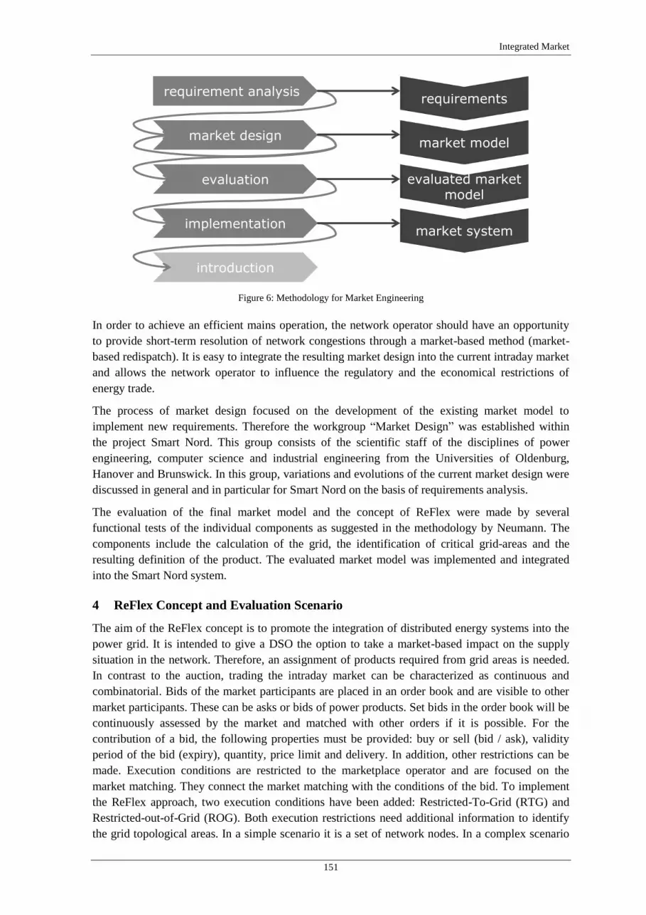
Integrated Market
151
Figure 6: Methodology for Market Engineering
In order to achieve an efficient mains operation, the network operator should have an opportunity
to provide short-term resolution of network congestions through a market-based method (market-
based redispatch). It is easy to integrate the resulting market design into the current intraday market
and allows the network operator to influence the regulatory and the economical restrictions of
energy trade.
The process of market design focused on the development of the existing market model to
implement new requirements. Therefore the workgroup “Market Design” was established within
the project Smart Nord. This group consists of the scientific staff of the disciplines of power
engineering, computer science and industrial engineering from the Universities of Oldenburg,
Hanover and Brunswick. In this group, variations and evolutions of the current market design were
discussed in general and in particular for Smart Nord on the basis of requirements analysis.
The evaluation of the final market model and the concept of ReFlex were made by several
functional tests of the individual components as suggested in the methodology by Neumann. The
components include the calculation of the grid, the identification of critical grid-areas and the
resulting definition of the product. The evaluated market model was implemented and integrated
into the Smart Nord system.
4 ReFlex Concept and Evaluation Scenario
The aim of the ReFlex concept is to promote the integration of distributed energy systems into the
power grid. It is intended to give a DSO the option to take a market-based impact on the supply
situation in the network. Therefore, an assignment of products required from grid areas is needed.
In contrast to the auction, trading the intraday market can be characterized as continuous and
combinatorial. Bids of the market participants are placed in an order book and are visible to other
market participants. These can be asks or bids of power products. Set bids in the order book will be
continuously assessed by the market and matched with other orders if it is possible. For the
contribution of a bid, the following properties must be provided: buy or sell (bid / ask), validity
period of the bid (expiry), quantity, price limit and delivery. In addition, other restrictions can be
made. Execution conditions are restricted to the marketplace operator and are focused on the
market matching. They connect the market matching with the conditions of the bid. To implement
the ReFlex approach, two execution conditions have been added: Restricted-To-Grid (RTG) and
Restricted-out-of-Grid (ROG). Both execution restrictions need additional information to identify
the grid topological areas. In a simple scenario it is a set of network nodes. In a complex scenario
market design
requirement analysis
evaluation
implementation
introduction
evaluated marketmodel
market system
market model
requirements

Smart Nord Final Report
152
area of a power grid, the utilization of appropriate keys is preferred. The execution conditions RTG
and ROG allow a market matching only for offers that are within (RTG) or outside (ROG) of the
defined grid topological area. With these design conditions it is possible to set bids in the intraday
market as a network operator which have a grid topological reference. A network operator is able
to set specific products in the market that counteract capacity congestions within the power supply.
The network operator is able to perform a redispatch within the distribution network while using
this product. For this reason two AND-linked bids need to be set in the market: the first bid (RTG)
to resolve the capacity congestion in the distribution grid itself and the second bid (ROG) for the
balance sheet of the first bid. Therefore the financial balance does not counteract against the
redispatch measure, the second bid should be located within the inverse grid area of the first bid.
The timing of the scenarios for evaluation is as follows: At first the units trade energy at the Day-
Ahead Auction of the Epex Spot market. On the basis of the trading results the unit schedules are
generated and transmitted to the DSO. Then the DSO performs a network state estimation of the
distribution grid and identifies possible capacity congestions within the electrical network.
Thereupon the DSO discovers the electrical grid zone (RTG) and defines corresponding ReFlex
products that are able to counteract on the capacity congestion. The corresponding ReFlex product
for the balance sheet (ROG) is also set up and both products are set on the intraday continuous
market with an AND-link. After the intraday trading, the DSO again can estimate a network state
estimation for the distribution grid with updated unit schedules and can take further action if the
capacity congestion was not solved completely.
The evaluation scenario includes one medium voltage grid with 71 underlain low-voltage grid that
contains 7808 grid nodes. It also includes 11,951 households, 789 heat pumps, 122 cogeneration
plants, 1048 photovoltaic modules and 30 wind turbines. Models of white goods (fridges/freezer)
as well as models of electric cars at first were an integral part of the evaluation scenario but had to
be removed due to hardware limitations of the simulation server.
5 Main Results
The main results are split into results of the simulation and general results. The following section
describes the simulation model and its results at first and ends with the general outcomes.
For the used simulation models, statistical parameters were calculated and visualized in the
behaviour diagrams. In each case, a power plant capacity of five units per simulation model has
been simulated over the year. The combined heat and power plant (CHP) is used in this section as
an example to describe the simulation model. Figure 7 shows a differentiated analysis of day
profile of a CHP within five diagrams. The diagrams show the daytime for one day with 1440
minutes on the horizontal axis and the power in watts on the vertical axis. The curves shown
represent the electrical power (blue), the thermal power (green) and the thermal demand (red) of
the unit. The first diagram “average day profile” shows the yearly average value for every minute
as a characteristic curve. The red curve clearly figures the daily rhythm of the thermal demand,
which is characterized by a high rise in the morning and by a peak in the evening and relative low
demand during the night. The thermal power of the CHP (green curve) follows the run of the red
line very well in the average. Deviations between the red and green curve can be explained by the
thermal maximum power of the CHP and by taking advantage of the thermal buffer memory. The
average value shows that the thermal buffer is loaded during the night time by the operation of the
CHP, because the green curve is largely above the red curve. The peak of the thermal demand in
the morning and in the evening will be covered by the collaboration of thermal buffer memory and
peak load boiler, because the characteristic of the thermal power of the CHP is below the thermal
requirements. The course of the electric (blue) and thermal (green) performance is very similar,

Integrated Market
153
since these quantities are directly related. Ordinarily from minute 400 (equivalent to 6.40 clock) to
minute 1300 (equivalent to 21.40 clock) an increased average performance by the CHP is provided.
Figure 7: Differentiated analysis of day profile of a CHP
The simulation results of each day type were summed according to the advertised and successfully
traded energy quantities of ReFlex products of one day. This makes it possible to determine the
daily amount of energy, which was also picked up by the ReFlex concept from the grid. The
difference between the tendered amount of energy and the actually traded energy produced an
amount of energy, which threatened the state of the power system and has to be shut down. These
operating numbers will be compared and contrasted in Figure 8. For each day the percentage of
successfully traded amount of ReFlex bids is shown. The figure shows the results for typical days

Smart Nord Final Report
154
during the transition period between summer and winter in the first four bars, followed by four
winter-type days and two summer type days. The abbreviations mean the following (first
character): transition (Ü); winter (W); summer (S). The second character differentiates between
working days (W) and Sundays (S). The last character of the coverage means Clear (H) or Cloudy
(B).
Figure 8: Seasonal evaluation to the percentage share of traded reflex amounts of energy
The proportion of traded ReFlex bids is subject to a significant seasonal variation. During the
transition days, as well as during the summer days, a proportion up to 26 % of the advertised
performance was sold. During the winter days there was no significant success. One reason for
those negative results during the winter days is based on the simulation models used, which cover
up those flexibilities. Both simulation models (heat pump and CHP) consider flexibilities for
evaluation. For that reason, the results reflect flexibility potentials reduced during the winter
months, because both systems refer to the thermal requirement of a connected object as well as
they must cover up their primary demand.
Another significant criterion is whether the day is a weekday or Sunday / holiday. This is clearly
reflected in the transitional and summer-type days, because the percentage of the amount of traded
ReFlex energy is significantly less on Sundays / holidays than on working days. The differences
regarding the transition type days are about 8 % (ÜH) respectively about 25 % (ÜB). Even during
the summer type days a high difference about 16 % is given. The third criterion describes a cloudy
/ unclouded scenario, which does not give a concrete statement. For it seems not to be possible as
the proportion of successfully traded ReFlex energy levels do not correlate.
The evaluation of the results on an annual basis shows how the results strongly depend on the
flexibilities. The reduction of the flexible simulation models (white goods, electric cars) has a
significant negative effect on the quality of the results. The analysis of each type day shows a
frequently violation of the voltage band of the upper voltage band in the middle of the day, which
results into the intensive electricity from the PV. The flexible consumers (heat pumps) cannot work
against the violation of the voltage band, particularly not within the winter months. The reason
behind is the design of the heat pumps. They can rarely provide their connected objects during the
winter with thermal power. Therefore heat pumps will permanently be in operation on cold days
and have no flexibility to obtain additional power. The thermal demand of households for
preparation was rather insignificant on warm days, whereby the heat pumps cannot handle the
additional heat power from the charge of the operation of the PV. The other flexible units are the
Integrated Market
155
CHP, which are very similar to the thermal coupling to the supplied objects in their behavior.
During the summer, the low thermal requirement prevents the operation. During the winter, a
shutdown due to the high thermal demand of the supplying object is not possible. Overall, there are
some type days which produce an overload within the MV network. This leads to correspondingly
high ReFlex bids by the network agents.
The magnitude of the required compensation is currently so high that the units behind the gird
overload are not able to provide sufficient flexibility. The scenario was defined in this study as part
of the project Smart Nord. The simulation results of this work repeatedly show that for the MV
network line expansion is necessary.
By the following assumptions (the ReFlex reduced voltage band violations, reduced line overloads,
transformer overloads and also increased the capacity for integration of RES) in particular the
possibilities of the network operator have been restricted to resolve capacity congestions.
Moreover, the results represent the potential of the ReFlex concept, which can be used in
combination with other measures for the network operator to increase the capacity of the current
electricity networks for renewable energy. It became also evident in the simulations that a network
expansion in the MV network is required. The concept could not solve the network problems.
However, a network expansion in the distribution network would require 3-5 years what can lead to
voltage band violations and grid overloads. During the transitional period until this network
expansion, the concept has the opportunity to implement a forthcoming network expansion, or to
use the time to expand efficiently for the energy revolution.
6 Conclusion and Outlook
In this sub project a market-based approach for the development of flexibilities was engineered.
This approach can serve as another possibility for a power company to increase the renewable
energy integration of the electricity grid. For this purpose, new requirements for a market design
were identified within a requirements analysis:
The compensation of lost revenue from the renewable energy due to the isolation will not be
sustainable with the increasing development of renewable energy. The renewable power plants
have to be traded directly on the energy market to respond on the price signals.
A precondition for an effective input to the energy transition is the practical relevance and the
compatibility to the existing market design. Therefore only market models with a possible
transition of the current market design will be developed.
The simulation study has shown that the potential of operators’ flexibility through the ReFlex
concept can be utilized. These potentials are visible, especially in the transitional period.
Furthermore they are about 20 % of the tendered amount of energy in the simulation studies.
Localizable products are characterized by an additional condition of completion of a market
matching. This only allows trading on the market when the market participants are located in the
defined grid area of the DSO. Therefore only a slight change in the current market design is
necessary, what is reflected in an additional execution condition for intraday products. The
qualities of results based on the scenario, in particular due to the transition time by the use of
thermally coupled systems as the only flexibility option. The limitation of these systems depends
on the complexity of the simulation environment, the resulting computation time and the memory
requirements.
The ReFlex concept was not always capable to counteract grid problems within the simulation
study. This is due to the scenario, which is based on a network state in 2011 and covering the
development of renewable energy with a time horizon to 2030. Although it leads to significant

Smart Nord Final Report
156
reverse power flow in the medium voltage grid and associated overload. Within the illustrated scale
a grid expansion in the range of medium voltage network is not averted by the ReFlex approach.
The evaluation was based on the evaluation scenarios of the research project Smart Nord and with
mosaic-simulation framework which was developed at OFFIS. This market design of today's
energy market is modelled in the simulation framework and implemented enhancements are based
on the ReFlex concept.
Overall, the developed market model has a non-massive intervention to the existing market design.
It merely extends the existing market design to an additional execution condition for Intraday-
market products, so that a transition from the current market design to the proposed market model
is possible.

Integrated Market
157
Work Package 3.3: Business Models for Energy Producer and
Price Sensitive Consumer
Sören Christian Meyer46
, Hans-Jörg von Mettenheim46
and Michael H. Breitner46
1 Current Market Situation on the German Electricity Market
The German electricity market is divided into areas with strong market regulation and fixed taxes
and levies as well as market driven segments. Examples for market driven participants are large
scale fossil power plants and large scale electricity consumer.
Those fossil power plants actively base their production on EEX-market prices and as additional
revenue on auction based controlling power compensation. Assumed that the marginal cost (the
merit order) are price setting on both markets, a cost effective behaviour for effective and balancing
power supply can be assumed.
Large electricity consumer (above 1 GWh) profit as well from 85 %-99 % reduced EEG
apportionment (§64 EEG 2014) as from reduced grid tariffs due to their connection to the medium
or high voltage grid and options like the atypical grid usage. (§19 StromNev).
Figure 9: Tax and levy burden on electricity consumption in eurocent per kWh
In contrast small scale decentralized producer are either dependent on weather conditions (Wind,
PV) or on heat demand (CHP). For all three exist with the market premium model the option to
participate in the market, but the investment in steering infrastructure needs to be set in relation to
46
Leibniz Universität Hannover, 30167 Hanover, Germany,
[email protected], Institute for Information System Research

Smart Nord Final Report
158
the generation capacity. For large electricity customers the price is mainly based on fixed taxes and
levies, as well as administrative cost and margins. For those customers no incentives for grid
friendly usage change exist.
From the economic perspective, it is efficient, to supply grid services with lowest overall cost as
possible. As long as large scale electricity generator and consumer are able to supply these services
with low cost for steering infrastructure, this is indeed the best option.
With the Transformation of the Energy System (TES) and the substitution of centralized fossil
power plants by decentralized renewable power plants, grid services are no longer minor products
from effective power generation but have to be actively supplied by small, decentralized agents. In
general the decrease of steerable producing units already results in a higher volatility and
increasing price spread in the effective power market. With further progress of the TES and
decreasing costs of steerable units small customer and producer are going to have an incentive to
invest in measurements enabling them actively to benefit from volatile prices for effective and
balancing power.
Therefore in the long run the current high liquidity on the market for balancing power will decrease
resulting in an increase of the overall price level as well as the volatility of balancing power prices.
In consideration of a highly legislative regulated market and long investment live times in the
electricity sector, it is necessary to develop solutions in advance of the expected shortage.
2 Tax and Duty Burden on Electricity in Germany
Figure 9 illustrates that fixed taxes and levies are the main price component and solutions for
reducing this burden needs to be found first to create an economic feasible business model for
flexible pricing. The taxes add up to 17 eurocent per kWh. Most important factors are the EEG
apportionment with 6.24 eurocent per kWh and the grid fee (dependent on area) with an average of
5.87 eurocent per kWh. Connected to the grid usage is the concession levy, which differs
dependent on the city size, increasing for larger cities and having an average of 1.62 eurocent per
kWh. The energy tax of 2.05 eurocent per kWh is dependent on extracting electricity from the
public grid and the sales tax is an addition of 19 % on the electricity price and is also raised on the
taxes included in the electricity prices. Furthermore with such a tax burden the consumer price of
17 eurocent per kWh only for refinancing taxes and levies it is nearly impossible to develop
flexible electricity tariffs. Therefore the business model needs an essential step to reduce the tax
burden.
Due to the nature of the different taxes the grid fee can be saved if no public grid is used. If a
public grid is used, only the actual usage needs to be paid. Therefore the usage of only the low
voltage grid, saves the grid fees for high voltage usage. The EEG apportionment can be saved if
electricity from renewable sources is used by its proprietary and the maximum power is below
10 kWp. If the maximum power is above 10 kWp 40 % of the EEG apportionment has to be paid.
Furthermore the power generation units have to be in the same low voltage grid. The grid fee is
dependent on the usage of a low voltage grid, therefore it has to be paid if electricity is transported
from one household to another. The assessment basis of the electricity tax is the usage of power
from the public grid, but can be avoided if the electricity is used in direct local connection to its
generation. The sales tax can only be reduced if other taxes and levies are reduced.
3 Future Renewable Electricity Generation Cost
The second essential part for future business models is the knowledge about the development of
renewable electricity prime cost. Therefore production based experience curves were used, due to

Integrated Market
159
the fact that they have proven to be robust for long time price predictions and they are widely used
in policy scenarios. Experience curves are based on statistical derived learning rates. Learning rates
describe the percentaged price decrease of a product, each time the amount ever produced is
doubled. Learning rates are statistical derived from market data.
The learning rates were retrieved from a literature review of 100 scientific high ranked paper
dealing with the research area. This data were combined with market forecasts from the IEA. Those
predictions can be included in cost calculations. The shown prices are examples for the conditions
in the Hanover region. The resulting experience curves are shown in Figure 10. The forecast shows
that for onshore wind energy a further price decrease by 50 % can be expected and electricity from
photovoltaic rooftop installations can reach price levels of 7.5 eurocents per kWh until 2030.
Figure 10: Expericene curve based prediction of renewable electricity generation cost per kWh
4 Description of the Developed Business Model
The business model was designed as iterative process using the methodology of Wirtz [2] and
combined with design science research. The resulting business model was simulated with the
environment “MATLAB” and the result was used to optimize the business model which was finally
tested in the simulation.
The developed business model combines the described tax and duty burden criteria with the price
forecasts. As result mainly for the EEG apportionment and the grid fee a “Customer Installation”
would be the most inclusive solution. Using a construct consisting of an energy association as
owner of the installation and customer being member in the association [5].47
The needs for the a
customer installation as actually being owned by the association as well as the untypical grid
topology with wind power and free field-PV connected to the distribution grid mainly limits the
business model to newly developed area. Furthermore the economic feasibility of CHP is better if
the heat distribution network can be built together with for example the water supply.
47
The author wishes to appoint to unsettled lawsuits in close relation to the legal construct. For use in actual
projects waiting for a cleared legal situation after settlement of those trials is advised.

Smart Nord Final Report
160
The project calculation is based on a fictive example project with 86 accommodation units
distributed in mixed apartment and detached houses.
For keeping the amount of other supplier minimal, it is necessary to offer electricity with a cost
competitive pricing. In the Hanover region the reference price for an renewable electricity supplier
is a value added tax cleared net price of 19.6 eurocent per kWh and an annual base price of 68 €.
Figure 11: Schematic diagram of the consumer installation
The needed IT infrastructure for optimization and billing can be used as hosted solution priced with
3250 € p.a. or about 40 € p.a. per customer. The overall electricity consumption from the public
grid or feed in into it from the customer installation is measured by the sum counter model.
Therefore the electricity demand or feed in at the connection point to the public grid, the power
generation within customer installation, and the electricity consumption of all customer is
measured using a 15 min resolution. This is necessary, for being able to subtract customer within
the customer installation, receiving electricity from other suppliers and deliver by calculation
electricity from the public grid. This additional effort is needed, due to the regulatory necessity to
allow the customer to choose their supplier without restriction. Furthermore a smart meter is
obligatory for flexible electricity tariffs resulting in investment related cost of about 18 €.
Therefore the net pricing is sufficient for maintaining the optimization and data collection
infrastructure.
Hence the competitive average price of 19.3 eurocent per kWh needs to cover the remaining tax
and levy burden, the consumer installation, the generation cost and the producer and consumer
incentive for grid stabilizing demand shift.
The electricity generated and carried within the customer installation is freed of 60 % EEG
apportionment, grid fees and electricity tax. The resulting subsystem therefore only needs to pay
2.5 eurocent per kWh EEG apportionment, 1.79 eurocent per kWh concessions levy if public

Integrated Market
161
ground is crossed and the value added tax of 19 % on the overall price. For the residual load from
the public grid a peak load based basic charge needs to be paid. The customer installation can be
financed by about 3.5 eurocents. With 11.71 eurocent as remaining factor, the most suitable
electricity sources are gas powered CHP with electricity generation after CHP-subsidies (5.41
eurocent) or wind power in the same price range. Simulations have shown the option to allow a
price range low to high about 18-28 Eurocent. Therefore the administrative cost needs to remain
about 2 eurocent per kWh or 8000 € for the subsystem. This is only possible if the billing takes
place automated and in relatively large scale. So either the administration has to take place for a
larger group of customer installations or by a service supplier.
In 2030 as described a higher volatility of the electricity prices can be assumed. Those lower
renewable electricity prices and higher price fluctuations as well as existents of smart metering
increases the cost competitiveness of the customer installation. Furthermore in general fixed
electricity prices might vanish, due to those higher price fluctuations and the existents of smart
meter. Also the existence of smart home components might progress driven by additional
functionality if hardware can be controlled by smartphones. Under those conditions combined with
lower prices the simulation was able to economically run a self-balancing system shown in
Figure 11. It consists of batteries, electric vehicles, wash-dryer as steerable consumer and the
central CHP-Unit as steerable supplier. As non-steerable the residual household load and wind
power and PV is used.
Figure 12: Interaction between the business model components
Figure 12 illustrates the modular business model. In the best case scenario heating and electricity
are automatically billed together with smart metering and smart heat counter. The collected data
can be used as well for billing as for forecasting purposes. The optimization server optimises the
CHP-scheduling based on weather prognosis. This can be done in a local solution aiming to reach
self-sufficiency, or optimized for benefit from high price timeslots on the EEX thereby smoothing
the electricity prices. When economic feasible, Smart-Home solutions are able to use price signals

Smart Nord Final Report
162
for steering of the household units. Large consumption units in households like EV or air
conditioning in commercial units can be directly controlled by the optimisation server. The four
segments of the holistic approach are interconnected and reach the maximum efficiency when
joined. Due to the long lifetimes of the related goods and infrastructure of 15-40 years the approach
was developed to be able to work with partial solutions. For example is the CHP unit joint with its
billing infrastructure is already today available and in the described newly developed area scenario
economic feasible. It can be run grid stabilizing and is flexible enough to smooth supply and
demand peaks on an hourly base. With the direct marketing model sufficient market incentives for
this steering exists. From the technological perspective it can also contribute minute grid reserve
capacities which will become attractive if those is lesser contributed by large fossil power plants.
Furthermore the CHP in the solution is able to contribute a significant CO2 reduction compared
with a solutions based on local gas powered heating.
Overall the sub-project was able to show, that at least in the 2030 scenario VPP solutions combined
with Smart-Home components are able and economic feasible to actively contribute grid services,
secured power and controlling power compensation. Furthermore it can reduce the volatility in
EEX-electricity prices. Thereby VPP are able to fill part of the gap left by the reduction of large
fossil power plants. The sub-project was able to show, that if enough steerable consumer exist, a
price based supply-demand balancing is economic feasible in newly developed areas and can be
combined with CHP. The legislative situation thereby forces difficult solutions. It would be
preferable and lead to less market distortion, if the amount based tax and levy burden was changed
towards a price based percentual system. This would allow to give easier price incentives also to
non-privileged small commercial and private customers.
References
[1] N. G. A. Hemdan, F. Muuß, D. Unger, M. Kurrat, “Reactive Power as an Ancillary Service Provision
into Transmission Networks through Decentralized Generation,” Cigre Belgium 2914.
[2] M. Kurrat, N. G. A. Hemdan, B. Engel, R. Canders, M Henke, “Technical challenges for ancillary
services provided by decentralized power generation in active distribution systems,” ETG Kongress
Berlin 2013
[3] F. Muuß, N. G. A. Hemdan, M. Kurrat, D. Unger, B. Engel, “Dynamic Virtual Reactive Power Plant
in Active Distribution Networks,” Powertec, Eindhoven 2015
[4] D. Neumann, “Market Engineering - A Structured Design Process for Electronic Markets Faculty of
Economics Karlsruhe,” University of Karlsruhe (TH), 2004.
[5] B. W. Wirtz, “Business Model Management : Design - Instrumente - Erfolgsfaktoren von
Geschäftsmodellen,” 3. akt. u. überarb. Aufl. 2013. Wiesbaden: Gabler Verlag, 2013.
[6] C. Köpp, H.-J. von Mettenheim, M. H. Breitner, “Decision Analytics mit Heatmap-Visualisierung von
mehrschrittigen Ensembledaten.” Wirtschaftsinformatik: 147. doi:10.1007/s11576-014-0417-3., 2014.
[7] B. Küster, A. Koukal, M. H. Breitner, “Towards an Allocation of Revenues in Virtual Clusters within
Smart Grids” IWI Diskussionsbeiträge 60 (September), 2013.
[8] S. C. Meyer, M. H. Breitner, “Electricity Associations as Marked - Based Steering Mechanism and
Alternative to Fixed Feed - in Tariffs,” Proceedings of the 28th EnviroInfo 2014 Conference: 729–
734, 2014.


Distribution and Transmission System
165
Sub-Project Four:
Distribution and Transmission System


Distribution and Transmission System
167
Overview on Sub-Project Four:
Distribution and Transmission System
Lutz Hofmann48
, Timo Breithaupt48
, Steffen Garske48
, Torsten Rendel48
,
Bernd Engel49
, Stefanie Koch49
and Marco Zobel50
1 Introduction
Within the ongoing transformation of the electric energy supply system several questions of grid
integration and overall system stability occur. With the decreasing feed-in of conventional thermal
power plants, the ancillary services formerly provided by conventional power plants have to be
taken over by distributed generation (DG) mainly using renewable energy sources (RES). For
future energy supply systems, the possibilities and the boundaries of power system states with a
high share of DG units, which – in opposite of the conventional generation – are connected to the
distribution grid have to be analysed. Hence this is a matter of transmission and distribution grids,
both system levels have to be analysed in one integrated simulation model. Therefore an overall
system model is developed to evaluate the two evaluation scenarios of this research project – the
reference scenario 2011 and the future outlook scenario 2030. The integration of DG units within
these scenarios into the distribution grid as well as micro combined heat and power (CHP) units in
particular are analysed in detail within this sub-project.
The research questions of this sub-project cover the provision of two essential ancillary services.
These are reactive power provision to support stationary voltage stability in all voltage levels and
provision of control reserve to ensure frequency stability. The reactive power provision is managed
within the integrated grid and market simulation model (INES) to secure valid power system states.
The frequency stability studies are done for characteristic points in time based on characteristic
system states and incidents. In this way the need and the amount of primary control reserve
provided by DG units are determined. Furthermore the possible capabilities and also the limitations
of grid states with high shares of DG can be analysed and evaluated. This is accompanied with
simulations and laboratory experiments of micro-CHP systems and detailed analyses of the grid
integration of DG within the medium and low-voltage distribution grid.
2 Goals
The main goals of the sub-project four: Distribution and Transmission System are:
Setting up a system model for integrated simulations of transmission and distribution grid
(work package 4.1) based on the integrated grid and market simulation
Integration of the evaluation scenarios 2011 and 2030 into the system model
(work package 4.1)
Simulations of the evaluation scenarios 2011 and 2030 in the system model and the distribution
grids (work package 4.1 and 4.2)
Analyses of stationary system states and provision of reactive power by DG units in the
underlying voltage levels to the transmission system (work package 4.1)
48
Leibniz Universität Hannover 49
Technische Universität Braunschweig 50
EWE-Forschungszentrum für Energietechnologie e.V.

Smart Nord Final Report
168
Frequency stability studies within the system model for characteristic points in time to
determine the required provision of primary control reserve by DG (work package 4.1)
Evaluating the supply of active power using micro-CHP systems (work package 4.2)
Assessment of the integration of DG units in the medium and low-voltage distribution grid
(work package 4.2)
3 Main results
The work package 4.1 developed an overall system model as extension of the integrated grid and
market simulation model in cooperation with the work package 4.2 and the work group Scenario
Design. This system model is suitable for simulations of stationary power system states and for
frequency stability studies within the evaluation scenarios 2011 and 2030 of this research project.
The provision of reactive power by DG units was evaluated for different reactive power
management approaches. The frequency stability studies were done for four characteristic points in
time based on an incident referring to the ENSTO-E reference incident. The simulations show that
a secure system operation regarding frequency stability in the future scenario is possible and that
within the simulation model the provision and management of reactive power is essential. To
ensure stable operation, RES generation has to participate in a fastened primary control at some
points in time.
Furthermore it was shown that the ongoing installation of DG units leads to a high grid
reinforcement demand. Within the evaluation scenarios for the distribution grid section and the
increased amount of DG a reinforcement of 32 % of all cables and 58 % of all transformers at the
MV-level was needed. Similarly, at the LV-level 11 % of the cables and 7 % of the transformers
had to be supplanted. It was shown that the simulated and measured data of the micro-CHP within
laboratory validations are consistent. The evaluated CHP system matches the requirements for a
controlled active power supply, but its high potential can only be used if a high number of systems
are installed in the local grid.

Distribution and Transmission System
169
Work Package 4.1: Interconnected System
Timo Breithaupt51
, Steffen Garske51
, Torsten Rendel51
and Lutz Hofmann51
Abstract
The ongoing transformation of the energy supply system from a classical design with large scale fossil power
plants and power flows directed from ultra-high voltage to low voltage levels to a generation mainly realised
using renewable energy sources (RES) leads to several questions of grid integration and overall system
stability. Conventional thermal power plants are more and more displaced by distributed RES generation
which is mainly connected to the distribution grid. With this changed power plant dispatch the ancillary
services formerly provided by conventional power plants have to be taken over by RES generation. As the
provision of ancillary services is a matter of overall system stability within the transmission system, not only
the possibilities, but also the boundaries of future energy supply systems with a high share of RES generation
have to be analysed. Since this topic is a matter of both, transmission and distribution grid, a system model
has been developed to analyse both system levels. These analyses have been done for a reference and a future
outlook scenario developed within this project. The system model comprises the European electricity
wholesale markets, the Continental European Transmission grid and single distribution grid sections
modelled in detail at selected transmission grid nodes. By means of this system model mainly two ancillary
services have been investigated: reactive power provision to support stationary voltage stability and control
reserve provision to ensure frequency stability. The reactive power provision is analysed in both scenarios
and implemented as new optimisation approaches for the transmission system model as well as the extended
model with underlying distribution grid sections. The provision of reactive power has been analysed within
the voltage bands deviations of the transmission system model. Several approaches have been examined to
attain valid and stable system states and to quantify the reactive power exchange between the two system
levels. The frequency stability studies show, that a secure system operation regarding frequency stability in
the future scenario is possible. To ensure this stable operation, RES generation has to participate in a fastened
primary control at some points in time.
1 Introduction
The analysis of the contribution of underlying voltage levels for ancillary services to the
transmission system is a matter of both distribution and transmission grid. Hence, both system
levels have to be evaluated in one overall system model. A detailed model of the ENTSO-E52
Continental Europe transmission system (see Figure 1) is given by an integrated grid and power
market simulation (INES) developed by the Institute of Electric Power Systems (IEH) [1] [2] [3].
≥ 750 kV
380 kV - 750 kV
300 kV - 380 kV
220 kV - 300 kV
< 220 kV
HGÜ
Figure 1: Integrated grid and power market simulation
51
Leibniz Universität Hannover, 30167 Hanover, Germany,
[email protected], Institute of Electric Power Systems 52
European Network of Transmission System Operators for Electricity, https://www.entsoe.eu/

Smart Nord Final Report
170
The INES system model is parametrised on basis of several databases, e.g. power plant allocation,
regional characteristics as well as various input parameters like e.g. grid and economic data. With
this simulation environment a wide foundation for different analysis of stationary processes like
transnational transmission grid calculations is given and a fundamental data basis can be used for
this project.
The answering of the research questions of the work package (WP) 4.1 are based on the analyses of
stationary as well as dynamic processes (see Figure 2) carried out by example of the two evaluation
scenarios which were prepared by the work group Scenario Design (see report of the Work Group
Scenario Design) for this research project. Firstly, the year 2011 (reference) and secondly, the year
2030 (future outlook) have been implemented into the simulation model and have been evaluated
and compared in respect to stationary system state and frequency stability. With this methodology
the need and the amount of contribution of distributed generation (DG) units, which basically use
renewable energy sources (RES), to ancillary services, esp. provision of reactive power and control
reserve, in the transmission system can be analysed and estimated.
Stationary ProcessesIntegrated grid and
market simulationDynamic Processes
- Transmission grid
- Distribution grid
- Scenarios 2011/2030
Stationary system
state
Characteristic points
in time
- Power plant dispatch
- Load flow calculations
Frequency stability
analysis
Figure 2: Methodology of the work package 4.1
Therefore the WP 4.1 in cooperation with the WP 4.2 and the work group Scenario Design has
developed an integrated system model as extension of the INES simulation environment covering
all voltage levels with coherent growth forecasts for power generation in both scenarios. This can
be used for the analysis of stationary processes (see chapter 3) and with extensions made within
this project also for the evaluation of frequency stability (see chapter 4).
2 Overall System Model
Because of the spatial expanse of the ENTSO-E transmission system and the expanse of
distribution grids from the ultra-high voltage (UHV) to high voltage (HV) transformation down to
the single households in the low voltage (LV)-level a simulation of the entire transmission system
with all underlying voltage levels is not feasible. Thus only at single UHV nodes a distribution grid
section is integrated into the INES simulation framework of the transmission system. Hence, as
presented in [4], one challenge was to integrate the underlying voltage levels with detailed grid,
load and generation data (see work group Scenario Design) for the medium voltage (MV) and LV
level into the existing system model of the transmission grid. Therefore, the UHV nodal load and
generation data was partitioned in distributed models of high voltage and medium voltage load and
decentralised generation. Herewith the given aggregated data of one UHV node was substituted
with an equivalent share of the underlying voltage levels and with a coherent consideration of the
two scenarios for the years 2011 and 2030 in one system model. The HV level is modelled with

Distribution and Transmission System
171
synthetic grids for each considered UHV node similar to the MV grid, which is based on a common
MV benchmark grid [6]. For further description please refer to [4] and the report of the work group
Scenario Design.
With this approach it is possible to analyse the two evaluation scenarios of the research project
Smart Nord for both transmission and distribution grids in one coherent and detailed simulation
framework and to determine the contribution of underlying voltage levels to ancillary services for
the transmission system.
3 Analyses of Stationary Power System States
3.1 Power Plant Dispatch and Market Simulation
As a first result of the simulation of the overall power system using the integrated power system
and power market model INES a power plant dispatch is determined with a market simulation
based on a merit order of marginal costs, including the priority feed-in of RES with zero marginal
costs [8]. Depending on the current load, which is partitioned in discrete load blocks (see [2]), all
available power plants are arranged according to their current marginal costs
𝐶m =𝐶fu
𝜂el+
𝐶CO2
𝜂el𝐸𝐹 +
𝑡su
𝑡op(𝐶fu
𝜂el+
𝐶CO2
𝜂el𝐸𝐹) (1 − e−
𝑡down𝜏 ) (1)
which leads to a load and time depending power plant dispatch (see Figure 3 for the scenarios 2011
and 2030 for the German transmission system within the INES simulation model).
solar
wind
hydro
further
oil & gas
hard coal
lignite
nuclear
Figure 3: Power plant dispatch in the simulation model for two weeks in January in the scenarios 2011 and 2030
In the scenario 2011 (left figure in Figure 3) with two weeks of high load in January), the base load
is mainly provided by nuclear and coal-fired power plants while the share of DG fluctuates
between 5 GW and 20 GW. In comparison with the scenario 2030 (right figure in Figure 3 with
two weeks of high load in January) including the withdrawal from the nuclear energy programme, a
high ratio of the energy is provided by the RES (in this case mainly wind energy generation), which
is mostly complemented in times of peak load or low wind generation with coal-fired or gas-fired
power plants. These results for the power plant dispatch, generation by RES and load time series
are the input data for the subsequent power system calculations.
3.2 Load Flow Calculations and Grid Expansion
The simulation environment INES combines the power plant dispatch for the different scenarios
with geographical generation and grid data, which allows load flow calculations [11] for the
transmission grid model. Including all electrical equipment models, current load and generation
data regarding to the power plant dispatch and further input parameters such as high-voltage-direct-
0 100 200 3000
20
40
60
80
time in h/4
activ
e p
ow
er
in M
W
0 100 200 3000
20
40
60
80
time in h/4
activ
e p
ow
er
in M
W

Smart Nord Final Report
172
current (HVDC)-transmission or inter transmission system operator transit data for all utilities
within the simulation model the grid equation is compiled as
3𝑼N𝒀𝐍𝐍∗ 𝒖𝐍
∗ − 𝒔N(𝒖N) = ∆𝒔N(𝒙) (2)
This equation is separated in a real and an imaginary part and approximated by a Taylor
expansion [2] with
𝜕∆𝒑(𝒙𝒗)
𝜕𝒙𝐓 𝒙𝒗+𝟏 = −∆𝒑(𝒙𝒗) (3)
𝜕∆𝒒(𝒙𝒗)
𝜕𝒙𝐓 𝒙𝒗+𝟏 = −∆𝒒(𝒙𝒗) (4)
The equations (3) and (4) can be summarised with the Jacobi-Matrix which depends on the choice
of the state vector, where Cartesian and Polar coordinates are possible. For further description
especially for the implementation within the INES simulation model please refer to [11] [8] [2] and
[3].
Because of the extensive transformation of the energy supply system with the scenario 2030 the
transmission grid model of the reference scenario 2011 used in the simulation framework is not
sufficiently dimensioned (see Figure 4). Thus, the expansion of the transmission grid had to be
considered in the transmission system model (cf. work group Scenario Design report). This was
realised by implementing the concluded grid expansion projects from the ENTSO-E ten years
network development plan (TYNDP) [6] and the German Netzentwicklungsplan (NEP) 2012 [22].
6 8 10 12 14 16
47
48
49
50
51
52
53
54
55
56
0
0.02
0.04
0.06
0.08
0.1 1,0
0,8
0,6
0,4
0,2
0
Figure 4: Load flow analysis of the transmission system with the average load of all power lines
in relation to nominal load in the scenarios 2011 and 2030 (January)
These plans cover an outlook of transmission grid expansion for the next ten years and are
implemented into the transmission system model. Hence, these plans do not cover the total growth
forecast up to the year 2030, the further need of grid expansion is integrated into the grid models
based on load flow analyses. This led to a high amount of additional grid expansion measures. This
can be attributed firstly to the gap of ten years in the official grid expansion plans and secondly to
the growth forecast of the power plant distribution. This forecast was modelled with an algorithm
to allocate the power plants for the year 2030 which is based on the data of the simulation model of
the year 2011 and not on actual future forecasts for each single power plant (see Work Group
Scenario Design). With varied load flow analyses all affected power lines have been improved to
secure a valid system state.
6 8 10 12 14 16
48
50
52
54
56
6 8 10 12 14 16
48
50
52
54
56

Distribution and Transmission System
173
3.3 Voltage Bands and Reactive Power Management
In addition to the load flows on all power lines, one main challenge within the stationary system
model and simulations for both scenarios has been the compliance of the node voltages to the
voltage bands and therefore the reactive power management in the transmission system simulation.
Depending on regional grid connection and allocation of power plants, DG and their feed-in of
active and reactive power, the voltage bands differ widely in the grid model (see Figure 5).
6 8 10 12 14 16
47
48
49
50
51
52
53
54
55
56
0
0.02
0.04
0.06
0.08
0.110 %
8 %
6 %
4 %
2 %
0 %
Figure 5: Average voltage band deviation in relation to nominal voltage in the transmission system model with and
without reactive power management
In the INES model within the reference scenario 2011 the DG units originally feed in with a power
factor of cos(𝜑) = 1. This would lead to extensive voltage band violations and a high need of
reactive power provision of remaining generation units or reactive power compensation in
simulations of the scenario 2030. Stationary reactive power compensations are currently not
considered as asset data within this simulation model and the high share of DG units would not
provide the required reactive power. Hence, a reactive power management was developed to ensure
the voltage bands for each node and a reasonable distribution of reactive power for both
conventional power plants and DG within their operation boundaries. As a first approach to
generate a valid system state, this optimisation identifies in several iterations all violations of
voltage bands and reactive power boundaries by setting the nodal reactive power or the node
voltage to its maximum allowed value. Afterwards a load flow calculation is executed and the
optimisation is executed as long as violations of voltage bands or reactive power boundaries are
identified. Thus all node voltages are optimised in order of their grade of voltage band violation to
ensure a reliable system state in all calculations (see Figure 5).
3.4 Reactive Power Provision of Underlying Voltage Levels
In this context one main research question was the contribution of underlying voltage levels to the
provision of ancillary services like e.g. reactive power provision. Thus, in several scenarios the
provision of reactive power by DG units located in the HV and MV level was analysed with the
overall system model including the distribution grid sections at different single UHV nodes. For a
fundamental estimation of the range of possible reactive power contribution, a basic optimisation
was developed to identify the range of reactive power demand within the transmission grid model.
For one node with a high share of DG the nodal data was substituted with a distribution grid
section. As a first approach the usage of discrete inductive or capacitive power factors for the
distributed generation units (wind and solar)
cos(𝜑) = cos(𝜑ind) ∀ 𝑢K > 𝑢K,r
cos(𝜑kap) ∀ 𝑢K < 𝑢K,r (5)

Smart Nord Final Report
174
in dependence on upward and downward voltage band violations was used to quantify the reactive
power demand of the transmission grid model. In this way the dependence of the reactive power
provision on the current active power contribution within the distributed DG units in the
distribution grid section (see diagram on the left side in Figure 6) can be analysed.
Figure 6: Reactive power optimisation and the corresponding nodal voltage
The node voltage calculated for the reference scenario 2011 for a node with a high share of DG in
the node region could be improved up to several kV depending on the overall grid state. With the
time depending contribution of the RES, the overall power plant dispatch fluctuates time-dependent
and consequently the overall grid state of nodal voltages and load flows. This leads to diverging
feasibility for voltage optimisation of the reactive power contribution of the DG in the distribution
grid section due to the diversity of the transmission grid model states. With the use of discrete
power factors the demanded range of reactive power provision can be quantified for single UHV
nodes. Hence, this methodology is only suitable for single UHV-nodes, a reactive power
management for the overall transmission grid is required for an optimisation of the entire system.
Based on [7] an optimisation approach was implemented to minimise the deviation of all node
voltages in relation to reference voltages for each UHV node. In this way the reactive power
demand and the potential of voltage optimisation for the entire grid model can be analysed.
Without reliable reference voltages for all nodes as a first approach all voltages were optimised in
reference to their nominal voltage. From the Jacobian matrix of the Newton-Raphson-method in
polar coordinates
[
𝜕∆𝑝
𝜕∆𝛿
𝜕∆𝑝
𝜕∆𝑢𝜕∆𝑞
𝜕∆𝛿
𝜕∆𝑞
𝜕∆𝑢
] [∆𝛿∆𝑢
] = − [∆𝑝∆𝑞
] (6)
the correlation of voltage alterations regarding reactive power variations can be received through
inverting as
[∆𝛿∆𝑢
] = −[
𝜕∆𝛿
𝜕∆𝑝
𝜕∆𝛿
𝜕∆𝑞
𝜕∆𝑢
𝜕∆𝑝
𝜕∆𝑢
𝜕∆𝑞
] [∆𝑝∆𝑞
] (7)
-400 -200 0 200-100
-50
0
50
100
150
200
250
active power in MW
reacti
ve p
ow
er
in M
var
400 450 500412
414
416
418
420
422
424
time in h/4
no
dal
vo
ltag
e i
n k
V

Distribution and Transmission System
175
which is valid for minor changes of the operating point. The requested coherence of nodal voltage
and reactive power provision results in
[∆𝑢] = − [𝜕∆𝑢
𝜕∆𝑞] = −[𝑉][∆𝑞] (8)
With the parameters of the integrated grid and market simulation for each operating point
aggregated reactive power constraints for each node can be determined in dependence of current
provision of DG units (maximum and minimum power factor), generator power limits and voltage
bands. The minimum deviations can be solved with the Gauss-Newton-algorithm [7] to calculate
the optimal reactive power ∆𝑞red of all nodes which can provide reactive power. After this
optimisation load flow calculations with the optimised voltages as new reference voltages and the
resulting reactive power provision are performed within iterative optimisations, because the results
depend on the operating point [7]. The results of this optimisation can be used to analyse the
regional reactive power demand and the overall potential of reactive power provision of the
underlying voltage levels within the transmission system model and as an approach to gain valid
system states (Figure 7). The calculated demand and the possible provision are time dependent and
differ strongly within the INES model. These facts complicate a summarising evaluation, especially
because of the size and calculation time of the simulation environment.
6 8 10 12 14 16
47
48
49
50
51
52
53
54
55
56
0
0.02
0.04
0.06
0.08
0.110 %
8 %
6 %
4 %
2 %
0 %
Figure 7: Average node voltages in the transmission system model with and without minimisation of
voltage band deviations
For further analyses with this approach reliable reference voltages are needed and stationary
reactive power compensators should be included within the grid model to improve the results of the
reactive power management approaches in the simulation model. This approach is used as
optimisation after the “standard” load flow calculation of the INES model. Further research is
needed for a reactive power optimisation integrated within the INES model and load flow
calculations. Main challenges for the analyses of stationary system states have been the
implementation of the future outlook scenario 2030 and the determination of valid system states,
which could not be realised for all points in time. This can be attributed to various challenges
within the architecture of the INES model in combination with the key data of the scenario 2030, as
e.g. the uncertain forecasts data (grid expansion and future power plants allocation).
The transfer project “iQ-Regler”53
will develop further approaches to analyse the reactive power
contribution of underlying voltage levels in more detailed scenarios and the results of the reactive
power adjusting ranges can be used within the transfer project.
53
http://smartnord.de/downloads/Praesentationen_Abschlusstagung/iQ-Regler.pdf

Smart Nord Final Report
176
4 Frequency Stability Studies
In order to carry out frequency stability studies, the stationary system model described above is
extended. Regarding the time frame of the relevant transient phenomena a quasi-stationary
approach is chosen: grid, load, decentralised generation, primary control and stators of synchronous
machines are described with algebraic equations using phasors while rotors, motion, excitation
systems and power system stabilisers of synchronous machines as well as secondary control are
depicted by state space equations. The system is calculated by solving the state space differential
equations with numerical integration using the classical Runge-Kutta method and the algebraic
equations by turns every integration time step [13]. The start values of the state variables are
calculated from the results of the market and load flow simulation (see chapter 3).
As the resulting model and thus the calculations are very extensive and time-consuming, it is
common practice to identify single points in time with characteristic properties and to analyse them
in detail. In the past, these characteristic points in time have been times of low load and therefore
low generation of conventional power plants. As conventional power plants provide most of the
inertia which decelerates the frequency deviation resulting from a difference between load and
generation, these points in time had the highest dynamic frequency drop. To regard the
displacement of conventional generation with its inertia by RES dominated DG, four characteristic
points in time are identified: high load/high DG; high load/low DG; low load/high DG; low
load/low DG. These four points in time are simulated in detail for the scenario 2030 and are then
compared to the corresponding points in time of the reference scenario 2011.
4.1 Grid and Load Modelling
The chosen quasi-stationary approach neglects transients in grid and stator windings of generators.
This allows a representation of grid and stator voltage with phasors for steady-state relationships.
Basis is the standard grid equation
𝒀𝐍𝐍𝒖𝐍 = 𝒊𝐍 = 𝒊𝐆 + 𝒊𝐃𝐞𝐳 + 𝒊𝐋 (9)
where 𝒀𝐍𝐍 is the complex node-admittance matrix, 𝒖𝐍 the vector of complex node voltages and 𝒊𝐍
the vector of complex node currents, which can also be expressed as sum of synchronous generator
current 𝒊𝐆, decentralised generation current 𝒊𝐃𝐞𝐳 and load current 𝒊𝐋. These variables are known as
a result of stationary analyses [11].
In order to include the load into the node-admittance matrix, it is expressed as diagonal matrix of
admittances 𝒀𝐋 [11]:
(𝒀𝐍𝐍 − 𝒀𝐋)𝒖𝐍 = 𝒊𝐆 + 𝒊𝐃𝐞𝐳 (10)
The voltage dependence of load is modelled by an exponential approach and the frequency
dependence by a linear approach for each node 𝑖 [13], [14]:
𝑆L𝑖 = 𝑃0𝑖 (𝑈𝑖
𝑈r𝑖)𝑝exp
∙ (1 + 𝐾f)Δ𝑓𝑖 + j𝑄0𝑖 (𝑈𝑖
𝑈r𝑖)𝑞exp
(11)
The voltage dependence exponents are parameterised with literature values [14], [20], 𝐾f is derived
from the worst-case assumption in ENTSO-E Operation Handbook of 1 % Hz⁄ static frequency
dependence of loads [10]. Voltage and frequency dependence are integrated into the model by a
recalculation of 𝒀𝐋 = diag(𝑌1, … , 𝑌𝑖, … , 𝑌𝑛) in every numerical integration time step using
actualised values of voltage and frequency for every 𝑛 nodes [11].
Decentralised generation is integrated the same way but with constant feed-in power:

Distribution and Transmission System
177
(𝒀𝐍𝐍 − 𝒀𝐋 − 𝒀𝐃𝐞𝐳)𝒖𝐍 = 𝒊𝐆 (12)
4.2 Synchronous Generator Modelling
Synchronous generators are modelled in d-q-coordinates with the above mentioned neglect of stator
transients. The sets of differential equations for each synchronous generator are built by rotor (13)
and motion equations (14) [11].
[
𝑘ff
𝑘DD
𝑘QQ
] =
[
−1𝑇ff
⁄𝑘f
𝑇fD𝑘D⁄ 0
𝑘D𝑇Df𝑘f
⁄ −1𝑇DD
⁄ 0
0 0 −1𝑇Q
⁄ ]
[
𝑘f𝛹f
𝑘D𝛹D
𝑘Q𝛹Q
] + [
𝑘f 𝑘f2𝑅f 0
0 𝑘D2𝑅D 0
0 0 𝑘Q2𝑅Q
] [
𝑈f
𝐼d𝐼q
] (13)
[ΔL
ΔL] = [
0 01 0
] [Δ𝜔L
Δ𝛿L] + [
𝑘m(𝑇m + 𝑇e)0
] (14)
In the equations above index L represents rotor, m mechanical, e electrical, f field winding, D the
d-axis amortisseur circuit and Q the q-axis amortisseur circuit. The angle 𝛿L describes the rotor
position, 𝜔L its angular velocity, 𝛹 the different flux linkages, 𝑈f the excitation voltage and 𝐼d, 𝐼q
the d- and q-component of generator current. As this set of equations can be found in this or a
similar depiction in literature, the factors 𝑘 and time constants 𝑇 are not explained any
further [11], [13].
Under neglect of subtransient saliency, the terminal voltage of the generator can be expressed as
𝑈G = (𝑅a + j𝑋d′′)𝐼G + 𝑈′′ (15)
with the subtransient voltage
𝑈′′ = (𝑈d′′ + j𝑈q
′′)ej𝛿L = j𝜔0(𝑘f𝛹f + 𝑘D𝛹D + j𝜔0𝑘Q𝛹Q)ej𝛿L. (16)
For integration into the grid equation, synchronous generators are treated as current sources with
source current 𝒊𝐪𝐆, generator-node incidence matrix 𝑲𝐆𝐍 and 𝒀𝐆′′ = 𝐝𝐢𝐚𝐠(𝑹𝐚 + 𝐣𝑿𝐝
′′)−𝟏 [11]:
𝒊𝐆 = 𝒊𝐪𝐆 + 𝑲𝐆𝐍T 𝒀𝐆
′′𝑲𝐆𝐍𝒖𝐍 (17)
Finally, (17) is inserted into (12):
(𝒀𝐍𝐍 − 𝒀𝐋 − 𝒀𝐃𝐞𝐳 − 𝑲𝐆𝐍T 𝒀𝐆
′′𝑲𝐆𝐍)𝒖𝐍 = 𝒊𝐪𝐆 (18)
with
𝒊𝐪𝐆 = −𝑲𝐆𝐍𝒀𝐆′′𝒖′′ (19)
Synchronous generator parameterisation is done by literature values of different sized
generators [12].
4.3 Excitation System and Power System Stabiliser Modelling
Excitation systems and power system stabilisers (PSS) are modelled using IEEE Std. 421.5-
2005 [15]. Each synchronous generator is provided with a ST1A exciter and a PSS1A power
system stabiliser (Figure 8) using the sample parameterisation given in Annex H of [15].

Smart Nord Final Report
178
NU
R
1
1 sTT1 NU UT1U
CU
CA
B
1
1
sTK
sT
5S
51
sTK
sT
1
2
1
1
sT
sT
3
4
1
1
sT
sT
Δω
fU
T1 RMax C fU U K I
T1 RMinU U
refU
SU
SMinU
SMaxU
Figure 8: Voltage transducer, power system stabiliser PSS1A and excitation system ST1A with applied sample
parameterisation
Inputs are the complex node voltage 𝑈N, the voltage reference for the respective node 𝑈ref and the
speed deviation of the rotor Δ𝜔. The output variable of the whole system is 𝑈f. As these
components are modelled in per unit system, input and output variables are converted
appropriately.
4.4 Primary Control Modelling
Turbine regulation of conventional power plants and the resulting provision of primary control
reserve (PCR) are modelled as a linear function representing the minimum standard defined in [9].
This means a linear activation of PCR within at least 30 s. As the reaction of power plants on
frequency deviations is strongly dependent on their specific construction type [13] and this type is
not represented in the INES data base, this simple approach can represent every conventional
power plant providing PCR. Furthermore, this is a worst-case assumption and therefore leads to a
conservative assessment which is common in power system planning. The droop of each power
plant is defined by the results of PCR market simulation, which is an extension of the INES
wholesale market simulation [16]. The maximum PCR provision of each conventional power plant
is set to the minimum requirement of 2 % of their nominal power output defined in [9]. The
controller input Δ𝑓 is limited to steady-state frequency deviation of ±200 mHz where maximum
PCR has to be supplied [10].
The same approach is used to identify a possibly required contribution of DG in PCR provision.
This contribution is assumed to be linear within 5 s for wind generation and within 1 s for solar
generation. These rates are taken from literature and in case of solar generation have been adapted
due to the results of WP 2.4 [17]. As it is principally possible for these units to provide PCR, e.g. in
case of wind generation by intentionally operating in a worse operating point [18] and in case of
solar generation by using additional battery storage [19], a concrete method of provision and the
units themselves are not modelled in detail. Further, it is assumed that the units described provide
this fastened PCR with a droop identified as described in the following section. The reason for the
PCR provision, e.g. market based or as a consequence of an altered grid code is out of focus of this
work package.
4.5 Methodology
The simulations are based on the ENTSO-E reference incident for PCR for the Continental
European transmission grid. This incident assumes a sudden loss of generation or load of 3000 MW
at minimum load with worst-case assumptions for frequency dependence of loads [10]. Since, due
to the high modelling effort, the simulated grid area comprises Germany and all its neighbouring
countries and therefore varies from the ENTSO-E grid area Continental Europe, the incident has
been respectively adjusted. The incident is scaled the same way the PCR of 3000 MW for the
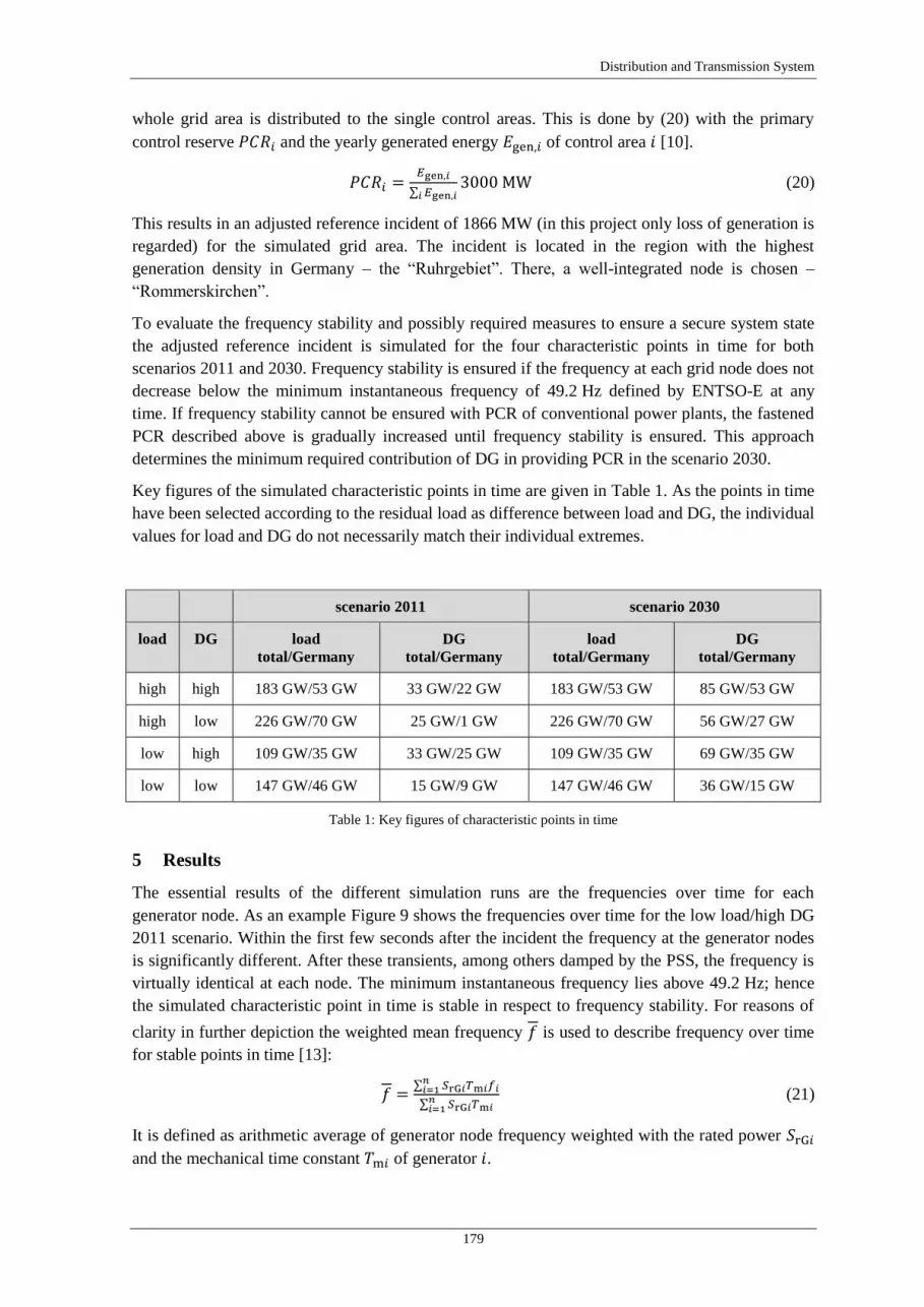
Distribution and Transmission System
179
whole grid area is distributed to the single control areas. This is done by (20) with the primary
control reserve 𝑃𝐶𝑅𝑖 and the yearly generated energy 𝐸gen,𝑖 of control area 𝑖 [10].
𝑃𝐶𝑅𝑖 =𝐸gen,𝑖
∑ 𝐸gen,𝑖𝑖3000 MW (20)
This results in an adjusted reference incident of 1866 MW (in this project only loss of generation is
regarded) for the simulated grid area. The incident is located in the region with the highest
generation density in Germany – the “Ruhrgebiet”. There, a well-integrated node is chosen –
“Rommerskirchen”.
To evaluate the frequency stability and possibly required measures to ensure a secure system state
the adjusted reference incident is simulated for the four characteristic points in time for both
scenarios 2011 and 2030. Frequency stability is ensured if the frequency at each grid node does not
decrease below the minimum instantaneous frequency of 49.2 Hz defined by ENTSO-E at any
time. If frequency stability cannot be ensured with PCR of conventional power plants, the fastened
PCR described above is gradually increased until frequency stability is ensured. This approach
determines the minimum required contribution of DG in providing PCR in the scenario 2030.
Key figures of the simulated characteristic points in time are given in Table 1. As the points in time
have been selected according to the residual load as difference between load and DG, the individual
values for load and DG do not necessarily match their individual extremes.
scenario 2011 scenario 2030
load DG load
total/Germany
DG
total/Germany
load
total/Germany
DG
total/Germany
high high 183 GW/53 GW 33 GW/22 GW 183 GW/53 GW 85 GW/53 GW
high low 226 GW/70 GW 25 GW/1 GW 226 GW/70 GW 56 GW/27 GW
low high 109 GW/35 GW 33 GW/25 GW 109 GW/35 GW 69 GW/35 GW
low low 147 GW/46 GW 15 GW/9 GW 147 GW/46 GW 36 GW/15 GW
Table 1: Key figures of characteristic points in time
5 Results
The essential results of the different simulation runs are the frequencies over time for each
generator node. As an example Figure 9 shows the frequencies over time for the low load/high DG
2011 scenario. Within the first few seconds after the incident the frequency at the generator nodes
is significantly different. After these transients, among others damped by the PSS, the frequency is
virtually identical at each node. The minimum instantaneous frequency lies above 49.2 Hz; hence
the simulated characteristic point in time is stable in respect to frequency stability. For reasons of
clarity in further depiction the weighted mean frequency 𝑓 is used to describe frequency over time
for stable points in time [13]:
𝑓 =∑ 𝑆rG𝑖𝑇m𝑖𝑓𝑖
𝑛𝑖=1
∑ 𝑆rG𝑖𝑇m𝑖𝑛𝑖=1
(21)
It is defined as arithmetic average of generator node frequency weighted with the rated power 𝑆rG𝑖
and the mechanical time constant 𝑇m𝑖 of generator 𝑖.

Smart Nord Final Report
180
Figure 9: Frequency over time at each generator node in low load/high DG 2011 scenario (incident after 1 s)
The results for all high load points in time (left side) and low load points in time (right side) with
respectively high and low DG are shown in Figure 10. The high load points in time are stable in
both scenarios 2011 and 2030 without additional fastened PCR provided by DG. Three out of four
low load points in time are also stable without further measures; the only exception is the low
load/high DG point in time in scenario 2030. In this point in time a provision of fastened PCR by
DG in the amount of 1.6 % of their actual power feed-in is required to stabilise the system (the
situation without provision of fastened PCR is not depicted for this point in time, because it is not
stable). In comparison to the simulation results for the other points in time it shows a different
behaviour. The decrease of the frequency is faster due to the reduced inertia, the increase likewise
because of the fastened PCR.
Figure 10: Mean frequency over time in high load (left) and low load (right) points in time (incident after 1 s)
This basic correlation between rate of frequency decrease and inertia is not obvious for the other
points in time, because it is overlaid by another effect. In the chosen modelling approach at high
DG points in time the voltage decrease at grid nodes after the incident is relatively greater that at
low DG points in time. This can be explained first with the constant power feed-in modelling of
DG. A reduction of voltage at a grid node immediately leads to a greater current. Due to the
subsequent greater current on the connecting transmission lines the voltage drops on this
0 10 20 30 40 5049.2
49.4
49.6
49.8
50
time (s)
freq
uen
cy (
Hz)
0 1 2 3 4 549.8
49.85
49.9
49.95
50
50.05
time (s)
freq
uen
cy (
Hz)
0 10 20 30 40 5049.2
49.4
49.6
49.8
50
50.2
time (s)
freq
uen
cy (
Hz)
high DG 2030
low DG 2030
high DG 2011
low DG 2011
0 10 20 30 40 5049.2
49.4
49.6
49.8
50
50.2
time (s)
freq
uen
cy (
Hz)
high DG 2030
low DG 2030
high DG 2011
low DG 2011
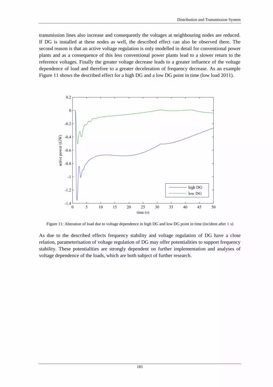
Distribution and Transmission System
181
transmission lines also increase and consequently the voltages at neighbouring nodes are reduced.
If DG is installed at these nodes as well, the described effect can also be observed there. The
second reason is that an active voltage regulation is only modelled in detail for conventional power
plants and as a consequence of this less conventional power plants lead to a slower return to the
reference voltages. Finally the greater voltage decrease leads to a greater influence of the voltage
dependence of load and therefore to a greater deceleration of frequency decrease. As an example
Figure 11 shows the described effect for a high DG and a low DG point in time (low load 2011).
Figure 11: Alteration of load due to voltage dependence in high DG and low DG point in time (incident after 1 s)
As due to the described effects frequency stability and voltage regulation of DG have a close
relation, parameterisation of voltage regulation of DG may offer potentialities to support frequency
stability. These potentialities are strongly dependent on further implementation and analyses of
voltage dependence of the loads, which are both subject of further research.
0 5 10 15 20 25 30 35 40 45 50-1.4
-1.2
-1
-0.8
-0.6
-0.4
-0.2
0
0.2
time (s)
activ
e po
wer
(G
W)
high DG
low DG

Smart Nord Final Report
182
6 Conclusion
Within the research project Smart Nord the work package 4.1 developed an overall system model.
This model is an extension of the integrated grid and power market model INES and comprises the
transmission system, underlying distribution grid sections at selected UHV nodes, the wholesale
electricity market as well as the primary control reserve market and enables integrated analyses of
stationary and dynamic processes. The two evaluation scenarios 2011 and 2030, which have been
defined by the interdisciplinary working group Scenario Design, were implemented into this
simulation environment. For this, the existing integrated grid and power market model INES was
extended by generation forecasts and grid expansions for the future outlook and several new
approaches as for instance a reactive power management. Beyond that, models required for the
frequency stability studies were added. Consequently, the stationary analyses as well as the
frequency stability studies can be carried out based on the same asset data and simulation models
and within one process from market simulation over stationary system states to stability studies that
uses the results from one step as start value for the next step.
The simulation environment has been originally developed to represent the year 2011. Grid and
market model were evaluated and optimised for the characteristics and the given public data for
this specific year. The integration of the future outlook scenario 2030 into the system model was a
major task within this research project. The current discussions about grid expansion and
possibilities of future grid operation show the uncertainties and challenges for the future energy
supply system. In order to gain valid stationary system states for the scenario 2030 within the
system model several new developments for the transmission system and market model were
needed, because stable and valid grid states were rarely given without further measures. The grid
model had to be extended far above the discussed grid expansion plans (because these plans only
look forward to the year 2020). The alternated power plant allocation and dimensioning (see Work
Group Scenario Design), and the changed power plant dispatch led to entirely new load flow
situations.
It was shown, that the future outlook 2030 within the simulation model leads to high loads of
power lines and a high demand of reactive power provision of the underlying voltage levels. At
many points in time the conventional power plants, which normally provided the reactive power
within the simulation model, were displaced by distributed generation units. Hence, the reactive
power provision had to be rearranged within the simulation model. The high voltage band
violations in the simulation model were minimised with reactive power management approaches
for the German transmission system model. These approaches were evaluated considering the DG
units in the distribution grid section to quantify the provision of DG in the underlying voltage
levels within the German transmission system model. For further analyses these approaches have to
be evaluated in the overall transmission system model and within more detailed distribution grid
sections, as e.g. in the transfer project “iQ-Regler”54
. With the new challenges of the future outlook
for the year 2030 within the simulation model, including the high load of power lines and the high
demand of reactive power, more advanced solutions are needed to improve the permissibility of
stationary system states, as e.g. optimal power flow solutions, which have not been part of the
research project Smart Nord.
To evaluate the frequency stability four characteristic points in time were identified and simulated
in detail: high load/high DG; high load/low DG; low load/high DG; low load/low DG. For all
characteristic points in time the same incident was assumed: the loss of generation of about
1866 MW. This incident corresponds to the primary control reserve reference incident for the grid
54
http://smartnord.de/downloads/Praesentationen_Abschlusstagung/iQ-Regler.pdf

Distribution and Transmission System
183
area Continental Europe defined by ENTSO-E though was adapted because of the different size of
the regarded grid area. Within the developed model the frequency stability could be ensured for the
reference scenario as well as the future scenario. Nevertheless, temporarily a contribution of DG in
frequency control was necessary. For this purpose wind generation had to provide fastened PCR
linearly within 5 s, solar generation within 1 s. The characteristic point in time, which required this
contribution, was low load/high DG in the scenario 2030 with a required amount of fastened PCR
at the high of 1.6 % of the current feed-in power of wind and solar generation.
The developed model does not consider active voltage control by DG after the incident. Therefore a
high share of DG in interaction with the voltage dependence of loads has a decelerating influence
on the frequency over time after an incident. The usability of this effect for active voltage control
design of DG and its actual height as well as the future development of voltage dependence of
loads are subject of current research. For this, the developed model will be extended by more
detailed models for aggregated DG as well as its active power and voltage control, the turbine
control of power plants, a secondary reserve market and the above mentioned optimal power flow
approach to gain control reference values.


Distribution and Transmission System
185
Work Package 4.2: Low-Voltage Grid Modelling and Grid
Compatibility Assessment
Stefanie Koch56
, Marco Zobel55
and Bernd Engel56
Abstract
It is possible to manage the supply of active power with small decentralized power generators within a
defined distribution grid. To get a feeling for the real and effective capability of decentralized power
suppliers, micro combined heat and power (CHP) systems have been evaluated. Variances and restrictions
that are specific to the system have been validated through simulation and lab tests. Such systems would
typically be used to supply single-family homes. The electrical power is between 0.2 and 1.5 kWel. To
compare different systems with another reference, load profiles as defined in VDI 4655 [23] were used.
Numerous scenarios have therefore been calculated using MATLAB-Simulink models as well as test devices.
All systems are restricted by the quantity of heat, that is, all heat must be used or buffered. Because of this
requirement, it is possible that the CHP system will be shut down in months with lower or no heat demand.
The BlueGEN system is an exception. Because of its technical characteristics, heat limitation is only
marginal with this kind of system, and it is thus ideal as a decentralized power generator. To achieve critical
or relevant influence, it is necessary to have high penetration of these systems within the distribution grid.
Furthermore, the Smart North scenarios in the form of holistic network models have been analysed. For this
purpose, several rural and an urban low-voltage (LV) networks were implemented in the grid calculation
software PowerFactory and linked to a medium-voltage (MV) benchmark-network. In a first step, these
networks have been equipped with consumer loads and supplemented by production units from other work
packages. With this model, a comprehensive analysis of the grid status in 2011 (reference) and 2030 was
possible. It can be concluded that the ongoing integration of decentralized generation units in distribution
grids will entail reasonable reinforcements of the networks.
1 Supply of Active Power Using Micro-CHP Systems
It is possible to use micro-CHP systems to meet the energy demand of single-family houses.
Typically, CHP systems cover the base load of power and heat. Additional heat requirements can
be covered using a peak heater in an efficient manner, while surplus of power is fed into the grid.
The required fuel can be taken continuously out of the natural gas grid. That allows a predictable as
well as specific active power supply. The variances and restrictions of micro-CHP systems are
evaluated and the service capacities of targeted active power supply are validated within the
following sections.
1.1 Pre-Evaluation of Micro-CHP Systems
Only commercial CHP systems for single-family houses were considered for pre-evaluation.
Despite this restriction, there is sufficiently high potential for installing high numbers of micro-
CHP systems within the supply grid. Examples of commercial CHP systems are shown in
Figure 12. With the exception of the BlueGEN system, which is based on a solid oxide fuel cell
generator, all other systems are generically referred to as power-generating heating systems. That
means that these systems will always generate heat that must be buffered or used. If no heat is
required, these systems must be shut down at a certain temperature limit.
55
EWE-Forschungszentrum für Energietechnologie e.V., 26129 Oldenburg, Germany,
[email protected], Bereich Brennstoffzellen / KWK-Systeme 56
Technische Universität Braunschweig, 38106 Braunschweig, Germany,
[email protected], elenia

Smart Nord Final Report
186
Stirling engine:
Dachs Stirling
SE [24]
Engine:
Vaillant ecopower
1.0 [25]
SOFC fuel cell:
HEXIS Galileo
1000N [26]
PEM fuel cell:
Viessmann
Vitovalor 300-P [27]
SOFC fuel cell:
CFCL
BlueGEN [28]
Figure 12: Commercial micro-CHP systems with different cogeneration technologies in the power range of up to 1.5 kWel
In order to identify suitable micro-CHP systems with a high potential for active power supply, the
heat or, rather, temperature dependence must be given particular consideration. To classify CHP
systems, the ratio between generated power and useful heat – the power to heat ratio – is used. The
higher this value, the lower the generated amount of heat. High power to heat ratios result in longer
operating times for a power supply, while low numbers result in shorter operating times that are
limited by an overcapacity of generated heat. Systems based on electrochemical energy
transformation, such as fuel cells, have higher efficiencies and power to heat ratios than
conventional combustion engines.
To compare and evaluate different systems, a representative scenario was defined using the
standard load profiles from the guideline VDI 4655 [23]. These include heat and power demand
sets for single-family houses and apartments with typical daily demands to a resolution of one
minute. For Germany, fifteen climate zones are defined with typical ambient temperature profiles
based on values from the Deutscher Wetterdienst (German Meteorological Service). As shown in
Table 2, a year is divided into seasons, such as winter, summer and transition, as well as working
days and Sundays. To cover heat transmission by solar radiation, there is also a subdivision for
cloudiness during the heating period. For every day type there exists a typical heat demand profile
with standardized energy factors for heating, hot water and power. The heat demand depends on
the year of construction of the building and the insulation level. The hot water and power demand
depends on the number of inhabitants and quantity of equipment. The distribution and frequency of
day type depends on the climate zone.
Season Weekday W Sunday S
Clear H Cloudy B Clear H Cloudy B
Transition Period Ü ÜWH ÜWB ÜSH ÜSB
Summer S SWX SSX
Winter W WWH WWB WSH WSB
Table 2: Standard reference days based on VDI 4655
For a single family house in Oldenburg (climate zone TRY03), these values result from annual base
demands for heat of 15,000 kWh/a, hot water of 2,000 kWh/a and power of 4,000 kWh/a, as can be
seen in Table 3.

Distribution and Transmission System
187
Reference
Days
SWX SSX ÜSH ÜWH ÜSB ÜWB WSH WWH WSB WWB ∑year
Days per
year
71 10 8 33 19 87 5 28 21 83 365
Power
[kWh/d]
8.8 9.7 12.2 9.9 13.3 10.9 12.6 10.9 14.2 11.9 4,000
Heat
[kWh/d]
0 0 37.2 25.8 33.8 36.1 85.3 75.6 63.8 74.5 15,000
Hot Water
[kWh/d]
3.8 6.6 7.9 4.4 8.3 4.9 11.4 6.0 8.6 5.6 2,000
Table 3: Overview of the energy demand of a single-family house (climate zone TRY03/Oldenburg) on different VDI
reference days
Figure 13: Power and heat load profiles for a single-family house on a VDI ÜWH-day and PEMFC-CHP profiles with
0.75 kWel and 1 kWth
By using those available load profiles, the achievable cover ratios and system characteristics can be
evaluated. Shown in Figure 13 are power and heat load profiles for a single-family house on a
ÜWH-day. The generator profile is given with electrical power of 0.75 kWel and thermal power of
1 kWth, representing a PEMFC-CHP system. In addition, the specific power demand for that day is
9.92 kWel, heat demand is 25.75 kWth and domestic hot water demand is 4.39 kWhth. The low
overnight heat demand causes the CHP system to start at 4:00 pm. If no heat is required, it is
possible to reduce electrical and thermal power by modulation. Lower numbers for active power
are expected for summer days. The minimum active power level would be 0.25 kWel. The technical
concept of the CHP system combined with the high electrical efficiency of 60 % at 1.5 kWel and
the low amount of heat of 0.6 kWth allows almost continuous operation of the BlueGEN system.
The laboratory evaluation therefore focussed on that system.

Smart Nord Final Report
188
1.2 Laboratory Validation of the CHP System
The required load profiles can be simulated using an autonomous test environment with integrated
control loops developed by NEXT ENERGY. The BlueGEN system has therefore been connected
electrically and hydraulically to this system. All input and output flows can be calculated exactly
from sensor readings. Day profiles have been combined in such a manner that a year can be
simulated in a time lapse test. Figure 14 shows the entire system consisting of the CHP unit, the
heat buffer and an additional peak burner (condensing boiler).
Figure 14: NEXT ENERGY test environment for CHP and heating systems
1.3 Determined Potentials of Micro-CHP Systems
The total amount of active power is defined by the difference between the electrical load demand
and the energy supplied by the CHP unit. To reduce the necessary measuring time and to get a
better understanding of the process, a model of the system was developed on a MATLAB-Simulink
basis and validated using characteristics that had already been measured. All real components or,
rather, sub-systems have been implemented, as have control procedures and the temperature
dependency of flow temperature.
Using the standardized load profiles, measured and simulated results can be compared in an easy
and transparent way. The characteristics and temperature levels within the thermal buffer store in
the simulation fit the measurements very well. An important quality requirement is thus fulfilled. In
Figure 15, the seasonally dependent heat demand (red) for different day types is shown. As
expected, the heat demand decreases to hot water demand only in summer time (red line). The
green line represents the daily power demand. Simulated and measured surplus power fed into the
grid also fit very well (dotted blue, blue line). In summary, the evaluated BlueGEN CHP system
matches the requirements for a controlled active power supply. Nevertheless, its high potential can
only be used if a high number of systems are installed in the local grid.

Distribution and Transmission System
189
Figure 15: Power feed to the grid according to seasonal heat demand
2 Assessment of the Integration of Decentralized Generators in the Distribution
Grid
The objective of this subsection is to determine whether the increasing penetration of decentralized
generating units has an adverse effect on the power quality.
2.1 Methodology
Two scenarios have been implemented to achieve the aforementioned objective. The first scenario
takes into account the situation prevailing in 2011, the latter scenario the situation expected to be
the case in 2030. For both scenarios a power grid model involving the medium- and low-voltage-
level has been developed. The power grid model is based on the Cigre-Benchmark Grid for the
medium-voltage level and has been augmented using 71 low-voltage-grids being based on real
grids existing in Germany. The power grid model is illustrated in Figure 16. In total, the model
comprises 12,000 loads representing single residential buildings. For the scenario 2011 and 2030,
700 and 2,750 decentralized generators, respectively, have been integrated.
Figure 16: Implemented power grid model
Figure 17: Grid reinforcement measures
Two key issues, being common when integrating decentralized units, are depicted in Figure 16. At
the medium-voltage-level it is likely that critical congestions occur at single feeders, bus bars, or
substations. Many transformer stations include an in-built overload capability. Consequently, they

Smart Nord Final Report
190
can cope with temporary overload periods, affecting merely their aging behaviour. In terms of
cables, predominantly underground cables are deployed in MV and LV power grids. The
permissible wiring ampacity must not be exceeded by any means. Critical situations can especially
occur during temporary reversals of the power flow.
The second key issue is the occurrence of critical overvoltages at the low-voltage-level. Small
photovoltaic modules are connected at the point of common coupling of residential buildings.
Particularly at the end of feeders the voltage can exceed the admissible range.
Several simulations were carried out with a view to observing differences in the individual
scenarios. As can be seen from Table 4, two calculations per scenario have been conducted, i.e.
high load condition and load flow reversal condition.
Scaling factor
Low-Voltage Medium-Voltage
High load Load flow
reversal High load
Load flow
reversal
Load 1 0.25 - -
Wind power - - 0 1
Solar power 0 0.85 0 0.85
CHP units 0 1 0 1
Table 4: Scaling factor of load and generating units for the high load and load flow reversal case
The results have been assessed taking the following requirements into account. The maximum
capacity utilization factor of MV-transformer substations and MV-cables is at 60 % for the high
load and at 100 % for the load flow reversal calculation. Distribution transformers and LV-cables
can be loaded up to 100 % in both cases. The maximum magnitude of the voltage change is ±10 %
of the nominal voltage. In addition, the maximum voltage rise at grid nodes, where generating units
are coupled, is 2 % and 3 % at the MS- and LV-level, respectively.
In case of an overvoltage at one of the nodes or a congestion of the network equipment, grid
reinforcement measures have been implemented for the ensuing calculations. As remedial actions
we take into account the following grid reinforcement measures. These measures are implemented
into the grid as depicted in Figure 17:
Optimization of disconnection points in cable distribution cabinets
Implementing a parallel cable
Separating the LV-grid and installing a second distribution transformer
Supplanting the distribution transformer with a new one with a higher rated power
2.2 Scenario 2011
The first scenario under investigation is the high-load scenario. The relevant input parameter can be
seen in Table 4. The findings reveal that all voltages occurring in the power grid are within the
permissible range (Figure 18). Moreover, the capacity utilization of all cables and transformer
stations are below the determined load limit. This result was to be expected as the high load
scenario is commonly used by grid operators to design and construct the grid.

Distribution and Transmission System
191
Figure 18: Grid reinforcement measures (High load scenario 2011)
The second case analysed is the load flow reversal scenario of 2011. As can be seen from
Figure 19, the average photovoltaic power installed in this grid is still below the average maximum
load per PCC in this case. However, as this is the case only in the low-voltage-grid, in the medium-
voltage-grid also wind power has been taken into account. The results of the simulations clearly
show that the voltages of virtually all nodes are within the permissible range. Still, a small fraction
(1 %) of all nodes exhibits voltages exceeding the limit of 1.1 p.u. Thus, a preliminary conclusion
might be that the design of power grids based solely on the high load scenarios is no longer
sufficient to resemble the real situation prevailing in power grids.
Figure 19: Characteristics of load flow reversal scenario 2011
For a more thorough investigation, Figure 20 illustrates the voltage increase both at LV-level and
MV-level. It is obvious that particularly at the MV-level the voltage of a significant amount of
nodes exceeds the 2 %-limit. At the LV-level the proportion of voltages exceeding the 3 % limit is
less but still at 11 %.
Figure 20: Calculation results (Load flow reversal scenario 2011)

Smart Nord Final Report
192
In the second calculation all cables and transformers have been within the limits of the determined
maximum capacity utilization factor. However, to mitigate the increase of the voltage at the nodes
we proposed and implemented several grid reinforcement measures (Figure 21). These measures
are commensurate to increase in voltage, thus the majority of the measures have been proposed for
the MV-level. At the MV-level 16 % of the grid length is subject to reinforcement. An additional
amount of three transformer stations have to be supplanted with more powerful ones.
Figure 21: Requirement for grid reinforcement measures (Load flow reversal scenario 2011)
2.3 Scenario 2030
The simulation data for the year 2030 was obtained by increasing the penetration of decentralized
generators (see Figure 22). In total the amount the installed power increased by the factor 2.7. As
the scenario of 2011 clearly revealed, the simulation for the load flow reversal is more suitable to
identify critical grid congestions. Consequently, in for the scenario 2030 we omitted the high load
scenario.
Figure 22: Installed generating capacity (Load flow reversal scenario 2030)
As can be seen from the two bar charts in Figure 23, the voltage at the majority of MV-nodes
exceeds the required limits. Only 23 % of the voltages are within the admissible range. At 10 % of
the nodes the voltage is 11 % higher than the nominal voltage which could entail adverse effects on
the power quality. In terms of the voltage increase at the connection points of generating units it
can be derived that only 23 % of the nodes meet the voltage requirements. The same conclusion
also applies for the condition in the LV-level of the power grid (Figure 24). The maximum
magnitude of the voltage change was calculated as an increase of 14 %. However, 76 % of the
nodes exhibit voltages within the admissible range, but a more detailed view reveals that especially
at nodes with attached generating units the voltage is significantly too high (Figure 24, right-hand
side).

Distribution and Transmission System
193
Figure 23: Calculation results in terms of voltage at MV-level (Load flow reversal scenario 2030)
Figure 24: Calculation results in terms of voltage at LV-level (Load flow reversal scenario 2030)
Based on the simulation results we applied the same pattern as in the scenario 2011 to identify
relevant grid reinforcement measures. Both results are compared in Figure 25. Whereas the
reinforcement requirement in the LV-level in terms of cables significantly increased, the amount
slightly decreased at the MV-level. In contrast, the situation regarding the necessary replacements
of transformers is striking. Particularly at the MV-level 58 % of the installed transformer capacity
has to be supplanted with more powerful ones. On the LV-level only a slight increase of 1 % was
found.
Figure 25: Total grid reinforcement requirement (Load flow reversal scenario 2030)
2.4 Conclusion
In conclusion, it can be noted that the ongoing installation of decentralized generators will entail a
tremendous grid reinforcement demand. In the present grid we increased the amount of
decentralized units by a factor of 2.7. This will lead to the requirement of reinforcing 32 % of all
cables and 58 % of all transformers at the MV-level. Similarly, at the LV-level 11 % of the cables
and 7 % of the transformers have to be supplanted until 2030.

Smart Nord Final Report
194
References
[1] T. Breithaupt, T. Rendel, C. Rathke, L. Hofmann, “Modeling the Reliability of Large Thermal Power
Plants in an Integrated Grid and Market Model,” 2012 IEEE International Conference on Power
System Technology (Powercon), Auckland, New Zealand, 2012.
[2] T. Rendel, C. Rathke, T. Breithaupt, L. Hofmann, “Integrated Grid and Power Market Simulation,”
IEEE PES General Meeting, San Diego, CA, USA, 2012.
[3] T. Rendel, C. Rathke, L. Hofmann, “Integrated Grid and Power Market Simulator,” in: ew - das
Magazin für die Energiewirtschaft, no. 20, pp. 20-23, 2012.
[4] T. Breithaupt, S. Garske, T. Rendel, L. Hofmann, “Methodological Approach for Integrated Grid and
Market Simulation of Coherent Distribution and Transmission Systems,” EnviroInfo 2013, Hamburg,
Germany, 02.-04. September 2013.
[5] F. Fuchs, R. Dietz, S. Garske, T. Breithaupt, A. Mertens, L. Hofmann, “Challenges of Grid Integration
of Distributed Generation in the Interdisciplinary Research Project Smart Nord,” IEEE 5th
International Symposium on Power Electronics for Distributed Generation Systems (PEDG), Galway,
Ireland, 24.-27. June 2014.
[6] K. Rudion, A. Orths, Z. A. Styczynski, K. Strunz, “Design of Benchmark of Medium Voltage
Distribution Network for Investigation of DG Integration,” IEEE Power Engineering Society General
Meeting.
[7] T. Leveringhaus, L. Hofmann, “Optimized voltage and reactive power adjustment in power grids
using the least-squares-method: Optimization of highly utilized power grids with stochastic renewable
energy-sources,” IEEE International Conference on Power and Energy Systems (ICPS), Chennai,
Indien, 22.12 – 24.12. 2011.
[8] C. Rathke, “Entwicklung eines Modells für die integrierte Simulation der europäischen
Übertragungsnetze und Strommärkte,” Aachen, Shaker Verlag, 2013.
[9] European Network of Transmission System Operators (2009). “Continental Europe Operation
Handbook – P 1: Load-Frequency Control and Performance,” Brussels, Belgium, 2009.
[10] European Network of Transmission System Operators. “Continental Europe Operation Handbook –
Appendix 1: Load-Frequency Control and Performance,” Brussels, Belgium, 2004.
[11] B. R. Oswald, “Berechnung von Drehstromnetzen,” vol. I. Wiesbaden: Vieweg+Teubner, 2009.
[12] K.-D. Weßnigk, “Kraftwerkselektrotechnik,” vol. I. Berlin: vde-verlag, 1993.
[13] P. Kundur, “Power System Stability and Control,” vol I. New York: McGraw-Hill, 1994.
[14] IEEE Task Force on Load Representation for Dynamic Performance, “Load representation for
dynamic performance analysis,” IEEE Transactions on Power Systems, Vol. 8, No. 2, pp.472-482,
May 1993.
[15] IEEE Recommended Practice for Excitation System Models for Power System Stability Studies, IEEE
Std. 421.5-2005, April 2006.
[16] T. Breithaupt, T. Rendel, L. Hofmann, “INES - Integrierte Netz- und Energiemarktsimulation,” 15.
Dresdener Kreis 2014, Fachtagung der TU-Dresden, der Universität Hannover, der Universität
Magdeburg und der Gesamthochschule Duisburg: Elektroenergieversorgung, Leipzig, Deutschland,
19.-20. März 2014.
[17] K. Knorr, B. Zimmermann, D. Kirchner, M. Speckmann, R. Spieckermann, M. Widdel,
M. Wunderlich, R. Mackensen, K. Rohrig, F. Steinke, P. Wolfrum, T. Leveringhaus, T. Lager,
L. Hofmann, D. Filzek, T. Göbel, B. Kusserow, L. Nicklaus, P. Ritter, “Kombikraftwerk 2 /
RegenerativKraftwerk 2050: Wege zu einer 100%-Versorgung mit erneuerbaren Energien -
Abschlussbericht,” Pilotprojekt unter Förderung des Bundesministeriums für Umwelt, Naturschutz
und Reaktorsicherheit, August 2014.
[18] CIGRE Technical Brochure, Modeling and Dynamic Behavior of Wind Generation as it Relates to
Power System Control and Dynamic Performance, prepared by CIGRE Working Group C4.601 on
Power System Security Assesment, August 2007.
[19] R. Hollinger, L. Engesser, T. Erge, “Frequenzhaltung als Serviceleistung dezentraler
Solarstromspeicher,” R. Hollinger, M. Llerena Engesser, L. M. Diazgranados, T. Erge, VDE-
Kongress 2014, Frankfurt am Main, Deutschland, 20.-21.10.2014.
[20] IEEE Technical Report PES-TR13, “Interconnected Power System Response to Generation
Governing: Present Practice and Outstanding Concerns”.
[21] “Ten Years Network Development Plan,” ENTSO-E, 2014.

Distribution and Transmission System
195
[22] “Netzentwicklungsplan Strom,” 50Hertz Transmission GmbH, Amprion GmbH, TenneT TSO GmbH,
TransnetBW GmbH, 2012.
[23] Reference load profiles of single-family and multi-family houses for the use of CHP systems,
Technical guideline VDI 4655, 2008-5.
[24] Micro-CHP system Senertec Dachs SE (stirling engine), 2015.
[25] Micro-CHP system Vaillant ecopower 1.0 (gas engine), 2015.
[26] Micro-CHP system HEXIS Galileo 1000N (Solid Oxide Fuel Cell), 2015.
[27] Micro-CHP system Viessmann Vitovalor 300-P (Polymere Electrolyte Membran Fuel Cell), 2015.
[28] Micro-CHP system CFCL BlueGEN (Solid Oxid Fuel Cell), 2015.


System Theory for Active Distribution Grids
197
Sub-Project Five:
System Theory for Active Distribution Grids


System Theory for Active Distribution Grids
199
Overview on Sub-Project Five:
System Theory for Active Distribution Grids
Hans-Peter Beck57
, Mehrnaz Anvari58
, Christian Bohn57
, Timo Dewenter58
, Alexander
Hartmann58
, Detlev Heinemann58
, Wiebke Heins57
, Gerald Lohmann58
, Joachim Peinke58
,
Florian Pöschke57
, Mohammad Reza Rahimi Tabar58
and Benjamin Werther57
1 Work Package 5.1
In this sub-project we focus on the system theory of distribution grids and MicroGrids. In work
package 5.1 MicroGrids in different settings are investigated. Parameters of a virtual synchronous
machine that mimics the behaviour of a synchronous machine are optimized with respect to a cost
functional. Simulations as well as experiments to validate the obtained time series have been done
to achieve a realistic result. A MicroGrid consisting of inverters, such a special machine and a load
is also numerically optimized. A distributed frequency control for a MicroGrid was applied and
parameters adjusted such that with the help of communication the original load sharing of the
machines in the grid could be restored via a secondary control. Different models like a simple
transport model on various random networks have been investigated to characterize very resilient
network topologies.
2 Work Package 5.2
Work package 5.2 deals with the short-term stochastic dynamics of wind and solar power in order
to assess their effects on the stability of distribution grids. By means of power spectrum analyses
and increment statistics, frequent high magnitude fluctuations (flickering) are documented in both
wind power and solar irradiance. To help mitigate the risk of MicroGrid instability in the future, a
time delayed feedback method is proposed that is capable of suppressing some of the most extreme
flickering events in aggregated decentralized power production from wind turbines and
photovoltaic systems.
3 Work Package 5.3
Work package 5.3 has two main focuses. Part one improves a given experimental setup to a
demonstration plant for MicroGrids. The purpose of this demonstration plant is to validate the
theoretical results of the work packages WP 5.1 and WP 5.2. Furthermore, this work package deals
with the detection of islanding situations in MicroGrids. Due to the on-going increase of distributed
energy generation in the distribution grid a safe and sufficient fast detection of the transition from
the grid-connected to the islanding mode of the MicroGrid has to be ensured. Several islanding
detection methods and there applicability are tested and validated in the demonstration plant.
57
Clausthal University of Technology 58
University of Oldenburg


System Theory for Active Distribution Grids
201
Work Package 5.1: System Theory for MicroGrids
Wiebke Heins59
, Timo Dewenter60
, Benjamin Werther59
, Alexander Hartmann60
,
Christian Bohn61
and Hans-Peter Beck62
1 Introduction
This work package focuses on the design and optimization of control strategies for MicroGrids, as
well as on the characterization of resilient network topologies. Section 2 introduces the models of a
MicroGrid and a so-called virtual synchronous machine which are used later for the parameter
optimization in sections 3 and 4. Section 5 describes the distributed frequency control of a
MicroGrid, where the virtual synchronous machines used in the grid are able to communicate with
each other. The characterization of resilient network topologies for different models is done in
section 6 of this chapter.
2 Model and Setup for MicroGrid Optimization
Objective of the optimization is to find a parameter setup for the virtual synchronous machine (see
below section “Principle and Model of the Virtual Synchronous Machine”) with a droop controller
for frequency (P(f)) and an integral controller for secondary frequency control. The VISMA is
acting as the grid-building component in a MicroGrid. The MicroGrid contains two decentralized
energy sources which are interfaced to the grid via inverters and equipped with droop frequency
(P(f)) and droop voltage control (Q(U)) [46]. A load is connected to the grid at the central point of
the radial topology.
Figure 1: MicroGrid in island mode containing two inverters, one VISMA and one load
59
Clausthal University of Technology, 38678 Clausthal-Zellerfeld, Germany,
[email protected], Institute of Electrical Information Technology 60
University of Oldenburg, 26111 Oldenburg, Germany,
[email protected], Institute for Physics
61 Clausthal University of Technology, 38678 Clausthal-Zellerfeld, Germany,
[email protected], Institute of Electrical Information Technology 62
Clausthal University of Technology, 38678 Clausthal-Zellerfeld, Germany,
[email protected], Institute of Electrical Power Engineering and Energy Systems

Smart Nord Final Report
202
2.1 Principle and Model of the Virtual Synchronous Machine (VISMA)
The VISMA concept aims to set up the static and dynamic performance of the electromechanical
synchronous machine to a three phase hysteresis controlled inverter. Figure 2 shows the basic
structure of the VISMA.
Figure 2: Functional scheme of the VISMA [4]
The complete VISMA functional chain contains three sub-processes, the real-time measurement of,
the process computer and the hysteresis controlled inverter. The grid voltage is measured to feed
the virtual synchronous machine algorithm, which calculated the resulting stator currents of the
mathematical model of a synchronous machine. These stator currents are used as reference current
signals to drive fast hysteresis controlled inverter.
Figure 3 shows the equivalent circuit diagram of a synchronous machine stator
Figure 3: Equivalent circuit diagram of a synchronous machine stator (only one phase is shown)
The differential equation of the stator circuit is given in equation
𝒔 =𝟏
𝐋𝒔∙ (−𝐑𝒔 ∙ 𝒊𝒔 − 𝒖 + 𝒆) (1)
The parameter 𝒊𝑠, 𝒖 and 𝒆 are state variables in the form 𝒙𝑇 = [𝑥1 𝑥2 𝑥3], where 𝒊𝑠 is the stator
current, 𝒖 embodies the grid voltage, and 𝒆 equates to the induced EMF (electromotive force) in
the stator windings.

System Theory for Active Distribution Grids
203
𝒆 = 𝐸𝑝 ∙ (
sin(𝜑)
sin(𝜑 − 120°)
sin(𝜑 + 120°)) (2)
With the voltage 𝒖 and the current 𝒊𝑠 the electrical power is calculated by equation
𝑃𝑒𝑙 = ∑(𝑢𝑖 ∙ 𝑖𝑠,𝑖)
3
𝑖=1
(3)
The interconnection between the virtual electrical and virtual mechanical part of the machine is
specified by the polar wheel angle 𝜑.
= 𝜔 (4)
=1
J(𝑀𝑚𝑒𝑐ℎ −
𝑃𝑒𝑙
𝜔− 𝑀𝐷) (5)
The damping torque 𝑀𝐷 is defined by equation
𝐷 =1
Td
(kd ∙ − 𝑀𝐷) (6)
The differential equations (1) and (4) - (6) descripted the in the process computer used
mathematical of synchronous machine.
2.2 Model and Setup for MicroGrid Optimization
Line resistances in the grid are chosen as 1.67 Ω, line inductances as 1.514 mH. The nominal
frequency is 50 Hz, nominal voltage is 230 V. This mimics a typical low voltage grid in
Germany [2]. The load is constantly consuming active power at a level of 1.5 kW until at a certain
point in time, when it increases in a step-like way to a level of 3 kW. Objective of the optimization
is to find a set of parameters for the VISMA that enables the MicroGrid to overcome this
disturbance in a stable and beneficial way.
The model used for simulation is a system of differential-algebraic equations. Assuming small
frequency variations in the grid, the active power 𝑃𝑖(𝑡) and reactive power 𝑄𝑖(𝑡) injected to or
drawn from the grid at node 𝑖 are approximated by algebraic grid equations (see e.g. [47])
𝑃𝑖(𝑼(𝑡), ∆𝜽(𝑡))
= 𝐺𝑖𝑖𝑈𝑖2(𝑡)
− ∑ 𝑈𝑖(𝑡)𝑈𝑘(𝑡)(𝐺𝑖𝑘 cos(∆𝜃𝑖(𝑡) − ∆𝜃𝑘(𝑡)) + 𝐵𝑖𝑘 sin(∆𝜃𝑖(𝑡) − ∆𝜃𝑘(𝑡)))
𝑘∈𝑁(𝑖)
,
𝑄𝑖(𝑼(𝑡), ∆𝜽(𝑡))
= −𝐵𝑖𝑖𝑈𝑖2(𝑡)
− ∑ 𝑈𝑖(𝑡)𝑈𝑘(𝑡)(𝐺𝑖𝑘 sin(∆𝜃𝑖(𝑡) − ∆𝜃𝑘(𝑡)) − 𝐵𝑖𝑘 cos(∆𝜃𝑖(𝑡) − ∆𝜃𝑘(𝑡)))
𝑘∈𝑁(𝑖)
.
Here, 𝑁(𝑖) means the indices of all nodes in the grid that are neighbours to node 𝑖 (excluding index
𝑖 itself), 𝐺𝑖𝑘 + j𝐵𝑖𝑘 denotes the admittance of the line between nodes 𝑖 and 𝑘, 𝑈𝑖(𝑡) resp. 𝑈𝑘(𝑡) are
the root mean square values of the voltages at nodes 𝑖 resp. 𝑘, and ∆𝜃𝑖(𝑡) resp. ∆𝜃𝑘(𝑡) denote the
phase difference between nodes 𝑖 resp. 𝑘 and a reference node. The values 𝐺𝑖𝑖 and 𝐵𝑖𝑖 are given as

Smart Nord Final Report
204
𝐺𝑖𝑖 = 𝐺𝑖𝑖 + ∑ 𝐺𝑖𝑘
𝑘∈𝑁(𝑖)
, 𝐵𝑖𝑖 = 𝑖𝑖 + ∑ 𝐵𝑖𝑘 ,
𝑘∈𝑁(𝑖)
where 𝐺𝑖𝑖 + j𝑖𝑖 is the shunt admittance at node 𝑖.
As reference node, the node is used where the VISMA is connected. Without loss of generality, this
node is labelled as node no. 1. The simplified differential equations describing the VISMA which
are used for the simulation are
∆𝜃1(𝑡) = 0, ∆1(𝑡) = 0,
𝐽1(𝑡) = −𝑘d
𝑇d 𝜔1(𝑡) −
𝑘d
𝑇d 𝑑(𝑡) +
1
𝜔1(𝑡)(
1
𝑘P,1(𝜔nom − 𝜔1(𝑡)) + 𝑃sec,1(𝑡) − 𝑃1(𝑼(𝑡), ∆𝜽(𝑡))),
𝑇d(𝑡) = − 𝜔1(𝑡) − 𝑑(𝑡),
𝑇11(𝑡) = −𝑈1(𝑡) + 𝑈1,nom + 𝐾U (𝑈1,nom − 𝑈1(𝑡)),
where 𝑈1,nom is the nominal voltage setpoint for the VISMA, 𝜔nom is the nominal angular
frequency setpoint, 𝜔1(𝑡) the virtual frequency of the VISMA, 𝑑(𝑡) a virtual damping term, and 𝑇1
and 𝐾U parameters of proportional voltage control. The parameters 𝐽, 𝑘d and 𝑇d are design
parameters for the dynamic behaviour of the VISMA. The secondary control 𝑃sec,1(𝑡) is realized as
a simple integral controller governed by
𝑃sec,1(𝑡) = 𝑥I(𝑡),
I(𝑡) = 𝐾I(𝜔nom − 𝜔1(𝑡)).
with nominal angular frequency setpoint 𝜔nom = 2 ∙ 50 ∙ π.
The inverters are approximated as third-order systems of the form
∆𝑖(𝑡) = 𝜔𝑖(𝑡) − 𝜔1(𝑡),
𝑇𝑖𝑖(𝑡) = − 𝜔𝑖(𝑡) + 𝜔nom + 𝑘P,𝑖 (𝑃nom,𝑖 − 𝑃𝑖(𝑼(𝑡), ∆𝜽(𝑡))),
𝑇i𝑖(𝑡) = −𝑈1(𝑡) + 𝑈𝑖,nom + 𝑘Q,𝑖 (𝑄nom,𝑖 − 𝑄𝑖(𝑼(𝑡), ∆𝜽(𝑡))).
The parameters 𝑘Q,𝑖 are the droops of the Q(U)-droop control used in the inverters. In both VISMA
and inverter equations, 𝑘P,𝑖 denotes the droop of P(f)-droop-control.
The load is modelled as time series of active power.
3 Optimization of the Dynamical Behaviour of a Virtual Synchronous Machine
We examine both numerical and experimental the response of a Virtual Synchronous Machine (see
section “Principle and Model of the Virtual Synchronous Machine”) to a perturbation caused by a
jump in the virtual torque of the machine. This jump triggers the VISMA to provide output power,
which is taken from an DC energy storage. In the DEQs of a VISMA (cf., Eqs. (1)-(6)) are two
parameters which can be chosen freely and both influence the damping behaviour: The damping
factor 𝑘d and the damping time constant 𝑇d. These parameters should be chosen such that the
temporal development of the output power of the VISMA follows an exponential, i.e. we look for
minima of the cost functional

System Theory for Active Distribution Grids
205
𝐸 = ∫ 𝜆(𝑡) ⋅𝑡0+𝑇
𝑡0
‖ − 𝑃Soll‖22 d𝑡 (7)
where 𝑡0 is the time of the step of the torque, 𝑇 the measurement time, (𝑡) the active power,
𝑃Soll(𝑡) the desired exponential behaviour and
(8)
a weighting parameter. We numerically solve the DEQs of a VISMA connected with a stiff grid for
different parameter settings (𝑘d,𝑇d) and search for minima of Eq.(7) with the Downhill-Simplex
algorithm [5]. Here, we show exemplarily a result for a minimum of the cost functional for a time
constant 𝜏 = 0.4 s which determines the steepness of 𝑃𝑆𝑜𝑙𝑙(𝑡) (see Figure 4(a)). More details can
be found in [9].
Figure 4: (a) Comparison of measured and simulated VISMA frequency for 𝝉 = 𝟎. 𝟒 s and a minimum of the cost
functional for the given parameter values [9]. (b) The same for the active power feed-in of the VISMA [5]. Shown are
measured, simulated, and desired output power. Inset: Region close to step in virtual torque at time 𝒕𝟎 ≈ 𝟑 𝐬
4 MicroGrid Optimization
The set-up of the MicroGrid is depicted in Figure 1 and the corresponding equations are described
in section “Model and setup for MicroGrid optimization”. Like in the parameter optimization of the
VISMA (see section “Principle and Model of the Virtual Synchronous Machine”) we are looking
for minima of a cost functional defined by
(9)
where 𝑡𝑅 is the maximum of the relaxation times of frequency and voltage of all nodes after the
step-like increase at time 𝑡0 of the power demand of the load, the sum runs over the VISMA and
the two inverters (nodes 2 and 3), 𝑃Soll,𝑖(𝑡) is the desired active power output of the corresponding
node, and the weighting parameter is

Smart Nord Final Report
206
(10)
The parameters 𝛼 and 𝛽 determine the focus of the optimization, e.g., choosing a large 𝛼 results in
focusing on minimizing the area between output and desired power. In addition to this cost
functional we use constraints for the parameters to ensure that we get a realistic result. Therefore,
we apply bounds on parameters to ensure that the secondary control is slower than the VISMA
itself, and that the VISMA is not faster than a regular inverter corresponding to a bounded energy
feed-in.
We search for minima of Eq. (9) with the Downhill-Simplex algorithm [5]. Figure 5 shows two
results for different values of 𝛼 and 𝛽.
Figure 5: (a) Frequencies of the VISMA and the two inverters for a minimum of the cost functional for parameters
𝜶 = 𝟐. 𝟓 ⋅ 𝟏𝟎−𝟕, 𝜷 = 𝟏, 𝑱 = 𝟎. 𝟖𝟐𝟕, 𝒌𝐝 = 𝟏. 𝟗𝟒 ⋅ 𝟏𝟎−𝟑, 𝑻𝐝 = 𝟗. 𝟑𝟐 ⋅ 𝟏𝟎−𝟕, 𝑲𝐈 = 𝟐. 𝟕𝟐 ⋅ 𝟏𝟎𝟒, and 𝑲𝐏 = 𝟎.
Step in the load at time 𝒕𝟎 = 𝟏𝟎 𝐬. Inset: The same for the voltages of the four nodes. (b) The same for parameters
𝜶 = 𝟓 ⋅ 𝟏𝟎−𝟕, 𝜷 = 𝟎. 𝟎𝟏, 𝑱 = 𝟓. 𝟏𝟐 ⋅ 𝟏𝟎−𝟑 , 𝒌𝐝 = 𝟓𝟎. 𝟖𝟑, 𝑻𝐝 = 𝟎. 𝟕𝟖 ,𝑲𝐈 = 𝟐. 𝟎𝟕 ⋅ 𝟏𝟎𝟑, and 𝑲𝐏 = 𝟎. Inset:
Behavior of the voltages for the same scenario
4.1 Outlook
In addition, one could use “Parallel Tempering” [6] for searching minima [7] of the cost functional.
In this statistical physics method simple Monte Carlo simulations at different temperatures are
performed simultaneously while allowing for swaps of systems belonging to “neighbouring”
temperatures. With this procedure it is possible to overcome high barriers in the energy landscape
defined by the cost functional and therefore it is very likely to find a global optimum as possibly
the whole parameter space can be sampled.
5 Distributed Frequency Control for VISMA-Based MicroGrids
5.1 Objectives and Example Setup
A concept for distributed frequency control for MicroGrids is presented that is based on the virtual-
synchronous machine (VISMA). The control has to be robust against disturbances, communication
failures and sudden islanding. The key concept applied here is based on the “distributed-averaging
proportional-integral” (DAPI) controller presented in [8].

System Theory for Active Distribution Grids
207
A simulation example is presented here that illustrates the performance of the distributed control
strategy. A MicroGrid with three VISMA-controlled inverters of equal power rating, four loads and
a power source (for example a photovoltaic source without storage) is considered. Loads and power
source are not controlled, but act within known bounds. In grid-connected mode, the three VISMA-
controlled inverters are acting as grid-supporting units by supplying active power according to a
P(f) droop. When an islanding event occurs, they are able to perform primary control tasks, i.e. to
manage the transient and afterwards act as grid-building components, providing a constant voltage
and a common frequency. The level of the frequency is defined by the P(f) droops, as well as is
load sharing among the three VISMAs, e.g. by choosing the droops according to the power rating
of each VISMA.
Figure 6: MicroGrid with three VISMA-controlled inverters, four loads and one power source (e.g. a PV source without
storage). For distributed secondary control, the three VISMAs are able to communicate among each other as
indicated by the grey dotted line
After islanding, the grid frequency is usually not equal to the desired nominal frequency.
Therefore, a secondary frequency control is used to restore the nominal frequency.
5.2 Model Used for Design and Simulation
The model used for design and simulation is a system of differential-algebraic equations. Assuming
small frequency variations in the grid, the active power 𝑃𝑖(𝑡) and reactive power 𝑄𝑖(𝑡) injected to
or drawn from the grid at node 𝑖 are approximated by algebraic grid equations (see e.g.[47])
𝑃𝑖(𝑼(𝑡), ∆𝜽(𝑡))
= 𝐺𝑖𝑖𝑈𝑖2(𝑡)
− ∑ 𝑈𝑖(𝑡)𝑈𝑘(𝑡)(𝐺𝑖𝑘 cos(∆𝜃𝑖(𝑡) − ∆𝜃𝑘(𝑡)) + 𝐵𝑖𝑘 sin(∆𝜃𝑖(𝑡) − ∆𝜃𝑘(𝑡)))
𝑘∈𝑁(𝑖)
,
𝑄𝑖(𝑼(𝑡), ∆𝜽(𝑡))
= −𝐵𝑖𝑖𝑈𝑖2(𝑡)
− ∑ 𝑈𝑖(𝑡)𝑈𝑘(𝑡)(𝐺𝑖𝑘 sin(∆𝜃𝑖(𝑡) − ∆𝜃𝑘(𝑡)) − 𝐵𝑖𝑘 cos(∆𝜃𝑖(𝑡) − ∆𝜃𝑘(𝑡)))
𝑘∈𝑁(𝑖)
.
Here, 𝑁(𝑖) means the indices of all nodes in the grid that are neighbors to node 𝑖 (excluding index 𝑖
itself), 𝐺𝑖𝑘 + j𝐵𝑖𝑘 denotes the admittance of the line between nodes 𝑖 and 𝑘, 𝑈𝑖(𝑡) resp. 𝑈𝑘(𝑡) are
the root mean square values of the voltages at nodes 𝑖 resp. 𝑘, and ∆𝜃𝑖(𝑡) resp. ∆𝜃𝑘(𝑡) denote the
phase difference between nodes 𝑖 resp. 𝑘 and a reference node. The values 𝐺𝑖𝑖 and 𝐵𝑖𝑖 are given as
𝐺𝑖𝑖 = 𝐺𝑖𝑖 + ∑ 𝐺𝑖𝑘
𝑘∈𝑁(𝑖)
, 𝐵𝑖𝑖 = 𝑖𝑖 + ∑ 𝐵𝑖𝑘 ,
𝑘∈𝑁(𝑖)

Smart Nord Final Report
208
where 𝐺𝑖𝑖 + j𝑖𝑖 is the shunt admittance at node 𝑖.
The differential equations describing the VISMA
∆𝑖(𝑡) = 𝜔𝑖(𝑡),
𝐽𝑖(𝑡) = −𝑘d
𝑇d 𝜔𝑖(𝑡) −
𝑘d
𝑇d 𝑑𝑖(𝑡) +
1
𝜔𝑖(𝑡)(
1
𝑘P,𝑖(𝜔nom − 𝜔𝑖(𝑡)) + 𝑃sec,𝑖(𝑡) − 𝑃𝑖(𝑼(𝑡), ∆𝜽(𝑡))),
𝑇d,𝑖𝑖(𝑡) = − 𝜔𝑖(𝑡) − 𝑑𝑖(𝑡),
where 𝑈𝑖,nom is the nominal voltage setpoint for the VISMA, 𝜔nom is the nominal angular
frequency setpoint, 𝜔1(𝑡) the virtual frequency of the VISMA, 𝑑(𝑡) a virtual damping term. The
parameters 𝐽, 𝑘d and 𝑇d are design parameters for the dynamic behaviour of the VISMA. The
secondary control 𝑃sec,1(𝑡) is realized in different ways as described below.
The loads and power sources are modelled as timeseries of active and reactive power. They are
realized by algebraic constraints at the grid nodes.
5.3 Simulation Results for Secondary Frequency Control Strategies
Often, secondary frequency control is done by individual simple PI-controllers that are slow in
comparison to the primary droop control [8]. This means that in the VISMA equations the value
𝑃sec,𝑖(𝑡) for secondary control is governed by
𝑃sec,𝑖(𝑡) = 𝑥I,𝑖(𝑡),
I,𝑖(𝑡) = 𝑘I,𝑖(𝜔nom − 𝜔𝑖(𝑡)), 𝑖 = 1,2,3,
where 𝑥I,𝑖(𝑡) is an auxiliary state, and 𝑘I,𝑖 is the integral control constant. However, this does not
generally maintain the original load sharing. Especially in MicroGrids with storage units of limited
capacity, this can lead to undesirable behaviour. Figure 7 illustrates this effect: A disturbance
causes the secondary control to start not at the same time, but one after the other in timesteps of 0.1
second. Although all VISMAs have the same power rating, the control does not manage to restore
the power sharing. Nonetheless, the frequency is restored quickly. This effect cannot be overcome
by a completely decentralized control strategy.
Figure 7: Simulation result for decentralized PI-control: Injected active power (left) and VISMA frequencies (right)
The distributed control requires a communication link between all components that take part in
secondary control (Figure 7). The control law then reads in this example (see [8])
𝑃sec,𝑖(𝑡) = 𝑥I,𝑖(𝑡),
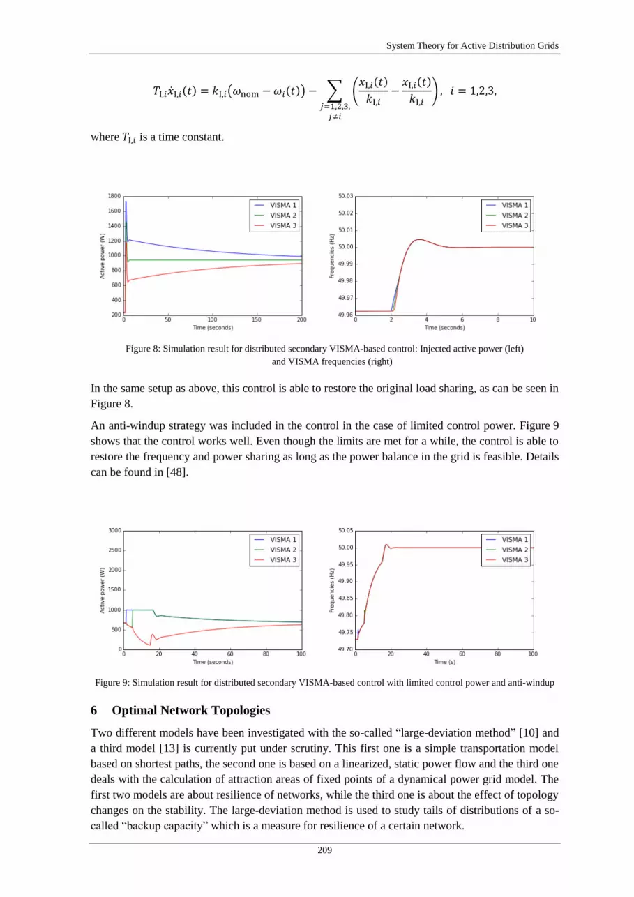
System Theory for Active Distribution Grids
209
𝑇I,𝑖I,𝑖(𝑡) = 𝑘I,𝑖(𝜔nom − 𝜔𝑖(𝑡)) − ∑ (𝑥I,𝑖(𝑡)
𝑘I,𝑖−
𝑥I,𝑖(𝑡)
𝑘I,𝑖)
𝑗=1,2,3,𝑗≠𝑖
, 𝑖 = 1,2,3,
where 𝑇I,𝑖 is a time constant.
Figure 8: Simulation result for distributed secondary VISMA-based control: Injected active power (left)
and VISMA frequencies (right)
In the same setup as above, this control is able to restore the original load sharing, as can be seen in
Figure 8.
An anti-windup strategy was included in the control in the case of limited control power. Figure 9
shows that the control works well. Even though the limits are met for a while, the control is able to
restore the frequency and power sharing as long as the power balance in the grid is feasible. Details
can be found in [48].
Figure 9: Simulation result for distributed secondary VISMA-based control with limited control power and anti-windup
6 Optimal Network Topologies
Two different models have been investigated with the so-called “large-deviation method” [10] and
a third model [13] is currently put under scrutiny. This first one is a simple transportation model
based on shortest paths, the second one is based on a linearized, static power flow and the third one
deals with the calculation of attraction areas of fixed points of a dynamical power grid model. The
first two models are about resilience of networks, while the third one is about the effect of topology
changes on the stability. The large-deviation method is used to study tails of distributions of a so-
called “backup capacity” which is a measure for resilience of a certain network.

Smart Nord Final Report
210
6.1 Transport Model
Distributions of the resilience of transport networks are studied numerically, in particular the large-
deviation tails. Thus, not only typical quantities like average or variance but the distributions over
the (almost) full support can be studied. For a proof of principle, a simple transport model based on
the edge-betweenness and three abstract yet widely studied random network ensembles are
considered here: Erdős-Rényi random networks (ER) with finite connectivity, small world
networks (SW) and spatial networks embedded in a two-dimensional plane. Using specific
numerical large-deviation techniques, probability densities as small as 10−80 are obtained here.
This allows to study typical but also the most and the least resilient networks. The resulting
distributions full the mathematical large-deviation principle, i.e., can be well described by rate
functions in the thermodynamic limit. The analysis of the limiting rate function reveals that the
resilience follows an exponential distribution almost everywhere. An analysis of the structure of the
network shows that the most-resilient networks can be obtained, as a rule of thumb, by minimizing
the diameter of a network (see Figure 10(b). Note that a small backup capacity corresponds to the
most resilient networks). Also, trivially, by including more links a network can typically be made
more resilient (see Figure 10(a)). On the other hand, the least-resilient networks are very rare and
characterized by one (or few) small core(s) to which all other nodes are connected. In total, the
spatial network ensemble turns out to be most suitable for obtaining and studying resilience of real
mostly finite-dimensional networks. Studying this ensemble in combination with the presented
large-deviation approach for more realistic, in particular dynamic transport networks appears to be
very promising. A more detailed description and more results can be found in [11].
Figure 10: (a) The average resilience 𝒄𝒃 as a function of the number 𝒏𝒆 of links for ER and spatial networks of size
𝑵 = 𝟒𝟎𝟎 [11]. (b) The average diameter 𝒅 as a function of the resilience 𝒄𝒃 for SW, ER and spatial networks of size
𝑵 = 𝟒𝟎𝟎, in the range of small value of 𝒄𝒃. The inset shows a scatter plot of the data for the entire range of backup
capacities for the SW case [11]
6.2 Power Flow Model
Distributions of the resilience of a power flow model against transmission line failures are studied
via a so-called backup capacity. In this linearized DC power flow model only active power is
investigated, where nodes in the network can either produce or consume active power. This power
is transported via lossless lines (edges in the graph) between the nodes, where the amount depends
on the phase angle difference between the two neighbouring nodes. We consider three ensembles
of random networks, and in addition, the topology of the British transmission power grid. The three

System Theory for Active Distribution Grids
211
ensembles are Erdős-Rényi random graphs, Erdős-Rényi random graphs with a fixed number of
links, and spatial networks where the nodes are embedded in a two-dimensional plane. We
numerically investigate the probability density functions (pdfs) down to the tails to gain insight into
very resilient and very vulnerable networks. This is achieved via large-deviation techniques, which
allow us to study very rare values that occur with probability densities below 10−160. We find that
the right tail of the pdfs towards larger backup capacities follows an exponential with a strong
curvature. This is confirmed by the rate function, which approaches a limiting curve for increasing
network sizes. Very resilient networks are basically characterized by a small diameter and a large
power sign ratio (c.f., Figure 11). The diameter of a network is the longest of all shortest paths in
the graph. The so-called “power sign ratio” is the fraction of edges that directly connect a producer
with a consumer of power. In addition, networks can be made typically more resilient by adding
more links. More details can be found in [12].
Figure 11: Average diameter 𝒅 (a) and power sign ratio 𝒑− (b) as functions of the backup capacity 𝑷𝑩 for all studied
network ensembles with size 𝑵 = 𝟒𝟎𝟎. Note that because of the gap in the data for ER and spatial networks, some
intermediate values of 𝑷𝑩 are not present [12]. Inset in (a) enlarges region for small 𝑷𝑩
6.3 Outlook
Numerical studies of the distribution of “maximum-disturbance” stability of power grids could also
be investigated [13]. The model is based on networks of oscillators. Here, we consider different
ensembles of random networks, like standard Erdös-Renyi and two dimensional spacial networks.
To access the distribution down to very small probabilities, we use specific large deviation
techniques [10]. The stability is given by a conservative estimation of an asymptotic stability
boundary, which is well known in stability theory. The starting point is the matrix A defined by
𝐉T ⋅ 𝐀 + 𝐀 ⋅ 𝐉 = 𝐄, 𝐉 being the Jacobean Matrix. By calculating the maximum disturbance of 𝐱,
which results in the quadratic form 𝑉 = 𝐱T ⋅ 𝐀 ⋅ 𝐱 = 𝜖(𝐱) not being a Lyapunov-function [14] of
the system any longer, the boundaries for the stability can be found. For comparison, for the given
networks also simple stability measures based on shortest paths [11], on the eigenvalues of the
Jacobi matrix and on a linearized power-flow model [12] are obtained.


System Theory for Active Distribution Grids
213
Work Package 5.2: System Theory of Generation and Loads
Gerald Lohmann63
, Mohammad Reza Rahimi Tabar63
, Mehrnaz Anvari63
, Detlev Heinemann63
and Joachim Peinke64
1 Introduction
With the decided exit from nuclear and fossil-fuel energy, and shares of wind and solar energy on
the rise, German power grids face increasing challenges regarding the integration and management
of said renewable sources [15]. Amongst others, issues of decentralized grid topology and the
maintenance of voltage and frequency stability is expected to become more and more difficult in
distribution grids with a high share of wind and solar power. Both renewable resources vary
considerably on virtually all time scales, with seasonal variations being in the order of months,
while weather-induced variations range from days to hours to minutes, and even seconds. Changes
in the magnitude of wind speed or solar irradiance are almost immediately translated into variations
in the output power of wind energy converters and photovoltaic (PV) systems [16].
Especially on very short time scales, these variations are stochastic in nature and thus difficult or
nearly impossible to predict. If more and more distributed generation from renewables is simply
integrated in existing power grids, thereby replacing conventional technologies such as hydro, gas,
coal, and nuclear power plants, system instabilities will be likely to occur [22]. Instead, to handle
this kind of volatile power production from decentralized renewables, and in order to contribute to
resilient power grids, a revision of traditional power grids becomes necessary [23], [24]. In
particular,
a reduction of correlation of variations may be aimed for by increased spatial dispersion and
diversification of sources (e.g. mix of solar and wind power),
flexible generators may be held available as back-up production capacity, which can be ramped
up and down quickly for balancing the load and generated power,
energy storage may be progressively introduced to the grid (although the cost of advanced
storage technologies, such as batteries, is often considered their main limitation),
trade and transfer of electricity across long distances may be increased, and finally
flexibility and grid management (including smart grid technologies) may be enhanced.
In the context of the last point, positive ramps caused by a sudden increase in renewable production
can, in principal, be limited very quickly at any time using power electronics. For negative
increments (ramp down), expensive energy storage systems are needed to help smooth out sudden
power decreases [17], [18], [19].
However, simply using electronics technology is not enough. It’s rather the interplay with the
intrinsic dynamics of the various interconnected conventional and renewable power systems that
determines the feasibility and effectiveness of any measure. For the best grid integration of wind
and solar energies, the physics of the wind and solar power fluctuations and their stochastic
behaviours must thus be understood in details. It’s mainly this aspect that the analyses presented in
63
University of Oldenburg, 26111 Oldenburg, Germany,
[email protected], Institute of Physics and ForWind 64
University of Oldenburg, 26111 Oldenburg, Germany,
[email protected], Institute of Physics and ForWind

Smart Nord Final Report
214
this report aim to contribute to, by documenting certain key characteristics of local high frequency
fluctuations in wind and solar power production.
As any power grid may be viewed as a complex system of systems, in which each sub-system is
comprised of a diverse set of passive and active components, the increasing share of intermittent
renewable energy links this complex network of power grids with the equally complex weather
system. Understanding the constituents of interaction of two complex systems, in this case power
grids and weather, and simulating their collective presence form the necessary basis from which an
efficient design of resilient power grids can emerge.
2 Material and Methods
The present work is based on relatively high frequency measurements from operating wind turbines
and continuous solar irradiance observations. Time series of wind speed, wind power, and global
horizontal irradiance (GHI) have been collected from several regions around the world (the United
States, Germany, Algeria, and Spain) with sampling rates ranging from 1 min-1
to 1 Hz. General
information on all datasets is presented in Table 1.
Dataset Variables Frequency Number of
observations
Wind farm, Germany (12 turbines with a
total of ~ 25 MW rated power)
Wind speed [ms-1
],
wind power [W]
1 Hz 15.3 * 106
Solar campaign, Germany GHI [Wm-2
] 1 Hz 12 * 106
Solar campaign, Hawaii, USA GHI [Wm-2
] 1 Hz 14 * 106
BSRN, Algeria GHI [Wm-2
] 1/60 Hz 3.7 * 106
BSRN, Spain GHI [Wm-2
] 1/60 Hz 1.3 * 106
Table 1: Details of available data
In order to facilitate comparisons between datasets, the wind power time series 𝑃(𝑡) are normalized
to the rated power 𝑃𝑟 of their respective turbines, hence scaled power
𝑃𝑠(𝑡) =𝑃(𝑡)
𝑃𝑟 (11)
is used. Similarly, and also to eliminate deterministic trends of diurnal and seasonal variations, all
𝐺𝐻𝐼(𝑡) time series are related to their respective theoretical clear-sky values 𝐺𝐻𝐼𝑐𝑙𝑒𝑎𝑟(𝑡). The
resulting time series of clear-sky index
𝑘∗ =𝐺𝐻𝐼
𝐺𝐻𝐼𝑐𝑙𝑒𝑎𝑟 (12)
is thus dimensionless. Figure 12 shows an example of single-point measurements of GHI for a
typical summer day with variable cloud cover in Northern Germany, measured with 1 Hz temporal
resolution, along with the corresponding 𝑘∗ time series.
As for obtaining the theoretical clear-sky irradiance, the clear-sky model presented in [20] is used
to derive time series of clear-sky irradiance for all available datasets. To ensure conservative results
when calculating 𝑘∗, only those times with solar elevation angles > 10° are considered for
processing. At lower angles (after sunrise; before sunset), the relatively low values of GHI, in
conjunction with path prolongation and the problem of small denominators, can result in unrealistic

System Theory for Active Distribution Grids
215
clear-sky index values [21]. Moreover, shadows from the surroundings frequently distort irradiance
measurements at times of low solar elevation angles.
Figure 12: Single-point measurements of global horizontal irradiance (GHI) for a typical summer day in Northern
Germany measured with 1 Hz temporal resolution (light blue). By means of the theoretical irradiance at clear sky
conditions (gray), deterministic patterns, such as diurnal variations may be removed effectively. The resulting clear-
sky index reduces variability to its atmospheric origin, without accounting for influences due to the time of day, or
the time of year. Note that measured irradiance frequently exceeds its theoretical clear-sky counterpart during times
of high variability, because solar irradiance is reflected by proximate clouds.
The first approach to describe the high-frequency characteristics of the aforementioned normalized
wind and solar time series is to analyse the power spectrum of wind turbine output power and solar
irradiance. By comparing the behaviour of a spectrum 𝑆(𝑓) with the well-known Kolmogorov-law
of turbulence, i.e. 𝑆(𝑓)~𝑓−5 3⁄ , conclusions regarding the nature of variations may be inferred.
Turbulent time series typically exhibit stochastic fluctuations at various time scales.
As these kinds of variations are of special interest to various stakeholders involved with
decentralized renewable power production, e.g. distribution system operators, a key aspect of this
work package is to further quantify and compare short-term fluctuations in wind and solar power
for different time intervals. In this context, the intermittency of a time series 𝑋(𝑡) can be described
by means of probability density functions (pdf) of the time series’ increments
Δ𝑋(𝑡, 𝜏) = 𝑋(𝑡 + 𝜏) − 𝑋(𝑡) (13)
for different time lags 𝜏.
Furthermore, a time-delayed feedback method is proposed for suppressing the short-term
intermittency of wind and solar power of multiple renewable generators. When considering such a
time dependent, spatially aggregated, cumulative power
𝑃∗(𝑡) = 𝑁−1 ∑ 𝑃𝑖(𝑡)𝑁𝑖=1 , (14)
based on N intermittent power systems, each of which supplies an output power 𝑃𝑖(𝑡), the time-
delayed feedback method proposes to save a fraction α of each generator’s power at time t. After Τ
seconds, this power is then fed into the grid in a delayed fashion, while only a fraction of (1 − 𝛼)
of the original power had been input to the grid at time t.
Thus, the new time delayed feedback power feed-in of each system is
𝑃𝑖(𝑡)𝑛𝑒𝑤 = (1 − 𝛼)𝑃𝑖(𝑡) + 𝜖𝑃∗(𝑡 − 𝑇), (15)
where, in general, 𝜖 ≤ 𝛼. The cumulative power output ∑ 𝑃𝑖(𝑡)𝑛𝑒𝑤𝑁
𝑖=1 depends on the delay lag Τ
and amplification α, and the method enables the assessment of operation strategies for power

Smart Nord Final Report
216
systems. It can be a complementary method for energy storage, on the existence of which it
obviously depends, and ramp-rate control. The effectiveness of this approach could even be
increased by using multiple energy storage systems, each with a different time lag T.
3 Results
Since the power spectrum of a time series reveals the contributions of different time scales to the
variations in the signal, the spectral analysis of wind velocity, scaled wind turbine power output,
and GHI in Figure 13 allows drawing conclusions on the nature of their respective variability. In
general, both wind turbines and photovoltaic cells convert wind velocity and solar irradiance
fluctuations into power fluctuations quickly. In case of wind power, the conversion dynamics take
place at short time scales in the order of seconds, while photovoltaic power conversion happens
almost instantaneously.
Both wind speed and wind power output of a single turbine have similar spectral behaviour at low
frequencies 𝑓 < 0.1 Hz, and both adhere to the Kolmogorov-law of turbulence, i.e.
𝑆(𝑓)~𝑓−5 3⁄ [23]. While the spectrum of wind speed fluctuations does not significantly differ from
the Kolmogorov-spectrum at higher frequencies, the spectrum of wind turbine power fluctuations
does, as is shown in Figure 12a. This is due to the finiteness of the reaction time scale of wind
turbines: the fast wind fluctuations are partly filtered, and slower wind fluctuations are
adiabatically converted into power output fluctuations. For cumulative power fluctuations of a
wind park, the filtering in the high frequency domain (𝑓 > 0.1 Hz) is even more emphasized, by
the way. Hence, the power output of an entire wind park has even weaker high frequency
fluctuations than that of a single turbine (not shown here).
In contrast to wind turbines, there is no considerable instrumental filtering in the conversion of
irradiance to power at 1 Hz sampling, and the turbulence-type spectrum of the Kolmogorov-law is
present in irradiance fluctuations of a single sensor for frequencies 0.001 < 𝑓 < 0.05 Hz (more
than one order of magnitude). This is shown in Figure 12b. The spectrum of the spatial average of
17 sensors shows some filtering in the higher frequency region, but already starting around 0.005
Hz, the reason of which is similar to the spectrum of total wind farm power that has been
mentioned above. Spatial aggregation thus dampens high frequency fluctuations in wind and solar
power to some degree.
Figure 13: Power spectra of (a) wind velocity (red) and wind power output of a single turbine (black) from high
frequency measurements in a wind park, and (b) irradiance fluctuations from high frequency measurements in Hawaii
for a single sensor (red) and the mean of 17 sensors (black) in log-log scale. The Kolmogorov-spectrum with an
exponent of 5/3 is represented by dashed lines in each plot. The insets of (a) and (b) show log-log plots of the
compensated energy spectra 𝑓5 3⁄ 𝑆(𝑓) as a function of frequency 𝑓.
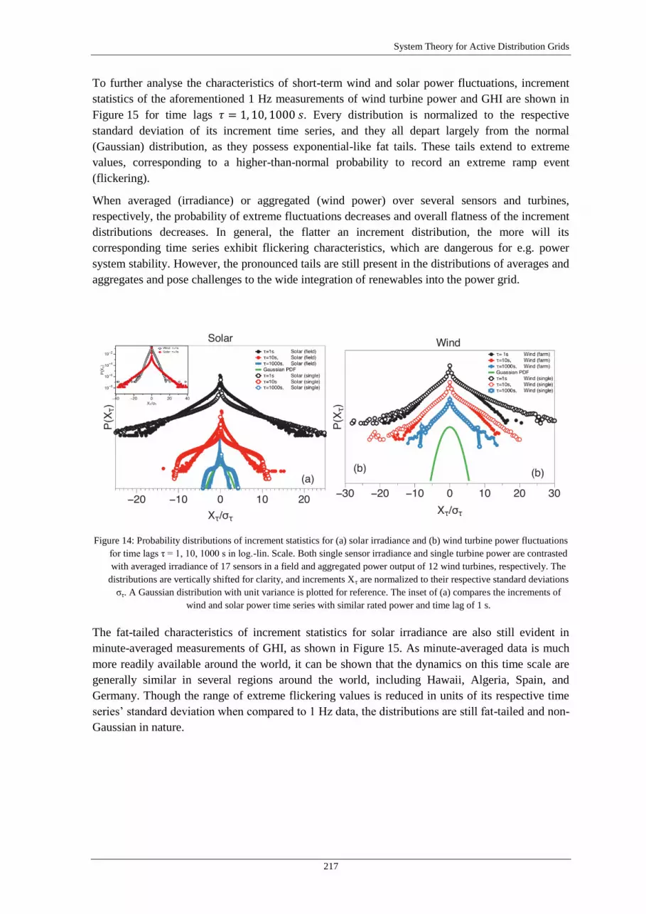
System Theory for Active Distribution Grids
217
To further analyse the characteristics of short-term wind and solar power fluctuations, increment
statistics of the aforementioned 1 Hz measurements of wind turbine power and GHI are shown in
Figure 15 for time lags 𝜏 = 1, 10, 1000 𝑠. Every distribution is normalized to the respective
standard deviation of its increment time series, and they all depart largely from the normal
(Gaussian) distribution, as they possess exponential-like fat tails. These tails extend to extreme
values, corresponding to a higher-than-normal probability to record an extreme ramp event
(flickering).
When averaged (irradiance) or aggregated (wind power) over several sensors and turbines,
respectively, the probability of extreme fluctuations decreases and overall flatness of the increment
distributions decreases. In general, the flatter an increment distribution, the more will its
corresponding time series exhibit flickering characteristics, which are dangerous for e.g. power
system stability. However, the pronounced tails are still present in the distributions of averages and
aggregates and pose challenges to the wide integration of renewables into the power grid.
Figure 14: Probability distributions of increment statistics for (a) solar irradiance and (b) wind turbine power fluctuations
for time lags τ = 1, 10, 1000 s in log.-lin. Scale. Both single sensor irradiance and single turbine power are contrasted
with averaged irradiance of 17 sensors in a field and aggregated power output of 12 wind turbines, respectively. The
distributions are vertically shifted for clarity, and increments Xτ are normalized to their respective standard deviations
στ. A Gaussian distribution with unit variance is plotted for reference. The inset of (a) compares the increments of
wind and solar power time series with similar rated power and time lag of 1 s.
The fat-tailed characteristics of increment statistics for solar irradiance are also still evident in
minute-averaged measurements of GHI, as shown in Figure 15. As minute-averaged data is much
more readily available around the world, it can be shown that the dynamics on this time scale are
generally similar in several regions around the world, including Hawaii, Algeria, Spain, and
Germany. Though the range of extreme flickering values is reduced in units of its respective time
series’ standard deviation when compared to 1 Hz data, the distributions are still fat-tailed and non-
Gaussian in nature.

Smart Nord Final Report
218
Figure 15: Probability distribution functions (PDF) of increment statistics for one minute averages of solar irradiance in
several regions around the world (Hawaii, Algeria (Sahara), Spain, Germany) for an increment time lag of 1 minute.
The distributions are vertically shifted for clarity, and increments Xτ are normalized to their respective standard
deviations στ. A Gaussian distribution with unit variance is plotted for reference. Extreme events of up to 20 σ are
recorded.
To dampen the high frequency flickering from multiple distributed wind and solar power systems,
we propose a time-delayed feedback method, which leads to a power feed-in time series of each
system according to equation Pi(t)new = (1 − α)Pi(t) + ϵP∗(t − T),(15 (see Material and Methods).
The optimal parameter values can be determined from minimization of, for example, the
aforementioned increment flatness. For the datasets analysed in this study, best increment flatness
is obtained for time delay lags 2 𝑠 < 𝑇 < 5 𝑠, while increment flatness decreases strongly with
increasing 𝛼. The optimal amplification coefficient is therefore considered to be around 𝛼 ≈ 0.5.
Figure 16a and b show how the flatness of increment statistics decreases from about 12.5 to about
6.5 for a wind park and an increment lag 𝜏 = 1 𝑠, while that of 17 averaged irradiance sensors
decreases from more than 120 to about 80 for the same increment lag. The larger the increment
time lag, the less pronounced the effect of time delayed feedback in general becomes for both wind
and solar power. The probability distributions of power increments for the aggregated wind
turbines and the averaged solar sensors are plotted in Figure 16c and d, respectively, for different
exemplary increment time lags. The positive suppression of strong non-Gaussian increment
statistics is evident, as the time-delayed distributions are both less flat, and both possess less
pronounced tails compared to their original counterparts.

System Theory for Active Distribution Grids
219
Figure 16: The results of time delayed feedback to suppress the short term flickering of wind and solar power. Panels (a-
d) show characteristic changes in stochastic dynamics of aggregated wind turbines and averaged solar sensors when
applying the time delayed feedback method: increment flatness (a, b) and probability distribution function of
increments (c, d). The suppression of extreme fluctuations are evident in all panels. The inset of panel (a) shows the
optimum values of delay lag T and amplification coefficient α of the time delayed feedback method with minimizing
the flatness of a 12 turbine wind farm for an increment lag 𝜏 = 2 𝑠. The inset of (b) shows typical variations in the
average irradiance of 17 sensors deployed in a field. The time delayed output is seen to exhibit smoother dynamics
than the untouched original data. The results presented in panels (a, c) are derived from 10000 s of 1 Hz data during a
time interval of strong intermittent fluctuations, as shown in inset of panel (c). Panels (b, d) are based on 1 Hz data of
a day with very variable cloud cover in Hawaii (03.03.2011), as shown in inset of panel (d).
4 Conclusion
In this work package, the characteristics of high frequency fluctuations in renewable power
production from wind turbines and photovoltaic systems have been analysed. First, a close
adherence to the well-known Kolmogorov-spectrum 𝑆(𝑓)~𝑓−5 3⁄ has been documented for more
than an order of magnitude in the power spectra of wind velocity, wind turbine power, and solar
irradiance. Then, the intermittent, non-Gaussian nature of solar irradiance and wind power
fluctuations has further been proven, by means of increment statistics, to feature strong stochastic
fluctuations (flickering) on time scales of seconds. Finally, a time delayed feedback method has
been proposed to help suppress this very flickering in distributed power generation.
These results imply that any distribution grid with local renewable power production is essentially
being fed with turbulent-like generation. The typical time scales for the associated stochastic
fluctuations in wind and solar power are in the range of seconds to minutes, and the more
decentralized wind or solar power systems are introduced to such a grid, the higher the magnitude

Smart Nord Final Report
220
of power fluctuations will become on these critical time scales. Despite a smoothing effect when
averaging, for example, several wind turbines, high frequency flickering still continues to occur
with a slightly reduced probability, but a higher magnitude in absolute numbers, of course.
Therefore, statistical analyses of the kind that have been presented here yield important information
that must be considered in order to guarantee an optimal design of resilient power grids. The
challenge will be to fine tune the intelligent management tools, as well as technological
possibilities, to achieve a stable and low cost power system that can handle the intermittent
renewable sources of power efficiently. The proposed time delayed feedback method aims to
contribute to reaching this goal by providing a means to suppress the most extreme short-term
flickering events in wind and solar power production at source.
As a consequence of the increased complexity in the power dynamics, any central management of
power grids is likely to become more and more difficult as the shares of wind and solar power
increase. Any means to accommodate intermittent renewable energy sources, and to mitigate risk
of grid instabilities will further increase the complexity of the existing systems, and thus, future
actions have to be based on the detailed knowledge of the dynamics of the variable power feed-in.
This type of research on power grid stability in the presence of stochastic renewable sources,
including their extreme events, is an emerging field of science. It forms a conjunction of several,
thus far disconnected fields of work and will allow for many more exciting results to come.

System Theory for Active Distribution Grids
221
Work Package 5.3: Demonstration Plant for MicroGrids under
Consideration of Islanding Detection
Benjamin Werther65
, Florian Pöschke65
and Hans-Peter Beck66
1 Introduction
Work package 5.3 has two main focuses. Part one improves a given experimental setup to a
demonstration plant for MicroGrids. The purpose of this demonstration plant is to validate the
theoretical results of the work packages of WP 5.1 and WP 5.2.
Furthermore this work package deals with the detection of islanding situations in MicroGrids. This
issue evolves from the on-going increase of distributed energy generation in the distribution grid.
This, from the islanding point of view, can be considered as threat for the safety since the
disconnectedness to the overlaid grid does not automatically ensure the volt-free state of the
operating devices. On the other hand this circumstance can be considered as chance to increase the
availableness of the devices in the distribution grid. Anyhow, in both of the mentioned aspects a
safe and sufficient fast detection of the transition from the grid-connected to the islanding mode of
the MicroGrid has to be ensured.
This work package considers several islanding detection methods, which are tested in the described
demonstration plant. The effectiveness of the different methods are compared in relation to real
measurements, where an islanding situation is enforced in the laboratory.
In addition different parameters for the identification of islanding situations in MicroGrids are
presented. Based on the measurement of the voltage in the grid, the frequency is obtained by a
phase-lock-loop. The frequency signal then is analysed with respect to the noise, which can provide
information of the state of the observed grid.
2 Demonstration Plant
The task in this part of the work package, is to improve the “FEN-Multi-VISMA-GRID”, a given
demonstration plant from the “Forschungsverbund Energie Niedersachsen (FEN)” [3]. In this
demonstration plant (cf. Figure 17) every device is connected on one single busbar. To analyse the
effect of decentralized power generation on power grids, a grid with line-elements is necessary.
These line-elements have to be scalable and combinable.
65
Clausthal University of Technology, 38678 Clausthal-Zellerfeld, Germany,
[email protected], Institute of Electrical Power Engineering and Energy Systems 66
Clausthal University of Technology, 38678 Clausthal-Zellerfeld, Germany,
[email protected], Institute of Electrical Power Engineering and Energy Systems

Smart Nord Final Report
222
Figure 17: realisation of the “FEN-Multi-VISMA-GRID”
It has been also added a central measurement system, to measure every line current and node
voltage with the same timestamp.
Figure 18 shows a possible example realization, in description from WP 5.1 and WP 5.2 can be
other realizations of the micro grid found.
Figure 18: Scheme of a possible realisation of the demonstration Plant
A schematic circut diagram of the line elements, is shown inFigure 19. Every line element is a
four-wire system, each wire has three switchable resistive and three switchable inductive elements.

System Theory for Active Distribution Grids
223
Figure 19: circuit diagram of a line element
3 Parameter of the Line Elements
The choice of the line elements is based on real data of typical cables, which are used in low
voltage distribution grids. In Table 2 parameter for different typical used cable of the low voltage
grid are shown. The line-elements should have a R/X-ratio between 1- 15. In low voltage grids the
typical line length is below 1 km and typical impedances are below 0.1 Ω. For an effect on the
voltage over the line elements, by small impedances like this, big currents are necessary. For this
reason every current is scaled by 1:10, by a voltage scaling factor 1:1. As a result the power is ten
times smaller compared to real distribution grids having the same voltage droop in the
demonstration plan.
Type R’ in Ω/km X’ in Ω/km R/X
16 mm² CU 1.15 0.077 14.9
150 mm² AL 0.206 0.068 3.0
240 mm² CU 0.078 0.067 1.2
Table 2: Parameter of typical lines in low voltage grids
This is realized with the following parameters (see Table 2). In Figure 20 is the voltage droop over
an in lab-scale ectypal 150 mm² AL line shown.
R1 0.50 Ω L1 433 µH
R2 0.24 Ω L2 216 µH
R3 0.10 Ω L3 108 µH
Table 3: Parameter of typical lines in low voltage grids

Smart Nord Final Report
224
Figure 20: Voltage droop over line elements with represented a 150 mm² AL line with different length
4 Measurement System
The choice of the measurement system is based on the identified requirements.
Resolution in Bit Resolution in V
8 3.125
12 0.2
16 12.2 m
18 3.05 m
Table 4: Voltage resolution in dependency of the ADC resolution
Each line element requires six measurements, and with eight elements, that implies that minimum
48 channels are needed for a full measurement. In the EN 61000-2-2 are compatibility
levels to the 50th harmonic (2.5 kHz) specified. To analyse up to this harmonic level is from
theoretical point of view a sampling rate more than 5 kHz per channel necessary. From a practical
point of view, 25 kHz per channel are necessary. The maximum ratings of the instantaneous
voltage are ±400 V, with a voltage converter with this maximum rating the voltage resolution in
dependency of the resolution of the ADC-card (Analog Digital Converter) can be found in Table 4.
In this table it can be seen that a resolution of 16 bit at least, because a discretisation error of 0.2
volts (at 12 bit) not being acceptable.
A measurement system which was chosen and fulfils this specification is a NI-PXe-1073 chassis
with three NI PXIe-6363 ADC-cards. A NI PXIe-6363 is a 16 bit ADC-Card with 16 differential
channels and cumulative sampling rate of 2 MS/s. This involve that the maximum resolution with
48 channels is 128 kHz, if a higher resolution is needed the number of the used channels has to be
reduced, till the maximum sampling rate is 2 MHz.
5 Islanding Detection
The steadily increasing percentage of decentralized energy generation in distribution grids leads to
new challenges concerning safety issues. Protection concepts of humans and operating devices
have to be reviewed. This tendency evolves from the fact of a change in the direction of the power
flow in electrical grids, cf. Figure 22. In the past massive power plants, which are connected to the
high voltage level of the electric transmission system, delivered the energy for the underlying parts

System Theory for Active Distribution Grids
225
of the electrical grid. Furthermore the power plants were responsible for the stable operation of the
grid, achieved by spinning reserve, primary and secondary control of the plants. Since the
decentralized energy resources (DER) have to contribute to the global stability of the grid, control
mechanism are included in the design of decentralized energy conversion systems. Thus the
likeliness of a formation of a stable grid without connection to the overlying high voltages level is
increased.
Figure 21: Grid structure islanding
Figure 22: Changing direction of the powerflow resulting from DER
On the other hand the high percentage of energy delivered by decentralized resources leads to the
possibility of increasing the availability in MicroGrids, especially in combination with energy
storage systems. In case of an islanding situation, the control strategy of the conversion systems,
either the ones for the decentralized resources or the ones for the storage systems, have to be
adjusted to the new MircoGrid situation, accordingly.
However, in any of the described cases the detection of an islanding situation has to be achieved
safe and sufficiently fast. There exist different concepts of the islanding detection in literature,
which can be divided into passive and active methods [1]. Since the tested islanding detection
methods will be compared to the here presented method based on the noise of the frequency signal
and passive methods have no influence on the quality of the electrical power supply of loads, only
passive methods are considered in this report.
6 Testing Islanding Detection Methods in the Demonstration Plant
Active components in MicroGrids usually watch over the frequency and voltage in the MicroGrid.
The acceptable bounds for the condition of the grid are defined in [2]. The frequency range has to

Smart Nord Final Report
226
fulfil 𝑓 = 50 𝐻𝑧 + 4 % /−6 % for 100 % of the time. The 10-minute average root mean square
value of the voltage has to remain in the bounds of 𝑈 = 𝑈𝑁 + 10 %/−15 % for all the time. So the
violation of these bounds (especially the frequency violation) would automatically imply an
islanding condition – or at least a problem of the grid itself – leading to a sage shutdown of the
active components or a change in the control scheme. Especially the frequency is compared to the
voltage, a global quantity being very stiff because of the wide spread leverage of the frequency all
over the transmission grid. The voltage can be altered depending on the point of measurement
throughout the considered MicroGrid and the power consumption/generation of the concerned
operating device. Since there can be active components in the MicroGrid, which are parameterised
to support the stable operation of the grid, the detection of a stable MicroGrid can become quiet
challenging and might not be separated from the grid-connected operation.
Figure 21 shows the structure of the demonstration plant for the islanding measurements. The
active components on the grid are represented by the virtual synchronous machine (VISMA)
connected to the grid by the switch S3, an inverter fed by a battery stack connected by S2 and a
synchronous machine (SG), which is directly mounted to the bus of the overlying grid. Opening the
switch S1 leads to an islanding of the MicroGrid. Depending on the structure of the grid, the
chosen parameters of the active components and the load a stable - in terms of voltage/frequency
limitations - MicroGrid in islanding mode can be achieved.
The synchronous generator is driven by an asynchronous machine fed by a frequency inverter. The
inverter can be parameterized, so a frequency dependent control is achieved. The possibly alterable
control properties are the proportional gain 𝑘𝑃 and the integration time constant 𝑇𝑖. The behaviour
of VISMA can be – as described in WP 5.1 – be altered through the quantities of 𝑘𝑑, 𝑇𝑑 and 𝐽. The
inverter used in the islanding experiment has a droop speed control 𝑘𝑓 to support the necessary
power generation to stabilize the grid.
In Figure 23 a measurement for the islanding of the presented MicroGrid can be seen. The
measurement of the three voltages and currents are captured in three different locations in the grid.
The black lines represent the measurement at the load, the green line shows the measurement at the
inverter and the black line considers the state at the bus with the overlying grid (until islanding
occurs) and the synchronous machine. As can be seen in Figure 23 a violation of the boundaries of
frequency and voltage did not occur, even though the islanding operation was enforced at 𝑡 ≈ 7 𝑠.
The inverter with speed droop control starts feeding in power as a result from the decrease of
frequency, leading to a stabilisation of the grid. As can be seen in Figure 23 the frequency and the
root mean square voltage remain in the defined bounds. Consequently the monitoring of these
quantities are not sufficient to identify an islanding situation. The measurements can be used to
create other signals indicating an islanding condition. Figure 23 takes the distortion, which includes
all frequencies with a magnitude above 2 V (to exclude the measurement noise), the rate of change
of Voltage 𝑑𝑈𝑒𝑓𝑓
𝑑𝑡 and the rate of change of power
𝑑𝑃
𝑑𝑡 into account. The voltage can be viewed as a
vector with phase, magnitude and frequency. The islanding results in a change of this vector, which
can be seen in the frequency, magnitude (here rms-value), angular acceleration (rate of change of
frequency) and the phase. Anyhow this event occurs only once and might not be distinguished from
a change of load, whereas the distortion shows a permanent change and thus indicates the islanding
situation.

System Theory for Active Distribution Grids
227
Parameter Quantity
𝑘𝑃 3
𝑇𝑖 0.5 s
𝑘𝑓 1000 W/Hz
load 3400 W
Table 5: Parameter for stable islanding
Table 5 shows the Parameters used for this stable operation of the MicroGrid. The switch S3 was
opened in this particular measurement; anyhow a stable islanding operation can also achieved by
the use of the VISMA in different experiments.
Figure 23: Measurement Islanding of the MicroGrid
7 Islanding Detection Based on the Frequency Dynamics
As shown in Figure 23, the dynamics of the voltage vector change due to the altered operation in
islanding mode. Through the use of a phase locked loop the frequency signal can be obtained. It
can be observed, that in islanding situation the statistical parameters of the frequency signal
changes. One of the parameters, which showed a good level of identification of the grid situation,
was the sum of the squares of differences in the frequency signal, defined by equation (16).
𝑺𝑸𝑫(𝐧) = ∑(𝒇(𝒊) − 𝒇(𝒊 + 𝟏))𝟐
𝐧−𝟏
𝒊=𝟏
(16)
This identification is based on the idea of a very large amount of switching loads and generators in
the global grid, which directly influences the frequency in a very short time scale. Thus the
frequency signal is used to generate the SQD for n discrete measured points. The number of the
measured points in combination with the sample time defines the identification time.

Smart Nord Final Report
228
Figure 24: SQD of different devices, green: VISMA, red: grid; purple/blue: synchronous machine
Especially the possibility of identification of the participating utilities leads to the islanding
detection. It can be shown, that different participants show a very unique level of SQD, when being
active in the MicroGrid. When the overlying grid is considered as a component, cf. Figure 21, the
high number of loads of the overall grid affect the frequency signal in a unique way, compared to
other devices like the synchronous machine or the VISMA. In Figure 24 the measurement of the
SQD for different devices are shown. The green line shows the SQD for a grid, where only the
VISMA is active. The red lines represent the grid connected operation of the MicroGrid, whereas
the purple/blue lines show a grid driven by synchronous machines.
Some facts are important for the design of SQD generation. First of all the dynamics of the
frequency signal depends on the parameters of the used phase-locked-loop (PLL). On the other
hand the frequency is filtered through a high pass before forwarded to the PLL, since the slowly
changing components (ca. seconds - minutes) do not the affect the SQD signal, which has a high
dependence on the sample time of the measurement.
Figure 25: Frequency dependent magnitude of different generators
Furthermore this method can be improved by the use of frequency dependent analysis. It can be
shown, that the frequency demodulated signal (by the use of a PLL) behaves unique dependent on
the investigated frequency bounds. Figure 25 shows the frequency dependent magnitudes of a
synchronous machine (SM) on the left side and 3-phase inverter (WR2) on the right side of the
figure. Using this knowledge, the generation of the SQD can be specified in certain bounds, cf
Measurement no.

System Theory for Active Distribution Grids
229
Figure 26. It shows the analysed SQD for different generators (SM=synchronous machine,
Netz=grid, WR1/2/3=inverter) from a frequency of f=400 Hz upwards.
Figure 26: SQD, frequency sensitive from a frequency f=400 Hz
8 Conclusion
Parameters of a VISMA have been optimized to get a desired behaviour of the output power. The
simulated and the measured results from the laboratory agree well for an optimal parameter setting.
In an extension, a MicroGrid has been optimized with respect to the parameters of a VISMA which
is part of the MicroGrid. First results show that with the change of the two free parameters in the
cost functional the focus of the optimization can be changed. In the future, one should think of a
optimization method from statistical physics to find global minima more likely than with the simple
Downhill-Simplex method. A concept for distributed frequency control for MicroGrids has been
presented and validated via simulations. In this set-up, three VISMA-controlled inverters
communicate with each other to restore an original load sharing. This works well and also the
frequencies of the VISMAs could be harmonized. The characterization of very resilient network
topologies has been done for two different models. For these models, resilient networks have many
edges and a small diameter. A third model which deals with the “maximum-disturbance” stability
could be considered for investigation.
An optimization method to use less free parameters of the decentralize devices to get in sum the
desired behaviour in the grid is confirmed. Also a method to investigate the influence of topologies
of grids on different stability measures was developing.
A decentralized frequency controller for island mode with a zero steady-state error and projectable
load sharing was elaborated. In case of a stable island mode, it’s important to detect the situation.
Because the control strategies has to change or for safety reasons devices had to been shut down.
As the characteristics of high frequency variability in decentralized power production from wind
turbines and photovoltaic systems are shown to be turbulent-like, with non-Gaussian increment
statistics, distribution grids need to be prepared for an increasing amount of intermittent power
feed-in. The frequent occurrence of strong stochastic fluctuations (flickering) in the renewables
calls for new measures, like the proposed time delayed feedback method, to be developed and
implemented in future MicroGrids in order to ensure stability in voltage and frequency, and to
guarantee the meeting of power demand. These tasks will become more urgent and more
challenging, the higher the shares of decentralized wind and solar power become.
Islanding detection methods and their applicability in MicroGrids was tested. It could be shown
that methods which are based on off-limit conditions had no reliable results. The procedures which
carry out a continuous assessment of the state variables seem more useful.

Smart Nord Final Report
230
A demonstration plant for MicroGrids was build up. The purpose of this demonstration plant was to
validate the theoretical results of the work, and it is available for further research activities.
References
[1] W. Bower, M. Ropp, “Evaluation of Islanding Detection Methods for Utility-Interactive Inverters in
Photovoltaic Systems,” Sandia National Laboratories, Albuquerque, New Mexico 87185, 2002.
[2] Voltage characteristics of electricity supplied by public distribution networks; German version EN
50160:2010+Cor.:2010.
[3] Y. Chen, R. Hesse, D. Turschner, H.-P. Beck, “Untersuchungen an der VISMA (TP 11),
Forschungsverbund Energie Niedersachsen Abschlussbericht,” Braunschweig 2012. ISBN: 978-3-
925268-45-8.
[4] Y. Chen, R. Hesse, D. Turschner, H.-P. Beck, “Investigation of the Virtual Synchronous Machine in
the Island Mode,” 3rd IEEE PES Innovative Smart Grid Technologies Europe (ISGT Europe),
Berlin, 2012.
[5] J. Nelder, R. Mead, “A Simplex method for function minimization,” Computer Journal 7, 308 (1965)
[6] K. Hukushima, K. Nemoto, “Exchange monte carlo method and application to spin glass simulations,”
J. Phys. Soc. Jpn., 65:1604 (1996).
[7] W. Heins, T. Dewenter, A. K. Hartmann, C. Bohn, “Parameter optimization of a virtual synchronous
machine in a MicroGrid,” in preparation.
[8] J. W. Simpson-Porco, F. Dörfler, F. Bullo, “Synchronization and power sharing for droop-controlled
inverters in islanded microgrids,” in Automatica 49 (2013), Nr. 9, pp. 2603–2611.
[9] T. Dewenter, B. Werther, A. K. Hartmann, H.-P. Beck, “Optimierung des dynamischen Verhaltens
netzstützender Anlagen am Beispiel der Virtuellen Synchronmaschine,” Graz/Austria, 12.-14. Februar
2014, 13. Symposium Energieinnovation.
[10] A. K. Hartmann, “Sampling rare events: Statistics of local sequence alignments,” Phys. Rev. E, 65,
056102 (2002).
[11] A. K. Hartmann, “Large-deviation properties of resilience of transportation networks,” Eur. Phys. J B
87, 114 (2014).
[12] T. Dewenter, A. K. Hartmann, “Large-deviation properties of resilience of power grids,” New J. Phys.
17, 015005 (2015).
[13] A. K. Hartmann, B. Werther, W. Heins, T. Dewenter, “Large-deviation study of the maximum-
disturbance stability of power grids,” in preparation.
[14] E. J. Davison, E. M. Kurak, “A Computational Method for Determining Quadratic Lyapunov
Functions for Non-linear Systems,” Automatica, Vol. 7, pp. 627-636. Pergamon Press, 1971.
[15] J. Carrasco, L. Franquelo, J. Bialasiewicz, E. Galvan, R. Guisado, M. Prats, J. Leon, N. Moreno-
Alfonso, “Power-electronic systems for the grid integration of renewable energy sources: A survey,”
Industrial Electronics, IEEE Transactions on, vol. 53, no. 4, pp. 1002–1016, Jun. 2006.
[16] L. von Bremen, “Large-scale variability of weather dependent renewable energy sources,” in
Management of weather and climate risk in the energy industry. Springer, 2010, pp. 189–206.
[17] F. Blaabjerg, Z. Chen and S. B. Kjaer, “Power electronics as efficient interface in dispersed power
generation systems,” Power Electronics, IEEE Transactions on 19 1184, 2004.
[18] J. Marcos, O. Storkel, L. Marroyo, M. Garcia, E. Lorenzo, “Storage requirements for PV power ramp-
rate control,” Solar Energy 99, 28, 2014.
[19] J. Marcos, I. de la Parra, M. Garcia, L. Marroyo, “Control Strategies to Smooth Short-Term Power
Fluctuations in Large Photovoltaic Plants Using Battery Storage Systems,” Energies 7, 6593, 2014.
[20] M. Fontoynont, et al., “Satellight: a WWW server which provides high quality daylight and solar
radiation data for Western and Central Europe.” Proceedings of the 9th Conference on Satellite
Meteorology and Oceanography. No. 2, 1998.
[21] A. Woyte, R. Belmans, J. Nijs, “Fluctuations in instantaneous clearness index: Analysis and
statistics,” Solar Energy 81, 195, 2007.
[22] M. Amin, “Energy: The smart-grid solution,” Nature, 499, 145, 2013.
[23] P. Milan, M. Wächter, J. Peinke, “Turbulent Character of Wind Energy,” Phys. Rev. Lett., 110,
138701, 2013.

System Theory for Active Distribution Grids
231
[24] A. Nieße, M. Tröschel, M. Sonnenschein, “Designing dependable and sustainable Smart Grids -How
to apply Algorithm Engineering to distributed control in power systems,” Environmental Modelling &
Software 56, 37, 2014.
[25] R. Baldick, et al., “Initial review of methods for cascading failure analysis in electric power
transmission systems,” IEEE PES CAMS task force on understanding, prediction, mitigation and
restoration of cascading failures, IEEE Power Engineering Society General Meeting, 10142341, 1,
2008.
[26] B. A. Carreras, V. E. Lynch, M. L. Sachtjen, I. Dobson, D. E. Newman, “Modeling Blackout
Dynamics in Power Transmission Networks,” Hawaii International Conference on System Sciences,
January 3-6, Maui, Hawaii, 2001.
[27] I. Dobson, B. A. Carreras, V. E. Lynch, D. E. Newman, “Complex systems analysis of series of
blackouts: cascading failure, critical points, and self organization,” Chaos, 17(2), 026103, 2007.
[28] G. Nicolis, I. Prigogine, “Exploring Complexity,” W. H. Freeman, San Francisco, 1989.
[29] B. A. Carreras, D. E. Newman, I. Dobson, A. B. Poole, “Evidence for self-organized criticality in a
time series of electric power system blackouts,” IEEE Trans. Circuits & Systems I 51, 1733, 2004.
[30] M. Rohden, A. Sorge, M. Timme and D. Witthaut (2012) Self-Organized Synchronization in
Decentralized Power Grids, Phys. Rev. Lett. 109, 064101.
[31] D. Witthaut, M. Timme, “Braess’s paradox in oscillator networks, desynchronization and power
outage,” New J. Phys. 14, 083036, 2012.
[32] M. Chertkov, M. Stepanov, F. Pan, R. Baldick, “Exact and Efficient Algorithm to Discover Extreme
Stochastic Events in Wind Generation over Transmission Power Grids,” 2011.
[33] J. Heitzig, N. Fujiwara, K. Aihara, J. Kurths, “Interdisciplinary challenges in the study of power grid
resilience and stability and their relation to extreme weather events,” in Eur. Phys. J. Special Topics
223(12), 2281, 2014.
[34] C. Kamath, “Understanding wind ramp events through analysis of historical data,” in Transmission
and Distribution Conference and Exposition, IEEE PES,1, 2010.
[35] H. Haken, “Advanced Synergetics, Instability hierarchies and self-organizing systems and devices,”
Springer, Berlin, 1983.
[36] R. Friedrich, J. Peinke, M. Sahimi, M. R. Rahimi Tabar, “Approaching complexity by stochastic
methods: From biological systems to turbulence,” Phys. Rep. 506, 87, 2011.
[37] C. Nicolis, V. Balakrishnan, G. Nicolis, “Extreme Events in Deterministic Dynamical Systems,” Phys.
Rev. Lett. 97, 210602, 2006.
[38] Extreme Events in Nature and Society, Edited by: S. Albeverio, V. Jentsch & H. Kantz (2006)
Springer, Berlin.
[39] H. Farhangi, “The Path of the Smart Grid,” IEEE Power and Energy Magazine 8, 18, 2010.
[40] H. Kanchev, D. Lu, F. Colas, V. Lazarov, B. Francois, “Energy Management and Operational
Planning of a Microgrid With a PV-Based Active Generator for Smart Grid Applications,” IEEE
Transactions on Industrial Electronics 58, 4583, 2011.
[41] H. Haken, “Synergetics: Introduction and Advanced Topics,” Springer, Berlin, 2004.
[42] S. V. Buldyrev, R. Parshani, G. Paul, H. E. Stanley, S. Havlin, “Catastrophic cascade of failures in
interdependent networks,” Nature 464, 1025, 2010.
[43] P. J. Menck, J. Heitzig, N. Marwan, J. Kurths, “How basin stability complements the linear-stability
paradigm,” Nature Physics 9, 89, 2013.
[44] P. Menck, J. Heitzig, J. Kurths, H. J. Schellnhuber, “How dead ends undermine power grid stability,”
Nat. Commun. 5, 3969, 2014.
[45] R. Perez, T. Hoff, J. Dise, D. Chalmers, S. Kivalov, “The cost of mitigating short-term PV output
variability,” Energy Procedia 57 755, 2014.
[46] A. Engler, “Applicability of droops in low voltage grids,” International Journal of Distributed Energy
Resources, Vol 1, No 1, 2005.
[47] P. Kundur, N. J. Balu, M. G. Lauby, “Power system stability and control,” McGraw-Hill: New York,
1994.
[48] W. Heins, C. Bohn, “Distributed frequency control in MicroGrids based on the virtual synchronous
machine,” in preparation.


SmartSpatial
233
Sub-Project Six:
SmartSpatial


SmartSpatial
235
SmartSpatial
Claudia Palmas67
, Almut Siewert67
, Francesca Dossola67
, Christina von Haaren67
and Michael Rode67
Abstract
In the context of energy transition, Germany’s political agenda on renewable power usage aims at further
expansion of decentralized energy production, in a large scale. However, the large-scale installation and
utilization of decentralized renewable energy technologies necessitates relevant changes of all sectors of
energy use and the transformation of the energy system. These changes can lead to negative impacts on the
landscape and such expansion is often accompanied by land use conflicts and environmental sensitivity due
to disturbance. Moreover, a chaotic development of renewable energy (RE) can exacerbate conflicts with
residents, nature conservation, tourism interests, and food production. Therefore, rational approaches to
spatial planning are needed for a sustainable allocation of renewable energy systems. In SP 6 we develop a
smart and spatial model (SmartSpatial) in order to identify the most suitable areas for decentralized RE
generation, which can be integrated into smart and in particular into micro grids [SP 1-5]. SmartSpatial is
based on a spatial multi-criterial methodological framework for RE siting. It follows the objectives of
sustainability by simultaneously maximizing spatial efficiency and minimizing the environmental impacts of
RE production. The model supports decisions on regional RE target setting and siting by combining the
spatial efficiency of using the RE potential and projected environmental impacts. Methodologically, the
model combines RE-potential analysis with an ecological impact analysis, which is specified for different RE
specific pressure factors. Firstly, we estimate different GIS-based theoretical energy potentials (wind, solar,
and biomass), whereby the mapping estimation depends only on the geophysical properties of the landscape.
Accordingly, we develop a raster data-set to estimate the technical energy potentials by including the
technical requirements of the different power plants [WP 6.1]. In order to exclude unsuitable areas, we
identify institutional based (legally) and recommended (in the practice considered) restriction areas. In
parallel, on the basis of regional data about environmental values and sensitivities to typical pressures caused
by RE-production, a map of spatially differentiated degrees of environmental trade-offs is produced for a
region [WP 6.2]. Finally, we overlay the three GIS-based outcomes (layers) in order to compare the specific
and combined energy production by developing different scenarios for identifying suitable and conflict areas
for RE-development [WP 6.3]. These outcomes are compared with the actual decision-space for RE-
development and the political RE energy targets. This approach supports participative and more transparent
regional planning and decision processes in order to find the most environmental sustainable options of RE-
development with the highest energy potentials in a given region. Furthermore, due to the high model’s
feasibility, local preferences can be integrated into site selections for RE expansions. The possibility to test
different scenarios as well as the transparency of trade-offs between energy output and the environment,
make the model a suitable instrument for decision processes of municipalities and the public on the regional
or higher decision levels. The model is tested in the Hanover region in Lower Saxony, but could be also
applicable in other German or European regions if it were to be slightly adjusted according to the availability
of local data.
1 Introduction
In the context of energy transition, the political agenda in Germany regarding renewable power
usage intends to increase the share of renewable energy (RE) in final electricity consumption to at
least 80 % by 2050 [1]. However, the large-scale installation and utilization of decentralized
renewable energy technologies compels relevant changes be made to all sectors of energy use and
the transformation of the energy system. The energy system is currently changing from “energy for
67
Leibniz Universität Hannover, 30149 Hanover, Germany,
[email protected], Institute of Environmental Planning

Smart Nord Final Report
236
space” to “energy from space” [2]. These changes can lead to negative impacts on the landscape as
expansion is often accompanied by land use conflicts and environmental sensitivities to disturbance
[3], [4], [5], [6], [7]. Moreover, a chaotic development of renewable energy (RE), especially due to
the initial largely unregulated implementation of the different types of RE facilities, can exacerbate
conflicts with residents, nature conservation, tourism interest and food production [8], [9], [10].
Consequently, public protests against wind power plants, electricity grids, or increases in maize
cultivation are, in spite of the German public, largely supported Transformation of the Energy
System (“Energiewende”) and have become common in many regions [11], [12], [13], [14]. Even
though many regions have set themselves ambitious RE production targets, current planning
practice do not yet include an integrated analysis of RE production and an effective evaluation of
energy-related land-use issues. However, sectorial approaches are not sufficient when dealing with
the aforementioned issues [8], [10], [15], [16]. Instead, it is necessary to estimate GIS-based RE-
potentials, as input data for decentralized RE generation [17], [18], and to minimize the land
consumption for RE production on the regional and local scale [10], [15], [16], [19]. This can be
achieved by the optimal exploitation of combined RE potentials together with a simultaneous
minimization of environmental trade-offs [6], [10], [16]. Therefore, rational approaches to spatial
planning are needed for decentralized RE-generation. Approaches, which can be integrated into
smart and in particular, into micro grids for an intelligent energy supply by different sources
[SP 1-5]. A spatial methodological framework should be further developed to integrate the
objectives of decentralized energy generation, spatial energy efficiency, and sustainable landscape
planning and development [16], [17], [18], [20].
2 Research Questions
In order to support regions in achieving their energy targets and an environmentally friendly way to
attain decentralized RE-production in the future, we aim to answer the following research
questions:
How can the geographic distribution of different energy potentials (wind, solar, and biomass
energy) be calculated on the regional scale? Which criteria and algorithms are needed for
identifying the theoretical and technical energy potentials? How can RE energy mix
combinations be identified? [WP 6.1]
How can environmental values and sensitivities, opposed RE production, be integrated on the
regional scale? Which methods are suitable for modelling the value of natural resources and
their environmental sensitivity to disturbance? [WP 6.2]
According to energy potential estimations and environmental assessments, how can suitable
areas for RE-production be identified? Which kind of scenarios can be developed in order to
support political decisions by optimizing the space energy efficiency and minimizing
environmental trade-offs? [WP 6.3]
Do the results increase the scope for decision making for RE generation in comparison to the
current formal approach that is based on legal and planning standards? Do the results help to
achieve the RE political regional targets by 2050? [WP 6.3]
3 Methods and Materials
We sought to solve the above research questions by developing the SmartSpatial model as a system
for analysing and optimizing different RE scenarios. SmartSpatial is based on a spatial multi-
criterial methodological framework for RE siting. It follows the objectives of sustainability by
simultaneously maximizing the spatial efficiency and minimizing the environmental impacts of RE

SmartSpatial
237
production (Figure 1). Methodologically, the model combines RE-potential analysis with an
ecological impact analysis, which is specified for different RE pressure factors. The model consists
of three modules: a first raster data-set of GIS-based theoretical energy potentials (wind, solar, and
biomass), whereby the mapping estimation depends only on geophysical properties of the
landscape; and a second raster data-set of GIS-based technical energy potentials, whereby technical
requirements of the different power plants are included [WP 6.1]. The second module makes
assessments based on regional data environmental values and sensitivities against typical pressures
caused by RE-production. Accordingly, we produce a map of spatially differentiated degrees of
environmental trade-offs. In order to exclude unsuitable areas, institutional established (legally)
and recommended (in the practice considered) restriction areas are identified [WP 6.2]. The third
module is obtained by overlaying the three GIS-based outcomes (layers) in order to compare the
specific and combined energy production. Different scenarios are developed for identifying suitable
and conflict areas for RE-development [WP 6.3]. These outcomes are compared with the actual
decision-space for RE-development and the political RE energy targets.
Figure 1: Methodological framework of SmartSpatial
In order to test the modules with respect to plausibility of results and their applicability under
actual spatial data conditions, SmartSpatial is applied in the region of Hanover in Lower Saxony.
This region is chosen as a case study area for the project, on account of the high interest and
engagement in RE-development in the areas and because of the comparatively comprehensive
digital geo-data attached to its recently updated regional landscape plan [21], [22].
Administratively, the region of Hanover is composed of 21 municipalities and townships spreading
across 2,290 km². With Lower Saxony’s capital city Hanover situated at its centre, the region is the
most densely populated (496 inhabitants per km²) area within the federal state (166 inhabitants per
km²) [23]. The complexity associated with the increasing urban sprawl of suburbanization, includes
traffic growth and road expansions, the interests of nature conservation, agriculture and tourism,
and growing RE-development. Dealing with each of these various issues contributes to the
ambitious challenges facing regional planning. In fact, as a 100 % RES Region, Hanover aims to
reduce GHG emissions by 95 % while cutting down on 50 % of final energy consumption [24].
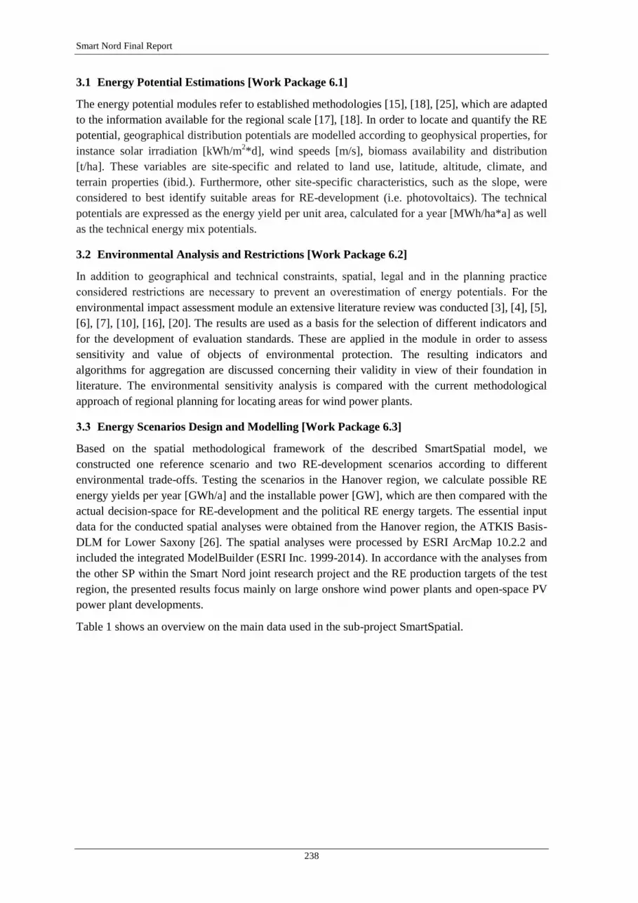
Smart Nord Final Report
238
3.1 Energy Potential Estimations [Work Package 6.1]
The energy potential modules refer to established methodologies [15], [18], [25], which are adapted
to the information available for the regional scale [17], [18]. In order to locate and quantify the RE
potential, geographical distribution potentials are modelled according to geophysical properties, for
instance solar irradiation [kWh/m2*d], wind speeds [m/s], biomass availability and distribution
[t/ha]. These variables are site-specific and related to land use, latitude, altitude, climate, and
terrain properties (ibid.). Furthermore, other site-specific characteristics, such as the slope, were
considered to best identify suitable areas for RE-development (i.e. photovoltaics). The technical
potentials are expressed as the energy yield per unit area, calculated for a year [MWh/ha*a] as well
as the technical energy mix potentials.
3.2 Environmental Analysis and Restrictions [Work Package 6.2]
In addition to geographical and technical constraints, spatial, legal and in the planning practice
considered restrictions are necessary to prevent an overestimation of energy potentials. For the
environmental impact assessment module an extensive literature review was conducted [3], [4], [5],
[6], [7], [10], [16], [20]. The results are used as a basis for the selection of different indicators and
for the development of evaluation standards. These are applied in the module in order to assess
sensitivity and value of objects of environmental protection. The resulting indicators and
algorithms for aggregation are discussed concerning their validity in view of their foundation in
literature. The environmental sensitivity analysis is compared with the current methodological
approach of regional planning for locating areas for wind power plants.
3.3 Energy Scenarios Design and Modelling [Work Package 6.3]
Based on the spatial methodological framework of the described SmartSpatial model, we
constructed one reference scenario and two RE-development scenarios according to different
environmental trade-offs. Testing the scenarios in the Hanover region, we calculate possible RE
energy yields per year [GWh/a] and the installable power [GW], which are then compared with the
actual decision-space for RE-development and the political RE energy targets. The essential input
data for the conducted spatial analyses were obtained from the Hanover region, the ATKIS Basis-
DLM for Lower Saxony [26]. The spatial analyses were processed by ESRI ArcMap 10.2.2 and
included the integrated ModelBuilder (ESRI Inc. 1999-2014). In accordance with the analyses from
the other SP within the Smart Nord joint research project and the RE production targets of the test
region, the presented results focus mainly on large onshore wind power plants and open-space PV
power plant developments.
Table 1 shows an overview on the main data used in the sub-project SmartSpatial.

SmartSpatial
239
Energy potentials
So
lar
Inputs Scale/unit/format Sources
Digital Terrain
Model (DTM) 50 m x 50 m
State Office of geographic information and land
development (“Landesamt für Geoinformation
und Landentwicklung”, LGLN)
Aspect (azimuth of
the solar panel) 180°
Geographic Resources Analysis Support System
(GRASS GIS) manual, 2012
Slope (solar panel
inclination) 37°
GRASS GIS manual, 2012
Linke atmospheric
turbidity coefficient 3.0 - 4.2
GRASS GIS manual, 2012
Albedo coefficient 0.2 GRASS GIS manual, 2012
Real-sky beam
radiation coefficient 0.118 - 0.62
GRASS GIS manual, 2012
Real-sky diffuse
radiation coefficient 0.86 - 5.49
GRASS GIS manual, 2012
Day of the year 1 - 365 [d] GRASS GIS manual, 2012
PVGIS Database [kWh/m²]
Photovoltaic Geographical Information System
Interactive Maps (Joint Research Center of the
European Commission, JRC, 2010).
Win
d
Digital Terrain
Model (DTM) 50 m x 50 m
State Office of geographic information and land
development (“Landesamt für Geoinformation
und Landentwicklung”, LGLN)
Wind speeds [dm/s] German Weather Service (“Deutscher
Wetterdienst”, DWD), 1981-2000
Bio
ma
ss
Biomass (maize)
yields [t/ha] Bauböck, Kapas, Uni Göttingen, 2012
Environmental sensitivities and values
RE
Basic geodata 1:25,000
State Office of geographic information and land
development (“Landesamt für Geoinformation
und Landentwicklung”, LGLN)
Information for
environmental
indicators
1:50,000
Regional planning programme (“Regionales
Raumordnungsprogramm”, RROP), Hanover
region, 2005
Geodata on abiotic
and biotic
environment
1:50,000
Landscape structure plan
(“Ladschaftsrahmenplan”,LRP), Hanover
region, 2013
Geodata on soil
charateristics 1:25,000
State Office of Mining, Energy and Geology,
“Landesamt für Bergbau, Energie und
Geologie”, LBEG, 2015
Environmental
protected areas 1:50,000
Department for environment, energy and
climate protection of Lower Saxony
(“Niedersächsisches Ministeriums für Umwelt,
Energie und Klimaschutz”, MU)
Priority areas for
wind development
and recreation areas
1:50,000 Regional plan (“Regional Plan”, RP), Hanover
region, 2005
Table 1: Input data for the energy potential estimation and the environmental analysis

Smart Nord Final Report
240
The current restrictions for RE-development are derived from either legally binding regulations
such as laws (e.g. Germany’s Federal Nature Conservation Act, BNatSchG) that are referred to as
hard restriction areas, or from different recommendations by official planning institutions and are
referred to as soft restriction areas (Table 2 and Table 3). In the case of regulations on wind power
development, we refer to the latest draft of the Wind Energy Decree, produced by the federal state
of Lower Saxony (“Windenergieerlass”) [28].
Area Categories Wind
Power PV Plants Energy Maize Legal Basis
Bu
ild
ing
are
as
Residential areas hard - hard
§5 BlmSchG; §35
BauGB
400 m residential area’s buffer
zone hard - -
§5 BlmSchG; §35
BauGB
Commercial and industrial areas hard - -
§5 BlmSchG; §35
BauGB
400 m commercial and industrial
area’s buffer zone hard - -
§5 BlmSchG; §35
BauGB
Infr
ast
ruct
ure
s
Motorways, 30 m hard - §35 BauGB
40 m motorway’s buffer zone hard - -
§9 FStrG; §24
NStrG
Federal roads, 16 m hard - §35 BauGB
20 m federal road’s buffer zone hard - -
§9 FStrG; §24
NStrG
Overhead power lines, 31m hard - - DIN EN 50341-3-5
82 m overhead power line’s
buffer zone hard - - DIN EN 50341-3-5
Wa
ter a
nd
so
il
(all) Water surfaces - - hard -
Main watercourses, 50 m buffer
zone hard - - §61 BNatSchG
Flood hazard areas hard hard -
§78 WHG; §35
BauGB
Slopes >21 % - soft - -
Areas of high water erosion pot. - - soft -
Areas of high wind erosion pot. - - soft -
Table 2: A general overview on the restriction areas for RE-development; - = no restrictions and
legal basis [16], [27] - [30]

SmartSpatial
241
Area Categories Wind
Power PV Plants Energy Maize Legal Basis
Pro
tecte
d a
rea
s
Nature conservation areas hard hard hard §23 BNatSchG
EU-Special Protection Areas
(SPA) hard soft soft §31 BNatSchG
Protected biotopes hard hard hard §30 BNatSchG
Protected landscape units hard hard hard
§28, §29
BNatSchG
Drinking water protection areas
(zone I and II) hard - hard §51 WHG
Drinking water protection areas
(zone III) - - soft -
Landscape conservation areas soft soft - -
Special areas of conservation
(FFH) soft soft soft -
Bio
div
ersi
ty,
flo
ra a
nd
fa
un
a
Faunisic habitats (values 4 and
5) - soft soft -
Migratory bird resting areas
(values 3-5) soft soft soft -
Wetlands of international
importance soft soft soft -
Breeding bird habitats (values 3-
5) soft - - -
Bat habitats soft - - -
Areas of special importance für
species and ecosystems - soft - -
Forests soft soft soft -
Green belts and infrastructures - soft - -
La
nd
sca
pe
Landscape units of special
importance soft soft soft -
Landscape of special structural
diversity - soft - -
Areas of historical-cultural
importance - soft - -
Table 3: A general overview on the restriction areas for RE-development; - = no restrictions and
legal basis [16], [27] - [30]
4 Renewable Energy Potentials [Work Package 6.1]
Based on the geo-physical properties, we estimate theoretical RE potentials for wind power, solar
power, and biomass cultivation for the production of biogas. Subsequently, by taking into account
the technical requirements, we develop different GIS-based raster data-sets in order to compare and
combine different energy yields (Figure 2). These results are used as input-data to model energy
RE-development scenarios for the Hanover region.

Smart Nord Final Report
242
Figure 2: General methodological procedure for identifying preliminary scenarios for RE-development according to GIS-
based RE-potentials
5 Spatial Wind Energy Potential
Theoretical wind energy potentials are estimated by processing data on average annual wind speeds
derived from the German Weather Service (“Deutscher Wetterdienst”, DWD). These input data
from DWD for the reference period 1981 to 2000 exhibit wind speeds at 10m height above ground
at a 200m resolution. These data were already processed taking into account roughness (from relief
and land characteristics), height above sea level, as well as geographical location. Differences
between calculated and measured wind speeds are quoted ± 0.15. We further processed these input
data by firstly downscaling on a Digital Terrain Model, DTM (50), and secondly calculating wind
speeds at the heights of 65, 100, 140, and 180 m. For the further analyses, we used a wind speed at
the height of 100 m, accounting for wind power plants of current technical standard. The increases
of wind speed at the different heights are calculated by equation 1 (Eq.1). Underlying assumption is
that the atmosphere thermic condition is stable, which is expressed by the empirically derived
coefficient α at a value of α = 0.143 [31], [32].
(Eq.1) v = vref (z / zref) α
Where:
v: wind speed at height z above ground level;
vref: reference speed, i.e. a wind speed we already know at height zref;
z: height above ground level for the desired velocity, v;
zref: reference height, i.e. the height where the wind speed is measured vref.
In order to obtain the wind technical energy potential expressed in energy yields per unit area,
calculated for a year [MWh/ha], we take into account a “standard” wind turbine with an installable
power of 3 MW. For each installed turbine, an average distance of about 300 m is needed.
Therefore, we consider for the calculation, a grid of 300 m × 300 m. The fundament of each turbine
occupies a raster cell of approximately 20 m × 20 m. We excluded a buffer zone of about
90,000 m2 around each wind turbine which cannot be occupied by other wind turbines. Energy
SmartSpatial
243
yields vary according to average wind speeds distribution for each cell throughout the region. Due
to data unavailability, we do not take into account the wind speeds variability on the region.
5.1 Spatial Solar Energy Potential
Theoretical solar energy potentials are estimated on the basis of a DTM (50) in raster map format.
For this purpose, the open-source solar radiation tools r.sun solar radiation model, implemented in
GRASS GIS (6.4.2) and the PVGIS CM-SAF estimation utility are used [33]. The calculation of
the solar radiation for specific sites is based on data taken from the PVGIS database, which
includes the crucial influencing factor of sky cloud coverage, with a stated overall error of
approximately 5 % for an entire year [18]. Clear sky indexes are estimated by the JRC [34]. As an
approximation, the assumption was made that albedo and Linke turbidity are constant during each
month for the entire Hanover region. The output raster map expresses the annual average of global
irradiation daily sums estimated for optimized angle [kWh/m2*d].
Defining the solar technical potentials we consider large-scale PV on agricultural areas (open
space). When considering terrain suitable for PV installations, we excluded north-facing slopes,
defined as terrain for which the aspect is less than 60° from north (more than 30° from east/west in
the direction of north), and the slope of the terrain is more than 5°. The terrain affected by this
exclusion amounts to about 2 % of the total area of the region (0.5 % if slope > 10°). The average
power density according to pvgis database is about 22 m2 for producing 1 kW.
5.2 Spatial Biomass Energy Potential
The biomass energy potential estimation for maize cultivation was executed by the carbon based
Java software tool Biomass Simulation Tool for Agricultural Resources (BioSTAR) [35]. For
computing biomass potentials, the model uses the input data soil texture, precipitation, solar
radiation, temperature, humidity, wind speeds and soil texture. Currently, BioSTAR is tested and
validated for several energy crops grown in Lower Saxony [36]. The biomass theoretical potential
is expressed in [t/ha]. For use in the SmartSpatial model, the biomass polygon map was
transformed into a 50 x 50 m raster. The estimation of the energy yields calculated for a year
[MWh/ha], we assume as basis for the calculation according to in the practice considered rules of
thumb, while 1 ha Silomais is equal to 8,000-12,000 m³ Biogas and 1 m³ Biogas produce 5.0-
7.0 kWh (1.8-1.5 electricity production) [37].
5.3 Energy Potential Combinations
To combine different technical energy potentials, we use the raster data-set, developed for
summing the specific energy yield. We consider the following RE-combinations: wind and solar
power; wind and biomass (maize) cultivation. PV installations on the ground around wind turbines
may be affected by the shadow of the wind turbine. For this reason we have excluded a rectangular
area stretching 25 m east and west of the turbine and 30 m north, for a total of (30
(25 + 25)) = 1500 m2.
Taking into account land-use conflicts, i.e. food production and nature conservation, we assume a
maize cultivation covers approximately 20 % of the agricultural areas. This estimation has resulted
by other at the Department of Environmental Planning developed projects [38], [39]. According to
the abovementioned assumptions, we overlay and sum the specific energy yields in order to obtain
the respectively cumulative yields of each energy combination, expressed in [MWh/ha]. A part
from the calculation, it is also possible to visualize simultaneously the specific energy contribution
and the sum of the energy yields. This information is really useful for the RE-development
scenarios [WP 6.3].

Smart Nord Final Report
244
6 Spatial Environmental Analysis
In order to identify sub-regional units which are ecologically suitable or unsuitable to be opened up
for RE-development, we follow the Driver-Pressure-State-Impact-Response (DPSIR) framework
[40], which is largely used by conducting environmental impact assessment [40], [41]. We assume
that pressures have to be specified into a concrete planning case. Basically, we conduct an extended
sensitivity analysis under consideration of combined sensitivities and values specified to the
general pressures to be expected from the development of wind power plants, open-space PV
power plants as well as energy maize cultivation (steps 1 to 4). Accordingly, site-specific pressures
(5) derived by RE-development are relevant mainly as background information, since sensitivities
are by definition dependent on a certain pressure. Together, the state (2) of the landscape units and
the corresponding pressures (5) constitute the predicted impacts (6) of RE-development. The
general methodology of the conducted environmental analysis is illustrated in a flow chart in
Figure 3.
Figure 3: General environmental analysis methodology
In a stepwise analysis process, we select the most relevant objects of environmental protection (1)
which are assessed for each RE-production, respectively. Then, we define indicators of their
specific sensitivities and consider their environmental values, if available, against the typical-RE
pressures. Together, values and sensitivities account for the state (2) of the environment according
to the DPSIR concept. While the sensitivities characterize the changes of the environment which
are expected, if pressure is exerted, the values of the natural resources and the biodiversity are
defined as a measure for the relevance of potential changes of the environment by RE-production.
Therefore, they express the scarceness and endangerment of the natural capital and are derived by
the regional landscape plan (“Regional Plan”, RP), or by evaluation scales in state directives
(values of habitats), in certain cases adapted to the specific local situation. Often values of natural
resources are coherent with their sensitivities. In the case of previous environmental impacts,
caused by previously implemented infrastructures like roads or power lines, environmental
qualities are reduced, which we refer in this case to as new category defined by “lowered
sensitivities” (3). The indicators per RE source and objects of environmental protection are shown
in more detail in Table 4 and Table 5.

SmartSpatial
245
Objects of
environmental
protection
Pressures Sensitivities Values Previous
impacts W
ind
Flora and
biotopes
ground clearing
(removal of
vegetative cover)
and micro-climate
changes caused by
wind turbines
Flora and biotope sensitivity to microclimate
changes on plant–soil carbon cycling and
biotope values (Landscape structure plan,
“Landschaftsrahmenplan”, LRP)
------
Avifauna
wind turbine’s
noise emissions
bird's sensitivity to sound pressure
levels on mapped and potential bird
habitat conservation areas including
their respectively buffer zones
(Landscape structure plan, LRP)
habitat
and
biotope
values
(LRP)
noise
emissions
from roads
> 10,000
vehicles per
day
wind turbine’s
mechanical rotation
speeds
bird's sensitivity to collision and
mortality on mapped and potential
bird habitat conservation areas
including their respectively buffer
zones (Landscape structure plan,
LRP)
habitat
and
biotope
values
(LRP)
------
Human health
and visual
landscape
wind turbine’s
noise emissions
human sensitivity to sound pressure
levels, specifically for visual
landscape on recreation areas
(Regional planning programme
,“Regionales
Raumordnungsprogramm”, RROP)
------ noise
emissions
from roads
> 5,000
vehicles per
day
mechanisation of
the visual
landscape caused
by wind turbines
human sensitivity (visual perception)
to wind turbines on recreation areas
(Regional planning
programme,“Regionales
Raumordnungsprogramm”, RROP)
------ high-voltage
power lines
(LRP)
Table 4: Definition of environmental indicators on RE-development [21], [42] - [55]

Smart Nord Final Report
246
Objects of environmental
protection Pressures Sensitivities Values
Previous
impacts
So
lar
Flora and
biotopes
land-use
requirements and
micro-climate
changes caused by
open-space
photovoltaics
ground vegetation sensitivity to microclimate
changes on plant–soil carbon cycling and biotope
values (Landscape structure plan, LRP)
------
Fauna fauna sensitivity to the ground-level
microclimates changes and habitat values
(Landscape structure plan, LRP)
------
Soil soil sensitivity to microclimate
changes on plant–soil carbon
cycling and soil erosion
sensitivity (State Office of
Mining, Energy and Geology,
“Landesamt für Bergbau,
Energie und Geologie”, LBEG)
------ ------
Water and
groundwater
quality
potential heavy
metals and other
toxic compounds
leaching
water and ground-water
sensitivity to potential heavy
metals and other toxic
compounds leaching on water
protected areas (Landscape
structure plan, LRP)
------ ------
Visual
landscape
mechanisation of
the visual
landscape
human sensitivity (visual
perception) to wind turbines on
recreation areas according to the
regional planning programme
(RROP)
------ ------
Bio
ma
ss
Soil
biomass (maize)
harvesting and
intensive crop
production
soil erosion sensitivity (State
Office of Mining, Energy and
Geology, “Landesamt für
Bergbau, Energie und
Geologie”, LBEG)
Flora and
biotopes
ground vegetation sensitivity
and values (Landscape structure
plan, LRP)
values
geographic
distribution
according to
the Shannon
Index
Geographic
distribution of
crop
production
(2012)
Fauna faunistic habitat’s sensitivity and
values (Landscape structure
plan, LRP)
Water and
groundwater
quality
potential nitrate-
nitrogen leaching
water and ground-water
sensitivity to potential nitrate-
nitrogen on water protected
areas (Landscape structure plan,
LRP)
pollution
levels of
groundwater
and drinking
on water
protected areas
Visual
landscape
monotonisation of
the visual
landscape
human sensitivity (visual perception) to maize
intensive cultivated areas (proportion of land-use
areas designated for maize cultivation)
Table 5: Definition of environmental indicators on RE-development [21], [42] - [55]
As an example, as indicator for human health sensitivity is defined the sound pressure level at
different distances from the wind turbine which is measured in [dB (A)68
] and compared with the
specific hearing threshold levels of the current regulations [56]. The linkage rule, which is used
68
A-weighted sound pressure level.

SmartSpatial
247
here in order to estimate sensitivities and values, is conducted by a Boolean linkage rule, which
defines how different indicators are connected to form a new combined indicator, ranging from
high via medium to low [41], [57] and is presented in Figure 4.
Figure 4: Linkage rule for the combination of sensitivities and values on an ordinal scale
The result of this procedure is a spatially explicit assessment of sensitivity and value levels, which
are: high, medium, low and lowered (previous impacts). For the following integration as scenario-
inputs, the single sensitivity categories are aggregated and displayed in one map. Additionally, in
our analysis we include lowered sensitivities for wind power development.
7 Energy Scenarios Design and Modelling
According to spatial technical potentials and environmental trade-offs, we developed one reference
scenario and two RE-development scenarios. They are defined in Figure 5.
Figure 5: Defining energy scenarios for identifying suitable and conflict areas for RE-development
Figure 6 illustrates the developed GIS-based scenario modelling. After defining energy scenarios,
all polygon feature maps are converted in raster’s and overlaid in order to calculate different
possible RE energy yields per year [GWh/a] and the installable power [GW], which are then
compared with the actual decision-space for RE-development and the political RE energy targets.
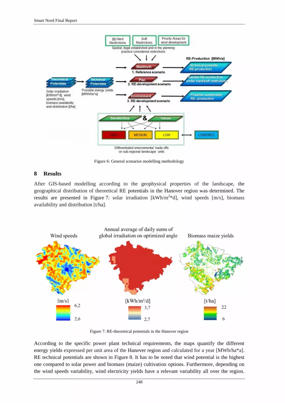
Smart Nord Final Report
248
Figure 6: General scenarios modelling methodology
8 Results
After GIS-based modelling according to the geophysical properties of the landscape, the
geographical distribution of theoretical RE potentials in the Hanover region was determined. The
results are presented in Figure 7: solar irradiation [kWh/m2*d], wind speeds [m/s], biomass
availability and distribution [t/ha].
Figure 7: RE-theoretical potentials in the Hanover region
According to the specific power plant technical requirements, the maps quantify the different
energy yields expressed per unit area of the Hanover region and calculated for a year [MWh/ha*a].
RE technical potentials are shown in Figure 8. It has to be noted that wind potential is the highest
one compared to solar power and biomass (maize) cultivation options. Furthermore, depending on
the wind speeds variability, wind electricity yields have a relevant variability all over the region.

SmartSpatial
249
However, the average solar electricity yields 420 MWh/ha*a on agricultural areas are similar to the
wind ones 441 MWh/ha*a.
Figure 8: RE technical potentials in the Hanover region
The average biomass electricity production is 27 MWh/ha*a. Furthermore, as heat production as an
important by-product of power production from biogas is a relevant component, we estimate the
heat yields for biomass (maize) cultivation, which vary from 20.7 to 77.3 MWh/ha*a with an
average heat production of 48 MWh/ha*a. As limitation for RE exploitation, we take into account
current restrictions for RE development which are either legally binding regulations such as laws,
defined as hard restriction areas, or from different recommendations by official planning
institutions, mentioned as soft restriction areas. The possible suitable areas are shown in Figure 9,
where the percentages displayed are referred to the whole regional area.
Figure 9: Hard and soft restriction areas, and suitable areas for each RE development,
calculated as a percentage of the whole regional area.

Smart Nord Final Report
250
In the Hanover region, hard restriction areas differ largely among the assessed possible exploitation
of wind power (59 %) on the one hand versus PV power plants (13 %) and energy maize
cultivation (23 %) on the other hand. The mapping of soft restriction areas for both, PV power
plants and maize cultivation, reveal more than the 50 % of the regions’ total area are considered
sensitive to development according to planning recommendations; while for wind only 28 % of the
total area are classified as sensitive areas. Regarding the remaining areas after subtraction of both
hard and soft restricted areas, wind energy exploitation is more limited with 14 %, followed by
maize cultivation with 27 % and PV power plants with 37 % share of the regions’ total area.
In order to take into account the sensitivity and values of relevant objects of environmental
protection, we produce separately sensitivity and values maps, which are then aggregated to
complete the spatial environmental analysis. As an example, we show here the aggregated and the
single environmental sensitivity and values maps for wind development. Taking into account as
relevant environmental objects flora, avifauna and human health, we estimated 56 % of the regions
area as highly sensitive and 37 % as medium sensitive, while 7 % were estimated to exhibit a low
sensitivity (Figure 10).
Figure 10: Wind power - map of sensitivity and value levels
of relevant objects of environmental protection
When additionally including areas with previous environmental impacts into the sensitivity
analyses (i.e. due to noise emissions from existing main roads), suitable areas for wind
development increase, as shown in Figure 11.

SmartSpatial
251
Figure 11: Wind power - map of lowered sensitivities due to previous environmental impacts.
Finally, energy scenarios are modelled taking into account the technical energy potentials and the
integration of spatial restrictions and environmental sensitivities and values. Figure 12 and Table 4
show the energy scenarios for wind-development and the combination of wind and solar power. By
developing energy scenarios, we estimate potentially producible energy yields under the different
RE-development scenarios conditions.
As final results of the Smart Nord sub-project six, Table 7 and Figure 12 illustrate the suitable areas
[ha] and possible electricity yields [GWh/a] for wind development according to the reference,
named as scenario “Maximum” and the two different RE-development scenarios, named as “Plan”
and as “Enviroment”. The model allows also calculating the predicted number of wind power
plants and, therefore, the installable power [GW].
Scenario
“Maximum”
Scenario “Plan” Scenario “Environment”
areas and potentials for wind electricity production
technical
requirements
hard
restrictions
soft
restrictions
low
sensitivities
medium
sensitivities
lowered
sensitivities
(previous
impacts)
Area [ha] 229,304 86,978 25,586 7,593 14,225 27,579
Proportion of Area [%] 100 38 11 3 6 12
Wind Power Stations [n] 25,992 10,905 3,520 1,110 2,085 3,774
Energy Yield [GWh/a] 11,473 4,959 1,850 552 1,077 1,780
Installable Power [GW] 79 33 11 3 6 12
Table 7: Wind power - total exploitable electricity yields and suitable areas according to different scenarios

Smart Nord Final Report
252
Figure 12: Possible sites for wind development by combining energy potentials
and environmental sensitivities and values
The possible wind energy yield according to the technical potential (scenario “Maximum”) is
estimated around 11,473 GWh/a on the regions total area. According to the scenario “Plan”, when
hard restriction areas are excluded, the potential is reduced to 4,959 GWh/a on 38 % of that area. If
all (hard and soft) restricted areas are excluded from the possible production area, 1,850 GWh/a
remain to be exploited on 11 % of the regions area. By contrast, the differentiated environmental
analysis assessed in the scenario “Environment” suggests that the low sensitivity areas amount to
853 GWh/a on 5 % of the technically exploitable area.
When considering lowered sensitivities due to previous environmental impacts, we estimated wind
energy yields of to 1,780 GWh/a on 12 % of the technically exploitable area.
Table 8 and Figure 13 finally show the combination of wind and biomass (maize) energy on
agricultural areas according to combined potentials and environmental analyses, with a total share
of 8 % of the total area. Taking into account that we assume a maize cultivation covers
approximately 20 % of the agricultural areas, the possible energy yields according to the technical
potentials and environmental sensitivity and values (scenario “Environment”) is estimated at
99 GWh/a on low sensitivity areas and at 1,139 GWh/a on medium sensitivity areas.
Scenario “Environment”
Areas and potentials for electricity
production Areas and potentials for heat production
areas of low
sensitivities
areas of
intermediate
sensitivities
areas of low
sensitivities
areas of
intermediate
sensitivities
Area [ha] 1,455 15,849 1,455 15,849
Proportion of
area [%] 1 7 1 7
Wind energy
yields [GWh/a] 83 912 - -
Biomass energy
yields [GWh/a] 6 81 10 146
Table 8: Wind and solar power - total exploitable electricity yields and
suitable areas according to different scenarios
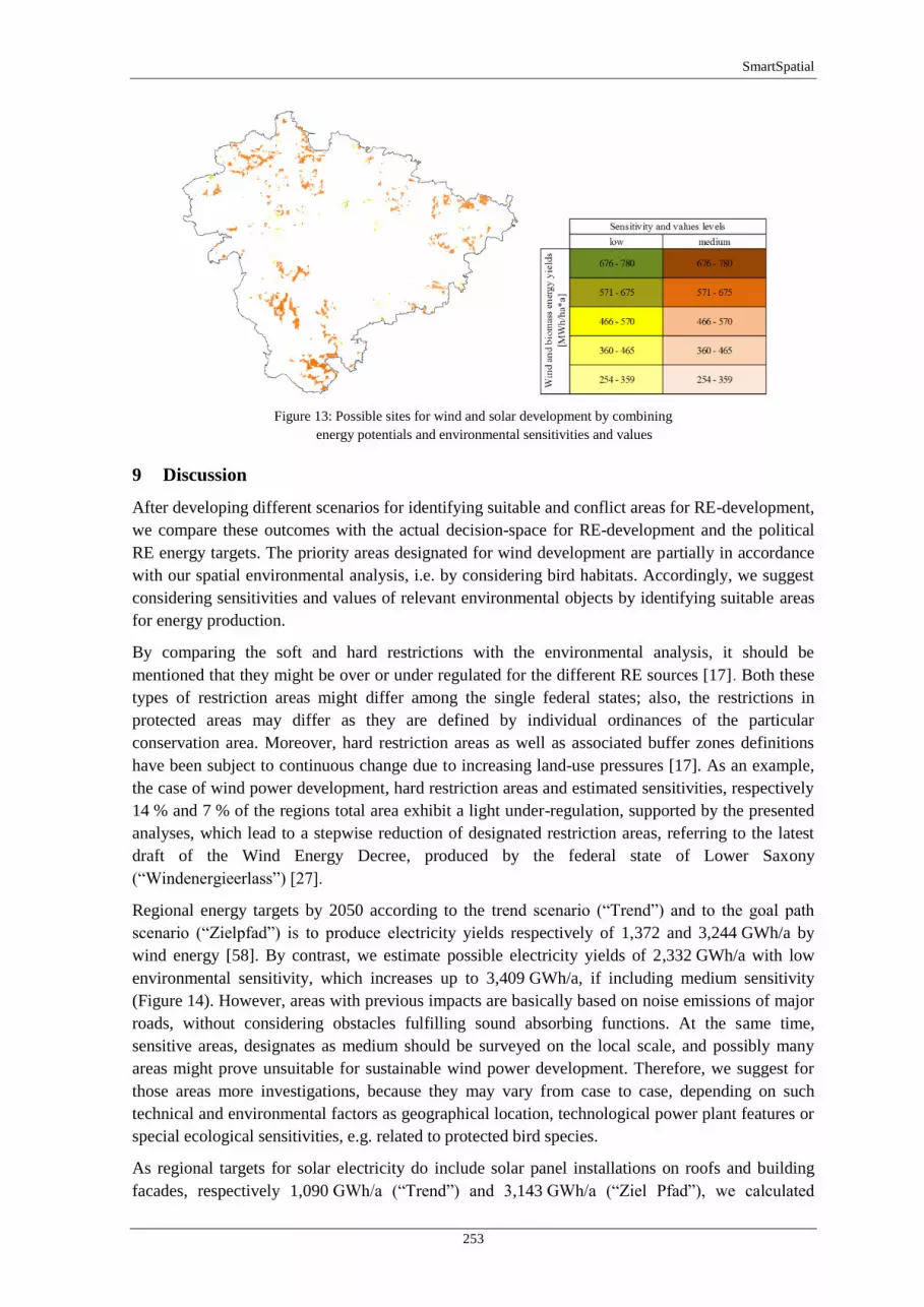
SmartSpatial
253
Figure 13: Possible sites for wind and solar development by combining
energy potentials and environmental sensitivities and values
9 Discussion
After developing different scenarios for identifying suitable and conflict areas for RE-development,
we compare these outcomes with the actual decision-space for RE-development and the political
RE energy targets. The priority areas designated for wind development are partially in accordance
with our spatial environmental analysis, i.e. by considering bird habitats. Accordingly, we suggest
considering sensitivities and values of relevant environmental objects by identifying suitable areas
for energy production.
By comparing the soft and hard restrictions with the environmental analysis, it should be
mentioned that they might be over or under regulated for the different RE sources [17]. Both these
types of restriction areas might differ among the single federal states; also, the restrictions in
protected areas may differ as they are defined by individual ordinances of the particular
conservation area. Moreover, hard restriction areas as well as associated buffer zones definitions
have been subject to continuous change due to increasing land-use pressures [17]. As an example,
the case of wind power development, hard restriction areas and estimated sensitivities, respectively
14 % and 7 % of the regions total area exhibit a light under-regulation, supported by the presented
analyses, which lead to a stepwise reduction of designated restriction areas, referring to the latest
draft of the Wind Energy Decree, produced by the federal state of Lower Saxony
(“Windenergieerlass”) [27].
Regional energy targets by 2050 according to the trend scenario (“Trend”) and to the goal path
scenario (“Zielpfad”) is to produce electricity yields respectively of 1,372 and 3,244 GWh/a by
wind energy [58]. By contrast, we estimate possible electricity yields of 2,332 GWh/a with low
environmental sensitivity, which increases up to 3,409 GWh/a, if including medium sensitivity
(Figure 14). However, areas with previous impacts are basically based on noise emissions of major
roads, without considering obstacles fulfilling sound absorbing functions. At the same time,
sensitive areas, designates as medium should be surveyed on the local scale, and possibly many
areas might prove unsuitable for sustainable wind power development. Therefore, we suggest for
those areas more investigations, because they may vary from case to case, depending on such
technical and environmental factors as geographical location, technological power plant features or
special ecological sensitivities, e.g. related to protected bird species.
As regional targets for solar electricity do include solar panel installations on roofs and building
facades, respectively 1,090 GWh/a (“Trend”) and 3,143 GWh/a (“Ziel Pfad”), we calculated

Smart Nord Final Report
254
additional possible electricity yields of 1,232 GWh/a on low sensitivity agricultural areas and of
13,931 GWh/a with the addition of the medium sensitivity areas produced by open-space solar
panels. However, the construction of open-solar panel on the surveyed agricultural land is currently
not politically promoted and, therefore, not supported by the incentive-based Renewable Energy
Act [59], [60], [61]. Finally, regional targets for biogas energy production do take into account also
wood and sewer gas for the heat component, while we consider maize only. Nevertheless, one
arable land will only be used for either maize production or for the production of other
energetically usable biomass. But, by the use of different bioenergy crops, negative impacts on the
environment can be reduced and more acreage could be used for energy production [62]. However,
by comparing the results and selecting the low sensitivity areas, we estimate for electricity
production around 232 GWh/a, which is near to 196 GWh/a (“Trend”), but far away to 323 GWh/a
(“Ziel Pfad”). On the other hand, heat production of biogas plants on low sensitivity areas accounts
417 GWh/a and 739 GWh/a compared to 462 (“Trend”) and 921 GWh/a (“Ziel Pfad”).
Figure 14: Comparison of regional energy targets by 2050 with environment-oriented scenarios
If the required spatial efficiency and the objectives of climate and environmental protection are to
be reached, it is necessary to combine spatial information on both, sectorial and combined RE
potentials as well as possible environmental impacts. This way, potential (co-)allocation options for
RE development can be analysed in order to maximize energy generation and at the same time
minimize environmental trade-offs [17], [20].
As showed for the here presented case study, the developed methodology is an important first step
in supporting regional decisions for the development and allocation of RE systems. Based on data
that are available for all German and most European regions, SmartSpatial can calculate the trade-
offs but also opportunities of regional RE-development at the beginning of the planning decision
process in a given region. The regional case study in the Hanover region with its high amount of
potentially conflicting land-use demands reveals that both, yields and environmental sensitivities
and values can vary widely with RE siting decisions. The differentiated environmental analysis in
combination with the spatially differentiated RE potential offers the best opportunities to find
optimized solutions which may also integrate political preferences or citizen opinions. If low
sensitive areas are not sufficient, medium sensitivity areas can be considered – given adequate
compensation of impaired ecosystem functions. This strategy offers the maximal energy yield with
a low consumption of land. Furthermore, areas that are already environmentally impacted, e.g. by
previously existing infrastructure projects are suitable, as long as they offer satisfactory energy
yields. In order to find these areas, the interplay between high potential energy yields and
environmental sensitivities should be analysed for each region individually. Of course, input data
are decisive for the results. On the one hand, technical wind energy potentials can be more
precisely estimated, if wind frequency distributions are available as well as the average wind
speeds at 100 m above the ground level. On the other hand, the evaluation of the visual landscape is

SmartSpatial
255
strong affected by the values of the Regional planning programme (RROP), in particular on
recreational areas. This evaluation had an almost prohibitive effect on the possibility to develop
additional RE in the region.
If other options have to be taken into account in order to reach RE production targets, which might
be less favourable regarding nature, we recommend considering possible mitigation measures in
order to use synergies (e.g. inclusion of previous environmental impacts into development
strategies) and therefore prevent invasive impacts. In fact, this general approach has already found
its way into planning, with the siting of wind power plants along infrastructure [43], as well as the
incentive-based steering by the EEG, with the siting of open-space solar panels exclusively up to
110 m along road infrastructure, on conversion areas from commercial or military utilization, or in
commercial and industrial areas69
[61]. One way to increase the decision space would be to use
more differentiated spatial analysis in order to achieve a high spatial efficiency. In this context,
spatial efficiency can be defined as appropriate site selection. To avoid possible land-use conflicts
and trade-offs between renewable energy production and nature conservation, regional land-use
planners need spatially explicit information in order to find the best development alternative.
Rather than undifferentiated restriction areas, RE development planning needs to be specific as to
which area specific pressures, sensitivities and values are of concern for the particular RE source
and their efficient combinations.
10 Conclusions and Recommendations
In SP 6 we develop the SmartSpatial model, which is based on a spatial multi-criteria
methodological framework for RE siting, following the objectives of sustainability by
simultaneously maximizing the spatial efficiency and minimizing the environmental impacts of RE
production. Thus, the model offers a great potential for the improvement of RE planning decisions.
Methodologically, the model combines RE-potential analysis with an ecological impact analysis,
which is specified for different RE pressure factors. The results obtained offer advanced insights on
regional RE development problems and chances. Furthermore, supporting a decentralised energy
production, spatial RE potentials can be used as an input to further develop electrical grid
infrastructures, in particular micro-grids (SP 1-5).
The spatially explicit approach and the opportunity to calculate RE production possibilities in
relation to environmental sensitivities and values, needs to integrate further considerations by
minimizing costs (SP 2). Further research development can include economic market constraints,
availability of transmission infrastructure, and current and future electricity loads (SP 1-4). The
interface between engineering and environmental planning, being currently underdeveloped, can
make a major contribution to transdisciplinary research on the one hand, and finding solutions for
major social problems on the other hand. Furthermore, the implementation of SmartSpatial at local
scale can be suggested for further research improvement. Accordingly, during Smart Nord, we
assess energy potentials from solar and geothermal sources for the municipality of Ganderkesee in
Lower Saxony, which will be compared in a next step to those estimated in the associated project
“EnerGeoPlan”. Also the regional energy potentials will be compared with the results at European
scale reached in SP 4.
Moreover, the biogas power plant allocation can be optimized by finding optimal site network
according to biomass potentials and environmental sensitivities and values and by minimizing
maize transportation and extraction costs (SP 5). This can have positive effects on the successful
achievement of regional RE production targets including optimized relations between spatial
69
cfr. §32 EEG.

Smart Nord Final Report
256
energy yields and environmental impacts, reducing planning uncertainties and the pitfalls of nature
conservation law as well as enhanced acceptance of future RE and electricity grid development.
These achievements are supported primarily by spatially explicit visualizations and calculations of
diverse RE development scenarios. In future research, economic and social considerations can be
integrated and optimized, for representation of a real level of renewable generation that may be
then deployed for allocating efficient energy combinations. Having provided basically preparatory
work for further optimization processes, we recommend further developing the presented spatial
multi-criteria model, which is an effective tool for RE-development, supporting regional and local
planning authorities to track changes and identify the best solutions.
References
[1] Bundesministerium für Umwelt, Naturschutz, Bau und Reaktorsischerheit (BMUB), “Erneuerbare
Energien. Innovationen für eine nachhaltige Energiezukunft,” October 2011.
[2] W. Brücher, “Energiegeographie,” in Energiegeographie-Wechselwirkungen zwischen Ressourcen,
Raum und Politik, Berlin, Stuttgart, Germany, Gebrüder Bornträger, 2009, ch. 1, pp. 1-280.
[3] J. Nitsch, W. Krewitt, M. Nast, P. Viebahn, S. Gärtner, M. Pehnt, et al., “Ökologisch optimierter
Ausbau der Nutzung erneuerbarer Energien in Deutschland,” March 2004.
[4] G. Reinhardt, K. Scheurlen, “Naturschutzaspekte bei der Nutzung erneuerbarer Energien,” June 2004.
[5] Bosch, Partner, “Vorbereitung und Begleitung der Erstellung des Erfahrungsberichtes 2007 gemäß
§20 EEG,” November 2007.
[6] Bosch, Partner, “Planerische Steuerung der Naturschutz Erneuerbarer Energien-Möglichkeiten und
Grenzen,” December 2010.
[7] M. Rodrigues, C. Montañés, N. Fueyo, “A method for the assessment of the visual impact caused by
the large-scale deployment of renewable-energy facilities,” in Environmental Impact Assessment
Review (Ed.) 30, 2010, 240-246.
[8] S. Bosch, G. Peyke, “Raum und Erneuerbare Energien. Anforderungen eines erneuerbaren
Energiesystems an die Standortplanung,” in Standort, vol.34, Springer-Verlag, Germany, 2010, pp.
11-19.
[9] T. Chang, E. Nielsen, W. Auberle, F. I. Solop, “A quantitative method to analyze the quality of EIA
information in wind energy development and avian/bat assessments,” in Environmental Impact
Assessment Review, 382013, 2013, pp. 142-150.
[10] C. V. Haaren, C. Palmas, T. Boll, M. Rode, M. Reich, F. Niederstadt, et al., “Erneuerbare Energien —
Zielkonflikte zwischen Natur- und Umweltschutz,” in BBN (Ed.), Neue Energien — Neue
Herausforderungen: Naturschutz in Zeiten der Energiewende, Jahrbuch Naturschutz und
Landschaftspflege, 59, 2013, pp. 18–33.
[11] M. Althaus, “Schnelle Energiewende — bedroht durch Wutbürger und Umweltverbände? Protest,
Beteiligung und politisches Risikopotenzial für Großprojekte im Kraftwerk- und Netzausbau,” in
Wissenschaftliche Beiträge, 15TH Wildau, 2012, pp. 103–113.
[12] S. Becker, L. Gailing, N. Naumann, “Neue Akteurslandschaften der Energiewende. Aktuelle
Entwicklungen in Brandenburg,” in Raumplanung162/3, 2012, pp. 42–46.
[13] P. Buschmann, “The German energy (half) turnaround, an analysis of soft-power mechanisms that
shape the German energy transformation,” Master Thesis, Series in environmental studies and
sustainable science, No. 2013 Lund University, 2013, p. 021.
[14] C. Kemfert, J. Horne, “Good governance of the Energiewende in Germany: wishful thinking or
manageable? Hertie school experts on the federal elections 2013,” July 2013.
[15] K. Calvert, J. M. Pearce, W. E. Mabee, “Toward renewable energy geo-information infrastructures:
applications of GIScience and remote sensing that build institutional capacity,” in Renewable and
sustainable energy reviews, vol. 18, 2013, pp. 416–429.
[16] W. Peters, “Erneuerbare Energien – Strategien für eine naturverträgliche Nutzung,” 2013.
[17] C. Palmas, A. Siewert, C. V. Haaren, “Exploring the decision-space for renewable energy generation
to enhance spatial efficiency,” in Environmental Impact Assessment Review (Ed.), 52, 2014, pp. 9–
17.

SmartSpatial
257
[18] C. Palmas, E. Abis, C. V. Haaren, A. Lovett, “Renewables in residential development: an integrated
GIS-based multicriteria approach for decentralized micro-renewable energy production in new
settlement development: a case study of the eastern metropolitan area of Cagliari, Sardinia, Italy,” in
Energy, Sustainability and Society 2012, 2, 2012, p. 10.
[19] H. Diefenbacher, “Zum Konfliktpotenzial Erneuerbarer Energien,” in soFid Sozialwissenschaftlicher
Fachinformationsdienst. International Beziehungen/Friedens- und Konflitkforschung, vol. 2009/2,
2009, pp. 9–18.
[20] C. V. Haaren, C. Palmas, A. Siewert, T. Boll, “Landschaft: Gesellschaftliche und wissenschaftliche
Herausforderungen der Energiewende,” in Eidg. Forschungsanstalt für Wald, Schnee und Landschaft
WSL (Hrsg.): Landschaft und Energiewende. Der Einfluss erneuerbarer Energien auf die Landschaft,
WSL Berichte 21 – Forum für Wissen, 2014, pp. 25-28.
[21] Region Hannover, “Landschaftsrahmenplan der Region Hannover,” 2013.
[22] Bundesamt für Naturschutz (BfN), May 2014.
[23] Landesamt für Statistik Niedersachsen (LSN), “Statistisches Taschenbuch 2014,” 2014.
[24] Region Hannover, “Regionalplanung in der Region Hannover,” 2014.
[25] J. X. Domínguez Bravo, I. García Casals, I. Pinedo Pascua, “J. X. Domínguez Bravo, I. García Casals,
I. Pinedo Pascua” in: Energy Policy, 35, 2007, pp. 4879–4892.
[26] LGLN Niedersachsen, “Auszug aus den Geobasisdaten der Niedersächsischen Vermessungs- und
Katasterverwaltung,” ATKIS Basis-DLM (2012) [ESRI ArcMap Digital Edition], 2012.
[27] Ministerium für Umwelt, Energie und Klimaschutz (MU), “Planung und Genehmigung von
Windenergieanlagen an Land in Niedersachsen und Hinweise für die Zielsetzung und Anwendung
(Windernergieerlass),” July 2012
[28] Niedersächsischen Landkreistag (NLT), “Naturschutz und Windenergie. Hinweise zur
Berücksichtigung des Naturschutzes und der Landschaftspflege bei Standortplanung und Zulassung
von Windenergieanlagen,” October 2014.
[29] Niedersächsischen Landkreistag (NLT), “Regionalplanung und Windenergie. Empfehlungen des NLT
zu den weichen Tabuzonen zur Steuerung der Windenergienutzung mit Ausschlusswirkung in
Regionalen Raumordnungsprogrammen,” February 2014.
[30] Ministerium für Umwelt, Energie und Klimaschutz (MU), “Verordnung über Schutzbestimmungen in
Wasserschutzgebieten” SchuVO, November 2009.
[31] J. Counihan, “Adiabatic atmospheric boundary layers: a review and analysis of data from the period
1880–1972,” in Atmos Environ, 79, 1975, pp. 871–905.
[32] J. S. Touma, “Dependence of the wind profile power law on stability for various locations,” in Air
Pollution Control Association, 27, 1977, pp. 863–866.
[33] EU Joint Research Centre (JRC), “model r.sun,” 2010.
[34] EU Joint Research Centre (JRC), “Clear sky indexes,” May 20014.
[35] S. Azam-Ali, N. M. J. Crout, R. G Bradley, “Perspectives in modelling resource capture by crops,”
Nottingham University Press, UK, 1994.
[36] R. Bauböck, “Optimizing Land use and the Yields of Bio-Energy Crops by using site specific
Biomass Calculations: Introduction of the Crop Modelling Software BioSTAR,” in R. Seppelt, A.A.
Voinov, S. Lange, D. Bankamp (Eds.), Managing Resources of a Limited Planet: Pathways and
Visions under Uncertainty, Sixth Biennial Meeting, Bankamp (Hrsg.), Leipzig, 2012, pp. 412–419.
[37] Bayerische Landesanstalt für Landwirtschaft (LfL), “Faustzahlen für die Biogaserzeugung,” 2008.
[38] J. Wiehe, M. Rode, H. Kanning, “Raumanalyse I – Auswirkungen auf Natur und Landschaft,” in M.
RODE AND H. KANNING (Eds) Natur- und raumverträglicher Ausbau energetischer
Biomassepfade, Stuttgart, ibidem-Verlag, 2010, pp. 21–90.
[39] W. Saathoff, C. Albert, C. V. Haaren, J. Hermes, M. Rode, F. Neuendorf, S. Hermann, “Optimierung
des Energiepflanzenbaus im Hinblick auf Natur und Landschaft,” in Abschlussbericht zum Projekt
Biomasse im Spannungsfeld. Unpublished.
[40] E. Smeets, R. Weterings, “Environmental Indicators: Typology and Overview,” Technical Report no.
5, EEA, Copenhagen, 1999, pp. 1-35.
[41] R. Bachfischer, “Die ökologische Risikoanalyse: eine Methode zur Integration natürlicher
Umweltfaktoren in die Raumplanung,” Ph.D. dissertation, Technische Universität München,
München, 1978, pp. 1-298.
[42] Region Hannover, “Regionales Raumordnungsprogramm 2005 für die Region Hannover,” 2005.

Smart Nord Final Report
258
[43] Bosch, Partner, “Abschätzung der Ausbaupotenziale der Windenergie an Infrastrukturachsen und
Entwicklung von Kriterien der Zulässigkeit,” in Final Report, Berlin, client: BMU,
Forschungszentrum Jülich PTJ, 2009, pp. 1-199.
[44] A. Garniel, U. Mierwald, “Vögel und Straßenverkehr,” Guideline, Michael-Otto-Institut, NABU,
Bonn, client: BMV, FE 02.286/2007/LRB, Bonn, 2010, pp. 1-133.
[45] H. Hötker, “Auswirkungen des Repowering von Windkraftanlagen auf Vögel und Fledermäuse,”
Final Report, Bergenhusen, client: Landesamt für Natur und Umwelt Schleswig Holstein, 2006, pp. 1-
40.
[46] Länderarbeitsgemeinschaft der Vogelschutzwarten (LAG-VSW), “Abstandsempfehlungen für
Windenergieanlagen zu avifaunistische bedeutenden Vogellebensräumen sowie Brutplätzen besonders
störungsempfindlicher oder durch Windenergieanlagen besonders gefährdeter Vogelarten,” May 2008.
[47] T. Dürr, “Vogelverluste an Windenergieanlagen in Deutschland, Daten aus der zentralen Fundkartei
der Staatlichen Vogelschutzwarte im Landesamt für Umwelt,” Gesundheit und Verbraucherschutz
Brandenburg, October 2013.
[48] R. Brinkmann, “Möglichkeiten und Grenzen der Integration tierökologischer Daten in die
Landschaftsplanung - dargestellt am Beispiel des Landschaftsplans Nenndorf,” in Inform. d.
Naturschutz Nieders., vol. 19, no. 2, 1999, pp. 90-104.
[49] Blasy, Overland, “Teilfortschreibung Konzentrationsflächen Windenergie. Ermittlung und Bewertung
der Konzentrationszonen,” August 2012.
[50] K. Runge, “Ökologische Auswirkungen von Freileitungen und Erdkabeln (380 kV),” April 2013.
[51] W. Nohl, “Landschaftsästhetische Auswirkungen von Windenergieanlagen,” September 2009.
[52] J. Peters et al., “Studie zur Bewertung der Wirkung von 380-kV-Freileitungen auf das
Landschaftsbild,” October 2008.
[53] Schallschutz im Städtebau, DIN 18005-1, 2002, July.
[54] Sechzehnte Verordnung zur Durchführung des Bundes-Immissionsschutzgesetzes (Sechzehnte
Verkehrslärmschutzverordnung – 16. BImSchV), 1990, June.
[55] Sechste Allgemeine Verwaltungsvorschrift zum Bundes-Immissionsschutzgesetz (Technisce
Anleitung zum Schutz gegen Lärm – TA Lärm), 1998, August.
[56] Niedersächsisches Gesetz über Verordnungen der Gemeinden zum Schutz vor Lärm
(Niedersächsisches Lärmschutzgesetz - NLärmSchG), 2012, December.
[57] F. Scholles, “Die ökologische Risikoanalyse und ihre Weiterentwicklung,” in D. Fürst and F.
Scholles, “Handbuch Theorien und Methoden der Raum- und Umweltplanung”, Rohn, Dortmund,
2008, ch. 7.6, pp. 458-479.
[58] Region Hannover, “Masterplan Stadt und Region Hannover. 100% für den Klimaschutz. Auf dem
Weg zu einer klimaneutralen Region bis 2050,” 2012.
[59] Gesetz für den Ausbau erneuerbarer Energien, Erneuerbare-Energien-Gesetz - EEG, 2014, July.
[60] S. Enkhardt, “Bundesregierung schränkt Flächen für Solarparks mit Ausschreibungen doch ein,”
February 2015.
[61] F. Staiß et al., “Nutzung der solaren Strahlungsenergie nach §11 EEG,” in Vorbereitung und
Begleitung der Erstellung des Erfahrungsberichtes 2007 gemäß §20 EEG, Report, ZSW, Stuttgart,
2007, ch. 8.9, pp. 68-77.
[62] M. Rode, H. Kanning, “Natur- und raumverträglicher Ausbau energetischer Biomassepfade,” Ibidem,
Stuttgart, 2010, pp. 1-156.


Annex
261
Annex


Annex
263
List of Publications Written in Smart Nord
M. Blank, S. Lehnhoff, “A Concept for Reliability Assessment for the Provision of Ancillary
Services,” in proc. of 2nd International Conference on Smart Grids and Green IT Systems
(Smart-Greens), May 9-10, 2013, Aachen, Germany.
C. Hinrichs, S. Lehnhoff, M. Sonnenschein, “A Decentralized Heuristic for Multiple-Choice
Combinatorial Optimization Problems,” in Operations Research Proceedings 2012 - Selected
Papers of the International Annual Conference of the German Operations Research Society
(GOR), Springer, pp. 297-302, 2014.
J. Bremer, M. Sonnenschein, “A Distributed Greedy Algorithm for Constraint-based
Scheduling of Energy Resources,” in 1st International Workshop on Smart Energy Networks &
Multi-Agent Systems, FedCSIS Proceeding, pp. 1285-1292, 2012.
S. Beer, “A Formal Model for Agent-based Coalition Formation in Electricity Markets,” in 4th
IEEE/PES Innovative Smart Grid Technologies Europe (ISGT EUROPE), Kopenhagen, pp. 1-
5, 2013.
M. Blank et al., “Agentenbasierte Vorhaltung und Erbringung von Primärregelleistung,” in at –
Automatisierungstechnik, Band 62, Heft 5, pp. 347-363, April 2014.
F. Fuchs, D. V. Pham, A. Mertens, “Analysis of grid current control in consideration of voltage
feedforward and cable capacitance demonstrated on a fully sized wind turbine installed in a
wind park,” Energy Conversion Congress and Exposition (ECCE), 2013 IEEE, pp.3325,3332,
15-19 Sept. 2013.
M. Blank, S. Lehnhoff, “Assessing Reliability of Distributed Units with Respect to the
Provision of Ancillary Services,” in proc. of 11th IEEE Conference on Industrial Informatics
(INDIN), Special Session on Industrial Informatics in Smart Grids, Bochum, Juli 2013.
J. Bremer, M. Sonnenschein, “Automatic Reconstruction of Performance Indicators from
Support Vector based Search Space Models in Distributed Real Power Planning Scenarios,” in
Proceedings of the Informatik 2013 - Informatik angepasst an Mensch, Organisation und
Umwelt, Koblenz, Germany. LNI 220, pp. 1441-1454, 2013.
R. Bleiker, S. Lehnhoff, C. Mayer, K. Piech, “Automatisierung heterogener, verteilter
Energieanlagen mittels OPC UA,” in Zukünftige Stromnetze für Erneuerbare Energien, Berlin,
Germany, 2014.
F. Fuchs, R. Dietz, S. Garske, T. Breithaupt, A. Mertens, L. Hofmann, “Challenges of Grid
Integration of Distributed Generation in the Interdisciplinary Research Project Smart Nord,”
IEEE 5th International Symposium on Power Electronics for Distributed Generation Systems
(PEDG), Galway, Ireland, 24.-27. June 2014.
J. Psola et al., “Characteristics of Energy Storage in Smart Grids,” EVER2014, Monaco,
Monaco, 2014.
C. Hinrichs, S. Lehnhoff, M. Sonnenschein, “COHDA: A Combinatorial Optimization
Heuristic for Distributed Agents,” in Agents and Artificial Intelligence, Communications in
Computer and Information Science, Vol. 449, Springer, pp. 23-29, 2014.
A. Nieße, S. Beer, J. Bremer, C. Hinrichs, O. Lünsdorf, M. Sonnenschein, “Conjoint Dynamic
Aggregation and Scheduling Methods for Dynamic Virtual Power Plants,” in Proceedings of

Smart Nord Final Report
264
the 2014 Federated Conference on Computer Science and Information Systems, pp. 1505-1514,
2014.
M. Blank, S. Lehnhoff, “Considering Correlations for Reliable Distributed Ancillary Service
Provision,” in proc. of 5th IEEE PES Innovative Smart Grid Technologies (ISGT) Europe,
October 12-14, 2014, Istanbul, Turkey.
J. Bremer, M. Sonnenschein, “Constraint-Handling for Optimization with Support Vector
Surrogate Models: A Novel Decoder Approach,” in Proceedings of the 5th International
Conference on Agents and Artificial Intelligence, Volume 2, Barcelona, Spain, 15-18 February.
SciTePress, pp. 91-105, 2013.
J. Bremer, M. Sonnenschein, “Constraint-Handling with Support Vector Decoders,” in Agents
and Artificial Intelligence, Communications in Computer and Information Science, Vol. 449,
Springer, pp. 228-244, 2014.
M. Blank, S. Lehnhoff, “Correlations in Reliability Assessment of Agent-based Ancillary-
Service Coalitions,” in proc. of 18th Power Systems Computation Conference (PSCC), August
18-22, 2014, Wroclaw, Poland.
M. Sonnenschein, O. Lünsdorf, J. Bremer, M. Tröschel, “Decentralized control of units in
smart grids for the support of renewable energy supply”, Environmental Impact Assessment
Review (in press).
C. Köpp, H.-J. von Mettenheim, M. H. Breitner, “Decision Analytics mit Heatmap-
Visualisierung von mehrschrittigen Ensembledaten,” Wirtschaftsinformatik: 147.
doi:10.1007/s11576-014-0417-3.
A. Nieße, M. Tröschel, M. Sonnenschein, “Designing Dependable and Sustainable Smart Grids
- How to Apply Algorithm Engineering to Distributed Control in Power Systems,”
Environmental Modelling and Software, Vol. 56, pp. 37-51, 2014.
M. Sonnenschein, H.-J. Appelrath, L. Hofmann, M. Kurrat, S. Lehnhoff, C. Mayer,
A. Mertens, M. Uslar, A. Nieße, M. Tröschel, “Dezentrale und selbstorganisierte Koordination
in Smart Grids,” VDE-Kongress 2012 - Intelligente Energieversorgung der Zukunft, Stuttgart,
2012.
S. Lehnhoff et al., “Distributed Coalitions for Reliable and Stable Provision of Frequency
Response Reserve – An Agent-based Approach for Smart Distribution Grids,” in proc. of IEEE
International Workshop on Intelligent Energy Systems (IWIES), IEEE Press, 2013.
C. Hinrichs, J. Bremer, M. Sonnenschein, “Distributed Hybrid Constraint Handling in Large
Scale Virtual Power Plants,” in IEEE PES Conference on Innovative Smart Grid Technologies
Europe (ISGT Europe 2013), Kopenhagen, IEEE Power & Energy Society, 2013.
F. Fuchs, A. Mertens, “Dynamic modelling of a 2 MW DFIG wind turbine for converter issues:
Part 1,” Power Electronics and Motion Control Conference (EPE/PEMC), 2012 15th
International, pp.DS2d.5-1,DS2d.5-7, 4-6 Sept. 2012.
A. Nieße, S. Lehnhoff, M. Sonnenschein, M. Tröschel, “Dynamic Virtual Power Plants in
Future Energy Grids: Defining the Gap to the Field,” in VDE Kongress 2014, VDE Verlag,
2014.
F. Muuß, N. G. A. Hemdan, M. Kurrat, D. Unger, B. Engel, “Dynamic Virtual Reactive Power
Plant in Active Distribution Networks” – Powertec, Eindhoven 2015.

Annex
265
A. Ohsenbrügge et al., “Efficient Provision of Ancillary Services by Decentralized, Volatile
Generating Units,” to appear in proc. of VDE/ETG Fachtagung Von Smart Grids zu Smart
Markets, 25.-26. March 2015, Kassel, Germany.
F. Fuchs, D. V. Pham, A. Mertens, “Einfluss der Netzimpedanz auf die Dynamik der
netzseitigen Stromregelung am Beispiel einer Windenergieanlage,” ETG Kongress, Berlin,
2013.
S. C. Meyer, M. H. Breitner, “Electricity Associations as Marked - Based Steering Mechanism
and Alternative to Fixed Feed - in Tariffs,” Proceedings of the 28th EnviroInfo 2014
Conference: 729–734.
J. Bremer, M. Sonnenschein, “Estimating Shapley Values for Fair Profit Distribution in Power
Planning Smart Grid Coalitions,” in Multiagent System Technologies - Proceedings of the
MATES 2013, Koblenz, Germany. Springer, LNCS 8076, 2013.
C. Hinrichs, M. Sonnenschein, “Evaluation Guidelines for Asynchronous Distributed
Heuristics in Smart Grid Applications,” in Proceedings of the 28th Conference on
Environmental Informatics - EnviroInfo 2014 - ICT for Energy Efficiency, BIS-Verlag, pp. 365
– 372, 2014.
C. Hinrichs, M. Sonnenschein, S. Lehnhoff, “Evaluation of a Self-Organizing Heuristic for
Interdependent Distributed Search Spaces,” in ICAART 2013 - Proceedings of the 5th
International Conference on Agents and Artificial Intelligence, Volume 1 - Agents, Barcelona,
Spain, 15-18 February. SciTePress, pp. 25-34, 2013
G. Lohmann, M. R. R. Tabar, P. Milan, M. Anvari, M. Wächter, E. Lorenz, D. Heinemann,
J. Peinke, “Flickering Events in Wind and Solar Power,” in Proceedings of the 28th
International Conference on Informatics for Environmental Protection, Oldenburg, 2014, S.
723–728.
G Lohmann, J. Kühnert, E. Lorenz, A. Hammer, D. Heinemann, “Fluctuations in Large-Scale
Photovoltaic and Wind Power Feed-In,” in Proceedings of the 4th International Workshop on
Integration of Solar Power into Power Systems, Berlin, Germany, 2014.
S. Lehnhoff, M. Sonnenschein, M. Tröschel, “Forschungsverbund Smart Nord - Dezentrale und
selbstorganisierte Koordinationsverfahren für einen sicheren und zuverlässigen Netzbetrieb,” in
Konferenz für Nachhaltige Energieversorgung und Integration von Speichern - NEIS 2013 –
Tagungsband, S. 7-12, 2013.
C. Norrenbrock, O. Melchert, A. K. Hartmann, “Fragmentation properties of two-dimensional
Proximity Graphs considering random failures and targeted attacks,” (in Vorbereitung).
H.-J. Appelrath, G. Brunekreeft, A. Weidlich, C. Wissing, C. Mayer, A. Ohsenbrügge,
S.-C. Schnabel, M. Tröschel, “Future Energy Markets - Mehr Markt für eine effiziente
Energiewende,” acatech Materialien, 2014.
C. Rosinger, S. Beer, “Glaubwürdigkeit in dynamischen Wirkleistungsverbünden,” DACH-
Energieinformatik 2014, Zürich, 2014.
C. Rosinger, S. Beer, “Glaubwürdigkeit in dynamischen Wirkleistungsverbünden,” in
Informatik-Spektrum, pp. 1–8, Dezember 2014.
M. Calabria, W. Schumacher, “Impact of inverter clustering on the small-signal stability of a
grid,” in EnviroInfo, 2013.

Smart Nord Final Report
266
T. Breithaupt, T. Rendel, L. Hofmann, “INES - Integrierte Netz- und Energiemarktsimulation,”
15. Dresdener Kreis 2014, Fachtagung der TU-Dresden, der Universität Hannover, der
Universität Magdeburg und der Gesamthochschule Duisburg: Elektroenergieversorgung,
Leipzig, Deutschland, 19.-20. März 2014.
C. Rosinger, M. Uslar, J. Sauer, “Informationssicherheit als Vertrauenswürdigkeitsfacette für
selbstorganisierende Energieagenten,” in VDE-Kongress 2014, VDE Verlag, 2014.
Y. Chen, R. Hesse, D. Turschner, H. P. Beck, “Investigation of the Virtual Synchronous
Machine in the Island Mode,” 3rd IEEE PES Innovative Smart Grid Tech-nologies Europe
(ISGT Europe), Berlin, 2012.
M. R. R. Tabar, M. Anvari, G. Lohmann, D. Heinemann, M. Wächter, P. Milan, E. Lorenz,
J. Peinke, “Kolmogorov spectrum of renewable wind and solar power fluctuations,” European
Physical Journal Special Topics, Bd. 223, Nr. 9, S. 1–8, Juli 2014.
J. Bremer, M. Sonnenschein, “Kommunikation von Umweltkennzahlen im Smart Grid und
deren Integration in die verteilte Wirkleistungsplanung,” in IT-gestütztes Ressourcen- und
Energiemanagement, Konferenzband zu den 5. BUIS-Tagen, Oldenburg, Springer, S. 35-47,
2013.
T. Dewenter, A. K. Hartmann, “Large-deviation properties of power grids,” Münster, 6. März
2014, "Complexity Meets Energy" workshop.
T. Dewenter, A. K. Hartmann, “Large-deviation properties of power grids,” Dresden, 4. April
2014, DPG Frühjahrstagung.
T. Dewenter, A. K. Hartmann, “Large-deviation properties of resilience of power grids,” New
J. Phys. 17, 015005 (2015).
T. Dewenter, A. K. Hartmann, “Large-deviation properties of resilience of power grids,” Bad
Honnef, 6.-9. Dezember 2014, “HEEECC - Health, Energy & Extreme Events in a Changing
Climate”, 577. WE-Heraeus-Seminar.
A. K. Hartmann, “Large-deviation properties of resilience of transportation networks,” Eur.
Phys. J B 87, 114 (2014).
A. K. Hartmann, “Large-deviation properties of simple energy-grid models,” Regensburg, 12.
März 2013, DPG Frühjahrstagung.
A. K. Hartmann, T. Dewenter, W. Heins, B. Werther, “Large-deviation study of the maximum-
disturbance stability of power grids,” 19. März 2014, DPG Frühjahrstagung, Berlin.
C. Köpp, H. J. von Mettenheim, M. H. Breitner, “Lastmanagement in Stromnetzen - Beiträge
für ein Entscheidungsunterstützungssytem für Portfoliobetreiber,” Wirtschaftsinformatik: 1–11.
doi:10.1007/s11576-012-0348-9.
C. Wissing, A. Nieße, M. Tröschel, “Market-Based redispatch in distribution Grids,”
IRES, 2013.
S. Lehnhoff, M. Tröschel, M. Uslar, C. Wissing, H.-J. Appelrath, M. Sonnenschein, “Market-
based self-organized provision of active power and ancillary services: An agent-based
approach for Smart Distribution Grids,” in Complexity in Engineering (COMPENG), pp. 1-5,
2012.

Annex
267
T. Breithaupt, S. Garske, T. Rendel, L. Hofmann, “Methodological Approach for Integrated
Grid and Market Simulation of Coherent Distribution and Transmission Systems,” EnviroInfo
2013, Hamburg, Germany, 02.-04. September 2013.
J. Bremer, M. Sonnenschein, “Model-based Integration of Constrained Search Spaces into
Distributed Planning of Active Power Provision,” in Computer Science and Information
Systems, Vol. 10, No. 4, 1823-1854, 2013.
J. Psola, et al., “Modeling of a Redox Flow Battery Storage for Grid Applications,” in
PCIMasia 2013, Shanghai, China, 2013.
M. Calabria, W. Schumacher, “Modeling power inverter interactions in a low voltage grid,” in
s Control and Modeling for Power Electronics (COMPEL), 2014 IEEE 15th Workshop on,
2014.
T. Breithaupt, T. Rendel, C. Rathke, L. Hofmann, “Modeling the Reliability of Large Thermal
Power Plants in an Integrated Grid and Market Model,” 2012 IEEE International Conference
on Power System Technology (Powercon), Auckland, New Zealand, 30. October–2. November
2012.
Y. Chen, B. Werther, B. Schwake, H.-P. Beck, “Netzstabilisierung durch die "Virtuelle
Synchronmaschine" (VISMA) mit überlagerter Frequenz- und Spannungsregelung,”
Internationaler ETG-Kongress 2013, Berlin (05.-06. November 2013).
G. Anders, C. Hinrichs, F. Siefert, P. Behrmann, W. Reif, M. Sonnenschein, “On the Influence
of Inter-Agent Variation on Multi-Agent Algorithms Solving a Dynamic Task Allocation
Problem under Uncertainty,” in 2012 IEEE Sixth International Conference on Self-Adaptive
and Self-Organizing Systems (SASO 2012), Lyon, France, 2012.
T. Dewenter, B. Werther, A. K Hartmann, H.-P. Beck, “Optimierung des dynamischen
Verhaltens netzstützender Anlagen am Beispiel der Virtuellen Synchronmaschine,” 13.
Symposium Energieinnovation, Graz/Austria, (12.-14. Februar 2014).
J. Psola et al., “Optimization of energy output by combining energy storages with renewable
energies,” in PCIMasia 2014, Shanghai, China, 2014.
J. Bremer, M. Sonnenschein, “Parallel tempering for constrained many criteria optimization in
dynamic virtual power plants,” in 2014 IEEE Symposium on Computational Intelligence
Applications in Smart Grids (CIASG), IEEE, 2014.
C. Norrenbrock, “Percolation threshold on planar Euclidean Gabriel graphs,” arXiv:1406.0663.
F. Fuchs, M. Mertens, “Prediction and avoidance of grid-connected converter's instability
caused by wind park typical, load-varying grid resonance,” Energy Conversion Congress and
Exposition (ECCE), 2014 IEEE, pp.2633,2640, 14-18 Sept. 2014.
Y. Chen, R. Hesse, D. Turschner, H.-P. Beck, “Propiedades dinamicas da maquina sincrona
virtual,” EM Janeiro 2014, S. 58 - 65, (2014).
N. G. A. Hemdan, F. Muuß, D. Unger, M. Kurrat, “Reactive Power as an Ancillary Service
Provision into Transmission Networks through Decentralized Generation” in Cigre Belgium
2014.
M. Gandor et al., “Reconfiguration Strategies for Electrical Devices for Operation within
Feasibility Margins,” in proc. of VDE Kongress 2012 – Smart Grid Applications /
Services, 2012, Stuttgart, Germany.

Smart Nord Final Report
268
C. Wissing, H.-J. Appelrath, “ReFlex: Market-Based Redispatch in Distribution Grids -
Incentivizing Flexible Behavior of Distributed Energy Resources,” EnviroInfo. Hamburg,
September 2013.
M. R. R. Tabar, M. Anvari, M. Wächter, P. Milan, G. Lohmann, E. Lorenz, D. Heinemann,
J. Peinke, “Renewable Power from Wind and Solar: Suppressing The Short-Term Intermittency
and Their Resilience,” (submitted).
C. Rosinger, M. Uslar, F. Hockmann, “Reputationssysteme für selbstorganisierte Multi-
Agenten-Systeme in Energiemanagementsystemen,” VDE-Kongress 2012, 2012.
M. R. R. Tabar, M. Anvari, M. Waechter, P. Milan, G. Lohmann, E. Lorenz, D. Heinemann,
J. Peinke, “Resilience of Renewable Power from Wind and Solar and Suppressing Their Short-
Term Intermittency,” (Submitted).
J. Bremer, M. Sonnenschein, “Sampling the Search Space of Energy Resources for Self-
organized, Agent-based Planning of Active Power Provision,” in Environmental Informatics
and Renewable Energies - 27th International Conference on Informatics for Environmental
Protection. Shaker Verlag, pp. 214-222, 2013.
M. Sonnenschein, “Smart Grids - auf dem Weg zu intelligenten Stromnetzen,” in
Zukunftswerkstatt Deutschland: Die Energiewende. Vol. 8 Hanse Studien, S. 93-104, 2013.
M. Sonnenschein, M. Tröschel, O. Lünsdorf, “Smart Grids for Optimised Utilisation of
Renewable Energy Supply,” in Environmental Informatics and Renewable Energies - 27th
International Conference on Informatics for Environmental Protection. Shaker Verlag, pp. 178-
187, 2013.
M. Calabria, W. Schumacher, “Stability optimization for distributed generation of load-
following energy,” in Energy Conference (ENERGYCON), 2014 IEEE International, 2014.
M. Sonnenschein, C. Hinrichs, A. Nieße, U. Vogel, “Supporting Renewable Power Supply
through Distributed Coordination of Energy Resources,” in ICT Innovations for Sustainability,
Advances in Intelligent Systems and Computing. Springer, pp. 387-404, 2015.
M. Kurrat, N. G. A. Hemdan, B. Engel, R. Canders, M. Henke, “Technical challenges for
ancillary services provided by decentralized power generation in active distribution systems,”
in ETG Kongress Berlin 2013.
J. Psola, et al., “Technologies and Operational Concepts for Energy Storages,” in Enviroinfo,
Hamburg, Germany, 2013.
C. Hinrichs, M. Sonnenschein, “The Effects of Variation on Solving a Combinatorial
Optimization Problem in Collaborative Multi-Agent Systems,” in Multiagent System
Technologies. Lecture Notes in Computer Science Volume 8732, pp. 170-187, 2014.
C. Rosinger, M. Uslar, J. Sauer, “Threat Scenarios to evaluate Trustworthiness of Multi-agents
in the Energy Data Management,” in Environmental Informatics and Renewable Energies -
27th International Conference on Informatics for Environmental Protection. Shaker Verlag,
2013.
B. Küster, A. Koukal, M. H. Breitner, “Towards an Allocation of Revenues in Virtual Clusters
within Smart Grids,” IWI Diskussionbeiträge 60 (September), 2013.
Annex
269
S. Beer, M. Sonnenschein, H.-J. Appelrath, “Towards a Self-Organization Mechanism for
Agent Associations in Electricity Spot Markets,” in INFORMATIK 2011 – Informatik schafft
Communities., Berlin, 2011.
S. Lehnhoff, K. Piech, S. Rohjans, “UML-based Modeling of OPC UA Address Spaces for
Power Systems,” in IEEE International Workshop on Intelligent Energy Systems (IWIES
2013), Vienna, Austria, 2013.
C. Wissing, H.-J. Appelrath, “Using automated market analysis for optimized economic
operation of DER in Virtual Power Plants,” EEM, 2012.
A. Nieße, M. Sonnenschein, “Using Grid Related Cluster Schedule Resemblance for Energy
Rescheduling,” in SmartGreens 2013 - 2nd Int. Conf. on Smart Grids and Green IT Systems,
Aachen, Germany, pp. 22-31, 2013.
C. Rosinger, M. Uslar, J. Sauer, “Using Information Security as a Facet of Trustworthiness for
Self-Organizing Agents in Energy Coalition Formation Processes,” in Proceedings of the 28th
Conference on Environmental Informatics - EnviroInfo 2014 - ICT for Energy Efficiency, BIS-
Verlag, 2014.


Annex
271
List of Doctoral Theses
Almut Siewert, “Kumulative Wirkung von EE-Anlagen,” Leibniz Universität Hannover,
Institute of Environmental Planning, planned to be submitted 2016.
Anja Ohsenbrügge, “Entwicklung eines flexiblen Prognosemodells zur dynamischen
Regelleistungsbemessung,” University of Oldenburg, Department of Computing Science,
planned to be submitted 2015.
Astrid Nieße, “Verteilte kontinuierliche Einsatzplanung in Dynamischen Virtuellen
Kraftwerken,” University of Oldenburg, Department of Computing Science, 2015.
Carsten Wissing, “ReFlex: Marktbasiertes Redispatch mit Flexibilitäten von Netznutzern für
das Verteilnetz,” University of Oldenburg, Department of Computing Science, 2015.
Christian Hinrichs, “Selbstorganisierte Einsatzplanung dezentraler Akteure in Smart Grids,”
University of Oldenburg, Department of Computing Science, 2014.
Christine Rosinger, “Ein Vertrauensmodell für die Verbundbildung von Multi-Agenten-
Systemen im Energiedatenmanagement,” University of Oldenburg, Department of Computing
Science, planned to be submitted 2016.
Felix Fuchs, “Einfluss von Resonanzen der Netzimpedanz auf die Stromregelung von
Windenergieanlagen,” Leibniz Universität Hannover, Institut für Antriebssysteme und
Leistungselektronik, planned to be submitted 2015.
Fridolin Muuß, “Blindleistungsregelstrategien - intelligentes Blindleistungsmanagement durch
dezentrale Energieanlagen im aktiven Verteilnetz,” Technische Universität Braunschweig,
elenia, planned to be submitted 2017.
Gerald Lohmann, “Kleinskalige stochastische Simulation von Fluktuationen in der
Leistungsabgabe dezentraler Photovoltaikanlagen auf Verteilnetzebene,” University of
Oldenburg, Institute of Physics and ForWind, 2016.
Jan-Hendrik Psola, “Betriebs- und Einsatzmöglichkeiten von Energiepseichern,” Technische
Universität Braunschweig, Institute for Electrical Machines, Traction and Drives, planned to be
submitted 2015.
Jörg Bremer, “Constraint-Handling mit Supportvektor-Dekodern in der verteilten
Optimierung,” University of Oldenburg, Department of Computing Science, 2015.
Marita Blank, “Reliability Assessment of Coalitions for the Provision of Ancillary Services,”
University of Oldenburg, Department of Computing Science, planned to be submitted 2015.
Phillip Gronstedt, “Systembasierte Integration erneuerbarer Energieumwandlung über die
Mehrwegevermarktung virtueller Pools,” Technische Universität Braunschweig, 2013.
René Dietz, “Wechselwirkungen dezentraler Energieerzeuger kleiner Leistung im
Niederspannungsnetz,” Leibniz Universität Hannover, Institut für Antriebssysteme und
Leistungselektronik, planned to be submitted 2016.
Sebastian Beer, “Dynamic Coalition Formation in Electricity Markets,” University of
Oldenburg, Department of Computing Science, planned to be submitted 2015.


Closing Remarks
273
Closing Remarks
Looking back on the past three years, it can be claimed that the planned aims of Smart Nord were
achieved. It should especially be mentioned that due to the large number of participants numerous
collaborations between the young scientists resulted at the different research institutes which will
hopefully be continued after the end of Smart Nord.
The grant ended with the end of February 2015 where results of Smart Nord were presented to a
broad audience of interested visitors at the Smart Nord final conference. At this point, we would
like to thank again the organization committee and all speakers and supporters of the conference as
well as the contributors of this final report. In addition Dr. Martin Troeschel and Torsten Rendel
had to be thanked for their coordination of the project and support of the project management.
Smart Nord’s results are currently worked on in the transfer project “iQ –Intelligent Reactive
Power Control for Distribution Grids” which is funded by the Lower Saxony Ministry of Science.
Also the EXIST transfer project “Dynamic VPP” which revisits topics of Smart Nord must be
mentioned here. In addition to these projects directly linked to Smart Nord, two project funded by
the federal ministries of BMU and BMWI, one funded by the EU and five federal funded projects
are applied for. At last it must be mentioned that one partner is aiming to implement a DFG-
Forschergruppe.
A list of publications and adjacent doctoral theses can be found in the annex. For further
information do not hesitate to contact the authors of this final report.
We would like to express our gratitude to the Lower Saxony Ministry of Science for supporting
Smart Nord through the “Niedersächsisches Vorab” grant programme.
Prof. Dr.-Ing. habil. Lutz Hofmann Prof. Dr. rer. nat. habil. Michael Sonnenschein
Institute of Electric Power Systems Department of Computing Science
Leibniz Universität Hannover Carl von Ossietzky Universität Oldenburg


ISBN: 978-3-00-048757-6


