Oxygen Exosphere of Mars: Evidence from Pickup Ions

Oxygen Exosphere of Mars:

Evidence from Pickup Ions Measured by MAVEN

By

Ali Rahmati

Submitted to the graduate degree program in the Department of Physics and Astronomy,

and the Graduate Faculty of the University of Kansas in partial fulfillment of the

requirements for the degree of Doctor of Philosophy.

________________________________

Professor Thomas E. Cravens, Chair

________________________________

Professor Philip S. Baringer

________________________________

Professor David Braaten

________________________________

Professor Mikhail V. Medvedev

________________________________

Professor Stephen J. Sanders

Date Defended: 22 January 2016

ii

The Dissertation Committee for Ali Rahmati

certifies that this is the approved version of the following dissertation:

Oxygen Exosphere of Mars:

Evidence from Pickup Ions Measured by MAVEN

________________________________

Professor Thomas E. Cravens, Chair

Date approved: 22 January 2016

iii

Abstract

Mars possesses a hot oxygen exosphere that extends out to several Martian radii. The main

source for populating this extended exosphere is the dissociative recombination of molecular

oxygen ions with electrons in the Mars ionosphere. The dissociative recombination reaction creates

two hot oxygen atoms that can gain energies above the escape energy at Mars and escape from the

planet. Oxygen loss through this photochemical reaction is thought to be one of the main

mechanisms of atmosphere escape at Mars, leading to the disappearance of water on the surface.

In this work the hot oxygen exosphere of Mars is modeled using a two-stream/Liouville

approach as well as a Monte-Carlo simulation. The modeled exosphere is used in a pickup ion

simulation to predict the flux of energetic oxygen pickup ions at Mars. The pickup ions are created

via ionization of neutral exospheric oxygen atoms through photo-ionization, charge exchange with

solar wind protons, and electron impact ionization. Once ionized, the pickup ions are accelerated

by the solar wind motional electric field to high energies, thus detectable by spacecraft instruments.

The MAVEN (Mars Atmosphere and Volatile EvolutioN) spacecraft arrived at Mars in

September of 2014 and has been taking measurements in the upper atmosphere of Mars, with the

goal of determining the drivers and rates of atmospheric escape. In this work comparisons are

made between the pickup ion model results and the MAVEN data from the SEP (Solar Energetic

Particle) and SWIA (Solar Wind Ion Analyzer) instruments. It is shown that these model-data

comparisons can be used to constrain the hot oxygen exospheric densities and the associated

escape rates of oxygen from Mars.

iv

Acknowledgments

I would like to thank my advisor and dissertation committee chair, Professor Thomas Cravens, for his

invaluable support and excellent guidance. He made this research a very enjoyable experience for me, and

I learned a lot from him. I also wish to thank Professors Philip Baringer, David Braaten, Mikhail Medvedev,

and Stephen Sanders for serving on my dissertation committee. Many thanks also go to the KU Department

of Physics and Astronomy staff, Tizby Hunt Ward, Bob Curry, Teri Leahy, Kristin Rennells, Kim Hubbel,

Desiree Neyens, and Doug Fay, for patiently taking care of my paperwork. I had the joy of taking courses

with almost every professor in the physics department, and I’d like to thank them all for being such great

teachers.

This work would have not been accomplished without the remarkable effort by the entire MAVEN

team. For this project I’ve had very informative discussions with Steve Ledvina, Davin Larson, Rob Lillis,

Patrick Dunn, Jasper Halekas, Jane Fox, Andy Nagy, Stephen Bougher, Guillaume Gronoff, Matt Richard,

Johnathan Croxell, Ed Thiemann, Harsha Pothapragada, and Shotaro Sakai, and I thank them all. This work

was supported by NASA grant NNH10CC04C to the University of Colorado and by subcontract to the

University of Kansas. The MAVEN project is supported by NASA through the Mars Exploration Program.

During the five years of my PhD studies in Lawrence, Kansas, I’ve had the pleasure of being around

so many kind families and good friends. I would like to thank them all for making Kansas feel like home.

I especially thank Tom Cravens and Jean Dirks, Len and Mary Andyshak, Duane and Amy Goertz, Lanny

and Pat Maddux, Hosein Juya and Jila Nasiri, Ehsan Hoseini and Family, Hadi Atayi and Family, Mostafa

Rahmaninejad, Morteza Avali, Omer Malik, Ayrat Sirazhiev, Amir and Saman Modarresi and Family,

Mohammad Bazzaz and Zahra Andalib, Amin Najvani, Fazel Haddadifard, Hamidreza Mofidi, Moein

Moradi, Masud Farahmand, Morteza Alipanah, Nuroddin Sharifi, Ali Khalighifar, Peyman Zereshki,

Farzad Farshchi, Payam Pursolhjuy, Payam Karami, Babak Mardandust, Zahra Khedri, Behnaz Darban,

Jabiz Behzadpur, Nahal Niakan and Family, the Gerami Family, Sirwan Alimoradi, Sorush Rezvan, Puya

Naderi, Milad Jokar, Ruzbeh Khajedehi, Bardia Akhbari, Ali Salehi, Amin Attari, Gino Purmemar, Farshid

Kiani, Ahsan Pashazadeh, Hadi Madanian, Misagh and Mobin Faghan, Abhinav Kumar, Ayman

Albataineh, Alaa Almebir, Ben and Jenny Newell, Bill Wachspress, Hunter Warner, Jeff Brown, Alex Ford,

Brett Keenan, Jatinder Kumar, Nardeep Kumar, Nesar Ramachandra, Rogelio Tristan, Sarah LeGresley and

Wade Rush, Chris Armstrong, Steven Sweat, Razi Ahmad, and Parviz Mojaverian.

v

To my parents and my brother

vi

Table of Contents

Abstract ................................................................................................................................... iii

Acknowledgments .................................................................................................................. iv

Table of Contents .................................................................................................................... vi

List of Figures ....................................................................................................................... viii

1 Introduction ...................................................................................................................... 1

1.1 Evidence of Water on Mars ...................................................................................... 3

1.2 Atmospheric Escape.................................................................................................. 6

1.2.1 Impact Erosion ................................................................................................... 8

1.2.2 Jeans Escape ...................................................................................................... 9

1.2.3 Hydrodynamic Escape ....................................................................................... 9

1.2.4 Ion Outflow...................................................................................................... 10

1.2.5 Pickup Ions ...................................................................................................... 12

1.2.6 Sputtering......................................................................................................... 14

1.2.7 Photo-chemical Escape .................................................................................... 15

1.3 The Upper Atmosphere of Mars ............................................................................. 17

1.4 MAVEN (Mars Atmosphere and Volatile EvolutioN) ........................................... 30

1.4.1 SEP (Solar Energetic Particle) ......................................................................... 35

1.4.2 SWIA (Solar Wind Ion Analyzer) ................................................................... 36

1.4.3 SWEA (Solar Wind Electron Analyzer) .......................................................... 37

1.4.4 MAG (Magnetometer) ..................................................................................... 38

1.4.5 EUVM (Extreme UltraViolet Monitor) ........................................................... 39

1.4.6 IUVS (Imaging UltraViolet Spectrograph) ..................................................... 40

1.4.7 STATIC (Supra-Thermal and Thermal Ion Composition) .............................. 41

1.4.8 LPW (Langmuir Probe and Waves) ................................................................ 41

1.4.9 NGIMS (Neutral Gas and Ion Mass Spectrometer) ......................................... 42

1.5 This Work ............................................................................................................... 43

2 The Hot Oxygen Exosphere of Mars.............................................................................. 46

2.1 Hot O Production .................................................................................................... 48

2.2 Hot O Transport ...................................................................................................... 54

2.2.1 Two-stream Transport ..................................................................................... 55

vii

2.2.2 Liouville Method ............................................................................................. 65

2.2.3 Collision Cross Sections .................................................................................. 70

2.2.4 Scattering Probabilities and Energy Losses ..................................................... 76

2.2.5 Monte-Carlo Transport .................................................................................... 79

2.3 Hot O Escape .......................................................................................................... 85

2.4 Escape Probability .................................................................................................. 86

3 Oxygen and Hydrogen Pickup Ions at Mars .................................................................. 90

3.1 Pickup Ion Production............................................................................................. 92

3.1.1 Photo-ionization............................................................................................... 93

3.1.2 Charge Exchange ............................................................................................. 99

3.1.3 Electron Impact .............................................................................................. 101

3.2 Pickup Ion Transport............................................................................................. 108

3.3 Pickup Ion Fluxes Upstream of Mars ................................................................... 115

4 Pickup Ions Measured by MAVEN ............................................................................. 130

4.1 MAVEN SEP ........................................................................................................ 131

4.1.1 Orbit 343 ........................................................................................................ 141

4.1.2 Orbit 476 ........................................................................................................ 144

4.1.3 Orbit 350 ........................................................................................................ 145

4.1.4 Orbit 848 ........................................................................................................ 151

4.2 MAVEN SWIA ..................................................................................................... 154

4.2.1 Orbit 438 ........................................................................................................ 157

4.2.2 Orbit 494 ........................................................................................................ 164

4.2.3 Orbit 501 ........................................................................................................ 172

4.2.4 Orbit 336 ........................................................................................................ 175

4.2.5 Orbit 570 ........................................................................................................ 177

5 Conclusions .................................................................................................................. 181

References ............................................................................................................................ 188

viii

List of Figures

Figure 1.1. top-left: The recurring slope lineae features imaged by the Mars Reconnaissance

Orbiter spacecraft, indicative of seasonal salty water flows on warm slopes. top-right: The Viking

Orbiter image of the valley network on Mars possibly caused by flowing water similar to stream

drainage patterns on Earth. bottom-left: The largest outflow channel on Mars at some places

reaching 2.5 km deep, believed to be formed by erosion of running water. bottom-right: The Mars

Global Surveyor image of a distributary fan-delta on Mars, evidence for the flow of water and the

subsequent sediment deposition. All images courtesy of NASA. .................................................. 4

Figure 1.2. top-left: Image of layers of sediment at Burns Cliff inside the Endurance Crater

taken by the Opportunity rover at Mars. top-right: Curiosity rover image of layers of rock on Mars.

bottom-left: Curiosity rover image of “cross-bedding” in the layers of a Martian rock, indicating

the presence of flowing water during deposition. bottom-right: Curiosity rover image of a layered

Martian outcrop exhibiting signs of cross-bedding. All images courtesy of NASA. ..................... 5

Figure 1.3. The escape channels and escape drivers on Mars. The Sun is on the left, producing

the drivers of escape, i.e., the solar wind, the Extreme Ultraviolet (EUV) radiation, and Solar

Energetic Particles (SEP’s) that are created during solar flares and Coronal Mass Ejections

(CME’s) and are carried on the solar magnetic field lines. Mars is shown on the right, with its

crustal magnetic fields, the ionosphere, and the corona/exosphere, along with the different

channels of atmospheric escape. Courtesy: NASA......................................................................... 8

Figure 1.4. Mars Express observation of the flux of escaping ions from Mars. The coordinate

system shown is Mars-Solar-Electric (MSE) in which the X axis points from Mars to the Sun, The

Z axis points in the direction of the motional electric field (E = - Usw × B), and the Y axis completes

the right-handed coordinate system. Adapted from Figure 1 of Barabash et al. [2007]. ............. 11

Figure 1.5. The trajectory of an oxygen pickup ion upstream of Mars in the solar wind. The

directions of the solar wind velocity (Usw), the solar wind embedded magnetic field (B), and the

solar wind motional electric field (E = - Usw × B) are shown. Mars is shown to scale. Adapted from

Figure 4 of Rahmati et al. [2014].................................................................................................. 13

Figure 1.6. A schematic of the solar wind interaction with Mars. The solar wind is flowing

from left to right, the location of the bow shock is shown in green, and the locations of the other

boundaries and escape processes due to the interaction of the solar wind with the upper atmosphere

and ionosphere of Mars are also shown. Courtesy: NASA .......................................................... 14

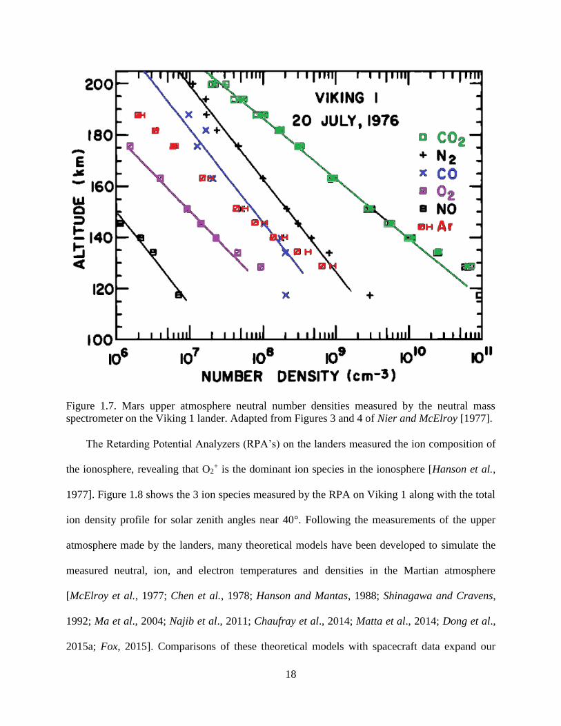
Figure 1.7. Mars upper atmosphere neutral number densities measured by the neutral mass

spectrometer on the Viking 1 lander. Adapted from Figures 3 and 4 of Nier and McElroy [1977].

....................................................................................................................................................... 18

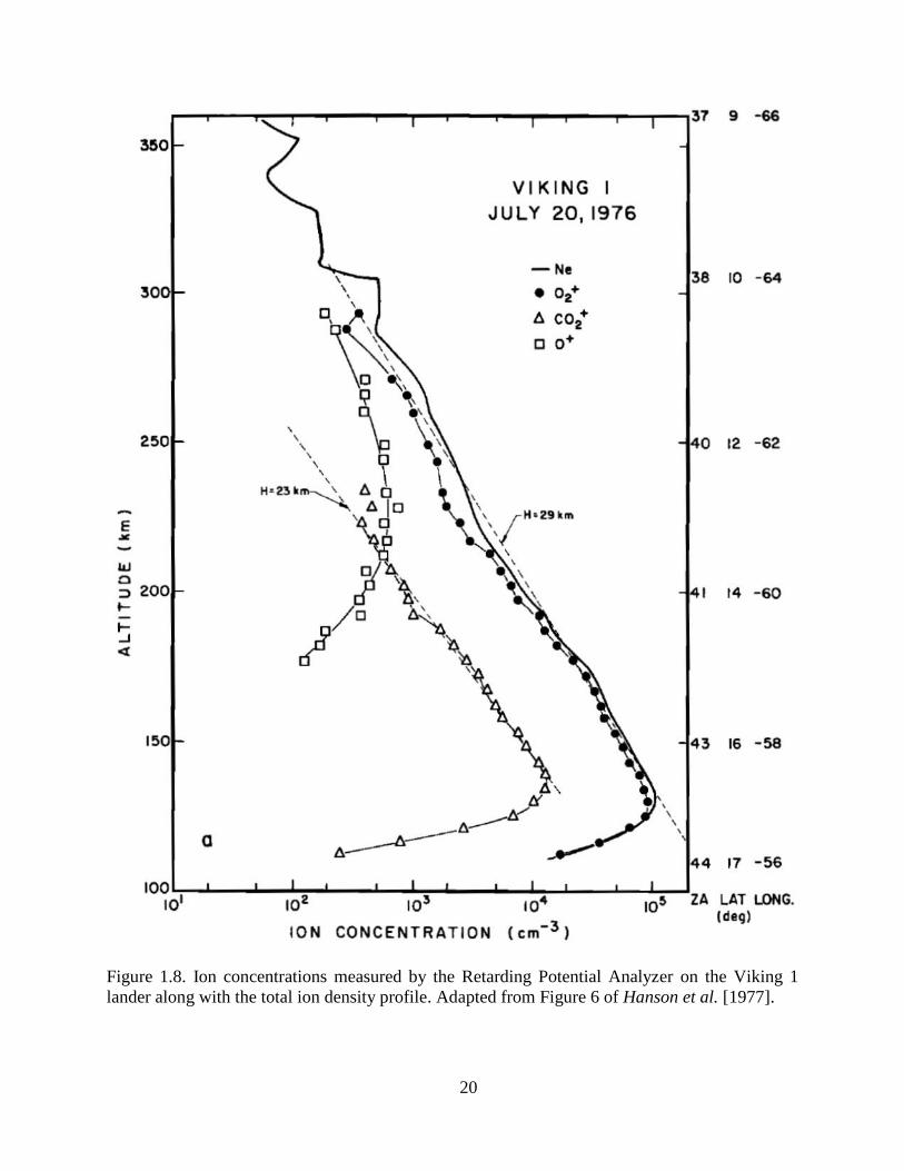
Figure 1.8. Ion concentrations measured by the Retarding Potential Analyzer on the Viking 1

lander along with the total ion density profile. Adapted from Figure 6 of Hanson et al. [1977]. 20

ix

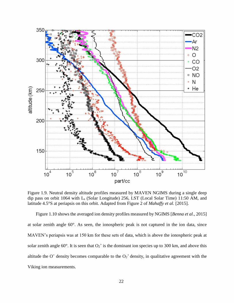
Figure 1.9. Neutral density altitude profiles measured by MAVEN NGIMS during a single

deep dip pass on orbit 1064 with Ls (Solar Longitude) 256, LST (Local Solar Time) 11:50 AM,

and latitude 4.5°S at periapsis on this orbit. Adapted from Figure 2 of Mahaffy et al. [2015]. ... 22

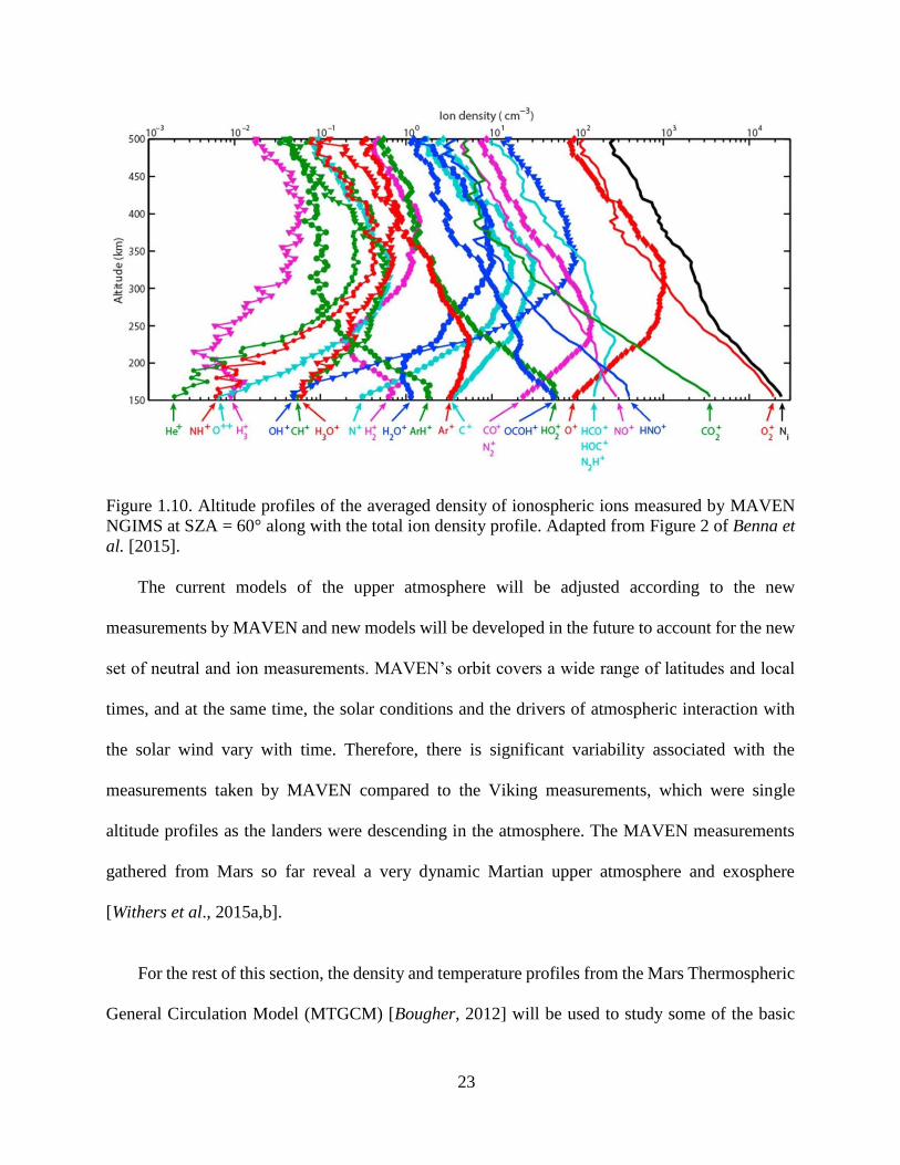
Figure 1.10. Altitude profiles of the averaged density of ionospheric ions measured by

MAVEN NGIMS at SZA = 60° along with the total ion density profile. Adapted from Figure 2 of

Benna et al. [2015]. ....................................................................................................................... 23

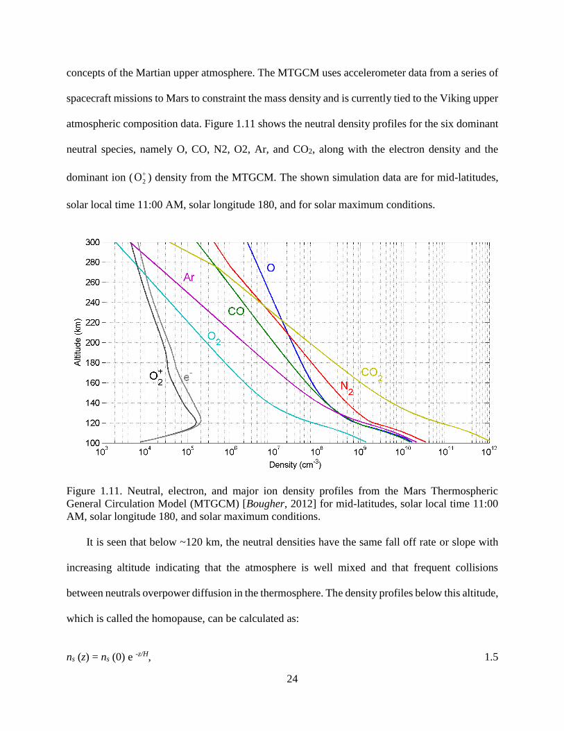
Figure 1.11. Neutral, electron, and major ion density profiles from the Mars Thermospheric

General Circulation Model (MTGCM) [Bougher, 2012] for mid-latitudes, solar local time 11:00

AM, solar longitude 180, and solar maximum conditions. ........................................................... 24

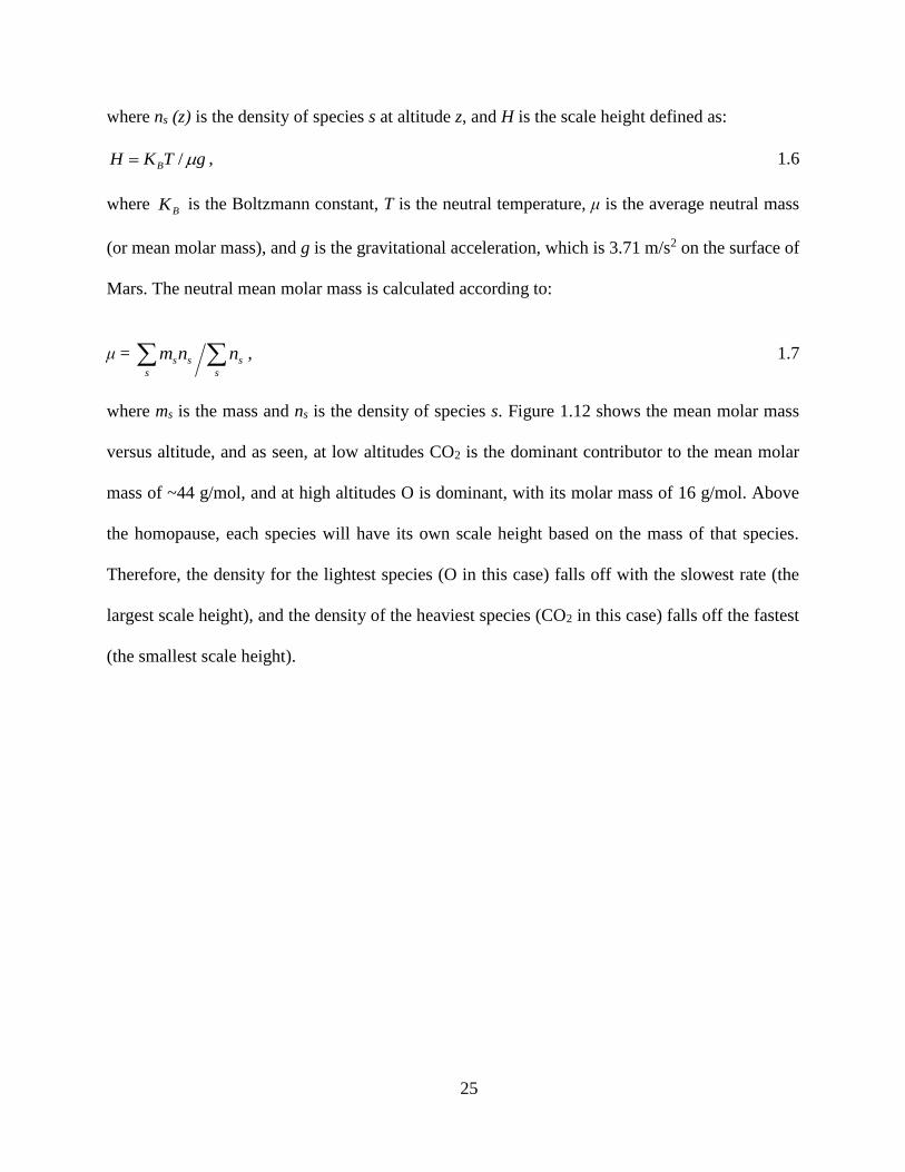
Figure 1.12. Altitude profile of calculated mean molar mass from the MTGCM neutral

densities for mid-latitudes, solar local time 11:00, and solar maximum conditions. .................... 26

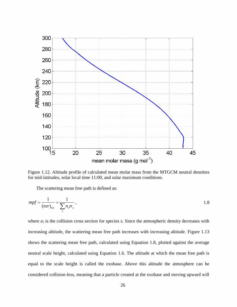
Figure 1.13. Altitude profiles of calculated scattering mean free path as well as the average

neutral scale height from the MTGCM neutral densities for mid-latitudes, solar local time 11:00

AM, solar longitude 180, and solar maximum conditions. ........................................................... 27

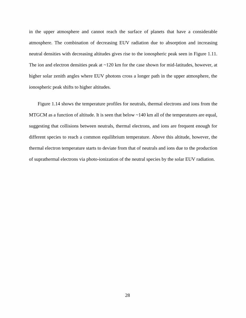
Figure 1.14. Neutral, thermal electron and ion temperature profiles from the MTGCM for mid-

latitudes, solar local time 11:00, and solar maximum conditions. ................................................ 29

Figure 1.15. MAVEN spacecraft with its science instruments onboard. Courtesy: NASA. . 31

Figure 1.16. Science instruments that are carried onboard MAVEN, before being assembled

on the spacecraft. Courtesy: NASA. ............................................................................................. 32

Figure 1.17. MAVEN’s orbital trajectory crosses different regions and boundaries

surrounding Mars, from the upstream undisturbed solar wind into the magneto-sheath, the

magnetic pileup region, and in the wake. At each part of the orbit different instruments take

measurements in different modes that are specific to each region. Courtesy: NASA. ................. 33

Figure 1.18. MAVEN’s orbit precesses in time to allow for a complete sampling of different

regions throughout the science phase of the mission. Courtesy: NASA. ..................................... 34

Figure 1.19. SWIA, SWEA, and MAG measurements of the solar wind and the Martian

plasma parameters during 16 December 2014. The first and second panels are MAVEN’s altitude

and position, respectively depicting the 4.5-hour period of the orbit. The third, fourth, and fifth

panels are SWIA’s ion energy spectra, and the derived ion densities and velocities, respectively.

The sixth panel is SWEA’s electron energy spectra, and the last panel is MAG’s measurements of

the magnetic field. ......................................................................................................................... 35

Figure 2.1. Density profiles for the 6 neutral species as well as the O2+ and electron densities

from a radial cut of the MTGCM for mid-latitudes, solar local time 11:00 AM, solar longitude 180,

and solar minimum (dashed line) and maximum (solid line) conditions...................................... 47

x

Figure 2.2. Neutral, ion, and electron temperature profiles from a radial cut of the MTGCM

for mid-latitudes, solar local time 11:00 AM, solar longitude 180, and solar minimum (dashed line)

and maximum (solid line) conditions. .......................................................................................... 48

Figure 2.3. Production rate of hot oxygen atoms as a function of altitude for solar maximum

(solid line) and minimum (dashed line) conditions with temperature and density inputs from the

MTGCM. ...................................................................................................................................... 51

Figure 2.4. Production rate of hot O atoms as a function of altitude and nascent energy for

solar maximum conditions. ........................................................................................................... 53

Figure 2.5. Production rate of hot O atoms as a function of altitude and nascent energy for

solar minimum conditions............................................................................................................. 54

Figure 2.6. Hot oxygen up and down fluxes as a function of altitude for 1 eV, 3 eV, and 5 eV

atoms calculated using the two-stream code for solar max conditions. ........................................ 58

Figure 2.7. Hot oxygen up and down fluxes as a function of energy at 250 km calculated using

the two-stream code for solar max conditions. ............................................................................. 59

Figure 2.8. Hot oxygen up and down fluxes as a function of energy at 150 km calculated using

the two-stream code for solar max conditions. ............................................................................. 60

Figure 2.9. Hot oxygen up-flux versus energy and altitude calculated using the two-stream

code for solar max conditions. ...................................................................................................... 61

Figure 2.10. Hot oxygen down-flux versus energy and altitude calculated using the two-stream

code for solar max conditions. ...................................................................................................... 62

Figure 2.11. Hot oxygen up-fluxes at 300 km for solar maximum (solid line) and minimum

(dashed line) conditions. ............................................................................................................... 64

Figure 2.12. Hot oxygen energy distributions at 300 km for solar maximum (solid line) and

minimum (dashed line) conditions................................................................................................ 65

Figure 2.13. Hot oxygen exospheric density profiles versus radial distance calculated by the

Liouville code for solar maximum (solid line) and minimum (dashed line) conditions. ............. 67

Figure 2.14. Hot oxygen energy distributions at 300 km for solar maximum conditions,

separated in energy for the escaping and bound parts of the distribution. Adapted from Figure 2 of

Rahmati et al. [2014]. ................................................................................................................... 68


Liouville code for solar maximum conditions. The total density (solid line) as well as the escaping

(dashed line) and bound (dotted-dashed line) densities are shown. The range of altitudes associated

with MAVEN’s orbit around Mars is also shown. The density estimated from Phobos-2 energetic

xi

oxygen pickup ion data [Cravens et al., 2002] is shown by the circle. Adapted from Figure 3 of

Rahmati et al. [2014]. ................................................................................................................... 69

Figure 2.16. Energy dependence of total cross sections for collisions of the incident O with

background CO2 (solid line) and O (dashed line). ........................................................................ 72

Figure 2.17. Hot oxygen up fluxes at 300 km for solar maximum conditions calculated by the

two-stream code using energy independent (solid line), and energy dependent (dashed line) cross

sections. ......................................................................................................................................... 73

Figure 2.18. Solid line: Angular dependence of the “differential” cross section for O-O

collisions at 3 eV, adapted from Kharchenko et al. [2000]. Dashed line: The functional fit to the

differential cross section. .............................................................................................................. 74

Figure 2.19. Total O-O cross section, calculated by integrating the differential cross section

starting from an arbitrary cut-off angle, θmin, to total backscattering, θ = 180°. Solid line: numerical

integration of Kharchenko et al. [2000] values. Dashed line: Analytical integration of the fit

function. ........................................................................................................................................ 76

Figure 2.20. Schematic of the collision geometry used in the Monte-Carlo calculation of

forward and backscattering probabilities and energy losses for use in the two-stream code. ...... 78

Figure 2.21. Hot O trajectories for satellite, ballistic and escape trajectories at Mars. ......... 81

Figure 2.22. Distribution functions of hot O at 300 km from the two-stream (solid line) and

the Monte-Carlo (dashed line) calculations. ................................................................................. 84

Figure 2.23. Hot O escape probability versus the production altitude and the nascent energy

of hot O atoms for solar maximum conditions. ............................................................................ 88

Figure 2.24. Escaping production rate versus the production altitude and the nascent energy

of hot O atoms for solar maximum conditions. ............................................................................ 89

Figure 3.1. Mars exospheric profiles of neutral oxygen atoms, adapted from Rahmati et al.

[2014] and hydrogen atoms, adapted from Feldman et al. [2011]. .............................................. 92

Figure 3.2. Photo-ionization cross sections for oxygen atoms, adapted from Angel and Samson

[1988] and hydrogen atoms, adapted from http://phidrates.space.swri.edu................................. 95

Figure 3.3. Daily averaged solar photon irradiance constructed by FISM for 3 February 2015

as constrained by the EUVM measurements at Mars. .................................................................. 97

Figure 3.4. Daily averaged solar photon flux constructed by FISM for 3 February 2015 as

constrained by the EUVM measurements at Mars. ...................................................................... 98

xii

Figure 3.5. Electron impact cross sections for oxygen and hydrogen atoms, adapted from

Cravens et al. [1987]................................................................................................................... 103

Figure 3.6. A 130 min period of the measurements made by the SWIA and SWEA instruments

starting at 05:50 UTC on 2 February 2015, when MAVEN was in the upstream, undisturbed solar

wind, as well as the calculated ionization frequencies for different ionization processes for oxygen

and hydrogen atoms in the exosphere. Individual panels are explained in the text. ................... 105

Figure 3.7. Energy fluxes of electrons and ions for 06:50 UTC on 2 February 2015, measured

by MAVEN SWIA and SWEA, respectively. ............................................................................ 107

Figure 3.8. Fluxes of electrons and ions for 06:50 UTC on 2 February 2015, measured by

MAVEN SWIA and SWEA, respectively. ................................................................................. 108

Figure 3.9. Typical pickup oxygen and hydrogen ion trajectories upstream of Mars. The

directions of the solar wind velocity, the magnetic field, the motional electric field, and the drift

velocity are also shown. .............................................................................................................. 115

Figure 3.10. Birth curves for oxygen (red) and hydrogen (blue) pickup ions that reach a

sampling point at 6200 km upstream of Mars calculated by the pickup ion code for Usw = 400

km/s, and By = 5 nT. .................................................................................................................... 117

Figure 3.11. Differential fluxes of hydrogen and oxygen pickup ions 6200 km upstream of

Mars, assuming Usw = 400 km/s, and By = 5 nT. ........................................................................ 118

Figure 3.12. Pickup ion ring-beam distribution in velocity space for a solar wind velocity of

400 km/s and a magnetic field in the +Y direction. .................................................................... 119

Figure 3.13. Constant energy contours (brown dashed circles) overlaid on top of the pickup

ion ring-beam distribution (colored solid circle). The portion of the ring distribution between the

two highest energy bins and close to Emax is colored in red. ....................................................... 120

Figure 3.14. Birth points (thick curve) for oxygen pickup ions reaching a sampling point 6200

km upstream of Mars with the colors representing the energy of oxygen pickup ions at the time

they reach the sampling point. Also shown are three sample trajectories (thin curves) for oxygen

pickup ions that are born on the “pickup birth curve” and reach the sampling point with the color

on each trajectory representing the pickup oxygen instantaneous energy at each point on their

respective trajectories.................................................................................................................. 121

Figure 3.15. Pickup oxygen ring distribution for solar wind speeds of 300 km/s, 400 km/s, and

500 km/s, and for a magnetic field in the +Y direction. .............................................................. 122

Figure 3.16. Birth points for oxygen pickup ions that reach a point 6200 km upstream of Mars

for solar wind speeds of 300 km/s, 400 km/s, and 500 km/s, and for By = 5 nT. ....................... 123

xiii

Figure 3.17. Differential fluxes of oxygen pickup ions versus energy for solar wind speeds of

300 km/s, 400 km/s, and 500 km/s, and for By = 5 nT. ............................................................... 124


for a solar wind speed of 400 km/s, and for By = 1 nT, 5 nT, and 20 nT. ................................... 125

Figure 3.19. Differential fluxes of oxygen pickup ions 6200 km upstream of Mars for a solar

wind speed of 400 km/s, and for By = 1 nT, 5 nT, and 20 nT. .................................................... 126

Figure 3.20. Pickup oxygen ring distribution for a solar wind speed of 400 km/s, with a

magnetic field on the XY plane, and for θUB = 30°, 90°, and 120°.............................................. 127


for a solar wind speed of 400 km/s, with a magnetic field on the XY plane equal to B = 5 nT, and

for θUB = 30°, 90°, and 120°........................................................................................................ 128

Figure 3.22. Differential fluxes of oxygen pickup ions 6200 km upstream of Mars for a solar

wind speed of 400 km/s, with a magnetic field on the XY plane equal to B = 5 nT, and for θUB =

30°, 90°, and 120°. ...................................................................................................................... 129

Figure 4.1. Placement and look directions of SEP sensors mounted on MAVEN, each

containing two double-ended telescopes that have perpendicular look directions. Adapted from

Figure 3 of Larson et al. [2015]. ................................................................................................. 133

Figure 4.2. Schematic of the electron and ion telescopes showing the configuration of the foil,

open, and thick detectors as well as the placement of the attenuators, the collimators, the electron

repelling magnet, and the ion stopping foil. Courtesy of Davin Larson. .................................... 134

Figure 4.3. Simulated energy matrix for SEP1F and SEP2F, depicting the deposited energy

vs. the incident energy of oxygen pickup ions. Courtesy of Robert Lillis.................................. 135

Figure 4.4. Fraction of oxygen pickup ions that deposit at least 11 keV in SEP, and are

therefore detected, as a function of their incident energy. Adapted from Figure 6 of Rahmati et al.

[2014]. ......................................................................................................................................... 136

Figure 4.5. Contours of the maximum energy of oxygen pickup ions in the solar wind as a

function of Usw and θUB. Also shown are the lower energy detection limit for SEP and also the

upper energy detection limits for the SWIA and STATIC instruments on MAVEN. Adapted from

Figure 1 of Rahmati et al. [2015]................................................................................................ 137

Figure 4.6. Simulated effective detection area for SEP as a function of polar and azimuth

entrance angles. Courtesy of Davin Larson. ............................................................................... 138

Figure 4.7. Solar wind speeds (1st panel) and densities (2nd panel) measured by SWIA, as well

as the IMF magnitude (3rd panel) measure by MAVEN MAG (magnetometer) during 1-30

December 2014. .......................................................................................................................... 140

xiv

Figure 4.8. Model-data comparison of SEP-detected oxygen pickup ions for part of orbit 343.

The panels are described in the text. Adapted from Figure 3 of Rahmati et al. [2015]. ............. 141

Figure 4.9. SEP2F measured (red) and modeled (blue) count rates for 2 December 2014, 15:00

UTC. The incident maximum energy (Emax) and the corresponding deposited energy full width at

half maximum (FWHM = ΔE) associated with Emax are also shown. Adapted from Figure 4 of

Rahmati et al. [2015]. ................................................................................................................. 143


The panels are described in the text. Adapted from Figure 5 of Rahmati et al. [2015]. ............. 145


The panels are described in the text. ........................................................................................... 146

Figure 4.12. Birth points of oxygen pickup ions on the “pickup ion birth curve” for 3

December 2014, 22:20 UTC. Included are the look directions of SEP1F (blue) and SEP2F (red) as

well as the directions of the solar wind velocity, the magnetic field, and the motional electric field.

The parts of the pickup ion birth curve that enter SEP1F and SEP2F are colored in blue and red,

respectively, and two sample oxygen pickup ion trajectories are depicted in green. ................. 148

Figure 4.13. Pickup ion ring-beam distribution in velocity space for 3 December 2014, 22:20

UTC. Included are the reversed look directions of SEP1F (blue) and SEP2F (red) as well as the

directions of the solar wind velocity, the magnetic field, the motional electric field, and the drift

velocity. The parts of ring distribution that enter SEP1F and SEP2F are colored in blue and red,

respectively. ................................................................................................................................ 149

Figure 4.14. SEP1F and SEP2F flux spectra for 3 December 2014, 22:20 UTC. The blue curve

is the differential flux (in cm-2 s-1 keV-1) of all pickup oxygen ions reaching MAVEN. The green

curve is the part of the flux that is within each SEP’s FOV, convolved with the detector effective

area, giving it units of s-1 keV-1. The cyan curve is the modeled count rates in Hz, after the green

curve is convolved with the energy matrix of SEP, and then binned similar to SEP’s energy table.

The red curve is SEP’s data in Hz. ............................................................................................. 150

Figure 4.15. Model-data comparison of SEP-detected oxygen pickup ions for part of orbit 848

during the passage of the 8 March 2015 ICME. ......................................................................... 152

Figure 4.16. Look directions of SWIA for the coarse data products. Adapted from Figure 9 of

Halekas et al. [2013]. .................................................................................................................. 155

Figure 4.17. The elevation coverage of SWIA as a function of ion energy. Below 5 keV, the

elevation coverage is ±45°. Between 5 keV and 25 keV the elevation coverage is inversely

proportional to energy and reaches ±9° at 25 keV. ..................................................................... 156

Figure 4.18. Model-data comparison of 1D spectra for SWIA-detected oxygen and hydrogen

pickup ions for part of orbit 438. The panels are explained in the text. ..................................... 158

xv

Figure 4.19. Data spectrograms for all of the look directions of SWIA with its 4 elevation

channels separated horizontally, and its 16 anodes, separated vertically for part of orbit 438. The

Solar wind is mainly seen in the middle four look directions. Solar wind ions that scatter in the

instrument are seen as ghost counts uniformly spread among all look directions. The rest of what

is seen is pickup hydrogen and oxygen ions. .............................................................................. 161

Figure 4.20. Oxygen and hydrogen pickup ion model spectrograms for all of the look

directions of SWIA with its 4 elevation channels separated horizontally, and its 16 anodes,

separated vertically for part of orbit 438..................................................................................... 162

Figure 4.21. Model-data comparison of SWIA-detected oxygen and hydrogen pickup ions for

one of the look directions of SWIA (rightmost column of Figure 4.19 and Figure 4.20, panel 11

from top) for part of orbit 438. Lower energy fluxes correspond to pickup hydrogen and higher

energy ones are pickup oxygen. .................................................................................................. 163

Figure 4.22. Model-data comparison of SWIA-detected hydrogen pickup ions for one of the

look directions of SWIA (rightmost column of Figure 4.19 and Figure 4.20, panel 9 from top) for

part of orbit 438. For this look direction no pickup oxygen is detected. .................................... 164


pickup ions for part of orbit 494. The panels are explained in the text. ..................................... 165

Figure 4.24. Data spectrograms for all of the look directions of SWIA with its 4 elevation

channels separated horizontally, and its 16 anodes, separated vertically for part of orbit 494. The

Solar wind is mainly seen in the middle four look directions. Solar wind ions that scatter in the

instrument are seen as ghost counts uniformly spread among all look directions. The rest of what

is seen is pickup hydrogen and oxygen ions. .............................................................................. 167

Figure 4.25. Oxygen and hydrogen pickup ion model spectrograms for all of the look

directions of SWIA with its 4 elevation channels separated horizontally, and its 16 anodes,

separated vertically for part of orbit 494..................................................................................... 168


one of the look directions of SWIA (rightmost column of Figure 4.24 and Figure 4.25, panel 11

from top) for part of orbit 494. Lower energy fluxes correspond to pickup hydrogen and higher

energy ones are pickup oxygen. .................................................................................................. 169

Figure 4.27. Ring distribution of pickup ions in velocity space for 31 December 2014, 10:55

UTC. The directions of the solar wind velocity, the pickup ion drift velocity, the magnetic field,

and the motional electric field are also shown. The blue portion of the ring distribution (for pickup

hydrogen) and the red circles (for pickup oxygen) depict parts of the pickup ion ring distribution

that are within the look direction of SWIA that is shown in Figure 4.26. .................................. 170

Figure 4.28. Model and data energy fluxes for the same look direction shown in Figure 4.26.

The blue and red curves are total model pickup hydrogen and oxygen energy fluxes, respectively.

xvi

The green (SWIA data) and black (pickup ion model) stairs are averaged over a 10-minute time

period centered at 10:55 UTC 31 on December 2014. ............................................................... 172

Figure 4.29. Model-data comparison of SEP-detected oxygen pickup ions as well as 1D

spectra for SWIA-detected oxygen and hydrogen pickup ions for part of orbit 501. The panels are

explained in the text. ................................................................................................................... 174

Figure 4.30. Model-data comparison of SEP-detected oxygen pickup ions as well as SWIA-

detected oxygen and hydrogen pickup ions in one anode of SWIA for part of orbit 336. The panels

are explained in the text. ............................................................................................................. 176

Figure 4.31. Model-data comparisons for SWIA and SEP2F for 1 December 2014, 07:00

UTC. The SWIA data and model results are for the same look direction shown in Figure 4.30.

..................................................................................................................................................... 177


one of the look directions of SWIA for part of orbit 570. Lower energy fluxes correspond to pickup

hydrogen and higher energy ones are pickup oxygen. ................................................................ 179

Figure 5.1. Typical flux of oxygen pickup ions calculated by the pickup ion model and

separated for the bound and escaping parts of the Martian hot oxygen exosphere. Adapted from

Figure 5 of Rahmati et al. [2014]................................................................................................ 183

Figure 5.2. Methodology for testing and constraining models of hot oxygen escape using SEP

pickup oxygen model-data comparisons. Adapted from Figure 1 of Rahmati et al. [2014]. ..... 184

1

1 Introduction

Mars has been the subject of human fascination for years, due to its similarities with our own

Earth. It has been the subject of questions like “can life exist or has life ever existed on Mars” or

“is there water on Mars”. The earliest documented efforts in studying the atmosphere of Mars date

back to the late 18th century, with William Herschel’s observations of the occultation of stars by

Mars. Later in the 1830s, James South also made similar observations both arriving at no

conclusion on the existence of a considerable atmosphere attached to Mars. In the mid-19th century,

spectroscopic observations of Mars were conducted in hopes of finding evidence for an atmosphere

on Mars and the presence of water vapor in the atmosphere to explain the Martian polar caps. By

the early 20th century, it was believed that Mars had a thin atmosphere unable to support water on

the surface in the liquid form, and that the polar caps were likely mainly composed of frozen

carbon dioxide and/or water.

During the second half of the 20th century, there were numerous attempts to send spacecraft

to Mars to study its geology and atmosphere, more than half of which failed to achieve their goal.

The first successful mission was the Mariner 4 flyby of Mars in 1965 followed by Mariners 6 and

7 flybys of the planet in 1969. The Mariner flybys provided the first images of the Martian surface

from deep space and enabled studying the extended hydrogen exosphere of Mars. Later in 1971,

Mariner 9, Mars 2, and Mars 3 successfully entered orbit around Mars; the latter spacecraft also

carried a lander that marked the first successful soft landing on the Martian surface. The Viking 1

and 2 orbiters and landers launched in 1975 and were the next successful missions to Mars. The

Viking landers provided the first in situ measurements of the Martian upper atmospheric

2

composition, densities and temperatures [Hanson et al., 1977; Nier and McElroy, 1977; Hanson

and Mantas, 1988].

The Phobos-2 mission to Mars that arrived in January 1989 carried plasma detectors as well

as magnetometers that allowed comprehensive study of the interaction of the solar wind with Mars

[Sagdeev and Zakharov, 1989]. However, Phobos-2 only operated for just below two months

before it failed and the mission was partially successful. The Mars Global Surveyor and the Mars

Express spacecraft each carried partial particles and fields instruments. The magnetometer and

electron reflectometer on the Mars Global Surveyor spacecraft carried out a global mapping of the

magnetic structure of Mars. No global magnetic field was found, and crustal magnetic fields were

discovered, mostly over the Martian southern hemisphere [Acuna et al., 1999]. The Mars Express

spacecraft is still operating and is carrying a plasma detector that measures the escape rate of ions

from Mars [Barabash et al., 2007]. The lack of the global magnetic field on Mars means that the

solar wind can directly interact with the upper atmosphere and drive ion escape via ionization,

heating, sputtering, and the pickup process.

The Mars Atmosphere and Volatile EvolutioN (MAVEN) mission to Mars [Jakosky et al.,

2015a] is the first spacecraft that carries a full suite of plasma particles and fields as well as remote

sensing instruments, aimed at understanding the interaction of the solar wind with the upper

atmosphere, and characterizing the role that escape of volatiles has played in changing the Martian

climate. In this chapter the evidence of the presence of water on Mars is presented, the processes

leading to the disappearance of water through atmospheric escape are described, and our current

knowledge of the upper atmosphere of Mars and its interaction with the solar wind via observations

and modeling is discussed. Later in the chapter, the role of the MAVEN mission to Mars in

3

improving our knowledge of the Mars plasma environment and volatile escape is explained and

the MAVEN’s instrumentation used to achieve this goal is described. Finally, the research carried

out in this dissertation is explained and the parts that are new and original work are described.

1.1 Evidence of Water on Mars

Geological and isotopic evidence suggests that in the distant past water existed on the surface

of Mars and that the atmosphere was much thicker [e.g., Goldspiel and Squyres, 1991; Jakosky et

al., 1994; Carr, 1996; Haberle, 1998; Malin and Edgett, 2003]. Images of the Martian surface

taken by the Mars orbiters show runoff channels that look like river drainage systems as well as

features that are similar to riverbeds on Earth, suggesting that liquid water used to flow on the

surface of Mars. There is geological evidence for ancient lakes filling impact craters and minerals

that form only in the presence of liquid water. The pictures also exhibit signs of precipitation

induced erosion on surface slants. Figure 1.1 shows some of these features in photos taken by the

Viking Orbiter, the Mars Global Surveyor, and the Mars Reconnaissance Orbiter.

4

Figure 1.1. top-left: The recurring slope lineae features imaged by the Mars Reconnaissance

Orbiter spacecraft, indicative of seasonal salty water flows on warm slopes. top-right: The Viking

Orbiter image of the valley network on Mars possibly caused by flowing water similar to stream

drainage patterns on Earth. bottom-left: The largest outflow channel on Mars at some places

reaching 2.5 km deep, believed to be formed by erosion of running water. bottom-right: The Mars

Global Surveyor image of a distributary fan-delta on Mars, evidence for the flow of water and the

subsequent sediment deposition. All images courtesy of NASA.

The landers and rovers on the surface have also sent back data on the composition and isotopic

ratios of the surface elements as well as images of the Martian rock and soil features. Analysis of

geological data reveals that water used to exist on the surface up until 3.7 billion years ago [e.g.,

Jakosky and Phillips, 2001; Solomon et al., 2005; Fassett and Head, 2011; Leshin et al., 2013].

5

Images taken from the surface show sedimentary rock formations, a sign for the existence of lakes

and water deposition on the surface; therefore, water is believed to have been abundant on the

surface in the past. Figure 1.2 shows the sedimentary rocks that are believed to be formed by

deposition due to standing water in the lakes.

Figure 1.2. top-left: Image of layers of sediment at Burns Cliff inside the Endurance Crater taken

by the Opportunity rover at Mars. top-right: Curiosity rover image of layers of rock on Mars.

bottom-left: Curiosity rover image of “cross-bedding” in the layers of a Martian rock, indicating

the presence of flowing water during deposition. bottom-right: Curiosity rover image of a layered

Martian outcrop exhibiting signs of cross-bedding. All images courtesy of NASA.

Water is also present as ice in the polar caps, but the current Martian atmosphere is thin and

unable to support water in liquid form on the surface. The bulk of the Martian north and south

polar caps is water ice, with layers of CO2 depositing on top during winter seasons. This seasonal

freezing and sublimating of CO2 can change the atmospheric pressure by up to 30%, since the

atmosphere is mainly composed of CO2. Although there is ample evidence for the presence of

abundant liquid water on Mars in the past, over time liquid water has disappeared from the surface

6

of Mars and the Martian climate has completely changed. Water could have either gone down

below the surface into the crust or been absorbed by the rocks, or gone up in the atmosphere and

escaped to space.

Since water molecules are composed of oxygen and hydrogen atoms, by measuring the current

escape flux of oxygen and hydrogen atoms from the atmosphere, and through modeling, the

amount of water that has escaped from the planet over the last few billion years can be estimated.

One of the goals of the MAVEN mission to Mars is to quantify the escape of volatiles to space by

measuring the current rate of atmospheric escape and its dependence on the drives of escape. By

going back in time we can extrapolate the escape rates, given some knowledge of the time

dependence of the drivers of escape, and integrate the loss to space to find out how much water in

total has been lost through atmospheric escape from Mars.

1.2 Atmospheric Escape

Planetary atmospheres are attached to their host planets by the gravitational pull of the planet

on atmospheric atoms and molecules. The escape velocity on a planet is given by:

R

G M = Vesc

2, 1.1

where G is the gravitational constant equal to:

G = 6.67 × 10-11 m3 kg-1 s-2, 1.2

M is the mass of the planet, and R is the radius of the planet. For Mars,

M = 6.4 × 1023 kg, 1.3

and

7

R = RM = 3,400 km, 1.4

giving an escape velocity of 5.0 km/s on Mars. For comparison, the escape velocity on Earth is

11.2 km/s, and on Venus is 10.3 km/s. Any particle in the Martian atmosphere that gains a velocity

greater than 5 km/s can escape from the planet, unless it has a downward velocity or it encounters

enough collisions with background neutral species that result in energy loss, bringing its velocity

below 5 km/s. Atmospheric loss can take place through a number of different mechanisms. The

processes involved in atmospheric escape from Mars have been extensively investigated in the

past few decades [e.g., Lundin et al., 1989; Brain and Jakosky, 1998; Chassefière and Leblanc,

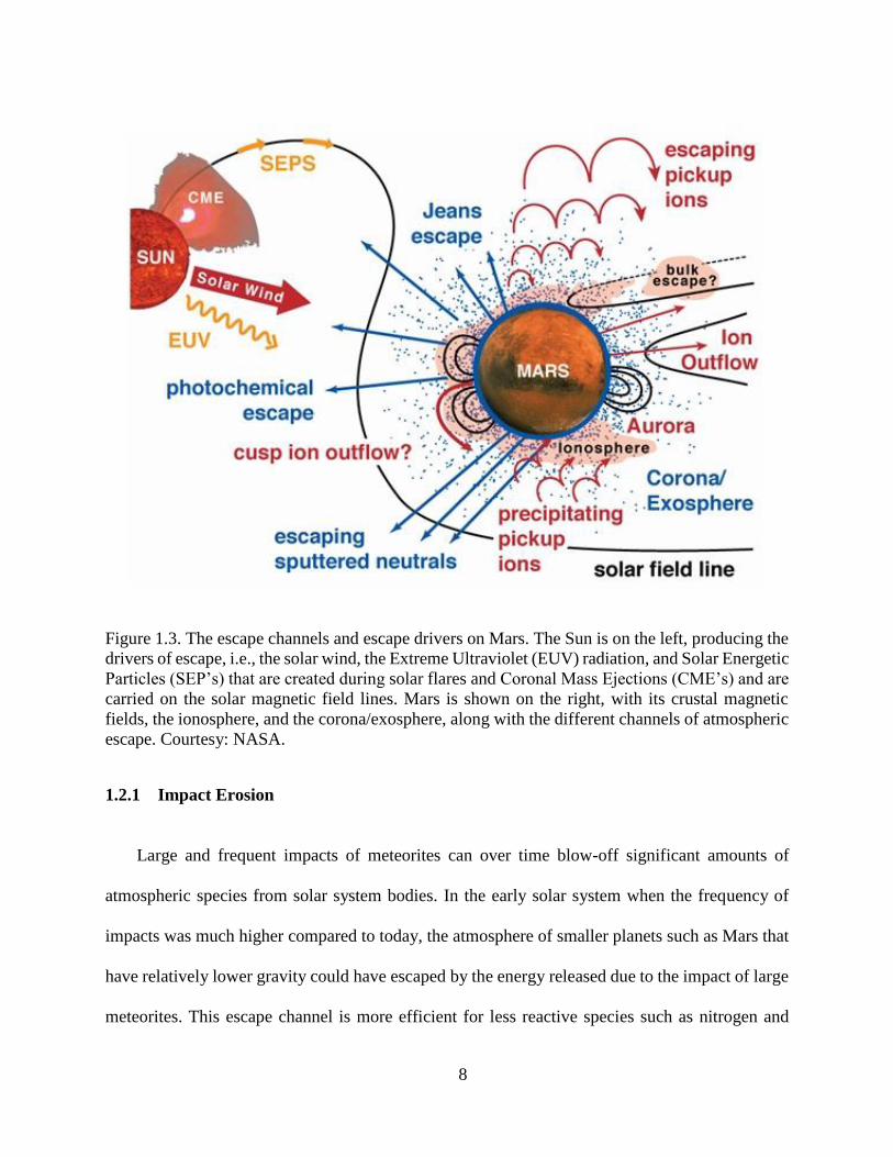
2004; Bougher et al., 2009]. Figure 1.3 shows a schematic of the escape processes and their drivers

on Mars and the following sections give a brief description for each process.

8

Figure 1.3. The escape channels and escape drivers on Mars. The Sun is on the left, producing the

drivers of escape, i.e., the solar wind, the Extreme Ultraviolet (EUV) radiation, and Solar Energetic

Particles (SEP’s) that are created during solar flares and Coronal Mass Ejections (CME’s) and are

carried on the solar magnetic field lines. Mars is shown on the right, with its crustal magnetic

fields, the ionosphere, and the corona/exosphere, along with the different channels of atmospheric

escape. Courtesy: NASA.

1.2.1 Impact Erosion

Large and frequent impacts of meteorites can over time blow-off significant amounts of

atmospheric species from solar system bodies. In the early solar system when the frequency of

impacts was much higher compared to today, the atmosphere of smaller planets such as Mars that

have relatively lower gravity could have escaped by the energy released due to the impact of large

meteorites. This escape channel is more efficient for less reactive species such as nitrogen and

9

noble gases that can remain in the atmosphere, compared to volatiles like H2O or CO2 that can be

sequestered and adsorbed in rocks [Carr, 1987].

1.2.2 Jeans Escape

The velocity or energy distribution of atmospheric neutrals follows a Maxwell–Boltzmann

distribution in which a few particles have very small and very large speeds, and most of the

particles are distributed about an equilibrium thermal velocity or energy. This equilibrium is

achieved due to frequent collisions between the atmospheric species. In Jeans escape, particles

from the high velocity tail of the Maxwell–Boltzmann distribution can reach the escape velocity

and overcome the planet’s gravitational attraction. This process is only effective for light species

such as hydrogen and helium for which the escape energy is low. For example, the escape energy

for a hydrogen atom is 0.125 eV on Mars. The neutral temperature in the upper atmosphere can

reach 300 K, giving hydrogen atoms a thermal energy of 0.025 eV. The Maxwell-Boltzmann

distribution maintains that a small portion of hydrogen atoms will have energies that are more than

5 times their thermal energy, and therefore above the escape energy on Mars. That portion of

hydrogen atoms can escape from Mars through the Jeans process, and create the extended

hydrogen exosphere of Mars.

1.2.3 Hydrodynamic Escape

In atmospheres with very high temperatures, the bulk of the atmosphere can be blown off as

a result of heavier species being dragged along by the lighter species that are escaping through the

Jeans process. Just like the Jeans escape, hydrodynamic escape is more efficient on planets with

lower gravitational force, and therefore lower escape velocity or energy. Compared to Jeans escape

10

in which only particles in the high energy tail of the Maxwell-Boltzmann distribution escape, in

hydrodynamic escape most of the distribution for light species lies above the escape energy. The

collisions between thermally driven escaping lighter species and the heavier ones are responsible

for the escape of heavier species.

1.2.4 Ion Outflow

The solar wind is the stream of plasma flowing away from the Sun, carrying the interplanetary

magnetic field with it. The solar wind is mainly composed of protons and alpha particles as well

as electrons. Every planet in the solar system experiences the solar wind and interacts with it based

on the planet’s atmospheric and magnetic characteristics. The magnetic field of the Earth acts as a

shield, preventing the solar wind from reaching the upper atmosphere and eroding the atmosphere

away. Mars, on the other hand, lacks a global magnetic field and the solar wind can directly interact

with the upper atmosphere and drive off charged particles.

The interaction of the solar wind and its embedded magnetic field with the ionosphere of

planets can lead to the escape of a bulk of ions from the ionosphere. The Phobos-2 and the Mars

Express (MEX) spacecraft both carried instrumentation that observed energetic ions escaping from

Mars and the measured escape rates of oxygen ions range between 1024 s-1 to a few times 1025 s-1

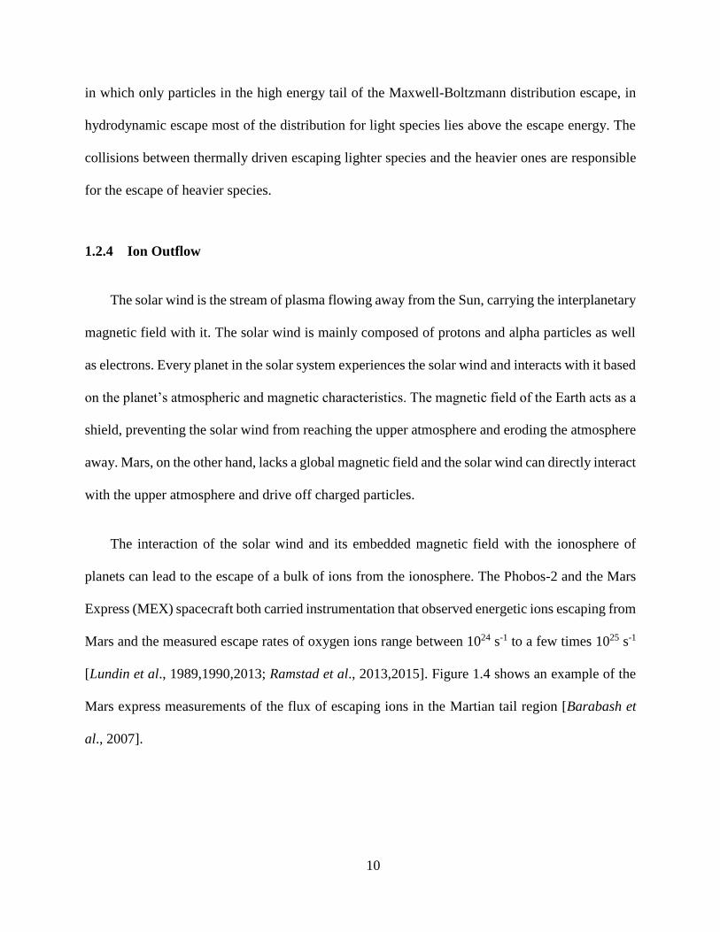
[Lundin et al., 1989,1990,2013; Ramstad et al., 2013,2015]. Figure 1.4 shows an example of the

Mars express measurements of the flux of escaping ions in the Martian tail region [Barabash et

al., 2007].

11

Figure 1.4. Mars Express observation of the flux of escaping ions from Mars. The coordinate

system shown is Mars-Solar-Electric (MSE) in which the X axis points from Mars to the Sun, The

Z axis points in the direction of the motional electric field (E = - Usw × B), and the Y axis completes

the right-handed coordinate system. Adapted from Figure 1 of Barabash et al. [2007].

Similar measurements of ion outflow are being taken by MAVEN with a higher temporal and

spatial resolution, in conjunction with other plasma and field measurements that allow for

connecting drivers of escape to escape rates at Mars. Recent measurements by the MAVEN

12

spacecraft indicate a very complex solar wind interaction with the upper atmosphere of Mars and

confirm that part of the ionosphere is being lost due to the solar wind interaction with the

ionosphere [Brain et al., 2015; DiBraccio et al., 2015; Ma et al., 2015]. In one recent study using

MAVEN data, a new plume-like channel of ion escape was identified in which strong fluxes of O+

ions were observed leaving Mars in the direction of the solar wind motional electric field (E = -

Usw × B) with energies above the escape energy [Dong et al., 2015].

1.2.5 Pickup Ions

The exosphere of Mars is very extended and thermal hydrogen and hot oxygen atoms extend

out to several Martian radii. Ionization of these atoms creates ions that react to the magnetic field

of the solar wind and are accelerated via the motional electric field in a process called “pickup”

[Jarvinen and Kallio, 2014]. This acceleration can give pickup oxygen ions enough energy to

overcome the gravity of Mars. Therefore, solar wind interaction with the upper atmosphere of

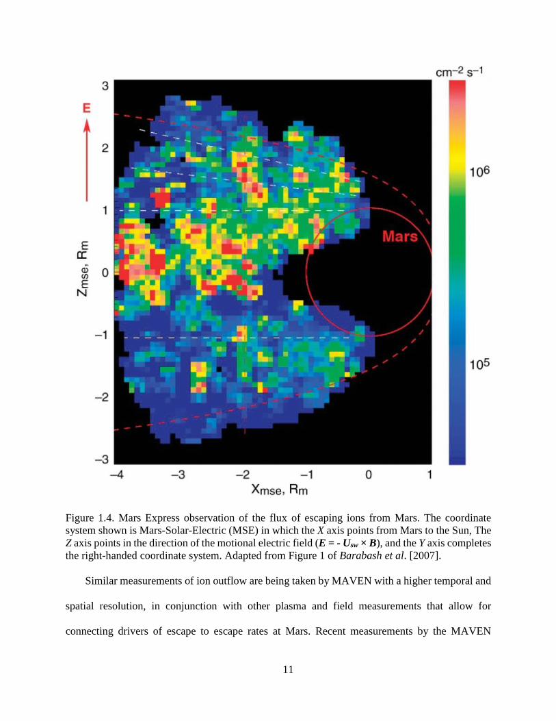
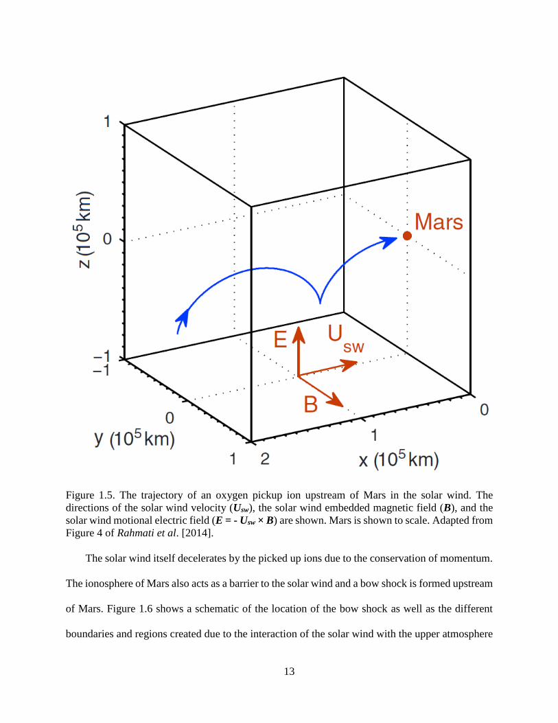
Mars can be a source of escape of oxygen and hydrogen atoms through the pickup process. Figure

1.5 shows a schematic of the motion of an oxygen pickup ion that is created upstream of Mars and

is gyrating downstream back towards Mars. The directions of the solar wind velocity (Usw), the

solar wind embedded magnetic field (B), and the solar wind motional electric field (E = - Usw ×

B) are also shown.

13

Figure 1.5. The trajectory of an oxygen pickup ion upstream of Mars in the solar wind. The

directions of the solar wind velocity (Usw), the solar wind embedded magnetic field (B), and the

solar wind motional electric field (E = - Usw × B) are shown. Mars is shown to scale. Adapted from

Figure 4 of Rahmati et al. [2014].

The solar wind itself decelerates by the picked up ions due to the conservation of momentum.

The ionosphere of Mars also acts as a barrier to the solar wind and a bow shock is formed upstream

of Mars. Figure 1.6 shows a schematic of the location of the bow shock as well as the different

boundaries and regions created due to the interaction of the solar wind with the upper atmosphere

14

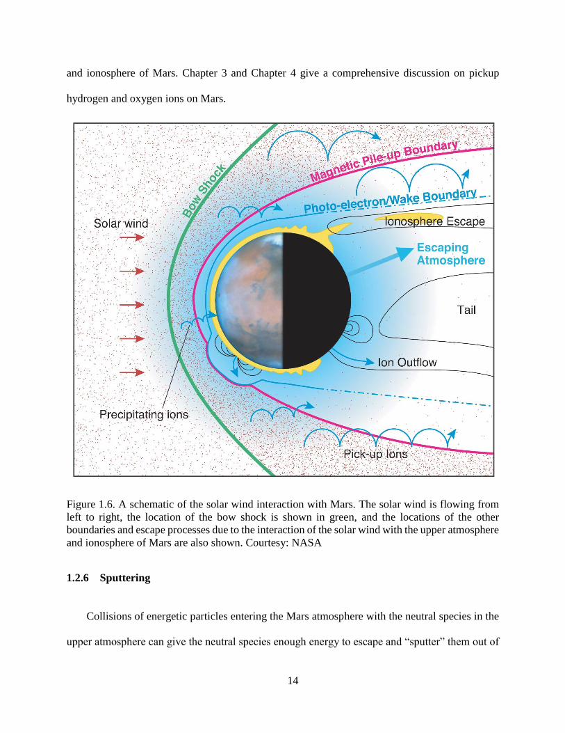
and ionosphere of Mars. Chapter 3 and Chapter 4 give a comprehensive discussion on pickup

hydrogen and oxygen ions on Mars.

Figure 1.6. A schematic of the solar wind interaction with Mars. The solar wind is flowing from

left to right, the location of the bow shock is shown in green, and the locations of the other

boundaries and escape processes due to the interaction of the solar wind with the upper atmosphere

and ionosphere of Mars are also shown. Courtesy: NASA

1.2.6 Sputtering

Collisions of energetic particles entering the Mars atmosphere with the neutral species in the

upper atmosphere can give the neutral species enough energy to escape and “sputter” them out of

15

the atmosphere. The energetic particles driving the sputtering process either come from the Sun

during solar particle events, or are the accelerated pickup ions (mostly oxygen) that re-enter the

upper atmosphere with energies in excess of a few keV. Solar particle events are periods of

intensified flux of energetic particles (protons, alphas, highly ionized carbon and oxygen) during

the passage of Interplanetary Coronal Mass Ejections (ICME’s) or accelerated particles due to

solar flares. These events are more frequent during the peak of the solar activity (solar magnetic

cycle maximum) and can happen as often as a few times a month [Reams, 2004; Jun et al., 2007].

Direct impact of these solar energetic particles with the neutral species in the upper atmosphere of

Mars can increase the sputtering rate [Jakosky et al., 1994].

During the times of elevated solar wind speed, oxygen pickup ions can gain energies as high

as a few hundred keV. The re-impact of these pickup ions with neutral oxygen atoms in the

exosphere of Mars can also sputter the neutrals away [Leblanc et al., 2015]. Modeling efforts

indicate that in the distant past when the solar conditions were more extreme, the sputtering of the

Martian atmosphere due to energetic pickup ions had been one of the major escape channels on

Mars [Luhmann and Kozyra, 1991; Luhmann et al., 1992; Leblanc and Johnson, 2001].

1.2.7 Photo-chemical Escape

Solar ultraviolet photons can ionize the neutral species in the upper atmosphere of planets,

leading to the creation of ionosphere and the consequent photo-chemical reactions. These reactions

can produce non-thermal (hot) particles with energies high enough to escape the planet. One of the

main processes leading to the escape of neutral oxygen atoms from Mars is the photo-chemical

escape, where hot oxygen atoms are created in the Martian ionosphere via the dissociative

recombination of O2+ ions with electrons [Nagy and Cravens, 1988; Fox and Hać, 1997; Kim et

16

al., 1998; Fox and Hać, 2009]. About 70% of oxygen atoms produced in this reaction will have

energies greater than the escape energy of an oxygen atom on Mars (2 eV) and can leave the planet.

These non-thermal atoms will also contribute to a hot oxygen corona (exosphere) of Mars. On

Venus, the escape energy for an oxygen atom is 8 eV, which is above the energy that hot oxygen

atoms gain in the O2+ dissociative recombination reaction. Therefore, on Venus, oxygen does not

escape photo-chemically and the hot O corona of Venus is all bound and is responsible for the

oxygen corona observed via resonantly scattered solar 130.4 nm photons by the Pioneer Venus

Orbiter (PVO) ultraviolet spectrometer [Nagy et al., 1981].

Because of the very low densities in the distant part of the Martian hot O exosphere, where

oxygen atoms are mainly escaping, it is difficult to directly measure the photo-chemical escape

rate of oxygen; therefore, models have to be utilized to calculate the escape rate. The theoretical

models that are used in simulations of photo-chemical escape of oxygen take in the density and

temperature profiles of the atmospheric neutrals and ions and calculate the resulting hot atom

production, flux, distribution, and escape rate. Chapter 2 discusses, in detail, the steps required to

construct the hot O distribution and exospheric densities and escape rates for Mars.

The photo-chemical escape rates predicted by different escape models vary by about 2 orders

of magnitude as summarized in Table 3 of Fox and Hać [2009]. Therefore, it is essential to

constrain the modeled escape rates using observations. Chapters 5 discusses the methodology that

can be used to constrain models of Mars hot O exosphere and photo-chemical escape by comparing

model pickup ion fluxes with MAVEN measurements.

17

1.3 The Upper Atmosphere of Mars

The first in situ measurements of the composition of the Martian upper atmosphere were made

by the Viking 1 and 2 landers in 1976. Neutral, ion, and electron densities and temperatures

measured by different instruments onboard the landers as they were descending down in the

atmosphere have been used in the past few decades to gain a better understanding of the processes

within the thermosphere and the ionosphere of Mars. The measurements of the composition and

structure of Mars’ upper atmosphere by the neutral mass spectrometers flown on the landers

indicate that the main constituents of the Martian atmosphere are carbon dioxide (CO2), molecular

nitrogen (N2), carbon monoxide (CO), and Argon (Ar), with chemically produced atomic oxygen

(O) [Nier and McElroy, 1977]. Figure 1.7 shows the density profiles measured by the neutral mass

spectrometer on the Viking 1 lander. Atomic oxygen (O) was not directly measured by Viking 1

and its density was later deduced by chemical arguments.

18

Figure 1.7. Mars upper atmosphere neutral number densities measured by the neutral mass

spectrometer on the Viking 1 lander. Adapted from Figures 3 and 4 of Nier and McElroy [1977].

The Retarding Potential Analyzers (RPA’s) on the landers measured the ion composition of

the ionosphere, revealing that O2+ is the dominant ion species in the ionosphere [Hanson et al.,

1977]. Figure 1.8 shows the 3 ion species measured by the RPA on Viking 1 along with the total

ion density profile for solar zenith angles near 40°. Following the measurements of the upper

atmosphere made by the landers, many theoretical models have been developed to simulate the

measured neutral, ion, and electron temperatures and densities in the Martian atmosphere

[McElroy et al., 1977; Chen et al., 1978; Hanson and Mantas, 1988; Shinagawa and Cravens,

1992; Ma et al., 2004; Najib et al., 2011; Chaufray et al., 2014; Matta et al., 2014; Dong et al.,

2015a; Fox, 2015]. Comparisons of these theoretical models with spacecraft data expand our

19

knowledge of the geological, physical, and chemical processes involved on the surface and in the

atmosphere of Mars [Withers et al., 2015b].

20

Figure 1.8. Ion concentrations measured by the Retarding Potential Analyzer on the Viking 1

lander along with the total ion density profile. Adapted from Figure 6 of Hanson et al. [1977].

21

Since the conclusion of the Viking program, a number of successful orbiter, lander, and rover

missions to Mars have increased our knowledge of the planet’s surface and atmosphere, but up

until September 2014 when MAVEN arrived at Mars, the Viking data remained the only in situ

measurements of the Martian upper atmosphere composition. MAVEN has been operating in

science mode since mid-November 2014 and has been taking in situ measurement of the upper

atmosphere in different local times and latitudes. Figure 1.9 shows the neutral density profiles

measured by the Neutral Gas and Ion Mass Spectrometer (NGIMS) instrument on MAVEN

[Mahaffy et al., 2015] on orbit 1064 for near noon local solar time and equatorial conditions. As

seen, CO2 is the dominant neutral species below 250 km, and above this altitude the atomic oxygen

density dominates. Comparing Figure 1.7 and Figure 1.9 indicates that there is general agreement

between the Viking and the MAVEN neutral measurements, although they were taken at different

solar activity and locations on the planet.

22

Figure 1.9. Neutral density altitude profiles measured by MAVEN NGIMS during a single deep

dip pass on orbit 1064 with Ls (Solar Longitude) 256, LST (Local Solar Time) 11:50 AM, and

latitude 4.5°S at periapsis on this orbit. Adapted from Figure 2 of Mahaffy et al. [2015].

Figure 1.10 shows the averaged ion density profiles measured by NGIMS [Benna et al., 2015]

at solar zenith angle 60°. As seen, the ionospheric peak is not captured in the ion data, since

MAVEN’s periapsis was at 150 km for these sets of data, which is above the ionospheric peak at

solar zenith angle 60°. It is seen that O2+ is the dominant ion species up to 300 km, and above this

altitude the O+ density becomes comparable to the O2+ density, in qualitative agreement with the

Viking ion measurements.

23

Figure 1.10. Altitude profiles of the averaged density of ionospheric ions measured by MAVEN

NGIMS at SZA = 60° along with the total ion density profile. Adapted from Figure 2 of Benna et

al. [2015].

The current models of the upper atmosphere will be adjusted according to the new

measurements by MAVEN and new models will be developed in the future to account for the new

set of neutral and ion measurements. MAVEN’s orbit covers a wide range of latitudes and local

times, and at the same time, the solar conditions and the drivers of atmospheric interaction with

the solar wind vary with time. Therefore, there is significant variability associated with the

measurements taken by MAVEN compared to the Viking measurements, which were single

altitude profiles as the landers were descending in the atmosphere. The MAVEN measurements

gathered from Mars so far reveal a very dynamic Martian upper atmosphere and exosphere

[Withers et al., 2015a,b].

For the rest of this section, the density and temperature profiles from the Mars Thermospheric

General Circulation Model (MTGCM) [Bougher, 2012] will be used to study some of the basic

24

concepts of the Martian upper atmosphere. The MTGCM uses accelerometer data from a series of

spacecraft missions to Mars to constraint the mass density and is currently tied to the Viking upper

atmospheric composition data. Figure 1.11 shows the neutral density profiles for the six dominant

neutral species, namely O, CO, N2, O2, Ar, and CO2, along with the electron density and the

dominant ion (

2O ) density from the MTGCM. The shown simulation data are for mid-latitudes,

solar local time 11:00 AM, solar longitude 180, and for solar maximum conditions.

Figure 1.11. Neutral, electron, and major ion density profiles from the Mars Thermospheric

General Circulation Model (MTGCM) [Bougher, 2012] for mid-latitudes, solar local time 11:00

AM, solar longitude 180, and solar maximum conditions.

It is seen that below ~120 km, the neutral densities have the same fall off rate or slope with

increasing altitude indicating that the atmosphere is well mixed and that frequent collisions

between neutrals overpower diffusion in the thermosphere. The density profiles below this altitude,

which is called the homopause, can be calculated as:

ns (z) = ns (0) e -z/H, 1.5

25

where ns (z) is the density of species s at altitude z, and H is the scale height defined as:

gTKH B / , 1.6

where BK is the Boltzmann constant, T is the neutral temperature, μ is the average neutral mass

(or mean molar mass), and g is the gravitational acceleration, which is 3.71 m/s2 on the surface of

Mars. The neutral mean molar mass is calculated according to:

μ = s

s

s

ss nnm , 1.7

where ms is the mass and ns is the density of species s. Figure 1.12 shows the mean molar mass

versus altitude, and as seen, at low altitudes CO2 is the dominant contributor to the mean molar

mass of ~44 g/mol, and at high altitudes O is dominant, with its molar mass of 16 g/mol. Above

the homopause, each species will have its own scale height based on the mass of that species.

Therefore, the density for the lightest species (O in this case) falls off with the slowest rate (the

largest scale height), and the density of the heaviest species (CO2 in this case) falls off the fastest

(the smallest scale height).

26

Figure 1.12. Altitude profile of calculated mean molar mass from the MTGCM neutral densities

for mid-latitudes, solar local time 11:00, and solar maximum conditions.

The scattering mean free path is defined as:

s

sstot nnmpf

1

)(

1, 1.8

where σs is the collision cross section for species s. Since the atmospheric density decreases with

increasing altitude, the scattering mean free path increases with increasing altitude. Figure 1.13

shows the scattering mean free path, calculated using Equation 1.8, plotted against the average

neutral scale height, calculated using Equation 1.6. The altitude at which the mean free path is

equal to the scale height is called the exobase. Above this altitude the atmosphere can be

considered collision-less, meaning that a particle created at the exobase and moving upward will

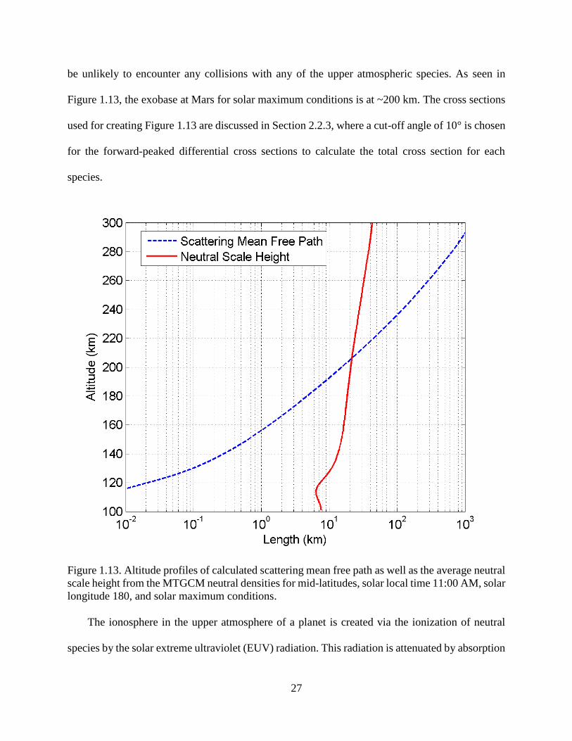
27

be unlikely to encounter any collisions with any of the upper atmospheric species. As seen in

Figure 1.13, the exobase at Mars for solar maximum conditions is at ~200 km. The cross sections

used for creating Figure 1.13 are discussed in Section 2.2.3, where a cut-off angle of 10° is chosen

for the forward-peaked differential cross sections to calculate the total cross section for each

species.

Figure 1.13. Altitude profiles of calculated scattering mean free path as well as the average neutral

scale height from the MTGCM neutral densities for mid-latitudes, solar local time 11:00 AM, solar

longitude 180, and solar maximum conditions.

The ionosphere in the upper atmosphere of a planet is created via the ionization of neutral

species by the solar extreme ultraviolet (EUV) radiation. This radiation is attenuated by absorption

28

in the upper atmosphere and cannot reach the surface of planets that have a considerable

atmosphere. The combination of decreasing EUV radiation due to absorption and increasing

neutral densities with decreasing altitudes gives rise to the ionospheric peak seen in Figure 1.11.

The ion and electron densities peak at ~120 km for the case shown for mid-latitudes, however, at

higher solar zenith angles where EUV photons cross a longer path in the upper atmosphere, the

ionospheric peak shifts to higher altitudes.

Figure 1.14 shows the temperature profiles for neutrals, thermal electrons and ions from the

MTGCM as a function of altitude. It is seen that below ~140 km all of the temperatures are equal,

suggesting that collisions between neutrals, thermal electrons, and ions are frequent enough for

different species to reach a common equilibrium temperature. Above this altitude, however, the

thermal electron temperature starts to deviate from that of neutrals and ions due to the production

of suprathermal electrons via photo-ionization of the neutral species by the solar EUV radiation.

29

Figure 1.14. Neutral, thermal electron and ion temperature profiles from the MTGCM for mid-

latitudes, solar local time 11:00, and solar maximum conditions.

Suprathermal electrons can thermalize via Coulomb collisions with thermal electrons. The

energy exchange between suprathermal electrons and thermal electrons increases the thermal

electron temperature. The energy exchange between thermal electrons and neutrals, on the other

hand, acts as a sink of energy for thermal electrons. Therefore, as the altitude increases and the

density of neutrals decreases, the less frequent collisions between thermal electrons and neutrals

cause the thermal electron temperature to rise. The increase in ion temperature with increasing

30

altitude is also a result of energy exchange between thermal electrons and ions via Coulomb

collisions and the lack of an energy sink for ions due to low neutral densities at high altitudes.

1.4 MAVEN (Mars Atmosphere and Volatile EvolutioN)

The MAVEN (Mars Atmosphere and Volatile EvolutioN) spacecraft was launched on 18

November 2013 and entered orbit around Mars on 21 September 2014. The goal of the MAVEN

mission is to determine the current state of the Martian atmosphere, probe the interaction of the

upper atmosphere with the solar wind, measure the ratio of isotopes in the atmosphere, and derive

neutral and ion escape rates. MAVEN will provide new data on the upper atmosphere of Mars to

help answer questions such as “where did the water on Mars go” and “what happened to the

Martian atmosphere” [Bougher et al., 2014; Lillis et al., 2015]. MAVEN’s elliptical trajectory

around Mars with a periapsis of 150 km and an apoapsis of 6,200 km with a 4.5-hour period that

precesses in both local time and latitude allows for a comprehensive sampling of the ionosphere,

magnetosphere, and exosphere of Mars [Jakosky et al., 2015a,b]. During “deep-dip” campaigns

MAVEN goes down to periapsis altitudes as low as 120 km in order to probe the well-mixed

atmosphere near the homopause [Bougher et al., 2015].

Figure 1.15 shows the MAVEN spacecraft with its science instruments onboard. MAVEN

carries a full suite of plasma particles and fields instruments enabling it to measure the drivers of

escape and escape rates at the same time. Figure 1.16 shows the nine science instruments that are

carried onboard before being assembled on the spacecraft. Figure 1.17 shows the orbit of MAVEN

crossing different regions and boundaries surrounding Mars, from the upstream undisturbed solar

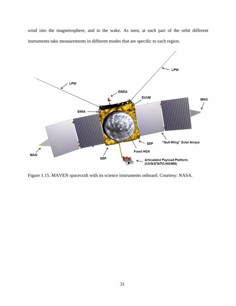
31

wind into the magnetosphere, and in the wake. As seen, at each part of the orbit different

instruments take measurements in different modes that are specific to each region.

Figure 1.15. MAVEN spacecraft with its science instruments onboard. Courtesy: NASA.

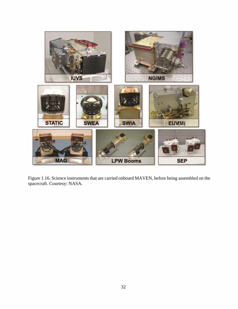
32

Figure 1.16. Science instruments that are carried onboard MAVEN, before being assembled on the

spacecraft. Courtesy: NASA.

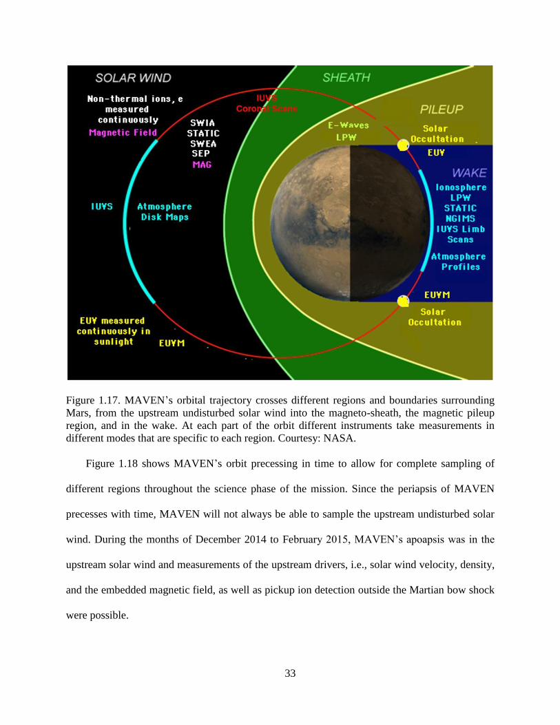
33

Figure 1.17. MAVEN’s orbital trajectory crosses different regions and boundaries surrounding

Mars, from the upstream undisturbed solar wind into the magneto-sheath, the magnetic pileup

region, and in the wake. At each part of the orbit different instruments take measurements in

different modes that are specific to each region. Courtesy: NASA.

Figure 1.18 shows MAVEN’s orbit precessing in time to allow for complete sampling of

different regions throughout the science phase of the mission. Since the periapsis of MAVEN

precesses with time, MAVEN will not always be able to sample the upstream undisturbed solar

wind. During the months of December 2014 to February 2015, MAVEN’s apoapsis was in the

upstream solar wind and measurements of the upstream drivers, i.e., solar wind velocity, density,

and the embedded magnetic field, as well as pickup ion detection outside the Martian bow shock

were possible.

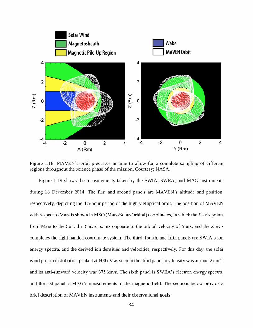
34

Figure 1.18. MAVEN’s orbit precesses in time to allow for a complete sampling of different

regions throughout the science phase of the mission. Courtesy: NASA.

Figure 1.19 shows the measurements taken by the SWIA, SWEA, and MAG instruments

during 16 December 2014. The first and second panels are MAVEN’s altitude and position,

respectively, depicting the 4.5-hour period of the highly elliptical orbit. The position of MAVEN

with respect to Mars is shown in MSO (Mars-Solar-Orbital) coordinates, in which the X axis points

from Mars to the Sun, the Y axis points opposite to the orbital velocity of Mars, and the Z axis

completes the right handed coordinate system. The third, fourth, and fifth panels are SWIA’s ion

energy spectra, and the derived ion densities and velocities, respectively. For this day, the solar

wind proton distribution peaked at 600 eV as seen in the third panel, its density was around 2 cm-3,

and its anti-sunward velocity was 375 km/s. The sixth panel is SWEA’s electron energy spectra,

and the last panel is MAG’s measurements of the magnetic field. The sections below provide a

brief description of MAVEN instruments and their observational goals.

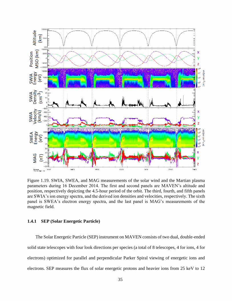
35

Figure 1.19. SWIA, SWEA, and MAG measurements of the solar wind and the Martian plasma

parameters during 16 December 2014. The first and second panels are MAVEN’s altitude and

position, respectively depicting the 4.5-hour period of the orbit. The third, fourth, and fifth panels

are SWIA’s ion energy spectra, and the derived ion densities and velocities, respectively. The sixth

panel is SWEA’s electron energy spectra, and the last panel is MAG’s measurements of the

magnetic field.

1.4.1 SEP (Solar Energetic Particle)

The Solar Energetic Particle (SEP) instrument on MAVEN consists of two dual, double-ended

solid state telescopes with four look directions per species (a total of 8 telescopes, 4 for ions, 4 for

electrons) optimized for parallel and perpendicular Parker Spiral viewing of energetic ions and

electrons. SEP measures the flux of solar energetic protons and heavier ions from 25 keV to 12

36

MeV and electrons from 25 keV to 1 MeV with a 30% energy resolution and a 2-second time

resolution. SEP can measure energy fluxes that range from 10 to 106 eV/[cm2 s sr eV] to

characterize solar energetic particles in an energy range that affects the upper atmosphere and

ionosphere of Mars through sputtering, heating, dissociation, excitation, and ionization. SEP has a

mechanical pinhole attenuator that protects against overheating when the Sun is in its field of view,

reduces count rates during periods of high flux, and reduces radiation damage caused by low

energy ions during periods of high flux [Larson et al., 2015].

SEP can also measure energetic pickup oxygen ions that are born in the distant exosphere of

Mars and energized by the motional electric field associated with the solar wind magnetic field.

These pickup ions are created due to ionization of the neutral oxygen atoms that are mainly

escaping from Mars [Rahmati et al., 2014,2015]. Therefore, SEP measurements of these pickup

ions, which are discussed in Chapter 4, can provide constraints on neutral oxygen escape from

Mars. The SEP instrument is described in more detail in Chapter 4 and pickup oxygen model-data

comparisons are provided.

1.4.2 SWIA (Solar Wind Ion Analyzer)

The Solar Wind Ion Analyzer (SWIA) instrument on MAVEN measures ion distributions in

the solar wind as well as the plasma environment of Mars from 25 eV to 25 keV with an energy

resolution of 10%, an angular resolution of 22.5°, and a time resolution of 4 seconds. It also

determines the solar wind proton and alpha particle angular distributions with an angular resolution

of 4.5°. Density and velocity measurements by SWIA determine the bulk plasma flow of the solar

wind (300 km/s to 1000 km/s) as well as the stagnated magneto-sheath speeds (tens of km/s) with

a density range of 0.1 cm-3 to 100 cm-3. Measurements of the solar wind and magnetosheath plasma

37

flow around Mars constrain the ionization rates of neutrals from charge exchange, a key input to

atmospheric loss processes. The nature of solar wind interaction with the upper atmosphere is an

important driver of atmospheric escape from Mars. SWIA helps determine the structure and

variability of the Martian magnetosheath, and characterizes processes such as reconnection, flux

ropes, bulk plasma escape, and auroral processes throughout the Martian system [Halekas et al.,

2013].

The SWIA measurements of the solar wind velocity are used in this work to calculate pickup

ion trajectories. Solar wind density measurements by SWIA are also used to calculate charge

exchange rates between solar wind protons and exospheric neutral hydrogen and oxygen atoms.

SWIA is also able to measure the low energy part of the pickup oxygen distribution [Rahmati et

al., 2014,2015] and the pickup ion measurements are modeled in this work. The SWIA instrument

is described in more detail in Chapter 4 and pickup ion model-data comparisons are provided.

1.4.3 SWEA (Solar Wind Electron Analyzer)

The Solar Wind Electron Analyzer (SWEA) instrument on MAVEN is a hemispherical

electrostatic analyzer with deflectors that measures electrons with energies from 5 eV to 4.6 keV

with an energy resolution of ΔE/E = 17% with capability for ΔE/E = 9% below 50 eV. SWEA

measures energy fluxes of electrons from 103 to 109 eV/[cm2 s sr eV] in a 360° × 120° (azimuth ×

elevation) field of view with an angular resolution of 22.5° × 20° and a time resolution of 2

seconds. The magnetic field topology at Mars can be deduced form SWEA measurements of

electron pitch angle distributions and loss cone; therefore, helping the MAG instrument in

constructing the magneto-plasma topology of Mars in and above the ionosphere. SWEA is

38

mounted at the end of a 1.5-meter boom to isolate it from residual spacecraft magnetic fields, as

well as spacecraft photoelectrons [Mitchell et al., 2015].

SWEA data help determine the primary ionospheric photoelectron spectrum at Mars and find

electron impact ionization rates in the Martian ionosphere and exosphere [Sakai et al., 2015]. The

measurements can also be used to determine auroral electron populations at Mars. In Chapter 3

and Chapter 4, the SWEA measurements are used to calculated electron impact ionization rates

for hydrogen and oxygen atoms in the undisturbed upstream solar wind.

1.4.4 MAG (Magnetometer)

Measuring the magnetic field in the plasma environment of Mars is very important, because

electrons and ions are bound to and gyrate about the magnetic field lines. Plasma trajectories are

dictated by the magnitude and direction of these field lines that originate from the Sun and are

carried by the solar wind. The interplanetary magnetic field is draped around Mars and is affected

by the Mars crustal magnetic fields, which are believed to be the remnants of the global magnetism

that once existed on Mars before the internal dynamo cooled down and turned off the global

magnetic field. These crustal magnetic fields act as mini-magnetospheres that affect the interaction

of the solar wind with Mars.

There are two ring core fluxgate magnetometer (MAG) instruments on MAVEN located at

the ends of each solar panel that measure the vector magnetic field in the unperturbed solar wind

(B = 1-20 nT), magnetosheath (B = 10-50 nT), and crustal fields (B < 3000 nT), with the ability to

spatially resolve crustal magnetic fields. The dynamic range of MAG is from 0.1 nT to 60,000 nT

with a 32 Hz time resolution, 1° angular determination of vector magnetic field, and 5% precision

39

on its scalar value [Connerney et al., 2015a,b]. The MAG measurements of the interplanetary

magnetic field are used in Chapter 4 to calculate trajectories of hydrogen and oxygen pickup ions

in the undisturbed upstream solar wind.

1.4.5 EUVM (Extreme UltraViolet Monitor)

The solar Extreme Ultraviolet (EUV) radiation is a driver of atmospheric escape by means of

ionizing and heating the upper atmosphere, as well as initiating the photochemistry in the

ionosphere of Mars. EUV photons with different wavelengths originate from different regions of

the outer layers of the Sun, i.e., photosphere, chromospheres, and corona. The intensity of the solar

irradiance varies on time scales of minutes to hours due to solar flares, days to months due to the

solar rotation, and years to decades due to the solar magnetic activity cycle. MAVEN arrived at

Mars just after the peak of the solar cycle 24 (solar maximum) and the sunspot number decreases

during the science phase of the mission. During the solar maximum cycle, the frequency of the

occurrence of solar flares tends to be the highest, making it possible for MAVEN to study the

response of the upper atmosphere of Mars to flares [Thiemann et al., 2015]. As the solar activity

decreases, MAVEN measurements of the solar irradiance variability can be used to relate the solar

photon flux input to the escape of volatiles at Mars.

The Extreme UltraViolet Monitor (EUVM) instrument on MAVEN measures the solar

irradiance variability at Mars for wavelengths that are responsible for ionization, dissociation, and

heating of the upper atmosphere of Mars. EUVM has three photometers sensitive to different parts

of the EUV spectrum, i.e., 0.1-7 nm, 17-22 nm, and 121.6 nm. The full EUV spectrum (0-200 nm)

is derived by the FISM (Flare Irradiance Spectral Model) from EUVM measurements, and used in

models of the upper atmosphere [Eparvier et al., 2015]. In Chapter 3 and Chapter 4, the FISM

40

derived spectra are used in calculating the photo-ionization rates of oxygen and hydrogen atoms

in the Martian exosphere, in order to find fluxes of pickup ions at Mars.

1.4.6 IUVS (Imaging UltraViolet Spectrograph)

The Imaging UltraViolet Spectrograph (IUVS) on MAVEN is a remote sensing instrument

that uses a two dimensional array of active pixel sensors to acquire imaging spectroscopy in UV

wavelengths. The Far Ultraviolet (FUV) channel works in 110-190 nm at 0.6 nm resolution, and

the Middle Ultraviolet (MUV) channel works in 180-340 nm at 1.2 nm resolution. The instrument

is mounted on the spacecraft’s Articulated Payload Platform (APP) to accommodate pointing

requirements. The vertical spatial resolution of acquired images is 6 km on the limb and the

horizontal resolution is 200 km [McClintock et al., 2014].

IUVS provides constraints on escape processes by measuring vertical profiles of neutrals and

ions through limb scans near each periapsis and carries out stellar occultation campaigns to

characterize the composition and structure of the upper atmosphere [Gröller et al., 2015]. The

density profiles and column abundances of H, C, N, O, CO, N2, and CO2 from the homopause to

two scale heights above the exobase will be derived from IUVS data [Evans et al., 2015; Stevens

et al., 2015]. IUVS measurements will also provide profiles and column densities of C+, CO+, and

CO2+ from the ionospheric main peak to 400-500 km. When MAVEN is near its apoapsis, IUVS

acquires global images and disc maps of Mars to characterize spatial distribution and variability

of volatiles as well as measure the FUV airglow and the MUV reflected sunlight from the ozone,

dust, and clouds at Mars. In order to determine hot oxygen density profiles and deuterium to

hydrogen ratios (D/H), the coronal scans taken by IUVS in each orbit are used [Deighan et al.,

2015; Chaffin et al., 2015, Jain et al., 2015; Chaufray et al., 2015b].

41

1.4.7 STATIC (Supra-Thermal and Thermal Ion Composition)

The Supra-Thermal and Thermal Ion Composition (STATIC) instrument on MAVEN is a

toroidal electrostatic analyzer that detects ions in the plasma environment of Mars with an energy

to charge ratio of 0.1 keV/e to 30 keV/e, a 15% energy resolution, and a 4 second time resolution.

It includes a time of flight capability to resolve ion masses in the range 1-70 amu (atomic mass

unit) with a mass resolution of 25%. STATIC measures the composition of thermal ions in the

ionosphere that are in the energy range 0.1-10 eV, as well as suprathermal and energetic tail ions

of 5-100 eV, and pickup ions with E > 100 eV up to 30 keV. Key ion measurements include H+,

O+, O2+, and CO2

+ in a 360° × 90° field of view with angular resolution of 22.5° × 6°, and energy

flux of 104 to 108 eV/[cm2 s sr eV] when the attenuators are off. STATIC includes 2 attenuators,

one mechanical and one electrostatic, that extend the energy flux dynamic range to 1012

eV/[cm2 s sr eV]. Measurements of STATIC can be used to determine processes that energize ions

on their way to escape from Mars, and find energy distributions and pitch angle variations of those

ions [McFadden et al., 2015].

1.4.8 LPW (Langmuir Probe and Waves)

The Langmuir Probe and Waves (LPW) instrument on MAVEN is designed to measure the in

situ electron and ion densities and temperatures from the ionospheric peak (120-150 km) up to the

nominal ionopause location (300-500 km). It also measures the electric field wave power, which

is important for determining ion wave heating processes. The measurements from LPW determine

the electron temperatures required for calculation of ion recombination rates and ionospheric

chemistry [Ergun et al., 2015]. The data from LPW help characterize the global structure,

variability, and thermal properties of the Martian ionosphere [Andrews et al., 2015]. Determining

42

the effects of solar wind generated plasma waves and auroral precipitation on ionosphere heating

and its relationship to plasma escape is one of the goals of the instrument. LPW can also detect

dust impacts on the spacecraft by measuring the plasma cloud created due to the high impact

velocity of dust particles relative to the spacecraft (tens of km/s) [Andersson et al., 2015b].

LPW consists of two cylindrical booms, each 7 meters in length. The current-voltage (I-V)

sweep sensor works in the range ±50 Volts with 128 voltage steps swept in 2 seconds. The I-V

sweep curves can be used to derive photoelectron currents as well as thermal electron densities in

the ionosphere from 100 cm-3 to 106 cm-3, and electron temperatures in the range 500 K to 5000

K. The range of current measurement is 0.2 mA, with a resolution of 3.1 nA. The range of electric

field measurement is ±1 V/m, with a resolution of 0.3 V/km. Low frequency electric field is

measured in the frequency range 0.05 Hz to 10 Hz, and high frequency electric field is measured

in the frequency range 90 kHz to 1.6 MHz. In addition to the passive electric field measurements,

LPW can also operate in active sounding mode by transmitting white noise and measuring the

stimulated plasma Langmuir waves in the 50 kHz to 1.6 MHz frequency range. The electric field

wave spectra are used to calibrate the plasma density measurements [Andersson et al., 2015a].

1.4.9 NGIMS (Neutral Gas and Ion Mass Spectrometer)

The Neutral Gas and Ion Mass Spectrometer (NGIMS) on MAVEN is a quadrupole mass

spectrometer with a closed source that measures non-wall-reactive neutrals, and an open source

that measures wall-reactive neutrals and ions in the mass range 2-150 Da (H2 to Xe), with a mass

resolution of 1 Da, a count dynamic range of 108 counts/sec, and a sensitivity of 10-2

(counts/sec)/(particles/cm-3). NGIMS is mounted on the APP and its open source points in the ram

direction during observations [Mahaffy et al., 2014].

43

For the first time after the Viking missions, the measurements from NGIMS reveal the

structure and variation of the Martian upper atmosphere for major neutral species (He, N, O, CO,

N2, NO, O2, Ar, and CO2) and their major isotopes as well as ionospheric densities (thermal O2+,

CO2+, NO+, O+, CO+, C+, N2

+, OH+, and N+). The neutrals will be measured from the homopause

(well-mixed lower atmosphere) to above the exobase (up to ~400 km) where escape occurs, and

the ions from the ionospheric main peak (~120 km) to 400-500 km. NGIMS measurements provide

a basis for the study of transport, circulation, and energetics of the Martian thermospheric, as well

as the formation of the ionosphere. Isotope ratios can be derived from the NGIMS data (13C/12C,

18O/16O, 15N/14N, 40Ar/36Ar, and 38Ar/36Ar) and will shed light on the history of volatile escape and

climate change on Mars. NGIMS data help refine atmospheric circulation and ionosphere models

for Mars [Mahaffy et al., 2014].

1.5 This Work

On Mars the hot oxygen exosphere extends to several Martian radii and at high altitudes most

of the oxygen atoms in the exosphere are escaping. Directly probing this extended exosphere is

very challenging due to the very low oxygen densities at high altitudes. For example, according to

Rahmati et al. [2014] the exospheric density of hot oxygen atoms at 10,000 km is ~100 cm-3 and

at 100,000 km is only ~1 cm-3. Neutral detectors carried by spacecraft are not sensitive enough to

measure such low densities in situ. Remote sensing detectors such as ultraviolet spectrographs also

do not have sufficient sensitivity to detect scattered light or emission lines from such low densities.

This work aims to provide evidence for the existence of the extended exosphere of Mars from

oxygen pickup ion measurements by MAVEN. In this work data from the SEP, SWIA, SWEA,

44

MAG, and EUVM instruments are used to analyze pickup ion fluxes upstream of the Martian bow

shock.

In Chapter 2 the production and transport of hot oxygen atoms as well as oxygen escape

probabilities and escape rates are discussed. The thermospheric and ionospheric density and

temperature profiles from the MTGCM are used in two different models of hot O production and

transport to construct the exospheric densities of hot oxygen atoms at Mars. A two-

stream/Liouville code and a Monte-Carlo code are utilized to calculate the flux and distribution of

hot O atoms, and escape fluxes are predicted for solar maximum and minimum conditions.

Chapter 3 describes the method used to calculate the pickup ion fluxes upstream of Mars in

the undisturbed and uniform solar wind fields. Equations of motion of pickup ions are analytically

solved and a few cases with different solar wind conditions are assumed and pickup ion

trajectories, distributions, and fluxes for each case are presented.

Chapter 4 provides the evidence for the extended exosphere of Mars by utilizing pickup ion

model-data comparisons to confirm the presence of photo-chemically produced escaping hot

oxygen atoms at very high altitudes at Mars. The conditions under which the SEP and SWIA

instruments on MAVEN are able to detect pickup oxygen ions are described and a few orbits are

analyzed during which each instrument detected pickup ions.

Chapter 5 concludes the work by explaining how model-data comparisons can be used to

constrain models of hot O production and transport and their associated escape rates. A preliminary

escape flux, escape rate, and the total amount of water removed from Mars by the photo-chemical

45

escape of oxygen is presented for solar moderate conditions as constrained by pickup ion model-

data comparisons.

46

2 The Hot Oxygen Exosphere of Mars

Mars possesses a very extensive exosphere, which resembles a comet’s neutral coma in

extending out to tens of thousands of kilometers. The exosphere of Mars is populated with thermal

hydrogen atoms from the tail of the Maxwell-Boltzmann distribution, as well as hot oxygen atoms

produced via photo-chemical processes in the ionosphere. Part of the hot oxygen atoms in the

Martian exosphere can overcome Mars’s gravity and escape into space. The extended exosphere

of Mars directly interacts with the solar wind via the pickup and mass loading processes, where

neutral atoms in the exosphere are ionized and picked up by the solar wind fields. The conservation

of momentum requires that the solar wind flow slows down and is deflected in this process, since

part of its momentum is taken away by oxygen and hydrogen pickup ions.

Directly observing the oxygen exosphere of Mars and measuring the oxygen escape rate is

difficult due to low densities. Therefore, in the past few decades, models of the transport of hot

oxygen atoms are utilized to calculate the escape flux of oxygen from Mars. Escape flux

calculations are carried out for different phases of the solar cycle and also for the day and night

sides of Mars. The amount of solar radiation varies over one solar cycle and affects the densities

and temperatures of planetary atmospheres. High solar activity escape rates at Mars are found to

be higher than those of low solar activity [Kim et al., 1998]. The day side of Mars is in direct

interaction with the solar wind and ultra-violet photons from the Sun, making it more abundant in

ions and electrons. Therefore, escape rates on the day side are also higher than those of the night

side.

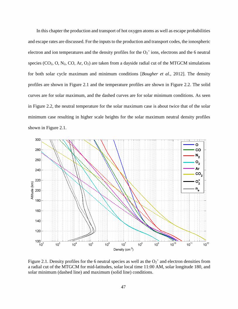
47

In this chapter the production and transport of hot oxygen atoms as well as escape probabilities

and escape rates are discussed. For the inputs to the production and transport codes, the ionospheric

electron and ion temperatures and the density profiles for the O2+ ions, electrons and the 6 neutral

species (CO2, O, N2, CO, Ar, O2) are taken from a dayside radial cut of the MTGCM simulations

for both solar cycle maximum and minimum conditions [Bougher et al., 2012]. The density

profiles are shown in Figure 2.1 and the temperature profiles are shown in Figure 2.2. The solid

curves are for solar maximum, and the dashed curves are for solar minimum conditions. As seen

in Figure 2.2, the neutral temperature for the solar maximum case is about twice that of the solar

minimum case resulting in higher scale heights for the solar maximum neutral density profiles

shown in Figure 2.1.

Figure 2.1. Density profiles for the 6 neutral species as well as the O2+ and electron densities from

a radial cut of the MTGCM for mid-latitudes, solar local time 11:00 AM, solar longitude 180, and

solar minimum (dashed line) and maximum (solid line) conditions.

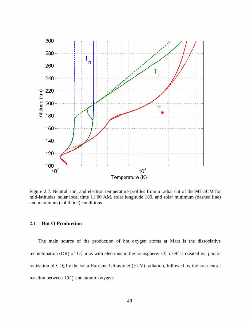
48

Figure 2.2. Neutral, ion, and electron temperature profiles from a radial cut of the MTGCM for

mid-latitudes, solar local time 11:00 AM, solar longitude 180, and solar minimum (dashed line)

and maximum (solid line) conditions.

2.1 Hot O Production

The main source of the production of hot oxygen atoms at Mars is the dissociative

recombination (DR) of

2O ions with electrons in the ionosphere.

2O itself is created via photo-

ionization of CO2 by the solar Extreme Ultraviolet (EUV) radiation, followed by the ion neutral

reaction between

2CO and atomic oxygen:

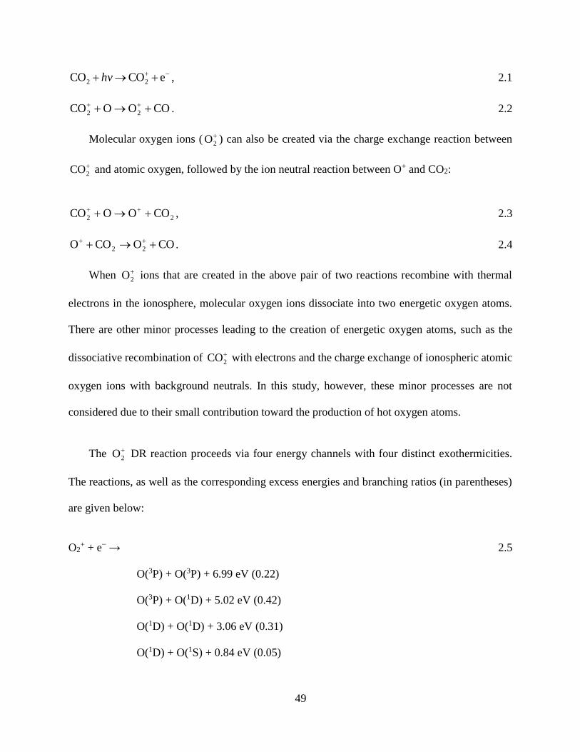
49

eCOCO 22 hv , 2.1

COOOCO 22 . 2.2

Molecular oxygen ions (

2O ) can also be created via the charge exchange reaction between

2CO and atomic oxygen, followed by the ion neutral reaction between O+ and CO2:

22 COOOCO , 2.3

COOCOO 22 . 2.4

When

2O ions that are created in the above pair of two reactions recombine with thermal

electrons in the ionosphere, molecular oxygen ions dissociate into two energetic oxygen atoms.

There are other minor processes leading to the creation of energetic oxygen atoms, such as the

dissociative recombination of

2CO with electrons and the charge exchange of ionospheric atomic

oxygen ions with background neutrals. In this study, however, these minor processes are not

considered due to their small contribution toward the production of hot oxygen atoms.

The

2O DR reaction proceeds via four energy channels with four distinct exothermicities.

The reactions, as well as the corresponding excess energies and branching ratios (in parentheses)

are given below:

O2+ + e− → 2.5

O(3P) + O(3P) + 6.99 eV (0.22)

O(3P) + O(1D) + 5.02 eV (0.42)

O(1D) + O(1D) + 3.06 eV (0.31)

O(1D) + O(1S) + 0.84 eV (0.05)

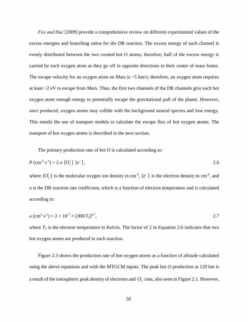
50

Fox and Hać [2009] provide a comprehensive review on different experimental values of the

excess energies and branching ratios for the DR reaction. The excess energy of each channel is

evenly distributed between the two created hot O atoms; therefore, half of the excess energy is

carried by each oxygen atom as they go off in opposite directions in their center of mass frame.

The escape velocity for an oxygen atom on Mars is ~5 km/s; therefore, an oxygen atom requires

at least ~2 eV to escape from Mars. Thus, the first two channels of the DR channels give each hot

oxygen atom enough energy to potentially escape the gravitational pull of the planet. However,

once produced, oxygen atoms may collide with the background neutral species and lose energy.

This entails the use of transport models to calculate the escape flux of hot oxygen atoms. The

transport of hot oxygen atoms is described in the next section.

The primary production rate of hot O is calculated according to:

P (cm-3 s-1) = 2 α ]O[ 2

][ e , 2.6

where ]O[ 2

is the molecular oxygen ion density in cm-3, ][ e is the electron density in cm-3, and

α is the DR reaction rate coefficient, which is a function of electron temperature and is calculated

according to:

α (cm3 s-1) = 2 × 10-7 × (300/Te)0.7, 2.7

where Te is the electron temperature in Kelvin. The factor of 2 in Equation 2.6 indicates that two

hot oxygen atoms are produced in each reaction.

Figure 2.3 shows the production rate of hot oxygen atoms as a function of altitude calculated

using the above equations and with the MTGCM inputs. The peak hot O production at 120 km is

a result of the ionospheric peak density of electrons and

2O ions, also seen in Figure 2.1. However,

51

at such low altitudes where the ionospheric peak is located, due to the high rate of collisions with

background neutrals, almost all of the produced hot O atoms lose their energy and become

thermalized. Modeling results explained in the following sections suggest that hot O atoms created

near the Martian exobase (~200 km) have the most contribution toward the escape of oxygen.

Figure 2.3. Production rate of hot oxygen atoms as a function of altitude for solar maximum (solid

line) and minimum (dashed line) conditions with temperature and density inputs from the

MTGCM.

Once the primary production of hot O is found, the branching ratios of the four energy

channels of the DR reaction are used to find the energy distribution of nascent hot O atoms. Since

electrons and molecular oxygen ions have non-zero temperatures before the dissociative

recombination process, the resulting hot O atoms will have a broadening in energy, especially in

high altitudes where electron and ion temperatures are higher. Figure 2.4 shows the production

rate of hot O atoms as a function of altitude and nascent energy for solar maximum conditions.

52

The four energy peaks correspond to the four channels of the

2O DR reaction. The energy spread

is found based on the Fox and Hać [1997] calculations of the spread in the nascent energy of hot

O atoms. Figure 2.5 is similar to Figure 2.4, but for solar minimum condition inputs. As seen, there

is less production for solar minimum compared to solar maximum conditions, due to lower plasma

densities at solar minimum.

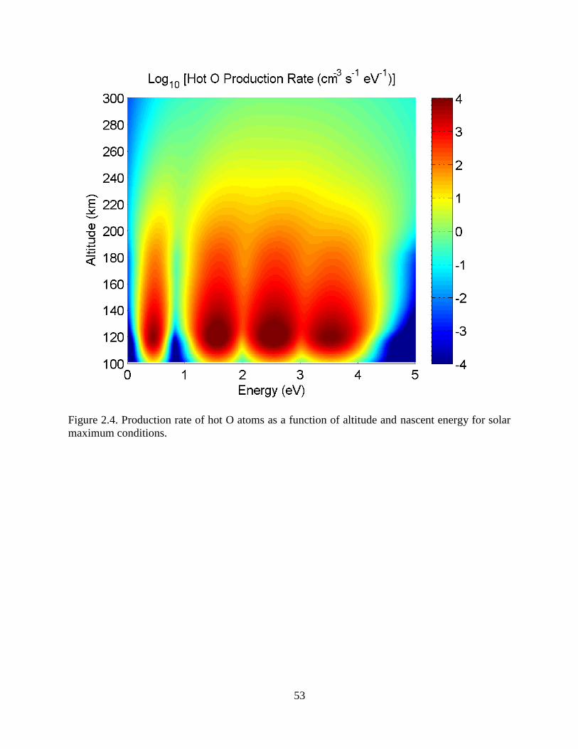
53

Figure 2.4. Production rate of hot O atoms as a function of altitude and nascent energy for solar

maximum conditions.

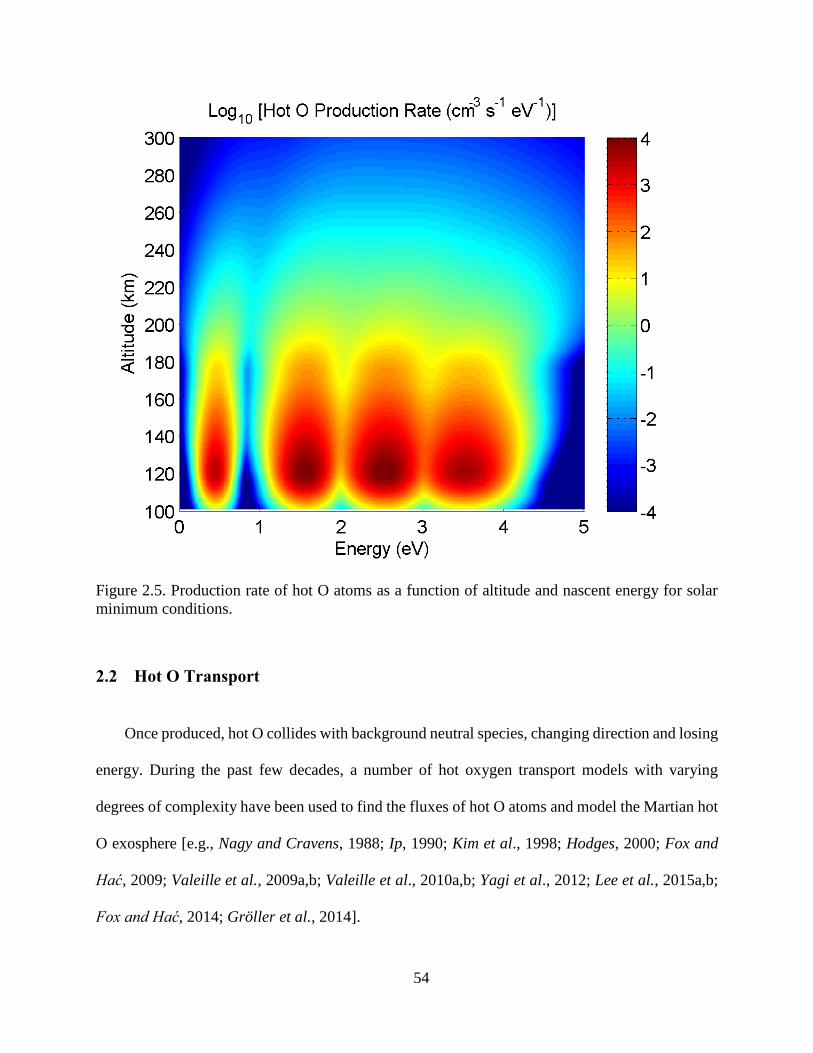
54

Figure 2.5. Production rate of hot O atoms as a function of altitude and nascent energy for solar

minimum conditions.

2.2 Hot O Transport

Once produced, hot O collides with background neutral species, changing direction and losing

energy. During the past few decades, a number of hot oxygen transport models with varying

degrees of complexity have been used to find the fluxes of hot O atoms and model the Martian hot

O exosphere [e.g., Nagy and Cravens, 1988; Ip, 1990; Kim et al., 1998; Hodges, 2000; Fox and

Hać, 2009; Valeille et al., 2009a,b; Valeille et al., 2010a,b; Yagi et al., 2012; Lee et al., 2015a,b;

Fox and Hać, 2014; Gröller et al., 2014].

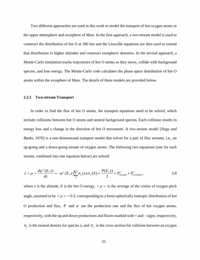
55

Two different approaches are used in this work to model the transport of hot oxygen atoms in

the upper atmosphere and exosphere of Mars. In the first approach, a two-stream model is used to

construct the distribution of hot O at 300 km and the Liouville equations are then used to extend

that distribution to higher altitudes and construct exospheric densities. In the second approach, a

Monte-Carlo simulation tracks trajectories of hot O atoms as they move, collide with background

species, and lose energy. The Monte-Carlo code calculates the phase space distribution of hot O

atoms within the exosphere of Mars. The details of these models are provided below.

2.2.1 Two-stream Transport

In order to find the flux of hot O atoms, the transport equations need to be solved, which

include collisions between hot O atoms and neutral background species. Each collision results in

energy loss and a change in the direction of hot O movement. A two-stream model [Nagy and

Banks, 1970] is a one-dimensional transport model that solves for a pair of flux streams, i.e., an

up-going and a down-going stream of oxygen atoms. The following two equations (one for each

stream, combined into one equation below) are solved:

secondarycascade2

),()( )(),(

),(PP

zEPEznzE

dz

zEds

s

s

, 2.8

where z is the altitude, E is the hot O energy, is the average of the cosine of oxygen pitch

angle, assumed to be = 0.5, corresponding to a hemi-spherically isotropic distribution of hot

O production and flux, P and are the production rate and the flux of hot oxygen atoms,

respectively, with the up and down productions and fluxes marked with + and – signs, respectively,

sn is the neutral density for species s, and s is the cross section for collision between an oxygen

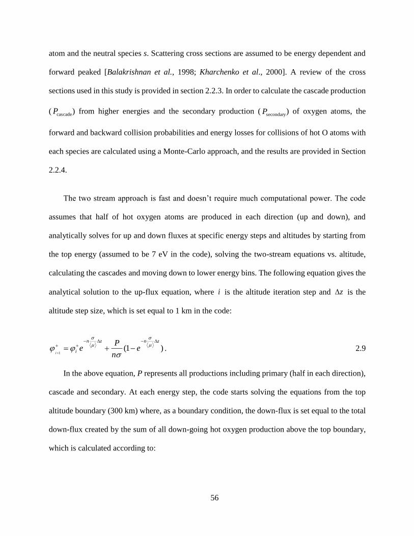
56

atom and the neutral species s. Scattering cross sections are assumed to be energy dependent and

forward peaked [Balakrishnan et al., 1998; Kharchenko et al., 2000]. A review of the cross

sections used in this study is provided in section 2.2.3. In order to calculate the cascade production

( cascadeP ) from higher energies and the secondary production (secondaryP ) of oxygen atoms, the

forward and backward collision probabilities and energy losses for collisions of hot O atoms with

each species are calculated using a Monte-Carlo approach, and the results are provided in Section

2.2.4.

The two stream approach is fast and doesn’t require much computational power. The code

assumes that half of hot oxygen atoms are produced in each direction (up and down), and

analytically solves for up and down fluxes at specific energy steps and altitudes by starting from

the top energy (assumed to be 7 eV in the code), solving the two-stream equations vs. altitude,

calculating the cascades and moving down to lower energy bins. The following equation gives the

analytical solution to the up-flux equation, where i is the altitude iteration step and z is the

altitude step size, which is set equal to 1 km in the code:

)1(1

znzn

i en

Pe

i

. 2.9

In the above equation, P represents all productions including primary (half in each direction),

cascade and secondary. At each energy step, the code starts solving the equations from the top

altitude boundary (300 km) where, as a boundary condition, the down-flux is set equal to the total

down-flux created by the sum of all down-going hot oxygen production above the top boundary,

which is calculated according to:

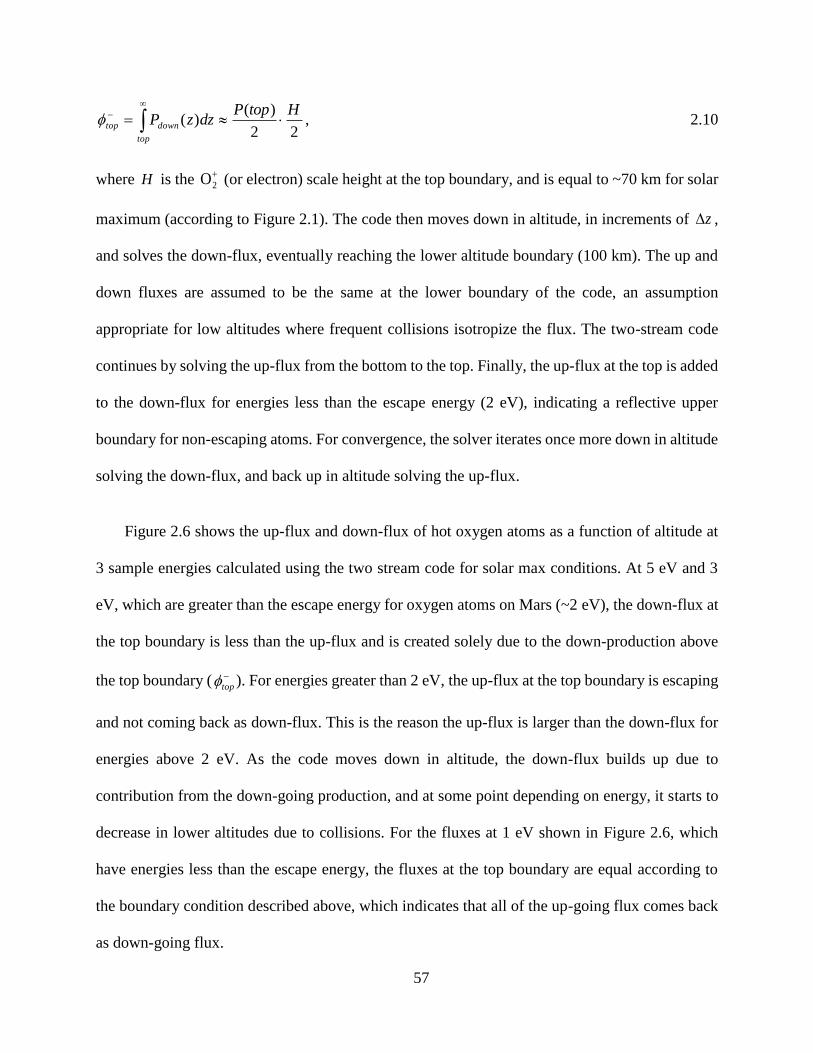
57

22

)()(

HtopPdzzP

top

downtop

, 2.10

where H is the

2O (or electron) scale height at the top boundary, and is equal to ~70 km for solar

maximum (according to Figure 2.1). The code then moves down in altitude, in increments of z ,

and solves the down-flux, eventually reaching the lower altitude boundary (100 km). The up and

down fluxes are assumed to be the same at the lower boundary of the code, an assumption

appropriate for low altitudes where frequent collisions isotropize the flux. The two-stream code

continues by solving the up-flux from the bottom to the top. Finally, the up-flux at the top is added

to the down-flux for energies less than the escape energy (2 eV), indicating a reflective upper

boundary for non-escaping atoms. For convergence, the solver iterates once more down in altitude

solving the down-flux, and back up in altitude solving the up-flux.

Figure 2.6 shows the up-flux and down-flux of hot oxygen atoms as a function of altitude at

3 sample energies calculated using the two stream code for solar max conditions. At 5 eV and 3

eV, which are greater than the escape energy for oxygen atoms on Mars (~2 eV), the down-flux at

the top boundary is less than the up-flux and is created solely due to the down-production above

the top boundary (

top ). For energies greater than 2 eV, the up-flux at the top boundary is escaping

and not coming back as down-flux. This is the reason the up-flux is larger than the down-flux for

energies above 2 eV. As the code moves down in altitude, the down-flux builds up due to

contribution from the down-going production, and at some point depending on energy, it starts to

decrease in lower altitudes due to collisions. For the fluxes at 1 eV shown in Figure 2.6, which

have energies less than the escape energy, the fluxes at the top boundary are equal according to

the boundary condition described above, which indicates that all of the up-going flux comes back

as down-going flux.

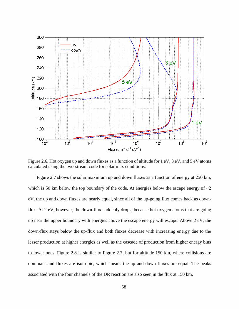
58

Figure 2.6. Hot oxygen up and down fluxes as a function of altitude for 1 eV, 3 eV, and 5 eV atoms

calculated using the two-stream code for solar max conditions.

Figure 2.7 shows the solar maximum up and down fluxes as a function of energy at 250 km,

which is 50 km below the top boundary of the code. At energies below the escape energy of ~2

eV, the up and down fluxes are nearly equal, since all of the up-going flux comes back as down-

flux. At 2 eV, however, the down-flux suddenly drops, because hot oxygen atoms that are going

up near the upper boundary with energies above the escape energy will escape. Above 2 eV, the

down-flux stays below the up-flux and both fluxes decrease with increasing energy due to the

lesser production at higher energies as well as the cascade of production from higher energy bins

to lower ones. Figure 2.8 is similar to Figure 2.7, but for altitude 150 km, where collisions are

dominant and fluxes are isotropic, which means the up and down fluxes are equal. The peaks

associated with the four channels of the DR reaction are also seen in the flux at 150 km.

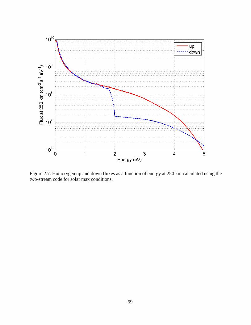
59

Figure 2.7. Hot oxygen up and down fluxes as a function of energy at 250 km calculated using the

two-stream code for solar max conditions.

60

Figure 2.8. Hot oxygen up and down fluxes as a function of energy at 150 km calculated using the

two-stream code for solar max conditions.

Figure 2.9 and Figure 2.10 show the up and down fluxes, respectively, versus energy and

altitude for solar max conditions. A general trend is seen in the up-flux figure where the flux

decreases with increasing energy. This is to be expected, since cascade in energy increases the flux

at lower energies. In the down-flux figure, the jump in the flux at the escape energy is distinct for

altitudes above ~220 km; however, below this altitude, collisions tend to smooth out the

discontinuity in the down-flux at the escape energy. By moving down in altitude from the top

boundary, the down-flux increases due to the down-going production from above and the back-

scattering of the up-flux coming from below. At some point in altitude the down-flux reaches its

maximum and then decreases due to collisions in lower altitudes.

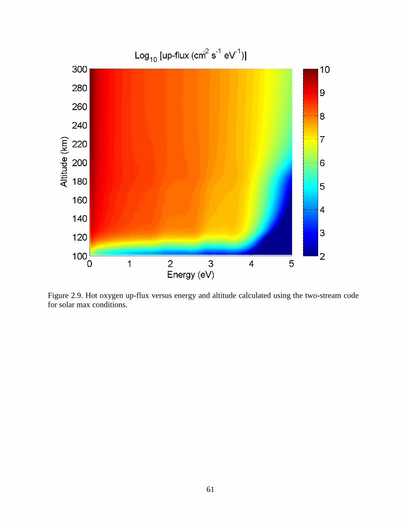
61

Figure 2.9. Hot oxygen up-flux versus energy and altitude calculated using the two-stream code

for solar max conditions.

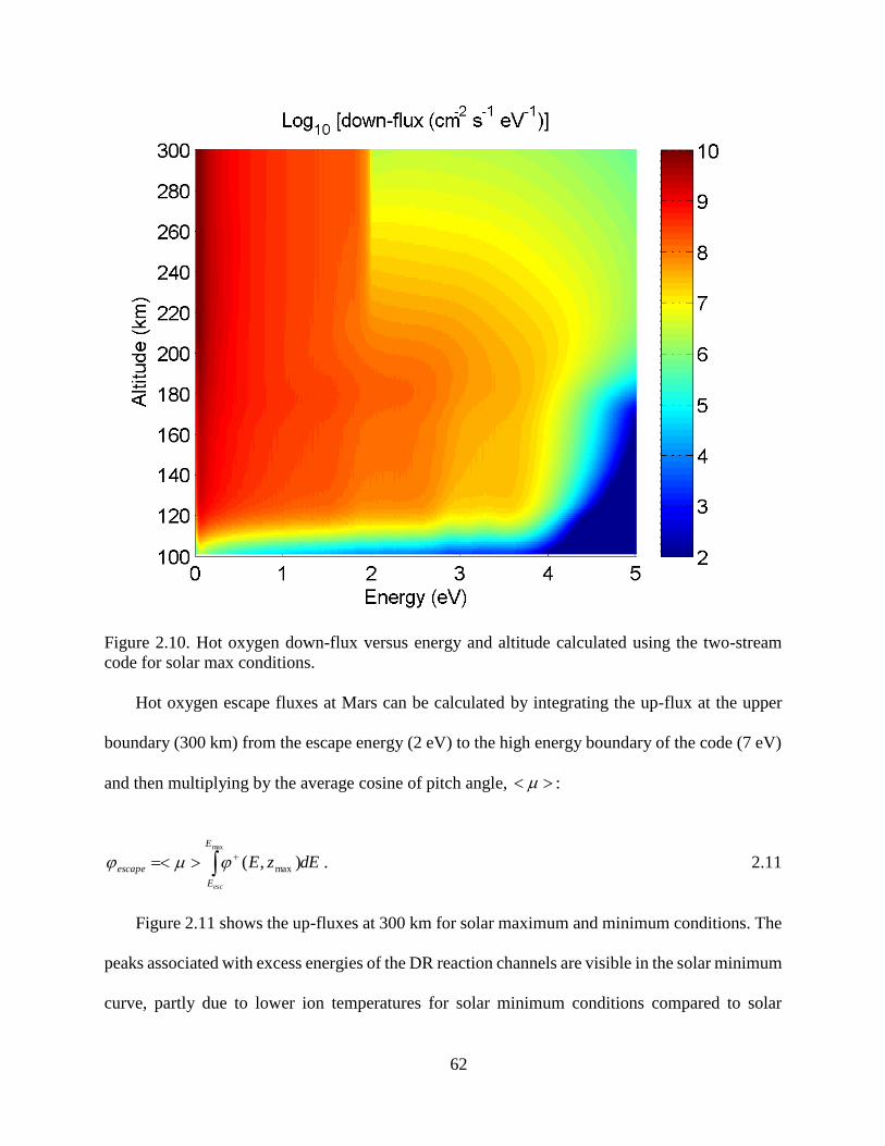
62

Figure 2.10. Hot oxygen down-flux versus energy and altitude calculated using the two-stream

code for solar max conditions.

Hot oxygen escape fluxes at Mars can be calculated by integrating the up-flux at the upper

boundary (300 km) from the escape energy (2 eV) to the high energy boundary of the code (7 eV)

and then multiplying by the average cosine of pitch angle, :

dEzE

E

E

escape

esc

max

),( max . 2.11

Figure 2.11 shows the up-fluxes at 300 km for solar maximum and minimum conditions. The

peaks associated with excess energies of the DR reaction channels are visible in the solar minimum

curve, partly due to lower ion temperatures for solar minimum conditions compared to solar

63

maximum, which narrows the spread in the nascent hot O energy, and partly due to lower

background neutral densities, which lowers the collision rates and prevents smoothing of the fluxes

in energy. Integrating the up-flux for both curves for energies above the escape energy and

multiplying by to get the escape flux gives hot oxygen escape fluxes of 9 × 107 cm-2 s-1 for

solar maximum and 4 × 107 cm-2 s-1 for solar minimum conditions.

Once the up and down fluxes are found by the two-stream code, the hot O energy distribution

function at the upper boundary of the code (300 km) is calculated according to the following

equation:

f (E) = ( φ+(E,zmax) + φ−(E,zmax) ) / v(E), 2.12

where v(E) is the velocity of hot O atoms with energy E. This energy distribution function can then

be fed into a Liouville code to find the hot O number densities in the Martian exosphere extending

out to several Martian radii (RM). Figure 2.12 shows the energy distribution of hot O atoms at 300

km for solar maximum and solar minimum conditions. The jump at 2 eV is due to the reflecting

boundary condition imposed at the top boundary for energies below the escape energy.

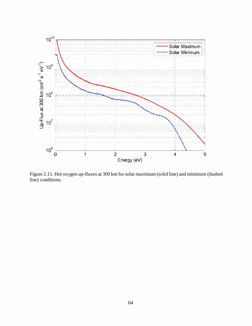
64

Figure 2.11. Hot oxygen up-fluxes at 300 km for solar maximum (solid line) and minimum (dashed

line) conditions.

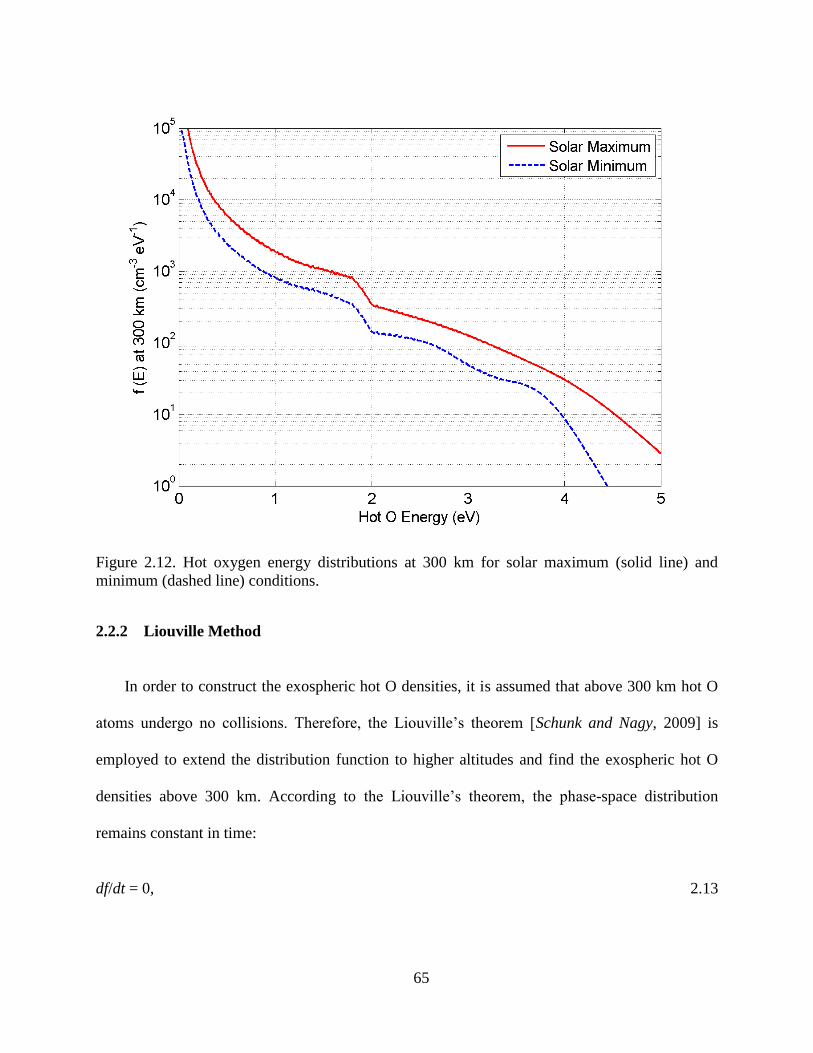
65

Figure 2.12. Hot oxygen energy distributions at 300 km for solar maximum (solid line) and

minimum (dashed line) conditions.

2.2.2 Liouville Method

In order to construct the exospheric hot O densities, it is assumed that above 300 km hot O

atoms undergo no collisions. Therefore, the Liouville’s theorem [Schunk and Nagy, 2009] is

employed to extend the distribution function to higher altitudes and find the exospheric hot O

densities above 300 km. According to the Liouville’s theorem, the phase-space distribution

remains constant in time:

df/dt = 0, 2.13

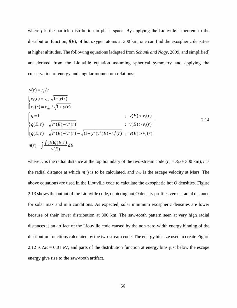
66

where f is the particle distribution in phase-space. By applying the Liouville’s theorem to the

distribution function, f(E), of hot oxygen atoms at 300 km, one can find the exospheric densities

at higher altitudes. The following equations [adapted from Schunk and Nagy, 2009, and simplified]

are derived from the Liouville equation assuming spherical symmetry and applying the

conservation of energy and angular momentum relations:

dEEv

rEqEfrn

rvEvrvEvyrvEvrEq

rvEvrvEvrEq

rvEvq

ryvrv

ryvrv

rrry

esc

esc

c

)(

),()()(

)()( ; )()()1( )()(),(

)()( ; )()(),(

)()( ; 0

)(1/)(

)(1)(

/)(

2

2

1

222

1

2

1

2

1

2

1

2

1

, 2.14

where rc is the radial distance at the top boundary of the two-stream code (rc = RM + 300 km), r is

the radial distance at which n(r) is to be calculated, and vesc is the escape velocity at Mars. The

above equations are used in the Liouville code to calculate the exospheric hot O densities. Figure

2.13 shows the output of the Liouville code, depicting hot O density profiles versus radial distance

for solar max and min conditions. As expected, solar minimum exospheric densities are lower

because of their lower distribution at 300 km. The saw-tooth pattern seen at very high radial

distances is an artifact of the Liouville code caused by the non-zero-width energy binning of the

distribution functions calculated by the two-stream code. The energy bin size used to create Figure

2.12 is ΔE = 0.01 eV, and parts of the distribution function at energy bins just below the escape

energy give rise to the saw-tooth artifact.

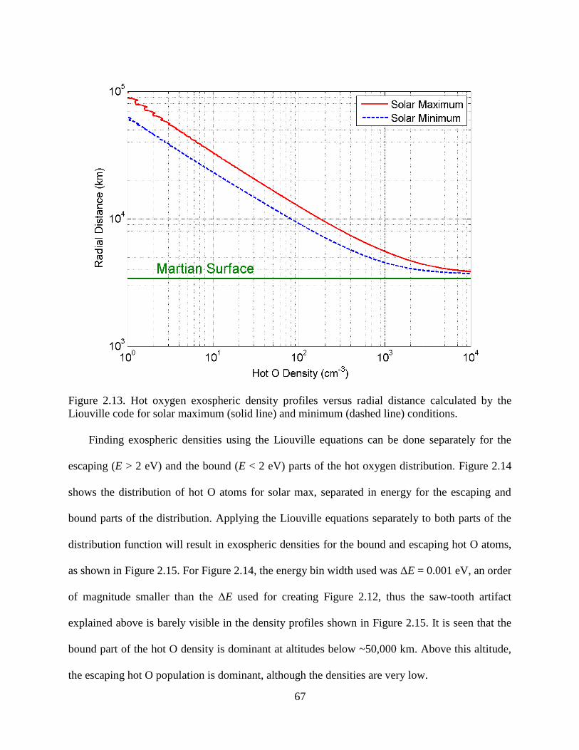
67


Liouville code for solar maximum (solid line) and minimum (dashed line) conditions.

Finding exospheric densities using the Liouville equations can be done separately for the

escaping (E > 2 eV) and the bound (E < 2 eV) parts of the hot oxygen distribution. Figure 2.14

shows the distribution of hot O atoms for solar max, separated in energy for the escaping and

bound parts of the distribution. Applying the Liouville equations separately to both parts of the

distribution function will result in exospheric densities for the bound and escaping hot O atoms,

as shown in Figure 2.15. For Figure 2.14, the energy bin width used was ΔE = 0.001 eV, an order

of magnitude smaller than the ΔE used for creating Figure 2.12, thus the saw-tooth artifact

explained above is barely visible in the density profiles shown in Figure 2.15. It is seen that the

bound part of the hot O density is dominant at altitudes below ~50,000 km. Above this altitude,

the escaping hot O population is dominant, although the densities are very low.

68

Figure 2.14. Hot oxygen energy distributions at 300 km for solar maximum conditions, separated

in energy for the escaping and bound parts of the distribution. Adapted from Figure 2 of Rahmati

et al. [2014].

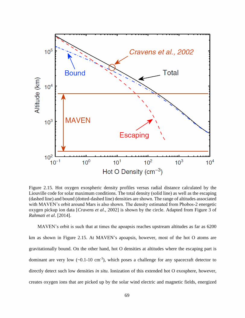
69


Liouville code for solar maximum conditions. The total density (solid line) as well as the escaping

(dashed line) and bound (dotted-dashed line) densities are shown. The range of altitudes associated

with MAVEN’s orbit around Mars is also shown. The density estimated from Phobos-2 energetic

oxygen pickup ion data [Cravens et al., 2002] is shown by the circle. Adapted from Figure 3 of

Rahmati et al. [2014].

MAVEN’s orbit is such that at times the apoapsis reaches upstream altitudes as far as 6200

km as shown in Figure 2.15. At MAVEN’s apoapsis, however, most of the hot O atoms are

gravitationally bound. On the other hand, hot O densities at altitudes where the escaping part is

dominant are very low (~0.1-10 cm-3), which poses a challenge for any spacecraft detector to

directly detect such low densities in situ. Ionization of this extended hot O exosphere, however,

creates oxygen ions that are picked up by the solar wind electric and magnetic fields, energized

70

and transported downstream towards Mars. Particle detectors on MAVEN (SEP, SWIA, STATIC)

can easily measure these energetic pickup ions and provide constraints on exospheric hot O

densities and escape rates. Cravens et al. [2002] used a similar method by analyzing the Phobos-

2 energetic pickup oxygen ion data to estimate the hot O density at ~10 RM. That estimate is also

shown by the circle in Figure 2.15.

2.2.3 Collision Cross Sections

In solving the two-stream equations and finding the cascade and secondary productions of hot

oxygen atoms, some information is required on scattering cross sections for collisions of oxygen

atoms with each background species. The total cross section values used in this work are adapted

from Fox and Hać [2014]. These cross sections are assumed to be energy dependent and have a

peak at forward scattering angles. The dependences on scattering angle and energy are assumed to

be the same for all species and adapted from Kharchenko et al. [2000] quantum mechanical

calculations of O-O collisions. The total cross sections for oxygen atoms colliding with each

background species with 3 eV relative energy are presented in Table 1. Also included are the

forward and backscatter probabilities and energy losses calculated using a Monte-Carlo approach,

which is described in the next section. Note that CO and N2 have the same mass; hence their

respective values in Table 1 are the same.

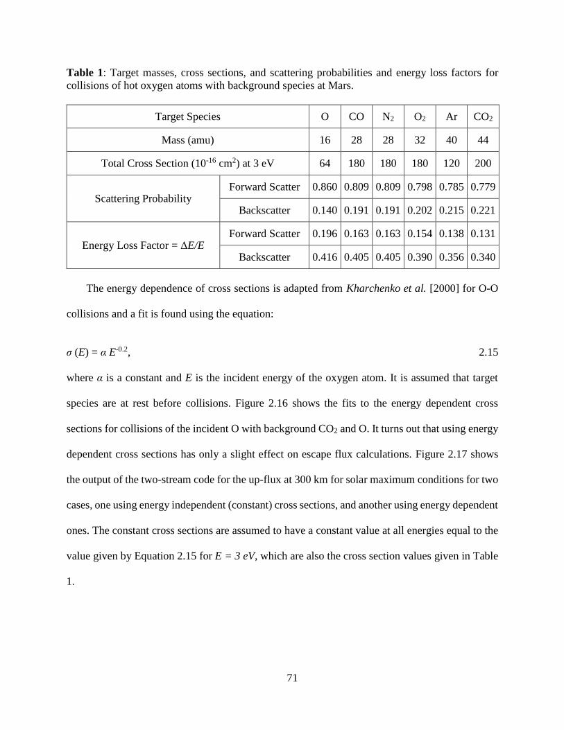
71

Table 1: Target masses, cross sections, and scattering probabilities and energy loss factors for

collisions of hot oxygen atoms with background species at Mars.

Target Species O CO N2 O2 Ar CO2

Mass (amu) 16 28 28 32 40 44

Total Cross Section (10-16 cm2) at 3 eV 64 180 180 180 120 200

Scattering Probability Forward Scatter 0.860 0.809 0.809 0.798 0.785 0.779

Backscatter 0.140 0.191 0.191 0.202 0.215 0.221

Energy Loss Factor = ΔE/E Forward Scatter 0.196 0.163 0.163 0.154 0.138 0.131

Backscatter 0.416 0.405 0.405 0.390 0.356 0.340

The energy dependence of cross sections is adapted from Kharchenko et al. [2000] for O-O

collisions and a fit is found using the equation:

σ (E) = α E-0.2, 2.15

where α is a constant and E is the incident energy of the oxygen atom. It is assumed that target

species are at rest before collisions. Figure 2.16 shows the fits to the energy dependent cross

sections for collisions of the incident O with background CO2 and O. It turns out that using energy

dependent cross sections has only a slight effect on escape flux calculations. Figure 2.17 shows

the output of the two-stream code for the up-flux at 300 km for solar maximum conditions for two

cases, one using energy independent (constant) cross sections, and another using energy dependent

ones. The constant cross sections are assumed to have a constant value at all energies equal to the

value given by Equation 2.15 for E = 3 eV, which are also the cross section values given in Table

1.

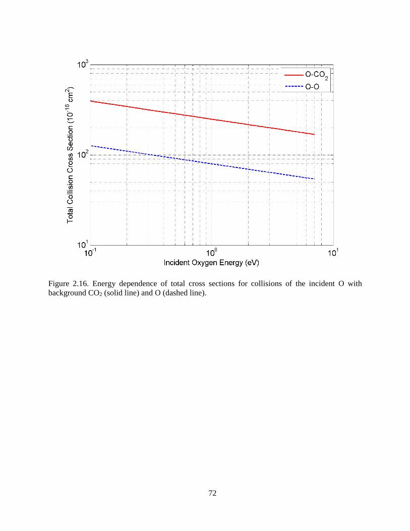
72

Figure 2.16. Energy dependence of total cross sections for collisions of the incident O with

background CO2 (solid line) and O (dashed line).

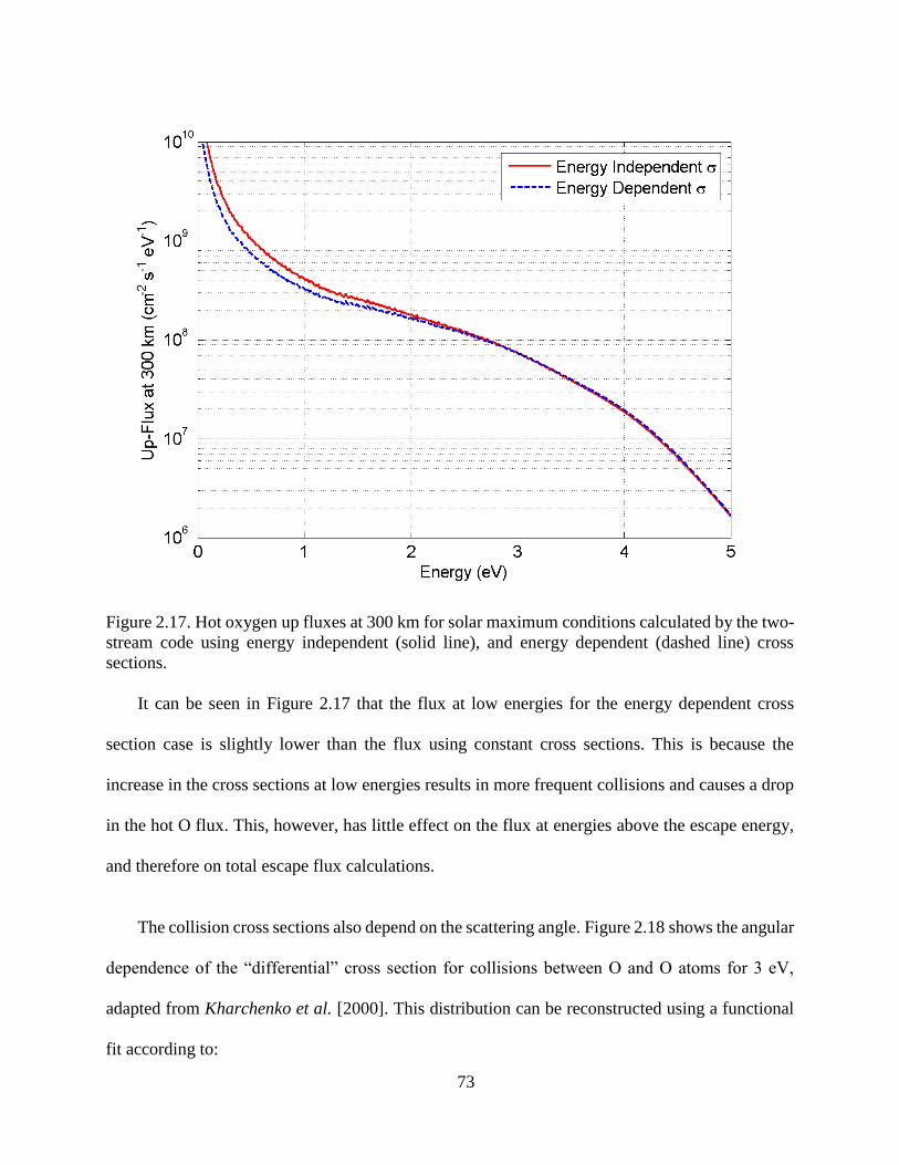
73

Figure 2.17. Hot oxygen up fluxes at 300 km for solar maximum conditions calculated by the two-

stream code using energy independent (solid line), and energy dependent (dashed line) cross

sections.

It can be seen in Figure 2.17 that the flux at low energies for the energy dependent cross

section case is slightly lower than the flux using constant cross sections. This is because the

increase in the cross sections at low energies results in more frequent collisions and causes a drop

in the hot O flux. This, however, has little effect on the flux at energies above the escape energy,

and therefore on total escape flux calculations.

The collision cross sections also depend on the scattering angle. Figure 2.18 shows the angular

dependence of the “differential” cross section for collisions between O and O atoms for 3 eV,

adapted from Kharchenko et al. [2000]. This distribution can be reconstructed using a functional

fit according to:

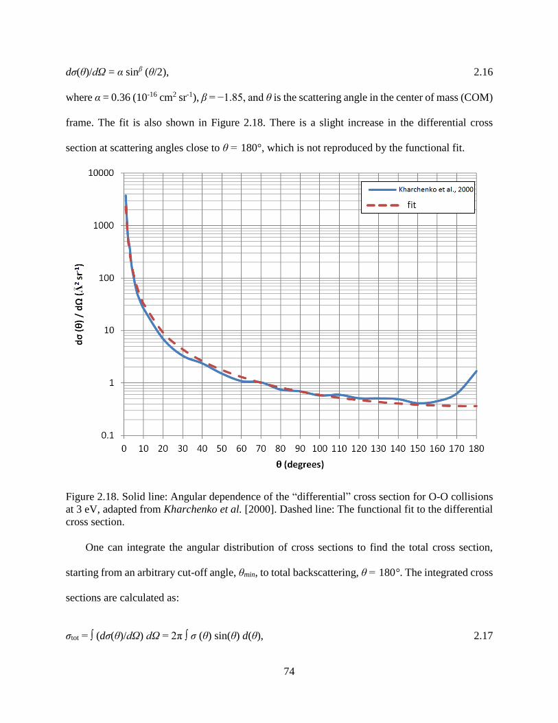
74

dσ(θ)/dΩ = α sinβ (θ/2), 2.16

where α = 0.36 (10-16 cm2 sr-1), β = −1.85, and θ is the scattering angle in the center of mass (COM)

frame. The fit is also shown in Figure 2.18. There is a slight increase in the differential cross

section at scattering angles close to θ = 180°, which is not reproduced by the functional fit.

Figure 2.18. Solid line: Angular dependence of the “differential” cross section for O-O collisions

at 3 eV, adapted from Kharchenko et al. [2000]. Dashed line: The functional fit to the differential

cross section.

One can integrate the angular distribution of cross sections to find the total cross section,

starting from an arbitrary cut-off angle, θmin, to total backscattering, θ = 180°. The integrated cross

sections are calculated as:

σtot = ∫ (dσ(θ)/dΩ) dΩ = 2π ∫ σ (θ) sin(θ) d(θ), 2.17

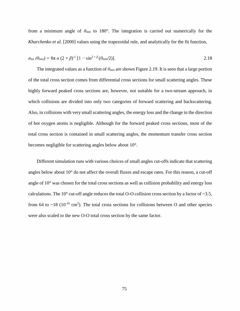
75

from a minimum angle of θmin to 180°. The integration is carried out numerically for the

Kharchenko et al. [2000] values using the trapezoidal rule, and analytically for the fit function,

σtot (θmin) = 8π α (2 + β)-1 [1 − sin2 + β (θmin/2)]. 2.18

The integrated values as a function of θmin are shown Figure 2.19. It is seen that a large portion

of the total cross section comes from differential cross sections for small scattering angles. These

highly forward peaked cross sections are, however, not suitable for a two-stream approach, in

which collisions are divided into only two categories of forward scattering and backscattering.

Also, in collisions with very small scattering angles, the energy loss and the change in the direction

of hot oxygen atoms is negligible. Although for the forward peaked cross sections, most of the

total cross section is contained in small scattering angles, the momentum transfer cross section

becomes negligible for scattering angles below about 10°.

Different simulation runs with various choices of small angles cut-offs indicate that scattering

angles below about 10° do not affect the overall fluxes and escape rates. For this reason, a cut-off

angle of 10° was chosen for the total cross sections as well as collision probability and energy loss

calculations. The 10° cut-off angle reduces the total O-O collision cross section by a factor of ~3.5,

from 64 to ~18 (10-16 cm2). The total cross sections for collisions between O and other species

were also scaled to the new O-O total cross section by the same factor.

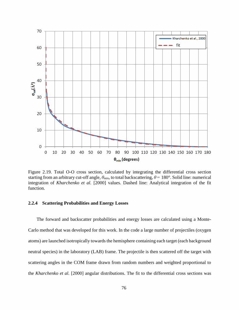
76

Figure 2.19. Total O-O cross section, calculated by integrating the differential cross section

starting from an arbitrary cut-off angle, θmin, to total backscattering, θ = 180°. Solid line: numerical

integration of Kharchenko et al. [2000] values. Dashed line: Analytical integration of the fit

function.

2.2.4 Scattering Probabilities and Energy Losses

The forward and backscatter probabilities and energy losses are calculated using a Monte-

Carlo method that was developed for this work. In the code a large number of projectiles (oxygen

atoms) are launched isotropically towards the hemisphere containing each target (each background

neutral species) in the laboratory (LAB) frame. The projectile is then scattered off the target with

scattering angles in the COM frame drawn from random numbers and weighted proportional to

the Kharchenko et al. [2000] angular distributions. The fit to the differential cross sections was

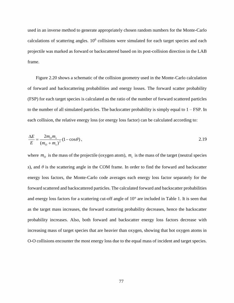
77

used in an inverse method to generate appropriately chosen random numbers for the Monte-Carlo

calculations of scattering angles. 106 collisions were simulated for each target species and each

projectile was marked as forward or backscattered based on its post-collision direction in the LAB

frame.

Figure 2.20 shows a schematic of the collision geometry used in the Monte-Carlo calculation

of forward and backscattering probabilities and energy losses. The forward scatter probability

(FSP) for each target species is calculated as the ratio of the number of forward scattered particles

to the number of all simulated particles. The backscatter probability is simply equal to 1 – FSP. In

each collision, the relative energy loss (or energy loss factor) can be calculated according to:

)cos1()(

22

sO

sO

mm

mm

E

E, 2.19

where Om is the mass of the projectile (oxygen atom), sm is the mass of the target (neutral species

s), and θ is the scattering angle in the COM frame. In order to find the forward and backscatter

energy loss factors, the Monte-Carlo code averages each energy loss factor separately for the

forward scattered and backscattered particles. The calculated forward and backscatter probabilities

and energy loss factors for a scattering cut-off angle of 10° are included in Table 1. It is seen that

as the target mass increases, the forward scattering probability decreases, hence the backscatter

probability increases. Also, both forward and backscatter energy loss factors decrease with

increasing mass of target species that are heavier than oxygen, showing that hot oxygen atoms in

O-O collisions encounter the most energy loss due to the equal mass of incident and target species.

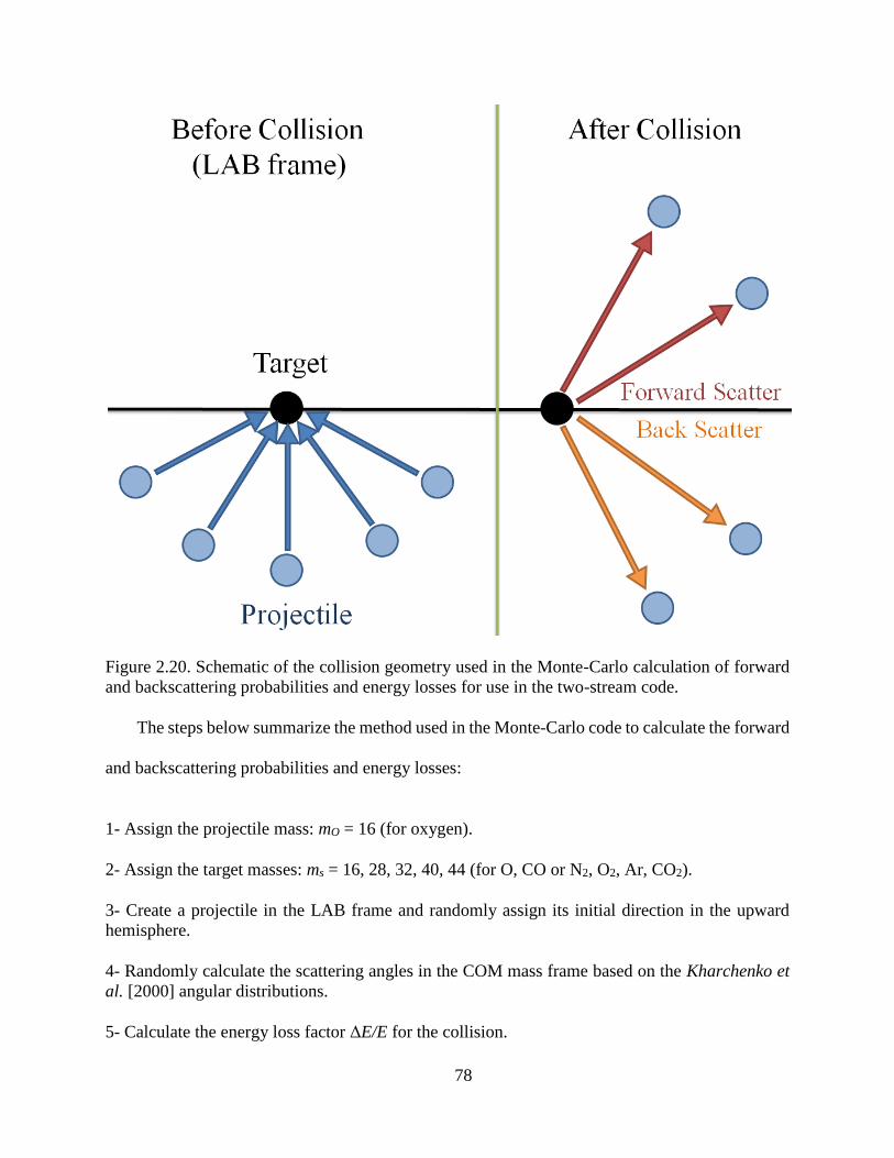
78

Figure 2.20. Schematic of the collision geometry used in the Monte-Carlo calculation of forward

and backscattering probabilities and energy losses for use in the two-stream code.

The steps below summarize the method used in the Monte-Carlo code to calculate the forward

and backscattering probabilities and energy losses:

1- Assign the projectile mass: mO = 16 (for oxygen).

2- Assign the target masses: ms = 16, 28, 32, 40, 44 (for O, CO or N2, O2, Ar, CO2).

3- Create a projectile in the LAB frame and randomly assign its initial direction in the upward

hemisphere.

4- Randomly calculate the scattering angles in the COM mass frame based on the Kharchenko et

al. [2000] angular distributions.

5- Calculate the energy loss factor ΔE/E for the collision.

79

6- Calculate the post-collision direction of the projectile based on the scattering angle in the COM

frame and according to the conservation of linear momentum and energy relations.

7- Convert the post-collision direction of the projectile into the LAB frame.

8- If target is oxygen: Calculate the post-collision direction of the target for secondary oxygen

production calculations.

9- Determine if the projectile/secondary oxygen has forward scattered (going upward) or

backscattered (going downward) after the collision.

10- Go to step 3 and continue for 106 collisions.

As seen in step 8, when the target is oxygen, the code also keeps track of the direction of the

target after each collision, in order to calculate the forward and backscattering probabilities and

“energy gain factors” for the production of secondary oxygen in O-O collisions. The energy gain

of the secondary oxygen in an O-O collision is equal to the incident energy of the primary O minus

the energy loss, ΔE, of the primary O. For a 10° cut-off angle in scattering angles, the secondary

forward scattering probability is 0.641, the secondary backscatter probability is 0.359, the

secondary energy gain factor in forward scattering of the secondary oxygen is 0.732, and the

secondary energy gain factor in backscattering of the secondary oxygen is 0.848. The two-stream

code uses these values to include the secondary production of oxygen in hot O flux calculations.

2.2.5 Monte-Carlo Transport

As a cross-check for the fast one-dimensional two-stream model described earlier, a 3D

Monte-Carlo transport code was developed that keeps track of the trajectories of hot O particles

after they are created in the thermosphere. The Monte-Carlo model is able to use the full spectrum

of the extremely forward peaked differential scattering cross sections for the interaction of hot O

with the neutral background species. The outer boundary of the 3D model is extended to several

80

Martian radii, allowing for a self-consistent calculation of the trajectories of hot O in the Martian

exosphere.

Hot O particles in the exosphere of Mars are either gravitationally bound or escaping. Bound

particles are either in satellite orbits around Mars or in ballistic trajectories. Figure 2.21 shows hot

O trajectories for satellite, ballistic and escape trajectories at Mars. For a hot O atom to end up in

a satellite orbit around Mars, a collision with the right condition must happen above the exobase

to give the particle the right amount of energy with the right direction for placing it in a satellite

orbit. The probability of the occurrence of such conditions is very low and in one run of the code,

out of 9 × 106 simulated particles, only 68 ended up in satellite orbits around Mars.

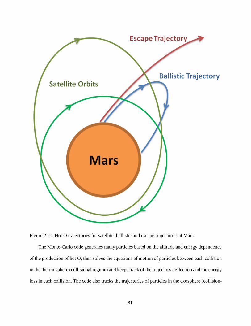
81

Figure 2.21. Hot O trajectories for satellite, ballistic and escape trajectories at Mars.

The Monte-Carlo code generates many particles based on the altitude and energy dependence

of the production of hot O, then solves the equations of motion of particles between each collision

in the thermosphere (collisional regime) and keeps track of the trajectory deflection and the energy

loss in each collision. The code also tracks the trajectories of particles in the exosphere (collision-

82

less regime) as they escape or come back down towards the exobase. The following steps

summarize the algorithm used in the code:

1- Generate a particle (hot O atom) at altitude ‘Z’ with energy ‘E’ with a random velocity direction

(isotropic).

2- Calculate the mean free path: mfp = 1/(nσ)tot.

3- If mfp < 10 km: move in ds = 0.1 mfp steps.

4- If mfp > 10 km: move in ds = 1 km steps.

5- Calculate the trajectory, move the particle for distance ds, and find the new position and the

velocity vector before collision.

6- Calculate the collision probability: ds × (nσ)tot and the probability of collision with species ‘s’:

nsσs/(nσ)tot.

7- Calculate the scattering angle based on energy dependent, forward-peaked differential cross

sections for collision with each species.

8- Calculate the post-collision new velocity vector of the particle according to the conservation of

linear momentum and energy relations.

9- If target is oxygen: Calculate the post-collision direction and energy of the target and go to step

2 for the secondary oxygen.

10- If (E > Emin = 0.01 eV) or (Z < Zmax = 110,000 km) go to step 2, otherwise go to step 1 and

continue for ~107 iterations.

The distinction made in steps 3 and 4 is to ensure that between two collisions, a particle does

not move in a distance greater than 1 km in a single step, since substantial change can happen in

the background neutral densities over one scale height, and thus, the collision probability can

significantly change. All of the particles are created at the Martian sub-solar point, proportional to

the production rate of hot O from 150 km to 500 km in altitude and 0.01 eV to 7.00 eV in energy.

The initial energy determines the initial speed of atoms, and the direction of the velocity vector is

assumed to be isotropic.

83

After each collision, the new velocity vectors for the projectile and the target are calculated

based on random scattering angles drawn from Kharchenko et al. [2000] distributions, and by

utilizing the conservation of linear momentum and energy relations to calculate the energy transfer

between the particles. If the target species is an oxygen atom, it is treated as a secondary and

included in the rest of the simulation. The simulation continues until the particles reach an altitude

of 110,000 km, or their energy drops below 0.01 eV. A spherical bin is placed around Mars at 300

km to record the positions and velocities of the particles as they cross the bin in order to calculate

the hot O distribution function at 300 km.

Figure 2.22 shows the distribution function at 300 km from the two-stream and the Monte-

Carlo calculations. A good agreement is seen between the two simulations at energies below the

escape energy (2 eV), but the Monte-Carlo simulation gives slightly higher densities for escaping

energies. The jump in the density near the escape energy is due to the reflected flux of hot O atoms

for bound trajectories. This effect was incorporated in the two-stream code by adding a down flux

equal to the up flux at the upper-boundary of the code (300 km), for energies below the escape

energy. However, the jump is created naturally in the Monte-Carlo simulation.

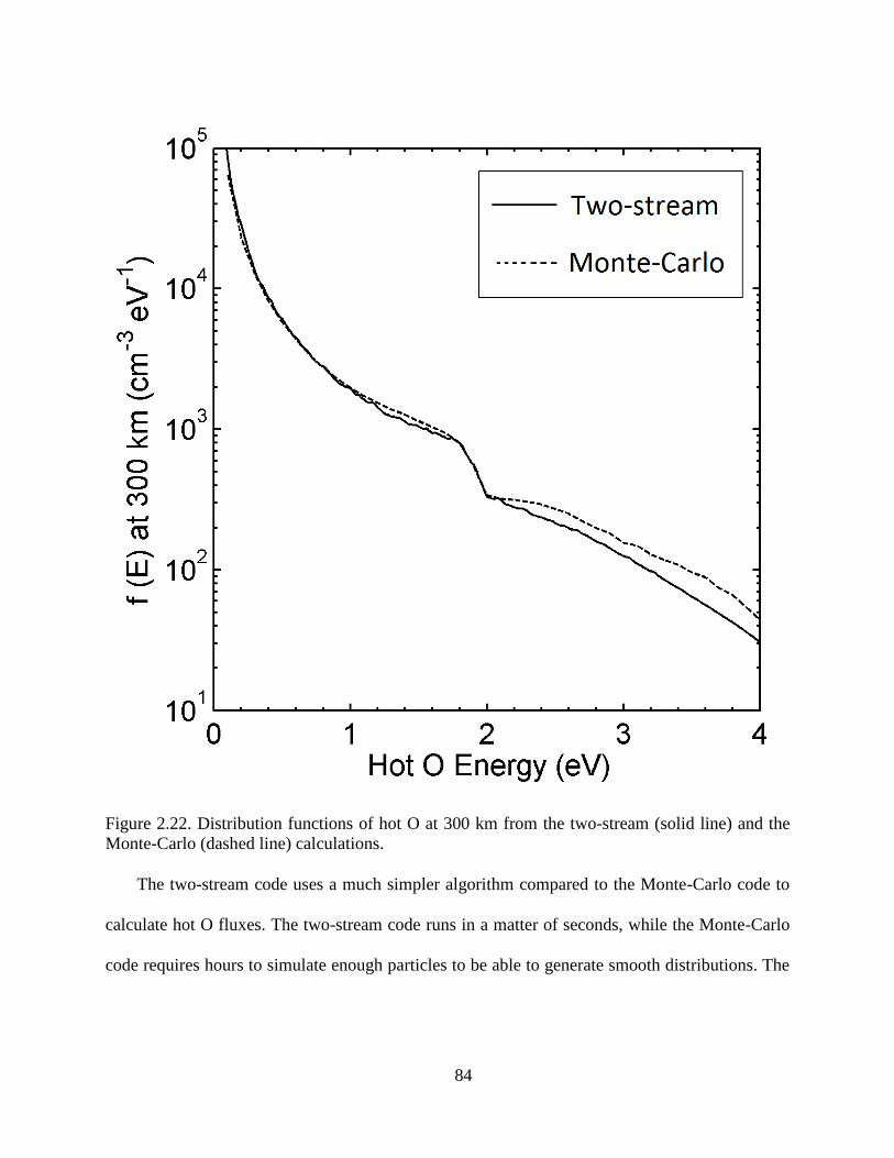
84

Figure 2.22. Distribution functions of hot O at 300 km from the two-stream (solid line) and the

Monte-Carlo (dashed line) calculations.

The two-stream code uses a much simpler algorithm compared to the Monte-Carlo code to

calculate hot O fluxes. The two-stream code runs in a matter of seconds, while the Monte-Carlo

code requires hours to simulate enough particles to be able to generate smooth distributions. The

85

agreement between the two codes gives us confidence in using the two-stream code as a simple

and fast method to calculate hot O fluxes and escape rates at Mars.

2.3 Hot O Escape

Each hot O transport model that calculates hot O fluxes has an escape flux and an escape rate

associated with it. As mentioned in section 2.2.1, hot oxygen escape fluxes of 9 × 107 cm-2 s-1 for

solar maximum and 4 × 107 cm-2 s-1 for solar minimum conditions were predicted by the two

stream code used in this work. By assuming that hot O atoms are escaping only on the dayside of

Mars with uniform distribution, which is only an approximation, one can calculate the escape rate

by multiplying the escape flux by the area of a hemisphere at 300 km:

Escape rate = escape flux × 2π (RM + 300 km)2 = escape flux × (8 × 1017 cm2). 2.20

Therefore, the escape rates on Mars for solar max and min conditions are 7 × 1025 s-1 and 3 ×

1025 s-1, respectively. One can then ask how much oxygen in total these escape rates could have

removed from Mars throughout the Mars history. In order to calculate the amount of oxygen

removed from Mars via the hot O escape process, an overly simplifying assumption has to be

made, i.e., the escape rate has stayed constant over 4.5 billion years of Mars history. This

assumption is not true, since the drivers of escape have significantly changed over time, and also

the Martian atmosphere itself has evolved. Nevertheless, by assuming an average hot O escape

rate of 5 × 1025 s-1 (average between solar max and min escape rates, also valid for solar moderate

conditions) and integrating over 4.5 billion years (1.4 × 1017 s), it turns out that 7 × 1042 oxygen

atoms have escaped from Mars photo-chemically.

86

One can then find the amount of water removed from Mars by the number of escaped oxygen

atoms calculated above, assuming that all of the escaped oxygen atoms initially came from water

[Carr, 1987; Valeille et al., 2010b]. Each water molecule (H2O) contains one oxygen atom, and

by multiplying the number of escaped oxygen atoms by the mass of one water molecule (18 g/mol),

the total mass of removed water is found to be 2 × 1020 g. Dividing this mass by the water density

of 1 g/cm3 gives a total removed volume of 2 × 1020 cm3 or 2 × 105 km3. Assuming that this volume

of water was evenly distributed on the surface of Mars means that a 1-meter layer of water has

been removed from Mars by hot O escape over 4.5 billion years.

2.4 Escape Probability

The two-stream transport code can be used to calculate the probability that a hot oxygen atom

that is created at a certain altitude with a certain energy escapes from Mars. The escape probability

for an oxygen atom created at altitude z with energy E, is defined as the escape flux, divided by

the production rate at altitude z and energy E, divided by the altitude and energy increments used

in the code:

Escape probability = EzEzP

escape

),(

. 2.21

Figure 2.23 shows the two-stream calculation of the dependence of the escape probability on

the production altitude and the nascent energy of hot O atoms for solar maximum conditions. It is

seen that below the escape energy (2 eV), the escape probability is zero, which means none of the

hot O atoms created with energies below the escape energy can escape. Above 2 eV, on the other

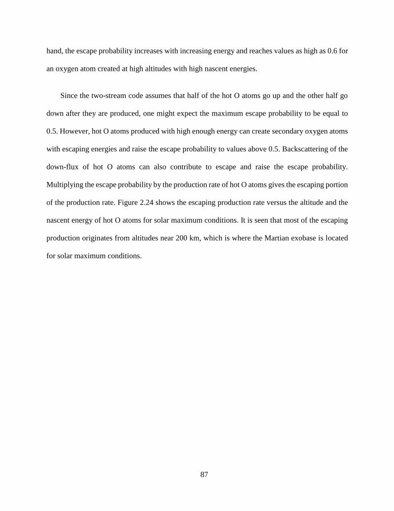
87

hand, the escape probability increases with increasing energy and reaches values as high as 0.6 for

an oxygen atom created at high altitudes with high nascent energies.

Since the two-stream code assumes that half of the hot O atoms go up and the other half go

down after they are produced, one might expect the maximum escape probability to be equal to

0.5. However, hot O atoms produced with high enough energy can create secondary oxygen atoms

with escaping energies and raise the escape probability to values above 0.5. Backscattering of the

down-flux of hot O atoms can also contribute to escape and raise the escape probability.

Multiplying the escape probability by the production rate of hot O atoms gives the escaping portion

of the production rate. Figure 2.24 shows the escaping production rate versus the altitude and the

nascent energy of hot O atoms for solar maximum conditions. It is seen that most of the escaping

production originates from altitudes near 200 km, which is where the Martian exobase is located

for solar maximum conditions.

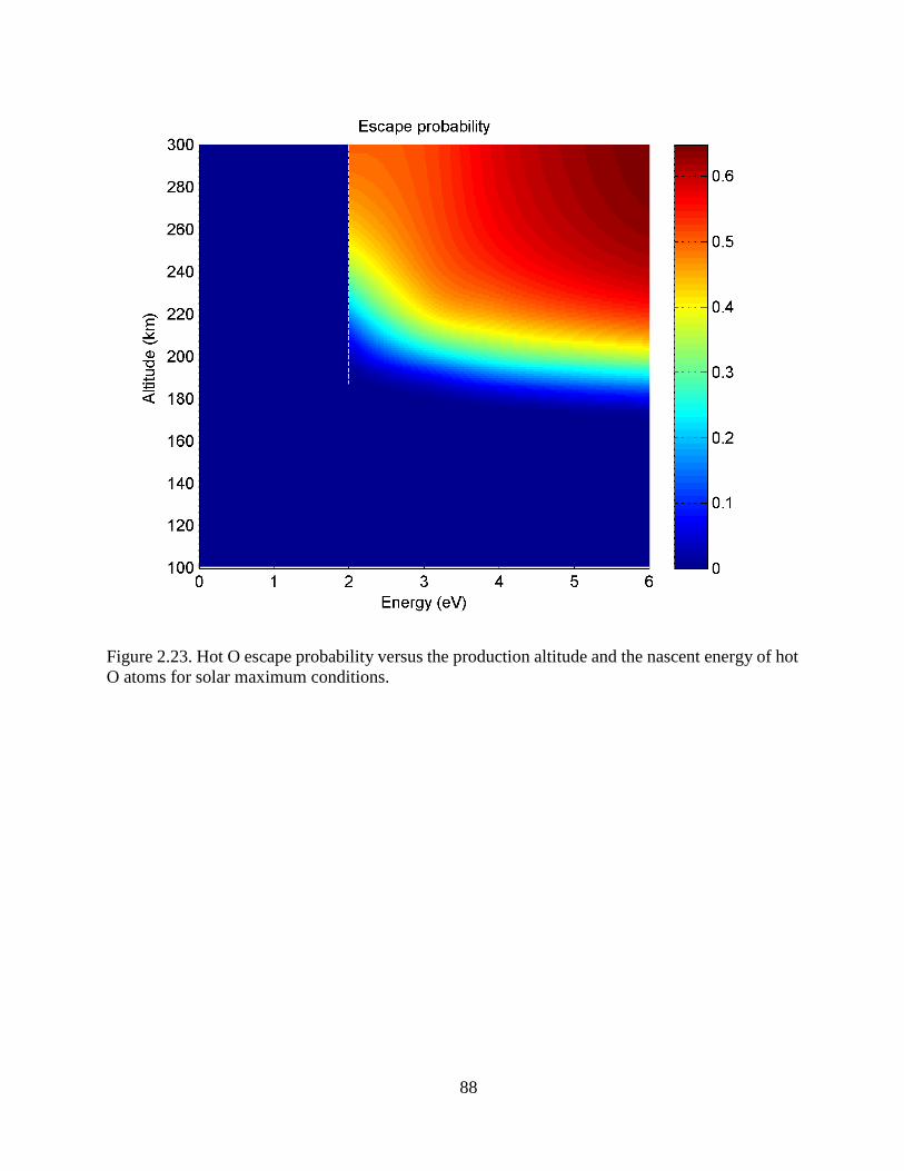
88

Figure 2.23. Hot O escape probability versus the production altitude and the nascent energy of hot

O atoms for solar maximum conditions.

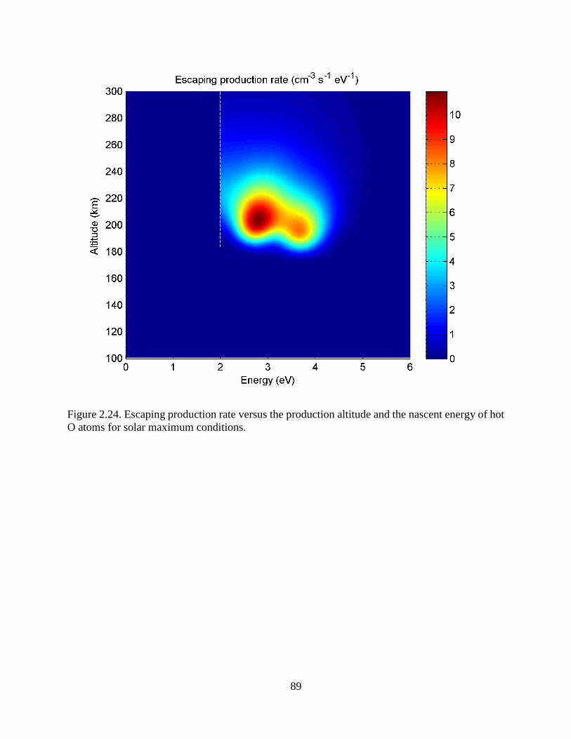
89

Figure 2.24. Escaping production rate versus the production altitude and the nascent energy of hot

O atoms for solar maximum conditions.

90

3 Oxygen and Hydrogen Pickup Ions at Mars

Mars has an extended exosphere consisting of oxygen and hydrogen atoms. Ionization of these

atoms creates ions that are picked up by the solar wind electric and magnetic fields, energized, and

therefore detectable by spacecraft instruments. In this chapter the sources of production of these

pickup ions are described, the equations of motion of pickup ions are derived and solved, and a

pickup trajectory solver model is used to calculate the flux of oxygen and hydrogen pickup ions

outside the Martian bow shock for different solar wind conditions.

The oxygen exosphere at Mars is mainly populated by hot oxygen atoms that are created in

the ionosphere via the dissociative recombination of O2+ molecules with electrons. The hot oxygen

exospheric profile used as the source for oxygen pickup ions in this work was described in Chapter

2. The hydrogen exosphere is populated by thermal hydrogen atoms from the tail of the Maxwell-

Boltzmann distribution, which contribute to Jeans escape. Non-thermal processes also create a

bound corona that consists of carbon and nitrogen atoms, as well as CO2 molecules. These bound

species mainly stay inside the Martian bow shock, cannot escape, and do not create a detectable

pickup ion flux outside the bow shock.

The ultraviolet spectrometers onboard the Mariner 6 and 7 spacecraft first detected the Lyman

α emission from the extended hydrogen exosphere of Mars in 1969 [Anderson and Hord, 1971]

followed by similar measurements by the Mariner 9 [Anderson, 1974], and also the Mars 2 and 3

spacecraft. The Phobos-2 spacecraft also detected hydrogen pickup ions associated with the neutral

hydrogen exosphere of Mars [Barabash et al., 1991] and the more recent pickup proton

measurements by the ASPERA 3 Ion Mass Analyzer on the Mars Express spacecraft reaffirmed

91

the observations of Phobos-2 [Dubinin et al., 2006]. The Lyman α emission from the hydrogen

exosphere of Mars was also detected by the neutral particle detector of the ASPERA-3 instrument

[Galli et al., 2006] as well as the ultraviolet spectrometers SPICAM on Mars Express [Chaufray

et al., 2008], Alice on Rosetta [Feldman et al., 2011], and IUVS on MAVEN [Chaffin et al., 2015].

Recent studies indicate a significant seasonal variation of the Mars hydrogen exosphere. This

variation has been observed by Lyman α measurements of the scattered solar radiation using the

Hubble Space Telescope [Clarke et al., 2014; Bhattacharyya et al., 2015], as well as the ASPERA

3 measurements of pickup hydrogen ions [Yamauchi et al., 2015]. Chaufray et al. [2015a] modeled

the diurnal, seasonal, and solar activity dependent variation of the hydrogen exosphere and also

found that the Martian hydrogen corona and the associated Jeans escape can have significant

temporal variations. The exospheric hydrogen density profile used as the source of pickup

hydrogen ions for the calculations done in this chapter is adapted from Feldman et al. [2011].

Figure 3.1 shows the exospheric profiles used for neutral oxygen and hydrogen sources of pickup

ions.

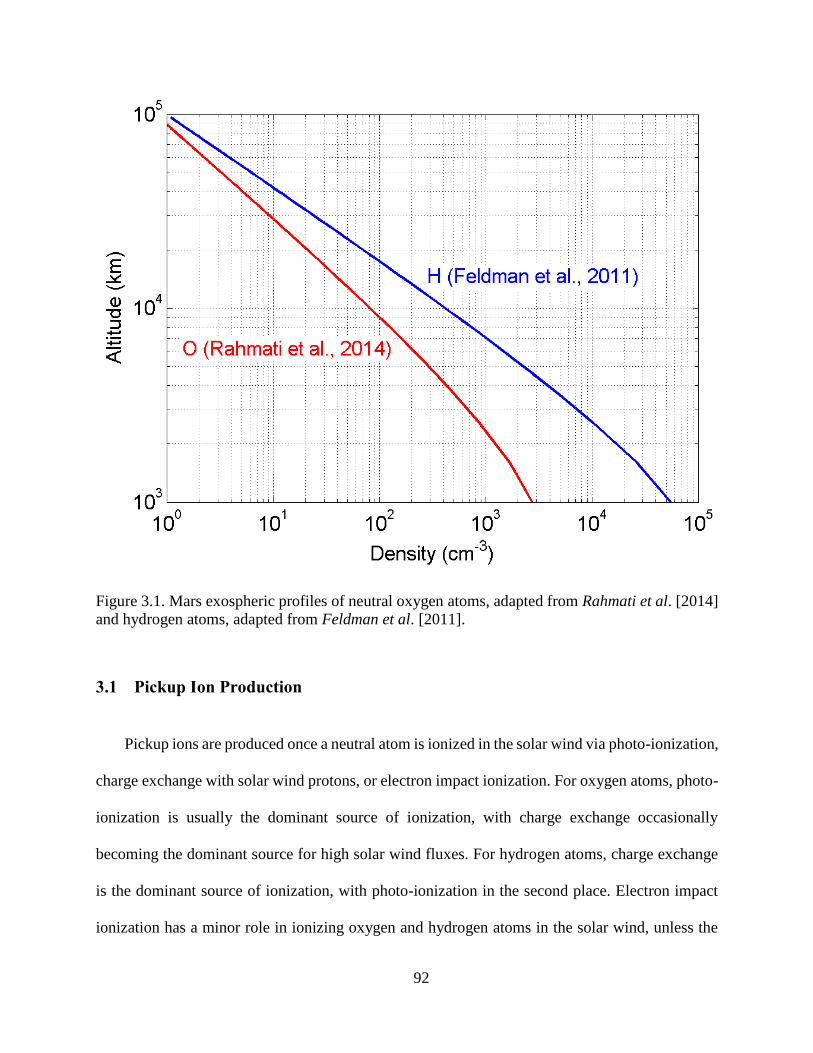
92

Figure 3.1. Mars exospheric profiles of neutral oxygen atoms, adapted from Rahmati et al. [2014]

and hydrogen atoms, adapted from Feldman et al. [2011].

3.1 Pickup Ion Production

Pickup ions are produced once a neutral atom is ionized in the solar wind via photo-ionization,

charge exchange with solar wind protons, or electron impact ionization. For oxygen atoms, photo-

ionization is usually the dominant source of ionization, with charge exchange occasionally

becoming the dominant source for high solar wind fluxes. For hydrogen atoms, charge exchange

is the dominant source of ionization, with photo-ionization in the second place. Electron impact

ionization has a minor role in ionizing oxygen and hydrogen atoms in the solar wind, unless the

93

solar wind electron temperature and density becomes unusually high. This section describes each

of the ionization processes in detail, providing cross sections for each process and calculating the

respective ionization frequencies.

3.1.1 Photo-ionization

Solar photons with energies above the ionization potential of neutral species within the

Martian exosphere can ionize the neutrals. For oxygen and hydrogen atoms the ionization potential

is ~13.6 eV, requiring a photon wavelength of ~90 nm or less for ionization. Therefore, solar

radiation below 90 nm can cause photo-ionization of exospheric oxygen and hydrogen atoms,

represented by:

hv + H → H+ + e-, 3.1

hv + O → O+ + e-, 3.2

where h is the Planck’s constant, and v is the frequency of the solar photon, calculated according

to:

v = c / λ, 3.3

where c is the speed of light, and λ is the photon wavelength. In the above equations, hv represents

the energy of a photon calculated according to:

E = hv = h c / λ. 3.4

The ejected electron carries away the energy of the incident photon minus the ionization

potential of the neutral species. The photo-ionization frequency for each species is calculated

according to:

94

IPI = ∫ σPI (λ) ϕEUV (λ) dλ, 3.5

where σPI (λ) is the wavelength dependent cross section for photo-ionization of the neutral species,

ϕEUV (λ) is the wavelength dependent solar photon flux, and λ is the photon wavelength.

Figure 3.2 shows the cross sections used for photo-ionization of atomic oxygen and hydrogen.

The photo-ionization cross section for atomic oxygen is adapted from Angel and Samson [1988],

and for atomic hydrogen from http://phidrates.space.swri.edu. The bumps in the oxygen cross

section curve are due to different transitions within the electronic levels of atomic oxygen, whereas

for atomic hydrogen the only ionization route is through taking out the single electron from the 1S

energy level, hence the smooth cross section curve. Both oxygen and hydrogen atoms are assumed

to be initially electronically relaxed, i.e., not in excited states.

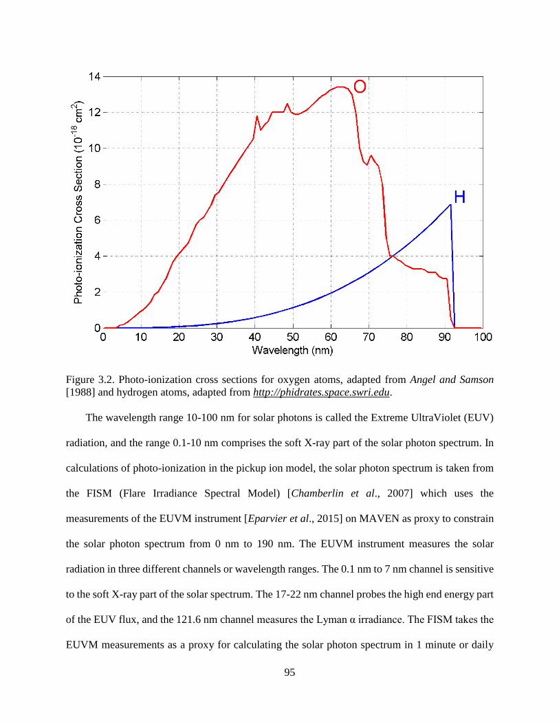
95

Figure 3.2. Photo-ionization cross sections for oxygen atoms, adapted from Angel and Samson

[1988] and hydrogen atoms, adapted from http://phidrates.space.swri.edu.

The wavelength range 10-100 nm for solar photons is called the Extreme UltraViolet (EUV)

radiation, and the range 0.1-10 nm comprises the soft X-ray part of the solar photon spectrum. In

calculations of photo-ionization in the pickup ion model, the solar photon spectrum is taken from

the FISM (Flare Irradiance Spectral Model) [Chamberlin et al., 2007] which uses the

measurements of the EUVM instrument [Eparvier et al., 2015] on MAVEN as proxy to constrain

the solar photon spectrum from 0 nm to 190 nm. The EUVM instrument measures the solar

radiation in three different channels or wavelength ranges. The 0.1 nm to 7 nm channel is sensitive

to the soft X-ray part of the solar spectrum. The 17-22 nm channel probes the high end energy part

of the EUV flux, and the 121.6 nm channel measures the Lyman α irradiance. The FISM takes the

EUVM measurements as a proxy for calculating the solar photon spectrum in 1 minute or daily

http://phidrates.space.swri.edu/

96

averaged cadences with a 1 nm resolution. Figure 3.3 shows a daily averaged solar photon

irradiance constructed by FISM for 3 February 2015 as constrained by the EUVM measurements

at Mars. Figure 3.4 shows the same solar spectrum, this time in units of flux, ϕEUV (λ), which can

be used to calculate photo-ionization frequencies using Equation 3.5. The calculated photo-

ionization frequency for this solar flux is 2.2 × 10-7 s-1 for oxygen and 8.4 × 10-8 s-1 for hydrogen

atoms.

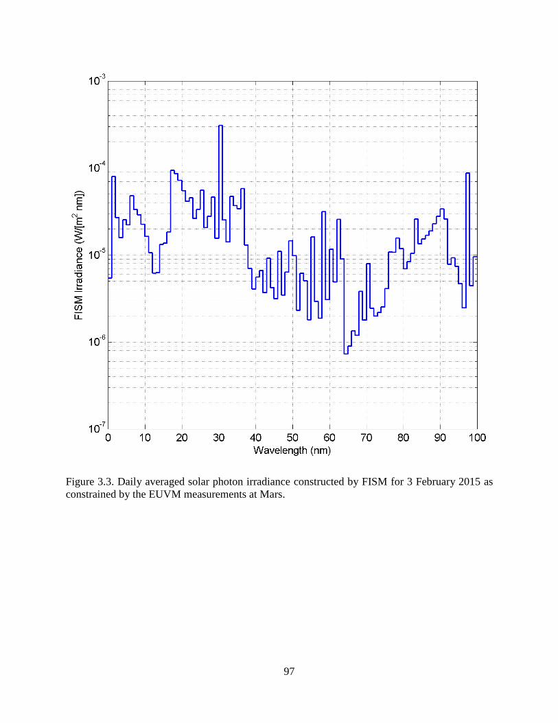
97

Figure 3.3. Daily averaged solar photon irradiance constructed by FISM for 3 February 2015 as

constrained by the EUVM measurements at Mars.

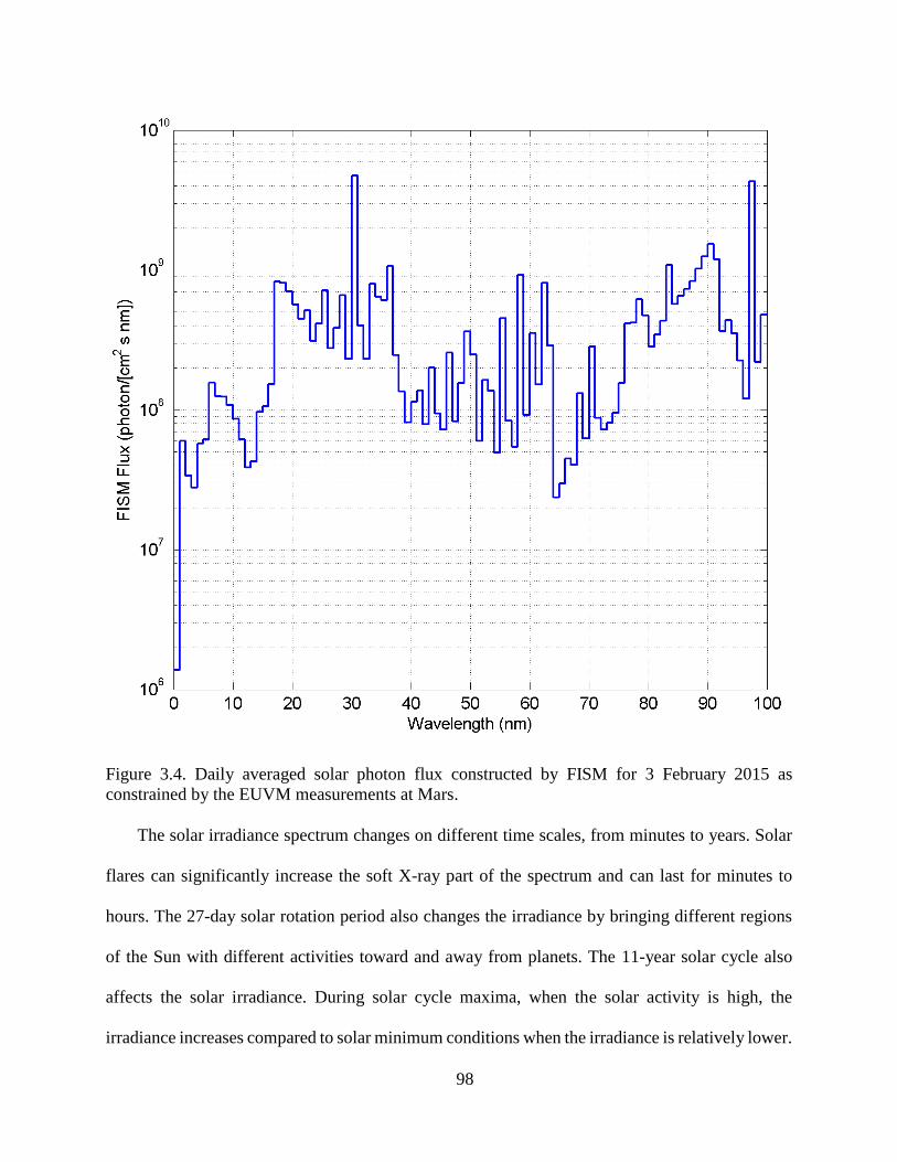
98

Figure 3.4. Daily averaged solar photon flux constructed by FISM for 3 February 2015 as

constrained by the EUVM measurements at Mars.

The solar irradiance spectrum changes on different time scales, from minutes to years. Solar

flares can significantly increase the soft X-ray part of the spectrum and can last for minutes to

hours. The 27-day solar rotation period also changes the irradiance by bringing different regions

of the Sun with different activities toward and away from planets. The 11-year solar cycle also

affects the solar irradiance. During solar cycle maxima, when the solar activity is high, the

irradiance increases compared to solar minimum conditions when the irradiance is relatively lower.

99

The distance between Mars and the Sun also plays an important role in the amount of solar

radiation that reaches Mars. The solar photon flux scales according to the inverse square law:

ϕEUV ~ 1/r2, 3.6

where r is the distance between the Sun and an object in the solar system. Since Mars has an elliptic

orbit around the Sun, it receives a more intense radiation at its perihelion when it is closest to the

Sun compared to its aphelion when it is farthest away from the Sun. At its perihelion, Mars is at

1.38 AU, and at its aphelion at 1.67 AU from the Sun. Thus, the high orbital eccentricity of Mars

alone accounts for a 45% increase in the solar radiation reaching Mars at perihelion compared to

aphelion.

The photo-ionization of hydrogen and oxygen atoms outside the Martian bow shock is

optically thin, meaning that the ionizing solar EUV flux is not attenuated due to absorption by

exospheric neutrals, since the neutral densities are very low at distances outside the bow shock.

Therefore, in calculating photo-ionization frequencies the attenuation in the solar flux is ignored

and we assume a constant solar flux vs. altitude outside the bow shock.

3.1.2 Charge Exchange

Collisions of solar wind protons with the exospheric species can result in the charge exchange

process in which an electron is transferred from the neutral atom to the solar wind proton, creating

an ion and a fast hydrogen atom:

psw + H → H(fast) + H+, 3.7

psw + O → H(fast) + O+, 3.8

where psw is a solar wind proton.

100

The charge exchange frequency is calculated according to:

ICX = σCX ϕsw = σCX nsw Usw, 3.9

where σCX is the cross section for charge exchange between a solar wind proton and the neutral

species, and ϕsw is the solar wind proton flux, nsw is the solar wind density, and Usw is the solar

wind speed.

The assumed cross section for the proton-atomic hydrogen charge exchange is 2 × 10-15 cm2

adapted from Fite et al. [1960] and for the proton-atomic oxygen charge exchange is 8 × 10-16 cm2

adapted from Stebbings et al. [1964]. These cross sections are in fact energy dependent and the

values provided are only accurate within a factor of two for solar wind protons with energies

between 500 eV to 2 keV, corresponding to solar wind speeds of ~300 km/s to ~600 km/s.

The solar wind flux is highly variable in timescales of hours to days. Solar wind speeds can

be as low as 300 km/s for quiet times, and as high as 1000 km/s for disturbed solar wind conditions

such as the passage of an Interplanetary Coronal Mass Ejection (ICME). Statistically, the solar

wind speed does not have a dependence on the distance from the Sun for radial distances farther

than the orbit of Mercury. The solar wind density and therefore flux, on the other hand, both scale

as:

nsw ~ ϕsw ~ 1/r2, 3.10

and decrease with increasing the distance from the Sun according to the inverse square law. The

solar wind density at Mars ranges from ~1 cm-3 to up to 20 cm-3, and as a result, the solar wind

flux and the corresponding charge exchange frequencies can have variations as high as a factor of

~50. Nevertheless, the typical solar wind at Mars has a speed of around 400 km/s, with a density

101

of ~2.5 cm-3, giving a solar wind flux of 108 cm-2 s-1. The charge exchange ionization frequency

for this flux is 8 × 10-8 s-1 for oxygen and 2 × 10-7 s-1 for hydrogen atoms.

In calculating the charge exchange frequencies in the pickup ion model, the solar wind flux is

taken from solar wind ion measurements by the SWIA (Solar Wind Ion Analyzer) instrument

[Halekas et al., 2013] on MAVEN. SWIA is an electrostatic analyzer that can measure the energy

to charge ratio of ions by creating a potential difference between two hemispheres. SWIA has 24

anodes that resolve the angular distribution of ions in azimuth and uses electrostatic deflection to

sweep ±45° in elevation for energy to charge ratios below 5 keV/e, giving it a 2.8 π sr solid angle

coverage of the sky.

The charge exchange process removes part of the solar wind protons by neutralizing them and

turning them into fast hydrogen atoms. These Energetic Neutral Atoms (ENA’s) no longer feel the

electric and magnetic fields in the solar wind and do not respond to the bow shock at Mars, and

thus pass through the bow shock without getting deflected. The ENA’s can, therefore, penetrate

deep into the upper atmosphere and deposit their energy by collisions with atmospheric neutrals.

These ENA’s can also experience a second charge exchange reaction and lose an electron to the

background species and become ionized again. The SWIA instrument detected protons near the

periapses of MAVEN’s dayside orbits that were created via this “double charge exchange” process

[Halekas et al., 2015].

3.1.3 Electron Impact

Solar wind electrons can ionize the neutral atoms in the Martian exosphere via the electron

impact ionization process:

102

e- + H → H+ + 2e-, 311.

e- + O → O+ + 2e-. 3.12

In this process an electron with an energy greater than the ionization potential of the neutral

species impacts the neutral and removes an electron from the neutral atom, thereby ionizing it. The

electron impact ionization frequency is calculated according to:

IEI = ∫ σEI (E) ϕe (E) dE, 3.13

where σEI (E) is the energy dependent cross section for electron impact with neutral species leading

to ionization, ϕe(E) is the energy dependent angle integrated (omni-directional) solar wind electron

flux, and E is the energy of electrons.

Figure 3.5 shows the cross sections used for the electron impact processes adapted from

Cravens et al. [1987]. The electron impact ionization cross section for hydrogen peaks at ~50 eV,

and for oxygen at ~70 eV. Electron impact plays a minor role in ionizing oxygen and hydrogen

atoms in the solar wind, when the solar wind has its typical electron temperature of ~10 eV, and

therefore the bulk of the electron spectrum lies below the ionization threshold of exospheric

neutrals (~14 eV). On the contrary, electron impact can dominate photo-ionization and charge

exchange within the magneto-sheath of Mars, where electrons are heated to energies around and

even above ~100 eV with elevated densities.

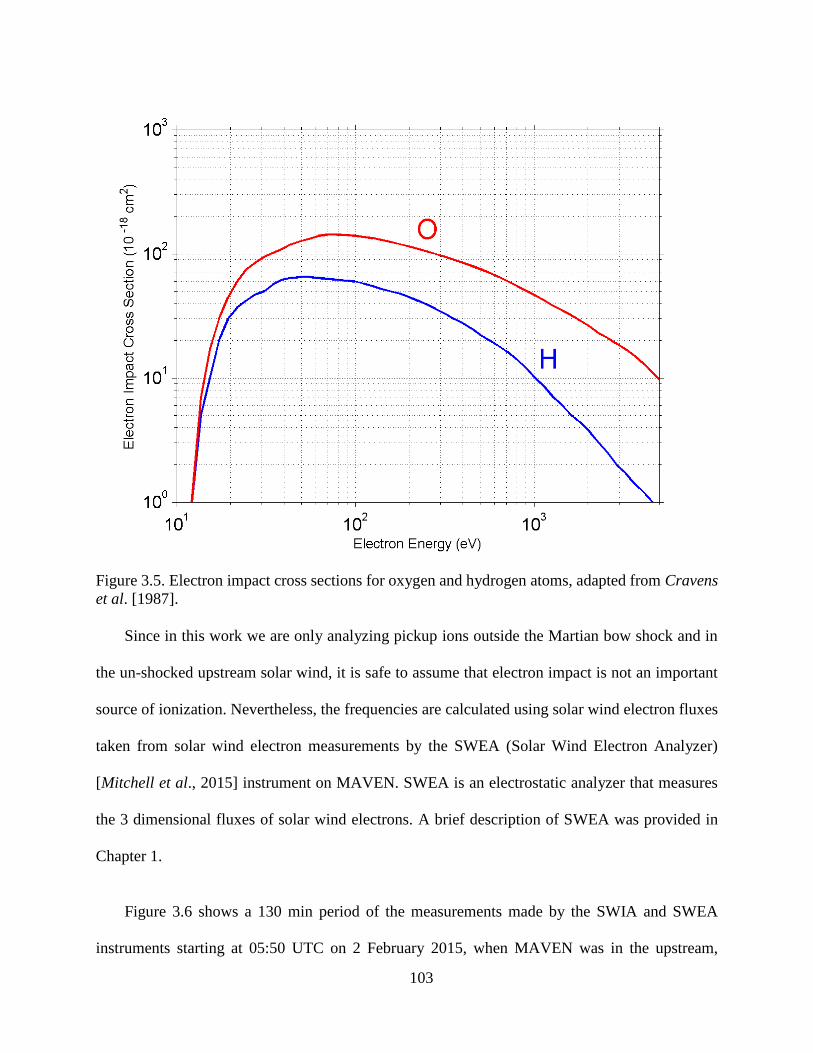
103

Figure 3.5. Electron impact cross sections for oxygen and hydrogen atoms, adapted from Cravens

et al. [1987].

Since in this work we are only analyzing pickup ions outside the Martian bow shock and in

the un-shocked upstream solar wind, it is safe to assume that electron impact is not an important

source of ionization. Nevertheless, the frequencies are calculated using solar wind electron fluxes

taken from solar wind electron measurements by the SWEA (Solar Wind Electron Analyzer)

[Mitchell et al., 2015] instrument on MAVEN. SWEA is an electrostatic analyzer that measures

the 3 dimensional fluxes of solar wind electrons. A brief description of SWEA was provided in

Chapter 1.

Figure 3.6 shows a 130 min period of the measurements made by the SWIA and SWEA

instruments starting at 05:50 UTC on 2 February 2015, when MAVEN was in the upstream,

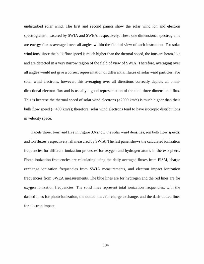
104

undisturbed solar wind. The first and second panels show the solar wind ion and electron

spectrograms measured by SWIA and SWEA, respectively. These one dimensional spectrograms

are energy fluxes averaged over all angles within the field of view of each instrument. For solar

wind ions, since the bulk flow speed is much higher than the thermal speed, the ions are beam-like

and are detected in a very narrow region of the field of view of SWIA. Therefore, averaging over

all angles would not give a correct representation of differential fluxes of solar wind particles. For

solar wind electrons, however, this averaging over all directions correctly depicts an omni-

directional electron flux and is usually a good representation of the total three dimensional flux.

This is because the thermal speed of solar wind electrons (>2000 km/s) is much higher than their

bulk flow speed (~ 400 km/s); therefore, solar wind electrons tend to have isotropic distributions

in velocity space.

Panels three, four, and five in Figure 3.6 show the solar wind densities, ion bulk flow speeds,

and ion fluxes, respectively, all measured by SWIA. The last panel shows the calculated ionization

frequencies for different ionization processes for oxygen and hydrogen atoms in the exosphere.

Photo-ionization frequencies are calculating using the daily averaged fluxes from FISM, charge

exchange ionization frequencies from SWIA measurements, and electron impact ionization

frequencies from SWEA measurements. The blue lines are for hydrogen and the red lines are for

oxygen ionization frequencies. The solid lines represent total ionization frequencies, with the

dashed lines for photo-ionization, the dotted lines for charge exchange, and the dash-dotted lines

for electron impact.

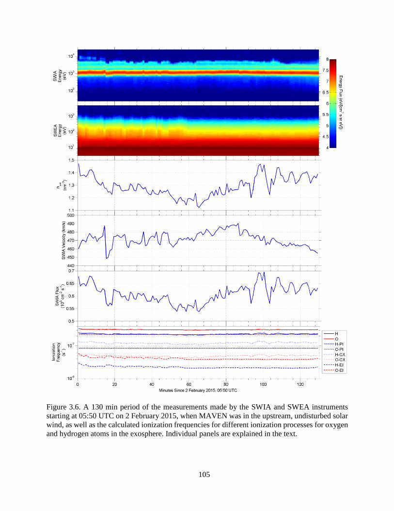
105

Figure 3.6. A 130 min period of the measurements made by the SWIA and SWEA instruments

starting at 05:50 UTC on 2 February 2015, when MAVEN was in the upstream, undisturbed solar

wind, as well as the calculated ionization frequencies for different ionization processes for oxygen

and hydrogen atoms in the exosphere. Individual panels are explained in the text.

106

A snapshot of the spectra in the first and the second panels of Figure 3.6 at the 60-minute

mark is shown in Figure 3.7. The curves are energy fluxes of electrons and ions measured by SWIA

and SWEA, respectively. For the electron spectrum, the ledge at ~10 eV is the spacecraft photo-

electrons that create a cloud around the spacecraft due to the few volts positive spacecraft potential

in the sunlit part of the orbit. These spacecraft photo-electrons have energies that are below the

ionization threshold for oxygen and hydrogen atoms; therefore, they have minimal impact on

electron impact ionization calculations and there is no need to correct the spectrum in order to

remove these photo-electrons. However, the positive spacecraft potential that is created due to the

ejection of photo-electrons can artificially boost the low energy part of the spectrum by attracting

the solar wind electrons toward the detector.

For ions the peak at 1.2 keV is due to the solar wind protons, and the secondary peak at 2.4

keV/e is due to the doubly ionized solar wind alpha particles (He++). Since SWIA measures the

energy to charge ratio of ions, solar wind alpha particles have energies that are twice that shown

in Figure 3.7. The third peak at around 4 keV is due to pickup hydrogen fluxes, which are very

variable and will be described in the next two sections. Figure 3.8 shows the same electron and ion

spectrum, this time in units of flux, instead of energy flux.

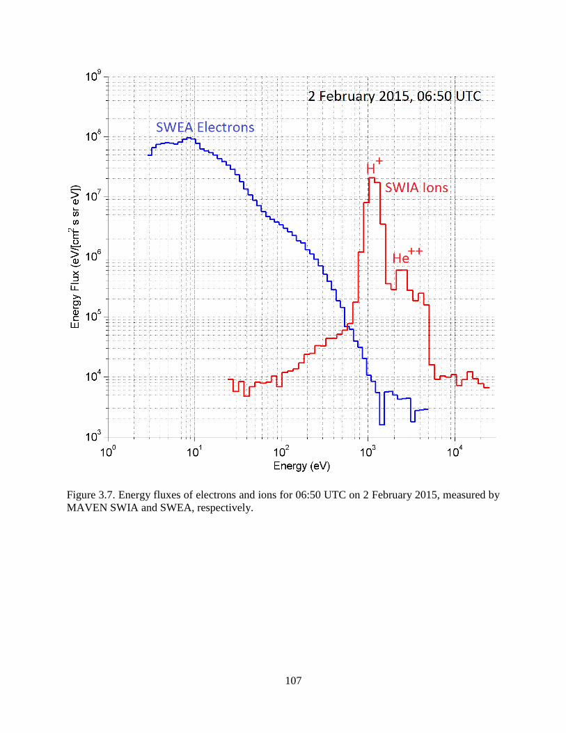
107

Figure 3.7. Energy fluxes of electrons and ions for 06:50 UTC on 2 February 2015, measured by

MAVEN SWIA and SWEA, respectively.

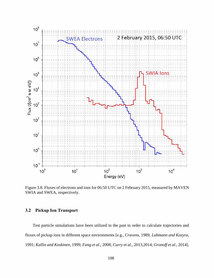
108

Figure 3.8. Fluxes of electrons and ions for 06:50 UTC on 2 February 2015, measured by MAVEN

SWIA and SWEA, respectively.

3.2 Pickup Ion Transport

Test particle simulations have been utilized in the past in order to calculate trajectories and

fluxes of pickup ions in different space environments [e.g., Cravens, 1989; Luhmann and Kozyra,

1991; Kallio and Koskinen, 1999; Fang et al., 2008; Curry et al., 2013,2014; Gronoff et al., 2014].

109

Test particle simulations of oxygen pickup ions at Mars create many oxygen ions with probabilities

proportional to the ionization rate of neutral oxygen at random locations around Mars. The number

of particles simulated in different studies ranges from thousands to billions, depending on

resolution requirements and computational resources. After creating each particle, the codes then

numerically solve the equations of motion of the particles, calculating their trajectory in the

background electric and magnetic fields. The fields are usually adapted from MHD (Magneto-

Hydro-Dynamic) or hybrid (ions treated as particles, electrons treated as a neutralizing fluid)

simulations and assumed to be static, i.e., not updated in each time step of the simulation. Certain

planar bins are placed in specific locations to record the velocity components of particles crossing

the bins. The number of particles crossing each bin along with their associated velocities is used

to calculate the flux of particles in each bin.

As part of this project, a pickup ion trajectory solver code was developed that keeps track of

the trajectories of pickup ions in the solar wind. The equations of motion of ions are analytically

solved with the assumption that the fields are uniform for simulation regions outside the bow shock

and in the undisturbed upstream solar wind. Once a pickup ion is created in the solar wind, it senses

the solar wind magnetic field, B, is “picked up” and starts to gyrate around the magnetic field line,

and at the same time drifts along with the solar wind.

The gyro-frequency of a pickup ion is calculated according to:

Ω = q B / m, 3.14

where q is the electric charge of the pickup ion, B is the magnetic field strength, and m is the mass

of the pickup ion. For a typical solar wind magnetic field of B = 5 nT, the hydrogen and oxygen

gyro-frequencies are ΩH = 0.48 rad/s and ΩO = 0.03 rad/s, respectively.

110

One gyro-period is the time it takes a pickup ion to complete one full gyro-motion about the

magnetic field line. The gyro-period of a pickup ion is calculated according to:

T = 2π / Ω, 3.15

and using the same parameters as above, it is equal to TH = 13 s and TO = 209 s, for hydrogen and

oxygen pickup ions, respectively.

The gyro-radius of a pickup ion is calculated according to:

R = Usw┴ / Ω, 3.16

where Usw ┴ is the perpendicular component of the solar wind velocity, Usw, relative to the direction

of the magnetic field, B. For an angle θUB between the solar wind velocity and the direction of the

embedded magnetic field,

Usw ┴ = Usw sin(θUB), 3.17

and R takes the form of:

R = Usw sin(θUB) / Ω = m Usw sin(θUB) / q B. 3.18

Assuming a typical solar wind speed of 400 km/s with θUB = π/2 and using the same

parameters as above, the hydrogen and oxygen pickup ion gyro-radii are equal to RH = 830 km

and RO = 13,000 km, respectively.

The angle between B and Usw is also called the IMF (Interplanetary Magnetic Field) cone

angle and can range from 0° to 180°, with 0° corresponding to a magnetic field pointing in the

same direction as the solar wind bulk flow velocity, 90° corresponding to an IMF normal to Usw,

111

and 180° corresponding to an anti-solar wind directed IMF. In one gyro-period, pickup ions move

downstream by a distance of:

Δx = Usw┴ T = 2π R. 3.19

The maximum speed of a pickup ion in the solar wind with respect to a stationary object is

achieved when it is in the middle of one gyro-period, and can be calculated according to:

Vmax = 2 Usw┴ = 2 Usw sin(θUB). 3.20

Therefore, the maximum energy of a pickup ion is given as:

Emax = ½ m Vmax 2 = ½ m (2 Usw

┴) 2 = 2 m Usw2 sin2(θUB). 3.21

Given the parameters above, hydrogen and oxygen pickup ions have maximum energies of

EH = 3.3 keV, and EO = 53 keV, respectively.

In order to track the transport of pickup ions, the equations of motion of pickup ions need to

be solved:

F = m dv/dt = q (E + v × B), 3.22

where v is the velocity of the pickup ion, and F is the Lorentz force acting on the pickup ion due

to the solar wind magnetic field and its associated motional electric field (or convective electric

field),

E = - Usw × B. 3.23

The motional electric field, E, is perpendicular to both the solar wind velocity and the

magnetic field. Substituting the motional electric field in the equations of motion gives:

m �̇� = q (- Usw × B + v × B) = q (- Usw + v) × B, 3.24

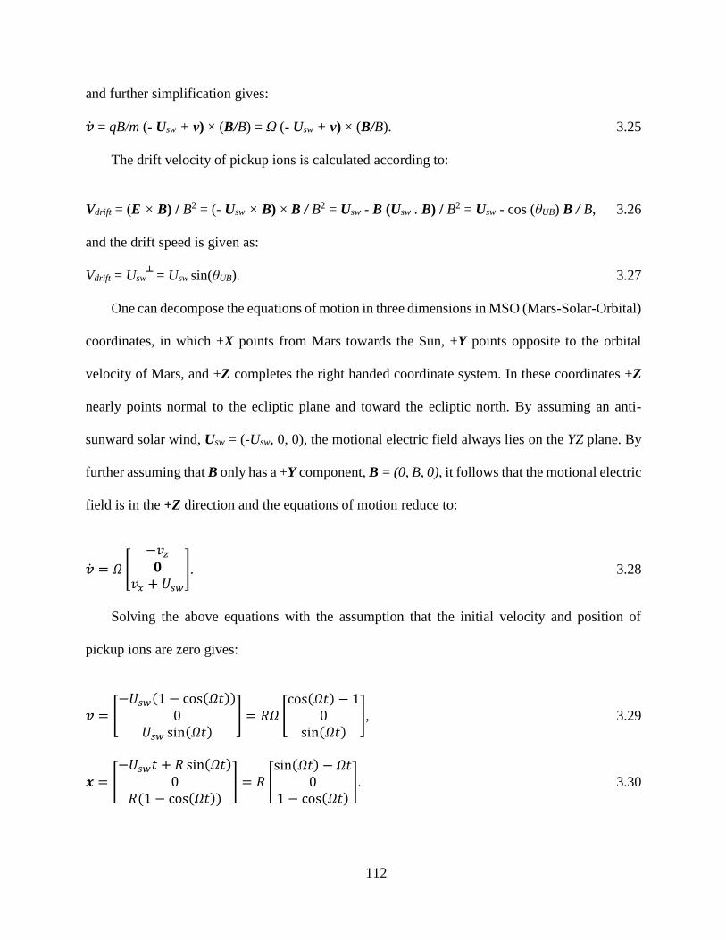
112

and further simplification gives:

�̇� = qB/m (- Usw + v) × (B/B) = Ω (- Usw + v) × (B/B). 3.25

The drift velocity of pickup ions is calculated according to:

Vdrift = (E × B) / B2 = (- Usw × B) × B / B2 = Usw - B (Usw . B) / B2 = Usw - cos (θUB) B / B, 3.26

and the drift speed is given as:

Vdrift = Usw┴ = Usw sin(θUB). 3.27

One can decompose the equations of motion in three dimensions in MSO (Mars-Solar-Orbital)

coordinates, in which +X points from Mars towards the Sun, +Y points opposite to the orbital

velocity of Mars, and +Z completes the right handed coordinate system. In these coordinates +Z

nearly points normal to the ecliptic plane and toward the ecliptic north. By assuming an anti-

sunward solar wind, Usw = (-Usw, 0, 0), the motional electric field always lies on the YZ plane. By

further assuming that B only has a +Y component, B = (0, B, 0), it follows that the motional electric

field is in the +Z direction and the equations of motion reduce to:

�̇� = 𝛺 [

−𝑣𝑧𝟎

𝑣𝑥 + 𝑈𝑠𝑤]. 3.28

Solving the above equations with the assumption that the initial velocity and position of

pickup ions are zero gives:

𝒗 = [−𝑈𝑠𝑤(1 − cos(𝛺𝑡))

0𝑈𝑠𝑤 sin(𝛺𝑡)

] = 𝑅𝛺 [cos(𝛺𝑡) − 1

0sin(𝛺𝑡)

], 3.29

𝒙 = [−𝑈𝑠𝑤𝑡 + 𝑅 sin(𝛺𝑡)

0𝑅(1 − cos(𝛺𝑡))

] = 𝑅 [sin(𝛺𝑡) − 𝛺𝑡

01 − cos(𝛺𝑡)

]. 3.30

113

To further generalize the solutions, one can relax the assumption that B is perpendicular to

Usw and attempt to solve the equations of motion. Here we assume that B is on the XY (~ecliptic)

plane, with a positive Y component, and that B makes an angle θUB with the direction of the solar

wind bulk flow:

𝑩 = B[− cos(𝜃𝑈𝐵)sin(𝜃𝑈𝐵)

0

]. 3.31

In this case the motional electric field will still be in the +Z direction and the equations of

motion take the following form:

�̇� = 𝛺 [

−𝑣𝑧 sin(𝜃𝑈𝐵)−𝑣𝑧 cos(𝜃𝑈𝐵)

(𝑣𝑥 + 𝑈𝑠𝑤) sin(𝜃𝑈𝐵) + 𝑣𝑦 cos(𝜃𝑈𝐵)]. 3.32

Solving the above equations with the assumption that the initial velocity and position of

pickup ions is zero gives:

𝒗 = [

−𝑈𝑠𝑤 sin2(𝜃𝑈𝐵) (1 − cos(𝛺𝑡))

−𝑈𝑠𝑤 sin(𝜃𝑈𝐵) cos(𝜃𝑈𝐵) (1 − cos(𝛺𝑡))

𝑈𝑠𝑤 sin(𝜃𝑈𝐵) sin(𝛺𝑡)

] = 𝑅𝛺 [

sin(𝜃𝑈𝐵) (cos(𝛺𝑡) − 1)

cos(𝜃𝑈𝐵) (cos(𝛺𝑡) − 1)

sin(𝛺𝑡)], 3.33

𝒙 = [

sin(𝜃𝑈𝐵) (− sin(𝜃𝑈𝐵)𝑈𝑠𝑤𝑡 + 𝑅 sin(𝛺𝑡))

cos(𝜃𝑈𝐵) (− sin(𝜃𝑈𝐵)𝑈𝑠𝑤𝑡 + 𝑅 sin(𝛺𝑡))

𝑅(1 − cos(𝛺𝑡))

] = 𝑅 [

sin(𝜃𝑈𝐵) (sin(Ωt) − 𝛺𝑡)

cos(𝜃𝑈𝐵) (sin(Ωt) − 𝛺𝑡)

1 − cos(𝛺𝑡)]. 3.34

In reality B does not always lie on the XY plane, nor does E always point in the +Z direction.

In order to generalize the solutions for any given B direction, the code assumes that the coordinate

system is initially rotated so that B is already on the XY plane (with a +Z electric field), calculates

the pickup ion trajectories and then rotates the coordinate system back to the original orientation.

Therefore, after solving the trajectories, only one rotation is needed about the X axis by the angle

that E makes with +Z, which is called the motional electric field clock angle:

114

ϕEZ = atan2 (-Bz , By). 3.35

This angle can range between 0° and 360°; thereby, necessitating the use of a four quadrant

inverse tangent calculator (atan2). This rotation brings E back to its original orientation and

generalizes the trajectories for any given B.

So far we assumed that Usw is anti-sunward. Actual measurements from the SWIA instrument

onboard MAVEN reveal that Usw can have off-axis components that can be as high as 20% of the

solar wind speed. Therefore, it is necessary to take these “cross-wind” components into account

when finding pickup ion trajectories. To achieve this end, the pickup ion code first rotates the

coordinate system to bring Usw in the anti-sunward direction. One rotation is needed about an axis

perpendicular to the plane that contains Usw and the X axis. After the code solves the equations of

motion, it rotates the coordinates back to the original orientation by an angle equal and opposite to

the original rotation.

In summary, the steps that the code takes to calculate the trajectory of pickup ions for a given

Usw and B, and assuming a zero initial velocity and position for pickup ions are given below:

1- Rotate the coordinate system so that Usw becomes anti-sunward.

2- Calculate θUB = cos-1(Bx / B) and ϕEZ = atan2 (-Bz , By) in this new coordinate system.

3- Calculate pickup ion trajectories using the solutions to the equations of motion.

4- Rotate the coordinate system about the X axis by angle ϕEZ.

5- Rotate the coordinates back to the original direction of Usw (inverse of the rotation performed

in step 1).

Figure 3.9 shows typical pickup ion trajectories found by the code for gyro-motions of both

oxygen and hydrogen pickup ions upstream of Mars. The directions of the solar wind velocity,

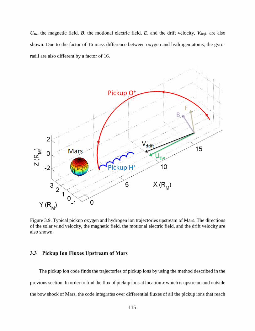
115

Usw, the magnetic field, B, the motional electric field, E, and the drift velocity, Vdrift, are also

shown. Due to the factor of 16 mass difference between oxygen and hydrogen atoms, the gyro-

radii are also different by a factor of 16.

Figure 3.9. Typical pickup oxygen and hydrogen ion trajectories upstream of Mars. The directions

of the solar wind velocity, the magnetic field, the motional electric field, and the drift velocity are

also shown.

3.3 Pickup Ion Fluxes Upstream of Mars

The pickup ion code finds the trajectories of pickup ions by using the method described in the

previous section. In order to find the flux of pickup ions at location x which is upstream and outside

the bow shock of Mars, the code integrates over differential fluxes of all the pickup ions that reach

116

point x. Therefore, the code finds the points on a curve on which pickup ions must be born in order

to reach point x by using the solutions to the equations of motion. The code divides this curve into

several elements with a configurable distance element and finds the fluxes of pickup ions using

the equation:

Pickup ion flux for species s = Is ∫ ns (x) dx, 3.36

where Is is the sum of all ionization frequencies, Is = IPI + ICX + IEI for species s (O or H), ns (x) is

the neutral density for species s at the mid-point of each distance element, and dx is the distance

element between two consecutive points on the “pickup ion birth curve”. Pickup ions born at each

point on this curve will reach the sampling point, x, at which the code calculates the pickup ion

flux. The code then bins these fluxes based on the energy and direction of the incidence of pickup

ions in order to simulate instrument measurements according to instrument specifications. Chapter

4 provides details on the SEP and SWIA instruments on MAVEN and includes model-data

comparison for pickup ion measurements made by each instrument.

The fluxes of pickup ions for several cases with different solar wind speeds, IMF strengths,

and θUB are provided below for both oxygen and hydrogen pickup ions. For these case studies, the

ionization frequency for both oxygen and hydrogen atoms is assumed to be 4.5 × 10-7 s-1. The

exospheric density profiles are adapted from Rahmati et al. [2014] for oxygen and from Feldman

et al. [2011] for hydrogen and displayed in Figure 3.1. The sampling point is located upstream of

Mars at an altitude of 6200 km, i.e. x = [RM + 6200 km, 0, 0], where RM = 3400 km is the radius

of Mars. This altitude is the furthest MAVEN can get upstream (apoapsis) during its 4.5-hour

elliptical orbit around Mars. Note that MAVEN’s orbit precesses with time and the apoapsis is not

always located outside the bow shock.

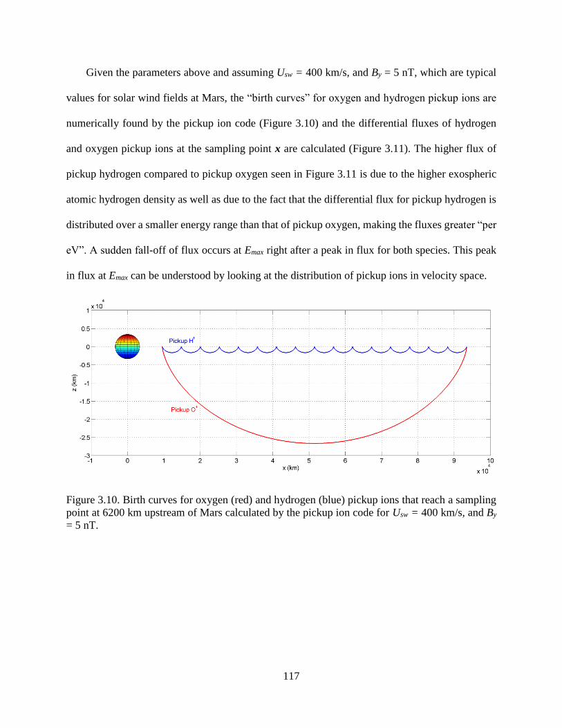
117

Given the parameters above and assuming Usw = 400 km/s, and By = 5 nT, which are typical

values for solar wind fields at Mars, the “birth curves” for oxygen and hydrogen pickup ions are

numerically found by the pickup ion code (Figure 3.10) and the differential fluxes of hydrogen

and oxygen pickup ions at the sampling point x are calculated (Figure 3.11). The higher flux of

pickup hydrogen compared to pickup oxygen seen in Figure 3.11 is due to the higher exospheric

atomic hydrogen density as well as due to the fact that the differential flux for pickup hydrogen is

distributed over a smaller energy range than that of pickup oxygen, making the fluxes greater “per

eV”. A sudden fall-off of flux occurs at Emax right after a peak in flux for both species. This peak

in flux at Emax can be understood by looking at the distribution of pickup ions in velocity space.

Figure 3.10. Birth curves for oxygen (red) and hydrogen (blue) pickup ions that reach a sampling

point at 6200 km upstream of Mars calculated by the pickup ion code for Usw = 400 km/s, and By

= 5 nT.

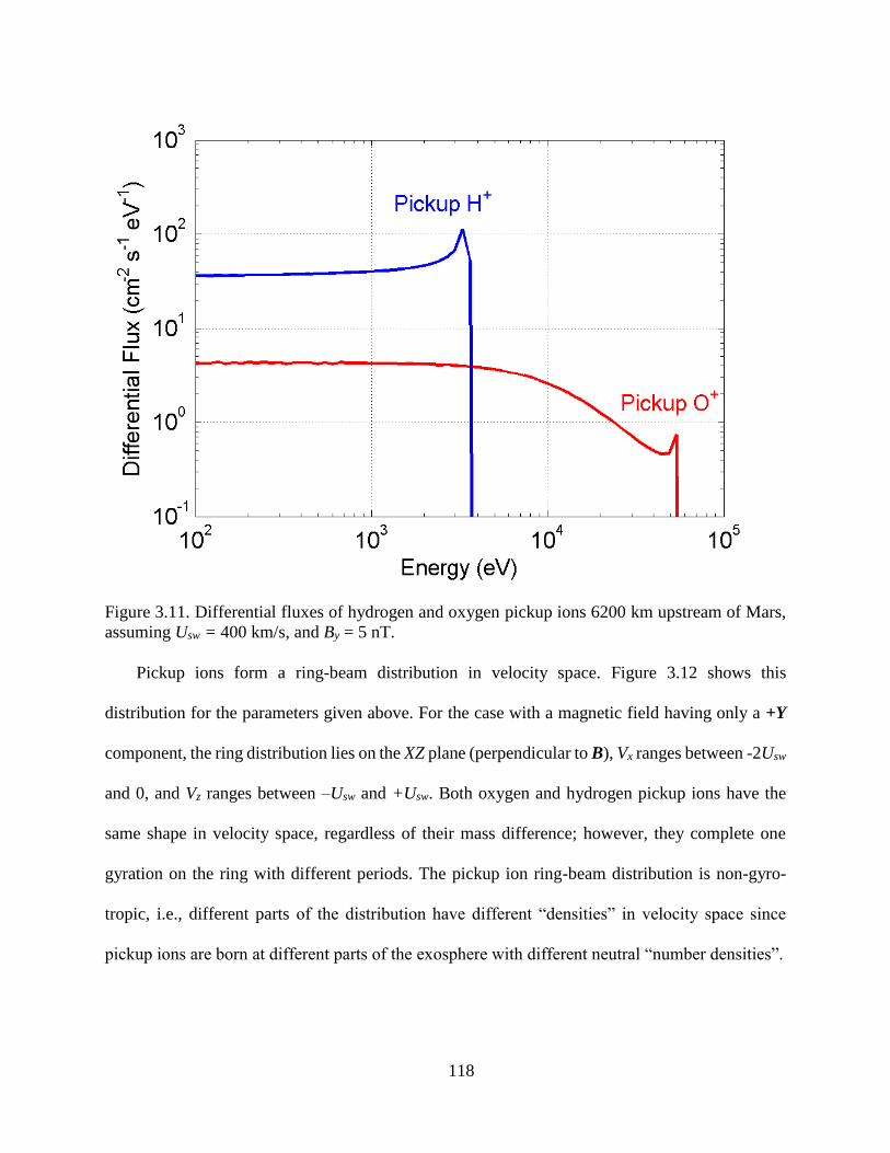
118

Figure 3.11. Differential fluxes of hydrogen and oxygen pickup ions 6200 km upstream of Mars,

assuming Usw = 400 km/s, and By = 5 nT.

Pickup ions form a ring-beam distribution in velocity space. Figure 3.12 shows this

distribution for the parameters given above. For the case with a magnetic field having only a +Y

component, the ring distribution lies on the XZ plane (perpendicular to B), Vx ranges between -2Usw

and 0, and Vz ranges between –Usw and +Usw. Both oxygen and hydrogen pickup ions have the

same shape in velocity space, regardless of their mass difference; however, they complete one

gyration on the ring with different periods. The pickup ion ring-beam distribution is non-gyro-

tropic, i.e., different parts of the distribution have different “densities” in velocity space since

pickup ions are born at different parts of the exosphere with different neutral “number densities”.

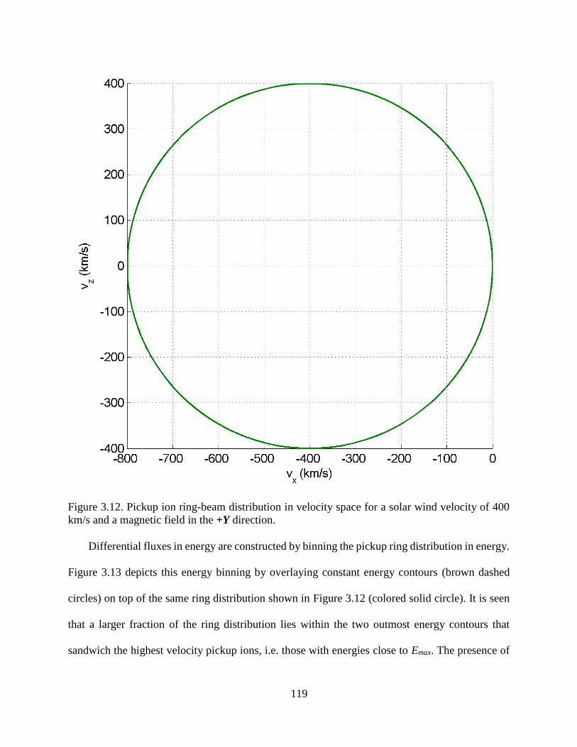
119

Figure 3.12. Pickup ion ring-beam distribution in velocity space for a solar wind velocity of 400

km/s and a magnetic field in the +Y direction.

Differential fluxes in energy are constructed by binning the pickup ring distribution in energy.

Figure 3.13 depicts this energy binning by overlaying constant energy contours (brown dashed

circles) on top of the same ring distribution shown in Figure 3.12 (colored solid circle). It is seen

that a larger fraction of the ring distribution lies within the two outmost energy contours that

sandwich the highest velocity pickup ions, i.e. those with energies close to Emax. The presence of

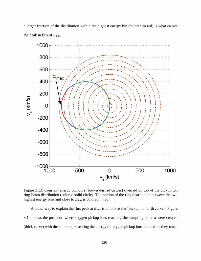
120

a larger fraction of the distribution within the highest energy bin (colored in red) is what causes

the peak in flux at Emax.

Figure 3.13. Constant energy contours (brown dashed circles) overlaid on top of the pickup ion

ring-beam distribution (colored solid circle). The portion of the ring distribution between the two

highest energy bins and close to Emax is colored in red.

Another way to explain the flux peak at Emax is to look at the “pickup ion birth curve”. Figure

3.14 shows the positions where oxygen pickup ions reaching the sampling point x were created

(thick curve) with the colors representing the energy of oxygen pickup ions at the time they reach

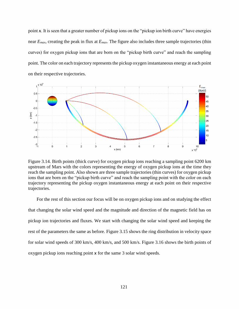
121

point x. It is seen that a greater number of pickup ions on the “pickup ion birth curve” have energies

near Emax, creating the peak in flux at Emax. The figure also includes three sample trajectories (thin

curves) for oxygen pickup ions that are born on the “pickup birth curve” and reach the sampling

point. The color on each trajectory represents the pickup oxygen instantaneous energy at each point

on their respective trajectories.

Figure 3.14. Birth points (thick curve) for oxygen pickup ions reaching a sampling point 6200 km

upstream of Mars with the colors representing the energy of oxygen pickup ions at the time they

reach the sampling point. Also shown are three sample trajectories (thin curves) for oxygen pickup

ions that are born on the “pickup birth curve” and reach the sampling point with the color on each

trajectory representing the pickup oxygen instantaneous energy at each point on their respective

trajectories.

For the rest of this section our focus will be on oxygen pickup ions and on studying the effect

that changing the solar wind speed and the magnitude and direction of the magnetic field has on

pickup ion trajectories and fluxes. We start with changing the solar wind speed and keeping the

rest of the parameters the same as before. Figure 3.15 shows the ring distribution in velocity space

for solar wind speeds of 300 km/s, 400 km/s, and 500 km/s. Figure 3.16 shows the birth points of

oxygen pickup ions reaching point x for the same 3 solar wind speeds.

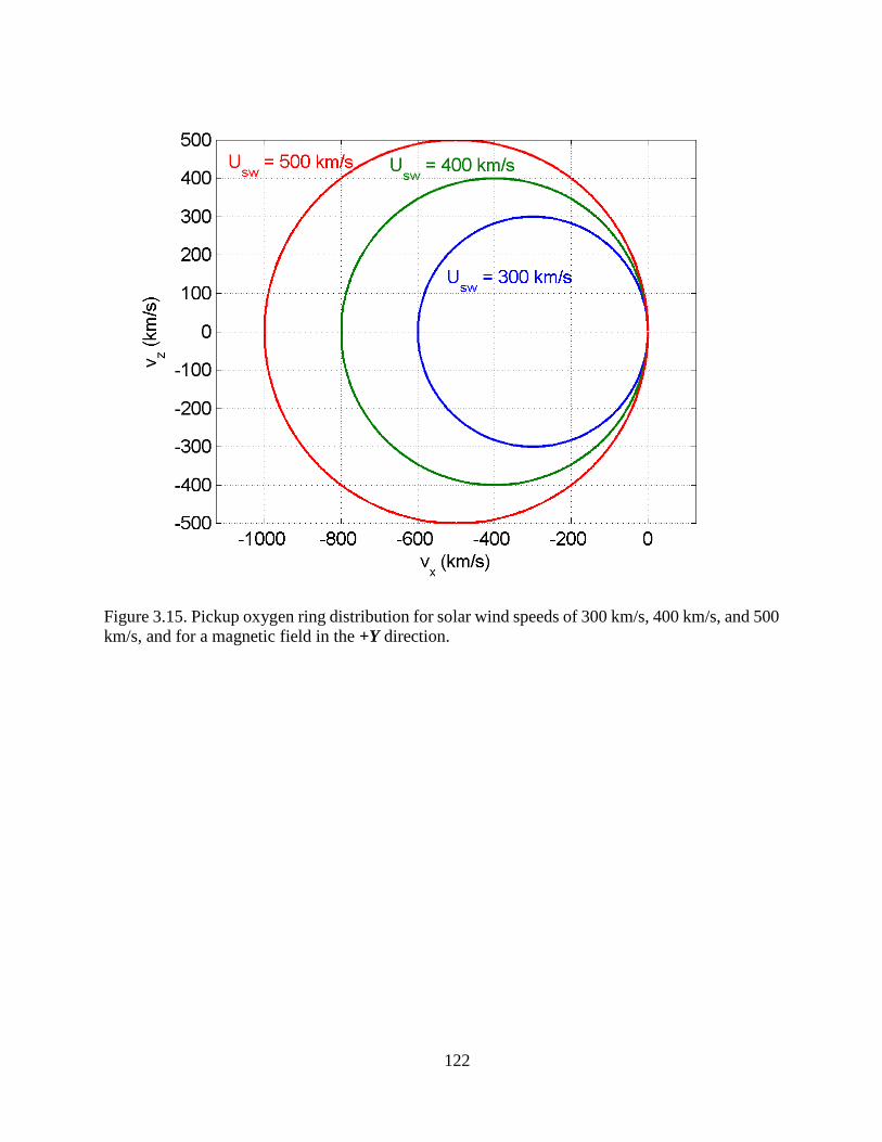
122

Figure 3.15. Pickup oxygen ring distribution for solar wind speeds of 300 km/s, 400 km/s, and 500

km/s, and for a magnetic field in the +Y direction.

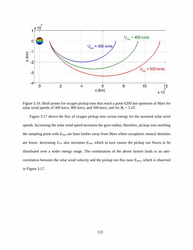
123

Figure 3.16. Birth points for oxygen pickup ions that reach a point 6200 km upstream of Mars for

solar wind speeds of 300 km/s, 400 km/s, and 500 km/s, and for By = 5 nT.

Figure 3.17 shows the flux of oxygen pickup ions versus energy for the assumed solar wind

speeds. Increasing the solar wind speed increases the gyro-radius; therefore, pickup ions reaching

the sampling point with Emax are born farther away from Mars where exospheric neutral densities

are lower. Increasing Usw also increases Emax which in turn causes the pickup ion fluxes to be

distributed over a wider energy range. The combination of the above factors leads to an anti-

correlation between the solar wind velocity and the pickup ion flux near Emax, which is observed

in Figure 3.17.

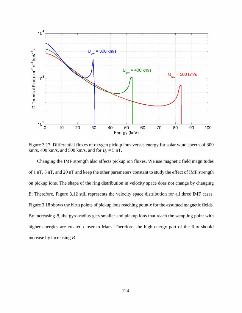
124

Figure 3.17. Differential fluxes of oxygen pickup ions versus energy for solar wind speeds of 300

km/s, 400 km/s, and 500 km/s, and for By = 5 nT.

Changing the IMF strength also affects pickup ion fluxes. We use magnetic field magnitudes

of 1 nT, 5 nT, and 20 nT and keep the other parameters constant to study the effect of IMF strength

on pickup ions. The shape of the ring distribution in velocity space does not change by changing

B; Therefore, Figure 3.12 still represents the velocity space distribution for all three IMF cases.

Figure 3.18 shows the birth points of pickup ions reaching point x for the assumed magnetic fields.

By increasing B, the gyro-radius gets smaller and pickup ions that reach the sampling point with

higher energies are created closer to Mars. Therefore, the high energy part of the flux should

increase by increasing B.

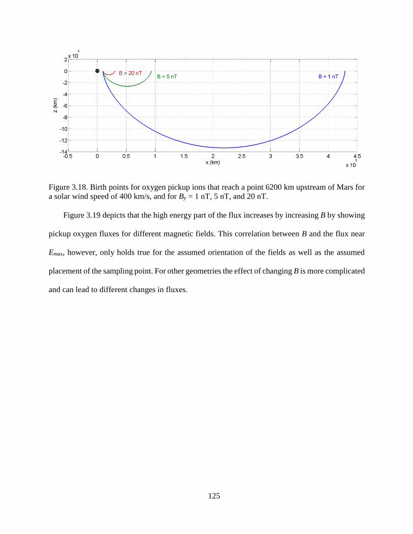
125


a solar wind speed of 400 km/s, and for By = 1 nT, 5 nT, and 20 nT.

Figure 3.19 depicts that the high energy part of the flux increases by increasing B by showing

pickup oxygen fluxes for different magnetic fields. This correlation between B and the flux near

Emax, however, only holds true for the assumed orientation of the fields as well as the assumed

placement of the sampling point. For other geometries the effect of changing B is more complicated

and can lead to different changes in fluxes.

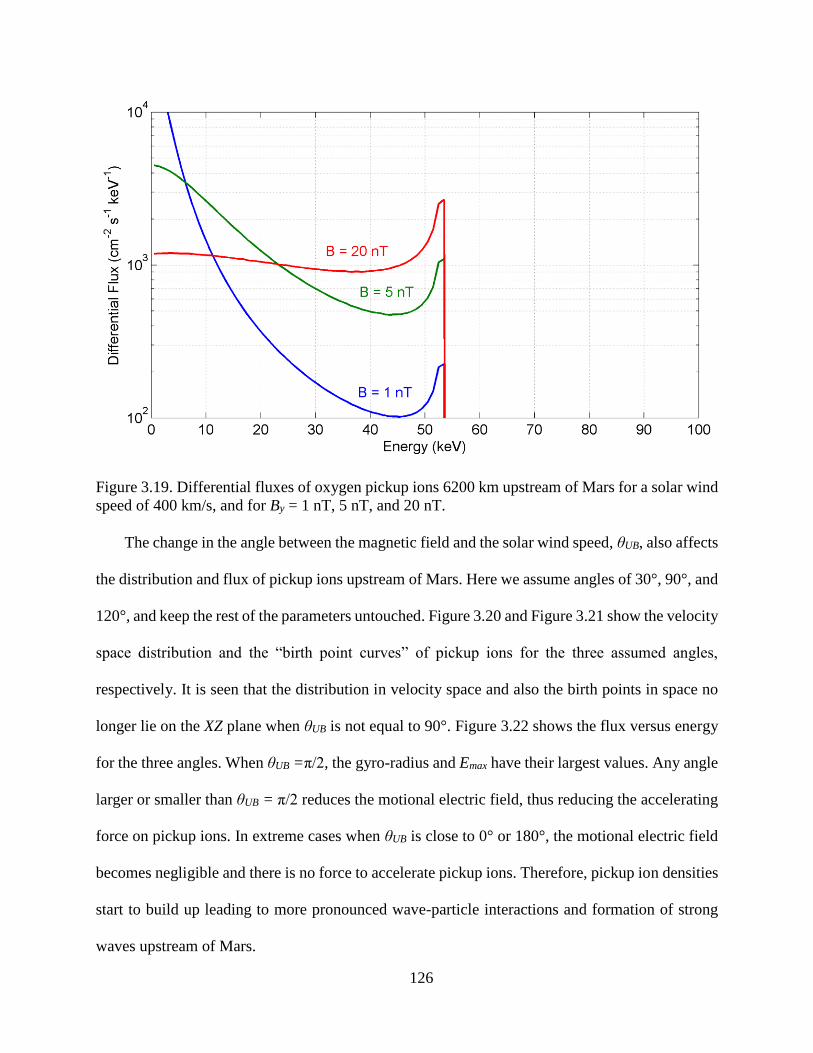
126

Figure 3.19. Differential fluxes of oxygen pickup ions 6200 km upstream of Mars for a solar wind

speed of 400 km/s, and for By = 1 nT, 5 nT, and 20 nT.

The change in the angle between the magnetic field and the solar wind speed, θUB, also affects

the distribution and flux of pickup ions upstream of Mars. Here we assume angles of 30°, 90°, and

120°, and keep the rest of the parameters untouched. Figure 3.20 and Figure 3.21 show the velocity

space distribution and the “birth point curves” of pickup ions for the three assumed angles,

respectively. It is seen that the distribution in velocity space and also the birth points in space no

longer lie on the XZ plane when θUB is not equal to 90°. Figure 3.22 shows the flux versus energy

for the three angles. When θUB =π/2, the gyro-radius and Emax have their largest values. Any angle

larger or smaller than θUB = π/2 reduces the motional electric field, thus reducing the accelerating

force on pickup ions. In extreme cases when θUB is close to 0° or 180°, the motional electric field

becomes negligible and there is no force to accelerate pickup ions. Therefore, pickup ion densities

start to build up leading to more pronounced wave-particle interactions and formation of strong

waves upstream of Mars.

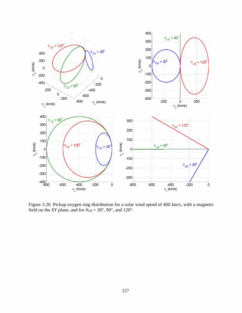
127

Figure 3.20. Pickup oxygen ring distribution for a solar wind speed of 400 km/s, with a magnetic

field on the XY plane, and for θUB = 30°, 90°, and 120°.

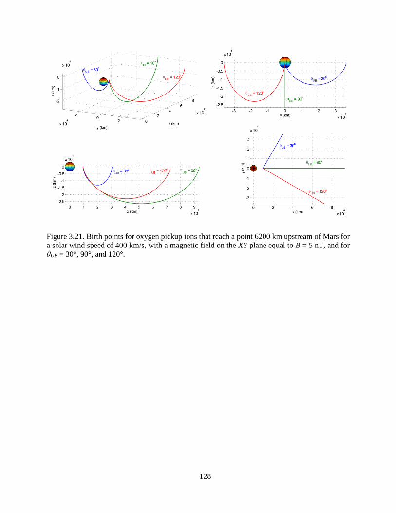
128


a solar wind speed of 400 km/s, with a magnetic field on the XY plane equal to B = 5 nT, and for

θUB = 30°, 90°, and 120°.

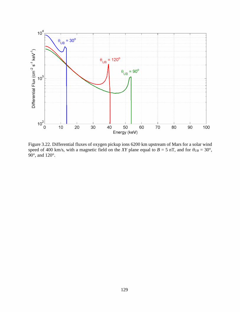
129

Figure 3.22. Differential fluxes of oxygen pickup ions 6200 km upstream of Mars for a solar wind

speed of 400 km/s, with a magnetic field on the XY plane equal to B = 5 nT, and for θUB = 30°,

90°, and 120°.

130

4 Pickup Ions Measured by MAVEN

The hot oxygen exosphere of Mars resembles a comet’s coma in that both are very extensive

[Cravens et al., 2002; Nagy et al., 2004]. A heavy ion (e.g., oxygen, water group) created in the

far upstream part of these extended media and picked up by the solar wind will have enough space

to reach the peak of its gyro-motion and obtain the maximum pickup energy [Coates, 2004].

Depending on solar wind conditions, this energy can be in excess of tens of keV. The Tunde-M

solid state detector on the VEGA-1 spacecraft detected water group pickup ions outside the bow

shock of comet Halley [Kecskemety et al., 1989]. The Ion and Electron Sensor (IES) onboard the

Rosetta spacecraft also detected water group pickup ions in the vicinity of comet 67P/Churyumov-

Gerasimenko [Goldstein et al., 2015].

The SLED (Solar Low-Energy Detector) solid state detector onboard the Phobos-2 spacecraft

made some initially puzzling measurements of energetic oxygen ions near Mars not associated

with any solar or solar wind event [McKenna-Lawlor et al., 1993]. Cravens et al. [2002] suggested

that ionization of exospheric oxygen creates pickup ions, far upstream of the bow-shock, that are

sufficiently energetic near the planet (and spacecraft) to be detected by the solid state SLED

detectors. Their quantitative model-data comparisons indicated that neutral O densities of 7 cm-3

at about 10 RM upstream of Mars would be consistent with SLED’s O+ flux measurements.

Since MAVEN’s arrival at Mars, the SEP (Solar Energetic Particle) and SWIA (Solar Wind

Ion Analyzer) instruments have been detecting pickup ions outside the bow shock of Mars. These

pickup ions are associated with the exospheric neutral oxygen and hydrogen atoms. MAVEN SEP

can detect oxygen pickup ions with energies above ~60 keV, but is blind to hydrogen pickup ions.

131

SWIA can measure both oxygen and hydrogen pickup ions with a maximum energy of 25 keV. In

this chapter measured pickup ion data from the SEP and SWIA instruments are shown and

compared to modeled pickup ion fluxes. The model used to simulate pickup ions upstream of Mars

is explained in Chapter 3. These model-data comparisons give us insight into the processes

populating the exosphere of Mars and can be used to validate models of the Martian exosphere.

4.1 MAVEN SEP

One of the science goals of MAVEN is to study how Mars’s upper atmosphere responds to

the drivers of atmospheric escape. An important driver is energetic particles from the Sun that hit

Mars during solar storms. These particle events are due to solar flares and Coronal Mass Ejections

(CME’s) that occur several times a year. They peak during the maximum phase of the 11-year

solar cycle and can have significant impact on the atmosphere of Mars. The SEP instrument on

MAVEN measures the flux of these energetic particles at Mars using telescopic solid state

detectors [Larson et al., 2015]. High energy particle observations made by SEP can be used to

determine the effects of energy deposition in the Martian upper atmosphere, and quantify the role

of solar particle events in atmospheric escape from Mars. SEP can also detect energetic oxygen

pickup ions that are accelerated by the solar wind motional electric field upstream of Mars

[Rahmati et al., 2014,2015].

There are two SEP sensors mounted on MAVEN, each containing two double-ended

telescopes that have perpendicular look directions. Figure 4.1 shows the placement of each SEP as

well as each individual look direction. Each one of the four telescopes consists of a stack of three

silicon detectors that detect primarily ions at one end (called “open,” where a strong magnet sweeps

132

away electrons below ~250 keV) and electrons in the other end (called “foil,” where a thin foil

stops ions below ~250 keV). A third silicon layer (called “thick”), in the middle of the open and

the foil detectors, is used to detect the highest energy ions/electrons that penetrate the open/foil

detector [Larson et al., 2015]. Figure 4.2 shows a schematic of the electron and ion telescopes.

Oxygen pickup ions are detected in the open detectors that have a look direction in the sunward

hemisphere; therefore, in the model-data comparisons, only data from the two open “Front”

detectors (namely SEP1F and SEP2F) are presented.

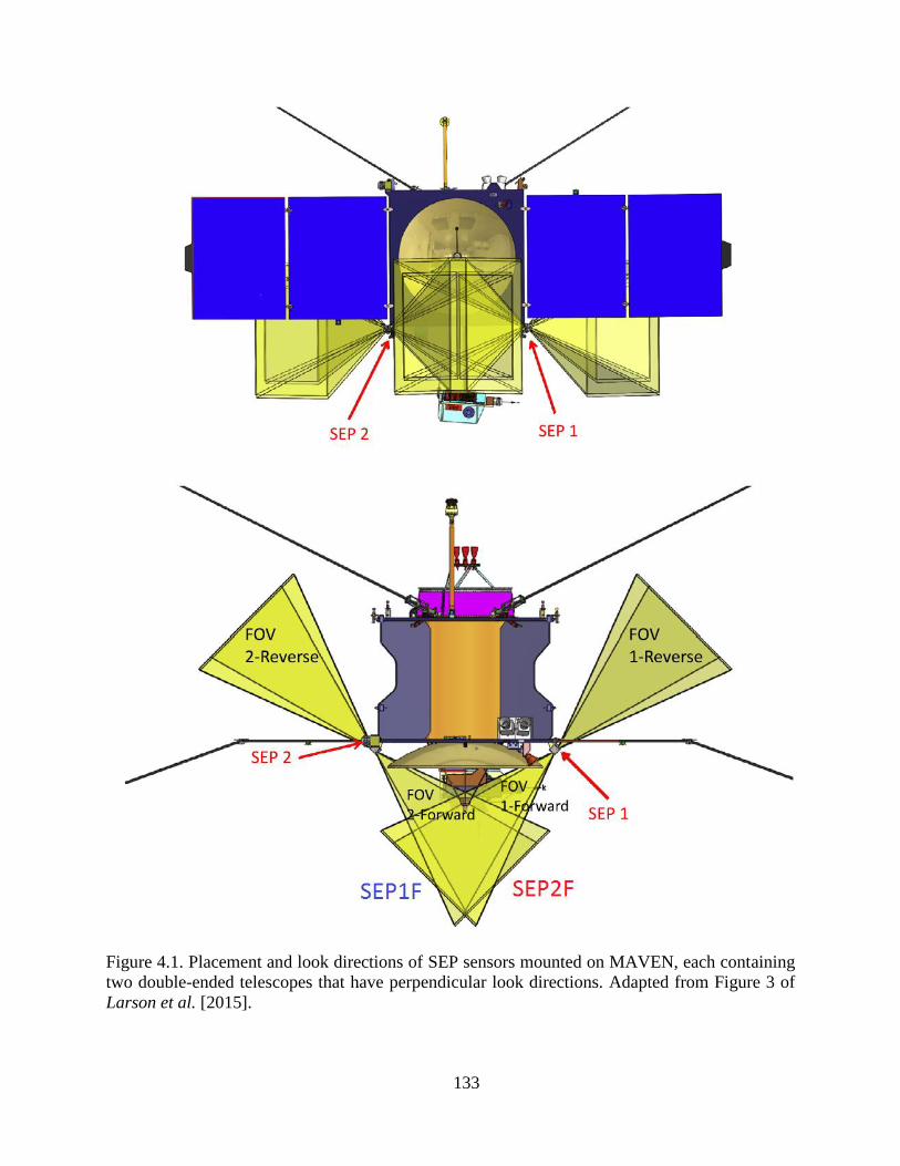
133

Figure 4.1. Placement and look directions of SEP sensors mounted on MAVEN, each containing

two double-ended telescopes that have perpendicular look directions. Adapted from Figure 3 of

Larson et al. [2015].

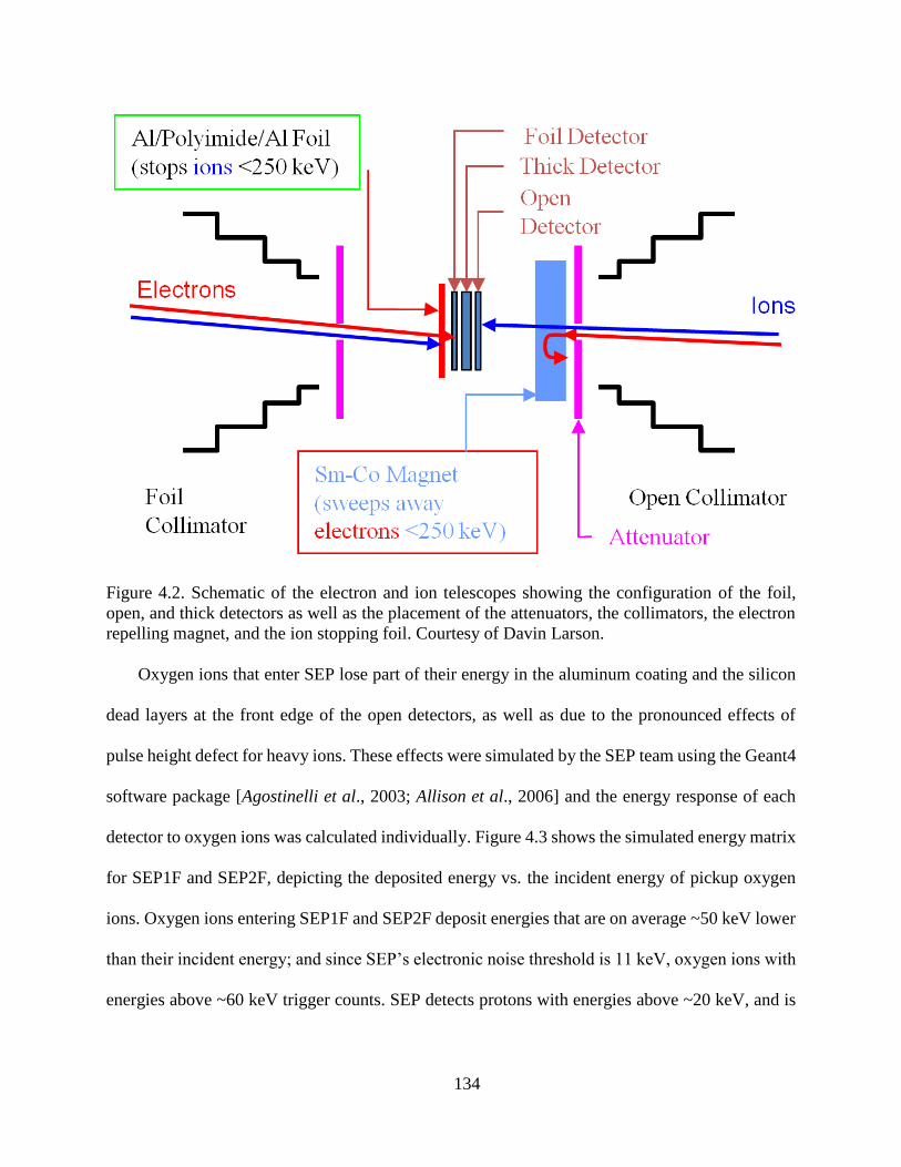
134

Figure 4.2. Schematic of the electron and ion telescopes showing the configuration of the foil,

open, and thick detectors as well as the placement of the attenuators, the collimators, the electron

repelling magnet, and the ion stopping foil. Courtesy of Davin Larson.

Oxygen ions that enter SEP lose part of their energy in the aluminum coating and the silicon

dead layers at the front edge of the open detectors, as well as due to the pronounced effects of

pulse height defect for heavy ions. These effects were simulated by the SEP team using the Geant4

software package [Agostinelli et al., 2003; Allison et al., 2006] and the energy response of each

detector to oxygen ions was calculated individually. Figure 4.3 shows the simulated energy matrix

for SEP1F and SEP2F, depicting the deposited energy vs. the incident energy of pickup oxygen

ions. Oxygen ions entering SEP1F and SEP2F deposit energies that are on average ~50 keV lower

than their incident energy; and since SEP’s electronic noise threshold is 11 keV, oxygen ions with

energies above ~60 keV trigger counts. SEP detects protons with energies above ~20 keV, and is

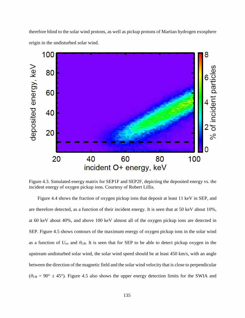
135

therefore blind to the solar wind protons, as well as pickup protons of Martian hydrogen exosphere

origin in the undisturbed solar wind.

Figure 4.3. Simulated energy matrix for SEP1F and SEP2F, depicting the deposited energy vs. the

incident energy of oxygen pickup ions. Courtesy of Robert Lillis.

Figure 4.4 shows the fraction of oxygen pickup ions that deposit at least 11 keV in SEP, and

are therefore detected, as a function of their incident energy. It is seen that at 50 keV about 10%,

at 60 keV about 40%, and above 100 keV almost all of the oxygen pickup ions are detected in

SEP. Figure 4.5 shows contours of the maximum energy of oxygen pickup ions in the solar wind

as a function of Usw and θUB. It is seen that for SEP to be able to detect pickup oxygen in the

upstream undisturbed solar wind, the solar wind speed should be at least 450 km/s, with an angle

between the direction of the magnetic field and the solar wind velocity that is close to perpendicular

(θUB = 90° ± 45°). Figure 4.5 also shows the upper energy detection limits for the SWIA and

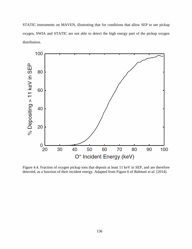
136

STATIC instruments on MAVEN, illustrating that for conditions that allow SEP to see pickup

oxygen, SWIA and STATIC are not able to detect the high energy part of the pickup oxygen

distribution.

Figure 4.4. Fraction of oxygen pickup ions that deposit at least 11 keV in SEP, and are therefore

detected, as a function of their incident energy. Adapted from Figure 6 of Rahmati et al. [2014].

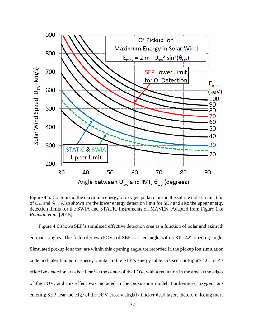
137

Figure 4.5. Contours of the maximum energy of oxygen pickup ions in the solar wind as a function

of Usw and θUB. Also shown are the lower energy detection limit for SEP and also the upper energy

detection limits for the SWIA and STATIC instruments on MAVEN. Adapted from Figure 1 of


Figure 4.6 shows SEP’s simulated effective detection area as a function of polar and azimuth

entrance angles. The field of view (FOV) of SEP is a rectangle with a 31°×42° opening angle.

Simulated pickup ions that are within this opening angle are recorded in the pickup ion simulation

code and later binned in energy similar to the SEP’s energy table. As seen in Figure 4.6, SEP’s

effective detection area is ~1 cm2 at the center of the FOV, with a reduction in the area at the edges

of the FOV, and this effect was included in the pickup ion model. Furthermore, oxygen ions

entering SEP near the edge of the FOV cross a slightly thicker dead layer; therefore, losing more

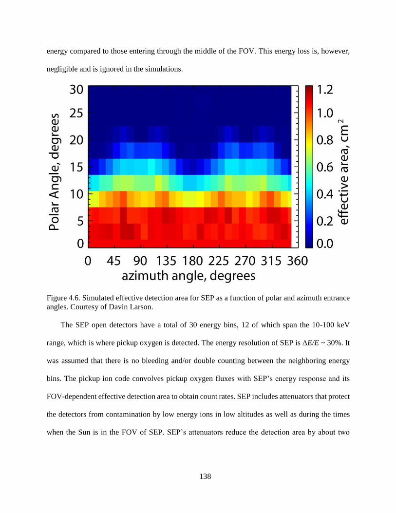
138

energy compared to those entering through the middle of the FOV. This energy loss is, however,

negligible and is ignored in the simulations.

Figure 4.6. Simulated effective detection area for SEP as a function of polar and azimuth entrance

angles. Courtesy of Davin Larson.

The SEP open detectors have a total of 30 energy bins, 12 of which span the 10-100 keV

range, which is where pickup oxygen is detected. The energy resolution of SEP is ΔE/E ~ 30%. It

was assumed that there is no bleeding and/or double counting between the neighboring energy

bins. The pickup ion code convolves pickup oxygen fluxes with SEP’s energy response and its

FOV-dependent effective detection area to obtain count rates. SEP includes attenuators that protect

the detectors from contamination by low energy ions in low altitudes as well as during the times

when the Sun is in the FOV of SEP. SEP’s attenuators reduce the detection area by about two

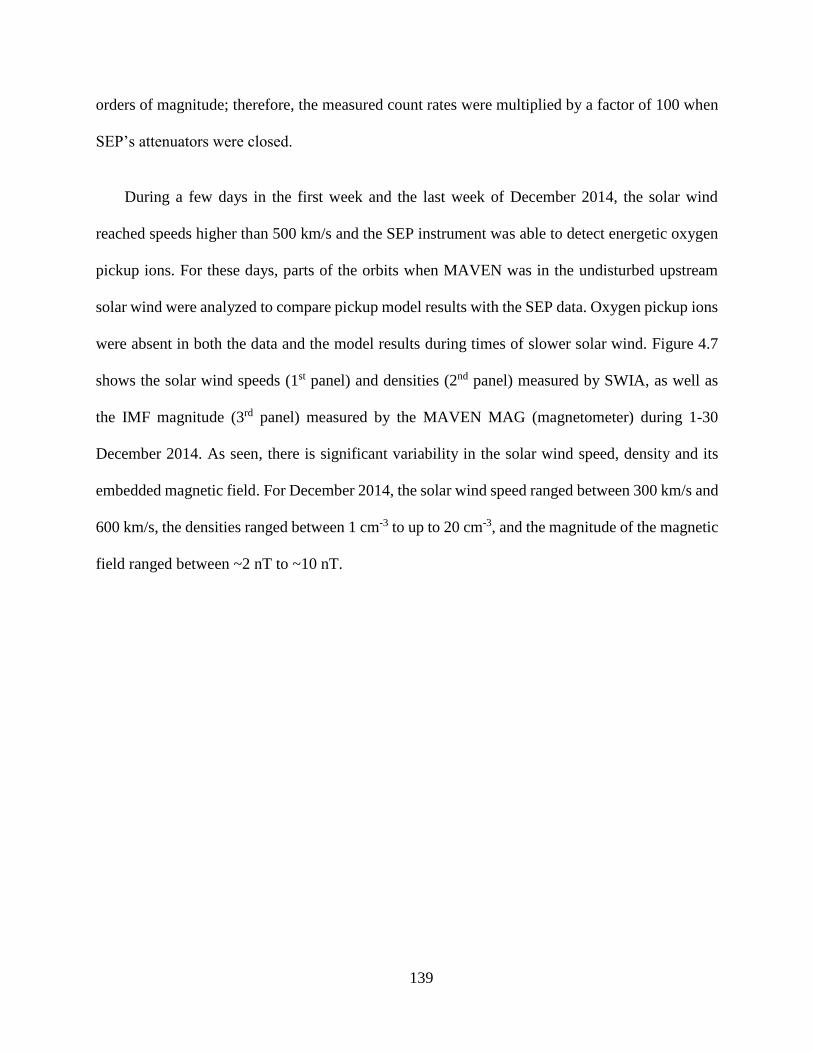
139

orders of magnitude; therefore, the measured count rates were multiplied by a factor of 100 when

SEP’s attenuators were closed.

During a few days in the first week and the last week of December 2014, the solar wind

reached speeds higher than 500 km/s and the SEP instrument was able to detect energetic oxygen

pickup ions. For these days, parts of the orbits when MAVEN was in the undisturbed upstream

solar wind were analyzed to compare pickup model results with the SEP data. Oxygen pickup ions

were absent in both the data and the model results during times of slower solar wind. Figure 4.7

shows the solar wind speeds (1st panel) and densities (2nd panel) measured by SWIA, as well as

the IMF magnitude (3rd panel) measured by the MAVEN MAG (magnetometer) during 1-30

December 2014. As seen, there is significant variability in the solar wind speed, density and its

embedded magnetic field. For December 2014, the solar wind speed ranged between 300 km/s and

600 km/s, the densities ranged between 1 cm-3 to up to 20 cm-3, and the magnitude of the magnetic

field ranged between ~2 nT to ~10 nT.

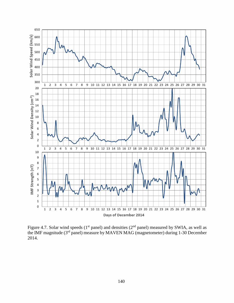
140

Figure 4.7. Solar wind speeds (1st panel) and densities (2nd panel) measured by SWIA, as well as

the IMF magnitude (3rd panel) measure by MAVEN MAG (magnetometer) during 1-30 December

2014.

141

4.1.1 Orbit 343

Figure 4.8 shows a 1-hour time period of orbit 343 starting at 14:30 UTC on 2 December

2014, when the solar wind speed was ~525 km/s. Panel (a) shows the three components of the IMF

measured by MAVEN MAG in MSO (Mars-Solar-Orbital) coordinates, panel (b) shows the

calculated angle between the solar wind velocity and the magnetic field, and panel (c) shows the

maximum energy that oxygen pickup ions can achieve (Emax). The SEP measured and modeled

pickup oxygen spectrograms for SEP2F are presented in panels (d) and (e), respectively. The

pickup ion code, as described in Chapter 3, takes in the parameters needed for calculating the flux

of pickup ions and simulates SEP’s measurements.

Figure 4.8. Model-data comparison of SEP-detected oxygen pickup ions for part of orbit 343. The

panels are described in the text. Adapted from Figure 3 of Rahmati et al. [2015].

A good agreement is found between the model results and the data, confirming detection of

pickup oxygen associated with the Martian extended hot oxygen exosphere. In particular, the

fluctuations in the maximum energy calculated in panel (c) can be observed in both the data and

model results. For the whole time period shown in Figure 4.8, SEP2F was looking in the sunward

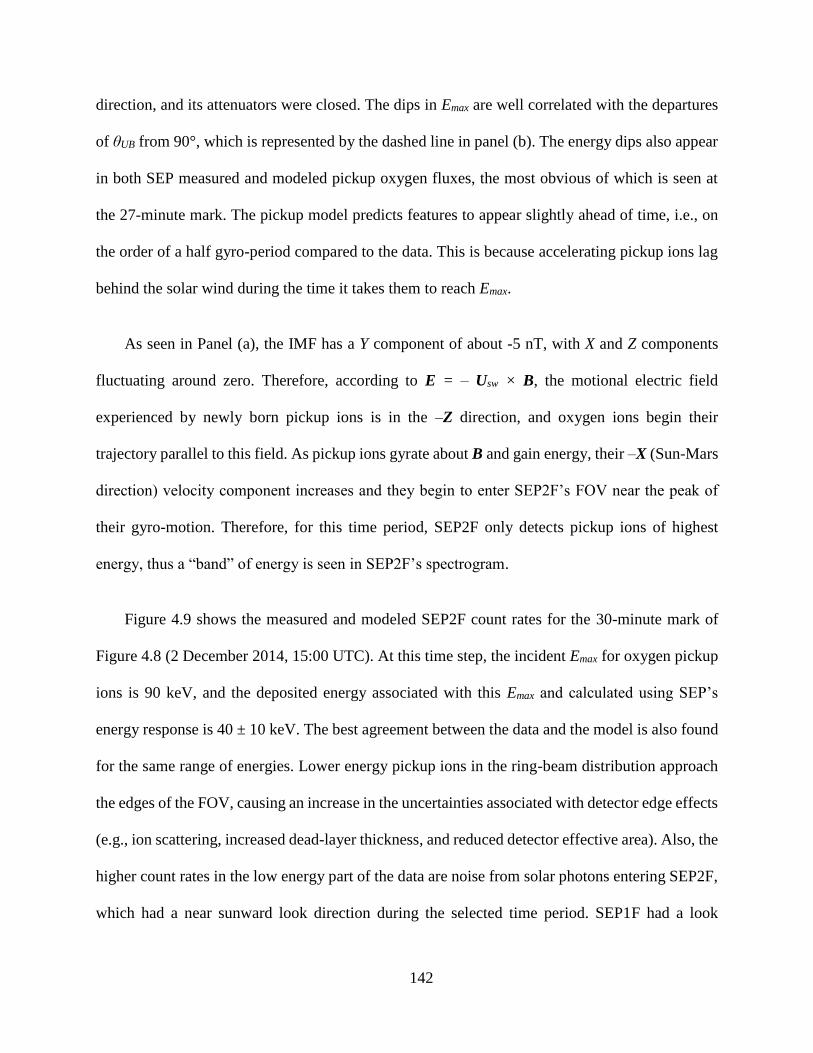
142

direction, and its attenuators were closed. The dips in Emax are well correlated with the departures

of θUB from 90°, which is represented by the dashed line in panel (b). The energy dips also appear

in both SEP measured and modeled pickup oxygen fluxes, the most obvious of which is seen at

the 27-minute mark. The pickup model predicts features to appear slightly ahead of time, i.e., on

the order of a half gyro-period compared to the data. This is because accelerating pickup ions lag

behind the solar wind during the time it takes them to reach Emax.

As seen in Panel (a), the IMF has a Y component of about -5 nT, with X and Z components

fluctuating around zero. Therefore, according to E = – Usw × B, the motional electric field

experienced by newly born pickup ions is in the –Z direction, and oxygen ions begin their

trajectory parallel to this field. As pickup ions gyrate about B and gain energy, their –X (Sun-Mars

direction) velocity component increases and they begin to enter SEP2F’s FOV near the peak of

their gyro-motion. Therefore, for this time period, SEP2F only detects pickup ions of highest

energy, thus a “band” of energy is seen in SEP2F’s spectrogram.

Figure 4.9 shows the measured and modeled SEP2F count rates for the 30-minute mark of

Figure 4.8 (2 December 2014, 15:00 UTC). At this time step, the incident Emax for oxygen pickup

ions is 90 keV, and the deposited energy associated with this Emax and calculated using SEP’s

energy response is 40 ± 10 keV. The best agreement between the data and the model is also found

for the same range of energies. Lower energy pickup ions in the ring-beam distribution approach

the edges of the FOV, causing an increase in the uncertainties associated with detector edge effects

(e.g., ion scattering, increased dead-layer thickness, and reduced detector effective area). Also, the

higher count rates in the low energy part of the data are noise from solar photons entering SEP2F,

which had a near sunward look direction during the selected time period. SEP1F had a look

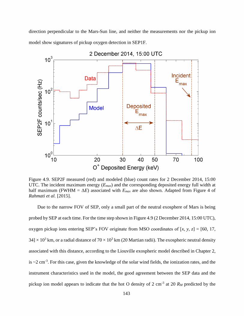
143

direction perpendicular to the Mars-Sun line, and neither the measurements nor the pickup ion

model show signatures of pickup oxygen detection in SEP1F.

Figure 4.9. SEP2F measured (red) and modeled (blue) count rates for 2 December 2014, 15:00

UTC. The incident maximum energy (Emax) and the corresponding deposited energy full width at

half maximum (FWHM = ΔE) associated with Emax are also shown. Adapted from Figure 4 of


Due to the narrow FOV of SEP, only a small part of the neutral exosphere of Mars is being

probed by SEP at each time. For the time step shown in Figure 4.9 (2 December 2014, 15:00 UTC),

oxygen pickup ions entering SEP’s FOV originate from MSO coordinates of [x, y, z] = [60, 17,

34] × 103 km, or a radial distance of 70 × 103 km (20 Martian radii). The exospheric neutral density

associated with this distance, according to the Liouville exospheric model described in Chapter 2,

is ~2 cm-3. For this case, given the knowledge of the solar wind fields, the ionization rates, and the

instrument characteristics used in the model, the good agreement between the SEP data and the

pickup ion model appears to indicate that the hot O density of 2 cm-3 at 20 RM predicted by the

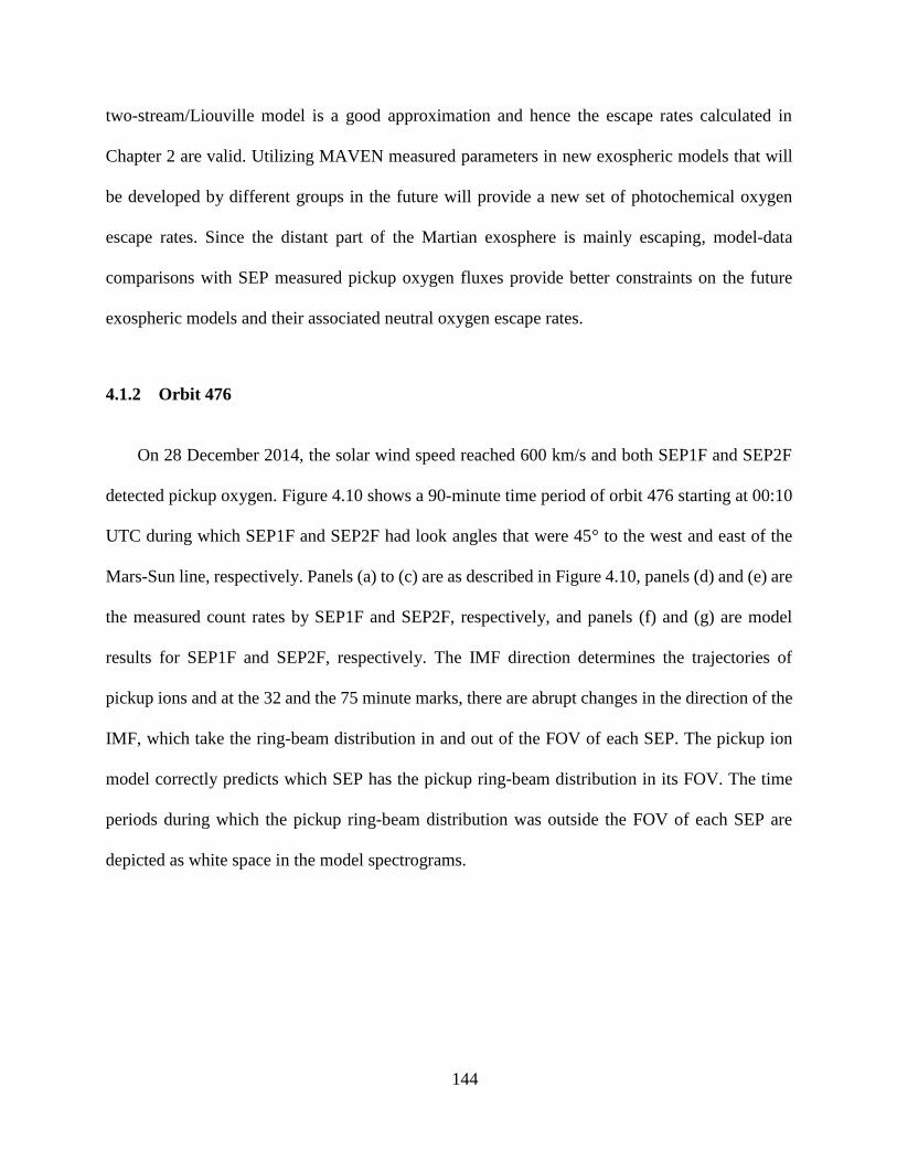
144

two-stream/Liouville model is a good approximation and hence the escape rates calculated in

Chapter 2 are valid. Utilizing MAVEN measured parameters in new exospheric models that will

be developed by different groups in the future will provide a new set of photochemical oxygen

escape rates. Since the distant part of the Martian exosphere is mainly escaping, model-data

comparisons with SEP measured pickup oxygen fluxes provide better constraints on the future

exospheric models and their associated neutral oxygen escape rates.

4.1.2 Orbit 476

On 28 December 2014, the solar wind speed reached 600 km/s and both SEP1F and SEP2F

detected pickup oxygen. Figure 4.10 shows a 90-minute time period of orbit 476 starting at 00:10

UTC during which SEP1F and SEP2F had look angles that were 45° to the west and east of the

Mars-Sun line, respectively. Panels (a) to (c) are as described in Figure 4.10, panels (d) and (e) are

the measured count rates by SEP1F and SEP2F, respectively, and panels (f) and (g) are model

results for SEP1F and SEP2F, respectively. The IMF direction determines the trajectories of

pickup ions and at the 32 and the 75 minute marks, there are abrupt changes in the direction of the

IMF, which take the ring-beam distribution in and out of the FOV of each SEP. The pickup ion

model correctly predicts which SEP has the pickup ring-beam distribution in its FOV. The time

periods during which the pickup ring-beam distribution was outside the FOV of each SEP are

depicted as white space in the model spectrograms.

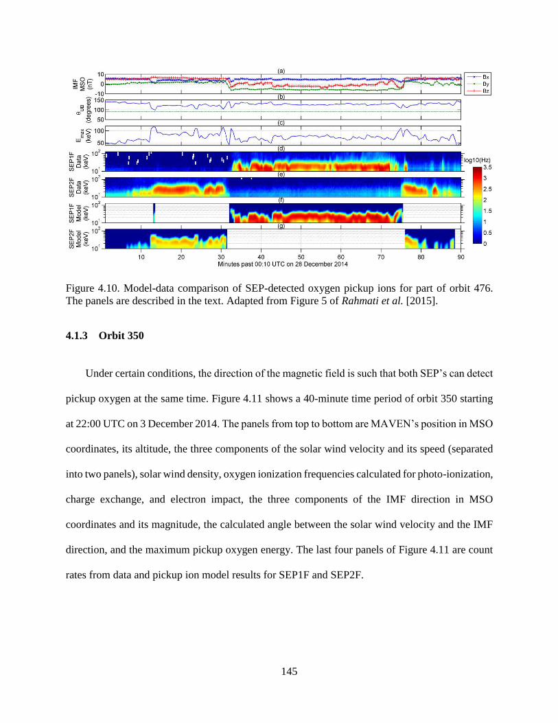
145


The panels are described in the text. Adapted from Figure 5 of Rahmati et al. [2015].

4.1.3 Orbit 350

Under certain conditions, the direction of the magnetic field is such that both SEP’s can detect

pickup oxygen at the same time. Figure 4.11 shows a 40-minute time period of orbit 350 starting

at 22:00 UTC on 3 December 2014. The panels from top to bottom are MAVEN’s position in MSO

coordinates, its altitude, the three components of the solar wind velocity and its speed (separated

into two panels), solar wind density, oxygen ionization frequencies calculated for photo-ionization,

charge exchange, and electron impact, the three components of the IMF direction in MSO

coordinates and its magnitude, the calculated angle between the solar wind velocity and the IMF

direction, and the maximum pickup oxygen energy. The last four panels of Figure 4.11 are count

rates from data and pickup ion model results for SEP1F and SEP2F.

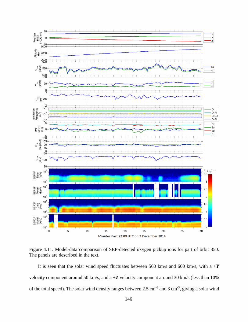
146


The panels are described in the text.

It is seen that the solar wind speed fluctuates between 560 km/s and 600 km/s, with a +Y

velocity component around 50 km/s, and a +Z velocity component around 30 km/s (less than 10%

of the total speed). The solar wind density ranges between 2.5 cm-3 and 3 cm-3, giving a solar wind

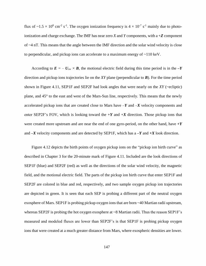
147

flux of ~1.5 × 108 cm-2 s-1. The oxygen ionization frequency is 4 × 10-7 s-1 mainly due to photo-

ionization and charge exchange. The IMF has near zero X and Y components, with a +Z component

of ~4 nT. This means that the angle between the IMF direction and the solar wind velocity is close

to perpendicular, and pickup ions can accelerate to a maximum energy of ~110 keV.

According to E = – Usw × B, the motional electric field during this time period is in the –Y

direction and pickup ions trajectories lie on the XY plane (perpendicular to B). For the time period

shown in Figure 4.11, SEP1F and SEP2F had look angles that were nearly on the XY (~ecliptic)

plane, and 45° to the east and west of the Mars-Sun line, respectively. This means that the newly

accelerated pickup ions that are created close to Mars have –Y and –X velocity components and

enter SEP2F’s FOV, which is looking toward the +Y and +X direction. Those pickup ions that

were created more upstream and are near the end of one gyro-period, on the other hand, have +Y

and –X velocity components and are detected by SEP1F, which has a –Y and +X look direction.

Figure 4.12 depicts the birth points of oxygen pickup ions on the “pickup ion birth curve” as

described in Chapter 3 for the 20-minute mark of Figure 4.11. Included are the look directions of

SEP1F (blue) and SEP2F (red) as well as the directions of the solar wind velocity, the magnetic

field, and the motional electric field. The parts of the pickup ion birth curve that enter SEP1F and

SEP2F are colored in blue and red, respectively, and two sample oxygen pickup ion trajectories

are depicted in green. It is seen that each SEP is probing a different part of the neutral oxygen

exosphere of Mars. SEP1F is probing pickup oxygen ions that are born ~40 Martian radii upstream,

whereas SEP2F is probing the hot oxygen exosphere at ~8 Martian radii. Thus the reason SEP1F’s

measured and modeled fluxes are lower than SEP2F’s is that SEP1F is probing pickup oxygen

ions that were created at a much greater distance from Mars, where exospheric densities are lower.

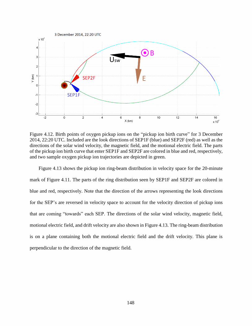
148

Figure 4.12. Birth points of oxygen pickup ions on the “pickup ion birth curve” for 3 December

2014, 22:20 UTC. Included are the look directions of SEP1F (blue) and SEP2F (red) as well as the

directions of the solar wind velocity, the magnetic field, and the motional electric field. The parts

of the pickup ion birth curve that enter SEP1F and SEP2F are colored in blue and red, respectively,

and two sample oxygen pickup ion trajectories are depicted in green.

Figure 4.13 shows the pickup ion ring-beam distribution in velocity space for the 20-minute

mark of Figure 4.11. The parts of the ring distribution seen by SEP1F and SEP2F are colored in

blue and red, respectively. Note that the direction of the arrows representing the look directions

for the SEP’s are reversed in velocity space to account for the velocity direction of pickup ions

that are coming “towards” each SEP. The directions of the solar wind velocity, magnetic field,

motional electric field, and drift velocity are also shown in Figure 4.13. The ring-beam distribution

is on a plane containing both the motional electric field and the drift velocity. This plane is

perpendicular to the direction of the magnetic field.

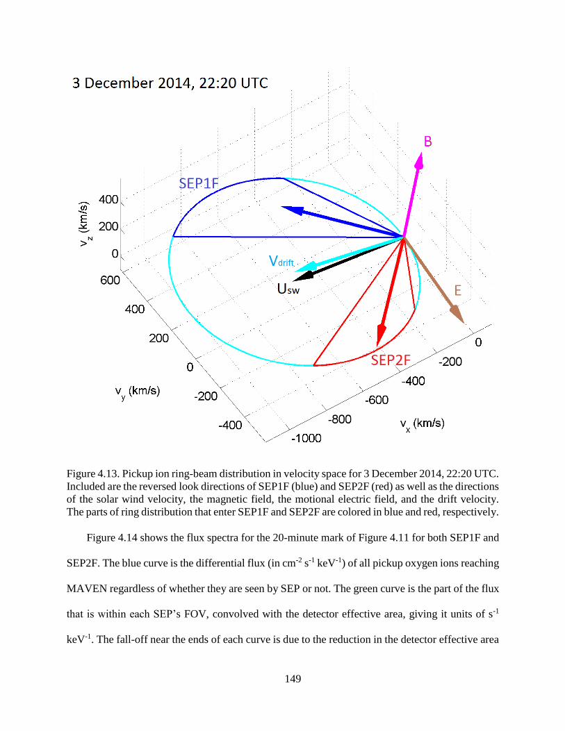
149

Figure 4.13. Pickup ion ring-beam distribution in velocity space for 3 December 2014, 22:20 UTC.

Included are the reversed look directions of SEP1F (blue) and SEP2F (red) as well as the directions

of the solar wind velocity, the magnetic field, the motional electric field, and the drift velocity.

The parts of ring distribution that enter SEP1F and SEP2F are colored in blue and red, respectively.

Figure 4.14 shows the flux spectra for the 20-minute mark of Figure 4.11 for both SEP1F and

SEP2F. The blue curve is the differential flux (in cm-2 s-1 keV-1) of all pickup oxygen ions reaching

MAVEN regardless of whether they are seen by SEP or not. The green curve is the part of the flux

that is within each SEP’s FOV, convolved with the detector effective area, giving it units of s-1

keV-1. The fall-off near the ends of each curve is due to the reduction in the detector effective area

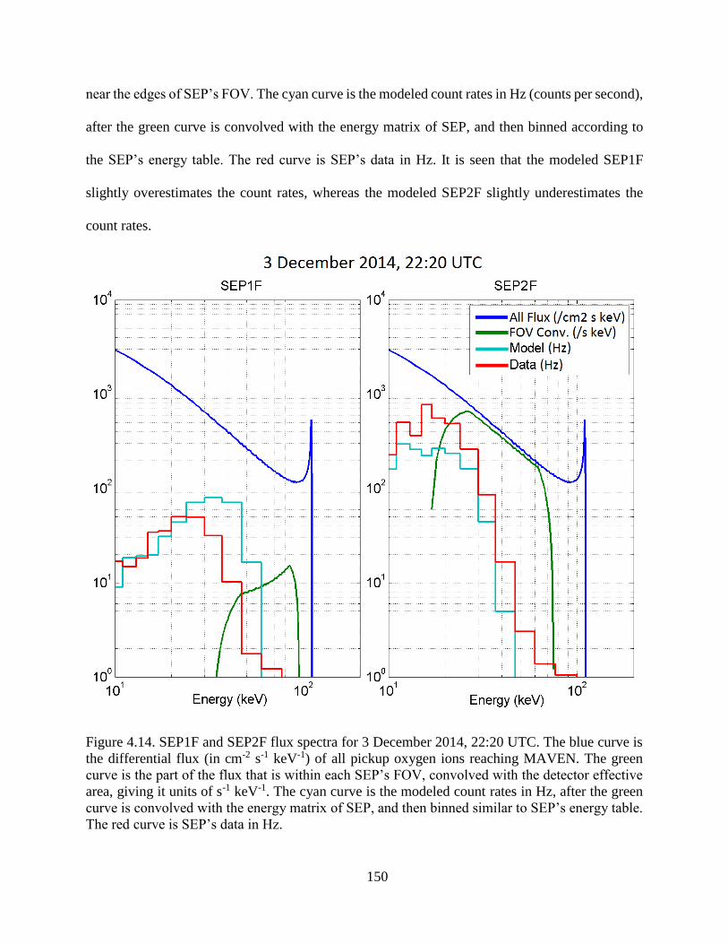
150

near the edges of SEP’s FOV. The cyan curve is the modeled count rates in Hz (counts per second),

after the green curve is convolved with the energy matrix of SEP, and then binned according to

the SEP’s energy table. The red curve is SEP’s data in Hz. It is seen that the modeled SEP1F

slightly overestimates the count rates, whereas the modeled SEP2F slightly underestimates the

count rates.

Figure 4.14. SEP1F and SEP2F flux spectra for 3 December 2014, 22:20 UTC. The blue curve is

the differential flux (in cm-2 s-1 keV-1) of all pickup oxygen ions reaching MAVEN. The green

curve is the part of the flux that is within each SEP’s FOV, convolved with the detector effective

area, giving it units of s-1 keV-1. The cyan curve is the modeled count rates in Hz, after the green

curve is convolved with the energy matrix of SEP, and then binned similar to SEP’s energy table.

The red curve is SEP’s data in Hz.

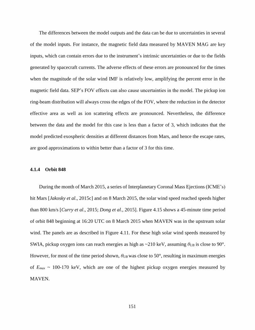
151

The differences between the model outputs and the data can be due to uncertainties in several

of the model inputs. For instance, the magnetic field data measured by MAVEN MAG are key

inputs, which can contain errors due to the instrument’s intrinsic uncertainties or due to the fields

generated by spacecraft currents. The adverse effects of these errors are pronounced for the times

when the magnitude of the solar wind IMF is relatively low, amplifying the percent error in the

magnetic field data. SEP’s FOV effects can also cause uncertainties in the model. The pickup ion

ring-beam distribution will always cross the edges of the FOV, where the reduction in the detector

effective area as well as ion scattering effects are pronounced. Nevertheless, the difference

between the data and the model for this case is less than a factor of 3, which indicates that the

model predicted exospheric densities at different distances from Mars, and hence the escape rates,

are good approximations to within better than a factor of 3 for this time.

4.1.4 Orbit 848

During the month of March 2015, a series of Interplanetary Coronal Mass Ejections (ICME’s)

hit Mars [Jakosky et al., 2015c] and on 8 March 2015, the solar wind speed reached speeds higher

than 800 km/s [Curry et al., 2015; Dong et al., 2015]. Figure 4.15 shows a 45-minute time period

of orbit 848 beginning at 16:20 UTC on 8 March 2015 when MAVEN was in the upstream solar

wind. The panels are as described in Figure 4.11. For these high solar wind speeds measured by

SWIA, pickup oxygen ions can reach energies as high as ~210 keV, assuming θUB is close to 90°.

However, for most of the time period shown, θUB was close to 50°, resulting in maximum energies

of Emax ~ 100-170 keV, which are one of the highest pickup oxygen energies measured by

MAVEN.

152

Figure 4.15. Model-data comparison of SEP-detected oxygen pickup ions for part of orbit 848

during the passage of the 8 March 2015 ICME.

It is seen in the last four panels of Figure 4.15 that the pickup ion model predicts deposited

energies that are slightly higher than the data. This could be because the energy matrix used in the

model only goes up to 100 keV, and for pickup ions with higher incident energies, the table is

153

extrapolated, which could cause uncertainties in the model. Nevertheless, the model predicts

features that qualitatively agree with the data. The higher background count rate in the data is due

to solar energetic particles that are detected by SEP and are associated with the passage of the

ICME. The model only includes pickup ion fluxes, hence there is no background energetic particle

flux included in the model.

An interesting feature in the solar wind for the time period studied in Figure 4.15 is the

relatively high +Y component of the solar wind velocity, which at times reaches 200 km/s (25%

of the total speed) and demonstrates the necessity to use all components of the solar wind in the

pickup model, as described in Chapter 3. Another feature worth mentioning is the relatively high

ionization frequency due to charge exchange and electron impact processes compared to photo-

ionization. In fact, all three sources of ionization are competing with each other, with ionization

frequencies close to 2 × 10-7 s-1 for each process, giving a total ionization frequency of ~6 × 10-7

s-1. The high charge exchange frequency is due to the very high solar wind speed at the time and

the relatively high solar wind ion density, which result in solar wind ion fluxes as high as 4 × 108

cm-2 s-1. The higher than normal electron temperature during the passage of the ICME increases

the electron impact ionization frequency to values that are one order of magnitude higher than

average. The magnetic field strength was also higher than normal during this time period, at times

reaching values as high as 20 nT.

As discussed before, the MAVEN SWIA and STATIC instruments have maximum ion

detection energies of 25 keV and 30 keV, respectively. Therefore, for most of the Usw and θUB

combinations, the pickup oxygen Emax will be outside the detection range of these instruments.

MAVEN STATIC has the ability to discriminate ion masses and can distinguish between pickup

154

ions of different species; however, this ability reduces its geometric factor to one order of

magnitude below that of SWIA, making STATIC less suitable for pickup ion detection outside the

Martian bow shock. In the next section, the SWIA instrument is described and pickup ion model-

data comparisons are provided.

4.2 MAVEN SWIA

MAVEN SWIA [Halekas et al., 2013] is an electrostatic analyzer that can measure 3

dimensional distributions of ions with an energy to charge ratio of 25 eV to 25 keV, in 96 energy

bins that are logarithmically distributed. SWIA consists of 24 anodes that cover 360° in azimuth,

and uses electrostatic deflection to achieve an elevation coverage of ±45° for energies up to 5 keV.

Above 5 keV, the elevation coverage reduces proportional to ion energy and at 25 keV reaches

±9°. In order for SWIA to be able to measure the solar wind with enough angular resolution, 10 of

the 24 anodes (10 fine anodes) cover a 45° portion of the azimuth looking towards the Sun.

Therefore, the azimuth resolution in the sunward direction is 4.5°. The rest of the anodes (14 coarse

anodes) cover the rest of the azimuth coverage (315°), giving each of them an angular coverage of

22.5°. The elevation coverage is swept electrostatically in 24 steps, resulting in an elevation

resolution of 3.75° for energies below 5 keV.

SWIA completes one full energy and elevation sweep every 4 seconds; however, due to data

telemetry rate constraints, ion distributions are often binned in energy, azimuth, elevation, and/or

time. For the model-data comparisons provided in this section, SWIA’s coarse data products are

used in which each of the 2 neighboring energy bins are grouped together (averaged), resulting in

48 energy bins; the 10 fine anodes are binned in groups of 5, resulting in two 22.5° bins in the

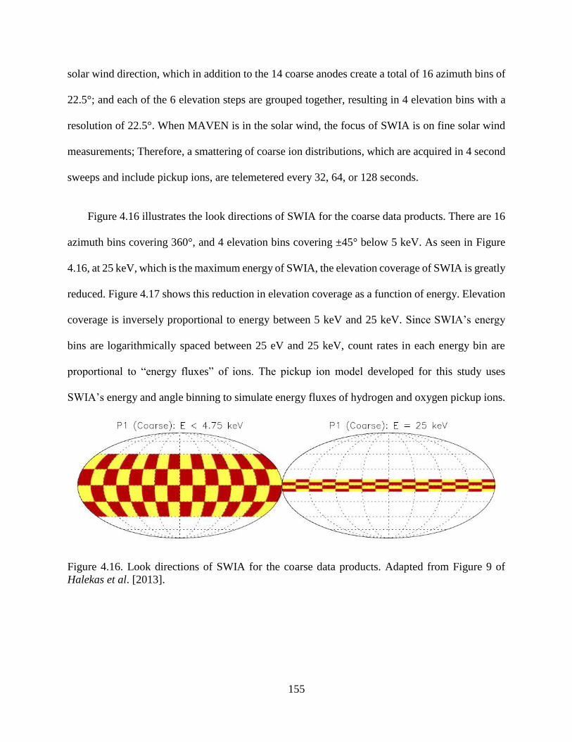
155

solar wind direction, which in addition to the 14 coarse anodes create a total of 16 azimuth bins of

22.5°; and each of the 6 elevation steps are grouped together, resulting in 4 elevation bins with a

resolution of 22.5°. When MAVEN is in the solar wind, the focus of SWIA is on fine solar wind

measurements; Therefore, a smattering of coarse ion distributions, which are acquired in 4 second

sweeps and include pickup ions, are telemetered every 32, 64, or 128 seconds.

Figure 4.16 illustrates the look directions of SWIA for the coarse data products. There are 16

azimuth bins covering 360°, and 4 elevation bins covering ±45° below 5 keV. As seen in Figure

4.16, at 25 keV, which is the maximum energy of SWIA, the elevation coverage of SWIA is greatly

reduced. Figure 4.17 shows this reduction in elevation coverage as a function of energy. Elevation

coverage is inversely proportional to energy between 5 keV and 25 keV. Since SWIA’s energy

bins are logarithmically spaced between 25 eV and 25 keV, count rates in each energy bin are

proportional to “energy fluxes” of ions. The pickup ion model developed for this study uses

SWIA’s energy and angle binning to simulate energy fluxes of hydrogen and oxygen pickup ions.

Figure 4.16. Look directions of SWIA for the coarse data products. Adapted from Figure 9 of

Halekas et al. [2013].

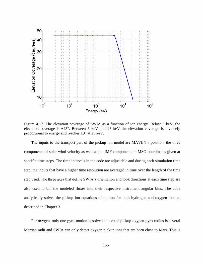
156

Figure 4.17. The elevation coverage of SWIA as a function of ion energy. Below 5 keV, the

elevation coverage is ±45°. Between 5 keV and 25 keV the elevation coverage is inversely

proportional to energy and reaches ±9° at 25 keV.

The inputs to the transport part of the pickup ion model are MAVEN’s position, the three

components of solar wind velocity as well as the IMF components in MSO coordinates given at

specific time steps. The time intervals in the code are adjustable and during each simulation time

step, the inputs that have a higher time resolution are averaged in time over the length of the time

step used. The three axes that define SWIA’s orientation and look directions at each time step are

also used to bin the modeled fluxes into their respective instrument angular bins. The code

analytically solves the pickup ion equations of motion for both hydrogen and oxygen ions as

described in Chapter 3.

For oxygen, only one gyro-motion is solved, since the pickup oxygen gyro-radius is several

Martian radii and SWIA can only detect oxygen pickup ions that are born close to Mars. This is

157

due to the lower geometric factor of SWIA compared to that of the SEP instrument, which limits

SWIA’s ability to measure fluxes from oxygen ions that are created far upstream of Mars where

neutral densities are low. The smaller gyro-radius of hydrogen pickup ions, on the other hand,

entails that the pickup ions code solves at least 5 gyro-motions for pickup hydrogen to ensure all

of the flux from ions created upstream is captured in the simulation. The oxygen exospheric density

profile used in the pickup ion model is adapted from Rahmati et al. [2014] and also described in

Chapter 2, and the hydrogen exospheric density profile is adapted from Feldman et al. [2011].

4.2.1 Orbit 438

Figure 4.18 shows the pickup ion model inputs as well as the one dimensional (1D) SWIA

data, which are summed over all angles and compared to the 1D modeled pickup ion fluxes for a

2-hour time period of orbit 438 starting at 17:30 UTC on 20 December 2014. The panels are as

described in Figure 4.11, with the exception that ionization frequencies now include both oxygen

and hydrogen species and that the last two panels are SWIA data and modeled 1D spectrograms.

It is seen that the solar wind speed fluctuates between 350 km/s and 380 km/s, which means that

the solar wind speed for this time period is too low for pickup oxygen ions to gain enough energy

to be detectable by SEP. As described in Chapter 3, all three components of the solar wind velocity

are used in simulating pickup oxygen and hydrogen ions upstream of Mars.

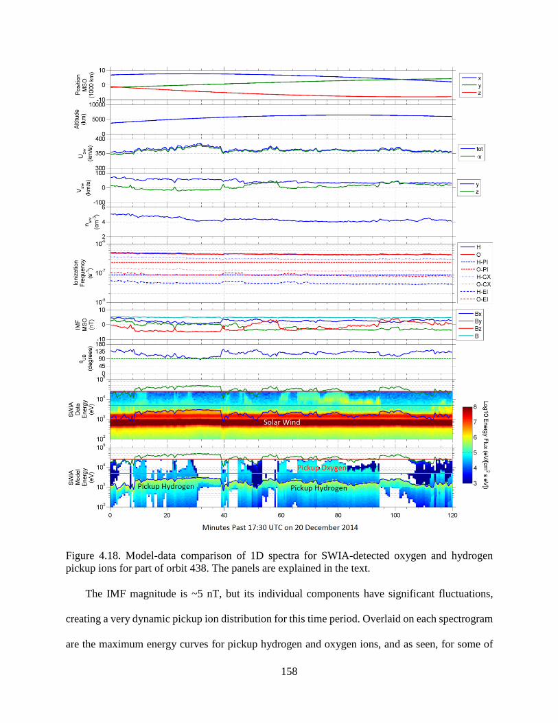
158


pickup ions for part of orbit 438. The panels are explained in the text.

The IMF magnitude is ~5 nT, but its individual components have significant fluctuations,

creating a very dynamic pickup ion distribution for this time period. Overlaid on each spectrogram

are the maximum energy curves for pickup hydrogen and oxygen ions, and as seen, for some of

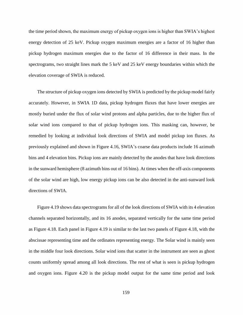
159

the time period shown, the maximum energy of pickup oxygen ions is higher than SWIA’s highest

energy detection of 25 keV. Pickup oxygen maximum energies are a factor of 16 higher than

pickup hydrogen maximum energies due to the factor of 16 difference in their mass. In the

spectrograms, two straight lines mark the 5 keV and 25 keV energy boundaries within which the

elevation coverage of SWIA is reduced.

The structure of pickup oxygen ions detected by SWIA is predicted by the pickup model fairly

accurately. However, in SWIA 1D data, pickup hydrogen fluxes that have lower energies are

mostly buried under the flux of solar wind protons and alpha particles, due to the higher flux of

solar wind ions compared to that of pickup hydrogen ions. This masking can, however, be

remedied by looking at individual look directions of SWIA and model pickup ion fluxes. As

previously explained and shown in Figure 4.16, SWIA’s coarse data products include 16 azimuth

bins and 4 elevation bins. Pickup ions are mainly detected by the anodes that have look directions

in the sunward hemisphere (8 azimuth bins out of 16 bins). At times when the off-axis components

of the solar wind are high, low energy pickup ions can be also detected in the anti-sunward look

directions of SWIA.

Figure 4.19 shows data spectrograms for all of the look directions of SWIA with its 4 elevation

channels separated horizontally, and its 16 anodes, separated vertically for the same time period

as Figure 4.18. Each panel in Figure 4.19 is similar to the last two panels of Figure 4.18, with the

abscissae representing time and the ordinates representing energy. The Solar wind is mainly seen

in the middle four look directions. Solar wind ions that scatter in the instrument are seen as ghost

counts uniformly spread among all look directions. The rest of what is seen is pickup hydrogen

and oxygen ions. Figure 4.20 is the pickup model output for the same time period and look

160

directions as Figure 4.19. A good agreement is seen between the model results and the data. Both

pickup oxygen and pickup hydrogen ions are seen; although at times the maximum energy for

pickup oxygen is higher than SWIA’s high energy threshold of 25 keV. Also, due to the reduction

in the elevation coverage of SWIA, pickup oxygen ions with energies above 5 keV are detected in

a narrower than usual elevation coverage. Therefore, only a small part of pickup oxygen fluxes

that lie within SWIA’s energy and angular coverage are detected by SWIA.

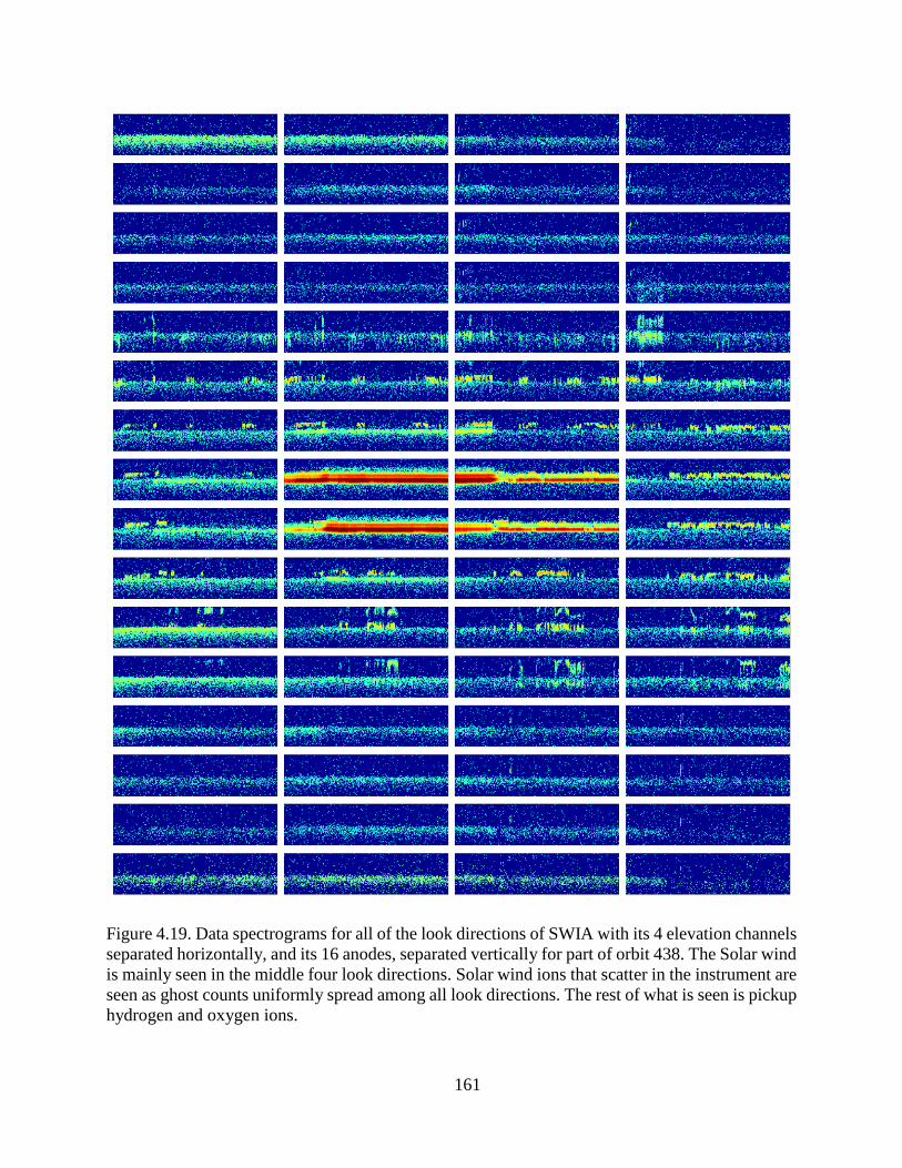
161

Figure 4.19. Data spectrograms for all of the look directions of SWIA with its 4 elevation channels

separated horizontally, and its 16 anodes, separated vertically for part of orbit 438. The Solar wind

is mainly seen in the middle four look directions. Solar wind ions that scatter in the instrument are

seen as ghost counts uniformly spread among all look directions. The rest of what is seen is pickup

hydrogen and oxygen ions.

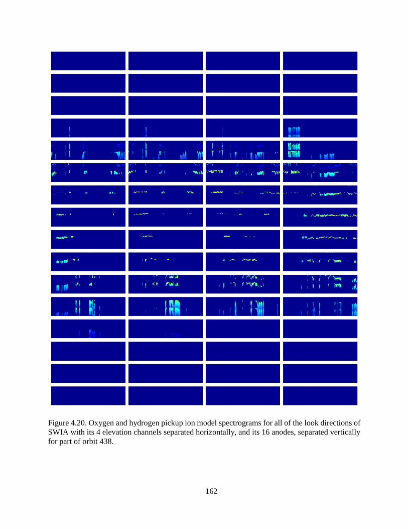
162

Figure 4.20. Oxygen and hydrogen pickup ion model spectrograms for all of the look directions of

SWIA with its 4 elevation channels separated horizontally, and its 16 anodes, separated vertically

for part of orbit 438.

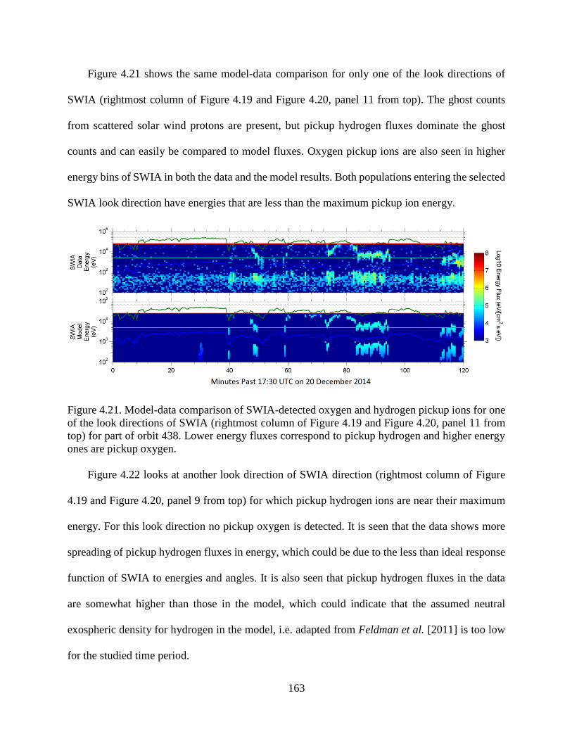
163

Figure 4.21 shows the same model-data comparison for only one of the look directions of

SWIA (rightmost column of Figure 4.19 and Figure 4.20, panel 11 from top). The ghost counts

from scattered solar wind protons are present, but pickup hydrogen fluxes dominate the ghost

counts and can easily be compared to model fluxes. Oxygen pickup ions are also seen in higher

energy bins of SWIA in both the data and the model results. Both populations entering the selected

SWIA look direction have energies that are less than the maximum pickup ion energy.

Figure 4.21. Model-data comparison of SWIA-detected oxygen and hydrogen pickup ions for one

of the look directions of SWIA (rightmost column of Figure 4.19 and Figure 4.20, panel 11 from

top) for part of orbit 438. Lower energy fluxes correspond to pickup hydrogen and higher energy

ones are pickup oxygen.

Figure 4.22 looks at another look direction of SWIA direction (rightmost column of Figure

4.19 and Figure 4.20, panel 9 from top) for which pickup hydrogen ions are near their maximum

energy. For this look direction no pickup oxygen is detected. It is seen that the data shows more

spreading of pickup hydrogen fluxes in energy, which could be due to the less than ideal response

function of SWIA to energies and angles. It is also seen that pickup hydrogen fluxes in the data

are somewhat higher than those in the model, which could indicate that the assumed neutral

exospheric density for hydrogen in the model, i.e. adapted from Feldman et al. [2011] is too low

for the studied time period.

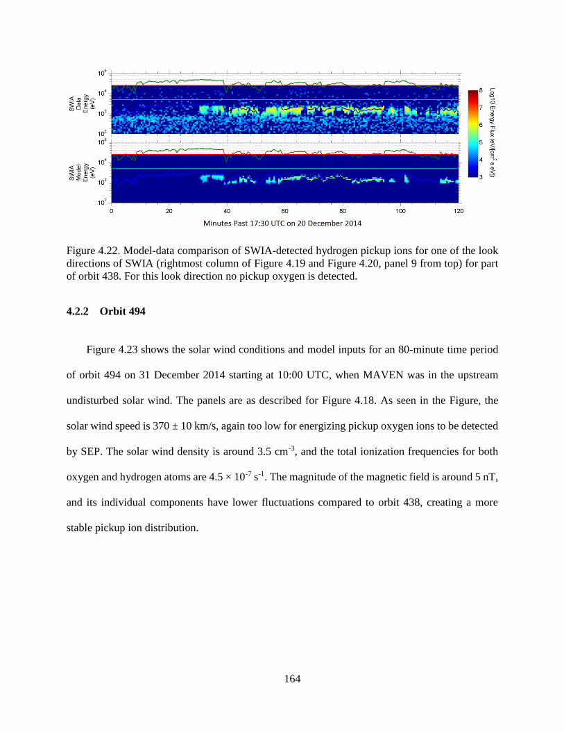
164

Figure 4.22. Model-data comparison of SWIA-detected hydrogen pickup ions for one of the look

directions of SWIA (rightmost column of Figure 4.19 and Figure 4.20, panel 9 from top) for part

of orbit 438. For this look direction no pickup oxygen is detected.

4.2.2 Orbit 494

Figure 4.23 shows the solar wind conditions and model inputs for an 80-minute time period

of orbit 494 on 31 December 2014 starting at 10:00 UTC, when MAVEN was in the upstream

undisturbed solar wind. The panels are as described for Figure 4.18. As seen in the Figure, the

solar wind speed is 370 ± 10 km/s, again too low for energizing pickup oxygen ions to be detected

by SEP. The solar wind density is around 3.5 cm-3, and the total ionization frequencies for both

oxygen and hydrogen atoms are 4.5 × 10-7 s-1. The magnitude of the magnetic field is around 5 nT,

and its individual components have lower fluctuations compared to orbit 438, creating a more

stable pickup ion distribution.

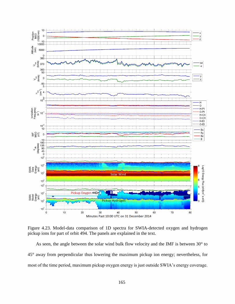
165


pickup ions for part of orbit 494. The panels are explained in the text.

As seen, the angle between the solar wind bulk flow velocity and the IMF is between 30° to

45° away from perpendicular thus lowering the maximum pickup ion energy; nevertheless, for

most of the time period, maximum pickup oxygen energy is just outside SWIA’s energy coverage.

166

High energy pickup oxygen fluxes are seen to increase just after the 30 minute and the 40 minute

marks, due to the change in the Z component of the IMF, as well as a slight increase in the -Z

component of the solar wind velocity. Pickup hydrogen ions are again buried under solar wind

protons and alpha fluxes in the 1D data, and one needs to look at individual look directions of

SWIA to bring out the angular distribution.

Figure 4.24 and Figure 4.25 represent the SWIA measured and the simulated pickup ion

fluxes, respectively, for different SWIA look directions and for the same time period shown in

Figure 4.23. Again, a good agreement is seen between the model output and the data. Figure 4.26

shows the model-data comparison for only one of the look directions of SWIA (rightmost column

of Figure 4.24 and Figure 4.25, panel 11 from top) for the same time period. It appears that the

pickup hydrogen fluxes in the data are more spread out in energy and have higher values compared

to the model. Also, during the first 30 minutes of data, some pickup hydrogen is detected by SWIA

that is not predicted by the model. This could again be due to the non-perfect angular resolution

of SWIA and that the pickup ions seen are leaking from the neighboring look directions.

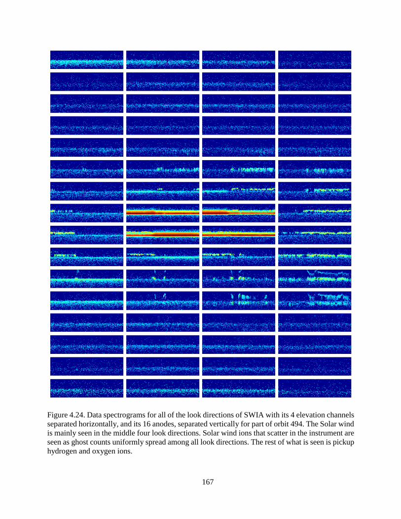
167

Figure 4.24. Data spectrograms for all of the look directions of SWIA with its 4 elevation channels

separated horizontally, and its 16 anodes, separated vertically for part of orbit 494. The Solar wind

is mainly seen in the middle four look directions. Solar wind ions that scatter in the instrument are

seen as ghost counts uniformly spread among all look directions. The rest of what is seen is pickup

hydrogen and oxygen ions.

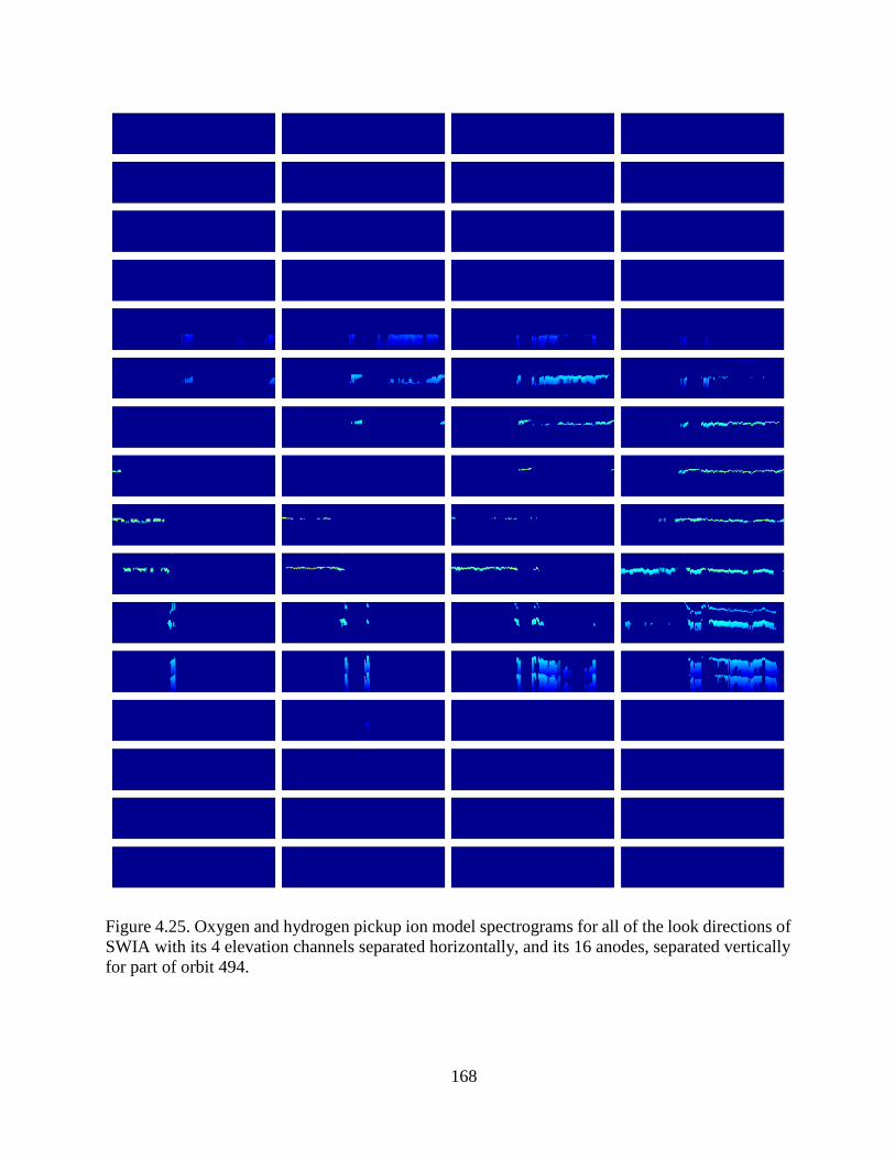
168

Figure 4.25. Oxygen and hydrogen pickup ion model spectrograms for all of the look directions of

SWIA with its 4 elevation channels separated horizontally, and its 16 anodes, separated vertically

for part of orbit 494.

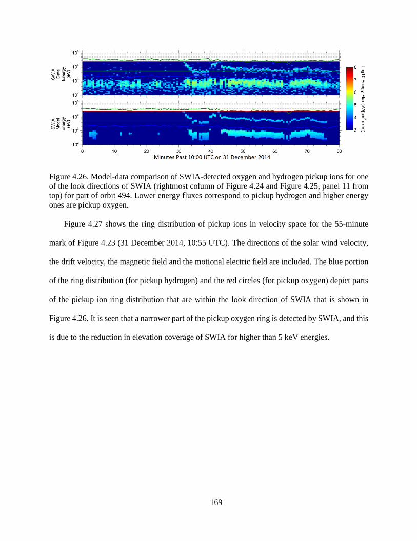
169


of the look directions of SWIA (rightmost column of Figure 4.24 and Figure 4.25, panel 11 from

top) for part of orbit 494. Lower energy fluxes correspond to pickup hydrogen and higher energy

ones are pickup oxygen.

Figure 4.27 shows the ring distribution of pickup ions in velocity space for the 55-minute

mark of Figure 4.23 (31 December 2014, 10:55 UTC). The directions of the solar wind velocity,

the drift velocity, the magnetic field and the motional electric field are included. The blue portion

of the ring distribution (for pickup hydrogen) and the red circles (for pickup oxygen) depict parts

of the pickup ion ring distribution that are within the look direction of SWIA that is shown in

Figure 4.26. It is seen that a narrower part of the pickup oxygen ring is detected by SWIA, and this

is due to the reduction in elevation coverage of SWIA for higher than 5 keV energies.

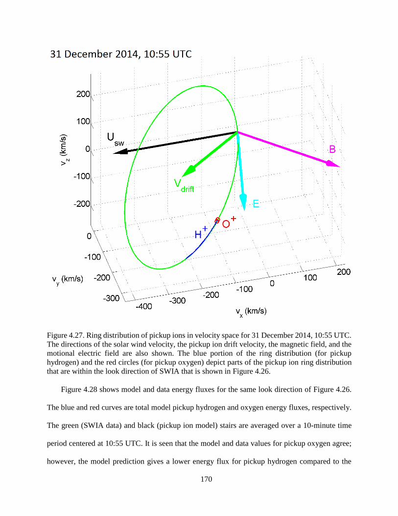
170

Figure 4.27. Ring distribution of pickup ions in velocity space for 31 December 2014, 10:55 UTC.

The directions of the solar wind velocity, the pickup ion drift velocity, the magnetic field, and the

motional electric field are also shown. The blue portion of the ring distribution (for pickup

hydrogen) and the red circles (for pickup oxygen) depict parts of the pickup ion ring distribution

that are within the look direction of SWIA that is shown in Figure 4.26.

Figure 4.28 shows model and data energy fluxes for the same look direction of Figure 4.26.

The blue and red curves are total model pickup hydrogen and oxygen energy fluxes, respectively.

The green (SWIA data) and black (pickup ion model) stairs are averaged over a 10-minute time

period centered at 10:55 UTC. It is seen that the model and data values for pickup oxygen agree;

however, the model prediction gives a lower energy flux for pickup hydrogen compared to the

171

SWIA data by a factor of ~3. The agreement between the SWIA data and the modeled oxygen

pickup ion fluxes for this case indicates that the two-stream/Liouville model described in Chapter

2 and used to calculate the hot oxygen escape fluxes appears to be correct. The disagreement

between the SWIA data and the modeled hydrogen pickup ion fluxes means that for this time

period we need an exospheric hydrogen density that is a factor of ~3 higher than the Feldman et

al. [2011] profile.

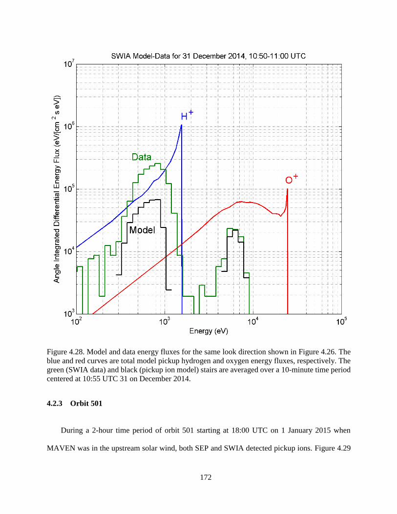
172

Figure 4.28. Model and data energy fluxes for the same look direction shown in Figure 4.26. The

blue and red curves are total model pickup hydrogen and oxygen energy fluxes, respectively. The

green (SWIA data) and black (pickup ion model) stairs are averaged over a 10-minute time period

centered at 10:55 UTC 31 on December 2014.

4.2.3 Orbit 501

During a 2-hour time period of orbit 501 starting at 18:00 UTC on 1 January 2015 when

MAVEN was in the upstream solar wind, both SEP and SWIA detected pickup ions. Figure 4.29

173

shows the solar wind input parameters for this time period in the top panels and as seen the IMF

components have fairly high fluctuations. The solar wind speed is above 500 km/s and SEP is able

to detect oxygen pickup ions. The SEP data and model results are shown for SEP1F and SEP2F in

the middle panels, and as seen the pickup model accurately predicts the pickup oxygen features

measured by SEP. As seen in the SWIA model and data panels at the bottom, SWIA is mainly

detecting pickup hydrogen during this time period, and only for a few minutes, pickup oxygen is

within the FOV of SWIA.

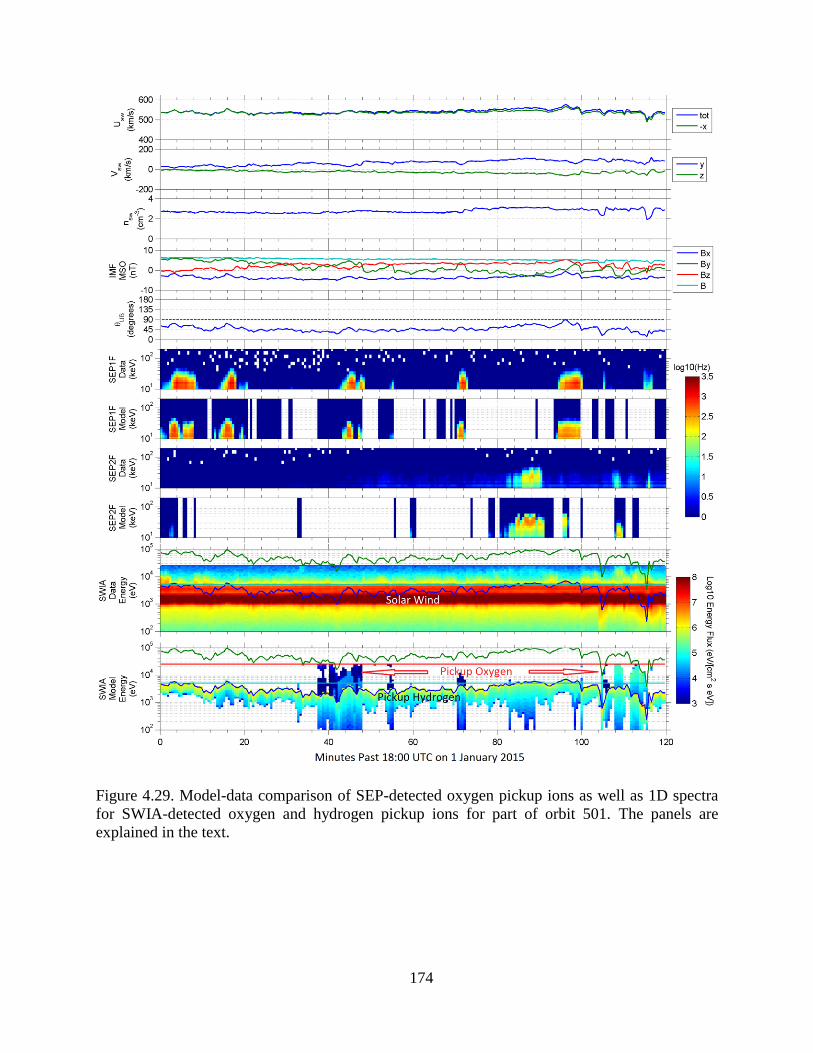
174

Figure 4.29. Model-data comparison of SEP-detected oxygen pickup ions as well as 1D spectra

for SWIA-detected oxygen and hydrogen pickup ions for part of orbit 501. The panels are

explained in the text.

175

4.2.4 Orbit 336

The early hours of December 2014 were another period when both the SEP and the SWIA

instruments detected pickup ions. Figure 4.30 shows a 110-minute time period of orbit 336 starting

at 05:40 UTC on 1 December 2014, with the solar wind conditions plotted in the first 5 panels,

and the SEP2F and SWIA data and model results plotted in the last 4 panels. As seen, the solar

wind speed is above 450 km/s for the whole time period and SEP was able to detect oxygen pickup

ions. SEP2F had a close to sunward look direction and its attenuator was closed to protect the

silicon detector from sunlight. Therefore, the data count rates shown are multiplied by a factor of

100. The SWIA data and model results are for only one anode of SWIA and integrated over all

elevations for that anode. The selected anode does not have the solar wind in its FOV, and the

background counts are due to the scattered solar wind ions in the instrument.

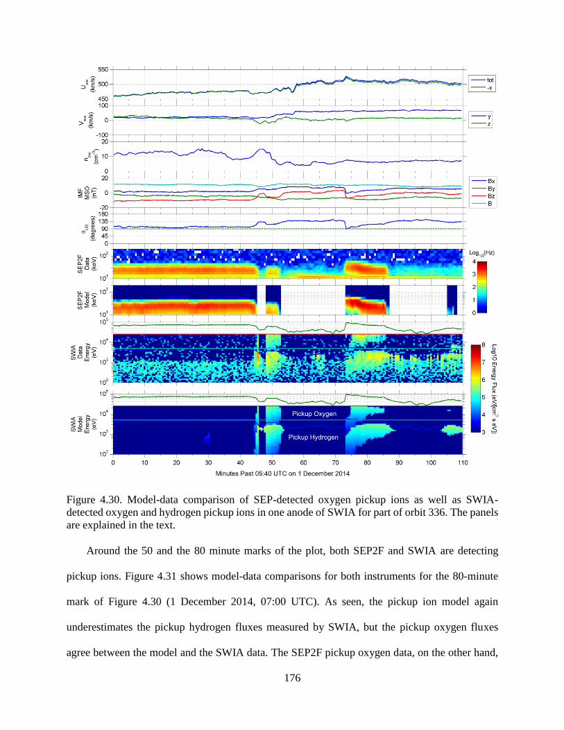
176

Figure 4.30. Model-data comparison of SEP-detected oxygen pickup ions as well as SWIA-

detected oxygen and hydrogen pickup ions in one anode of SWIA for part of orbit 336. The panels

are explained in the text.

Around the 50 and the 80 minute marks of the plot, both SEP2F and SWIA are detecting

pickup ions. Figure 4.31 shows model-data comparisons for both instruments for the 80-minute

mark of Figure 4.30 (1 December 2014, 07:00 UTC). As seen, the pickup ion model again

underestimates the pickup hydrogen fluxes measured by SWIA, but the pickup oxygen fluxes

agree between the model and the SWIA data. The SEP2F pickup oxygen data, on the other hand,

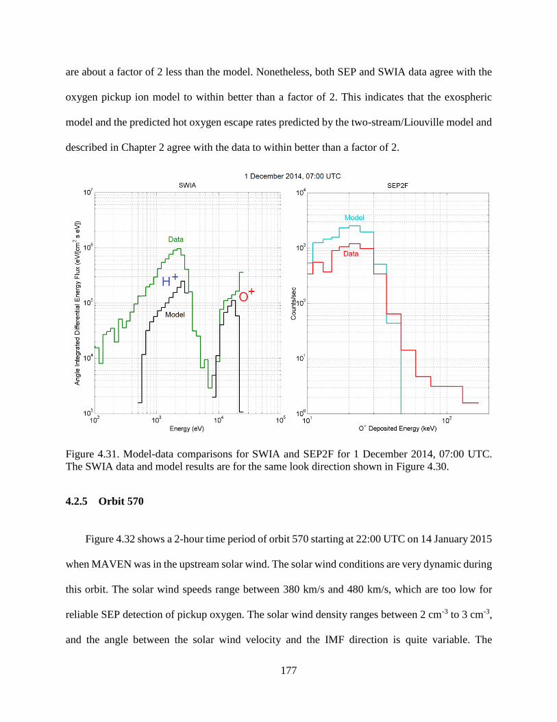
177

are about a factor of 2 less than the model. Nonetheless, both SEP and SWIA data agree with the

oxygen pickup ion model to within better than a factor of 2. This indicates that the exospheric

model and the predicted hot oxygen escape rates predicted by the two-stream/Liouville model and

described in Chapter 2 agree with the data to within better than a factor of 2.

Figure 4.31. Model-data comparisons for SWIA and SEP2F for 1 December 2014, 07:00 UTC.

The SWIA data and model results are for the same look direction shown in Figure 4.30.

4.2.5 Orbit 570

Figure 4.32 shows a 2-hour time period of orbit 570 starting at 22:00 UTC on 14 January 2015

when MAVEN was in the upstream solar wind. The solar wind conditions are very dynamic during

this orbit. The solar wind speeds range between 380 km/s and 480 km/s, which are too low for

reliable SEP detection of pickup oxygen. The solar wind density ranges between 2 cm-3 to 3 cm-3,

and the angle between the solar wind velocity and the IMF direction is quite variable. The

178

spectrograms in the last two panels, show the SWIA data and model results for one of SWIA’s

anodes (one azimuth), integrated over all elevations. The selected anode had most of the pickup

oxygen distribution within its FOV, and although the solar wind was outside the FOV of the anode,

ghost counts from scattered solar wind protons are present in the data spectra, contaminating the

pickup hydrogen counts.

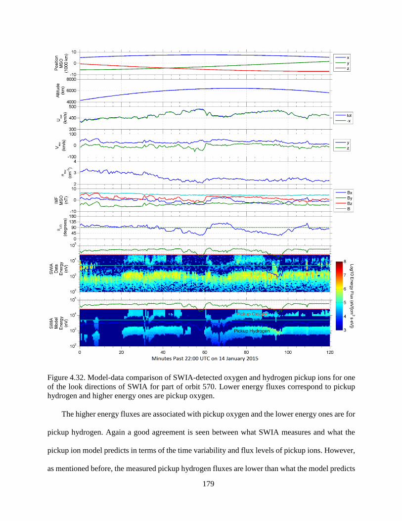
179


of the look directions of SWIA for part of orbit 570. Lower energy fluxes correspond to pickup

hydrogen and higher energy ones are pickup oxygen.

The higher energy fluxes are associated with pickup oxygen and the lower energy ones are for

pickup hydrogen. Again a good agreement is seen between what SWIA measures and what the

pickup ion model predicts in terms of the time variability and flux levels of pickup ions. However,

as mentioned before, the measured pickup hydrogen fluxes are lower than what the model predicts

180

and this can be caused by the too low hydrogen exospheric densities assumed for this time period.

The agreement in flux levels for pickup oxygen in the above model-data comparisons gives us

confidence in the oxygen exospheric density profile used in the pickup model.

181

5 Conclusions

In this work the processes that populate the extended hot oxygen exosphere at Mars were

described and oxygen pickup ion model-data comparisons were provided to confirm the existence

of the Martian oxygen exosphere. The main process that creates hot oxygen atoms is the

dissociative recombination (DR) of ionospheric O2+ ions with electrons in the Martian ionosphere.

Some of the produced hot oxygen atoms have speeds exceeding the escape speed and thus

contribute to atmospheric loss. It was shown in Chapter 2 that the escaping portion of the neutral

oxygen exosphere at Mars is small and only dominant at distances greater than 10-15 Martian

radii. Hence, a means of detecting distant or escaping neutral oxygen is needed in order to constrain

the hot oxygen exosphere and obtain an observational check on hot O escape calculations.

A major goal of the MAVEN mission to Mars is to quantify atmospheric loss processes, and

an important loss process is the photochemical escape of neutral oxygen via the DR reaction.

However, the photochemical escape rate calculations vary by about two orders of magnitude and

there is a lack of direct observational constraint on photochemical escape models. This uncertainty

in calculated escape rates results in different estimates of out-gassed water from Mars. The two-

stream/Liouville model presented in Chapter 2 and cross-checked with a Monte-Carlo transport

model estimates that for moderate solar wind conditions 5 × 1025 hot oxygen atoms leave Mars

every second via the photo-chemical escape process. This amounts to the removal of a 1-meter

layer of water from Mars over the 4.5 billion years of Mars history, assuming that the escape rate

remained constant over time.

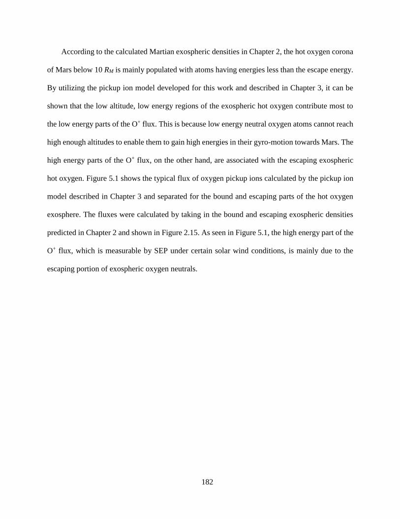
182

According to the calculated Martian exospheric densities in Chapter 2, the hot oxygen corona

of Mars below 10 RM is mainly populated with atoms having energies less than the escape energy.

By utilizing the pickup ion model developed for this work and described in Chapter 3, it can be

shown that the low altitude, low energy regions of the exospheric hot oxygen contribute most to

the low energy parts of the O+ flux. This is because low energy neutral oxygen atoms cannot reach

high enough altitudes to enable them to gain high energies in their gyro-motion towards Mars. The

high energy parts of the O+ flux, on the other hand, are associated with the escaping exospheric

hot oxygen. Figure 5.1 shows the typical flux of oxygen pickup ions calculated by the pickup ion

model described in Chapter 3 and separated for the bound and escaping parts of the hot oxygen

exosphere. The fluxes were calculated by taking in the bound and escaping exospheric densities

predicted in Chapter 2 and shown in Figure 2.15. As seen in Figure 5.1, the high energy part of the

O+ flux, which is measurable by SEP under certain solar wind conditions, is mainly due to the

escaping portion of exospheric oxygen neutrals.

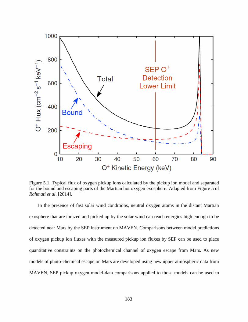
183

Figure 5.1. Typical flux of oxygen pickup ions calculated by the pickup ion model and separated

for the bound and escaping parts of the Martian hot oxygen exosphere. Adapted from Figure 5 of


In the presence of fast solar wind conditions, neutral oxygen atoms in the distant Martian

exosphere that are ionized and picked up by the solar wind can reach energies high enough to be

detected near Mars by the SEP instrument on MAVEN. Comparisons between model predictions

of oxygen pickup ion fluxes with the measured pickup ion fluxes by SEP can be used to place

quantitative constraints on the photochemical channel of oxygen escape from Mars. As new

models of photo-chemical escape on Mars are developed using new upper atmospheric data from

MAVEN, SEP pickup oxygen model-data comparisons applied to those models can be used to

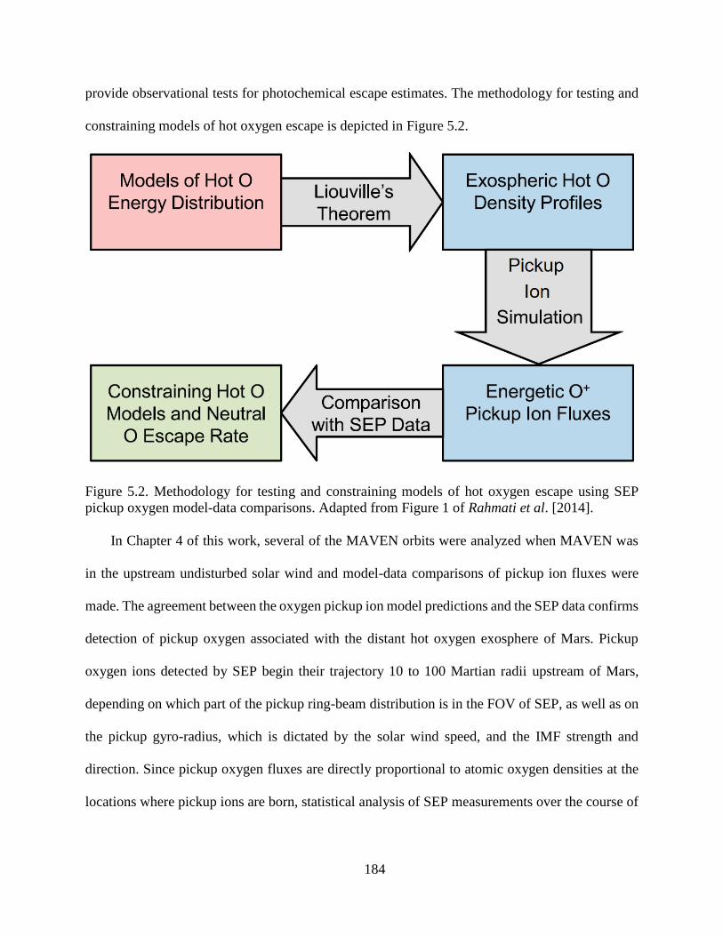
184

provide observational tests for photochemical escape estimates. The methodology for testing and

constraining models of hot oxygen escape is depicted in Figure 5.2.

Figure 5.2. Methodology for testing and constraining models of hot oxygen escape using SEP

pickup oxygen model-data comparisons. Adapted from Figure 1 of Rahmati et al. [2014].

In Chapter 4 of this work, several of the MAVEN orbits were analyzed when MAVEN was

in the upstream undisturbed solar wind and model-data comparisons of pickup ion fluxes were

made. The agreement between the oxygen pickup ion model predictions and the SEP data confirms

detection of pickup oxygen associated with the distant hot oxygen exosphere of Mars. Pickup

oxygen ions detected by SEP begin their trajectory 10 to 100 Martian radii upstream of Mars,

depending on which part of the pickup ring-beam distribution is in the FOV of SEP, as well as on

the pickup gyro-radius, which is dictated by the solar wind speed, and the IMF strength and

direction. Since pickup oxygen fluxes are directly proportional to atomic oxygen densities at the

locations where pickup ions are born, statistical analysis of SEP measurements over the course of

185

the entire MAVEN mission will enable the exospheric neutral oxygen densities to be constrained

at different locations upstream of Mars.

It was shown in Chapter 4 that the SWIA instrument is also able to detect hydrogen and

oxygen pickup ions outside the Martian bow shock. Since SWIA has a geometric factor that is

much lower than that of the SEP instrument, and because SWIA cannot detect pickup ions with

energies above 25 keV, the SWIA measured pickup ions are associated with the low altitude parts

of the Martian exosphere, where densities are higher and the neutral oxygen is mainly bound.

Therefore, comparing the SWIA measured pickup ions with the model predicted ones can assist

the MAVEN IUVS instrument in constraining the low altitude parts of the Martian oxygen corona.

Oxygen pickup ion model-data comparisons provided in Chapter 4 indicate that the model hot

oxygen flux calculations discussed in Chapter 2 agree with the SWIA and SEP data to within better

than a factor of 2 to 3. This means that the two-stream and the Monte-Carlo models used in this

work predict hot oxygen escape rates that are accurate to within better than a factor of 2 to 3. This

would place the photo-chemical escape rate of neutral oxygen atoms predicted by this work (5 ×

1025 s-1) about one order of magnitude higher than the average value for the modeled and measured

escape rate of oxygen ions (a few times 1024 s-1).

For future work, this pickup ion technique can be used to assess other hot oxygen models that

are present within the scientific community and will be developed based on the new MAVEN

results. This work did not include the CO2+ DR as the source of production of hot O. Recent models

predict that the CO2+ DR can be an important source of hot O escape under certain conditions

[Gröller et al., 2014] and future work can address this. The 3D Monte-Carlo transport method

described in Section 2.2.5 used ionospheric inputs from the MTGCM for a single location on Mars.

186

The code can be used in the future to include location-dependent inputs and hot O production rates.

Therefore, a more realistic modeling of the Martian hot O exosphere by the 3D Monte-Carlo code

is possible and future work can determine how the non-spherically symmetric production of hot

oxygen atoms would affect the distribution of hot O atoms in the exosphere on Mars.

In summary, the following has been accomplished in this work:

The production of hot oxygen atoms in the upper atmosphere of Mars was calculated using

the molecular oxygen ion and electron densities and temperatures.

A Monte-Carlo code was developed to calculate the forward and backscattering

probabilities and energy losses for collisions of hot oxygen atoms with atmospheric neutral

species.

A two-stream transport code was used to model the fluxes of hot oxygen atoms for solar

cycle maximum and minimum conditions.

Hot oxygen escape fluxes and rates on Mars were calculated from the outputs of the two-

stream code.

A Liouville code was used to extend the hot oxygen distribution to high altitudes in the

Martian exosphere and to find the escaping and bound portions of hot oxygen exospheric

densities.

A 3D Monte-Carlo transport code was developed to cross-check the results of the two-

stream/Liouville codes.

A code was developed to access and analyze the MAVEN data from the SEP, SWIA,

SWEA, MAG, and EUVM instruments.

Ionization rates of oxygen and hydrogen atoms in the solar wind were calculated based on

contributions from photo-ionization using the EUVM data, charge exchange using the

SWIA data, and electron impact ionization using the SWEA data.

A pickup ion trajectory solver code was developed to track the gyro-motion of oxygen and

hydrogen pickup ions in the upstream, undisturbed, and uniform solar wind fields using

the MAG and SWIA data.

Fluxes of oxygen and hydrogen pickup ions were modeled at the location of MAVEN

outside the Martian bow shock and in the upstream undisturbed solar wind.

The SEP and SWIA instrumental geometry, look direction, field of view, and response

function to energy and angular distribution of pickup ions were used to model the pickup

ion measurements by SEP and SWIA.

187

Oxygen pickup ion flux model-data comparisons were provided for several of the MAVEN

orbits, showing the agreement between the model predictions and the data to within better

than a factor of 2 to 3.

A methodology was described that can constrain models of the Mars hot oxygen

distribution and escape by comparing the SEP and SWIA data with pickup ion model

predictions.

Model-data comparisons indicate that the predicted exospheric oxygen densities and the

photo-chemical escape rate of 5 × 1025 hot oxygen atoms per second by the two-

stream/Liouville and the Monte-Carlo models agree with the SEP and SWIA data to within

better than a factor of 2 to 3.

188

References

Acuna, M. H., et al. (1999), Global distribution of crustal magnetization discovered by the Mars

Global Surveyor MAG/ER experiment, Science, 284(5415), 790-793,

doi:10.1126/science.284.5415.790.

Agostinelli, S., et al. (2003), GEANT4—a simulation toolkit, Nucl. Instrum. Methods, 506(3), 250-

303, doi:10.1016/S0168-9002(03)01368-8.

Allison, J., et al. (2006), Geant4 developments and applications, IEEE Trans. Nucl. Sci., 53(1),

270-278, doi:10.1109/TNS.2006.869826.

Anderson, D. E., and C. W. Hord (1971), Mariner 6 and 7 Ultraviolet Spectrometer Experiment:

Analysis of hydrogen Lyman-alpha data, J. Geophys. Res., 76(28), 6666–6673,

doi:10.1029/JA076i028p06666.

Anderson, D. E. (1974), Mariner 6, 7, and 9 Ultraviolet Spectrometer Experiment: Analysis of

hydrogen Lyman alpha data, J. Geophys. Res., 79(10), 1513–1518,

doi:10.1029/JA079i010p01513.

Andersson, L., et al. (2015a), The Langmuir probe and waves (LPW) instrument for MAVEN,

Space Sci. Rev., doi:10.1007/s11214-015-0194-3.

Andersson, L., et al. (2015b), Dust observations at orbital altitudes surrounding Mars, Science,

doi:10.1126/science.aad0398.

Andrews, D. J., L. Andersson, G. T. Delory, R. E. Ergun, A. I. Eriksson, C. M. Fowler, T.

McEnulty, M. W. Morooka, T. Weber, and B. M. Jakosky (2015), Ionospheric plasma density

variations observed at Mars by MAVEN/LPW, Geophys. Res. Lett., 42, 8862–8869,

doi:10.1002/2015GL065241.

Angel, G. C., and J. A. Samson (1988), Total photoionization cross sections of atomic oxygen

from threshold to 44.3 Å, Phys. Rev. A, 38(11), 5578, doi:10.1103/PhysRevA.38.5578.

Balakrishnan, N., V. Kharchenko, and A. Dalgarno (1998), Slowing of energetic O(3P) atoms in

collisions with N2, J. Geophys. Res., 103(A10), 23393–23398, doi:10.1029/98JA02198.

Barabash, S., E. Dubinin, N. Pissarenko, R. Lundin, and C. T. Russell (1991), Picked-up protons

near Mars: Phobos observations, Geophys. Res. Lett., 18(10), 1805-1808,

doi:10.1029/91GL02082.

Barabash, S., A. Fedorov, R. Lundin, and J. A. Sauvaud (2007), Martian Atmospheric Erosion

Rates, Science, 315(5811), 501-503, doi:10.1126/science.1134358.

https://dx.doi.org/10.1126/science.284.5415.790

https://dx.doi.org/10.1016/S0168-9002(03)01368-8

https://dx.doi.org/10.1109/TNS.2006.869826

https://dx.doi.org/10.1029/JA076i028p06666

https://doi.org10.1029/JA079i010p01513

https://dx.doi.org/10.1007/s11214-015-0194-3

https://dx.doi.org/10.1126/science.aad0398

https://dx.doi.org/10.1002/2015GL065241

https://dx.doi.org/10.1103/PhysRevA.38.5578

https://dx.doi.org/10.1029/98JA02198


https://dx.doi.org/10.1126/science.1134358

189

Benna, M., P. R. Mahaffy, J. M. Grebowsky, J. L. Fox, R. V. Yelle, and B. M. Jakosky (2015),

First measurements of composition and dynamics of the Martian ionosphere by MAVEN’s

Neutral Gas and Ion Mass Spectrometer, Geophys. Res. Lett., 42,

doi:10.1002/2015GL066146.

Bhattacharyya, D., J. T. Clarke, J.-L. Bertaux, J.-Y. Chaufray, and M. Mayyasi (2015), A strong

seasonal dependence in the Martian hydrogen exosphere, Geophys. Res. Lett., 42, 8678–8685,

doi:10.1002/2015GL065804.

Bougher, S. W., A. Valeille, M. R. Combi, and V. Tenishev (2009), Solar cycle and seasonal

variability of the Martian thermosphere-ionosphere and associated impacts upon atmospheric

escape, SAE Technical Paper 2009-01-2386, SAE International.

Bougher, S. W. (2012), Coupled MGCM-MTGCM Mars Thermosphere Simulations and

Resulting Data Products in Support of the MAVEN Mission, JPL/CDP report, pp. 1-9, 6-

August-2012.

Bougher, S. W., T. E. Cravens, J. Grebowsky, and J. Luhmann (2014), The aeronomy of Mars:

Characterization by MAVEN of the upper atmosphere reservoir that regulates volatile escape,

Space Sci. Rev., doi:10.1007/s11214-014-0053-7.

Bougher, S. W., et al. (2015), Early MAVEN Deep Dip campaign reveals thermosphere and

ionosphere variability, Science, 350(6261), doi:10.1126/science.aad0459.

Brain, D. A., and B. M. Jakosky (1998), Atmospheric loss since the onset of the Martian geologic

record: Combined role of impact erosion and sputtering, J. Geophys. Res., 103(E10), 22689-

22694, doi:10.1029/98JE02074.

Brain, D. A., et al. (2015), The spatial distribution of planetary ion fluxes near Mars observed by

MAVEN, Geophys. Res. Lett., 42, 9142–9148, doi:10.1002/2015GL065293.

Carr, M. H. (1987), Water on Mars, Nature, 326(6108), 30-35, doi:10.1038/326030a0.

Carr, M. H. (1996), Water on Mars, Oxford University Press, New York.

Chaffin, M. S., et al. (2015), Three-dimensional structure in the Mars H corona revealed by IUVS

on MAVEN, Geophys. Res. Lett., 42, 9001–9008, doi:10.1002/2015GL065287.

Chamberlin, P. C., T. N. Woods, and F. G. Chamberlin (2007), Flare Irradiance Spectral Model

(FISM): Daily component algorithms and results, Space Weather, 5, S07005,

doi:10.1029/2007SW000316.

Chassefière, E., and F. Leblanc (2004), Mars atmospheric escape and evolution: Interaction with

the solar wind, Planet. Space Sci., 52(11), 1039-1058, doi:10.1016/j.pss.2004.07.002.



https://dx.doi.org/10.1007/s11214-014-0053-7


https://dx.doi.org/10.1029/98JE02074


https://dx.doi.org/10.1038/326030a0


https://dx.doi.org/10.1029/2007SW000316

https://dx.doi.org/10.1016/j.pss.2004.07.002

190

Chaufray, J. Y., J. L. Bertaux, F. Leblanc, and E. Quémerais (2008), Observation of the hydrogen

corona with SPICAM on Mars Express, Icarus, 195(2), 598-613,

doi:10.1016/j.icarus.2008.01.009.

Chaufray, J. Y., F. Gonzalez-Galindo, F. Forget, M. Lopez-Valverde, F. Leblanc, R. Modolo, S.

Hess, M. Yagi, P.-L. Blelly, and O. Witasse (2014), Three-dimensional Martian ionosphere

model: II. Effect of transport processes due to pressure gradients, J. Geophys. Res. Planets,

119, 1614–1636, doi:10.1002/2013JE004551.

Chaufray, J. Y., F. Gonzalez-Galindo, F. Forget, M. Lopez-Valverde, F. Leblanc, R. Modolo, and

S. Hess (2015a), Variability of the hydrogen in the martian upper atmosphere as simulated by

a 3D atmosphere–exosphere coupling, Icarus, 245, 282-294,

doi:10.1016/j.icarus.2014.08.038.

Chaufray, J. Y., et al. (2015b), Study of the Martian cold oxygen corona from the O I 130.4 nm by

IUVS/MAVEN, Geophys. Res. Lett., 42, 9031–9039, doi:10.1002/2015GL065341.

Chen, R. H., T. E. Cravens, and A. F. Nagy (1978), The Martian ionosphere in light of the Viking

observations, J. Geophys. Res., 83(A8), 3871–3876, doi:10.1029/JA083iA08p03871.

Clarke, J. T., J.-L. Bertaux, J.-Y. Chaufray, G. R. Gladstone, E. Quemerais, J. K. Wilson, and D.

Bhattacharyya (2014), A rapid decrease of the hydrogen corona of Mars, Geophys. Res. Lett.,

41, 8013–8020, doi:10.1002/2014GL061803.

Coates, A. J. (2004), Ion pickup at comets, Adv. Space Res., 33(11), 1977-1988,

doi:10.1016/j.asr.2003.06.029.

Connerney J. E. P., J. Espley, P. Lawton, S. Murphy, J. Odom, R. Oliversen, and D. Sheppard

(2015a), The MAVEN Magnetic Field Investigation, Space Sci. Rev., doi:10.1007/s11214-

015-0169-4.

Connerney, J. E. P., J. R. Espley, G. A. DiBraccio, J. R. Gruesbeck, R. J. Oliversen, D. L. Mitchell,

J. Halekas, C. Mazelle, D. Brain, and B. M. Jakosky (2015b), First results of the MAVEN

magnetic field investigation, Geophys. Res. Lett., 42, 8819–8827,

doi:10.1002/2015GL065366.

Cravens, T. E., J. U. Kozyra, A. F. Nagy, T. I. Gombosi, and M. Kurtz (1987), Electron impact

ionization in the vicinity of comets, J. Geophys. Res., 92(A7), 7341-7353,

doi:10.1029/JA092iA07p07341.

Cravens, T. E. (1989), Test particle calculations of pick-up ions in the vicinity of comet Giacobini-

Zinner, Planet. Space Sci., 37(10), 1169-1184, doi:10.1016/0032-0633(89)90012-3.

Cravens, T. E., A. Hoppe, S. A. Ledvina, and S. McKenna-Lawlor (2002), Pickup ions near Mars

associated with escaping oxygen atoms, J. Geophys. Res., 107(A8),

doi:10.1029/2001JA000125.

http://dx.doi.org/10.1016/j.icarus.2008.01.009

http://dx.doi.org/10.1002/2013JE004551

https://dx.doi.org/10.1016/j.icarus.2014.08.038


https://dx.doi.org/10.1029/JA083iA08p03871


https://dx.doi.org/10.1016/j.asr.2003.06.029

https://dx.doi.org/10.1007/s11214-015-0169-4

https://dx.doi.org/10.1007/s11214-015-0169-4



https://dx.doi.org/10.1016/0032-0633(89)90012-3


191

Curry, S. M., M. Liemohn, X. Fang, D. Brain, and Y. Ma (2013), Simulated kinetic effects of the

corona and solar cycle on high altitude ion transport at Mars, J. Geophys. Res., 118, 3700–

3711, doi:10.1002/jgra.50358.

Curry, S. M., et al. (2014), Test particle comparison of heavy atomic and molecular ion

distributions at Mars, J. Geophys. Res., 119(3), 2328-2344, doi:10.1002/2013JA019221.

Curry, S. M., et al. (2015), Response of Mars O+ pickup ions to the 8 March 2015 ICME:

Inferences from MAVEN data-based models, Geophys. Res. Lett., 42, 9095–9102,

doi:10.1002/2015GL065304.

Deighan, J., et al. (2015), MAVEN IUVS observation of the hot oxygen corona at Mars, Geophys.

Res. Lett., 42, 9009–9014, doi:10.1002/2015GL065487.

DiBraccio, G. A., et al. (2015), Magnetotail dynamics at Mars: Initial MAVEN observations,

Geophys. Res. Lett., 42, 8828–8837, doi:10.1002/2015GL065248.

Dong, C., S. W. Bougher, Y. Ma, G. Toth, Y. Lee, A. F. Nagy, V. Tenishev, D. J. Pawlowski, M.

R. Combi, and D. Najib (2015a), Solar wind interaction with the Martian upper atmosphere:

Crustal field orientation, solar cycle and seasonal variations, J. Geophys. Res. Space Physics,

doi:10.1002/2015JA020990.

Dong, C., et al. (2015b), Multifluid MHD study of the solar wind interaction with Mars' upper

atmosphere during the 2015 March 8th ICME event, Geophys. Res. Lett., 42, 9103–9112,

doi:10.1002/2015GL065944.

Dong, Y., X. Fang, D. A. Brain, J. P. McFadden, J. S. Halekas, J. E. Connerney, S. M. Curry, Y.

Harada, J. G. Luhmann, and B. M. Jakosky (2015), Strong plume fluxes at Mars observed by

MAVEN: An important planetary ion escape channel, Geophys. Res. Lett., 42, 8942–8950,

doi:10.1002/2015GL065346.

Dubinin, E., M. Fraenz, J. Woch, S. Barabash, R. Lundin, and M. Yamauchi (2006), Hydrogen

exosphere at Mars: Pickup protons and their acceleration at the bow shock, Geophys. Res.

Lett., 33, L22103, doi:10.1029/2006GL027799.

Eparvier, F. G., P. C. Chamberlin, T. N. Woods, and E. M. B. Thiemann (2015), The solar extreme

ultraviolet monitor for MAVEN, Space Sci. Rev., doi:10.1007/s11214-015-0195-2.

Ergun, R. E., M. W. Morooka, L. A. Andersson, C. M. Fowler, G. T. Delory, D. J. Andrews, A. I.

Eriksson, T. McEnulty, and B. M. Jakosky (2015), Dayside electron temperature and density

profiles at Mars: First results from the MAVEN Langmuir probe and waves instrument,


Evans, J. S., et al. (2015), Retrieval of CO2 and N2 in the Martian thermosphere using dayglow

observations by IUVS on MAVEN, Geophys. Res. Lett., 42, 9040–9049,

doi:10.1002/2015GL065489.

https://dx.doi.org/10.1002/jgra.50358





http://dx.doi.org/10.1002/2015JA020990



http://dx.doi.org/10.1029/2006GL027799

https://dx.doi.org/10.1007/s11214-015-0195-2



192

Fang, X., M. W. Liemohn, A. F. Nagy, Y. Ma, D. L. De Zeeuw, J. U. Kozyra, and T. H. Zurbuchen

(2008), Pickup oxygen ion velocity space and spatial distribution around Mars, J. Geophys.

Res., 113, A02210, doi:10.1029/2007JA012736.

Fassett, C. I., and J. W. Head (2011), Sequence and timing of conditions on early Mars, Icarus,

211, 1204-1214, doi:10.1016/j.icarus.2010.11.014.

Feldman, P. D., et al. (2011), Rosetta-Alice observations of exospheric hydrogen and oxygen on

Mars, Icarus, 214, 394-399, doi:10.1016/j.icarus.2011.06.013.

Fite, W. L., R. F. Stebbings, D. G. Hummer, and R. T. Brackmann (1960), Ionization and charge

transfer in proton-hydrogen atom collisions, Phys. Rev., 119(2), 663,

doi:10.1103/PhysRev.119.663.

Fox, J. L., and A. Hać (1997), Spectrum of hot O at the exobases of the terrestrial planets, J.

Geophys. Res., 102(A11), 24005–24011, doi:10.1029/97JA02089.

Fox, J. L., and A. B. Hać (2009), Photochemical escape of oxygen from Mars: A comparison of

the exobase approximation to a Monte Carlo method, Icarus, 204, 527-544,

doi:10.1016/j.icarus.2009.07.005.

Fox, J. L., and A. B. Hać (2014), The escape of O from Mars: Sensitivity to the elastic cross

sections, Icarus, 228, 375-385, doi:10.1016/j.icarus.2013.10.014.

Fox, J. L. (2015), The chemistry of protonated species in the Martian ionosphere, Icarus, 252,

366–392, doi:10.1016/j.icarus.2015.01.010.

Galli, A., et al. (2006), The Hydrogen Exospheric Density Profile Measured with ASPERA-

3/NPD, Space Sci. Rev., 126(1), 447-467, doi:10.1007/s11214-006-9089-7.

Goldspiel, J. M., and S. W. Squyres (1991), Ancient aqueous sedimentation on Mars, Icarus, 89(2),

392-410, doi:10.1016/0019-1035(91)90186-W.

Goldstein, R., et al. (2015), The Rosetta Ion and Electron Sensor (IES) measurement of the

development of pickup ions from comet 67P/Churyumov-Gerasimenko, Geophys. Res. Lett.,

42, doi:10.1002/2015GL063939.

Gröller, H., H. Lichtenegger, H. Lammer, and V. I. Shematovich (2014), Hot oxygen and carbon

escape from the martian atmosphere, Planet. Space Sci., 98, 93-105,

doi:10.1016/j.pss.2014.01.007.

Gröller, H., et al. (2015), Probing the Martian atmosphere with MAVEN/IUVS stellar occultations,





https://dx.doi.org/10.1103/PhysRev.119.663





http://dx.doi.org/10.1007/s11214-006-9089-7

https://dx.doi.org/10.1016/0019-1035(91)90186-W




193

Gronoff, G., et al. (2014), The precipitation of keV energetic oxygen ions at Mars and their effects

during the comet Siding Spring approach, Geophys. Res. Lett., 41(14), 4844-4850,

doi:10.1002/2014GL060902.

Haberle, R. M. (1998), Early Mars climate models, J. Geophys. Res., 103(E12), 28467-28479,

doi:10.1029/98JE01396.

Halekas, J. S., et al. (2013), The solar wind ion analyzer for MAVEN, Space Sci. Rev.,

doi:10.1007/s11214-013-0029-z.

Halekas, J. S., et al. (2015), MAVEN observations of solar wind hydrogen deposition in the

atmosphere of Mars, Geophys. Res. Lett., 42, 8901–8909, doi:10.1002/2015GL064693.

Hanson, W. B., S. Sanatani, and D. R. Zuccaro (1977), The Martian ionosphere as observed by the

Viking retarding potential analyzers, J. Geophys. Res., 82(28), 4351–4363,

doi:10.1029/JS082i028p04351.

Hanson, W. B., and G. P. Mantas (1988), Viking electron temperature measurements: Evidence

for a magnetic field in the Martian ionosphere, J. Geophys. Res., 93(A7), 7538–7544,

doi:10.1029/JA093iA07p07538.

Hodges, R. R. (2000), Distributions of hot oxygen for Venus and Mars, J. Geophys. Res., 105(E3),

6971–6981, doi:10.1029/1999JE001138.

Huestis, D. L., S. W. Bougher, J. L. Fox, M. Galand, R. E. Johnson, J. I. Moses, and J. C. Pickering

(2008), Cross sections and reaction rates for comparative planetary aeronomy, Space Sci. Rev.,

139, 63-105, doi:10.1007/s11214-008-9383-7.

Ip, W. H. (1988), On a hot oxygen corona of Mars, Icarus, 76(1), 135-145, doi:10.1016/0019-

1035(88)90146-7.

Ip, W. H. (1990), The fast atomic oxygen corona extent of Mars, Geophys. Res. Lett., 17(13), 2289-

2292, doi:10.1029/GL017i013p02289.

Jain, S. K., et al. (2015), The structure and variability of Mars upper atmosphere as seen in

MAVEN/IUVS dayglow observations, Geophys. Res. Lett., 42, 9023–9030,

doi:10.1002/2015GL065419.

Jakosky, B. M., R. O. Pepin, R. E. Johnson, and J. L. Fox (1994), Mars atmospheric loss and

isotopic fractionation by solar-wind-induced sputtering and photochemical escape, Icarus,

111(2), 271-288, doi:10.1006/icar.1994.1145.

Jakosky, B. M., and R. J. Phillips (2001), Mars' volatile and climate history, Nature, 412(6843),

237-244, doi:10.1038/35084184.



https://dx.doi.org/10.1007/s11214-013-0029-z


https://dx.doi.org/10.1029/JS082i028p04351



https://dx.doi.org/10.1007/s11214-008-9383-7

https://dx.doi.org/10.1016/0019-1035(88)90146-7

https://dx.doi.org/10.1016/0019-1035(88)90146-7

https://dx.doi.org/10.1029/GL017i013p02289


https://dx.doi.org/10.1006/icar.1994.1145

https://dx.doi.org/10.1038/35084184

194

Jakosky, B. M., et al. (2015a), The Mars Atmosphere and Volatile Evolution (MAVEN) Mission,

Space Sci. Rev., doi:10.1007/s11214-015-0139-x.

Jakosky, B. M., J. M. Grebowsky, J. G. Luhmann, and D. A. Brain (2015b), Initial results from

the MAVEN mission to Mars, Geophys. Res. Lett., 42, 8791–8802,

doi:10.1002/2015GL065271.

Jakosky, B. M., et al. (2015c), MAVEN observations of the response of Mars to an interplanetary

coronal mass ejection, Science, 350(6261), doi:10.1126/science.aad0210.

Jarvinen, R., and E. Kallio (2014), Energization of planetary pickup ions in the solar system, J.

Geophys. Res. Planets, 119, 219–236, doi:10.1002/2013JE004534.

Jun, I., R. T. Swimm, A. Ruzmaikin, J. Feynman, A. J. Tylka, and W. F. Dietrich (2007), Statistics

of solar energetic particle events: Fluences, durations, and time intervals. Adv. Space Res., 40,

304-312, doi:10.1016/j.asr.2006.12.019.

Kallio, E., and H. Koskinen (1999), A test particle simulation of the motion of oxygen ions and

solar wind protons near Mars, J. Geophys. Res., 104(A1), 557-579,

doi:10.1029/1998JA900043.

Kecskemety, K., et al. (1989), Pickup ions in the unshocked solar wind at comet Halley, J.

Geophys. Res., 94(A1), 185-196, doi:10.1029/JA094iA01p00185.

Kecskemety, K., and T. E. Cravens (1993), Pick-up ions at Pluto, Geophys. Res. Lett., 20(7), 543-

546, doi:10.1029/93GL00487.

Kella, D., L. Vejby-Christensen, P. J. Johnson, H. B. Pedersen, and L. H. Andersen (1997), The

source of green light emission determined from a heavy-ion storage ring experiment, Science,

276, 1530-1533, doi:10.1126/science.276.5318.1530.

Kharchenko, V., A. Dalgarno, B. Zygelman, and J.-H. Yee (2000), Energy transfer in collisions of

oxygen atoms in the terrestrial atmosphere, J. Geophys. Res., 105(A11), 24899–24906,

doi:10.1029/2000JA000085.

Kim, J., A. F. Nagy, J. L. Fox, and T. E. Cravens (1998), Solar cycle variability of hot oxygen

atoms at Mars, J. Geophys. Res., 103(A12), 29339-29342, doi:10.1029/98JA02727.

Larson, D. E., et al. (2015), The MAVEN solar energetic particle investigation. Space Sci. Rev.,

doi:10.1007/s11214-015-0218-z.

Leblanc, F., and R. E. Johnson, (2001), Sputtering of the Martian atmosphere by solar wind pick-

up ions, Planet. Space Sci., 49(6), 645-656, doi:10.1016/S0032-0633(01)00003-4.

Leblanc, F., et al. (2015), Mars heavy ion precipitating flux as measured by Mars Atmosphere and

Volatile EvolutioN, Geophys. Res. Lett., 42, 9135–9141, doi:10.1002/2015GL066170.

https://dx.doi.org/10.1007/s11214-015-0139-x








https://dx.doi.org/10.1126/science.276.5318.1530



https://dx.doi.org/10.1007/s11214-015-0218-z

http://dx.doi.org/10.1016/S0032-0633%2801%2900003-4


195

Lee, Y., M. R. Combi, V. Tenishev, S. W. Bougher, and R. J. Lillis (2015a), Hot oxygen corona

at Mars and the photochemical escape of oxygen: Improved description of the thermosphere,

ionosphere, and exosphere, J. Geophys. Res. Planets, 120, 1880–1892,

doi:10.1002/2015JE004890.

Lee, Y., M. R. Combi, V. Tenishev, S. W. Bougher, J. Deighan, N. M. Schneider, W. E.

McClintock, and B. M. Jakosky (2015b), A comparison of 3-D model predictions of Mars'

oxygen corona with early MAVEN IUVS observations, Geophys. Res. Lett., 42, 9015–9022,

doi:10.1002/2015GL065291.

Leshin, L. A., et al. (2013), Volatile, isotope, and organic analysis of martian fines with the Mars

Curiosity rover, Science, 341(6153), doi:10.1126/science.1238937.

Lillis, R. J., et al. (2015), Characterizing atmospheric escape from Mars today and through time,

with MAVEN, Space Sci. Rev., 195(1-4), 357-422, doi:10.1007/s11214-015-0165-8.

Luhmann, J. G., and J. U. Kozyra (1991), Dayside pickup oxygen ion precipitation at Venus and

Mars: Spatial distributions, energy deposition and consequences, J. Geophys. Res., 96(A4),

5457-5467, doi:10.1029/90JA01753.

Luhmann, J. G., R. E. Johnson, and M. H. G Zhang (1992), Evolutionary impact of sputtering of

the Martian atmosphere by O+ pickup ions, Geophys. Res. Lett., 19(21), 2151-2154,

doi:10.1029/92GL02485.

Lundin, R., et al. (1989), First measurements of the ionospheric plasma escape from Mars, Nature,

341(6243), 609-612, doi:10.1038/341609a0.

Lundin, R., et al. (1990), ASPERA/Phobos measurements of the ion outflow from the Martian

ionosphere, Geophys. Res. Lett., 17(6), 873-876, doi:10.1029/GL017i006p00873.

Lundin, R., S. Barabash, M. Holmström, H. Nilsson, Y. Futaana, R. Ramstad, M. Yamauchi, E.

Dubinin, and M. Fraenz (2013), Solar cycle effects on the ion escape from Mars, Geophys.

Res. Lett., 40, 6028–6032, doi:10.1002/2013GL058154.

Ma, Y., A. F. Nagy, I. V. Sokolov, and K. C. Hansen (2004), Three-dimensional, multispecies,

high spatial resolution MHD studies of the solar wind interaction with Mars, J. Geophys. Res.,

109, A07211, doi:10.1029/2003JA010367.

Ma, Y. J., et al. (2015), MHD model results of solar wind interaction with Mars and comparison

with MAVEN plasma observations, Geophys. Res. Lett., 42, 9113–9120,

doi:10.1002/2015GL065218.

Mahaffy, P. R., et al. (2014), The Neutral Gas and Ion Mass Spectrometer on the Mars Atmosphere

and Volatile Evolution Mission, Space Sci. Rev., 195, 49-73, doi:10.1007/s11214-014-0091-

1.

http://dx.doi.org/10.1002/2015JE004890



https://dx.doi.org/10.1007/s11214-015-0165-8





http://dx.doi.org/10.1002/2013GL058154

http://dx.doi.org/10.1029/2003JA010367


https://dx.doi.org/10.1007/s11214-014-0091-1

https://dx.doi.org/10.1007/s11214-014-0091-1

196

Mahaffy, P. R., M. Benna, M. Elrod, R. V. Yelle, S. W. Bougher, S. W. Stone, and B. M. Jakosky

(2015), Structure and composition of the neutral upper atmosphere of Mars from the MAVEN

NGIMS investigation, Geophys. Res. Lett., 42, doi:10.1002/2015GL065329.

Malin, M. C., and K. S. Edgett (2003), Evidence for persistent flow and aqueous sedimentation on

early Mars, Science, 302(5652), 1931-1934, doi:10.1126/science.1090544.

Matta, M., M. Galand, L. Moore, M. Mendillo, and P. Withers (2014), Numerical simulations of

ion and electron temperatures in the ionosphere of Mars: Multiple ions and diurnal variations,

Icarus, 227, 78–88, doi:10.1016/j.icarus.2013.09.006.

McClintock, W. E., et al. (2014), The imaging ultraviolet spectrograph (IUVS) for the MAVEN

mission, Space Sci. Rev., 195, 75-124, doi:10.1007/s11214-014-0098-7.

McElroy, M. B., T. Y. Kong, and Y. L. Yung (1977), Photochemistry and evolution of Mars'

atmosphere: A Viking perspective, J. Geophys. Res. 82(28), 4379–4388,

doi:10.1029/JS082i028p04379.

McFadden, J. P., et al. (2015), MAVEN SupraThermal and Thermal Ion Compostion (STATIC)

Instrument, Space Sci. Rev., 195, 199-256, doi:10.1007/s11214-015-0175-6.

McKenna-Lawlor, S. M. P., V. Afonin, Y. Yeroshenko, E. Keppler, E. Kirsch, and K.

Schwingenschuh (1993), First identification in energetic particles of characteristic plasma

boundaries at Mars and an account of various energetic particle populations close to the planet,

Planet. Space Sci., 41(5), 373-380, doi:10.1016/0032-0633(93)90071-9.

Mitchell, et al. (2015), Structure of the Martian Ionosphere: Observations of Suprathermal

Electrons by MAVEN SWEA, AAS/AGU Triennial Earth-Sun Summit, Vol. 1, p. 20905.

Nagy, A. F., and P. M. Banks (1970), Photoelectron fluxes in the ionosphere, J. Geophys. Res.,

75(31), 6260–6270, doi:10.1029/JA075i031p06260.

Nagy, A. F., T. E. Cravens, J. H. Yee, and A. I. F. Stewart (1981), Hot oxygen atoms in the upper

atmosphere of Venus, Geophys. Res. Lett., 8(6), 629–632. doi:10.1029/GL008i006p00629.

Nagy, A. F., and T. E. Cravens (1988), Hot oxygen atoms in the upper atmospheres of Venus and

Mars, Geophys. Res. Lett., 15(5), 433-435, doi:10.1029/GL015i005p00433.

Nagy, A. F., et al. (2004), The plasma environment of Mars, Space Sci. Rev., 111, 33-114,

doi:10.1023/B:SPAC.0000032718.47512.92.

Najib, D., A. F. Nagy, G. Tóth, and Y. Ma (2011), Three-dimensional, multifluid, high spatial

resolution MHD model studies of the solar wind interaction with Mars, J. Geophys. Res., 116,

A05204, doi:10.1029/2010JA016272.



http://dx.doi.org/10.1016/j.icarus.2013.09.006

https://dx.doi.org/10.1007/s11214-014-0098-7


https://dx.doi.org/10.1007/s11214-015-0175-6

https://dx.doi.org/10.1016/0032-0633(93)90071-9



https://dx.doi.org/10.1023/B:SPAC.0000032718.47512.92

http://dx.doi.org/10.1029/2010JA016272

197

Nier, A. O., and M. B. McElroy (1977), Composition and structure of Mars' upper atmosphere:

Results from the neutral mass spectrometers on Viking 1 and 2, J. Geophys. Res., 82(28),

4341–4349, doi:10.1029/JS082i028p04341.

Rahmati, A., et al. (2014), Pickup ion measurements by MAVEN: A diagnostic of photochemical

oxygen escape from Mars, Geophys. Res. Lett., 41(14), 4812-4818,

doi:10.1002/2014GL060289.

Rahmati, A., et al. (2015), MAVEN insights into oxygen pickup ions at Mars. Geophys. Res. Lett.,

42 (21), 8870-8876, doi:10.1002/2015GL065262.

Ramstad, R., Y. Futaana, S. Barabash, H. Nilsson, S. M. del Campo B., R. Lundin, and K.

Schwingenschuh (2013), Phobos 2/ASPERA data revisited: Planetary ion escape rate from

Mars near the 1989 solar maximum, Geophys. Res. Lett., 40, 477–481, doi:10.1002/grl.50149.

Ramstad, R., S. Barabash, Y. Futaana, H. Nilsson, X.-D. Wang, and M. Holmström (2015), The

Martian atmospheric ion escape rate dependence on solar wind and solar EUV conditions: 1.

Seven years of Mars Express observations, J. Geophys. Res. Planets, 120, 1298–1309,

doi:10.1002/2015JE004816.

Reames, D. V. (2004), Solar energetic particle variations, Adv. Space Res., 34(2), 381-390,

doi:10.1016/j.asr.2003.02.046.

Sagdeev, R. Z., and A. V. Zakharov (1989), Brief history of the Phobos mission, Nature,

341(6243), 581-585, doi:10.1038/341581a0.

Sakai, S., A. Rahmati, D. L. Mitchell, T. E. Cravens, S. W. Bougher, C. Mazelle, W. K. Peterson,

F. G. Eparvier, J. M. Fontenla, and B. M. Jakosky (2015), Model insights into energetic

photoelectrons measured at Mars by MAVEN, Geophys. Res. Lett., 42, 8894–8900,

doi:10.1002/2015GL065169.

Schunk, R. W., and A. F. Nagy (2009), Ionospheres: physics, plasma physics, and chemistry,

Cambridge University Press.

Shinagawa, H., and T. E. Cravens (1992), The ionospheric effects of a weak intrinsic magnetic

field at Mars, J. Geophys. Res., 97(E1), 1027–1035, doi:10.1029/91JE02720.

Solomon, S. C., et al. (2005), New perspectives on ancient Mars, Science, 307, 1214-1220,

doi:10.1126/science.1101812.

Stebbings, R. F., A. C. H. Smith, and H. Ehrhardt (1964), Charge transfer between oxygen atoms

and O+ and H+ ions, J. Geophys. Res., 69(11), 2349-2355, doi:10.1029/JZ069i011p02349.

Stevens, M. H., et al. (2015), New observations of molecular nitrogen in the Martian upper

atmosphere by IUVS on MAVEN, Geophys. Res. Lett., 42, 9050–9056,

doi:10.1002/2015GL065319.




http://dx.doi.org/10.1002/grl.50149

http://dx.doi.org/10.1002/2015JE004816






https://dx.doi.org/10.1029/JZ069i011p02349


198

Thiemann, E. M. B., et al. (2015), Neutral density response to solar flares at Mars, Geophys. Res.

Lett., 42, 8986–8992, doi:10.1002/2015GL066334.

Valeille, A., et al. (2009a), Three-dimensional study of Mars upper thermosphere/ionosphere and

hot oxygen corona: 1. General description and results at equinox for solar low conditions, J.

Geophys. Res., 114, E11005, doi:10.1029/2009JE003388.

Valeille, A., et al. (2009b), Three-dimensional study of Mars upper thermosphere/ionosphere and

hot oxygen corona: 2. Solar cycle, seasonal variations and evolution over history, J. Geophys.

Res., 114, E11006, doi:10.1029/2009JE003389.

Valeille, A., M. R. Combi, V. Tenishev, S. W. Bougher, and A. F. Nagy (2010a), A study of

suprathermal oxygen atoms in Mars upper thermosphere and exosphere over the range of

limiting conditions, Icarus, 206(1), 18-27, doi:10.1016/j.icarus.2008.08.018.

Valeille, A., S. W. Bougher, V. Tenishev, M. R. Combi, and A. F. Nagy (2010b), Water loss and

evolution of the upper atmosphere and exosphere over Martian history, Icarus, 206(1), 28-39,

doi:10.1016/j.icarus.2009.04.036.

Withers, P., M. Vogt, P. Mahaffy, M. Benna, M. Elrod, and B. Jakosky (2015a), Changes in the

thermosphere and ionosphere of Mars from Viking to MAVEN, Geophys. Res. Lett., 42,

9071–9079, doi:10.1002/2015GL065985.

Withers, P., et al. (2015b), Comparison of model predictions for the composition of the ionosphere

of Mars to MAVEN NGIMS data, Geophys. Res. Lett., 42, 8966–8976,

doi:10.1002/2015GL065205.

Yagi, M., F. Leblanc, J. Y. Chaufray, F. Gonzalez-Galindo, S. Hess, and R. Modolo (2012), Mars

exospheric thermal and non-thermal components: Seasonal and local variations, Icarus,

221(2), 682-693, doi:10.1016/j.icarus.2012.07.022.

Yamauchi M., et al. (2015), Seasonal variation of Martian pick-up ions: Evidence of breathing

exosphere. Planet. Space Sci., doi:10.1016/j.pss.2015.09.013.










Documents

Oxygen Exosphere of Mars: Evidence from Pickup Ions