American University in Cairo American University in Cairo

AUC Knowledge Fountain AUC Knowledge Fountain

Theses and Dissertations Student Research

6-1-2016

Parametric modeling of blockwall assemblies for automated Parametric modeling of blockwall assemblies for automated

generation of shopdrawings and detailed estimates using BIM generation of shopdrawings and detailed estimates using BIM

Tarek Zaki

Follow this and additional works at: https://fount.aucegypt.edu/etds

Recommended Citation Recommended Citation

APA Citation Zaki, T. (2016).Parametric modeling of blockwall assemblies for automated generation of shopdrawings and detailed estimates using BIM [Master's Thesis, the American University in Cairo]. AUC Knowledge Fountain. https://fount.aucegypt.edu/etds/274

MLA Citation Zaki, Tarek. Parametric modeling of blockwall assemblies for automated generation of shopdrawings and detailed estimates using BIM. 2016. American University in Cairo, Master's Thesis. AUC Knowledge Fountain. https://fount.aucegypt.edu/etds/274

This Master's Thesis is brought to you for free and open access by the Student Research at AUC Knowledge Fountain. It has been accepted for inclusion in Theses and Dissertations by an authorized administrator of AUC Knowledge Fountain. For more information, please contact thesisadmin@aucegypt.edu.

I

THE AMERICAN UNIVERSITY IN CAIRO

SCHOOL OF SCIENCES AND ENGINEERING

PARAMETRIC MODELING OF BLOCKWALL

ASSEMBLIES FOR AUTOMATED

GENERATION OF SHOPDRAWINGS AND

DETAILED ESTIMATES USING BIM

A Thesis Submitted to

The Department of Construction and Architectural Engineering

In partial fulfillment of the requirements for the degree of

Masters of Science in Construction Management

By:

Tarek Mohamed Zaki

Under the Supervision of:

Dr. Khaled Nassar

Associate Professor

Department of Construction and

Architectural Engineering

The American University in Cairo

Dr. Osama Hosny

Professor

Department of Construction and

Architectural Engineering

The American University in Cairo

May 2016

I

DEDICATIONS

This work is dedicated to my family and friends. I am extremely grateful to my loving parents

whose words of encouragement and push for tenacity were the only thing that kept me going.

Their support, encouragement, and constant love have sustained me throughout my life. I also

dedicate this dissertation to my friends and colleagues who have supported me throughout the

course of this research. Finally, this thesis is dedicated to all those who believe in the richness

of learning.

II

ACKNOLEDGEMENTS

I would like to express my deep gratitude to my supervisors Dr. Khaled Nassar and Dr. Osama

Hosny for their full support, expert guidance, understanding and encouragement throughout

my study and research. I would also like to express my appreciation to Dr. Samer Ezeldin, Dr.

Mohamed Marzouk, and Dr. Ezeldin Yazid for having served in my committee. Their

thoughtful questions and comments were valued greatly. In addition, I would also like to thank

all involved professionals and professors who either directly or indirectly helped in the

completion of this research. Special thanks goes to my friends and colleagues Eng. Ahmed

Hegab, Cost Engineer at Dar Al-Handasah and Eng. Ahmed El-Shaarawy, Architect at Dar Al-

Handasah for their continuous guidance, support and helping me throughout this academic

exploration. I would also like to thank my best friends for their understanding and full

encouragement during the course of this research.

III

ABSTRACT

The current practice of the produced shopdrawings for masonry walls lack the amount of details

needed to ease out the construction process. The typical shopdrawing process is done by

extracting layouts and section views from the tender BIM model and add the assembly details

(such as vertical rebar, lintel beams, etc.) as 2D geometric shapes on the layouts, which

bypasses the features of BIM. Moreover, using the tender BIM model for the procurement and

estimation process results in inaccurate estimates, generation of much construction wastes and

extra costs borne by the Contractor. Detailed masonry modeling in BIM becomes more

challenging when attempting to model the assembly details which is a labor intensive process,

time consuming and less rewarding for Contractors; moreover, there is no tool in the market

that can automate the generation of masonry assemblies. Thus, this research introduces the

development of a wall-assembly model that can automatically generate full virtual

constructions of masonry walls in BIM to include all the wall-assembly details. The model

could be used for easy extraction of fully detailed shopdrawings, detailed material quantity

takeoff for effective procurement plans and for checking modular design issues to minimize

wastes in cutting and fitting of the different wall components. The model was designed to

include 19 newly developed algorithms that perform query, build and quantity takeoff functions

for the different wall components; programmed in a BIM environment using parametric

constraint-based modeling technique. The model was validated with a case study project where

the as-built shopdrawings, the as-built quantities and the drafting time of the shopdrawings

were compared to the model outputs. The results highlight the model’s robust features in terms

of: accurately creating shopdrawings exactly similar to the case study’s as-built drawings,

providing materials quantity takeoffs with low variances compared to the case study’s as-built

quantities and significant productivity improvements in terms of the time required by engineers

to draft the shopdrawings and doing quantity estimates. Thus, using this model, a Contractor

could significantly improve his productivity, effectively plan for material procurement and

generate potential savings in his overhead costs.

IV

1. TABLE OF CONTENTS

1. TABLE OF CONTENTS .......................................................................................................................... IV

1. CHAPTER 1 – INTRODUCTION ............................................................................................................ 1

1.1 CONCRETE MASONRY WALLS................................................................................................................... 1

1.1.1 Modular Layout Planning ............................................................................................................... 2

1.2 MASONRY DETAILING IN BIM .................................................................................................................. 3

1.2.1 Building Information Model (BIM) and Computational Design ..................................................... 3

1.2.2 Level of Design in BIM ................................................................................................................... 3

1.2.3 Shopdrawings for Masonry ............................................................................................................. 4

1.3 PROBLEM STATEMENT .............................................................................................................................. 5

1.4 RESEARCH OBJECTIVES ............................................................................................................................ 5

1.5 SCOPE OF WORK ....................................................................................................................................... 5

1.6 RESEARCH METHODOLOGY ...................................................................................................................... 6

1.7 THESIS ORGANIZATION ............................................................................................................................. 7

2. CHAPTER 2 – LITERATURE REVIEW ................................................................................................ 9

2.1 BIM USES, BENEFITS AND BARRIERS ....................................................................................................... 10

2.2 BIM FOR ESTIMATION AND PROCUREMENT ............................................................................................ 14

2.3 PARAMETRIC MODELING OF BUILDING ASSEMBLIES .............................................................................. 17

2.4 PARAMETRIC MODELING OF MASONRY USING BIM TOOLS .................................................................... 24

2.5 LITERATURE CONCLUSIONS .................................................................................................................... 29

3. CHAPTER 3 – MODEL DESIGN AND VERIFICATION ................................................................... 31

3.1 STAGE 1 – KNOWLEDGE ACQUISITION: DIRECT INTERVIEWS .................................................................. 31

3.1.1 Sampling ....................................................................................................................................... 31

3.1.2 The Interview Sessions .................................................................................................................. 32

3.1.3 The Interview Results .................................................................................................................... 33

3.1.4 Conclusions................................................................................................................................... 36

3.2 STAGE 2 - MODEL DESIGN AND TESTING ................................................................................................ 37

3.2.1 Model Design ................................................................................................................................ 37

3.2.2 Working Principle ......................................................................................................................... 39

3.2.3 Family Inputs Module ................................................................................................................... 40

3.2.4 Wall-Assembly Algorithms Module ............................................................................................... 47

3.2.5 Quantity Takeoff Algorithms Module ............................................................................................ 82

4. CHAPTER 4 – CASE STUDY AND VALIDATION ............................................................................. 99

4.1 PROJECT INFORMATION ........................................................................................................................... 99

4.2 WALL-ASSEMBLY MODEL APPLICATION .............................................................................................. 102

4.2.1 Updating Family Parameters of Wall Components .................................................................... 102

4.2.2 Load Updated Families into Project ........................................................................................... 103

V

4.2.3 Executing the Wall-Assembly Model – Build Definition ............................................................. 103

4.2.4 Comparing the Wall-Assembly Model to the As-Built Shopdrawings ......................................... 104

4.2.5 Execution of Wall-Assembly Model – QTO Definition ............................................................... 110

4.2.6 The site QTO method .................................................................................................................. 117

4.2.7 Comparison of Results ................................................................................................................ 123

5. CHAPTER 5 – CONCLUSIONS AND RECOMMENDATIONS ...................................................... 127

5.1 RESEARCH SUMMARY ........................................................................................................................... 127

5.2 RESEARCH CONCLUSIONS ..................................................................................................................... 129

5.3 RESEARCH CONTRIBUTIONS .................................................................................................................. 130

5.4 RECOMMENDATIONS FOR FUTURE WORK ............................................................................................. 131

6. REFERENCES ........................................................................................................................................ 132

VI

LIST OF FIGURES

Figure 1.1 - The typical CMU wall components ....................................................................... 1

Figure 1.2 - The difference between planned and unplanned modular layouts (Farny et Al.,

2008) .......................................................................................................................................... 2

Figure 1.3 - Scope of work ........................................................................................................ 6

Figure 2.1 - Areas of concern under this chapter ....................................................................... 9

Figure 2.2 – The top uses of BIM in the US AEC industry (Becerik-Geber, 2010) ................ 11

Figure 2.3 - The Pros and Cons from utilizing BIM from 35 projects worldwide (Bryde et al.,

2013) ........................................................................................................................................ 14

Figure 2.4 - The working principle of CKB (Gross, 1996) ..................................................... 18

Figure 2.5 - A simulation network for a partition wall assembly (Nassar and Beliveau, 1999)

.................................................................................................................................................. 19

Figure 2.6 – The puzzle piece syntax (Niemeijer et al., 2009) ................................................ 20

Figure 2.7 - Generation of two different design alternatives based on defining constraints for

floor spaces (Veliz et al., 2011) ............................................................................................... 21

Figure 2.8 - (left) generated roof structure after survey, (right) generated roof elements

assembly stored in HBIM (Fai et al., 2013) ............................................................................. 23

Figure 2.9 - Suggested framework for the generation of masonry wall assemblies, Scheer et al.

(2008) ....................................................................................................................................... 25

Figure 2.10 - Creating formulas that generate parametric rectangular arrays in the masonry

family editor from querying the Revit wall length and height parameters (Monteiro et al. (2009)

.................................................................................................................................................. 26

Figure 2.11 - Working principle of the model (Cavieres et al. (2011) .................................... 27

Figure 2.12 - Masonry units imported to Dynamo® interface via MUD script that can be then

exported to Revit® (Sharif and Gentry, 2015) ........................................................................ 28

Figure 3.1 - Research Methodology Stages ............................................................................. 31

Figure 3.2 - Model Design Layout including Inputs, Algorithms and Outputs modules ........ 38

Figure 3.3 - The Cut shape of the block when the model line length changes ........................ 41

Figure 3.4 - Concrete Block family editor parameters ............................................................ 42

Figure 3.5 - The modeled lintel beam family .......................................................................... 43

Figure 3.6 - Joint Reinforcement model, demonstrating the working principle of the array

equation .................................................................................................................................... 45

VII

Figure 3.7 - Pilot BIM project model, showing the 3D perspective and the plan view with

dimensions in mm .................................................................................................................... 47

Figure 3.8 - Using surface subdivisions for advanced facade patterns, (left) Revit UI, (right)

Dynamo programming UI (Miller, 2014) ................................................................................ 47

Figure 3.9 - Typical components of a node in Dynamo® ....................................................... 48

Figure 3.10 - A Screenshot from the developed library ........................................................... 49

Figure 3.11 - Wall Surface Select Custom Node ..................................................................... 50

Figure 3.12 - Flowchart for the Wall Surface Select Algorithm .............................................. 51

Figure 3.13 - That largest two surface areas are highlighted in blue, one this side and one the

other side of the wall ................................................................................................................ 52

Figure 3.14 - The definition of UV coordinate system when working with surfaces

(dynamoprimer.com) ............................................................................................................... 52

Figure 3.15 - Highlighted surfaces are marked as exterior surfaces that are parallel or in the

same direction as the universal unit vector 𝒙 ........................................................................... 53

Figure 3.16 - Wall heights are not correctly calculated for irregular wall profiles ................. 54

Figure 3.17 - Wall dimensions custom node ........................................................................... 54

Figure 3.18 - List structure of both the wall elements and their corresponding surfaces, each

represented by a vector array ................................................................................................... 54

Figure 3.19 - Wall Dimensions Algorithm Flowchart ............................................................. 55

Figure 3.20 - Model Build Definition ...................................................................................... 56

Figure 3.21 - Brick Stacker Custom Node ............................................................................... 57

Figure 3.22 - Brick Stacker Algorithm Flowchart ................................................................... 58

Figure 3.23 - ISO Lines on wall surfaces (left), intersection of ISO lines with wall surfaces

(right) ....................................................................................................................................... 59

Figure 3.24 - ISO lines divided by PntSeq to be used to place bricks ..................................... 61

Figure 3.25 - The last course is constructed with a different brick height than the other courses

to fit the non-modular wall height ........................................................................................... 61

Figure 3.26 - The output from the brick stacker algorithm, showing the brick stacker build

definition (right) ....................................................................................................................... 62

Figure 3.27 - Early detection of non-modular layout issues. ................................................... 62

Figure 3.28 - Brick Stacker L-Corners Custom Node ............................................................. 63

Figure 3.29 - Brick Stacker L-Corner Algorithm Flowchart ................................................... 64

Figure 3.30 - The interlocking behavior between horizontal and vertical walls by removing

elements at keys ....................................................................................................................... 65

VIII

Figure 3.31 - Interlocking sub-algorithm flowchart ................................................................ 66

Figure 3.32 - (left) four cases of intersecting walls, (right) each vector lies in a quadrant

according to its direction .......................................................................................................... 67

Figure 3.33 - The outputs from the brick stacker L-corner algorithm and its build definition 68

Figure 3.34 - Lintel Beam Place Custom Node ....................................................................... 68

Figure 3.35 - Lintel Beam Place Algorithm Flowchart ........................................................... 69

Figure 3.36 - The outputs from the lintel beam place algorithm and its build definition ........ 69

Figure 3.37 - Sill Beam Place Custom Node ........................................................................... 70

Figure 3.38 - The difference between the head height and the sill height which is used in this

algorithm .................................................................................................................................. 70

Figure 3.39 - The outputs from the sill beam place algorithm and its build definition ........... 71

Figure 3.40 - Vertical Rebar and Dowels Placement Custom Node ........................................ 71

Figure 3.41- Vertical Rebar and Dowels Placement Algorithm Flowchart ............................. 72

Figure 3.42 - The outputs from the vertical reinforcement place algorithm and its build

definition .................................................................................................................................. 74

Figure 3.43 - Joint Reinforcement Place Custom Node .......................................................... 75

Figure 3.44 - Joint Reinforcement Algorithm Flowchart ........................................................ 75

Figure 3.45 - The outputs from the joint reinforcement place algorithm and its build definition

.................................................................................................................................................. 77

Figure 3.46 - Wall-to-Column Ties Custom Node .................................................................. 77

Figure 3.47 - Wall-to-Column Ties Place Algorithm Flowchart ............................................. 78

Figure 3.48 -The outputs from the Wall-to-Column place algorithm and its build definition. 79

Figure 3.49 - Top of Wall Sealant Custom Node .................................................................... 80

Figure 3.50 - Top-of-Wall Sealant Algorithm Flowchart ........................................................ 80

Figure 3.51 - The outputs from the TOW sealant algorithm and its build definition .............. 81

Figure 3.52 - Bricks QTO custom node ................................................................................... 82

Figure 3.53 - Flowchart for the Brick QTO algorithm ............................................................ 82

Figure 3.54 - The output from the Brick QTO algorithm exported in a tabular form ............. 83

Figure 3.55 - Mortar QTO custom node .................................................................................. 84

Figure 3.56 - The spread of mortar joints around the circumference the face webs only ....... 84

Figure 3.57 - Flowchart for the Mortar QTO algorithm .......................................................... 84

Figure 3.58 - The output from the Mortar QTO algorithm exported in a tabular form ........... 86

Figure 3.59 - Joint RFT QTO Custom Node ........................................................................... 86

Figure 3.60 - The output from the JointRFT QTO algorithm exported in a tabular form ....... 87

IX

Figure 3.61 - Vertical RFT QTO Custom Node ...................................................................... 87

Figure 3.62 - Placing the Vertical RFT QTO node three times depending on the output data

required .................................................................................................................................... 88

Figure 3.63 - Flowchart for the Vertical RFT QTO algorithm ................................................ 89

Figure 3.64 - The output from the Vertical RFT QTO algorithm exported in a tabular form . 89

Figure 3.65 - Grout QTO Custom Node .................................................................................. 90

Figure 3.66 - Flowchart for the Grout QTO algorithm ............................................................ 90

Figure 3.67 the output from the Grout QTO algorithm exported in a tabular form ................ 92

Figure 3.68 - Top-of-Wall Sealant QTO Custom Node .......................................................... 92

Figure 3.69 - The output from the TOW Sealant QTO algorithm exported in a tabular form 93

Figure 3.70 - Wall-to-Column Ties QTO Custom Node ......................................................... 93

Figure 3.71 - Flowchart for the Wall-to-Column Ties QTO algorithm ................................... 94

Figure 3.72 - The output from the Wall-to-Column Ties QTO algorithm exported in a tabular

form .......................................................................................................................................... 94

Figure 3.73 - Typical Components of a Lintel Beam .............................................................. 95

Figure 3.74 - Lintel Beam QTO Custom Node ........................................................................ 95

Figure 3.75 - Flowchart for the Lintels QTO algorithm .......................................................... 96

Figure 3.76 - The output from the Lintel QTO algorithm exported in a tabular form ............. 98

Figure 3.77 - Sill Beam QTO Custom Node............................................................................ 98

Figure 4.1 - Case Study Substation floor plan ....................................................................... 100

Figure 4.2 - Case Study Axonometric View .......................................................................... 100

Figure 4.3 - Wall Assembly Model Application Steps .......................................................... 102

Figure 4.4 - The outcomes from the execution of the Build Definition on the Case Study .. 104

Figure 4.5 - Concrete blocks generation across the walls of the model upon execution of the

build definition ....................................................................................................................... 104

Figure 4.6 - (left) as-built shopdrawing, (right) model extract for the same wall ................. 105

Figure 4.7 - (left) as-built shopdrawing, (right) model extract for all walls .......................... 105

Figure 4.8 - Typical wall section showing the layout and detail drawing ............................. 106

Figure 4.9 - Vertical rebar generation across the walls of the model upon execution of the build

definition ................................................................................................................................ 106

Figure 4.10 - As-built shopdrawing, (right) model extract showing lintel beam over a door

surrounded by vertical rebar and joint reinforcement ............................................................ 107

Figure 4.11 - Lintel beams constructed on top of the different wall inserts and account of the

surround concrete blocks ....................................................................................................... 107

X

Figure 4.12 - As-built shopdrawing, (right) model extract showing lintel beams over the door

and window grille surrounded by concrete blocks that where cut lengths adapt to the given

space per course ..................................................................................................................... 108

Figure 4.13 - Sill beams constructed below the different wall inserts (highlighted in blue) and

account of the surround concrete blocks ................................................................................ 108

Figure 4.14 - As-built shopdrawing vs the Wall-Assembly model outcome ......................... 109

Figure 4.15 - (left) as-built shopdrawing, (right) model extract for all walls ........................ 109

Figure 4.16 - (left) as-built shopdrawing, (right) model extract for all walls ........................ 110

Figure 4.17 - Sample wall for wall components quantity estimation .................................... 118

XI

LIST OF TABLES

Table 2.1 - The understanding of BIM by companies in the industry (adopted from Hergunsel,

2011) ........................................................................................................................................ 12

Table 2.2 - Most popular BIM authoring tools and construction management tools (adopted

from Hergunsel, 2011) ............................................................................................................. 12

Table 3.1 - List of interviewees and the areas of discussion ................................................... 32

Table 3.2 Parameters of the concrete blocks used ................................................................... 41

Table 3.3 - The removing pattern for the different intersecting wall cases ............................. 67

Table 4.1 - Construction information extracted from the As-Built project documents ......... 101

Table 4.2 - Updated wall parameters as per the project requirements to be used in the case study

................................................................................................................................................ 103

Table 4.3 - QTO definition results for the amount of concrete blocks required for the building

case study ............................................................................................................................... 111

Table 4.4 - QTO definition results for the amount of vertical reinforcement required for the

case study building ................................................................................................................. 111

Table 4.5 - QTO definition results for the amount of joint reinforcement required for the case

study building......................................................................................................................... 112

Table 4.6 - QTO definition results for the volume of Lintel beams in the case study building

................................................................................................................................................ 113

Table 4.7 - QTO definition results for the weight of stirrups in Lintel beams in the case study

building .................................................................................................................................. 114

Table 4.8 - QTO definition results for the weight of top RFT in Lintel beams in the case study

building .................................................................................................................................. 114

Table 4.9 - QTO definition results for the weight of bottom RFT in Lintel beams in the case

study building......................................................................................................................... 115

Table 4.10 - QTO definition results for the volume of sill beams in the case study building

................................................................................................................................................ 115

Table 4.11 - QTO definition results for the weight of stirrups in sill beams in the case study

building .................................................................................................................................. 116

Table 4.12 - QTO definition results for the weight of the top reinforcement in sill beams in the

case study building ................................................................................................................. 116

Table 4.13 - QTO definition results for the weight of the bottom reinforcement in sill beams in

the case study building ........................................................................................................... 116

XII

Table 4.14 - Manual QTO for the amount of concrete blocks in the sample wall ................. 119

Table 4.15 Manual QTO for the amount of vertical rebar in the sample wall ....................... 119

Table 4.16 - Manual QTO for the amount of horizontal reinforcement in the sample wall .. 119

Table 4.17 - Manual QTO for the volume of lintel beams in the sample wall ...................... 120

Table 4.18 - Manual QTO for the weight of the stirrups of lintel beams in the sample wall 120

Table 4.19 - Manual QTO for the weight of the top reinforcement of lintel beams in the sample

wall ......................................................................................................................................... 120

Table 4.20 - Manual QTO for the weight of the top reinforcement of lintel beams in the sample

wall ......................................................................................................................................... 121

Table 4.21 - Manual QTO for the amount of sill beams in the sample wall ......................... 121

Table 4.22 - Manual QTO for the weight of the stirrups in the sill beams in the sample wall

................................................................................................................................................ 121

Table 4.23 - Manual QTO for the weight of the stirrups in the sill beams in the sample wall

................................................................................................................................................ 122

Table 4.24 - Manual QTO for the weight of the stirrups in the sill beams in the sample wall

................................................................................................................................................ 122

Table 4.25 - Manual QTO for the weight of the amount of ties in the sample wall .............. 122

Table 4.26 - Manual QTO for the volume of mortar in the sample wall ............................... 123

Table 4.27 - Comparison between the model’s QTO algorithms , the site QTO method and the

As-Built QTO......................................................................................................................... 123

1

1. CHAPTER 1 – INTRODUCTION

1.1 Concrete Masonry Walls

Masonry is a broad term for materials assembled together forming a solid mass or structure.

Walls are vertical elements that enclose, separate and protect the interior spaces of buildings.

Concrete Masonry walls are constructed using modular Concrete Masonry Units (CMU) that

are adhered by a bonding material such as mortar to form durable, fire-resistant and structurally

efficient walls.

According to Ambrose (1997) the typical components for all types of CMU walls can be

summarized as shown in Figure 1.1. Units are laid in horizontal rows called courses and in

vertical planes called wythes, some walls may have multiple wythes depending on the design

requirements. Joint reinforcement is a horizontal element that is placed within the mortar joint

every vertical interval throughout the wall height. For reinforced walls, vertical reinforcement

bars are inserted into the units, filled with grout and spaced at horizontal intervals. Wall

openings are bound from the top with lintel beams and from the bottom with sill beams. To

isolate the two spaces that a wall divides, a top-of-wall sealant is added which includes a

compressible filler material, isolated by two backer rods and a sealant.

Figure 1.1 - The typical CMU wall components

2

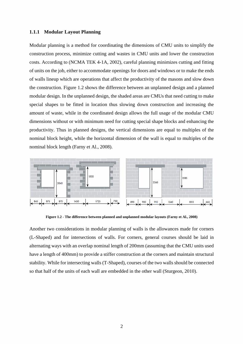
1.1.1 Modular Layout Planning

Modular planning is a method for coordinating the dimensions of CMU units to simplify the

construction process, minimize cutting and wastes in CMU units and lower the construction

costs. According to (NCMA TEK 4-1A, 2002), careful planning minimizes cutting and fitting

of units on the job, either to accommodate openings for doors and windows or to make the ends

of walls lineup which are operations that affect the productivity of the masons and slow down

the construction. Figure 1.2 shows the difference between an unplanned design and a planned

modular design. In the unplanned design, the shaded areas are CMUs that need cutting to make

special shapes to be fitted in location thus slowing down construction and increasing the

amount of waste, while in the coordinated design allows the full usage of the modular CMU

dimensions without or with minimum need for cutting special shape blocks and enhancing the

productivity. Thus in planned designs, the vertical dimensions are equal to multiples of the

nominal block height, while the horizontal dimension of the wall is equal to multiples of the

nominal block length (Farny et Al., 2008).

Figure 1.2 - The difference between planned and unplanned modular layouts (Farny et Al., 2008)

Another two considerations in modular planning of walls is the allowances made for corners

(L-Shaped) and for intersections of walls. For corners, general courses should be laid in

alternating ways with an overlap nominal length of 200mm (assuming that the CMU units used

have a length of 400mm) to provide a stiffer construction at the corners and maintain structural

stability. While for intersecting walls (T-Shaped), courses of the two walls should be connected

so that half of the units of each wall are embedded in the other wall (Sturgeon, 2010).

3

1.2 Masonry Detailing in BIM

1.2.1 Building Information Model (BIM) and Computational Design

Design using computer-aided methods permits faster accomplishment of the tedious and

complex investigations by more flexible study of alternatives. Building Information Modeling

(BIM) is the process of combining all the information that defines a building in a graphical

model; in other words, representing the information database in a graphical form (Eastman,

2011). The core feature of the BIM technology is its reliance on object-oriented parametric

modeling in the representation of building data in relation to its 3D geometry (Azhar et al.,

2008).

There are numerous commercial software providers in the market that use BIM for the different

building construction disciplines. There are some commercial BIM software that can provide

detailing for structural elements such as structural steel and reinforcing steel that can generate

detailed shopdrawings and bar-bending tables. In general, software providers limit end users

to work within the boundaries of the built-in hardcoded commands. However, customizable

data manipulation, relational structures and geometric control is not always possible unless

with a Software Development Kit (SDK) or an Application Programming Interface (API) that

has access to the coding of a BIM software (Autodesk, 2015). Computational Design refers to

the ability to link creative problem solving with powerful and novel computational algorithms

to automate, simulate, script, parameterize, and generate design solutions. Computational

design in BIM offers a way for expanding what can actually be accomplished from the current

BIM tools, by accessing and editing design parameters more effectively, parametric modeling

of building elements or establishing relationships of BIM model elements with almost any

external data/software (Miller, 2014).

1.2.2 Level of Design in BIM

The typical design workflow is to submit increasing Level of Design (LOD) on a number of

consecutive design stages; starting with, conceptual design, schematic design, design

development, contract documents, fabrication/installation drawings (shopdrawings) and

ending with as-built documents. LODs define the degree to which geometries and attached

information has been incorporated in a design stage, which defines the amount of information

project team members may rely on from each design stage. Similarly, each design stage using

BIM is expected to contain more information compared the previous design stage. The LOD

4

of each stage is controlled by a contractual document called “BIM execution plan” so that

building owners and contractors can use the model during the procurement stage, construction

planning stage, fabrication and installation stage, and operational stage of the building. There

is no set standard, industry wide for LODs in BIM. The American Institute of Architects (AIA)

developed a LOD Specification (2013) defining the characteristics of BIM elements at the

different LODs. Since most architects have created in-house standards to control the LODs of

BIM models on their projects, the intent of this document however is to define and standardize

the LOD framework to be used as a communication tool between the project teams (BIMforum,

2015).

1.2.3 Shopdrawings for Masonry

The precision and accuracy of the produced fabrication/shopdrawings is highly dependent on

the technical experiences and competences of the architects/engineers involved in conveying

the design ideology from the design drawings to the shopdrawings with enough level of detail

to ease out the construction process. Moreover, based on the know-how for each trade, they

work on resolving the interrelated issues such as the inconsistent design information, the design

coordination between trades, lack of material take-off sheets, or missing information due to

design changes that were not properly propagated to all the relevant contract documents.

The current practice for produced shopdrawings for masonry lack the amount of detail to ease

out the construction process. Shopdrawings for Masonry are drafted by extracting layouts and

section views from the tender BIM project, where its maximum level of detail would include

the different wall types with the structural layers of each, the surfaces of walls with the texture,

the location of the different inserts and any aesthetic details. The creation of the shopdrawings

would typically include (1) general layout for the location and the components of each wall

and (2) typical off-the-shelf detail drawings for the CMU, its reinforcement and accessories

modeled on the extracted layouts as 2D geometric shapes that excludes any model information

of definitive parameters, which bypasses the features of BIM. This however generates a number

of interrelated problems; where, the quality of the constructed walls is dependent on the know-

how and the expertise of the masons on site which may lead to poor quality control, improper

estimation for the amount of material required from each assembly component for procurement

process, over or under estimation of the amount of waste generated from each assembly

component and inaccurate pricing of change orders.

5

1.3 Problem Statement

Masonry modeling in BIM becomes more challenging when trying to model masonry in the

shopdrawing/fabrication level; which approaches the complexity expected in virtual mockups

to include all required construction details. Such process is labor intensive, time consuming

and less rewarding for Contractors unless there is an automated way to do so (BIM-M, 2016).

In addition, using such tender BIM models in the procurement and estimation process produces

inaccurate material estimates that allows for much assumptions and contingencies, more time

consumed in doing quantity takeoff from the layout drawings with wall-assemblies represented

as 2D geometric shapes and that much construction waste is generated as a result.

1.4 Research Objectives

The global objective of this research is to develop wall-assembly tool that generates full virtual

construction for walls made of CMU in BIM projects and to demonstrate the power of

parametric constraint-based modeling as a technique for the generation and detailing of

building assemblies. The sub-objectives are:

1. Automated generation of virtual mockups for masonry walls in BIM for easy extraction

of shopdrawings

2. Early detection of modular design issues for improved labor productivity and waste

minimization

3. Approaching as-built material quantity takeoff from early project stages for effective

procurement plans

4. Exact calculation of the amounts of cutting and fitting of masonry assemblies for

productivity improvement.

1.5 Scope of Work

The scope of work in this research is limited to the developing of wall-assembly algorithms for

single-wythe masonry walls made from hollow-block units, for straight or curved wall profiles

and with corner connections. The wall components covered under this scope of work are:

CMUs, lintel beams, sill beams, joint reinforcement, vertical reinforcement, wall-to-column

accessories, grout, mortar and top-of-wall to bottom-of-slab joints. However, bond beams,

control joints and irregular wall profiles are not part of the scope of work of this research as

shown in Figure 1.3

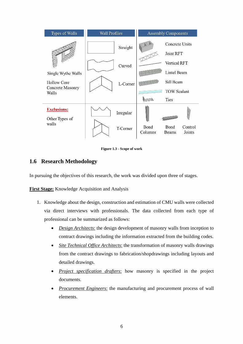
6

Figure 1.3 - Scope of work

1.6 Research Methodology

In pursuing the objectives of this research, the work was divided upon three of stages.

First Stage: Knowledge Acquisition and Analysis

1. Knowledge about the design, construction and estimation of CMU walls were collected

via direct interviews with professionals. The data collected from each type of

professional can be summarized as follows:

Design Architects: the design development of masonry walls from inception to

contract drawings including the information extracted from the building codes.

Site Technical Office Architects: the transformation of masonry walls drawings

from the contract drawings to fabrication/shopdrawings including layouts and

detailed drawings.

Project specification drafters: how masonry is specified in the project

documents.

Procurement Engineers: the manufacturing and procurement process of wall

elements.

7

Quantity Surveyors: the process of quantity takeoff, unit rate estimation and

evaluation of change orders.

2. Review of the literature in areas of BIM for estimation, parametric modeling for

building assemblies and modeling of Masonry with BIM.

Second Stage: Wall-Assembly Model Development

Developing the Wall-Assembly Model based on the information collected in the previous stage

via programming on a commercial parametric modeling software for modeling building

assemblies. Autodesk® Revit® was used as the BIM environment, designscript® was used as

the visual programming language and Dynamo® as designscript® compiler.

1. Designing Revit® Families with types for CMUs, lintel beams, sill beams, joint

reinforcement, vertical reinforcement, wall-to-column accessories, corner connections

and top-of-wall to bottom-of-slab joints.

2. Developing a number of 19 wall-assembly algorithms working in parallel and in series

under one model, including:

2 algorithms for the detection of wall parameters and profiles from a Revit®

model using designscript®

8 algorithms for the construction of each of the abovementioned wall

components using designscript®

9 algorithms for quantity takeoff of each component including cut lengths using

designscript®

Third Stage: Model Validation and Analysis

Validation of the developed wall-assembly algorithms and model using an actual industry case

study to demonstrate and compare the outputs from each and highlight the developed

algorithms features and efficiency.

1.7 Thesis Organization

This dissertation is organized into 5 chapters; this section summarizes the contents of each

chapter:

Chapter 1 – Introduction: provides a general introduction on masonry walls, covering a

breakdown for the components, terminologies, modular planning and layout. Followed by an

8

introduction to Building Information Models, computational design and parametric modeling.

Then, the problem statement, research objectives, scope of work, research methodology and

thesis organization.

Chapter 2 – Literature Review: provides an in-depth review of literature in the state-of-art

developments in areas of BIM, the uses of BIM in estimation, parametric modeling for building

assemblies and modeling of masonry with BIM, followed by the conclusions from the literature

review.

Chapter 3 – Methodology and Model Development: discusses in details the information

collecting phase followed by in depth discussion on the development of the wall-assembly

model by demonstrating the features of the newly introduced algorithms that serve the purpose

of the research objectives.

Chapter 4 – Cases Study and Validation: validating the outcomes generated from the newly

developed algorithms on an actual case study comparing the results from the case study with

the results from the wall-assembly model.

Chapter 5 – Summary, Conclusions and Recommendations: summarizes and concludes the

research and provides recommendations for future development and research in the area of

parametric modeling of building assemblies.

9

2. CHAPTER 2 – LITERATURE REVIEW

BIM has been around for over two decades; however, it just started to become very popular at

the turn of the century. Praised by the construction industry, BIM proved that it has the potential

for developing and revolutionizing design and construction assistance in the Architecture,

Engineering and Construction industry (AEC). Since the literature review for the application

of BIM in the AEC industry is huge, this chapter focuses particularly on four main areas that

support the context of this research as shown in Figure 2.1, and can be summarized as follows:

Figure 2.1 - Areas of concern under this chapter

1. The extent to which AEC companies are adopting the BIM technology compared to the use

of traditional methods in both the design and construction phases, including its reported

uses, benefits and barriers

2. The productivity and accuracy achievements attained using the BIM technology in quantity

takeoff, estimation and procurement compared to the traditional estimation methods

3. Attempts and developments in the generation of building assemblies using parametric and

generative modeling techniques

4. Attempts and development in the modeling of masonry structures/walls using BIM.

BIM

Use, Benefits and

Barriers

BIM

Estimation and

Procurement

Parametric

Modeling

Building

assemblies

BIM &

Parametric

Modeling

Masonry

LITERATURE REVIEW

10

2.1 BIM uses, benefits and barriers

This section aims to explore the extent to which companies and projects adopt BIM; together

with providing insight on how companies perceive the functions and objectives of using BIM

compared to the traditional methods and to highlighting previous success and fail case studies

from actual construction projects that have adopted BIM during their design and construction

phases.

A number of surveys were conducted throughout the literature to assess the way the industry,

adopts BIM, including to what extent are the adoption measures, the technology’s benefits and

barriers. Azhar (2008) conducted a survey to track the productivity gain from the use of BIM

in construction projects. The main target of the survey was the use of BIM in construction

management from medium-sized to large architecture/engineering firms. The results

demonstrate that adopting BIM compared to the traditional methods has resulted in

productivity gain, ranging from 20% to 30% more compared to the use of CAD or the

traditional methods in preparation and issuing of construction documents. It was also concluded

that the application of BIM during construction phases has reduced the amount of Request for

Information (RFI) and change orders almost ten times less compared to the use of traditional

methods.

Another survey was conducted by Yan and Damian (2008) for about 70 individuals from the

AEC industry in both the US and UK on BIM adoption, perceived benefits for companies, and

perceived barriers in adopting this technology. The results from the survey concluded that

adopting BIM technology has provided firms with a number of benefits compared to the

traditional methods. (1) BIM helped in reducing the abstraction and integrated multiple

disciplines together during the design and documentation phase; thus minimizing design errors,

fixing coordination issues, and providing a collaboration environment between the different

project stakeholders. (2) In terms of productivity improvement, adopting BIM has saved the

cost of design due to early detection and fixing of design issues from early project stages. And

(3) in terms of site works, BIM helped in reducing the use of engineers in site offices that

convert design drawings to fabrication drawings, thus saving indirect costs for contractors

during the project lifecycle. However, for the barriers, companies have to allocated time and

cost for the training of its resources to use this technology and there will be mostly social

habitual resistance to such change as most clients, architects and contractors are already

11

satisfied with the traditional methods of design and delivery of their projects without the need

for a newer technology.

A study by Becerik-Geber and Rice (2010) tackled another issue which was not covered in

previous surveys, which is the way companies perceive the BIM technology. The survey

targeted only AEC firms in the US, the survey results were summarized as shown in Figure

2.2. The results from the survey highlight that the top use of BIM is project visualization; still

companies treat BIM as a 3D tool to visualize the form of buildings without fully understanding

the potential of information inside the model. The second uses of BIM are both clash-detection

and building design. AEC companies use BIM to design projects and then resolve the major

coordination issues between the different design trades when compiling models together into

one multi-model. The list goes on; however, it can be denoted that the use of BIM for building

assemblies and for model-based estimation has still not fully ripe yet.

Figure 2.2 – The top uses of BIM in the US AEC industry (Becerik-Geber, 2010)

Following the work of previous researchers, Hergunsel (2011) conducted two studies. The first

was to classify the types of BIM as mostly used by AEC companies. The second survey was to

explore the available BIM authoring and construction management tools in the market. The

first study concluded that companies perceive the BIM technology in different ways, and can

be classified as shown in Table 2.1. The study shows that there are mainly four types of BIM

as used by AEC companies, out of which, Social BIM and Intimate BIM are the most

promising.

12

Table 2.1 - The understanding of BIM by companies in the industry (adopted from Hergunsel, 2011)

Types of BIM Explanation

Hollywood BIM The contractor creates and uses the BIM model for producing only high

quality 3D renderings with no further use of the built-up information of the

model.

Lonely BIM The model is practiced internally only within a single organization and not

shared with the rest of the organization.

Social BIM A collaborative type of BIM in which the model is shared between the

engineer, architect, contractor and sub-contractors. Could be used to create

constructability analysis reports, coordinate, plan site activities, generate

schedules and cost estimates.

Intimate BIM A type of BIM-enabled integrated project delivery in which the contractor,

design team and the owner contractually share the risk and reward of the

project.

The second survey conducted by Hergunsel (2011) highlight that there are numerous BIM

software packages currently available in the market. Table 2.2 highlights some of the most

popular BIM packages by most AEC firms, including their primary function and the discipline

they serve.

Table 2.2 - Most popular BIM authoring tools and construction management tools

(adopted from Hergunsel, 2011)

Product Name Manufacturer Primary Function

BIM Authoring Tools

Revit Architecture Autodesk 3D Architectural Modeling and Parametric Design

Revit Structure Autodesk 3D Structural Modeling and Parametric Design

Revit MEP Autodesk 3D detailed MEP modeling

AutoCAD Civil 3D Autodesk 3D site development and infrastructure including

parametric design

Bentley BIM Suite Bentley 3D Architectural, Structural, Mechanical, Electrical

and Generative components modeling

Power Civil Bentley Site Development

13

ArchiCAD Graphisoft 3D Architectural Modeling

MEP Modeller Graphisoft 3D detailed MEP Modeling

Tekla Structures Tekla 3D Detailed Structural Modeling

Vico Office Vico Systems 5D Modeling, can generate cost and schedule data

BIM Construction Management Tools

Navisworks

Manage

Autodesk Clash Detection, 5D Scheduling, Animation,

Rendering

ProjectWise Bentley Clash Detection, 4D Scheduling

Synchro Synchro Ltd. 4D Planning and Scheduling

Tekla Structures Tekla 4D for structure-centric models

Vico Office Vico Systems Coordination, scheduling, Estimation

The survey results concluded that most companies use Autodesk products (Revit Architecture,

Structure, MEP and Navisworks) and Graphisoft ArchiCAD products.

A study conducted by Bryde et al. (2013) explored the pros and cons generated from utilizing

BIM on a number of 35 different type construction projects worldwide reported from literature.

The criteria by which the pros and cons were assessed was the utilization of BIM in (1)

coordination, (2) scope of work, (3) time control, (4) cost control, (5) quality control, (5)

organizational management, (6) communication management, (7) Risk management and (8)

software issues. The results from the study can be summarized as shown in Figure 2.3. The

results conclude that some projects have reported negative instances in the software issues

criterion, particularly in interoperability issues between different software for design and

analysis, highlighting its negative impacts against enhancing collaboration between the

different project stakeholders; as well as, software were unable to handle large amount of data

inside models with complex geometries and elements. The most frequently reported benefit

however was in cost reduction, managing the construction costs of projects in general, model

based quantity takeoff and estimation and change orders management.

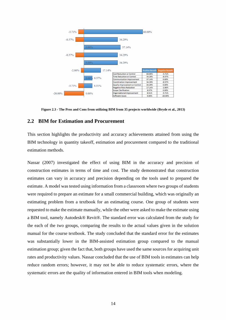
14

Figure 2.3 - The Pros and Cons from utilizing BIM from 35 projects worldwide (Bryde et al., 2013)

2.2 BIM for Estimation and Procurement

This section highlights the productivity and accuracy achievements attained from using the

BIM technology in quantity takeoff, estimation and procurement compared to the traditional

estimation methods.

Nassar (2007) investigated the effect of using BIM in the accuracy and precision of

construction estimates in terms of time and cost. The study demonstrated that construction

estimates can vary in accuracy and precision depending on the tools used to prepared the

estimate. A model was tested using information from a classroom where two groups of students

were required to prepare an estimate for a small commercial building, which was originally an

estimating problem from a textbook for an estimating course. One group of students were

requested to make the estimate manually, while the other were asked to make the estimate using

a BIM tool, namely Autodesk® Revit®. The standard error was calculated from the study for

the each of the two groups, comparing the results to the actual values given in the solution

manual for the course textbook. The study concluded that the standard error for the estimates

was substantially lower in the BIM-assisted estimation group compared to the manual

estimation group; given the fact that, both groups have used the same sources for acquiring unit

rates and productivity values. Nassar concluded that the use of BIM tools in estimates can help

reduce random errors; however, it may not be able to reduce systematic errors, where the

systematic errors are the quality of information entered in BIM tools when modeling.

15

Grilo and Goncalves (2010) developed a framework that describes how BIM combined with

Model-Driven Architecture, Service Oriented Architecture and Cloud Computing can be

integrated to be used as an e-procurement platform in the AEC industry. Their application faced

some difficulties in the ability of the model to convert individual building objects in aggregate

products to be released for tender; moreover, the level of aggregation in BIM objects tend to

be very elementary and that tender focus more on aggregate levels of products and services. In

other words, quantities can be easily obtained from BIM but to organize the elements to be

tendered is rather complex.

Firat et al. (2010) examined the interface between the quantity take-off performed during the

design stages versus the quantity take-off performed during the construction stage. The

efficiency of the take-off lies in the transfer of information from the design process to the

construction process. The authors highlight that the existing BIM tools facilitate the quantity

take-off to be performed during the design phases of the project; however, during the

construction stage, more details are required to be modeled by the contractor. A model-based

system was proposed which is Building Construction Information Model (BCIM) that should

work during the construction phase of the project, where data about project element should be

stored, updated and reused. BCIM is composed of three sub-models: (1) a model that provides

sections and quantities, (2) resources and cost model that generates activity lists and labor

productivity for duration calculation and (3) process model that includes the interdependencies

of activity. The model was tested on two cases studies demonstrate the feature of BCIM. The

results show that the largest obstacle to BCIM is the lack of modeling guidelines. Models in

the designs stage are mostly designed to generate the form of the building without the

allowance for the construction details. For example, floor slabs have been drawn in design

models as one complete slab regardless of its floor area; however, slabs from the contractor’s

perspective have to be disjoined with expansion joints. This amount of detail is not present in

the designers’ models which is considered as an obstacle to the application of BCIM. The study

concludes that for quantity-takeoff to be made easy and efficient, the level of detail for models

have to be agreed upon by all participants involved in the project.

16

Montero et al. (2013) conducted a survey on how BIM could be used for quantity takeoff

(QTO) compared to the conventional CAD quantity takeoff. The research reported that the

process of QTO is not straightforward, the model has to be adapted to optimize the takeoff

process since it may generate conflicts and errors due to the model design is not takeoff ready.

Most BIM tools have the takeoff feature; however, they are unable to manage the data for a

proper accurate QTO. Thus, it is essential to use a structured system of IDs and layers inside

the model to ensure consistence of the takeoff process. The research concludes that the

approach to designing models has to change in order to be used in QTO, frameworks and

standards have to be developed and structured to optimize the performance of the BIM tools in

providing a guaranteed consistent QTO.

Lee et al. (2013) proposed a methodology that automatically infers the most appropriate work

items suitable for building elements and materials on the basis of work conditions using

semantic technology. The objective of this methodology is to improve the accuracy of BIM-

based QTO compared to the conventional QTO to BIM tools. The proposed methodology

consists of three steps: (1) BIM data are extract into IFCXML and then converted into a

machine-readable format (RDF), (2) a reasoning algorithm creates inferred knowledge with the

work items by means of reasoning, and finally (3) the query engine retrieves relevant

information related to the inference of the work item using expert knowledge. The

methodology was validated on a case study project, results demonstrate that the process

contributes to the full automation of cost estimation and improve the reliability and accuracy

of the estimation results as well as assisting cost estimators to extract more BIM data easily.

Choi et al. (2014) proposed a methodology to improve the reliability of the QTO from BIM

during the early design stages of the project. The methodology works on four stages: (1) BIM

modeling for schematic estimation, verification to increase the accuracy of the QTO,

verification of the data for estimation, extract quantities and provide estimation. The developed

prototype named InSightBIM-QTO. However, the application of the study was limited to

concrete frame elements only, further research is required to fully test the solution.

Elbeltagi et al. (2014) proposed a methodology for visualizing and evaluating the construction

performance with respect to cost using a BIM based system. Their proposed model enabled nD

visualization of the construction progress with the geospatial conditions. The proposed model

could provide the users with the capability of visualizing the actual cost expenditures for the

17

different building elements and compare it with the budgeted costs throughout different time

intervals.

Nour et al. (2015) introduced an approach for configuring the exterior envelop of buildings by

selecting and allocating elements and material by assigning them with certain locations on a

buildings envelop with the objective of optimizing the life cycle cost. The working principle

of their model is that external building components such as façades and roofs are segmented

into independent objects in a BIM project. Genetic Algorithms optimization coupled with

industry foundation classes and an energy simulation tool is then applied. The benefits from

using this model is that an optimal configuration of a buildings energy saving elements can be

achieved that that allows for a positive return on investment as well as eliminating the use of

any unnecessary energy saving elements that does not show any reduction in the life cycle cost.

2.3 Parametric Modeling of Building Assemblies

Object-oriented parametric modeling is the core of the BIM technology. The term “parametric”

describes the process where elements in an assembly or model maintain mathematical

relationships controlled by a set of parameters in which any modification to an element

automatically adjusts attached elements to maintain the established relationship. This section

explores the attempts and developments of modeling building assemblies using object-oriented

parametric modeling. Parametric modeling originated in the mechanical engineering industry,

however from early attempts to use parametric modeling in the AEC industry was not until the

early 90s.

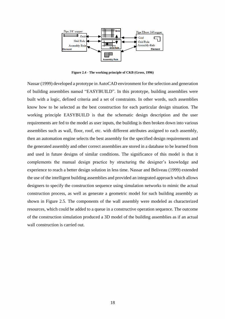
Gross (1996) presented a prototype CAD program named construction kit builder (CKB) that

supported rule-governed layouts for the design of building elements. The significance of CKB

is that it enabled the designer to program the positioning and the assembly rules for a layout of

building elements. This was done by specifying layout grids, rules for placing elements relative

to the layout grids and relative to one another as shown in Figure 2.4. For example, if a designer

was required to generate a piping assembly, then by selecting the two elements, the pipe and

the pipe elbow, CKB generates the assembly and provides the placement location on the layout

grid line and zone using the coded grid and assembly rules.

18

Figure 2.4 - The working principle of CKB (Gross, 1996)

Nassar (1999) developed a prototype in AutoCAD environment for the selection and generation

of building assemblies named “EASYBUILD”. In this prototype, building assemblies were

built with a logic, defined criteria and a set of constraints. In other words, such assemblies

know how to be selected as the best construction for each particular design situation. The

working principle EASYBUILD is that the schematic design description and the user

requirements are fed to the model as user inputs, the building is then broken down into various

assemblies such as wall, floor, roof, etc. with different attributes assigned to each assembly,

then an automation engine selects the best assembly for the specified design requirements and

the generated assembly and other correct assemblies are stored in a database to be learned from

and used in future designs of similar conditions. The significance of this model is that it

complements the manual design practice by structuring the designer’s knowledge and

experience to reach a better design solution in less time. Nassar and Beliveau (1999) extended

the use of the intelligent building assemblies and provided an integrated approach which allows

designers to specify the construction sequence using simulation networks to mimic the actual

construction process, as well as generate a geometric model for such building assembly as

shown in Figure 2.5. The components of the wall assembly were modeled as characterized

resources, which could be added to a queue in a constructive operation sequence. The outcome

of the construction simulation produced a 3D model of the building assemblies as if an actual

wall construction is carried out.

19

Figure 2.5 - A simulation network for a partition wall assembly (Nassar and Beliveau, 1999)

Sacks et al. (2004) presented framework to shift from the traditional 2D drafting to 3D top-

down parametric modeling of precast building elements. The framework also allowed for the

automated generation of shopdrawings which holds potential to eliminate most of the drafting

sources errors. The framework was tested on a number of seven case studies for projects that

deploy the use of concrete precast elements in their construction. A number of outcomes were

generated, including: the use of parametric modeling in the logical relationships between the

precast elements has maintained integrity of the elements and minimized the designers’

intervention thus reducing errors, automated detailing of the hardware connections remove the

probability of human error in the misplacing and incorrect selection of the hardware itself and

the use of 3D building model provided a platform for automated design check routines which

improved the process of design checking.

Niemeijer et al. (2009) developed a methodology for architects to assist in mass customization

of buildings using a set of designed customizable constraints. The idea was to allow the

involvement of house owners in the design stage, while providing a control measure to ensure

the validity of such customized designs using parametric constraint-based modeling. Since

house owners were involved in the design process, an easy user interface was required; the

authors used a “puzzle piece” programming syntax where each puzzle piece represents part of

20

a sentence which when placed in series as shown in Figure 2.6, form a sentence read by the

house owner as a customization in the design while by the program itself as a manipulation the

design itself.

Figure 2.6 – The puzzle piece syntax (Niemeijer et al., 2009)

The leap in using this syntax however is that the evolvement of building owners to customize

their design is based on constructing simple sentences where each word is a puzzle piece and

is coded with a parametric model. The architect could after creating the initial design provide

a set of alternatives with constraints to the designed building elements; the end-user on the

other hand could customize the design based on the defined set of alternatives while the

designer assuring that the predefined set of constraints are satisfied as shown in figure. It was

concluded that this prototype reviled its effectiveness on small scale projects; however, on large

scale projects this would be a tedious design job for the architect to define a set of design

alternative for each assembly. Niemeijer et al. (2010) extended their work to allow the

incorporation of the design information from a BIM package and perform the constraint check

requirements using its Industry Foundation Class (IFC) file. This was possible by creating a

prototype where constraints could be specified and checked using the imported IFC

information. Their study concluded that such incorporation for constraint modeling and

checking with IFC files was not very practical since IFCs were not designed for constraint

checking but for storing building models’ information only, thus architects need to infer some

parameters from building elements such as texture of material, durability, etc.

Cabecinhas (2010) developed a programming language named “Visual Scheme” based on

AutoLISP syntax which was intended to be a computational design language for architects.

The motive behind the development was that architects require the use of parametric variables

to flex their designs until its full development. However, computational programming using

text-based languages for architects have proved to be a difficult approach to adopt since it

generates short feedback loops in the event of model flexing and model testing. Visual Scheme

21

language provide interoperability features between the programming interface and the

visualization program. Its working principle is that a tree of high dimension geometric

primitives and operators are computed inside the core of the program and then passed to the

back-end of visual scheme, this computation is presented on the canvas interface of the

visualization program.

Another study by Veliz et al. (2011) worked on testing the practical uses of a constraint-based

design system on a commercially widespread software like Autodesk® Revit® 2011 without

the need of text-based programming. During a floor plan design, constraint-based parameters

were added for each space. Parameters were constrained with maximum and minimum values

to represent the possible allowance for the dimensions of the space being designed. what is

interesting about this model is that it allows designers explore one or more design solution

based on the set of constraints defined for each space as shown in Figure 2.7. The model was

effective on small scale examples; however, this model was not tested for more complex

parameters and models.

Figure 2.7 - Generation of two different design alternatives based on defining constraints for floor spaces (Veliz et al.,

2011)

Bernal and Eastman (2011) studied the degrees of complexity which entail a high amount of

the designers’ expertise in the design activities, from inception phase up to the final stages of

the design with the highly constrained solutions space. They developed a system that uses a

top-down approach for design of nested assemblies and custom functions to be embedded in

reusable parametric objects. The study was conducted on the service cores of buildings to be

the parametric objects. The outcomes of this approach demonstrated that the building core, as

a parametric object to the design, adapts to the changes done during the design formulation

stage which acts as a feedback for the architect about the design intent and the decision making

process.

22

Bonev and Hvam (2012) proposed a framework for the use of a knowledge-based geometric

modeling approach in the automation routine manufacturing tasks for precast concrete

elements. The framework automates the modeling of the precast elements, provided with the

knowledge of the experts to improve the efficiently of the overall process compared to the

manual manufacturing process per element. The developed system was based on iLogic®

software, an integrated system of CAD and expert system, which would allow the designer to

use templates containing information pertaining the shape and specifications of the required

precast element to be designed and manufactured. Therefore, the design of precast assembly

elements could be enhanced with the automated generation of production drawings and that

the assembly design would be stored in the product data management system to be used again

for further production. The study concluded that such system was very much effective on the

manual routine design tasks of each precast element. However, non-routine designs with

complex geometries might require a high degree of parameters and information to be specified

by the designer.

Fai et al. (2013) investigated the advantages, limits and challenges that follow the use of BIM

for the documentation of old structures via presenting the concept of Historic Building

Information Model (HBIM); which can be used in rehabilitation and restoration projects of

historic structures. HBIM offers a library of parametric building objects such as column

capitals, column shafts, etc. that follow the proportional rules of the classical architecture which

date back to the 19th century and is considered an essential tool for modelling elements of

classical and neoclassical buildings. In their paper a case study was presented as an application

to document the roofing structure of Canada’s Commissariat Building that includes the

Parliament precinct and eight lock stations that connect the Rideau Canal to the Ottawa river.

A survey was carried out using a number of surveying equipment and hand calculations to

determine the components of the roofing structure for the building. Because the roof was

basically a truss, it was possible to create a parametric assembly by modifying parameters in a

basic truss family type to mimic the actual constructed truss inside the building as shown in

Figure 2.8.

23

Figure 2.8 - (left) generated roof structure after survey, (right) generated roof elements assembly stored in HBIM

(Fai et al., 2013)

The results from the study demonstrate that HBIM can be used to document the design and

construction of the historic building assemblies. Moreover, HBIM could be used as a library to

generate shopdrawings or fabrication drawings that could facilitate the rehabilitation of such

projects, where governments can benefit the restoration, conservation and management of

heritage buildings.

Manrique et al. (2015) explored the integration between mathematical algorithms, parametric

and 3D modeling to efficiently deliver optimal construction/shopdrawings for wood framing

designs. A model was developed on VBA to formulate the parametric equations and was then

integrated with AutoCAD environment to import the geometry information. The working

principle of the model was that, any wall object is broken into a number of panels with lengths

specified by the user, which is in accordance with the type of equipment and the method of

transport that will be adopted by the building contractor facilitate the construction. The

algorithm then evaluates the framing method and the given structural requirements to generate

shopdrawings, material takeoffs and cutting lists in a manner which minimizes material wastes.

The produced shopdrawings and cultists could then be used to build the required panels in a

manufacturing shop, then the panels could to be shipped to the construction site for assembly

and installation. The purpose of their model was to automatically generate shopdrawings for

either the construction components or for overall layout shopdrawings. Thus, all relevant

requirements could be obtained from the produced shopdrawings including material quantity

takeoff and assembly plans. The outcomes presented highlight the considerable amount of

hours that could be saved by the onsite technical office team in the generation of shopdrawings

and thus minimizing a contractor’s overhead costs.

24

2.4 Parametric Modeling of Masonry using BIM tools

In concurrent with the previous section about the modeling of building assemblies using object-

oriented parametric modeling, this section explores attempts to model masonry walls as a

building assembly with parametric components.

Scheer et al. (2008) highlighted the possibility of developing an object-based BIM tool for

masonry walls in order to facilitate the representation of constructive details and contribute the

quality control on construction sites. The authors highlighted that there are two approaches for

the development of such tool; either a stand-alone application or an associate application, were

it is recommended to use an associate application. The main difference between each of them

is that a stand-alone application can offer flexibility in integration with multiple BIM software;

however, this may require enormous amount of time in its programming to ensure integration

with multiple formats. On the other hand, an associate application which would be developed

for a specific BIM software focuses on the main functions of automation of masonry design

not on the coding itself; however, the lack of flexibility in its integration with other software

would demand new programming for each BIM software to be used in. The authors suggested

that in order to develop a masonry assembly tool (assuming top-down modeling approach), the

following needs to be included: (1) native parametric objects (e.g. wall elements) in BIM that

can be embodied with intelligence to behave as a composition of blocks or bricks, (2) templates

that included a standard for graphic representation such as bond pattern, coursing and coatings,

(3) special parametric objects which are the masonry wall elements, (4) scripts and macro

which are tools that automate the process of assembling masonry units through a routine of

algorithms that trigger BIM functions, (5) association with databases to allow the querying of

attributes from objects such as area and volume, and (6) API that allows communication with

the core functions of a BIM. The authors suggested the following framework that could be used

to automate the generation of masonry wall assemblies as shown in Figure 2.9. The framework

demonstrates that with the use of specialized parametric objects such as CMUs and the use of

a graphics processing engine could generate graphic instances of a wall embodied with blocks

or brick units

25

Figure 2.9 - Suggested framework for the generation of masonry wall assemblies, Scheer et al. (2008)

Monteiro et al. (2009) discussed the implications of developing a masonry wall assembly. This

was classified into two representations, explicit and implicit. Explicit representation means the

construction of the assembly using parametric object families while the implicit representation

means using the concept of generative modeling in the construction of the assembly without

degrading the handling performance of a BIM. In their study both experiments were performed

in Autodesk® Revit® Architecture 2010.First, the implicit representation experiment proposed

that wall elements will not be modeled, instead they will be automatically created with a special

wall family that incorporates the representation of blocks by parametric means. However, this

was not applicable since walls are system families in Revit® and system families cannot be

created or edited. Moreover, generative modeling technique was used by the representation of

shape rules and vocabulary that translate expressions to a 3D graphical representation which

however could not provide the complex masonry representation needed. In the explicit

representation experiment however, a concrete block family was designed in Revit® family

editor and loaded into a project. The masonry family was designed with a set of parameters

that define the dimension of the block in accordance with a specification from a traditional

Brazilian Concrete block manufacturer. The family template used to create the block was

“Metric Generic Model Wall Based.rft” which is used to create families instantiated only within

walls. In order to place blocks inside walls, a formula was placed inside the family editor for

the masonry units which generates a parametric array based on the wall length and height

parameters as shown in Figure 2.10. However, the model had a set of limitations, the parametric

array formula generated extra course of blocks that had to be manually removed, no allowance

was made for blocks of other sizes to cope with the non-modular wall dimensions, they had to

be placed and arrayed manually, moreover, the model was not automated are required much

human intervention in the process.

26

Figure 2.10 - Creating formulas that generate parametric rectangular arrays in the masonry family editor from

querying the Revit wall length and height parameters (Monteiro et al. (2009)

Cavieres et al. (2011) presented a study that explores the potential of using parametric modeling

to embed design and construction knowledge in the form of generative rules and feedback rule

checking functions that provide timely evaluation of design alternatives. The authors used

concrete masonry as an application to their model, since concrete masonry components can be

modeled by parametric equations using an existing parametric CAD system from Bentley®

called Generative Components. The working principle of the model proposes a generative

approach based on a library of pre-defined parametric templates that allow modeled concrete

units to be positioned and adapted automatically as the design changes. The developed model

relies on a hybrid system of parametric and non-parametric modeling tools, where (1) a

designer creates a surface as in a conventional 3D CAD environment then a discretized surface

inside the big surface is generated resemble the masonry units and the shape of the bond. Then

(2) a component-based model is adopted that selects the pre-defined parametric masonry

objects where automatic placements of masonry blocks are done by iterative propagation in a

bottom-up manner. the uses of such model facilitates the top-down decomposition of a wall for

simplified structural analysis, feedback function checks for the evaluation of cross section

eccentricity of blocks and loads to verify allowable stresses and the recommends back values

for the layout of the blocks and provide a selection for the positioning and diameter of steel

rebar. The working principle of the model can be shown in Figure 2.11.

27

Figure 2.11 - Working principle of the model (Cavieres et al. (2011)

Their study concluded that with the aid of parametric modeling, their system can provide

constructability guidance to architects before they seek the advice of the structural engineer or

the contractor. This was done by embedding the structural knowledge inside the modeling of

the masonry units. The objective was to provide insight for architects to explore design

alternatives of irregular shaped masonry walls structurally and in terms of constructability.

Gentry et al., (2014) presented a study on the potentials of and requirements for BIM modeling

of masonry via presenting three case study projects that were constructed with masonry;

highlighting that a masonry tool in BIM need to be developed to model masonry assemblies

parametrically. Their study proposed that a BIM tool that models masonry has to (1) define

high-level classes for masonry; including methods for generating objects, bond patterns,

openings, etc. (2) identify rules that define the relationships between objects; such as how the

bonding pattern will react to wall inserts, (3) strategy to adapt to modularity, and (4) an

interface that allows defining and importing the masonry units. The study concluded that the

use of BIM for modeling masonry assemblies can improve the constructability issues, and

contribute to the checking for the modularity of the designed walls before construction.

Sharif and Gentry (2015) developed a database model for masonry units called Masonry Unit

Database (MUD) with the objective of providing a data structure framework that stores the

required data for digital representation of masonry units to be used in BIM projects. This

developed database could be used for designers to incorporate up to date masonry product

information to their projects. The development of MUD required units to be defined as Building

28

Object Models (BOM) first, where 2D and 3D geometries can be modeled as parametric

geometry. The data structured in MUD included a number of attributes about the masonry units;

geometry, material, physical properties, color, texture, manufacturer, supplier, etc. MUD was

designed as a relational SQL database that can be accessed in Autodesk® Revit® using

Dynamo® plugin for Revit®, which is a visual scripting language that has access to Revit®

databases. The working principle of MUD is that it is a web-based service where manufactures,

suppliers and data managers access the MUD website feeding the database with information

pertaining their products, the information is then structured in MUD central database, finally

the data outputs can be used either for the MUD website or imported to Revit® via Dynamo®

as shown in Figure 2.12.

Figure 2.12 - Masonry units imported to Dynamo® interface via MUD script that can be then exported to Revit®

(Sharif and Gentry, 2015)

29

2.5 Literature Conclusions

Previous works conclude that BIM improves the productivity of the works by almost 20% more

compared to the traditional methods (Azhar, 2008); moreover, BIM provides collaboration

between the different project stakeholders and minimizes abstraction and design errors.

Moreover, BIM can reduce the overall costs of the project by deploying less resources and

provide robust control of the built project (Azhar 2008, Yan & Damien 2008). The top usage

of BIM among AEC firms and projects are visualization, building design and design

coordination (Becerik-Geber & Rice 2010, Hergunsel 2011). There are numerous BIM tools in

the market either authoring tools or construction management tools. Autodesk® Revit® and

Graphisoft® ArchiCAD® are the most commonly used in the market (Hergunsel 2011).

BIM also enhances the process of quantity takeoff and estimation compared to the traditional

methods; however, models need to be designed to be takeoff-ready. Design guidance and rules

to model building assemblies are also required to allow BIM models to be takeoff-ready and

could be used in lifecycle costing and cost monitoring. It is worth noting that BIM can resolve

the accuracy errors in the takeoff process and not the systematic errors (Nassar 2007, Firat et

al. 2010, Montero et al. 2013, Choi et al. 2014, Elbeltagi et al. 2014 and Nour et al. 2015).

Parametric modeling is the core of the BIM technology, there are numerous amount of literature

on the attempts and developments of modeling building assemblies using different parametric

modeling tools and techniques. Constraint-based modeling can be used in detailing building

assemblies using a set of parametric relationships and equations. As the design level progresses,

parametric building assemblies allow the designer to have more control over the model as well

as generate design alternatives which automatically updates during design flexing. Parametric

geometric assemblies can be fed with knowledge and know-hows from experts and

professionals to create knowledge-based geometric assemblies that can be used in generative

BIMs, repetitive tasks can be automated by the generation of nested building assemblies which

can be used in different types of applications such as manufacturing and automated

construction drawings production (Nassar 1999, Nassar & Beliveau 1999, Sacks et al. 2003,

Niemeijer et al. 2009, Bonev & Hvam 2012, Fai et al. 2013 and Manrique et al. 2015). The use

of visual programming languages is more robust in computational design compared to text-

based coding languages. Moreover, parametric assemblies can be designed on different

widespread commercial software for easy implementation and integration with industry case

studies (Cabecinhas 2010 Velize et al 2011 and Bernal & Eastman 2011).Developing an object

30

based BIM tool for masonry walls can facilitate the visualization of the construction details as

well as contribute to the quality control during the construction process. such tools could be

developed as standalone applications or integrated applications; however integrated

applications are more recommended since the focus will be on the automation of the building

assembly not on the coding and interoperability with other software. Masonry units can be

modeled as parametric arrays in both the horizontal and vertical directions and require a native

object to be stacked on. Unfortunately, masonry modeling requires user intervention in the

modeling process and there is no tool to date that could automate the generation of masonry

assemblies with all its components. The recommended approach for modeling masonry

assemblies for future work is to use top-down modeling since the native objects

(walls/surfaces) are originally supplied with the BIM models and they will require breakdown

into the different assembly elements (Scheer et al 2008, Monteiro et al 2009 and Cavieres et al

2011).

Thus the aim of this research is to tackle the gaps found in the previous works by developing a

series of new algorithms using parametric modeling techniques that automatically generate

masonry wall assemblies with all its components via converting the native BIM model wall

elements into detailed wall elements.The outputs from these algorithms can have multiple uses,

including: the automatic generation of detailed shop drawings for walls made of CMU

assemblies, actual unit rate estimation for the walls of the building, actual material estimation

to plan for procurement, exact amount of waste expected to be generated during actual

construction.

31

3. CHAPTER 3 – MODEL DESIGN AND VERIFICATION

The work on this research is divided into stages. First, the data collection stage where direct

interviews with design architects, technical office architects, specifications drafters,

procurement engineers and cost estimators were conducted. Second, development of the new

wall assembly algorithms based on the information collected from the previous stage, design

manuals, building codes and the literature review. Finally, validation of the wall assembly

algorithms using an actual case study to demonstrate the model capabilities essential features

and limitations as shown in Figure 3.1.

Figure 3.1 - Research Methodology Stages

3.1 Stage 1 – Knowledge Acquisition: Direct Interviews

3.1.1 Sampling

The aim of this stage was to identify some information pertaining the design and construction

of blockwork. Face to face interviews took place with a number of 23 interviewees from the

AEC industry. The sample of interviewees included professionals in the both engineering and

contracting fields. The interviews took place in August 2015. Before the interview, the

interviewees were reassured of the confidentiality of their identities and their organizations.

After the consent of the interviewees, a transcript of their responses was written down. For this

research, all interviewees have direct work experience and exposure in the phases of building

design, tendering and construction.

1. Knowledge Aquistion

• Direct interviews with industry professionals

• Design Manuals

• Building Codes

2. Model Development

• Modeling of wall elements

• Wall assembly algorithms development

• Algorithms pilot testing

3. Validation and Results

• Industry case study application

• Results and Conclusions

32

3.1.2 The Interview Sessions

The interview sessions were about 30 minutes with each interviewee and were conducted on

different dates, depending on the available timeslot from each interviewee. Each interviewee

was provided with the list of questions and an open discussion was held. After the interviews

were completed, some interviewees provided sample shopdrawings, detailed drawings,

specifications, and BIM projects to complement their statements.

The research topic and its significance were presented to each interviewee. The interview type

was semi-structured with predetermined list of questions. The questions were intended to

discuss one area of the topic; however, spaces for informal discussion were given in order to

obtain more information. Moreover, open ended questions were used which resulted in a wider

range of answers from the interviewees. A list of the used questions in the interviews is

documented in Appendix 1.

The following Table 3.1 presents the list of interviewees, their positions, years of experience,

the type of firm they work for and the areas of discussion.

Table 3.1 - List of interviewees and the areas of discussion

Cat. Positions Years of

Experience

Type of

Firm Area of Discussion

Des

ign D

evel

opm

ent

Sta

ge

vs

Shopdra

win

gs

Sta

ge

Project

Manager 20+

Engineer

(1 no.)

The issued for tender LOD

drawings for masonry walls

The use of BIM in the design

phase

Components for masonry wall

drawings including the reference

to typical details

References to building codes and

standards

The transformation from the

design drawing to shopdrawings

for masonry walls

The information in shopdrawings

compared to the design drawings

The role of the project

specifications in the

shopdrawings

Design

Architect 10+

Engineer

(3 no.)

Senior Site

Architect 10+

Engineer

(1 no.)

Contractor

(2 no.)

33

Architect 5+ Contractor

(2 no.)

The common practice in

masonry construction

The method statement for

masonry construction

The components of masonry wall

and their placing locations within

the construction

Spec

ific

atio

ns

Specifications

Drafter 10+

Engineer

(2 no.)

The components of the masonry

specifications, the types and

amount of information to be

included

Pro

cure

men

t

Senior

Procurement

Engineer

10+ Contractor

(3 no.)

To understand the manufacturing

process of masonry units and

their accessories

The order and shipping process

to site

The shape and size of the

shipments

The shapes and sizes of the

masonry components commonly

used in the market

Procurement

Engineer 5+

Contractor

(2 no.)

Quan

tity

Tak

eoff

&

Est

imat

ion

Senior

Quantity

Surveyor

10+

Engineer

(1 no.)

Contractor

(2 no.)

How QTO is performed for

masonry walls, the used method

of measurements, BOQ

preparations

The differences between

Engineer takeoff vs contractor

takeoff

Unit rate estimation for walls,

price breakdown of items,

allowances and wastes

Senior Cost

Engineer 10+

Contractor

(2 no.)

Engineer

(2 no.)

3.1.3 The Interview Results

The responses were documented by hand in a transcript during the interview. The following is

a summary of the results from each of area of discussion under each category. However, results

containing technical data will be discussed in Chapter 3 - Model Design and Development.

34

Design Development vs Shopdrawings:

Tender drawings in both cases either in the traditional 2DCAD or when using BIM are

issued with LOD 300, meaning that walls are only defined with their dimensions, type,

width, structure, finish material, fire resistance, etc. Other information regarding the

components of the assembly itself is not shown.

Layout modularity is mostly accounted for when designing walls, using the set of modular

doors, windows and spacing the doors and window in multiples of 200mm, (assuming the

modular sizes of blocks used are 200m in height and 400mm in length). However,

modularity is not always guaranteed since it depends on other factors during the design

stages of the project. Modularity issues are left to the construction stage and are mostly

borne by the contractor, in some cases contractors during the construction stage issue RFIs

to check the modularity of the design, which requires sometimes adjusting the location of

the wall inserts in general.

The transformation from the design drawings to the shopdrawings takes place in the

contractor technical office on site. The design is rebuilt but with the assembly details in

mind. The assembly details are extracted from the project specifications, design drawings

and are based on the common practice if none of these sources contain enough information.

Each contracting company has its own know-hows and common practice, moreover other

sources provide the common practice information such as the building codes. Depending

on the location of the project a building code to such country is specified which is mostly

mentioned in the basis of design (BOD) document and the project specifications. The

national concrete masonry institute (NCMA) provides a set of technical sheets they contain

all the design and construction details in a set of manuals to be used by practitioners in the

design and construction of masonry structures.

The use of shopdrawings allow site architects and mason to easily construct the wall

providing enough information including location of vertical rebar, spacing, locations of

joint reinforcement, the location of accessories and expansion joints, etc. thus shop

drawings have to be provided with LOD 400, specifying all the construction details

required. During the construction stage, the project specifications are also used since it

contains complementary information to the shopdrawings.

In general masonry walls consist of a number of elements, CMU units, joint reinforcement,

vertical reinforcement, joint mortar, grout, wall to column accessories, top of wall

compressible material, control joints, bond beams and tie beams, lintel beams and sills.

35

Each of these components have to satisfy a performance criterion which is mostly found in

the project specifications. Items that contain nested assemblies such as bond beams are

separately specified, such as rebar will be specified under the metal section and the concrete

will be specified under the concrete section of the project specifications.

The typical construction sequence starts by setting out and marking the location of the

walls, vertical rebar dowels are drilled inside the concrete slab for a distance as specified

in the project specifications of the design drawings and are cut with a lap splice equivalent

to almost 500mm, the first course of blocks are laid to be used as a guidance for the above

courses. The type of bond is typically running bond especially in walls that will receive a

finish were the texture is not important. In corners, course have to provide some sort of

interlocking behavior. Rebar is placed in locations as specified in the shopdrawings, if the

wall is non-load bearing then reinforcement is placed around the critical areas of the wall

which are the wall edges and around the wall inserts. Lintels are place on top of wall inserts

such as doors and windows with a jamb length as mentioned in the project specifications

and is mostly equivalent to half a block. The top of wall is filled with compressible filler

material. In conclusion, the construction method for walls is a typical common practice

what differs is the information defined as per the design requirements and the information

required in the project specifications. The contractor before commencement of the works

provides a detailed method statement for the construction of all masonry elements in the

project, the method should include all the construction details, references to sections of the

project specifications, the amount of labor used, their productivity rates, the amounts and

types of equipment used such as saws used, and any safety considerations to be taken into

account during the construction.

Specifications:

The project specifications demonstrate some performance requirements that are needed

from each component in the masonry wall assembly. For example, under the masonry

division in a project specification, items include the preconstruction tests required for

quality assurance and quality control purposes as well as the references to be used to

comply with the different standards such as ASTM. Other sections include the execution

part where it demonstrates a basic execution plan for the contractor to follow including the

minimum and maximum tolerances, some requirements such as the allowable joint

thickness, the location of the joint reinforcement and lap splicing of reinforcement, the

36

minimum bearing of lintels, etc. in general the project specifications have to comply with

the requirements of the building code used in the county of the project. Building codes

specify the common practices used in the country of construction. Specifications are very

important documents since they represent the project’s components in a text-based manner

compared to the drawings which represent the project in a visual manner.

Procurement and Quantity Takeoff:

CMUs are supplied in thousands with a set of nominal dimensions. The typical nominal

dimension for example is 200x200x400mm, the actual dimension is 190x190x390mm the

difference between the nominal and the actual is the thickness of the mortar joint which is

mentioned under the masonry section in the project specifications and is equal to 10mm as

a common practice. The procurement process starts with a quantity takeoff of the walls in

the building. The quantity takeoff from the perspective of the engineer deferrers from the

perspective of the contractor. The engineer calculates the wall as an area (length x height)

while the contractor calculates walls in terms of number of blocks. It is estimated that 1 m2

of wall contains around 10 blocks which is calculated based on 1 m2 / 0.2 x 0.4 m2, allowing

an extra amount for wastes generated due to mishandling and cutting of units, other wall

elements are calculated in a similar way from the shopdrawings. The use of BIM in QTOs

is for the benefit of the engineer, however for the contractor much detailing is required

which would consume a lot of time and much resources. Other items such as the joint

reinforcement comes in pallets of lengths 3m long, the vertical reinforcement comes in

lengths of 12m long depending on the diameter of the bar, accessories are shipped in

numbers.

3.1.4 Conclusions

The interview results provided a global picture on the design and construction practices of

masonry walls. Thus, the significance of this research was formulated based on the interview

results and findings. Further to the results, the US NCMA technical manuals and the Egyptian

Building Code for masonry structures were examined to review the technical details pertaining

the design and construction of the masonry walls and were using in the model design.

37

3.2 Stage 2 - Model Design and Testing

The outcomes of this research is to develop a series on new algorithms that convert the native

wall elements in a BIM model to a detailed assembly of wall elements, as if producing a virtual

construction for the masonry walls in a BIM model.

3.2.1 Model Design

The developed model is composed of a number of modules; (1) inputs module, (2) wall-

assembly algorithms module, (3) QTO algorithms module and (3) outputs module, where each

module is built with a number of sub-modules as shown in Figure 3.2 - Model Design

1. The inputs module contains two sub-modules; (1) a set of designed assembly families

including: concrete units, lintel beams, sill beams, joint reinforcement, vertical

reinforcement, wall-to-column tie-in accessories and top of wall sealant with backer rod,

and (2) a native BIM project designed with masonry wall types that will be replaced by

detailed wall assemblies when the model is executed.

2. Wall-assembly algorithms module contains two sub-modules; (1) a number of 2 algorithms

that capture the profiles of the masonry walls in the BIM project and to query each wall’s

parameters such as length, height, width and type. (2) A number of 8 assembly-algorithms

for each of the designed families; including: brick stack, brick stack for corner walls, joint

reinforcement place, vertical reinforcement place, lintel beam place, sill beam place,

column-to-wall accessories place and top-of-wall sealant place.

3. QTO Algorithms module contains a number of 9 algorithms for the QTO of the assembly

components; namely, (a) brick cut lengths and counts, (b) joint reinforcement cut lengths

and count, (c) vertical reinforcement cut lengths and counts, (d) lintel beams lengths,

volume and counts, stirrups lengths and counts, top rebar lengths and counts and bottom

rebar lengths and count, (e) sill beams lengths, volume and counts, stirrups lengths and

counts, top rebar lengths and counts and bottom rebar lengths and count, (f) column-to-

wall ties count, (g) top-of-wall sealant cut lengths, (h) grout volume, and (i) mortar volume.

4. The outputs module contains two sub-modules; (1) the native BIM project with masonry

wall replaced with detailed assemblies and shopdrawing-ready and (2) a set of tables

produced from the QTO algorithms module that represents the exact amount of material

quantities required for the construction of walls.

38

Figure 3.2 - Model Design Layout including Inputs, Algorithms and Outputs modules

39

3.2.2 Working Principle

The working principle of the model is that, wall elements such as blocks, joint reinforcement,

vertical reinforcement, etc. are designed as families based on the project specifications, used

building code, and common manufacturing practices with different shapes and types. Families

are then loaded to any BIM project that is composed of walls with masonry types. Newly

designed algorithms (wall assembly algorithms) connect with the BIM database through its

Application Programming Interface (API) and applies a number of newly created functions that

automate the building process of each of the designed families to generate a detailed masonry

wall assembly, which is equivalent to a virtual masonry wall mockup.

The wall assembly model algorithms are divided into three types; the first ones are query

algorithms, the second ones are building algorithms and the third ones are QTO algorithms.

The querying algorithm first start by finding all the wall types found in the BIM project,

grouping them by wall thickness and querying the different parameters of each wall such as

“length” and “height”. The next step is performing a number of “build algorithms” that work

in parallel for each wall element. Each build algorithm for a wall element starts by querying

the faces of the walls and constructing an intelligent grid of lines on selected faces. These

intelligent grid of lines inherit the properties and the construction method for each of the wall

elements. So for example the construction of the CMU elements is required to be placed based

on a bonding pattern; thus, if the type of bond pattern used is running bond then that grid of

lines are automatically generated in the form the running bond pattern. The significance of the

different intelligent grids of lines is that they have a number of functions: (1) they can detect

wall openings of any geometric shape and thus adjust the grid upon, (2) they provide means of

placing the different wall elements without element being affected by any wall orientation, and

(3) they easily detects non-modular layouts, which could be obviously detected in the case of

CMU elements, where the CMU build algorithm can be seen constructing irregular CMU cuts

at areas where non-modularity exists. Each build algorithm for the different wall elements

perform with a similar methodology which is inheriting the properties and construction

methods for each element. The outcomes from the model generate a complete assembly of all

the wall elements which are generated inside the native wall in the BIM project. This complete

assembly includes a number of elements: CMU blocks, joint reinforcement, vertical

reinforcement, lintel beams, sill beams, wall-to-column ties and top-of-wall sealants. At this

stage of the model, users can use the generated wall-assembly on the native BIM walls to

40

automatically generate shopdrawings with LOD 400. Moreover, detailed QTO for each of the

different wall-assembly components can be generated by executing the QTO algorithms for

each wall element. The output from these QTO algorithms is designed to be easily exported to

a spreadsheet software in a simple tabulated form to be used in the procurement process of

materials. In this research, Autodesk® Revit® 2016 was used as the BIM tool to demonstrate

the capabilities of the developed model and highlight its essential features.

3.2.3 Family Inputs Module

3.2.3.1 Families Design

In this model, families that represent the wall assembly components are designed and modeled

as loadable families using the Revit® Family Editor toolbox. In designing the model families,

technical and construction details imported from the NCMA technical sheets, local supplier

datasheets and generic specification requirements and recommendations from the interviews

results were used.

3.2.3.1.1 Concrete Blocks

a. Modeling Template

Concrete blocks were modeled using the template “Metric Structural Framing .rft”, which is a

line-based family template but for structural elements. The basic setup of this template is that

a solid is placed along a line called “model line”. This “model line” has two main functions;

(1) the length of the solid changes with the change in the length of the model line, meaning

they are parametrically linked, and (2) it acts as the placing reference for the family itself.

Structural framing would typically include beam and frame elements which are line based

families. The significance of modeling concrete blocks using that structural framing template

was for two reasons: (1) to benefit from the “model line” functions, since changing the model

line length mimics what actually happens during the construction phase when blocks are

required to be cut in places as shown in Figure 3.3, and (2) to be ease up calling of this family

to be used in the brick stacking algorithm which will be discussed in more detail in the next

section.

41

Figure 3.3 - The Cut shape of the block when the model line length changes

b. Family Modeling

The shape parameters of the Concrete blocks were obtained from a supplier datasheet which

complies with the requirements of ASTM C129 and C90 (Orascom CPD, 2015) and the blocks

were designed with two types; 200x200x400 and 250x200x400 (width x height x length). The

following Table 3.2 summarize the shape parameters obtained and used.

Table 3.2 Parameters of the concrete blocks used

Family Type Length

(mm)

Width

(mm)

Height

(mm)

C.Web

(mm)

E.Web

(mm)

200x200x400 390 190 190 42 35

250x200x400 390 240 190 44 36

The form of the concrete block was modeled as a solid extruded rectangle; the height of the

extrusion was set to be equal to the height parameter of the block. Two void extrusions with

the height equal to the height of the block were used. The locations of the extrusion voids were

specified based on the supplier’s data sheet, where the location of the voids is controlled by

two parameters “Center Web” and “End Web” as shown in Figure 3.4 - Concrete Block family

editor parameters. The length of the block is designed to be equal to 390mm + 10mm on the

side to allow for mortar joint. This 10mm is locked within the geometry, meaning that if the

length of the model line changes, the block geometry will be adjusted taking into account that

the new block length will include that 10mm joint thickness.

42

Figure 3.4 - Concrete Block family editor parameters

3.2.3.1.2 Lintel Beam

a. Modeling Template

Lintel beams were modeled using the template “Metric Structural Framing .rft” for similar

reasons as in the Concrete Block family. Generally, there are three types of lintel beams;

precast/cast-insitu, using lintel blocks or using a metallic C-channel were blocks are stacked

upon. Based on the interview results, the most commonly used type is the precast/cast-insitu

due to its flexibility in construction and its cost saving compared to the other types. Thus lintel

beams were modeled as precast/cast-insitu beams.

b. Family Modeling

The form of the lintel beam was modeled as a solid extruded rectangle with heights equal to

the actual height of the concrete block (190mm or 240mm). Lintel beams are normal concrete

beams simply supported from two sides called “jambs”, the project specifications typically

included the minimum length of the lintel jamb which is equal to half the nominal length of the

block used (200mm) on both sides of the beam. Allowance for mortar joint thickness (10mm)

was also added on both ends of the lintel beam. The “model line” of the lintel beam is equal to

only the length excluding the jambs on both sides since this line will be equal to the length of

the wall inserts and the jambs will be offset on both sides from this line. Thus, the total length

of the lintel is the length of the wall insert (model line) + 2 times the length of the jambs as

43

shown in Figure 3.5. The bottom and top reinforcement and the stirrups were not modeled as

nested families inside the lintel beam’s solid so as not to affect the performance of the

algorithms in rendering unnecessary geometry. However, such nested families were accounted

for in the QTO algorithms which will be discussed in more details in the QTO algorithms

section.

Figure 3.5 - The modeled lintel beam family

3.2.3.1.3 Sill Beam

a. Modeling Template

Sill beams were modeled using the template “Metric Structural Framing .rft” for similar

reasons as in the Concrete Block family. Generally, there are two types of sill beams;

precast/cast-insitu or using sill blocks. Based on the interview results, the most commonly used

type is the precast/cast-insitu due to its flexibility in construction and its cost saving compared

to the other types. Thus sill beams were modeled as precast/cast-insitu beams.

b. Family Modeling

The form of the sill beams was exactly similar to the form of the lintel beams, except that sill

beams do not include jambs on both ends. Thus, the total length of the beam will be equal to

the length of a wall insert.

44

3.2.3.1.4 Joint Reinforcement

a. Modeling Template

Joint Reinforcement was modeled using the template “Metric Structural Framing .rft” for

similar reasons as in the Concrete Block family. Generally, there are two shapes of joint

reinforcement; ladder type or truss type. According to NCMA TEK 12-2B (2005), there are

two types of joint reinforcement; ladder type and truss type. As a manufacturing standard the

modular length is equal to 400mm and with widths less than the width of the used concrete

block by minimum 20mm. For reinforced masonry walls however, it is recommended to use

the ladder type since it provides minimum intersections with the vertical rebar and the grout in

the cells.

b. Family Modeling

The form of the longitudinal rods was modeled as a sweep of two circles, drawn in a plane

perpendicular to the reference plane and swept with a length equal to the length of the “model

line”. The form of the cross rods was modeled as a sweep of a circle, drawn in a plane

perpendicular to the plane of the longitudinal rods. The number of longitudinal rods were

defined by a linear array parameter which is dependent on the length of the model line as shown

in Equation 1. The array parameter was added as a conditional IF statement in the family type

window, where the syntax of IF statements in Revit Family Editor takes the form of “IF (Test,

True, False)”. The equation means if the model line length is smaller than 400mm (the

minimum distance between two cross rods) then the number of cross rods will be equal to one

cross rod; else will be equal to the length of the model line divided by the modular length

(400mm) to get the number of the cross rods and rounded down as a default as shown in Figure

3.6.

Array = IF ( Length ≤ 400mm ,1 ,Length

400mm ) (1)

45

Figure 3.6 - Joint Reinforcement model, demonstrating the working principle of the array equation

3.2.3.1.5 Vertical Reinforcement

a. Modeling Template

Vertical Reinforcement was modeled using the template “Metric Structural Framing .rft” for

similar reasons as in the Concrete Block family.

b. Family Modeling

The form of the vertical reinforcement was modeled as an extruded circle with height equal to

1000mm as a modular height. The diameter of the circle represents the diameter of the

reinforcement bar itself. The difference between the family types is the diameter parameter

only.

3.2.3.1.6 Top of Wall Sealant

a. Modeling Template

Joint Reinforcement was modeled using the template “Metric Structural Framing .rft” for

similar reasons as in the Concrete Block family. According to the NCMA 19-6A (2014) the

composition of the top of wall sealant is a compressible filler material with thickness 10mm to

50mm, sealed by two backer rods and a sealant material. The diameters of the backer rod is

equal to the thickness of the compressible filler material.

b. Family Modeling

The form of the top of wall sealant was modeled as nested family of a sweep of two circles and

a sweep of a rectangle, drawn in a plane perpendicular to the reference plane and swept with a

length equal to the length of the “model line”. The spacing between the two backer rods

measured from the external faces of each is equal to the width of the concrete block.

46

3.2.3.1.7 Wall-to-Column Ties

a. Modeling Template

Wall-to-Column ties were modeled using the template “Metric Structural Framing .rft” for

similar reasons as in the Concrete Block family. However, this time the model line was locked

for specific lengths which are the lengths of the different types. The reason behind modeling

the ties with the structural framing template was to place the family using the model line as the

reference line. There are numerous types of wall-to-column ties depending on the elements to

be tied and the types of materials. In this research the elements to tie the masonry blocks to are

concrete columns. According to the interviews results, there are two main shapes of wall-to-

column ties; dovetail or corrugated tail. Both provide the same function, the only difference is

the shape of the tie. The project specifications highlight which shape is required for the project.

According to a masonry supplier datasheet, ties are galvanized metallic sheets of 2mm, width

of 30mm and lengths equal to 150, 175 or 200mm.

b. Family Modeling

The form of the wall-to-column ties were modeled as a sweep of the cross-section of the ties

with a width of 30mm. the model length was constrained to 150, 175 and 200mm (based on

the family type).

3.2.3.2 Native BIM Project

The native BIM project is any BIM project that contains walls made of masonry where the

wall-assembly algorithms can query the wall types from the BIM model and construct the wall-

assembly accordingly. In this research a pilot BIM project was created on Autodesk® Revit®

2016 to test and verify the newly developed wall-assembly algorithms. The pilot project is a

single story structure, composed of a number of 4 straight walls bound by rectangular concrete

columns from each boundary end, and a number of 4 L-corner walls bound by one column on

each corner end. The idea from this design was to test if the wall-assembly algorithm adapts to

the different wall orientation cases. Some walls include wall inserts such as doors or/and

windows as shown in Figure 3.7.

47

Figure 3.7 - Pilot BIM project model, showing the 3D perspective and the plan view with dimensions in mm

3.2.4 Wall-Assembly Algorithms Module

Autodesk® Revit® provides a .NET Application Programming Interface (API) for developers

to extend the core functionality of Revit® by designing and programming add-ins the Revit®

software that can create new functions, automate tasks, develop algorithms to manipulate BIM

data and enhancing the interoperability features between Revit® and external databases

(Autodesk, 2015). Revit® API allows developers to create their own programs using any .NET

complaint language such as VB .NET and C#. However, there is another way of accessing and

programming on the Revit® API by using Dynamo®, an open source add-in for Autodesk®

Revit® that allows designers to leverage computational design and automation processes using

a node-based visual programming interface as shown in Figure 3.8.

Figure 3.8 - Using surface subdivisions for advanced facade patterns, (left) Revit UI, (right) Dynamo programming

UI (Miller, 2014)

48

The language used in Dynamo® is DesignScript®, which is both a visual and text-based

programming language developed for Autodesk® products. DesignScript® is simply the

intersection between design and programming paradigms, where variables can be either

numeric or geometric entities. Its execution mechanism is called “change-propagation” in

which information flows from left to right between the nodes and through the wires (Aish,

2011).

In this research, DesignScript® was used as the programming language to model the wall

assembly algorithms and Dynamo® v0.9 was used as the language compiler for Autodesk®

Revit® 2016. Dynamo® was used over the API as the objective of the research focuses on the

concepts of development of the wall-assembly algorithms and not on the coding for the

development of an add-in. Moreover, working with Dynamo®, facilitates sophisticated data

manipulation, relational structures and control over families and parameters within the context

of BIM using a visual programming language that connects nodes with wires to execute the

algorithm compared with the API which requires high experience in text-based programming.

Dynamo® works in concurrent with Revit®, it can read, change and write back data to and

from the Revit® database through the API. The user interface of Dynamo is pre-loaded with a

number of libraries, each library contains some categories and each category contains a set of

hard-coded nodes that have direct access to the Revit® API and can manipulate the Revit®

database based on each node’s function. The technical name for an algorithm designed with

Dynamo® is called a “definition”, where it contains as set of interconnected nodes that form

an algorithm. A node in Dynamo® is defined by five components; (1) input ports, (2) output

ports, (3) node name, (4) watch port and (5) lacing condition as shown in Figure 3.9. Dynamo®

also includes the functionality to design and program your own nodes from scratch called

“custom nodes”, which is the course of development of the new algorithms in this research.

Dynamo® stores elements in each node in the form of lists. The simple definition of a list is an

array of variables or geometric data. List can either be 1D, 2D or nD nested lists depending on

the inputs and the performed list operations.

Figure 3.9 - Typical components of a node in Dynamo®

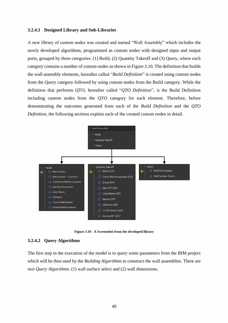
49

3.2.4.1 Designed Library and Sub-Libraries

A new library of custom nodes was created and named “Wall Assembly” which includes the

newly developed algorithms, programmed as custom nodes with designed input and output

ports, grouped by three categories: (1) Build, (2) Quantity Takeoff and (3) Query, where each

category contains a number of custom nodes as shown in Figure 3.10. The definition that builds

the wall-assembly elements, hereafter called “Build Definition” is created using custom nodes

from the Query category followed by using custom nodes from the Build category. While the

definition that performs QTO, hereafter called “QTO Definition”, is the Build Definition

including custom nodes from the QTO category for each element. Therefore, before

demonstrating the outcomes generated from each of the Build Definition and the QTO

Definition, the following sections explain each of the created custom nodes in detail.

Figure 3.10 - A Screenshot from the developed library

3.2.4.2 Query Algorithms

The first step in the execution of the model is to query some parameters from the BIM project

which will be then used by the Building Algorithms to construct the wall assemblies. There are

two Query Algorithms: (1) wall surface select and (2) wall dimensions.

50

3.2.4.2.1 Wall Surface Select Algorithm

The function of the Wall Surface Select algorithm is to query the exterior surfaces of each wall

element to be used in the build algorithms as base planes for placement of the assembly

elements. The geometric representation of a wall element in Revit® is simply a solid formed

by the extrusion of a poly-surface in a direction perpendicular to this surface called thickness.

A typical wall solid would have six faces/surfaces; however, wall elements with

inserts/windows/doors would have more than six surfaces, thus an automated method is needed

to select the wall surfaces that can act as base planes for the placement of the different assembly

elements.

A custom node was designed that requires on input which is the

“wall types” of the native BIM project and produces a number of

four outputs in the form of arrays: (1) wall-wall surface, (2) wall-

wall elements, (3) wall-col surfaces, and (4) wall-col elements as

shown in Figure 3.11. The outputs from this node were designed

to be four outputs instead of two since two outputs are used for

elements that can be placed on walls between two columns and the

other two outputs are used for elements in walls with L-connection.

The flow chart of the algorithm is shown in Figure 3.12.

The algorithm starts by one input which is the wall type in the BIM project. All the wall

elements under this wall type are queried as solids, imported to the Dynamo® canvas for further

manipulation and processing. A topology function is applied on all the imported solids to query

the surfaces in each. The topology function generates an array of surfaces in which each row

in the array represents a wall element and each column represents the number of surfaces. A

surface area query function is applied to generate the values of the surface areas of each surface

as shown in Equation 2. Typically, the surfaces that are required to be obtained from each wall

element is the surface with that largest area; however, each wall element will generate two

surfaces that have the same surface areas as shown in Figure 3.13. Therefore, the values are

sorted descending and then the first two columns in each row are grouped under a separate

array for further processing.

Figure 3.11 - Wall Surface Select

Custom Node

51

Start

Wall Type

Get Wall Elements

Get Surface Areas for each element

Sort Decending

Get First two items

CreatePoint on Surface at

Parameter p = (0.5,0.5)

Get Normal Vector at Point

Same Direction

Interior Surface

Exterior Surfaces

CreatePoint on Surface at

Parameter p = (0.5,0.5)

Get Normal Vector at Point

Get X Component

Get Keys Group Elements by Key

Horizontal Elements

Vertical Elements

Create Normalized Vectors in X and Y

Get Solid Get Solid

Geometry Intersect

Non-Intersecting

Elements

Intersecting Elements

Horizontal Surfaces

Vertical SurfacesSimilar

Values ?

Get Keys

Match Keys

Non-Intersecting

Surfaces

Intersecting Surfaces

End

Figure 3.12 - Flowchart for the Wall Surface Select Algorithm

𝐒𝐀 = [

𝑠𝑎11 𝑠𝑎12 ⋯ 𝑠𝑎1𝑚

𝑠𝑎21 𝑠𝑎22 ⋯ 𝑠𝑎2𝑚

⋮ ⋮ ⋱ ⋮𝑠𝑎𝑛1 𝑠𝑎𝑛2 ⋯ 𝑠𝑎𝑛𝑚

]

where n is the number of wall elements and m is the number surface per wall element

(2)

52

Figure 3.13 - That largest two surface areas are highlighted in blue, one this side and one the other side of the wall

In general, surfaces are defined by a function and two parameters “u” and “v”. Thus, the surface

domain is the range of (u,v) parameters that generate points on the surface. The domain of each

parameter is normalized, meaning the both u and v take values from 0 to 1 as shown in Figure

3.14.

Figure 3.14 - The definition of UV coordinate system when working with surfaces (dynamoprimer.com)

The next step is selecting the exterior surfaces from each of the two surfaces under each wall

element. First a point was created on each of the two surfaces at parameter (0.5,0.5).

Unfortunately, the textual representation cannot be expressed here since this is a 3D array

where each wall element has two surfaces, each surface has a point of two u,v coordinates. The

next step is to generate a normal unit vector from the placed point on each surface. One way of

sorting surfaces is to group surfaces that have a normal unit vector parallel or in the same

direction as universal unit vectors; in other words, if the normal at each surface center point is

parallel or in the same direction as the universal unit vector �⃗� = (1,0,0) then such surfaces are

grouped under the name exterior surfaces, the remainder surfaces would be grouped under

interior surfaces as shown in Figure 3.15.

53

Figure 3.15 - Highlighted surfaces are marked as exterior surfaces that are parallel or in the same direction as the

universal unit vector �⃗�

The next step is to group these exterior surfaces by horizontal and vertical direction. This was

done by again creating a point on each of these surfaces at u,v (0.5,0.5), but then querying the

values of the generate points on each surface with respect to the universal coordinate system

(x,y,z). Thus, surfaces with “x” component of equal values can be grouped as horizontal

surfaces while the remainder surfaces can be grouped as vertical surfaces. By using the key

values of the horizontal surfaces, the list of wall elements can be sorted grouped by keys, thus

producing two lists of wall elements horizontal and vertical elements.

Converting both the horizontal and vertical lists of wall elements to solids than performing a

geometric intersection between these two lists of solid generates the intersecting solids in a list

and the non-intersecting solid in the other list. In a broader view, intersecting solids represent

two wall elements forming a L-connection while non intersecting solids from wall elements

that are bound by columns from each side. Again, using the keys of the non-intersecting solids,

exterior surfaces can be sorted and grouped by keys to produce non-intersecting surfaces and

intersecting surfaces.

3.2.4.2.2 Wall Dimensions Algorithm

The function of Wall Dimensions algorithm is to query the “Length” and “Height” per wall in

the native BIM project. In Revit® the length of the wall is easily determined by querying the

“length” parameter of each wall. However, for the height, Revit® calculates the height of the

wall based on the difference between the two levels which are the wall base constraint and the

top constraint and is allocated under “unconnected height” parameter. Unfortunately, querying

the heights of walls is not straight forward process since Revit® fails to determine the walls’

54

heights for irregular profiles as shown in Figure 3.16, where the wall properties window show

that the unconnected height parameter = 3000mm while an isolated view of one of the model

walls show that the wall height is variable. Therefore, the developed Wall Dimensions

algorithm creates a walk-around to querying the maximum height each wall.

Figure 3.16 - Wall heights are not correctly calculated for irregular wall profiles

The designed custom node for the Wall Dimensions require

two input lists; one for the wall elements and one for the wall

surfaces as shown in Figure 3.17. For example, if the BIM

project contains 4 walls, then each of the lists will be composed

of a 1D array with indexed with numbers starting “[0]”. Each

item in the wall elements list correspond to an item in the wall

surfaces list given that both items have the same index shown

in Figure 3.18. The outputs from this node is the length and heights of each wall. The Wall

Dimensions algorithm flowchart is shown in Figure 3.19.

Figure 3.18 - List structure of both the wall elements and their corresponding surfaces, each represented by a vector

array

Figure 3.17 - Wall

dimensions custom node

55

Start

Wall Surfaces Wall Elements

Get Perimeter Curves

Divide Each Curve by a sequence of Cartesian Points

Get Z component of each point on

each curve

Get the maximum value of Z

components (Zmax)

Get Parameter Value by Name = unconnected

height

Get Parameter Value by Name = Length

(Per Element)

Wall Length = Length

Unconnected HeightLess than Zmax ?

Wall Height = Unconnected Height

Walls Height = Zmax

False

End

True

Figure 3.19 - Wall Dimensions Algorithm Flowchart

The algorithm starts by two input lists, one for the wall elements and another for the wall

surfaces. Querying the length is a straight forward process which is done by obtaining the

parameter value by the name “length”. For the heights, this was done on two paths and selecting

the bigger value of each path. The first path is through obtaining the parameter value by the

name “unconnected height” which works for all walls except ones with irregular profile. The

second path is using the walls surfaces by obtaining the perimeter curves of each wall surface

then dividing each curve by an arithmetic sequence of equally spaced points P ={P1, P2, ⋯,

Pn}, such that Pi are the Cartesian coordinate points on each curve with values on the x, y, and

z axes. For each curve however, the result would be a 2D matrix of points P, were each curve

would include a number of 10 points as shown in Equation 3. Thus the 2D matrix would be an

array of 4 rows and 10 columns. The next step is to get the height of each point which could be

done by obtaining the value of the z component from each point then getting the maximum

value in the 2D matrix which represents the highest point in the wall as shown in Equation 4.

56

𝐏 = [

𝑃11 𝑃12 ⋯ 𝑃1𝑚

𝑃21 𝑃22 ⋯ 𝑃2𝑚

⋮ ⋮ ⋱ ⋮𝑃𝑛1 𝑃𝑛2 ⋯ 𝑃𝑛𝑚

]

where n is the number of perimeter curves and m is the number of points per curve

(3)

𝐙𝒎𝒂𝒙 = [P 𝑛𝑚 ∈ 𝐏 | P 𝑛𝑚,𝑧 = 𝑚𝑎𝑥𝑍]

where Pnm,Z = [

𝑍11 𝑍12, ⋯ 𝑍1𝑚

𝑍21 𝑍22 ⋯ 𝑍2𝑚

⋮ ⋮ ⋱ ⋮𝑍𝑛1 𝑍𝑛2 ⋯ 𝑍𝑛𝑚

]

(4)

Thus, if the unconnected height < Zmax then we use the Zmax to be the height of the wall. The

outputs are two lists; one with lengths and the other with heights for each wall element.

3.2.4.3 Build Algorithms

The second step in the execution of the model that uses the Build Algorithms to construct wall

assemblies based on the extracted surfaces from the previous query algorithms. The definition

of the building algorithms is shown in Figure 3.20.

Figure 3.20 - Model Build Definition

57

Each query or build node is preceded by an input such as family types for each build algorithm

type, some nodes require inputs in the form of numbers such as the horizontal spacing between

the vertical rebar. Each of the build algorithms will be explained separately in the upcoming

sections highlighting the function and output of each. There are eight Build Algorithms: (1)

brick stacker, (2) brick stacker L-corners, (3) lintel beam place, (4) sill beam place, (5) vertical

reinforcement, (6) joint reinforcement, (7) wall-to-column ties and (8) Top-of-Wall Sealant

place.

3.2.4.3.1 Brick Stacker Algorithm

The function of this algorithm is to stack brick elements inside each wall element in the BIM

project; considering the different wall inserts (doors/windows/openings), running bond pattern,

the different cut lengths depending on the layout and the cut height of brick for non-modular

wall heights. This algorithm works only for walls that are bound from each side by a column.

However, for intersecting walls such as corner walls or connection walls, another algorithm

was designed for these specific walls that highlights the interlocking behavior between bricks

for corner connections. The algorithm for these walls is “Brick Stacker L-Corner” algorithm

and shall be discussed in the next section.

This algorithm first requires inputs from the query

algorithms to generate the surfaces that families will be

placed upon. Figure 3.21 shows the custom node built for

this algorithm which requires three inputs: (1) wall surfaces,

(2) wall element, and (3) brick family type; and the output

constructs the brick elements in the BIM project. This

custom node was designed with three output ports to

facilitate working with the designed QTO algorithms. Figure 3.22 shows the flowchart of the

brick stacker algorithm.

The algorithm starts by the list of wall elements and wall surfaces obtained from the previous

query node “wall surface select”. Using the “wall elements” input port, the wall dimensions

are obtained (lengths and heights) via the built-in custom query node “wall dimensions”. Using

the “wall surfaces” port, a function is applied to each surface that constructs ISO lines parallel

to the u direction, where the set of ISO lines follow a number sequence denoted by “NumSeq”

according to Equation 5 & 6.

Figure 3.21 - Brick Stacker Custom Node

58

NumSeq = { 𝑥(𝑛) , 𝑥(𝑛+1) … , 1}

Where xn is the nth term in the sequence defined by equation 6,

and that n = {z | z ∈ Z+ ∧ z ≥ 0}, such that Z+ is the set of positive integer numbers.

(5)

𝑥𝑛 = 𝑛 ∗ 𝐿𝑓

𝐻𝑤

Where Lf is the length of the brick family type and Hw is the height of the wall

(6)

Start

Wall SurfacesWall Elements

Get Wall Dimensions(Custom Node)

Wall Lengths (Lw)

Wall Heights(Hw)

Brick Family

Query Length (Lf)

Draw ISO Lines in U direction by NumSeq

NumSeq:Start = 0

Step = Lf/HwEnd = 1

Place Family by Curves

Wall-to-Col Ties Family

End

Perimeter Curves

Start Points

Z Component

Z > Hw

Top perimeter curve per wall

True

Start Point

Z Component

Intersect ISO Lines with Wall Surfaces

Split ISO Lines by Even & Odd Keys

Divide Line by PntSeq

Start = 0Step = LfEnd = Lw

Divide Line by PntSeq

Start = Lf/2Step = LfEnd = Lw

Add item {0} to the start of PntSeq

Get Points on Last Line

Z Component

Get Points on Last Line

Z Component

Z even > Z odd

Remove Last Line

True

Remove Last Line

False

Draw polycurve between each

two points

Draw polycurve between each

two points

Create List of Polycurves

Curve Start Point

Z Component

Difference – 10mm

False

Create List of Polycurves

Place Family by Curves

Change Parameter Name by Value =

Height

OR

OR

Figure 3.22 - Brick Stacker Algorithm Flowchart

59

Intersecting the array of ISO lines with surfaces, generates ISO lines on each surface but are

cut through voids as shown in Figure 3.23 and Equation 7.

𝐋 = [

𝑙11 𝑙12 ⋯ 𝑙1𝑚

𝑙21 𝑙22 ⋯ 𝑙2𝑚

⋮ ⋮ ⋱ ⋮𝑙𝑛1 𝑙𝑛2 ⋯ 𝑙𝑛𝑚

]

Where n is the number of ISO lines per m surfaces.

(7)

Figure 3.23 - ISO Lines on wall surfaces (left), intersection of ISO lines with wall surfaces (right)

The next step is splitting the array of ISO lines per surface into two sets of array, one

representing the even ISO lines and the other representing the odd ISO lines. The reason for

this splitting is to facilitate the generation of the running bond pattern, where the first course

starts with a full-length brick and the second course starts with a half-length brick then an

overlap of a half brick between courses. Splitting the ISO line array to two arrays is done by

selecting entries with even key values and then entries with odd values as shown in Equations

8 & 9.

𝐋𝒐𝒅𝒅 =

[ 𝑙11 𝑙12 ⋯ 𝑙1𝑚

𝑙31 𝑙32 ⋯ 𝑙3𝑚

𝑙51 𝑙52 ⋯ 𝑙5𝑚

⋮ ⋮ ⋱ ⋮𝑙𝑛1 𝑙𝑛2 ⋯ 𝑙𝑛𝑚]

Where n = {x | x ∈ Z+ ∧ x is odd}, such that Z+ is the set of positive integer numbers and m

is the number of surfaces.

(8)

60

𝐋𝒆𝒗𝒆𝒏 =

[ 𝑙21 𝑙22 ⋯ 𝑙1𝑚

𝑙41 𝑙42 ⋯ 𝑙3𝑚

𝑙61 𝑙62 ⋯ 𝑙5𝑚

⋮ ⋮ ⋱ ⋮𝑙𝑛1 𝑙𝑛2 ⋯ 𝑙𝑛𝑚]

(9)

Where n = {x | x ∈ Z+ ∧ x is even}, such that Z+ is the set of positive integer numbers and m is the

number of surfaces.

Each ISO line in the even list is divided by a point sequence denoted by “PntSeq” as shown in

Equation 10 & 11, where the distance between each of the points are equal. So for example, if

the length of the wall is 3000mm and Lf of the brick is 200 then PntSeq = {0,200,400,600,…,

3000}.

PntSeq = { 𝑥(𝑛) , 𝑥(𝑛+1) … , 𝐿𝑤} (10)

Where xn is the nth term in the sequence defined by equation 11, n = {z | z ∈ Z+ ∧ z ≥ 0}, such that

Z+ is the set of positive integer numbers and Lw is the length of the wall

𝑥𝑛 = 𝑛 ∗ 𝐿𝑓 (11)

Where “Lf” is the length of the brick family + 10mm the thickness of the mortar join

Similarly, for the odd list, a point sequence divides the array of ISO lines into points of equal

distances. However, this time the “PntSeq” is shown in Equation 12 &13. After constructing

this sequence the item{0} is added to the point sequence as the first item.

PntSeq = { 𝐿𝑓

2 , 𝑥(𝑛+1) … , 𝐿𝑓 }

(12)

Where xn is the nth term in the sequence defined by equation 11, n = {z | z ∈ Z+ ∧ z ≥ 0}, such that

Z+ is the set of positive integer numbers and Lw is the length of the wall

𝑥𝑛 = 𝑛 ∗ (𝐿𝑓) (13)

Where “Lf” is the length of the brick family + 10mm the thickness of the mortar join

Figure 3.24 shows the splitting of ISO lines to even and odd and dividing each array of lines

by the PntSeq as shown in the equations above.

In some cases, where wall heights are not modular (multiples of the brick thickness = 200mm),

mason may cut brick element horizontally with a height less that the actual height of the brick

to fill in the non-modular voids on top of the wall.

61

Figure 3.24 - ISO lines divided by PntSeq to be used to place bricks

Therefore, for the last ISO line in each of the even and odd arrays a start point is queried and

the “z” component is obtained which represents that height of the last line. Each of these values

are compared with the height of the wall surface as queried from the Revit® database. The wall

surfaces with ISO lines of higher elevation than the wall height are pin pointed, thus the

difference between the closest ISO line and the top most perimeter curve of the surface is

calculated and stored. For the rest of the points on all surfaces, polycurves are constructed

between each set of points which are then used as reference lines for the designed wall based

families to be placed upon. For the top most curve, the brick family is placed as well but this

time the height parameter of the bricks for this specific ISO line is altered to take the stored

value which is the difference between the highest point in the surface to the height of the wall.

The output for this point can be visualized as shown in Figure 3.25.

Figure 3.25 - The last course is constructed with a different brick height than the other courses to fit the non-modular

wall height

62

The global output from the algorithm constructs bricks within the walls in the BIM project as

shown in Figure 3.26.

Figure 3.26 - The output from the brick stacker algorithm, showing the brick stacker build definition (right)

One of the outputs generated from this algorithm is that users can detect non modular layouts

after execution of the algorithm as shown in Figure 3.27 for example, where the window is

placed in a location that will generate a lot of waste due to cutting of bricks to fit the wall as

highlighted.

Figure 3.27 - Early detection of non-modular layout issues.

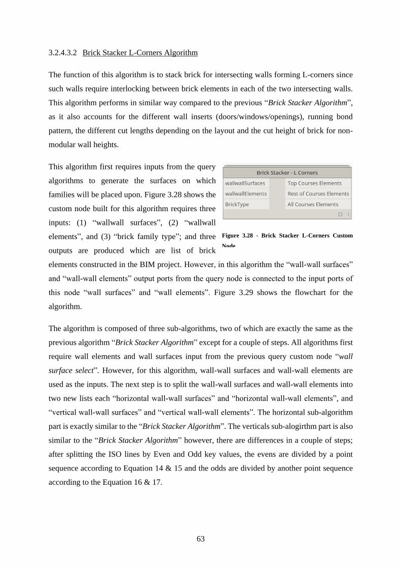
63

3.2.4.3.2 Brick Stacker L-Corners Algorithm

The function of this algorithm is to stack brick for intersecting walls forming L-corners since

such walls require interlocking between brick elements in each of the two intersecting walls.

This algorithm performs in similar way compared to the previous “Brick Stacker Algorithm”,

as it also accounts for the different wall inserts (doors/windows/openings), running bond

pattern, the different cut lengths depending on the layout and the cut height of brick for non-

modular wall heights.

This algorithm first requires inputs from the query

algorithms to generate the surfaces on which

families will be placed upon. Figure 3.28 shows the

custom node built for this algorithm requires three

inputs: (1) “wallwall surfaces”, (2) “wallwall

elements”, and (3) “brick family type”; and three

outputs are produced which are list of brick

elements constructed in the BIM project. However, in this algorithm the “wall-wall surfaces”

and “wall-wall elements” output ports from the query node is connected to the input ports of

this node “wall surfaces” and “wall elements”. Figure 3.29 shows the flowchart for the

algorithm.

The algorithm is composed of three sub-algorithms, two of which are exactly the same as the

previous algorithm “Brick Stacker Algorithm” except for a couple of steps. All algorithms first

require wall elements and wall surfaces input from the previous query custom node “wall

surface select”. However, for this algorithm, wall-wall surfaces and wall-wall elements are

used as the inputs. The next step is to split the wall-wall surfaces and wall-wall elements into

two new lists each “horizontal wall-wall surfaces” and “horizontal wall-wall elements”, and

“vertical wall-wall surfaces” and “vertical wall-wall elements”. The horizontal sub-algorithm

part is exactly similar to the “Brick Stacker Algorithm”. The verticals sub-alogirthm part is also

similar to the “Brick Stacker Algorithm” however, there are differences in a couple of steps;

after splitting the ISO lines by Even and Odd key values, the evens are divided by a point

sequence according to Equation 14 & 15 and the odds are divided by another point sequence

according to the Equation 16 & 17.

Figure 3.28 - Brick Stacker L-Corners Custom

Node

64

Figure 3.29 - Brick Stacker L-Corner Algorithm Flowchart

Hor

izon

tal

Wal

l Sur

face

s

Hor

izon

tal

Wal

l Ele

men

ts

Get

Wal

l Dim

ensi

ons

(Cus

tom

Nod

e)

Wal

l Len

gths

(L

w)

Wal

l Hei

ghts

(Hw

)

Bric

k Fa

mily

Que

ry

Leng

th (L

f)

Dra

w IS

O L

ines

in U

di

rect

ion

by N

umSe

q

Num

Seq:

Star

t = 0

Step

= L

f/H

wEn

d =

1

Plac

e Fa

mily

by

Cur

ves

Bric

k Fa

mily

Ty

pe

End

Perim

eter

Cur

ves

Star

t Poi

nts

Z Co

mpo

nent

Z >

Hw

Top

peri

met

er

curv

e pe

r w

all

True

Star

t Po

int

Z Co

mpo

nent

Inte

rsec

t ISO

Lin

es w

ith

Wal

l Sur

face

s

Split

ISO

Lin

es b

y Ev

en &

Odd

Key

s

Div

ide

Line

by

PntS

eqSt

art =

0St

ep =

Lf

End

= Lw

Even

Div

ide

Line

by

PntS

eqSt

art =

(Lf)

/2St

ep =

Lf

End

= Lw

Odd Add

item

{0} t

o th

e st

art

of P

ntSe

q

Get

Poi

nts

on

Last

Lin

eZ

Com

pone

ntG

et P

oint

s on

La

st L

ine

Z Co

mpo

nent

Z ev

en >

Z o

dd

Rem

ove

Last

Li

ne

True

Rem

ove

Last

Li

ne

Fals

e

Dra

w p

olyc

urve

be

twee

n ea

ch

two

poin

ts

Dra

w p

olyc

urve

be

twee

n ea

ch

two

poin

ts

Crea

te L

ist o

f Po

lycu

rves

Curv

e St

art

Poin

tZ

Com

pone

ntD

iffer

ence

–

10m

m

Fals

e

Crea

te L

ist o

f Po

lycu

rves

Plac

e Fa

mily

by

Cur

ves

Chan

ge P

aram

eter

N

ame

by V

alue

=

Hei

ght

OR

OR

Vert

ical

Wal

l Su

rfac

es

Vert

ical

Wal

l El

emen

ts

Get

Wal

l Dim

ensi

ons

(Cus

tom

Nod

e)

Wal

l Len

gths

(L

w)

Wal

l Hei

ghts

(Hw

)

Bric

k Fa

mily

Que

ry

Leng

th (L

f)

Dra

w IS

O L

ines

in U

di

rect

ion

by N

umSe

q

Num

Seq:

Star

t = 0

Step

= L

f/H

wEn

d =

1

Plac

e Fa

mily

by

Cur

ves

Bric

k Fa

mily

ty

pe

Perim

eter

Cur

ves

Star

t Poi

nts

Z Co

mpo

nent

Z >

Hw

Top

peri

met

er

curv

e pe

r w

all

True

Star

t Po

int

Z Co

mpo

nent

Inte

rsec

t ISO

Lin

es w

ith

Wal

l Sur

face

s

Split

ISO

Lin

es b

y Ev

en &

Odd

Key

s

Div

ide

Line

by

PntS

eqSt

art =

Lf/

2St

ep =

Lf

End

= Lw

Even

Div

ide

Line

by

PntS

eqSt

art =

0St

ep =

Lf

End

= Lw

Odd

Get

Poi

nts

on

Last

Lin

eZ

Com

pone

ntG

et P

oint

s on

La

st L

ine

Z Co

mpo

nent

Z ev

en >

Z o

dd

Rem

ove

Last

Li

ne

True

Rem

ove

Last

Li

ne

Fals

e

Dra

w p

olyc

urve

be

twee

n ea

ch

two

poin

ts

Dra

w p

olyc

urve

be

twee

n ea

ch

two

poin

ts

Crea

te L

ist o

f Po

lycu

rves

Curv

e St

art

Poin

tZ

Com

pone

ntD

iffer

ence

–

10m

m

Fals

e

Crea

te L

ist o

f Po

lycu

rves

Plac

e Fa

mily

by

Cur

ves

Chan

ge P

aram

eter

N

ame

by V

alue

=

Hei

ght

OR OR

Add

item

{0} t

o th

e st

art

of P

ntSe

q

Poin

t at

Para

met

er P

h(0

.5,0

.5)

Poin

t at

Para

met

er P

v(0

.5,0

.5)

Line

by

Ph

and

Pv

Line

D

irec

tion

Nor

mal

ize

Vect

or

X co

mpo

nent

Y co

mpo

nent

(1,1

)

(-1,

1)

(-1,

-1)

(1,-1

)

(X,Y

)

Rem

ove

Last

Po

lycu

rve

Rem

ove

Firs

t Po

lycu

rve

Rem

ove

Firs

t Po

lycu

rve

Rem

ove

Firs

t Po

lycu

rve

Rem

ove

Firs

t Po

lycu

rve

Rem

ove

Last

Po

lycu

rve

Rem

ove

Last

Po

lycu

rve

Rem

ove

Last

Po

lycu

rve

Wal

l Sur

face

sW

all E

lem

ents

Star

t

65

PntSeq = { 𝐿𝑓

2 , 𝑥(𝑛+1) … , 𝐿𝑓 }

(14)

Where xn is the nth term in the sequence defined by equation 15, n = {z | z ∈ Z+ ∧ z ≥ 0},

such that Z+ is the set of positive integer numbers and Lw is the length of the wall

𝑥𝑛 = 𝑛 ∗ 𝐿𝑓 (15)

Where “Lf” is the length of the brick family + 10mm the thickness of the mortar join

PntSeq = { 𝑥(𝑛) , 𝑥(𝑛+1) … , 𝐿𝑤} (16)

Where xn is the nth term in the sequence defined by equation 17, n = {z | z ∈ Z+ ∧ z ≥ 0}, such that

Z+ is the set of positive integer numbers and Lw is the length of the wall

𝑥𝑛 = 𝑛 ∗ 𝐿𝑓 (17)

Where “Lf” is the length of the brick family + 10mm the thickness of the mortar join

The purpose of this change is to mimic the interlocking behavior of intersecting walls forming

the L-corners. The third sub-algorithm controls the interlocking behavior between the vertical

and horizontal walls. The working principle for the interlocking sub-algorithm can be

demonstrated with the following example as shown in Figure 3.30. The flowchart for the

algorithm is shown in Figure 3.31. For example, in horizontal walls, the first brick that has any

odd key (1,3,5,…) will be removed, and in vertical walls the first brick that has any even key

(0,2,4,…) will be removed thus generating the interlocking behavior.

Figure 3.30 - The interlocking behavior between horizontal and vertical walls by removing elements at keys

66

Figure 3.31 - Interlocking sub-algorithm flowchart

The first part in the algorithm places a point on each of the horizontal and vertical wall surfaces

using a uv parameter P = (0.5,0.5) which represents the center point of each of the horizontal

and vertical surfaces. The next step is to connect each intersecting horizontal and vertical

surfaces together using the center points in each where the start point is always from the

horizontal surface and the end point is always from the vertical surfaces. The next steps are to

first determine the direction of each line, normalizing its vector components and query the (x,y)

coordinates of each vector. Depending on the quadrant of each vector the removal of the first

or last brick in the wall is determined. In general, for horizontal walls, the polycurves in any

even list remain while polycurves in any odd list an item is removed from either the start or

end of the wall. For vertical walls however, the polycurves in any odd list remain while

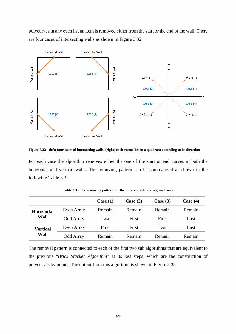
67

polycurves in any even list an item is removed either from the start or the end of the wall. There

are four cases of intersecting walls as shown in Figure 3.32.

Figure 3.32 - (left) four cases of intersecting walls, (right) each vector lies in a quadrant according to its direction

For each case the algorithm removes either the one of the start or end curves in both the

horizontal and vertical walls. The removing pattern can be summarized as shown in the

following Table 3.3.

Table 3.3 - The removing pattern for the different intersecting wall cases

Case (1) Case (2) Case (3) Case (4)

Horizontal

Wall

Even Array Remain Remain Remain Remain

Odd Array Last First First Last

Vertical

Wall

Even Array First First Last Last

Odd Array Remain Remain Remain Remain

The removal pattern is connected to each of the first two sub algorithms that are equivalent to

the previous “Brick Stacker Algorithm” at its last steps, which are the construction of

polycurves by points. The output from this algorithm is shown in Figure 3.33.

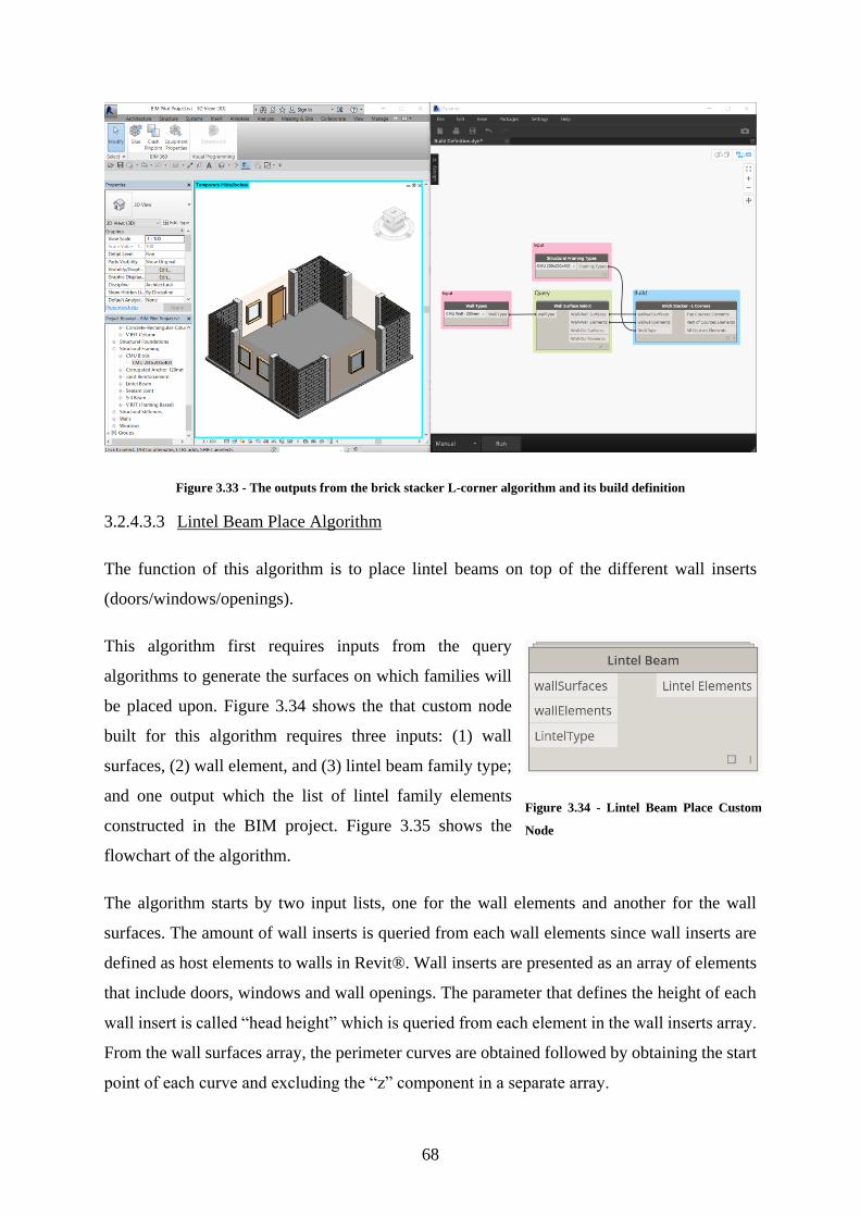
68

Figure 3.33 - The outputs from the brick stacker L-corner algorithm and its build definition

3.2.4.3.3 Lintel Beam Place Algorithm

The function of this algorithm is to place lintel beams on top of the different wall inserts

(doors/windows/openings).

This algorithm first requires inputs from the query

algorithms to generate the surfaces on which families will

be placed upon. Figure 3.34 shows the that custom node

built for this algorithm requires three inputs: (1) wall

surfaces, (2) wall element, and (3) lintel beam family type;

and one output which the list of lintel family elements

constructed in the BIM project. Figure 3.35 shows the

flowchart of the algorithm.

The algorithm starts by two input lists, one for the wall elements and another for the wall

surfaces. The amount of wall inserts is queried from each wall elements since wall inserts are

defined as host elements to walls in Revit®. Wall inserts are presented as an array of elements

that include doors, windows and wall openings. The parameter that defines the height of each

wall insert is called “head height” which is queried from each element in the wall inserts array.

From the wall surfaces array, the perimeter curves are obtained followed by obtaining the start

point of each curve and excluding the “z” component in a separate array.

Figure 3.34 - Lintel Beam Place Custom

Node

69

Start

Wall Surfaces Wall Elements

Get Perimeter Curves

Get Start Point for each Curve

Query Wall Inserts

Get Parameter Value by Name =

Head Height

Z component per point

Head Height == Z component ?

False

Filter Points

True

Create Polycurve by

Points

Place Family by Curve

Lintel Beam Family Type

End

Figure 3.35 - Lintel Beam Place Algorithm Flowchart

The next step is to obtain the set of points that have the same height (z component value) which

is equal to the head height of each insert. This is done by matching each head height with the

z component value which generates a Boolean array of True and False values. This array is

then used to filter the start point of each curve array to obtain a list of points that can be then

joined by polycurves. The final step is to place the lintel beam family type by this joined

polycurves. The output from the algorithm is shown in Figure 3.36.

Figure 3.36 - The outputs from the lintel beam place algorithm and its build definition

70

3.2.4.3.4 Sill Beam Place Algorithm

The function of this algorithm is to place sill beams below the different wall inserts

(doors/windows/openings).

The algorithm first requires inputs from the query

algorithms to generate the surfaces on which families will

be placed upon. Figure 3.37 shows the custom node built for

this algorithm requires three inputs: (1) wall surfaces, (2)

wall element, and (3) sill beam family type; and one output

is produced which the list of sill beam elements which are

constructed in the BIM project.

The working principle of this algorithm is exactly the same as that of the lintel beam place

algorithm. The only difference is that the sill height parameter is used in this algorithm

compared to the lintel beam place algorithm where the head height is used as shown in Figure

3.38.

Figure 3.38 - The difference between the head height and the sill height which is used in this algorithm

In other words, the only difference is in the querying of the sill height array and matching its

values with the z components of the start points of the wall perimeter curves and the final step

is to place the sill beam family type by these joined polycurves as shown in Figure 3.39.

Figure 3.37 - Sill Beam Place Custom Node

71

Figure 3.39 - The outputs from the sill beam place algorithm and its build definition

3.2.4.3.5 Vertical Reinforcement Algorithm

This algorithm has three functions, (1) to place the designed vertical reinforcement rebar

elements inside walls; where the vertical rebar aligns with the center line of the cores in the

CMUs used, (2) to place the minimum vertical reinforcement in case of non-load bearing walls

and (3) to place vertical dowel rebar by its embedded length inside the concrete slab and

accounting for its splice length with the vertical reinforcement in the wall.

This algorithm first requires inputs from the query

algorithms to generate the surfaces on which

families will be placed upon. Figure 3.40 shows that

the custom node built for this algorithm requires

seven inputs: (1) wall surfaces, (2) wall element, (3)

the horizontal spacing between the vertical rebar (4)

the vertical rebar family type, (5) the dowels

embedded length in the concrete slab, (6) the lap

splice length between dowels and vertical rebar and

(7) the dowel family type. The algorithm generates

three outputs (1) the vertical rebar elements, (2) the dowels element and (3) a combined list

between both. Figure 3.41 shows the flowchart of the algorithm.

Figure 3.40 - Vertical Rebar and Dowels Placement

Custom Node

72

Start

Wall Surfaces

Wall Elements

Get Wall Dimensions(Custom Node)

Wall Lengths (Lw)

Wall Heights(Hw)

Spacing

Place Point (P1) on Line at

P1 = Lc – (Lb/4)

Place Family by Curves

Get Start Point

Draw polycurve between each

two points

Draw ISO Lines in V direction by NumSeq

Start = 0Step = 0.2

End = 1

Sp == 0

Draw ISO Lines in U direction by NumSeq

Start = (105/Lw)Step = (Sp/Lw)

End = 1

True (min RFT) False (designed RFT)

Intersect Intersect

Place Point (P2) on Line atP1 = (Lb/4)

Get Line Lengths (Lc)

Construct Polycurve by P1 & P2 in

Vertical direciton

Divide Polycurve by PntSeqStart = 0

Step = 1000End = Hw

Translate in +Z By Dist = Ls

Translate in -Z By Dist = Le

Construct Polycurve in Vertical direction

Embedded Length (Le)

Splicing Length (Ls)

Place Family by Curves

VRFT Family Type

Place Family by Curves

Get Start Point

Draw polycurve between each

two points

Divide Polycurve by PntSeqStart = 0

Step = 1000End = Hw

Translate in +Z By Dist = Ls

Translate in -Z By Dist = Le

Construct Polycurve in Vertical direction

Place Family by Curves

Dowel Family Type

End

Figure 3.41- Vertical Rebar and Dowels Placement Algorithm Flowchart

The algorithm starts by two input lists, one for the wall elements and another for the wall

surfaces. For each wall in the wall element list, the wall length (Lw) and the wall height (hw)

are obtained. The user specifies the spacing required between the vertical rebar which is

typicaly every 400mm according to common practice. However, the user may specify that the

spacing is 0mm, which means that no vertical rebar is required in these walls. However,

building codes specifcy that there has to be a minimum amout of reinforcement in each CMU

73

wall, regardless of the wall’s structural behaviour (NCMA 12 4D, 2007). Therefore, a

conditional IF statement specifes which path the algorithm will proceed upon. If the spacing is

equal to zero then the minium reiforcement path will be used, and if the spacing is bigger than

zero then the designated spacing will be included in the calculation another path will be

executed.

For the minimum reinforcemnt path, ISO lines in the V direction (that are parralel to the U

direction) are constructed in accordance with a number sequence that starts with 0, ends at 1

and with a step of 0.2. Then the ISO lines are set for intersection with the wall surfaces to

account for each wall geoemetry including the location of the inserts. The next step is to

calculate the length of each ISO line after intersection and place two points on each line

dentored with P1 and P2 as shown in Equation 18 & 19.

P1 = 𝐿𝑐 − 𝐿𝐵

4

Where Lc is the length of each ISO line, LB is the length of the brick family used in this wall’s

construction.

(18)

P2 = 𝐿𝐵

4

Where LB is the length of the brick family used in the wall’s construction

(19)

Joining each of the P1 and the P2 together, generates the path (polycurve) of the vertical rebar

inside the wall. Since vertical rebar is placed inside the wall in segments of 1000mm then each

polycurve is divided by a point seqeunce denoted by PntSeq as shown in Equation 20 & 21.

PntSeq = { 𝑥(𝑛) , 𝑥(𝑛+1) … , 𝐻𝑤 } (20)

Where xn is the nth term in the sequence defined by equation 11, n = {z | z ∈ Z+ ∧ z ≥ 0}, such that

Z+ is the set of positive integer numbers and Lw is the length of the wall

𝑥𝑛 = 𝑛 ∗ 1000mm (21)

Using this point sequence, a polycurve is then constructed between each two points which

represent the reference lines for the placement of the vertical rebar family. Another sub-path

under this minimum reinforcement path is the placement of vertical dowels. The first point in

the PntSeq is used and translated with vector coordinates = (0,0,1) with a distance equal to the

lap splice (Ls) as input by the user. Moreover, the first point is translated again with vector

74

coordinated = (0,0,-1) with a distance equal to the embedded length (Le) as input by the user.

According to NCMA 12 – 4D (2007) the typical lap splice is equal to 500mm and the typical

embedded length is equal to 150mm. Vertical polycurves are constructed between the

translated points which represent the reference lines for the vertical dowels reinforcement. The

other path that uses the designed vertical reinforcement, is similar in the construction of the

vertical dowels but different in the construction of the vertical rebar across each wall itself. The

first step is drawings ISO lines in the U direction (parallel to the V direction) with a number

sequence as shown in Equations 22 & 23.

NumSeq = { 105

𝐿𝑤 , 𝑥(𝑛+1) … , 1 }

(22)

Where xn is the nth term in the sequence defined by equation 23, n = {z | z ∈ Z+ ∧ z ≥ 0}, such that

Z+ is the set of positive integer numbers and Lw is the length of the wall

𝑥𝑛 =𝑆𝑝

𝐿𝑤

Where Sp is the spacing and Lw is the length of the wall

(23)

Then intersecting the ISO lines with their surfaces and dividing each ISO by a point sequence

that start with 0 ends with the height of the wall and with a step of 1000mm which represent

the segments for the vertical rebar. Using this point sequence, a polycurve is then constructed

between each two points which represent the reference lines for the placement of the vertical

rebar family. The output from the algorithm is shown in Figure 3.42.

Figure 3.42 - The outputs from the vertical reinforcement place algorithm and its build definition

75

3.2.4.3.6 Joint Reinforcement Algorithm

The function of this algorithm is to place joint reinforcement within mortar joints between brick

elements.

This algorithm first requires inputs from the query algorithms

to generate the surfaces on which joint reinforcement families

will be placed upon. Figure 3.43 shows the custom node built

for this algorithm which requires four inputs: (1) wall

surfaces, (2) wall element, (3) joint reinforcement family

type, and (4) the placement every number of course. The

output produced which the list of the joint reinforcement

elements which are constructed in the BIM project. Figure

3.44 shows the flowchart for this algorithm.

Start

Wall Surfaces Wall ElementsCourse Count

(CC)

Draw ISO Lines in U direction by NumSeq

NumSeq:Start = 0

Step = (200*CC / Hw)End = 1

Get Wall Dimensions(Custom Node)

Wall Lengths (Lw)

Wall Heights(Hw)

Divide Each ISO Line by PntSeq

PntSeq:Start = 0

Step = 1000End = Lw

Draw PolyCurves by Points

Place Family by Curves

Joint RFT Family Type

End

Intersect Each ISO Line with Surface

Figure 3.44 - Joint Reinforcement Algorithm Flowchart

Figure 3.43 - Joint Reinforcement Place

Custom Node

76

The algorithm starts by two input lists, one for the wall elements and another for the wall

surfaces. Using the query node wall dimensions, an array of each wall height (Hw) and wall

lengths (Lw) are obtained. The next step is dividing wall surfaces into a grid of lines which is

done by constructing a sequence of ISO lines on the V axis that are parallel to the U axis of the

surface. This number sequence starts at 0 and ends at 1, where the step in the sequence is

defined by Equations 24 & 25. For example, if Hw = 3000mm, Hb = 200mm and cc=1 then the

number sequence would be = {0, 0.066, 0.133, …, 1}.

NumSeq = {𝑥(𝑛) , 𝑥(𝑛+1) … , 1} (24)

Where xn is the nth term in the sequence defined by equation 25, n = {z | z ∈ Z+ ∧ z ≥ 0}, such that

Z+ is the set of positive integer numbers and Lw is the length of the wall

𝑥𝑛 = 𝑛 ∗ 𝐻𝑏 ∗ 𝑐𝑐

𝐻𝑤 (25)

Where Hb is the height of a brick, cc is the course count and Hw is the height of the wall

The next step is intersecting the array of ISO lines with each surface, the result of the

intersection the same array of ISO lines but are cut at the voids in each surface, where voids

represent the wall inserts. To construct the curves that will be used for placing the joint

reinforcement family, each ISO line from the previous step is divided by a sequence of equally

spaced points where the distance between each two points represent the cut length of the family

to be placed on this line. the sequence of equally spaced points is defined as shown in Equation

26. For example, if the Lw = 3000mm then PntSeq = {0, 1000, 2000, 3000}

PntSeq = { 𝑥(𝑛) , 𝑥(𝑛+1) … , 𝐿𝑤} (26)

Where xn is the nth term in the sequence defined by equation 27, n = {z | z ∈ Z+ ∧ z ≥ 0}, such that

Z+ is the set of positive integer numbers and Lw is the length of the wall

xn = n * 1000 (27)

The final step is constructing polycurves between the array of points defined by the sequence

in Equation 26, then placing the joint reinforcement family type on the constructed polycurve.

The output from the algorithm is construction of the joint reinforcement within the walls in the

BIM project as shown in Figure 3.45.

77

Figure 3.45 - The outputs from the joint reinforcement place algorithm and its build definition

3.2.4.3.7 Wall-to-Column Ties Algorithm

The function of this algorithm is to place wall-to-column ties on the edges of walls either at

every course or at every other course in a staggered way along both sides of a wall.

This algorithm first requires inputs from the query

algorithms to generate the surfaces on which the wall-to-

column families will be placed upon. Figure 3.46 shows the

custom node built for this algorithm which requires four

inputs: (1) wall surfaces, (2) wall element, (3) Wall-to-

Columns family type, and (4) the placement every number

of course. The output produced which the list of the wall-

to-column tie elements which are constructed in the BIM

project. Figure 3.47 shows the flowchart of the algorithm.

The algorithm starts by two input lists, one for the wall elements and another for the wall

surfaces. Using the query node wall dimensions, an array of each wall height (Hw) and wall

lengths (Lw) are obtained.

Figure 3.46 - Wall-to-Column Ties

Custom Node

78

Start

Wall SurfacesWall Elements

Get Wall Dimensions(Custom Node)

Wall Lengths (Lw)

Wall Heights(Hw)

Wall-to-Col Tie Family

Query Length (Lf)

Draw ISO Lines in U direction by NumSeq

NumSeq:Start = 0

Step = Thb/HwEnd = 1

Get Start PointPoint at Distance

on Curve = LfPoint at Distance on

Curve = (Lw – Lf)Get End Point

Draw PolyCurves between Points

Draw PolyCurves between Points

Course Count (CC)

CC == 1CC == 1Remove Items with

even keysRemove Items with

odd keysFalse False

Create List of Polycurves

TrueTrue

Place Family by Curves

Wall-to-Col Ties Family

End

Brick Family

Figure 3.47 - Wall-to-Column Ties Place Algorithm Flowchart

The next step is dividing wall surfaces into a grid of lines which is done by constructing a

sequence of ISO lines on the v axis that are parallel to the u axis of the surface. This number

sequence starts at 0 and ends at 1, where the step in the sequence is defined by Equation 27.

For example, if Hw = 3000mm and Hb = 200mm then the number sequence would be = {0,

0.066, 0.133, …, 1}.

NumSeq = { 𝑥(𝑛) , 𝑥(𝑛+1) … , 1} (27)

Where xn is the nth term in the sequence defined by equation 28, n = {z | z ∈ Z+ ∧ z ≥ 0}, such that

Z+ is the set of positive integer numbers and Lw is the length of the wall

𝑥𝑛 = 𝑛 ∗ 𝐻𝑏

𝐻𝑤 (28)

Where Hw is the Height of the wall and Hb is the height of the bricks used

79

The next step is to generate a list of curves on both boundaries of the wall where these curves

will act as the placement curves for the wall-to-column ties families. Following the

construction of the ISO lines on each surface, a path for each wall boundary is generated. On

path requires the generation of the start point for each ISO line then create another point on

each ISO line at a distance equal to the length of the tie family, denoted by (Lf); then joining

both points by a polycurve to generate a line segment between both points. The other path is

the opposite wall boundary where the end point of each ISO lines is created as well as another

point which is as a distance equal to the length of the wall minus the length of the family,

denoted by (Lw – Lf); then joining both points by a polycurve to generate a line segment

between both points. The next step is performing a test, if the course count (denoted by “cc”)

is equal to one, which means that ties are required to be placed at every course in the wall, then

the previously constructed line segments from each path are placed in a single array and are

used as the curves to place the wall-to-column families in the BIM project. If the course count

is 2 (which is a typical number) then ties have to be staggered in way which is done by

removing entries with odd indices from one path and entries with even indices from the other

path, then creating a list of the remaining segments to be used as basis for the placement of the

wall-to-column ties family. The output from the algorithm is construction of the wall-to-

column ties within the walls in the BIM project as shown in Figure 3.48.

Figure 3.48 -The outputs from the Wall-to-Column place algorithm and its build definition.

80

3.2.4.3.8 Top-of-Wall Sealant Place Algorithm

The function of Top-of-Wall Sealant algorithm is to place the sealant on top of walls.

This algorithm first requires inputs from the query

algorithms to generate the surfaces on which families will

be placed upon. The custom node built for this function

requires three inputs: (1) wall surfaces, (2) wall element,

and (3) sealant family type; and one output is produced

which is the construction of the sealant family type in the

BIM project as shown in Figure 3.49. The flowchart for the

algorithm is shown in Figure 3.50.

Start

End

Wall Surfaces Wall Elements

Get Height (Wall Dimensions

Custom Node)

Get Perimeter Curves from Each Surface

Get Start Point for Each Curve

Get Z Component

Height == Z ?False

List Points with Height == Z

True

Create Polycurves

through list of points

Place Family using Curves

TOW Sealant Family

Figure 3.50 - Top-of-Wall Sealant Algorithm Flowchart

The algorithm starts by two input lists, one for the wall elements and another for the wall

surfaces. Querying the wall height is done from the wall elements using the wall surfaces to

obtain the perimeter curves of each wall surface then querying the start point per curve P ={P1,

P2, ⋯, Pn}, such that Pi are the Cartesian coordinate start point on each curve with values on

Figure 3.49 - Top of Wall Sealant Custom

Node

81

the x, y, and z axes. For each curve however, the result would be an array of points P, were

each curve would include a point per curve as shown in Equation 29. The next step is obtaining

the “z” component in each point as shown in Equation 30.

𝐏 = [

𝑃11

𝑃21

⋮𝑃𝑛1

]

Where n is the number of perimeter curves and P is the start point per curve.

(29)

𝐏n,𝑧 = [

𝑍11

𝑍21

⋮𝑍𝑛1

] (30)

Following these steps is matching the “z” values with the array of the height of the walls, this

filters the array into “z” component array into the set of points with z component equal to the

height of the wall. By joining these set of point by polycurves creates the reference lines for

the placement of line-based families. The next step is placing the TOW sealant family on the

set of polycurves to construct the TOW sealant elements in the wall assembly as shown in

Figure 3.51.

Figure 3.51 - The outputs from the TOW sealant algorithm and its build definition

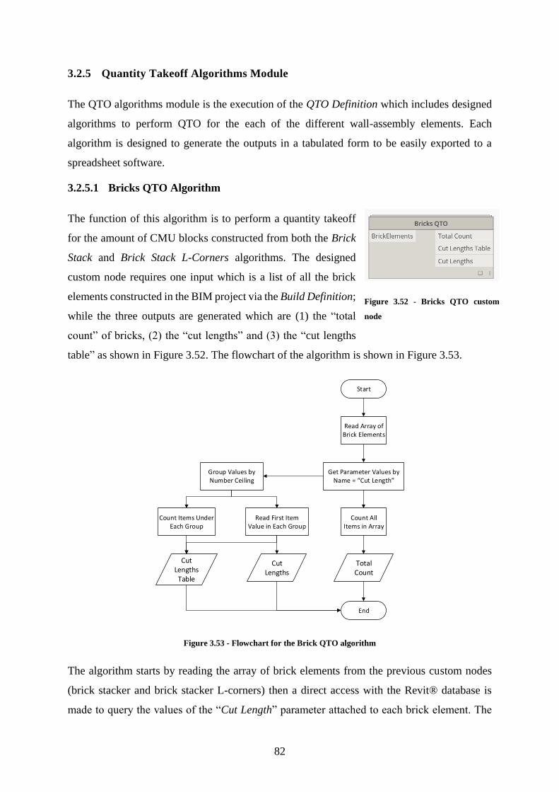
82

3.2.5 Quantity Takeoff Algorithms Module

The QTO algorithms module is the execution of the QTO Definition which includes designed

algorithms to perform QTO for the each of the different wall-assembly elements. Each

algorithm is designed to generate the outputs in a tabulated form to be easily exported to a

spreadsheet software.

3.2.5.1 Bricks QTO Algorithm

The function of this algorithm is to perform a quantity takeoff

for the amount of CMU blocks constructed from both the Brick

Stack and Brick Stack L-Corners algorithms. The designed

custom node requires one input which is a list of all the brick

elements constructed in the BIM project via the Build Definition;

while the three outputs are generated which are (1) the “total

count” of bricks, (2) the “cut lengths” and (3) the “cut lengths

table” as shown in Figure 3.52. The flowchart of the algorithm is shown in Figure 3.53.

Start

Read Array of Brick Elements

Get Parameter Values by Name = Cut Length

Group Values by Number Ceiling

Read First Item Value in Each Group

Count Items Under Each Group

Count All Items in Array

Total Count

Cut Lengths

Cut Lengths

Table

End

Figure 3.53 - Flowchart for the Brick QTO algorithm

The algorithm starts by reading the array of brick elements from the previous custom nodes

(brick stacker and brick stacker L-corners) then a direct access with the Revit® database is

made to query the values of the “Cut Length” parameter attached to each brick element. The

Figure 3.52 - Bricks QTO custom

node

83

cut length parameter represents the length of each brick element after placement inside the

model. The array of cut lengths is then grouped by number value to generate a 2D array where

each row in the array represents the number of groups and each column represents the values

under each group where all values under each group are of equal values. Therefore, the 2D

array could be minimized to be a (nx2) array where the first column contains the cut lengths

and the second column contains the countmax of each cut length as shown in Equation 31.

𝐂𝐋 = [

𝑐𝑙11 𝑐𝑙12 ⋯ 𝑐𝑙1𝑚

𝑐𝑙21 𝑐𝑙22 ⋯ 𝑐𝑙2𝑚

⋮ ⋮ ⋱ ⋮𝑐𝑙𝑛1 𝑐𝑙𝑛2 ⋯ 𝑐𝑙𝑛𝑚

] ⟹ [

𝑐𝑙11 𝑐𝑡11

𝑐𝑙21 𝑐𝑡21

⋮ ⋮𝑐𝑙𝑛1 𝑐𝑡𝑛1

]

where cl is the cut length value, ct is the count of each row, n is the number of rows and m

is the number of columns

(31)

The output could then be transposed and exported to MS Excel in the form of a table as shown

in Figure 3.54.

Figure 3.54 - The output from the Brick QTO algorithm exported in a tabular form

Another function of this algorithm is that it can test for non-modular layouts which is clearly

highlighted in the output table in the above Figure where non-modular cut lengths were found

such as cut length = 40 mm with a count of 8.

84

3.2.5.2 Mortar QTO Algorithm

The function of this algorithm is to perform a quantity

takeoff for the amount of mortar joints constructed from

Brick Stack and Brick Stack L-Corners algorithms. The

placement of mortar on CMUs does not cover the whole top

surface area of the block, instead mortar is spread around

the circumference of both face webs with a thickness

typically equal to 10mm as a common practice or as

specified in the project specifications as shown in Figure

3.56. Therefore, the designed custom node requires two

inputs which are: (1) the list of “brick elements” and the list

of “surfaces” a list of that were constructed in the BIM

project via the Build Definition; while the one output is

generated which the “total volume of mortar (m3)” as shown

in Figure 3.55. The flowchart for the algorithm is shown in

Figure 3.57.

Start

Read Array of Wall Surfaces

Get Surface Area

Get Parameter Values by Name

= Thickness

Read Array of Brick Elements

Get Parameter Values by Name =

Volume

Volume of Mortar

End

Net Planar Surface Area

Difference

Inverse

Bricks Planar Areas

Get Parameter Values by Name =

FaceWidth

Product

Figure 3.57 - Flowchart for the Mortar QTO algorithm

Figure 3.55 - Mortar QTO custom node

Figure 3.56 - The spread of mortar joints

around the circumference the face webs

only

85

The algorithm starts by two input lists, one for the wall surfaces and another for the brick

elements. Thus, the alogirthm works in two paths. The first path is querying the “surface area”

for each wall surface as shown in Equation 32. The second path is to query both the “volume”

and the “thickness” parameters for each constructed brick. Dividing the volume and thickness

parameters generates the bricks planer surface areas as per Equation 33.

𝐀𝑤𝑎𝑙𝑙𝑠 = [

𝐴𝑤1

𝐴𝑤2

⋮𝐴𝑤𝑛

]

Where, “Awn” is the surface area of wall n

(32)

𝐏𝐀𝑏𝑟𝑖𝑐𝑘𝑠 = [

𝑣1

𝑣2

⋮𝑣𝑛

] ⋅ [

𝑡ℎ1

𝑡ℎ2

⋮𝑡ℎ𝑛

]

−1

⟹ [

𝐴𝑏1

𝐴𝑏2

⋮𝐴𝑏𝑛

]

Where “PAbricks” is the planar surface area of the bricks, “vn” is the volume per brick, “thn”

is the thickness of each brick and “Abn” is the planar surface area of each brick

(33)

Thus the difference between the walls surface areas and the bricks plannar surface areas

generates the net planar surface areas as per equation 34.

𝐏𝐀𝑛𝑒𝑡 = 𝐀𝑤𝑎𝑙𝑙𝑠 − 𝐏𝐀𝑏𝑟𝑖𝑐𝑘𝑠 (34)

The volume of mortar is calculated multiplying the net planar surface areas (as per Equation

33) by two times the facewidth of each block. This results in an array of the volume of mortar

required for each brick as per Equation 35. Thus the total volume of mortar will be equal to the

summation of the values in the array as per Equation 36.

𝐕mortar = [

𝑝𝑎1

𝑝𝑎2

⋮𝑝𝑎𝑛

] ⋅ [

𝑓𝑤1

𝑓𝑤2

⋮𝑓𝑤𝑛

] ⟹ [

𝑉𝑚1

𝑉𝑚2

⋮𝑉𝑚𝑛

]

Where “pan” is new area per element, “fw” is the face width per element and “Vmn” is the

volume of mortar per element.

(35)

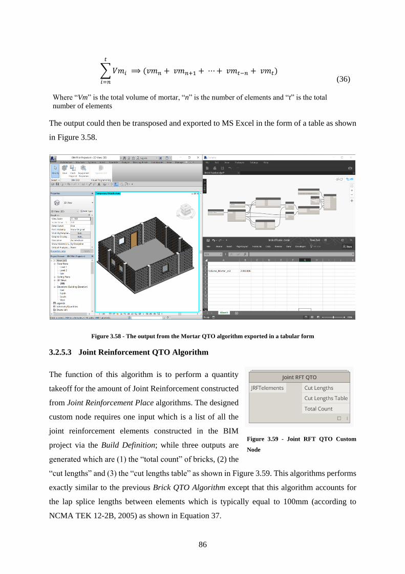
86

∑𝑉𝑚𝑖

𝑡

𝑖=𝑛

⟹ (𝑣𝑚𝑛 + 𝑣𝑚𝑛+1 + ⋯+ 𝑣𝑚𝑡−𝑛 + 𝑣𝑚𝑡)

Where “Vm” is the total volume of mortar, “n” is the number of elements and “t” is the total

number of elements

(36)

The output could then be transposed and exported to MS Excel in the form of a table as shown

in Figure 3.58.

Figure 3.58 - The output from the Mortar QTO algorithm exported in a tabular form

3.2.5.3 Joint Reinforcement QTO Algorithm

The function of this algorithm is to perform a quantity

takeoff for the amount of Joint Reinforcement constructed

from Joint Reinforcement Place algorithms. The designed

custom node requires one input which is a list of all the

joint reinforcement elements constructed in the BIM

project via the Build Definition; while three outputs are

generated which are (1) the “total count” of bricks, (2) the

“cut lengths” and (3) the “cut lengths table” as shown in Figure 3.59. This algorithms performs

exactly similar to the previous Brick QTO Algorithm except that this algorithm accounts for

the lap splice lengths between elements which is typically equal to 100mm (according to

NCMA TEK 12-2B, 2005) as shown in Equation 37.

Figure 3.59 - Joint RFT QTO Custom

Node

87

𝐂𝐋𝑡𝑜𝑡 = 𝐂𝐋 + 𝑆𝑝𝑙𝑖𝑐𝑒

Where “CLtot” is the total cut length of each joint RFT and splice is the “splice” length which

is typically 100mm long.

(37)

The output could then be transposed and exported to MS Excel in the form of a table as shown

in Figure 3.60.

Figure 3.60 - The output from the JointRFT QTO algorithm exported in a tabular form

3.2.5.4 Vertical Reinforcement QTO Algorithm

The function of this algorithm is to perform a quantity

takeoff for the amount of Vertical Reinforcement and

Vertical Dowels constructed from Vertical

Reinforcement Place algorithm. The designed custom

node requires one input which is a list of all the vertical

reinforcement elements constructed in the BIM project

via the Build Definition; while three outputs are

generated which are (1) the “cut lengths” of elements, (2) the “cut lengths” and (3) the

“itemized lengths” as shown in Figure 3.61. Since the veritcal reinforcement place algorithm

produces three outputs; (1) vertical reinforcement elements, (2) vertical dowels elements and

(3) a compiled list of both elements. Thus, this node could be placed three times depending on

Figure 3.61 - Vertical RFT QTO Custom

Node

88

the type of QTO data needed as shown in Figure 3.62. The Flowchart for this algorithm is

shown in Figure 3.63.

Figure 3.62 - Placing the Vertical RFT QTO node three times depending on the output data required

This algorithms performs exactly similar to the previous Brick QTO Algorithm as shown in

Figure 3.63,except that this algorithm accounts for two differences. The lap splice lengths

between elements which is typically equal to 200mm for the (according to NCMA TEK 12-

4D, 2007) as shown in Equation 38.

𝐂𝐋𝑡𝑜𝑡 = 𝐂𝐋 + 𝑆𝑝𝑙𝑖𝑐𝑒

Where “CLtot” is the total cut length of each joint RFT and splice is the “splice” length

which is typically 200mm long

(38)

And, (2) the values of the “Cut Length” parameter queried directly from the Revit® database

is kept itemized which produces a (nx1) 2D array, where n is the number of row (itemized cut

lengths) as shown in Equation 39.

89

𝐂𝐋 = [

𝑐𝑙1𝑐𝑙2⋮

𝑐𝑙𝑛

]

where cl is the cut length value, and n is the number of elements

(39)

Start

Read Array of Brick Elements

Get Parameter Values by Name = Cut Length

Group Values by Number Ceiling

Read First Item Value in Each Group

Count Items Under Each Group

Itemized Lengths

Cut Lengths

Cut Lengths

Table

End

Figure 3.63 - Flowchart for the Vertical RFT QTO algorithm

The output could then be transposed and exported to MS Excel in the form of as shown in

Figure 3.64.

Figure 3.64 - The output from the Vertical RFT QTO algorithm exported in a tabular form

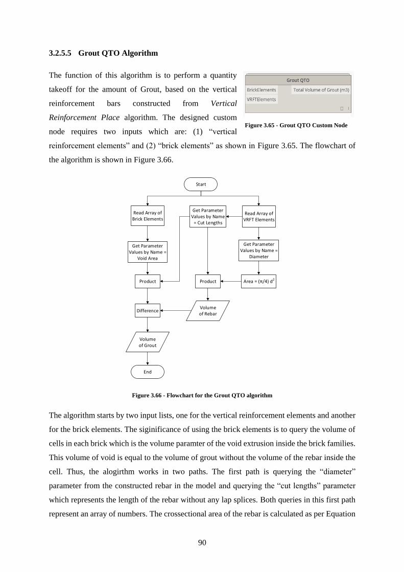
90

3.2.5.5 Grout QTO Algorithm

The function of this algorithm is to perform a quantity

takeoff for the amount of Grout, based on the vertical

reinforcement bars constructed from Vertical

Reinforcement Place algorithm. The designed custom

node requires two inputs which are: (1) “vertical

reinforcement elements” and (2) “brick elements” as shown in Figure 3.65. The flowchart of

the algorithm is shown in Figure 3.66.

Start

Read Array of Brick Elements

Get Parameter Values by Name =

Void Area

Get Parameter Values by Name

= Cut Lengths

Read Array of VRFT Elements

Get Parameter Values by Name =

Diameter

Difference

Volume of Grout

End

Product

Volume of Rebar

Product Area = (π/4) d2

Figure 3.66 - Flowchart for the Grout QTO algorithm

The algorithm starts by two input lists, one for the vertical reinforcement elements and another

for the brick elements. The siginificance of using the brick elements is to query the volume of

cells in each brick which is the volume paramter of the void extrusion inside the brick families.

This volume of void is equal to the volume of grout without the volume of the rebar inside the

cell. Thus, the alogirthm works in two paths. The first path is querying the “diameter”

parameter from the constructed rebar in the model and querying the “cut lengths” parameter

which represents the length of the rebar without any lap splices. Both queries in this first path

represent an array of numbers. The crossectional area of the rebar is calculated as per Equation

Figure 3.65 - Grout QTO Custom Node

91

38. Thus to get the volume of the rebar for each, the cut lengths are multiplied by the cross-

sectional area as per Equation 40 & 41.

𝐀𝑟𝑒𝑏𝑎𝑟 = 𝜇

4 ⋅ [

𝑑1

𝑑2

⋮𝑑𝑛

] ⋅ [

𝑑1

𝑑2

⋮𝑑𝑛

] ⟹ [

𝑎1

𝑎2

⋮𝑎𝑛

]

Where “dn” is the diameter per rebar and “an” is the cross-sectional area per rebar

(40)

𝐕rebar = [

𝑐𝑙1𝑐𝑙2⋮

𝑐𝑙𝑛

] ⋅ [

𝑎1

𝑎2

⋮𝑎𝑛

] ⟹ [

𝑉1

𝑉2

⋮𝑉𝑛

]

Where “cln” is the cut length per rebar, “an” is the area per rebar and “Vn” is the volume per

rebar.

(41)

The second path is querying the volume of the voids in the used brick type using “area”

parameter for the void extrusion. However, this number should be divided by two since each

brick family has two cells and the void area in Revit® is calculated on the basis of all the void

area per brick. Multiplying this area by the cut length of each rebar would result in the volume

of void throughout the wall which is the volume of the grout as shown in equation 42. Thus the

total volume of grout is calculated based on Equation 43.

𝐕grout = [

𝑐𝑙1𝑐𝑙2⋮

𝑐𝑙𝑛

] ⋅ [

𝑎𝑟1𝑎𝑟2⋮

𝑎𝑟𝑛

] ⟹ [

𝑉𝑔1

𝑉𝑔2

⋮𝑉𝑔𝑛

]

Where “cln” is the cut length per rebar, ar is the cross-sectional area per rebar and “Vgn” is

the volume of grout per rebar length.

(42)

∑𝑉𝑔𝑖

𝑚

𝑖=𝑛

⟹ (𝑣𝑔𝑛 + 𝑣𝑔𝑛+1 + ⋯+ 𝑣𝑔𝑚−𝑛 + 𝑣𝑔𝑚)

Where “Vg” is the volume of grout, “n” is the number of element and “m” is the total number

of elements

(43)

The output could then be transposed and exported to MS Excel in the form of a table as shown

in Figure 3.67.

92

Figure 3.67 the output from the Grout QTO algorithm exported in a tabular form

3.2.5.6 Top-of-Wall Sealant QTO Algorithm

The function of this algorithm is to perform a quantity

takeoff for the amount of Top-of-Wall Sealant constructed

from both the Top-of-Wall Sealant Place algorithm. The

designed custom node requires one input which is a list of

all the sealant elements constructed in the BIM project via

the Build Definition; while the four outputs are generated

which are (1) the “total count” of bricks, (2) the “cut

lengths” and (3) the “cut lengths table” as shown in Figure

3.68.

The Top-of-Wall Sealant QTO algorithm is exactly the same as the Brick QTO algorithm with

similar outputs as well as shown in Figure 3.69.

Figure 3.68 - Top-of-Wall Sealant QTO

Custom Node

93

Figure 3.69 - The output from the TOW Sealant QTO algorithm exported in a tabular form

3.2.5.7 Wall-to-Column Ties QTO Algorithm

The function of this algorithm is to perform a quantity

takeoff for the amount of Wall-to-Column ties

constructed from both the Wall-to-Column Ties Place

algorithm. The designed custom node requires one input

which is a list of all the sealant elements constructed in

the BIM project via the Build Definition; while only one

outputs is generated which is the “total count” of elements as shown in Figure 3.70. The

flowchart for this algorithm is shown in Figure 3.71. This algorithms performs exactly similar

to the previous Brick QTO Algorithm, except that the alogirthm only counts the number of

constructed ties as shown in figure. The output could then be exported to MS Excel in the form

of a table as shown in Figure 3.72.

Figure 3.70 - Wall-to-Column Ties QTO

Custom Node

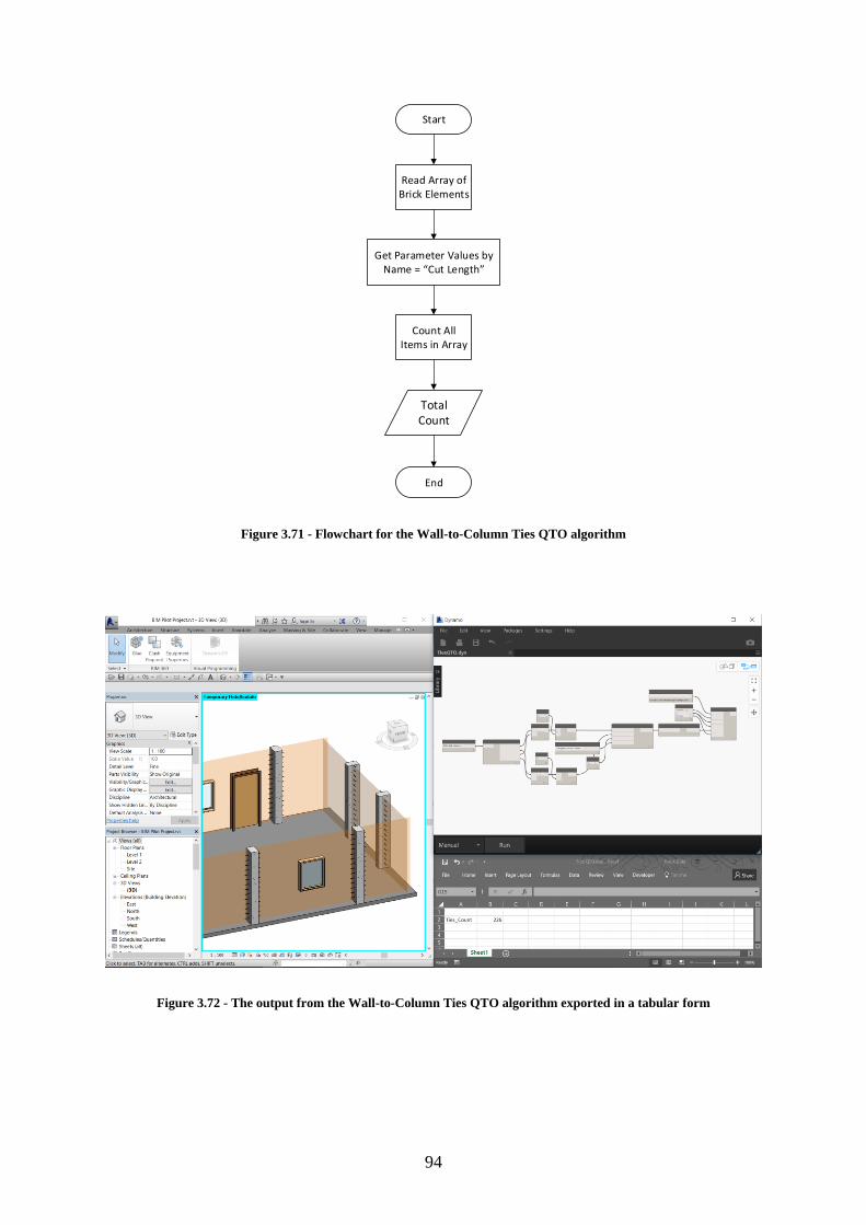
94

Start

Read Array of Brick Elements

Get Parameter Values by Name = Cut Length

Count All Items in Array

Total Count

End

Figure 3.71 - Flowchart for the Wall-to-Column Ties QTO algorithm

Figure 3.72 - The output from the Wall-to-Column Ties QTO algorithm exported in a tabular form

95

3.2.5.8 Lintel QTO Algorithm

Lintels are beams simply supported from two sides, each beam contains bottom reinforcement,

top reinforcement and shear stirrups as shown in Figure 3.73.

The function of this algorithm is to perform a

quantity takeoff for the amount of Lintel Beams

constructed from both the Lintel Beam Place

algorithm. The designed custom node requires one

input which is a list of all the Lintel elements

constructed in the BIM project via the Build

Definition; while the four outputs are generated which are (1) the “Cut Length Table” of Beams,

(2) “Stirrups Table”, (3) “Top RFT Table” and (4) “Bottom RFT Table” as shown in Figure

3.74.

Figure 3.75 shows the flowchart for the algorithm, it starts by reading the array of lintel

elements from the previous custom node (Lintel Beam Place) then a direct access with the

Revit® database is made to query the values of the “Cut Length”, “Width” and “Thickness”

parameters attached to each lintel beam element. The arrays of cut lengths, widths and

thicknesses are then grouped each by the number values to generate 2D arrays where each row

in the array represents the number of groups (Beams) and each column represents the values

(cut length/width/thickness) under each group where all values under each group are of equal

values. Therefore, each 2D array for each parameter could be minimized to be a (nx2) array

where the first column contains the cut lengths/width/thickness and the second column contains

the count of each cut length/width/thickness as shown in Equations 44, 45 & 46.

Figure 3.74 - Lintel Beam QTO Custom Node

Cut Length Jamb Jamb Width

Thickness

Stirrups

RFT Top RFT

Bottom RFT

Figure 3.73 - Typical Components of a Lintel Beam

96

Start

Read Array of Lintel

Elements

Get Parameter Values by Name = Cut Length

Group Values by Number Ceiling

Read First Item Value in Each Group

(Beam)

Count Items Under Each Group

(Beam)

Beam Cut Lengths Table

Get Parameter Values by Name = Thickness

Get Parameter Values by Name = Width

Group Values by Number Ceiling

Read First Item Value in Each Group

(Cut Length – 2* Cover / Spacing) + 1

Group Values by Number Ceiling

Read First Item Value in Each Group

2 * ((Cut Length – 2* Cover + 2*(Width –

2*Cover))

2* (Cut Length – 2 * Cover)

Read First Item Value in Each Group

Read First Item Value in Each Group

Read First Item Value in Each Group

Top RFT Table

Stirrups TableBottom RFT

Table

Start

2 * (Width + Thickness) – 4 * Cover

Figure 3.75 - Flowchart for the Lintels QTO algorithm

𝐂𝐋 = [

𝑐𝑙11 𝑐𝑙12 ⋯ 𝑐𝑙1𝑚

𝑐𝑙21 𝑐𝑙22 ⋯ 𝑐𝑙2𝑚

⋮ ⋮ ⋱ ⋮𝑐𝑙𝑛1 𝑐𝑙𝑛2 ⋯ 𝑐𝑙𝑛𝑚

] ⟹ [

𝑐𝑙11 𝑐𝑡11

𝑐𝑙21 𝑐𝑡21

⋮ ⋮𝑐𝑙𝑛1 𝑐𝑡𝑛1

]

where cl is the cut length value, ct is the count of each row, n is the number of rows and m

is the number of columns

(44)

𝐖 = [

𝑤11 𝑤12 ⋯ 𝑤1𝑚

𝑤21 𝑤22 ⋯ 𝑤2𝑚

⋮ ⋮ ⋱ ⋮𝑤𝑛1 𝑤𝑛2 ⋯ 𝑤𝑛𝑚

] ⟹ [

𝑤11 𝑐𝑡11

𝑤21 𝑐𝑡21

⋮ ⋮𝑤𝑛1 𝑐𝑡𝑛1

]

where w is the width value, ct is the count of each row, n is the number of rows and m is the

number of columns

(45)

𝐓𝐇 = [

𝑡ℎ11 𝑡ℎ12 ⋯ 𝑡ℎ1𝑚

𝑡ℎ21 𝑡ℎ22 ⋯ 𝑡ℎ2𝑚

⋮ ⋮ ⋱ ⋮𝑡ℎ𝑛1 𝑡ℎ𝑛2 ⋯ 𝑡ℎ𝑛𝑚

] ⟹ [

𝑡ℎ11 𝑐𝑡11

𝑡ℎ21 𝑐𝑡21

⋮ ⋮𝑡ℎ𝑛1 𝑐𝑡𝑛1

]

where th is the thickness value, ct is the count of each row, n is the number of rows and m is

the number of columns

(46)

97

The cut length parameter represents the width of a wall insert (door/window/opening) on which

the lintel beam is placed on its top most edge inside the model. The total length of the lintel

beam however can be calculated based on Equation 47.

𝐁𝐋 = 𝐂𝐋 + 2 ∗ 𝐉𝐋

Where BL is the total beam length array, CL is the cut lengths array and JL is the jamb

lengths array.

(47)

The following equations are then performed using each of the above parameters for each beam

element to calculate: (1) the top reinforcement table, (2) the bottom reinforcement table, (3)

the stirrups table, and (4) the lintel beams table as per the Equations 48, 49, 50, 51, 52 & 53.

Lintel Beams Table = 𝐁𝐋

where BL is the beam lengths array as in equation 8

(48)

Bottom Rft Table = 2 ∗ (𝐂𝐋 − 2Cov) + 2 ∗ (𝐓𝐇 − 2Cov)

where “CL” is the cut lengths array, “cov” is the concrete cover which is typically 30mm,

and “TH” is the thicknesses array

(49)

Top RFT Table = 2 ∗ (𝐂𝐋 − 2Cov)

Where “CL” is the cut lengths array and “Cov” is the concrete cover which is typically 30mm

(50)

Stirrups Count (ct) =𝐁𝐋 − 2Cov

Spacing+ 1

Where “BL” is the beam length array and “Spacing” is the spacing between stirrups which

is typically 200mm

(51)

Stirrups Lengths (sl) = 2 ∗ (𝐖 + 𝐓𝐇) − 4Cov

Where “W” is the widths array and “TH” is the thickness array

(52)

Stirrups Table = [

𝑠𝑙11 𝑐𝑡11

𝑠𝑙21 𝑐𝑡21

⋮ ⋮𝑠𝑙𝑛1 𝑐𝑡𝑛1

]

Where “sl” is the stirrups lengths and “ct” is the stirrups count

(53)

The output could then be transposed and exported to MS Excel in the form of a as shown in

Figure 3.76.

98

Figure 3.76 - The output from the Lintel QTO algorithm exported in a tabular form

3.2.5.9 Sill QTO Algorithm

The function of this algorithm is to perform a quantity

takeoff for the amount of Sill Beams constructed from

both the Sill Beam Place algorithm. The designed

custom node requires one input which is a list of all

the Sill elements constructed in the BIM project via

the Build Definition; while the four outputs are

generated which are (1) the “Cut Length Table” of Beams, (2) “Stirrups Table”, (3) “Top RFT

Table” and (4) “Bottom RFT Table” as shown in Figure 3.77.

The Sill QTO algorithm is exactly the same as the Lintel QTO algorithm. The only difference

is that Sill beams do not have any jamb lengths; thus the length of the sill beam will be equal

to the cut length parameter imported from Revit® database. In other words, only equation 45

in section 3.2.5.2 will be replaced with equation 54.

𝐒𝐋 = 𝐂𝐋

Where SL is the total beam length array, CL is the cut lengths array

(54)

Figure 3.77 - Sill Beam QTO Custom Node

99

4. CHAPTER 4 – CASE STUDY AND VALIDATION

This chapter presents a case study project in Cairo, Egypt that used in validation of the newly

developed wall assembly algorithms presented in this research and discussed in the previous

chapter. As-Built data from the case study project was used to compare the outcomes produced

from the execution of the model; including as-built shopdrawings, project specifications and

invoice quantity takeoff. To provide a basis for comparison, the (1) as-built shopdrawings were

compared with the geometric output of the wall-assembly model, (2) the Contractor’s material

procurement plan and the as-built quantities were compared to the outputs of the wall-assembly

QTO algorithms. A comparison between the results was then discussed.

4.1 Project Information

The presented case study is for an airfield electric Sub-station in an airport project in Egypt.

The sub-station is a single story building, with a concrete beam and slab structural system. The

building walls are made of single-wythe 200mm thick hollow core concrete masonry units

(CMUs) which are also used for the internal partitions. Autodesk® Revit® was used as the

BIM authoring tool for modeling the sub-station with up to LOD 300. BIM was mostly used

in the project for clashes detection and resolution between the different design trades.

Shopdrawings were extracted from the BIM project and were further refined with construction

details using normal 2D geometry. As of the date of this research, the blockwork activities

construction were complete and the internal and external finishes were ongoing. The data

obtained from the site Contractor included:

1. The As-built shopdrawings that were used in the actual construction of the

blockwork activities for the substation building. The as-built shopdrawings were

used as a basis of comparison to the geometric outcomes of the wall-assembly

model

2. The actual material takeoff sheets that were used by the Contractor’s procurement

team in estimating the amount of blockwork materials required in the construction

of the substation building. The calculation steps were also obtained from the

Contractor’s procurement engineers.

3. The as-built material takeoff sheets for the actual amount of procured and

constructed blockwork materials in the substation building.

100

Figure 4.1 and Figure 4.2 shows the plan view and the axonometric view for the substation

project respectively.

Figure 4.1 - Case Study Substation floor plan

Figure 4.2 - Case Study Axonometric View

The following Table 4.1 summarizes the construction information extracted from the as-built

shopdrawings, detailed drawings and project specifications. This information is then used in

101

executing the wall-assembly model, then a comparison between the as-built and the model is

conducted.

Table 4.1 - Construction information extracted from the As-Built project documents

Wall Assembly

Component Project Requirements

Masonry Units

- Hollow Core Concrete Masonry Units

- 200mm thick (nominal) 190mm thick (actual)

- Use saw cut whenever needed

- Grouted at cells with vertical RFT

Masonry

Pattern - Single wythe running bond pattern, lapping not less than 100mm

Mortar Bed

thickness - 10mm thickness

Joint

Reinforcement

- Hot-dip galvanized Steel Ladder Type

- 150mm wide - Φ5mm wires and Φ5mm cross rods

- Lap splice at 150mm

- Spacing every 2 courses (@400mm o.c.)

Vertical

Reinforcement

- Φ12mm every 800mm typical, lap splice 200mm

- Φ12mm dowel, embedded 150mm, Lap splice 500mm

Lintel Beams

- Precast/cast-insitu lintel beam

- Minimum jamb length = 200mm

- Bottom RFT = 2 Φ 12

- Top RFT = 2 Φ 12

- Stirrups = 5Φ10/200mm

Sill Beams

- Precast/cast-insitu lintel beam

- Minimum jamb length = 200mm

- Bottom RFT = 2 Φ 12

- Top RFT = 2 Φ 12

- Stirrups = 5Φ10/200mm

Wall-to-

Column

Anchors

- Galvanized steel strips

- Minimum 22 mm wide with wave length 12.7mm and amplitude of

2.5mm

- 1.9mm thick

- Extends to 200mm from the concrete face

Top-of-Wall

Compressible

Material

- 25mm thick semi-rigid polyethylene bound with two backer rods on

each edge

102

4.2 Wall-Assembly Model Application

The verification of the wall-assembly model was applied on a number of steps as shown in

Figure 4.3. The first step starts by updating the designed wall component families with the

exact parameters as the ones used in the As-built documents of the project to provide a fair

comparison between the as-built and the wall-assembly algorithm. The second step is loading

the updated families into the BIM project library so that the algorithm through accessing the

Revit® database can perform its function by using the loaded wall components. The third step

is executing the wall-assembly build definition to construction the full wall-assembly

components on the existing BIM project. Results from this step is compared to the as-built

shopdrawings to highlight the robust features of the wall-assembly algorithms. The last step is

to execute the QTO definition to calculate the quantities of wall assembly components in the

BIM project compared to the as-built quantities.

Update Family Parameters of Wall

Components

Load Updated Families to BIM

Project

Execute Wall-Assembly Build

Definition

Execute Wall-Assembly QTO

Defintion

Compare to As-Built Shopdrawings

Compare to Site QTO Method

Compare to As-Built QTO

1 2 3

4

5

6 7

Figure 4.3 - Wall Assembly Model Application Steps

4.2.1 Updating Family Parameters of Wall Components

The first step is updating the designed wall-assembly family components using information

extracted from the As-built documents of the case-study project as highlighted in Table 4.1.

Table 4.2 shows the updated family parameters with their values in each wall-assembly

component based on the information from Table 4.1.

103

Table 4.2 - Updated wall parameters as per the project requirements to be used in the case study

Wall-Assembly

Component Family Type Name Updated Parameters

Concrete Masonry Unit CMU 200x200x400

Length = 390mm

Width = 190mm

Thickness = 190mm

Joint Reinforcement J RFT D10 W150

Length = 1000mm

Width = 150mm

Diameter =10mm

Vertical Reinforcement V RFT D12 Length = 1000mm

Diameter =12mm

Lintel Beam Lintel 200x200

Base = 200mm

Height = 200mm

Jamb = 200mm

Sill Beam Sill 200x200 Base = 200mm

Height = 200mm

Wall-to-Column Anchor WtC tie 200

Thickness = 2mm

Width = 22mm

Length = 200mm

Top-of-Wall Compressible

Material ToW 25

Thickness = 25mm

Length = 1000mm

4.2.2 Load Updated Families into Project

The updated families are then loaded to the BIM case study project and under located in the

structural framing families. Loaded families means that they are easily accessible through the

Revit® database and that the Build Definition can automate the build tasks using the geometry

and parameters of each wall-assembly component.

4.2.3 Executing the Wall-Assembly Model – Build Definition

The Build Definition is first opened in Dynamo® and the case study project on Revit® is

ruining in the background. The inputs for each build-custom nodes are the family names that

each node will query its geometry and parameters from the Revit® database and construct the

wall upon. The time elapsed for the execution of the algorithm was almost 3 minutes. The

results from the execution of the build definition is shown in Figure 4.4. The build definition

constructs a full wall assembly including all its components inside of the already built wall

elements in the BIM project. By hiding the wall category from the model 3D view, the wall

assembly components could only be visible as shown in Figure 4.4.

104

Figure 4.4 - The outcomes from the execution of the Build Definition on the Case Study

4.2.4 Comparing the Wall-Assembly Model to the As-Built Shopdrawings

The next step is comparing the produced outcomes from the build definition with the as-built

shopdrawings to determine the model’s accuracy.

4.2.4.1 Concrete Blocks

Typically, concrete blocks are not drafted in shopdrawings to avoid overcrowding of drawings

and to ease out the construction process. However concrete blocks are plotted as a number of

blocks for example in the vertical direction using the modular block height and up to the clear

wall height. Figure 4.5 show the outcome generated from the CMU build algorithm. Figure 4.6

shows a comparison between a wall from the as-built shopdrawings compared to the output of

the model, where the shopdrawing highlights that this wall consists of 18 CMU blocks equally

spaced which is validated by the output of the build definition.

Figure 4.5 - Concrete blocks generation across the walls of the model upon execution of the build definition

105

Figure 4.6 - (left) as-built shopdrawing, (right) model extract for the same wall

The number of blocks or their layout are not always included on shopdrawings. However, the

wall-assembly model generates the expected layout of the blocks on each wall. Therefore, the

algorithms can be used in adjusting the locations/sizes of the wall inserts to minimize the

modular layout issues which provides insight to the planning of masonry walls construction

and thus improving the productivity of the job.

4.2.4.2 Joint Reinforcement

Joint reinforcement is typically mentioned on one of the wall section views or in the typical

detail drawings; thus the vertical spacing between each as well as the horizontal spacing could

be identified. Figure 4.7 shows a comparison between a callout detail for the locations of the

joint reinforcement on the as-built shopdrawings which mentions that the vertical spacing

between the joints reinforcement is 400mm (every other block) and the type required is ladder

type reinforcement compared to the output of the model which constructs joint reinforcement

throughout the model walls taking into account the wall inserts, lintels/sills and wall

boundaries.

Figure 4.7 - (left) as-built shopdrawing, (right) model extract for all walls

106

4.2.4.3 Vertical Reinforcement

Vertical reinforcement is expressed in wall sections to show the layout of rebar across each

wall’s length and in detail drawings to show the connection between the wall and the slab

showing the embedded length of the dowels and the lap splicing lengths in Figure 4.8.

Figure 4.8 - Typical wall section showing the layout and detail drawing

Executing the build algorithm generates vertical rebar across each wall’s length with the

specified spacing 800mm which also accounts for the wall profiles, inserts and the other

assembly elements as shown in Figure 4.9.

Figure 4.9 - Vertical rebar generation across the walls of the model upon execution of the build definition

Comparing the shopdrawing for part of a wall with the outcome from the build definition show

that also one lintel is used with the same dimension and jamb lengths, the surrounding vertical

reinforcement is also accounted for where 8 vertical bars are constructed as well compared to

the shopdrawing as shown in Figure 4.10.

107

Figure 4.10 - As-built shopdrawing, (right) model extract showing lintel beam over a door surrounded by vertical

rebar and joint reinforcement

4.2.4.4 Lintel Beams

Lintel beams are typically specified on shopdrawings in section or elevation views that has a

wall insert that requires a lintel beam. The dimensions of the lintel beams and the lengths of

the lintel jambs are also specified in different parts of the drawings. Figure 4.11 shows the

model outcome from the build algorithm where on top of any wall insert a lintel beam is

constructed that accounts for wall jambs, and the surrounding concrete blocks lengths.

Figure 4.11 - Lintel beams constructed on top of the different wall inserts and account of the surround concrete

blocks

Comparing the shopdrawing for part of a wall with the outcome from the build definition show

that also one lintel is used with the same dimension and jamb lengths, the surrounding concrete

blocks are also accounted for in terms of the different cut lengths compared to the shopdrawing

as shown in Figure 4.12.

108

Figure 4.12 - As-built shopdrawing, (right) model extract showing lintel beams over the door and window grille

surrounded by concrete blocks that where cut lengths adapt to the given space per course

4.2.4.5 Sill Beams

As Lintels, Sill beams are typically specified on shopdrawings in section or elevation views

that has a wall insert that requires a sill beam. Figure 4.13 shows the model outcome from the

build algorithm where below wall inserts, a sill beam is constructed that also accounts for the

surrounding concrete blocks lengths.

Figure 4.13 - Sill beams constructed below the different wall inserts (highlighted in blue) and account of the surround

concrete blocks

Comparing the shopdrawing for part of a wall with the outcome from the build definition show

that sill beams are constructed, surrounding concrete blocks which are also accounted for in

terms of the different cut lengths compared to the shopdrawing as shown in Figure 4.14.

109

Figure 4.14 - As-built shopdrawing vs the Wall-Assembly model outcome

4.2.4.6 Wall-to-Column Ties

Wall-to-Column ties are typically mentioned only in the typical detail drawings, where the

location is always next to a concrete column (in case of wall to concrete column ties). The

vertical spacing between the ties is based on a common practice that the ties are to be staggered

every other course. Figure 4.15 shows a comparison between a callout detail for the locations

of the wall-to-column ties on the as-built shopdrawings typical detail drawings which mentions

that the ties attach to concrete column on center of the concrete block, compared to the output

of the model which constructs the wall-to-column throughout the model walls taking into

account the staggered behavior and wall boundary profiles.

Figure 4.15 - (left) as-built shopdrawing, (right) model extract for all walls

4.2.4.7 Top-of-Wall Sealant

Top-of-Wall Sealant is typically mentioned on the typical detail drawings. The location of the

top-of-wall sealant is always between the top of the wall and the bottom of the concrete

member. Figure 4.16 shows a comparison between a callout detail for the locations of the top-

of-wall sealant on the as-built shopdrawings which mentions that its structural components,

thickness, backer rod and sealant locations compared to the output of the model which

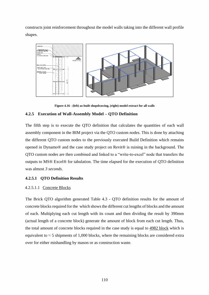
110

constructs joint reinforcement throughout the model walls taking into the different wall profile

shapes.

Figure 4.16 - (left) as-built shopdrawing, (right) model extract for all walls

4.2.5 Execution of Wall-Assembly Model – QTO Definition

The fifth step is to execute the QTO definition that calculates the quantities of each wall

assembly component in the BIM project via the QTO custom nodes. This is done by attaching

the different QTO custom nodes to the previously executed Build Definition which remains

opened in Dynamo® and the case study project on Revit® is ruining in the background. The

QTO custom nodes are then combined and linked to a “write-to-excel” node that transfers the

outputs to MS® Excel® for tabulation. The time elapsed for the execution of QTO definition

was almost 3 seconds.

4.2.5.1 QTO Definition Results

4.2.5.1.1 Concrete Blocks

The Brick QTO algorithm generated Table 4.3 - QTO definition results for the amount of

concrete blocks required for the which shows the different cut lengths of blocks and the amount

of each. Multiplying each cut length with its count and then dividing the result by 390mm

(actual length of a concrete block) generate the amount of block from each cut length. Thus,

the total amount of concrete blocks required in the case study is equal to 4982 block which is

equivalent to ≈ 5 shipments of 1,000 blocks, where the remaining blocks are considered extra

over for either mishandling by mason or as construction waste.

111

Table 4.3 - QTO definition results for the amount of concrete blocks required for the building case study

Family Type Cut Length (mm) Count Equivalent to no. of blocks

CMU Block CMU 200x200x400 40 114 11.69231

CMU Block CMU 200x200x400 90 153 35.30769

CMU Block CMU 200x200x400 140 110 39.48718

CMU Block CMU 200x200x400 190 446 217.2821

CMU Block CMU 200x200x400 240 72 44.30769

CMU Block CMU 200x200x400 270 64 44.30769

CMU Block CMU 200x200x400 290 113 84.02564

CMU Block CMU 200x200x400 340 40 34.87179

CMU Block CMU 200x200x400 390 4470 4470

Total amount of blocks 4981.282

The table above shows that there are different cut lengths other than the full block and half

block cuts that were generated from the given design of the sub-station building. Thus the QTO

algorithm provides a good indication for designers to review the modular layout issues of the

building before concluding the design. For contractors, this provides a good indication for the

expected amount of waste generated from the construction of concrete blocks as well as

assistance in the material procurement and the planning for walls construction.

4.2.5.1.2 Vertical Reinforcement

The Vertical reinforcement QTO algorithm generated Table 4.4, which shows the different cut

lengths and the amounts of each. The weight of the vertical reinforcement is calculated via

multiplying the total rebar lengths by the weight per meter for each rebar diameter. For this

case D12 is used which has 0.889 kg/m’. Multiplying the lengths by the count and the weight

per meter generates the total weight of reinforcement required which is equal to ≈ 696 kg out

of which 78 kg is for the vertical dowels.

Table 4.4 - QTO definition results for the amount of vertical reinforcement required for the case study building

Family Type Cut Length (mm) Count Kg

Vertical Reinforcement V RFT D12 1200 488 520.60

Vertical Reinforcement V RFT D12 1175 2 2.09

Vertical Reinforcement V RFT D12 1000 1 0.89

112

Vertical Reinforcement V RFT D12 800 119 84.63

Vertical Reinforcement V RFT D12 750 3 2.00

Vertical Reinforcement V RFT D12 734 4 2.61

Vertical Reinforcement V RFT D12 666 4 2.37

Vertical Reinforcement V RFT D12 650 120 78

Vertical Reinforcement V RFT D12 600 11 5.87

Vertical Reinforcement V RFT D12 575 3 1.53

Vertical Reinforcement V RFT D12 400 9 3.20

Total Kg required 695.13

4.2.5.1.3 Joint Reinforcement

The Joint reinforcement QTO algorithm generated Table 4.5 - QTO definition results for the

amount of joint reinforcement required for the case study building, which shows the different

cut lengths and the amounts of each. Multiplying each cut length with its count and then

dividing the result by 1000mm generate the metered amount of joint reinforcement. Thus, the

total amount of joint reinforcement required in the case study is equal to 1112 m which is

equivalent to ≈ 371 pellets (3m length each).

Table 4.5 - QTO definition results for the amount of joint reinforcement required for the case study building

Family Type Cut Length (mm) Count No. of pallets (1m each)

Joint Reinforcement J RFT D10 W150 200 22 4.4

Joint Reinforcement J RFT D10 W150 300 42 12.6

Joint Reinforcement J RFT D10 W150 320 9 2.88

Joint Reinforcement J RFT D10 W150 325 6 1.95

Joint Reinforcement J RFT D10 W150 375 8 3

Joint Reinforcement J RFT D10 W150 400 8 3.2

Joint Reinforcement J RFT D10 W150 450 17 7.65

Joint Reinforcement J RFT D10 W150 525 20 10.5

Joint Reinforcement J RFT D10 W150 550 23 12.65

Joint Reinforcement J RFT D10 W150 575 15 8.625

Joint Reinforcement J RFT D10 W150 750 14 10.5

113

Joint Reinforcement J RFT D10 W150 775 12 9.3

Joint Reinforcement J RFT D10 W150 800 18 14.4

Joint Reinforcement J RFT D10 W150 1000 72 72

Joint Reinforcement J RFT D10 W150 1100 853 938.3

Total no. of pallets (1m each) 1111.955

4.2.5.1.4 Lintel Beams

The Lintel beams QTO algorithm generated a number of tables; for the volume of concrete in

a lintel beam, the weight of stirrups and the weight of the beam reinforcement as shown in the

following tables. The volume of concrete for the lintel beams is calculated by multiplying the

cut lengths of each beam by its count by its other dimensions. Thus, the volume of concrete

required for the case study is equal to 1.95m3 as shown in Table 4.6.

Table 4.6 - QTO definition results for the volume of Lintel beams in the case study building

Family Type Beam Lengths (mm) Count Volume

Lintel Beam Lintel 200x200 5000 1 0.1805

Lintel Beam Lintel 200x200 4700 1 0.16967

Lintel Beam Lintel 200x200 3400 2 0.24548

Lintel Beam Lintel 200x200 2900 3 0.31407

Lintel Beam Lintel 200x200 2700 5 0.48735

Lintel Beam Lintel 200x200 2400 3 0.25992

Lintel Beam Lintel 200x200 1450 3 0.157035

Lintel Beam Lintel 200x200 1400 2 0.10108

Lintel Beam Lintel 200x200 1000 1 0.0361

Total Volume (m3) 1.951205

The total weight of the stirrups is calculated by multiplying the length by the count by the

weight per meter (for D10 = 0.617 kg/m). Thus, the total weight of D10 required for the stirrups

is equal to ≈ 117 KG as shown in Table 4.7.

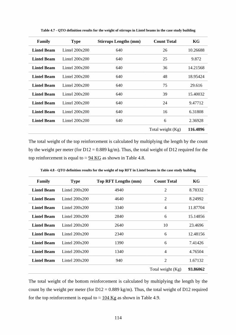
114

Table 4.7 - QTO definition results for the weight of stirrups in Lintel beams in the case study building

Family Type Stirrups Lengths (mm) Count Total KG

Lintel Beam Lintel 200x200 640 26 10.26688

Lintel Beam Lintel 200x200 640 25 9.872

Lintel Beam Lintel 200x200 640 36 14.21568

Lintel Beam Lintel 200x200 640 48 18.95424

Lintel Beam Lintel 200x200 640 75 29.616

Lintel Beam Lintel 200x200 640 39 15.40032

Lintel Beam Lintel 200x200 640 24 9.47712

Lintel Beam Lintel 200x200 640 16 6.31808

Lintel Beam Lintel 200x200 640 6 2.36928

Total weight (Kg) 116.4896

The total weight of the top reinforcement is calculated by multiplying the length by the count

by the weight per meter (for D12 = 0.889 kg/m). Thus, the total weight of D12 required for the

top reinforcement is equal to ≈ 94 KG as shown in Table 4.8.

Table 4.8 - QTO definition results for the weight of top RFT in Lintel beams in the case study building

Family Type Top RFT Lengths (mm) Count Total KG

Lintel Beam Lintel 200x200 4940 2 8.78332

Lintel Beam Lintel 200x200 4640 2 8.24992

Lintel Beam Lintel 200x200 3340 4 11.87704

Lintel Beam Lintel 200x200 2840 6 15.14856

Lintel Beam Lintel 200x200 2640 10 23.4696

Lintel Beam Lintel 200x200 2340 6 12.48156

Lintel Beam Lintel 200x200 1390 6 7.41426

Lintel Beam Lintel 200x200 1340 4 4.76504

Lintel Beam Lintel 200x200 940 2 1.67132

Total weight (Kg) 93.86062

The total weight of the bottom reinforcement is calculated by multiplying the length by the

count by the weight per meter (for D12 = 0.889 kg/m). Thus, the total weight of D12 required

for the top reinforcement is equal to ≈ 104 Kg as shown in Table 4.9.

115

Table 4.9 - QTO definition results for the weight of bottom RFT in Lintel beams in the case study building

Family Type Bottom RFT Lengths (mm) Count Total KG

Lintel Beam Lintel 200x200 5200 2 9.2456

Lintel Beam Lintel 200x200 4900 2 8.7122

Lintel Beam Lintel 200x200 3600 4 12.8016

Lintel Beam Lintel 200x200 3100 6 16.5354

Lintel Beam Lintel 200x200 2900 10 25.781

Lintel Beam Lintel 200x200 2600 6 13.8684

Lintel Beam Lintel 200x200 1650 6 8.8011

Lintel Beam Lintel 200x200 1600 4 5.6896

Lintel Beam Lintel 200x200 1200 2 2.1336

Total weight (Kg) 103.5685

4.2.5.1.5 Sill Beams

The Sill beams QTO algorithm generated a number of tables; for the volume of concrete in a

sill beam, the weight of stirrups and the weight of the beam reinforcement as shown in the

following tables. The volume of concrete for the sill beams is calculated by multiplying the cut

lengths of each beam by its count by its other dimensions. Thus, the volume of concrete

required for the case study is equal to 0.6 m3.

Table 4.10 - QTO definition results for the volume of sill beams in the case study building

Family Type Beam Lengths (mm) Count Volume (m3)

Sill Beam Sill 200x200 4300 1 0.15523

Sill Beam Sill 200x200 3000 2 0.2166

Sill Beam Sill 200x200 2000 3 0.2166

Sill Beam Sill 200x200 600 1 0.02166

0.61009

The total weight of the stirrups is calculated by multiplying the length by the count by the

weight per meter (for D10 = 0.617 kg/m). Thus, the total weight of D10 required for the stirrups

is equal to ≈ 34 KG as shown in Table 4.11.

116

Table 4.11 - QTO definition results for the weight of stirrups in sill beams in the case study building

Family Type Stirrups Lengths Count Total

Sill Beam Sill 200x200 640 22 8.68736

Sill Beam Sill 200x200 640 30 11.8464

Sill Beam Sill 200x200 640 30 11.8464

Sill Beam Sill 200x200 640 3 1.18464

Total weight (Kg) 33.5648

The total weight of the top reinforcement is calculated by multiplying the length by the count

by the weight per meter (for D12 = 0.889 kg/m). Thus, the total weight of D12 required for the

top reinforcement is equal to ≈ 30 KG as shown in Table 4.12.

Table 4.12 - QTO definition results for the weight of the top reinforcement in sill beams in the case study building

Family Type Top RFT Lengths Count Total

Sill Beam Sill 200x200 4240 2 7.53872

Sill Beam Sill 200x200 2940 4 10.45464

Sill Beam Sill 200x200 1940 6 10.34796

Sill Beam Sill 200x200 540 2 0.96012

Total weight (Kg) 29.30144

The total weight of the bottom reinforcement is calculated by multiplying the length by the

count by the weight per meter (for D12 = 0.889 kg/m). Thus, the total weight of D12 required

for the top reinforcement is equal to ≈ 33 Kg as shown in Table 4.13.

Table 4.13 - QTO definition results for the weight of the bottom reinforcement in sill beams in the case study building

Family Type Bottom RFT Lengths Count Total

Sill Beam Sill 200x200 4500 2 8.001

Sill Beam Sill 200x200 3200 4 11.3792

Sill Beam Sill 200x200 2200 6 11.7348

Sill Beam Sill 200x200 800 2 1.4224

Total weight (Kg) 32.5374

117

4.2.5.1.6 Wall-to-Column Ties

The wall-to-column ties QTO algorithm generated table which includes the lengths of the wall

to column ties used and their count. Thus, the total number of corrugated wall to column ties

required for the case study is equal to 530 piece.

4.2.5.1.7 Grout

The grout QTO algorithm generated the total volume required for the case study which is equal

to 9.58m3.

4.2.5.1.8 Mortar

The Mortar QTO algorithm generated the total volume required for the case study which is

equal to 4.26m3.

4.2.5.1.9 Top-of-Wall Sealant

The top-of-wall sealant QTO algorithm generated the total length required for the case study

which is equal to ≈ 116 m of compressible material of thickness = 25mm, surrounded by two

backer rods from two sides,

4.2.6 The site QTO method

The site QTO method is used to estimate the quantities of material required for the construction

of walls and is calculated with a set of assumptions based on the common construction

practices. The calculation steps were provided by the Contractor’s procurement team. A sample

wall from the building under consideration is used, where the wall profile is a square taking

length and height values equal to 3x3m, 4x4m, 5x5m, etc. depending on the average lengths

and heights of the walls in the building under consideration. The sample wall should also

include a door and a windows from the types already used in the building. Each component in

the wall-assembly is counted/calculated then divided by the net surface area of the wall to

generate a “value” per square meter for each assembly component. By multiplying each value

by the actual wall surface areas in the building, would roughly estimate the amount of material

required from each assembly component to construct this building. The values calculated from

this estimation exercise were the ones used in the Contractor’s procurement plan in terms of

as-planned quantities for the blockwork material procurement process.

118

For this case study, a sample wall was considered as shown in Figure 4.17. The wall contains

one door and one window with similar types as the ones used in the case study. The sample

wall dimensions have a length = 5m and height = 5m, the window dimensions are 1m x 2m

and the door dimensions are 2.3m by 2.6m, where the net area = 25m2 and the net area = 17m2.

While the As-Built area of the walls is equal to 430m2 (as extracted from one of the contractor’s

invoices).

Figure 4.17 - Sample wall for wall components quantity estimation

The following sections summarize the results from performing manual QTO on the sample

wall, calculating the value/m2 for each assembly component and then multiplying this value/m2

by the as-built area to estimate the total required material from each assembly component for

the case study.

4.2.6.1.1 Concrete Blocks

The value of the concrete blocks is calculated via dividing the total blocks required (as shown

in Table 4.14) by the net area of the wall which will be equal to 194.3/17 ≈ 11.43 CMU/m2.

Thus, the total amount of concrete blocks required in the case study is equal to 430 * 11.43 =

4914 block which is equivalent to ≈ 5 shipments of 1,000 blocks each, where the remaining

amount of block (86 block) are used as backup in case of mishandling of blocks by workers

during construction or are stored for generic uses.

2600 mm

5000 mm

1000 mm

5000 mm

2300 mm

2000 mm

119

Table 4.14 - Manual QTO for the amount of concrete blocks in the sample wall

Cut Length (mm) Count Volume (m³) No. of Blocks

90 7 0.02 1.6

190 40 0.20 19.5

290 7 0.05 5.2

390 168 1.33 168.0

Total number of blocks required 194.3

4.2.6.1.2 Vertical Reinforcement

The weight of the vertical reinforcement is calculated via multiplying the total rebar lengths by

the weight per meter for each rebar diameter. For this case D12 is used which has 0.889 kg/m’.

The total weight of vertical reinforcement required for the sample wall is equal to 22.81 kg (as

shown in table), dividing 22.81/17 ≈ 1.34 kg/m2. Thus the total amount of reinforcement

required in the case study is equal to 430 * 1.34 = 576 kg rebar of D12.

Table 4.15 Manual QTO for the amount of vertical rebar in the sample wall

Cut Length (mm) Count Kg

400 3 1.09347

600 3 1.62687

650 4 2.3114

1000 20 17.78

Total Kg required 22.81174

4.2.6.1.3 Joint Reinforcement

The value of the joint reinforcement is calculated via dividing the total length required (as

shown in Table 4.16) by the net area of the wall which will be equal to 40.4/17 ≈ 2.38 m /m2.

Thus, the total amount of joint reinforcement required in the case study is equal to 430 * 2.38

= 1023.4 m which is equivalent to ≈ 342 pellets of ladder type reinforcement (3m length each).

Table 4.16 - Manual QTO for the amount of horizontal reinforcement in the sample wall

Cut Length (mm) Count No. of pallets (1m each)

300 6 1.8

400 8 3.2

120

600 2 1.2

1000 36 36

Total no. of pallets (1m each) 40.4

4.2.6.1.4 Lintel Beams

The value of lintel beams is calculated by dividing the volume of lintels (as per Table 4.17) by

the net area of the wall which will be equal to 0.18/17 = 0.01 m3 / m2. Thus, the total amount

volume of lintels required in the case study is equal to 430 * 0.01 = 4.3 m3

Table 4.17 - Manual QTO for the volume of lintel beams in the sample wall

Length (mm) Count Volume (m3)

2400 1 0.087

2700 1 0.097

Total Volume 0.184

The amount of stirrups and reinforcement is calculated per volume of concrete for a lintel beam.

The total weight of stirrups per m3 of lintel beam (as shown in Table 4.18) is equal to 10.26/17

= 0.6 kg/m2. Thus the total amount of stirrups required in the case study is equal to 0.6* 430 =

258 Kg.

Table 4.18 - Manual QTO for the weight of the stirrups of lintel beams in the sample wall

Length Count Total Length (m) kg/m

640 14 8.96 5.52832

640 12 7.68 4.73856

Total weight in kg 10.2669

The total weight of top reinforcement per m3 of lintel beam (as shown in Table 4.19)is equal

to 8.854/17 = 0.521 kg/m2. Thus the total amount of stirrups required in the case study is equal

to 0.521 * 430 = 224kg.

Table 4.19 - Manual QTO for the weight of the top reinforcement of lintel beams in the sample wall

Length Count Total Length (m) kg/m

2640 2 5.28 4.69392

2340 2 4.68 4.16052

121

Total weight in kg 8.85444

The total weight of bottom reinforcement per m3 of lintel beam is equal to 9.779/17 = 0.575

kg/m3. Thus the total amount of stirrups required in the case study is equal to 0.575 * 430 =

247 kg.

Table 4.20 - Manual QTO for the weight of the top reinforcement of lintel beams in the sample wall

Length Count Total Length (m) kg

2900 2 5.8 5.1562

2600 2 5.2 4.6228

Total weight in kg 9.779

4.2.6.1.5 Sill Beams

The value of sill beams is calculated by dividing the volume of sills (as per table) by the net

area of the wall which will be equal to 0.072/17 = 0.004 m3 / m2. Thus, the total amount volume

of lintels required in the case study is equal to 430 * 0.004 = 1.72 m3

Table 4.21 - Manual QTO for the amount of sill beams in the sample wall

Length (mm) Count Volume (m3)

2000 1 0.072

Total Volume (m3) 0.072

The amount of stirrups and reinforcement is calculated per volume of concrete for a sill beam

(as shown in Table 4.22). The total weight of stirrups per m3 of lintel beam is equal to

0.004*3.44/0.072 = 0.191 kg/m2. Thus the total amount of stirrups required in the case study

is equal to 0.191 * 430 = 82 kg.

Table 4.22 - Manual QTO for the weight of the stirrups in the sill beams in the sample wall

Length Count Total Length (m) kg

640 10 6.4 3.929

Total weight in kg 3.929

The total weight of top reinforcement per m3 of sill beam (as shown in Table 4.23) is equal to

3.44/17 = 0.2 kg/m2. Thus the total amount of stirrups required in the case study is equal to

0.2*430 = 86 kg.

122

Table 4.23 - Manual QTO for the weight of the stirrups in the sill beams in the sample wall

Length Count Total Length (m) kg

1940 2 3.88 3.44

Total weight in kg 3.44

The total weight of bottom reinforcement per m3 of sill beam (as shown in Table 4.24) is equal

to 3.91/17 = 0.23 kg/m2. Thus the total amount of stirrups required in the case study is equal

to 0.23 * 430 = 99 kg.

Table 4.24 - Manual QTO for the weight of the stirrups in the sill beams in the sample wall

Length Count Total Length (m) kg/m

2200 2 3.88 3.91

Total weight in kg 3.91

4.2.6.1.6 Wall-to-Column Ties

The value of ties is calculated by dividing the total number of ties (as per Table 4.25) by the

net area of the wall which will be equal to 24/17 = 1.41 / m2. Thus, the total amount wall to

column ties required in the case study is equal to 430 * 1.41 ≈ 606 tie.

Table 4.25 - Manual QTO for the weight of the amount of ties in the sample wall

Type Type Length (mm) Count

Corrugated Anchor 120mm WtC Tie 200 150 24

Total Count 24

4.2.6.1.7 Grout

The volume of grout is calculated by dividing the total volume of grout (which is equal to the

total length of the vertical reinforcement multiplied by the area of one of the cores in a concrete

block) by the net area of the wall which will be equal to 0.413/17 = 0.024 m3 / m2. Thus, the

total volume of grout required in the case study is equal to 430 * 0.024 = 10.32 m3.

4.2.6.1.8 Mortar

The volume of the mortar is calculated by dividing the volume of mortar (as per Table 4.26)

by the net are of the wall which will be equal to 0.1121/17 = 0.006 m3 / m2. Thus, the total

volume of mortar required for the case study is equal to 430 * 0.006 = 2.58 m3.

123

Table 4.26 - Manual QTO for the volume of mortar in the sample wall

CMU

Length

CMU

Count

CMU

Height

Area of Blocks

m2

Net area

m2

Joint Th

(m)

Total

Volume

90 7 190 0.1197

190 40 190 1.444

290 7 190 0.3857

390 168 190 12.4488

Total area of blocks 14.3982 1.6018 0.07 0.1121

4.2.7 Comparison of Results

Comparing the results generated from the QTO algorithms versus the results generated from

the site as-planned QTO method and the as-built QTO for the building can be summarized as

shown in the table below.

Table 4.27 - Comparison between the model’s QTO algorithms, the site QTO method and the As-Built QTO

Wall Component Model

QTO Algorithms

Site

QTO Method As-Built QTO

Concrete Blocks 4981 ≈ 5000 4914 ≈ 5000 4969 ≈ 5000

Joint

Reinforcement 1112 m ≈ #371 1023 ≈ #342 1119m ≈ #373

Vertical

Reinforcement 696 Kg 576 Kg 701 Kg

Lintel Beams

1.95 m3

117 Kg (stirrups)

94 Kg (Top RFT)

104 Kg (Bot RFT)

4.3 m3

258 Kg (stirrups)

224 Kg (Top RFT)

247 Kg (Bot RFT)

2.0 m3

119 Kg (stirrups)

94 Kg (Top RFT)

104 Kg (Bot RFT)

Sill Beams

0.6 m3

34 Kg (stirrups)

30 Kg (Top RFT)

33 Kg (Bot RFT)

1.72 m3

82 Kg (stirrups)

86 Kg (Top RFT)

99 Kg (Bot RFT)

0.68 m3

36 Kg (stirrups)

30 Kg (Top RFT)

33 Kg (Bot RFT)

Wall-to-Col Ties #530 #606 #530

Top-of-Wall

Sealant 116 m 116 m 116 m

Grout 9.58 m3 10.32 m3 9.62 m3

Mortar 4.26 m3 2.58 m3 4.505 m3

124

4.2.7.1 Discussion of the Results

In general, the site QTO method generated quantities with much variance compared to the as-

built quantities. This was expected because the calculations behind the “site QTO method” is

based on a set of assumptions where all materials required for a sample wall with two inserts

are used and that the various blockwork materials are spread in any squared-meter portion in

this sample wall. It is uncommon that all the walls in the building have the same amount of

inserts. Thus, some amounts of materials may seem excess which seems significant in Table

4.27 in the concrete volumes of the lintel and sill beams, since this method implies that even

fully solid walls still have a portion of lintel and sill beams which is not true.

Regardless of the limitations of the site QTO method, Contractors still use this method’s

generated quantities as indicative quantities only, with an accuracy of almost 80%. According

to the Contractor’s procurement engineers, purchase orders for these types of materials are not

fully placed at one time, instead purchase orders are placed periodically depending on the

construction need for this material. This is due to the fact that, contractually, Contractors are

not reimbursed for the delivered materials on site except for some materials that are specified

in the contract documents, which are typically the long lead items only, such as generators,

chillers, etc. Thus, for a Contractor to maintain his cash flow and the storage spaces on site, the

purchase orders are placed periodically depending on the construction need for the materials

within a period of time. So for example, if the “site QTO method” estimates that a number of

5000 blocks are needed, purchase orders are placed by 1000 blocks per a period of time. As

the blockwork construction progresses, a forecast of the remaining amounts of materials are

re-calculated. The last purchase order is determined when the construction of the blockwork is

almost complete and that the remaining amounts of materials are calculated and placed in the

last order. Therefore, the last order may stop at 5000 blocks only which was the case in this

case study when comparing the concrete blocks requirement from the as-planned QTO and the

as-built QTO as shown in Table 4.27.

On the other hand, comparing the results generated from the model’s QTO algorithms with the

as-built quantities highlight the robust features of the newly developed wall-assembly

algorithms. First, the wall-assembly model can mimic the actual construction and accurately

provide an estimate for the constructed material quantities, which were found to be almost the

same as that of the as-built quantities with small variances:

125

- For Concrete Blocks and Mortar, the as-built quantities were 4969, while the wall-

assembly model quantities were 4981, where the variance is 12 concrete blocks between

the two QTOs. These 12 blocks difference are mostly generated from block sizes less than

90mm. However, instead of cutting concrete blocks with such small sizes on actual

construction, masons use extra mortar to fill in such small voids. This extra quantity is

reflected as the variance in the mortar quantities which is equal to 0.245 m3.

- For the Joint Reinforcement, the as-built quantities were 1119m compared to the wall-

assembly model quantities which are equal to 1112m with a variance of 7m between the

two QTOs.

- For the Vertical Reinforcement, the as-built quantities were 701 Kg compared to the wall-

assembly model quantities which are equal to 696 Kg with a variance of 5 Kg between the

two QTOs.

- For the Lintel Beams, the as-built volume of concrete was 2.01 m3 compared to the wall-

assembly model QTO which are equal to 1.95 m3 with a variance of 0.06 m3 between the

two QTOs. The weights of the top and bottom reinforcement of the beams are exactly the

same, the difference is in the weight of the stirrups which is equal to 2 Kg.

- For the Sill Beams, the as-built volume of concrete was 0.69 m3 compared to the wall-

assembly model QTO which are equal to 0.6 m3 with a variance of 0.09 m3 between the

two QTOs. The weights of the top and bottom reinforcement of the beams are exactly the

same, the difference is in the weight of the stirrups which is equal to 2 Kg.

- For the Wall-to-Column Ties and The Top-of-Wall Sealant, the quantities are exactly the

same in both.

- For the Grout, the as-built quantities were 9.62 m3 compared to the wall-assembly model

quantities which are equal to 9.58 m3 with a variance of 0.04 m3 between the two QTOs.

Second, using the wall-assembly model over the traditional method by the site team to estimate

the takeoff quantity has shown significant productivity improvement. The model’s build

algorithms have constructed the wall-assemblies in almost 5 minutes and the QTO algorithms

have generated a takeoff of the constructed quantities in tabular forms in almost 5 seconds.

Using the current drafting method for creating shopdrawings and generating the as-built

quantities is of course dependent on the size of the building under consideration; however,

according to the Contractor’s technical office engineers, for this substation the shopdrawing

preparation could take around 2-3 man-hours and the as-built quantity take off would require

1-2 man-hours.

126

Finally, estimating the amount of potential savings a contractor could by using this wall-

assembly model; assuming that the cost per sheet is 1,000 LE/Sheet and that the contractor

produces an average of 1,000 shopdrawing sheet of concrete masonry per year; then, the

potential cost saving would be almost equal to 1,000,000 LE annually using this tool instead

of the traditional shopdrawing process.

127

5. CHAPTER 5 – CONCLUSIONS AND RECOMMENDATIONS

5.1 Research Summary

The accuracy of the produced shopdrawings for the construction of masonry walls is dependent

on the amount of design information required to be conveyed from the design drawings to the

shopdrawings with enough level of detail. More accurate shopdrawings can ease the

construction process and assist in the preparation of exact material takeoff sheets to facilitate

the procurement process of materials required for construction with minimum assumptions and

contingencies that are translated to extra costs borne by the Contractor. The current practice of

generation of the fabrication drawings/shopdrawings for masonry walls lack the amount of

details needed to ease out the construction process. In general, Shopdrawings created from BIM

follow a similar process as that from 2D CAD in a fragmented way, where elevation drawings

and section profiles are extracted from the BIM as general layouts, refining further construction

details are done via placing 2D geometric shapes on layouts; thus, discarding the features of

the BIM technology. This however, generates some interrelated problems: the quality of the

construction of masonry wall is depended on the know-how of the masons on site which means

uncontrollable quality of the produced work, such lack of detail opens a door to assumptions

and accounting for contingencies in the material takeoff and estimation process which results

in over/under procurement of materials needed for construction. Therefore, incurring extra or

unplanned costs by the Contractor. creating a fully detailed construction assembly in BIM is a

complex, labor intensive, time consuming and less rewarding process for contractors unless

there is a tool to automated the generation of detailed assemblies.

This research presented an approach in generating masonry walls with full construction details

using parametric constraint-based modeling in BIM to be used for automated method for the

generation of shopdrawings, detailed material quantity takeoffs for procurement plans,

checking modular design issued to minimize wastes in cutting of the different wall components

and exact cost estimation with minimum assumptions and contingencies. A wall-assembly

model was developed that included a number of 19 newly developed algorithms. The

algorithms were coded in a BIM environment using designscript visual programming language,

where Autodesk® Revit® was used as the BIM environment and Dynamo® add-in as

designscript compiler in Autodesk® Revit®. Dynamo® was used in this research due to its

128

easy access to the Revit® databases, where all model related information could be easily

customized and manipulated.

The wall-assembly model was developed on four stages; (1) input stage that included designing

parametric Revit® families, each representing the different components in a masonry wall

assembly, (2) development of the build definition stage, which included 2 query algorithms

designed to access the Revit® database and query the wall profiles and dimensions of a BIM

project and 8 component build algorithms, which use the designed parametric assembly

elements from stage one to virtually construct each assembly on the wall in the BIM project.

(3) development of the quantity takeoff definition stage, which included 9 designed takeoff

algorithms each for the different wall assembly components virtually constructed from the

previous build definitions and (4) the output stage which is the generation of a LOD 400 BIM

project for masonry walls detailing the wall-assembly components to be further used for easy

extraction of detailed shopdrawings and exploded 3D views, and the generation of a material

takeoff sheets that provide a detailed material takeoff for each of the virtually constructed wall-

assembly. Information pertaining the design of the wall-assembly model and algorithms was

collected from a different number of construction professionals via conducting direct

interviews. Other sources of information included international building codes and technical

sheets provided by the US National Concrete Masonry Association (NCMA).

The model was tested using a pilot BIM project; a one story building with walls of different

constructions such as non-modular height, solid walls, walls with a number of inserts,

connection walls, etc. explaining the working principle of each algorithm supported by

screenshots from the output of each was demonstrated.

A case study project was used to validate the outcomes from the wall-assembly model. The

case study was for a Sub-station project authored on Autodesk® Revit®. The BIM project was

used to (1) validate the Build Definition comparing the outcomes from the model with the

approved shopdrawings for the building as provided by the site Contractor and (2) validate the

QTO Definition by comparing the generated material takeoffs with the site QTO method and

with the as-built material takeoffs obtained from the Contractor’s quantity surveyors.

The results from the comparison demonstrate the efficiency and effectiveness of the wall-

assembly model as it generated detailed shopdrawings for the whole building in almost 5

minutes of model execution time compared to the normal design method which takes an

129

averages of 2 to 3 man-hours to conclude. Thus the model could assist in cutting the

Contractor’s overhead costs and speeding up the engineering activities related to blockwork

which will also be reflected in the construction work itself. Moreover, comparing the results

from the QTO definition with the as-built takeoff obtained from the Contractor’s quantity

surveyors highlight the high accuracy of the model as it constructed the wall assembly elements

with almost exact quantities compared to the as-built quantities. The results of the model also

highlighted the weaknesses in the traditional site QTO methods that are mostly based on a

rough estimations and interim forecasting to determine the quantities of material to be

purchased depending on the construction needs.

5.2 Research Conclusions

This research’s conclusions could be summarized in the following points:

The current practice for the generation of shopdrawings in BIM relies on the Tender

BIM model which lacks the required construction details or the wall

Preparing shopdrawings from BIM is done by extraction of layouts and section view

then annotating the required construction details (lintel beams, reinforcement, etc) in

the form of 2D geometric sketches which thus bypasses the core features of BIM.

The increased level of complexity in manually modeling wall-assemblies with the

shopdrawings Level of Design is a labor intensive, time consuming and less rewarding

for Contractors

There are numerous attempts in literature to use parametric modeling for the generation

of Building assemblies and there are a number of commercial software that provides

detailing for reinforcing steel and structural steel but non for Masonry

This research presents a number of newly developed wall algorithms the generate

virtual construction of masonry walls up to the fabrication level of detail; including all

the required construction details

The model can be used for early detection of modular layout issues so designers could

optimize the design of walls and provide a more sustainable design by optimizing the

masonry layouts to produces the least amount of wastes due to cuts and fits of the

different components.

130

The traditional site QTO method has a number of deficiencies as it includes a number

of assumptions and contingencies that over/under estimates the amount of components

needed for actual construction

Typically, masonry shopdrawings would include details for the location of the vertical

reinforcement, the lintel beams, sill beams and the other components are located on

detailed drawings. However, the wall-assembly model could generate all the

construction details with all the components in one model

Comparing the results produced from the model with the case study’s as-built

shopdrawings highlight the robust features of the model as the generated detailed model

was almost equal to the as-built shopdrawings

Comparing the results produced from the model’s QTO algorithm with the as-built

quantities highlight the model’s accuracy in generating as-built quantity takeoff from

early design stages to be used effectively in the procurement of material.

The model has demonstrated significant productivity improvements in terms of the

number of man-hours required for the drafting of shopdrawings compared to the model

runtime; as well as the time required for performing manual takeoff compared to the

model QTO runtime.

The actual material quantity required can be determined in earlier stages prior to placing

purchase orders; thus, a contractor gains more control of the material planning and its

cash flow. the site storage locations and spaces could be effectively planned knowing

almost the exact amounts of material to be stored,

A contractor could cut the cost of overheads using this tool, assuming a Contractor

produces a number of 1,000 shopdrawing for masonry annually and each sheet costs

about 100 $/sheet to be produced, then a contractor could provide a potential saving of

almost $10,000 annually by using this developed tool that can automatically generate

shopdrawings

5.3 Research Contributions

This research’s contributions can be summarized in the following points:

- The use of parametric modeling, which is the core of the BIM technology, for construction

detailing of building assemblies

131

- Adding up on the applications of designscript as a language for architects to design

parametric building forms, to be used in the construction engineering field as well in the

detailing of building assemblies and automating repetitive tasks

- Providing an approach to model parametric wall-assembly families to be used with the

newly developed wall-assembly model

- Development of a newly wall-assembly build and QTO algorithms using the information

from different build codes and common construction practices that mimics the actual

construction process, thus providing designers with immersive experience with virtually

constructed models

- Introducing the idea of modeling wall-assemblies on the wall surfaces as line-based

families instead of wall-based families or generic families as reported in literature

- The newly development of an add-in tool to be used in conjunction with Autodesk® Revit®

models to automate the generation of wall-assemblies and provide detailed quantity takeoff

for the assembly elements

- Contributing to the overall increase in productivity of the site works in terms of less time

for shopdrawing production and for procurement QTO; thus, cutting overhead costs and

more control over the quality of the produced shopdrawings and site construction.

5.4 Recommendations for Future Work

As recommendations for future work in this area of research, it is recommended that the model

undergoes more development to include the limitations that were excluded from this research’s

scope of work, such as accounting for bond beams, column ties, other types of materials,

accounting for multi-wythe walls with their components, more families for the different

assembly components, etc. in order to develop a complete solution of the detailing of any wall-

assembly. Adding the time parameter to each wall-assembly component could be useful in

generating the construction time required for a building or per wall which can also contribute

to the construction method statement of the project. Integrating the wall-assemblies with a

simulation network could provide a way to model the actual construction method to plan of the

site logistics and overcrowding of workers onsite. Using the same concept of detailing wall-

assemblies, the other building assemblies could also be detailed providing the same or close

logic in modeling and automation of the generation of assemblies using parametric modeling.

132

6. REFERENCES

AIA Contract Document G202-2013 (2013), LOD Schema, Building Information Modeling

Protocol Form is part of a series of digital practice documents by AIA.

Aish, R. (2011). DesignScript: origins, explanation, illustration. InComputational Design

Modelling (pp. 1-8). Springer Berlin Heidelberg.

Ambrose, J. (1997). Simplified Design of Masonry Structures (Vol. 26). John Wiley & Sons.

Autodesk (2015). My First Plug-in Training. Web:

http://usa.autodesk.com/adsk/servlet/index?siteID=123112&id=16777469, accessed

February 2016.

Azhar, Salman el. Al, “Building Information Modeling (BIM): A New Paradigm for Visual

Interactive Modeling and Simulation for Construction Projects”, Auburn University, 2008

Becerik-Gerber, B., Rice, S. (2010). The Perceived Value of Building Information Modeling

in the U.S. Building Industry. Journal of Information Technology in Construction, pp.

185-201.

Bernal, M., & Eastman, C. (2011). Top-down Approach to Embed Design Expertise in

Parametric Objects for the Automatic Generation of a Building Service Core. In CAAD

Futures (pp. 149-164).

BIMforum, (2015). Level of Development Specification for Building Information Models,

web: http://bimforum.org/lod, accessed February 2016.

BIM-M (2016). BIM for Masonry, Modeling Masonry Buildings in Autodesk Revit. Building

Information Modeling for Masonry, First Edition, The Masonry Society, USA.

Bonev, M., & Hvam, L. (2012). Knowledge-based geometric modeling in construction. In DS

71: Proceedings of NordDesign 2012, the 9th NordDesign conference, Aarlborg

University, Denmark. 22-24.08. 2012.

Bryde, D., Broquetas, M., & Volm, J. M. (2013). The project benefits of building information

modelling (BIM). International journal of project management, 31(7), 971-980.

133

Cabecinhas, F. A. (2010). A High-Level Pedagogical 3D Modeling Language and Framework.

Doctoral dissertation, PhD Dissertation, Technical University of Lisbon.

Cavieres, A., Gentry, R., & Al-Haddad, T. (2011). Knowledge-based parametric tools for

concrete masonry walls: Conceptual design and preliminary structural analysis.

Automation in Construction, 20(6), 716-728.

Ching, F. D. (2014). Building Construction Illustrated. John Wiley & Sons.

Choi, J., Kim, H., & Kim, I. (2015). Open BIM-based quantity take-off system for schematic

estimation of building frame in early design stage. Journal of Computational Design and

Engineering, 2(1), 16-25.

Concrete Manufacturers Association (CMA). (2007). Concrete Masonry Handbook, Eighth

Edition.

Concrete Masonry Association of Australia (CMAA). (2014), CM-01 Concrete Masonry -

Hand book.

Eastman, C., Eastman, C. M., Teicholz, P., & Sacks, R. (2011). BIM handbook: A guide to

building information modeling for owners, managers, designers, engineers and

contractors. John Wiley & Sons.

Elbeltagi, E., Hosny, O., Dawood, M., & Elhakeem, A. (2014). BIM-based cost

estimation/monitoring for building construction. International Journal of Engineering

Research and Applications, 4(7), 56-66.

Farny, J. A., Melander J. M., and Panarese W. C. (2008). Concrete Masonry Handbook for

Architects, Engineers and Builders. Portland Cement Association.

Firat, C. E., Arditi, D., Hamalainen, J. P., Stenstrand, J., & Kiiras, J. (2010). Quantity take-off

in model-based systems.

Fai, S., Filippi, M., & Paliaga, S. (2013). Parametric modelling (BIM) for the documentation

of vernacular construction methods: a BIM model for the commissariat building, Ottawa,

Canada. ISPRS Annals of Photogrammetry, Remote Sensing and Spatial Information

Sciences, 2(5/W1), 115-120.

134

Gentry, R., Cavieres, A., & Biggs, D. (2014) Building Information Modeling for Masonry:

Defining and Modeling Masonry Walls. In Proceedings for the 9th International Masonry

Conference, Guimarães, Spain

Grilo, A., & Jardim-Goncalves, R. (2011). Challenging electronic procurement in the AEC

sector: A BIM-based integrated perspective. Automation in Construction, 20(2), 107-114.

Gross, M. D. (1996). Why can't CAD be more like Lego? CKB, a program for building

construction kits. Automation in construction, 5(4), 285-300.

Hergunsel, M. F. (2011). Benefits of building information modeling for construction managers

and BIM based scheduling (Doctoral dissertation, Worcester Polytechnic Institute).

Kim, S. A., Chin, S., Yoon, S. W., Shin, T. H., Kim, Y. S., & Choi, C. (2009). Automated

building information modeling system for building interior to improve productivity of

BIM-based quantity take-off. In Proceedings for the 26th International Symposium on

Automation and Robotics in Construction (ISARC 2009) (pp. 492-496).

Lee, S. K., Kim, K. R., & Yu, J. H. (2014). BIM and ontology-based approach for building

cost estimation. Automation in Construction, 41, 96-105.

Manrique, J. D., Al-Hussein, M., Bouferguene, A., & Nasseri, R. (2015). Automated

generation of shop drawings in residential construction. Automation in Construction, 55,

15-24.

Miller, N. (2014). The Great Dynamo Dig: Mining Your Revit Model with Computation.

www.case-inc.com

Monteiro, A., & Martins, J. P. (2013). A survey on modeling guidelines for quantity takeoff-

oriented BIM-based design. Automation in Construction, 35, 238-253.

Monteiro, A., Ferreira, R. C., & Santos, E. T. (2009). Representation Paradigms for Masonry

Modulation in BIM Tools. Design Management and Technology, 1(2), 21.

Nassar, K. (1999). A Framework for Building Assembly Selection and Generation (Doctoral

dissertation), Virginia Polytechnic Institute and State University.

135

Nassar, K. (2007). The effect of building information modeling on the accuracy of estimates.

In 46th ASC Annual International Conference, Boston, Massachusetts.

Nassar, K. (2011). Assessing building information modeling estimating techniques using data

from the classroom. Journal of Professional Issues in Engineering Education and

Practice, 138(3), 171-180.

Nassar, K. and Y. Beliveau (1999), Integrating Parametric Modeling and Construction

Simulation. CIB'99, Vancouver, Canada.

Nassar, K., Thabet, W., & Beliveau, Y. (2003). Building assembly detailing using constraint-

based modeling. Automation in Construction, 12(4), 365-379.

NCMA. (2002). TEK 4-1A, Productivity and Modular Coordination in Concrete Masonry

Construction, National Concrete Masonry Association.

NCMA. (2005). TEK 12-2B, Joint Reinforcement for Concrete Masonry, National Concrete

Masonry Association.

NCMA. (2007). TEK 12-4D, Steel Reinforcement for Concrete Masonry, National Concrete

Masonry Association.

NCMA. (2010). TEK 10-2C, Control Joints for Concrete Masonry Walls - Empirical Method,

National Concrete Masonry Association.

NCMA. (2014). TEK 19-6A, Joint Sealants for Concrete Masonry Walls, National Concrete

Masonry Association.

Niemeijer, R. A., Vries, B. D., & Beetz, J. (2009). Check-mate: automatic constraint checking

of IFC models. Managing IT in construction/managing construction for tomorrow, 479-

486.

Niemeijer, R. A., Vries, D. B. B., & Beetz, J. (2010). Designing with constraints-Towards mass

customization in the housing industry. In Proceedings of the 10th International Conference

on Design & Decision Support Systems, Eindhoven, Netherlands

Nour, M., Hosny, O., & Elhakeem, A. (2015). A BIM based approach for configuring

buildings' outer envelope energy saving elements. ITcon, Vol. 20, pg. 173-192.

136

Orascom-CPD (2015). Orascom Concrete Products Division, web: http://orascom-cpd.com,

accessed February 2016.

Sacks, R., Eastman, C. M., & Lee, G. (2004). Parametric 3D modeling in building construction

with examples from precast concrete. Automation in construction, 13(3), 291-312.

Salman el. al. (2008). Building Information Modeling (BIM): A New Paradigm for Visual

Interactive Modeling and Simulation for Construction Projects, Auburn University

Sattineni, A., & Bradford, R. H. (2011). Estimating with BIM: A survey of US construction

companies. Proceedings of the 28th ISARC, Seoul, Korea, 564-569.

Scheer, S., Ayres Filho, C., Azuma, F., & Beber, M. (2008). CAD-BIM requirements for

masonry design process of concrete blocks. In CIB W78 International Conference On

Information Technology in Construction (Vol. 25, pp. 40-47).

Sharif, S., & Gentry, R. (2015). BIM for Masonry: Development of BIM Plugins for the

Masonry Unit Database. In Proceedings of the 33rd Annual Conference in association for

education and research in computer aided architectural design in Europe, Finland

Sturgeon, G. (2010). Coursing Tables, Metric Shapes and Sizes, Canadian Concrete Masonry

Producers Association.

The Dynamo Primer (2016). DynamoBIM. ModeLab. Web. http://www.dynamoprimer.com,

accessed February 2016.

Veliz, A., Medjdoub, B., & Kocaturk, T. (2011). Bridging the gap in constraint-based design.

Design Directorate, School of the Built Environment, University of Salford, United

Kingdom

Volk, R., Stengel, J., & Schultmann, F. (2014). Building Information Modeling (BIM) for

existing buildings—Literature review and future needs. Automation in construction, 38,

109-127.

Yan, H., & Damian, P. (2008). Benefits and barriers of building information modelling. In 12th

International conference on computing in civil and building engineering (Vol. 161).

137

APPENDIX 1 – INTERVIEW QUESTIONS

Masonry Walls

What are the types of masonry walls and the uses of each?

What are the typical components in CMU walls and the uses of each?

What is the typical construction sequence for masonry walls particularly for reinforced?

CMU walls, what should be covered in the contractor’s method statement?

Tender Drawings vs Shopdrawings

What does the project specification have to offer more that the design drawings, should

the specifications compliment the design drawings?

What is the difference between the tender drawings and the shopdrawings in terms of

LOD? Is there a common standard for the maximum LOD to be respected on each stage

in the design development up to the shopdrawing stage?

How are shopdrawings for masonry walls created from the tender drawings? what are

the required documents to prepare shopdrawings? Do construction engineers in the

shopdrawings production process? What should be included in masonry shopdrawing?

What are the information extracted from other contract documents such as the project

specifications and method of measurement? Are shopdrawings sufficient for

construction and for quality control on site or more detailed drawings and axonometric

views should be provided as well?

What is the production rate of the personnel that create shopdrawings? What are the

variables controlling the production rate? What are the deficiencies in this process

based on your experiences? Do you think an automated method would make a

difference locally and globally?

CAD vs BIM

Compared to the traditional CAD-based design what does BIM offer more based on

your experience? Are there considerations when using BIM compared to CAD?

To what extent BIM is used in both design offices and on construction sites?

138

How BIM is used for the production of shopdrawings? What differs from CAD-based

drawings?

Is there a set protocol or an LOD specification that defines the levels of design for BIM

models? What are the LODs?

How does the BIM execution plan contribute to the process?

QTO and Procurement of Masonry

What is the current manufacturing process of masonry blocks? What is the procurement

procedure? How material quantities are estimated for procurement prior to

construction? What are the pros and cons the current estimation and procurement

methods? Do you think that an automated tool would benefit improving this process?

How orders are placed? How materials are delivered to site? Are there any storage

considerations for masonry components? How orders are processed?

What are the shapes and sizes of the masonry components typically used in the market?

What are the types and estimated amounts of wastes that should be considered when

preparing a procurement plan for masonry?

How the as-built QTO is performed for masonry walls, what is the role of the method

of measurement?

How to calculate the unit rates for masonry walls, how to price masonry walls, should

BOQs be more detailed to provide an easy price breakdown?