Embed Size (px)
Citation preview

IN DEGREE PROJECT CHEMICAL SCIENCE AND ENGINEERING,SECOND CYCLE, 30 CREDITS
, STOCKHOLM SWEDEN 2021
Parametrization of a lithium-ion battery
ELSA ARKSAND
KTH ROYAL INSTITUTE OF TECHNOLOGYSCHOOL OF ENGINEERING SCIENCES IN CHEMISTRY, BIOTECHNOLOGY AND HEALTH

Page | i
Master of Science Thesis
Parametrization of a lithium-ion battery
Author: Supervisor at Scania CV AB:
Elsa Arksand PhD Alexander Bessman
Examinator at KTH:
Prof. Göran Lindbergh
July 2, 2021
Host company: Scania CV AB
KTH Royal Institute of Technology School of Engineering Sciences in Chemistry,
Biotechnology and Health Department of Chemistry- Division of Applied Electrochemistry
Chemistry
100 44 Stockholm, Sweden

Page | i
Abstract
Battery models are used to represent batteries. For purposes like battery management systems,
empirical based models like the equivalent circuit models are widely used. These models have
downsides regarding for example inability to simulate internal states and parametrization time
that make engineers look at physics-based models as an alternative. The physics-based models
are made up of physical relationships that offer insights into what is happening inside the
battery. These are too computationally demanding to be used for certain applications, like
battery managements systems. The Single Particle Model (SPM) is a physics-based model
that is utilized in this thesis project. The aim of the project is to find a method to parametrize
the SPM for fresh commercial cylindrical HTPFR18650 1100mAh 3.2V lithium iron
phosphate cells. Literature survey and experiments were used to extract the parameter values.
17 parameters were selected from the literature survey since they could be used to parametrize
the model. Geometrical parameters were found through a cell opening. Three types of non-
destructive experiments inspired by literature were performed to extract values for the other
non-geometric parameters. A low-rate cycling test was performed to get pseudo-OCV curve
and to extract capacity related parameters. A sensitivity analysis is done for the GITT and the
Pulse test for the parameters that were connected to the transport and kinetic phenomena.
Python mathematical battery modelling (PyBaMM) was used to simulate the experiments.
The Prada 2013 parameter set was be used as default values. The default values for the
selected parameters were replaced by the values found through experiments.
The sensitivity analysis showed that some of the selected parameters were sensitive while
others were not. The parameters were extracted through physical relations and through curve
fitting procedures during discharge. Values for 14 out of the 17 parameters were extracted in
the method. The parametrized model was validated against two potential applications, one for
a battery electric vehicle and the other for a mild hybrid.
The parametrized model showed that the negative particle radius cannot be found through the
proposed parametrization procedure. The simulation matched the experimental data better for
discharging cells than charging cells.
Several improvements for future work have been suggested such as extending the sensitivity
analysis, obtaining the OCV-curve from GITT instead of low-rate cycling, having stricter
bounds for the curve fitting as well as creating more optimal tests to extract the parameter
values.
Key words: Parametrization, LiFePO4, Single particle model, Li-ion battery, Pseudo-OCV,
GITT, Pulse test

Page | ii
Sammanfattning
Batterimodeller används för att representera batterier. För ändamål som
batterihanteringssystem används idag främst empiriska modeller som representerar ett batteri
med en motsvarande kretsmodell. Några nackdelar för dessa modeller ligger i dess oförmåga
att simulera interna tillstånd och en tidskrävande parametriseringsprocess. Dessa nackdelar
motiverar ingenjörer att vända sig till modeller som är baserade på fysiska lagar som ett
alternativ eftersom de kan ge insikt i vad som händer inuti batteriet. Batterimodellerna som är
baserade på de fysiska lagarna har alltför krävande beräkningar för att kunna användas för
vissa applikationer, som batterihanteringssystem. Singel-partikelmodellen (SPM) är en
fysikbaserad modell som används i detta avhandlingsprojekt. Syftet med projektet var att hitta
en metod för att parametrisera SPM för nya kommersiella cylindriska HTPFR18650
1100mAh 3.2V litiumjärnfosfatceller. En litteraturundersökning och experiment användes för
att extrahera parametervärdena.
17 parametrar valdes från litteraturundersökningen eftersom de kunde användas för att
parametrisera modellen. Geometriska parametrar hittades genom en cellöppning. Tre typer av
icke-destruktiva experiment som var inspirerade av litteraturen utfördes för att extrahera
värden för de andra icke-geometriska parametrarna. Ett cykeltest med låg strömhastighet
utfördes för att få en pseudo-OCV-kurva och för att extrahera kapacitetsrelaterade
parametrarna. En känslighetsanalys genomfördes för galvanostatisk intermittent
titreringsteknik testet (GITT) och pulstestet för de parametrar som var kopplade till transport-
och kinetiska fenomen. Python matematisk batterimodellering (PyBaMM) användes för att
simulera experimenten. Parametersamlingen Prada 2013 användes som standardvärden.
Standardvärdena för de valda parametrarna ersattes av de värden som hittades genom
experiment.
Känslighetsanalysen visade att några av de valda parametrarna var känsliga för experimenten
medan andra inte var det. Parametrarna extraherades genom fysiska relationer och genom att
anpassa parametervärde för simuleringen så att den passar den experimentella datan under
urladdningsförloppet. Värden för 14 av de 17 parametrarna extraherades i metoden. Den
parametriserade modellen validerades mot två potentiella applikationer, en för ett batteri-
elfordon och den andra för ett mild-hybridfordon.
Den parametriserade modellen visade att den negativa partikelradien inte kan hittas med den
föreslagna parametriseringsmetoden. Simuleringen visade sig också matchade den
experimentella datan bättre under urladdning av cellerna jämfört till uppladdning.
Flera förbättringar för framtida arbete har föreslagits, såsom att utvidgning av
känslighetsanalysen, att erhålla OCV-kurvan från GITT istället för att använda pseudo-OCV-
kurvan, att använda strängare gränser vid kurvanpassningarna samt att skapa mer optimala
tester för att extrahera parametervärdena.
Nyckelord: Parametrization, LiFePO4, enkelpartikelmodell, Li-ion-batteri, Pseudo-OCV,
GITT, Pulstest

Page | iii
Acknowledgements
I would like to thank my supervisor Alexander Bessman for all the guidance, discussions and
troubleshooting. I am very grateful to Erik Höckerdal for all the support and troubleshooting
throughout the project. A big thanks to Matilda Klett Hudson and Matthew Lacey for
instructing, assisting and helping out in the lab. I am very grateful to have had the opportunity
to make my thesis project at Scania and be a part of a very knowledgeable team.

Page | iv
Table of contents List of symbols and acronyms ................................................................................................................. vi
1. INTRODUCTION ........................................................................................................................... 1
1.1 Purpose and goals .......................................................................................................................... 2
1.2 Methodology ................................................................................................................................. 2
1.3 Scope and limitations .................................................................................................................... 3
2. BACKGROUND ............................................................................................................................. 3
2.1 Battery introductions ..................................................................................................................... 3
2.1.1 Lithium-ion batteries .............................................................................................................. 7
2.2 Battery models ....................................................................................................................... 10
2.2.1 Equivalent circuit models ..................................................................................................... 11
2.2.2 Doyle-Fuller-Newman model ............................................................................................... 11
2.2.3 Single particle model ............................................................................................................ 12
2.3 Parametrization of a model .......................................................................................................... 13
2.3.1 Related work ......................................................................................................................... 13
2.3.2 Target parameters ................................................................................................................. 13
3. METHOD AND THEORY ........................................................................................................... 17
3.1 Method overview ......................................................................................................................... 17
3.1.1 Literature review .................................................................................................................. 17
3.1.2 Sensitivity analysis ............................................................................................................... 17
3.1.3 Numerical simulation ........................................................................................................... 18
3.1.4 Experimental setup ............................................................................................................... 18
3.1.5 Parameter fitting ................................................................................................................... 19
3.2 Experimental methods ................................................................................................................. 19
3.2.1 Thermodynamic parameters via low-rate cycling ................................................................ 20
3.2.2 Transport related parameters via GITT ................................................................................ 20
3.2.3 Kinetic parameters via pulse test .......................................................................................... 22
3.3 Sensitivity analysis ...................................................................................................................... 23
3.3.1 Sensitivity analysis for GITT ............................................................................................... 23
3.3.2 Sensitivity analysis for Pulse test ......................................................................................... 25
3.4 Parameter estimation method ...................................................................................................... 26
3.4.1 Cell opening ......................................................................................................................... 27
3.4.2 Low-rate cycling ................................................................................................................... 28
4. RESULTS ...................................................................................................................................... 31
4.1 Sensitivity analysis ...................................................................................................................... 31
4.1.1 Sensitivity analysis results for GITT .................................................................................... 31

Page | v
4.1.2 Sensitivity analysis results for Pulse test .............................................................................. 32
4.2 Cell opening ................................................................................................................................ 33
4.3 Low-rate cycling .......................................................................................................................... 34
4.3.1 Cell capacity ......................................................................................................................... 34
4.3.2 OCV curve ............................................................................................................................ 34
4.3.3 Total available electrode capacity ........................................................................................ 36
4.3.4 Active particle volume fractions .......................................................................................... 36
4.4 GITT ............................................................................................................................................ 36
4.4.1 Parameter estimation from GITT ......................................................................................... 36
4.4.2 Experiment analysis for GITT .............................................................................................. 40
4.5 Pulse test ...................................................................................................................................... 42
4.5.1 Parameter estimation from Pulse test ................................................................................... 42
4.5.2 Experiment analysis for Pulse test ........................................................................................ 45
4.6 Validation .................................................................................................................................... 46
4.6.1 BEV application ................................................................................................................... 46
4.6.2 Mild hybrid application ........................................................................................................ 50
5. DISCUSSION ............................................................................................................................... 53
5.1 Future Work ................................................................................................................................ 55
6. CONCLUSION ............................................................................................................................. 56
7. REFERENCES .............................................................................................................................. 58
8. APPENDIX ................................................................................................................................... 63

Page | vi
List of symbols and acronyms Symbol Description Symbol Description
𝑡+ Electrode thickness 𝐷𝑠,− Negative electrode diffusivity
𝑤+ Electrode width 𝑟+ Positive particle radius
ℎ+ Electrode height 𝑟− Negative particle radius
𝑡𝐶𝐶,+ Positive current collector
thickness 𝑖0,+ Exchange current density in
positive electrode
𝑡𝐶𝐶,− Negative current collector
thickness 𝑖0,− Exchange current density in
negative electrode
𝑡𝑠 Separator thickness 𝑘+ Reaction rate coefficient
𝑒+ Active particles volume
fraction in the positive
electrode
𝑒− Active particles volume fraction
in the negative electrode
𝑘− Reaction rate coefficient 𝜎+ Positive electrode conductivity
R Cell resistance 𝜎− Negative electrode conductivity
𝑋0%,
𝑧+,𝑚𝑖𝑛
Stoichiometry of lithium in
positive electrode in 0% SOC 𝑋100%,
𝑧+,𝑚𝑎𝑥
Stoichiometry of lithium in
positive electrode in 100% SOC
𝑌100%,
𝑧−,𝑚𝑎𝑥
Stoichiometry of lithium in
negative electrode in 100%
SOC
𝑘𝑓+ Factor introduced to fit the
reaction rate in the positive
electrode
𝑌0%,
𝑧−,𝑚𝑖𝑛
Stoichiometry of lithium in
negative electrode in 0%
SOC
𝑘𝑓− Factor introduced to fit the
reaction rate in the negative
electrode
𝐷𝑠,+ Positive electrode diffusivity I Current
t Time 𝑄𝑐𝑒𝑙𝑙 Capacity
𝑄+ Total available capacity in the
positive electrode 𝑄𝑚𝑎𝑥 Maximum capacity
𝑄− Total available capacity in the
negative electrode
Acronym Description
LFP Lithium iron phosphate
LIB Lithium-ion battery
LFP/C Lithium iron phosphate and graphite
BEV Battery electric vehicle
HEV Hybrid electric vehicle
ICE Internal combustion engine
GHG Greenhouse gas
DFN Doyle Fuller Newman model
𝐶𝑂2 Carbon dioxide
SPM Single particle model
ECM Equivalent circuit model
BMS Battery management system
GITT Galvanostatic intermittent titration technique
SOH State of health
SOC State of charge

Page | 1
1. INTRODUCTION The anthropogenic climate change is a threat to the world as it is known today. Along with the
emissions of heat-accumulating greenhouse gases (GHG), such as carbon dioxide (𝐶𝑂2), the
global average temperature has risen [1]. In 2019, the global average temperature had
increased by 0.95 ℃ compared to the average during the past century [2]. To make the
impacts of climate change less severe, our way of living needs to be adapted and mitigated
through innovations and transitions to new solutions and lower GHG emissions. The Paris
agreement has been signed by leaders worldwide but more need to be done [3],[4].
One of the world’s largest GHG emitting sectors is the transport sector. The road transport
sector is responsible for 11.9 % of global GHG emissions [3]. This is mostly due to the
combustion of fossil fuels such as petrol and diesel for energy. By changing the source of
energy, it is possible to decarbonize this sector which would have a large effect on the global
emissions and by that the severity of climate change. 60 % of the road transport emissions
comes from passenger travels (cars, motorcycles and buses) while the remaining 40 % comes
from road freight (trucks) [3]. In Sweden, 2016, the total transport sector is the largest GHG
emitter per sector with 20 million tonnes of 𝐶𝑂2-equivalents [4]. Fossil fuels are neither
sustainable nor renewable and our sources of energy need to be shifted to more sustainable
and renewable alternatives [5].
Electrification is one way of tackling the GHG emissions from the transport sector. Other
solutions are to use for example, biofuels or E-fuels. There is a paradigm shift taking place
regarding the transition to non-fossil fuels and infrastructure that can support the new energy
system. Several studies point to the use of renewable energy and new technologies in the new
generation of transport systems. Electrochemical solutions like batteries and fuel cells are
promising solutions to electrifying the transport sector. The powertrain will likely go towards
more hybrid vehicles (HEV) and electrified solutions such as electrical vehicles (EV), which
increase dependency of batteries [6].
Even though the electric vehicle isn´t a recent invention, it has gotten a lot of interest and
demand in the recent decade, mostly for passenger vehicles. Since the invention of the first
kinds of electric vehicles, the technology has been competing with other technologies, most
notable the internal combustion engine (ICE) technology that has dominated the market for
the latest century. It is expected that it will be cheaper to own a BEV passenger car than an
ICE within this decade [7]. With new batteries and research effort a similar development is
expected to take place for the heavy-duty vehicles [7].
The main advantage of transitioning from ICE cars to hybrid-electric and electric cars is to
reduce the use of petroleum, decrease the emissions of greenhouse gases and pollutants and
increase the energy efficiency. The falling cost and increased energy density of lithium-ion
batteries (LiBs) over the last years has also contributed in the electrification of the transport
sector [9].
Batteries are complex systems that can be described in varying level of detail by models.
Battery models are descriptions of a system and can for example give insights for range
predictions for EVs, safety limits for charge and discharge and optimal usage conditions [10].
Page | 2
Conventional battery management systems (BMS) commonly use empirical electrical
equivalent circuit models (ECMs) that is made up by a voltage source, capacitors, and
resistors in a network with the task to mimic the current-voltage response of a battery cell.
The parameters extracted from the ECMs can vary with the state-of-charge (SOC), state-of-
health (SOH), temperature and current. To get data for a wide range of operating conditions,
the process of extracting experimental data is time- and resource consuming. In the
integration procedure of battery cells, the powertrain systems need to be adapted. This
adaptation procedure is resource and time consuming and can hinder smooth technology
development for example when a new battery cell with other characteristics is to be
implemented. The model can only predict the behaviour of the cell within these operating
conditions, data cannot be extrapolated, and factors such as degradation is challenging to
capture because of the lack of electrochemical significance in the model parameters [10].
As more research and effort is put into batteries and energy storage solutions there is a desire
to reduce the implementation time for adjusting the systems to new battery types and use
models with electrochemical properties. Two electrochemical battery models are the Doyle-
Fuller-Newman (DFN) and the single particle model (SPM). These models are made up of
complex electrochemical relations and can be based on different chemistries and assumptions.
The models need to be parametrized to accurately predict the behaviour of a specific type of
cell. Parametrization methods and resources like PyBaMM (Python Battery Mathematical
Modelling) that aims solve for electrochemical models might decrease the development time
and give more accurate predictions than ECMs because of their electrochemical significance
[11].
1.1 Purpose and goals
The purpose of the thesis is to acquire knowledge and about physics-based battery models,
battery properties of the lithium-ion phosphate cell and challenges associated with
parametrization. The vision behind the project is to transition the empirical-based models to
electrochemical-based models to get the electrochemical significance and possibly lower the
development time. This thesis will be a part of the vision by aiming to develop a method or
process for parametrizing a SPM for a lithium iron phosphate and graphite (LFP/C) battery.
PyBaMM will be used to solve the model and the parameter set Prada 2013 will be used as
default parameter values. There are 84 parameters in the Prada 2013 parameter but not all
parameters will be parametrized in this thesis mainly due to time restrictions but also issues
with identifiability of the model. A selection of 17 parameters is chosen from a literature
study and discussions with supervisors. The goals of the project are:
• Parameterize the SPM from the open source PyBaMM modelling library for
commercial LFP cells.
• Parametrization will involve a literature survey as well as experimental work.
• Validate the model parametrization against standard drive cycles.
The target group for this report is Scania CV and others interested in models for LiBs.
1.2 Methodology
To fulfill the purpose of the thesis project, a literature review is done to get familiar with the
topic and narrow down the project. The topics covered are different types of battery models,
lithium-ion batteries, the LFP/C battery, and its characteristics followed by parametrization
methods, sensitivity analysis and the open-source battery modelling tool PyBaMM.

Page | 3
From the literature study, three types of experiment are chosen because parameters are able to
be extracted from the experimental data. A sensitivity analysis is conducted to confirm that
the parameters are sensitive for the excitations in the experiments. The experiments are
conducted to get the data from the cell. The parameter values are then extracted through
methods found in the literature and through curve fitting. The curve fitting is done by editing
the parameter values of the Prada 2013 parameter set to make the simulation in PyBaMM
match the experimental data.
The edited parameter set will be used to simulate two potential application scenarios with a
battery electric vehicle and a mild hybrid solution in order to investigate the accuracy and
validity of the parameter set. This is done in a qualitative manner by comparing the
simulations from PyBaMM with experimental data for the potential applications.
1.3 Scope and limitations
All experiments will be done on fresh commercial LFP/C cells. Cell ageing is a process that is
much researched but complicated to model [12]. In this test, new cells will be used and
therefore the effect of ageing is not a focus of this study. All experiments will take place at 25
°C. Some parameters (exchange current density and diffusion coefficient) are temperature
dependent, but temperature dependence will not be included in the study. The parameters will
be extracted from the discharge of the full cell only.
The Prada 2013 parameter set will be used as default values while 17 out of these will be
edited and changed to the identified values.
2. BACKGROUND The background provides insights into a general battery introduction followed by lithium-ion
batteries and specific characteristics of the lithium iron phosphate cell which will be used in
this thesis. A brief overview of battery models including ECMs, the DFN and the SPM will be
introduced to give insights in how they differ from each other. The SPM will be used for the
simulations in this thesis. The background will also include information about parametrization
and relevant work regarding parameter selection. The background will inform the reader
about terms and phenomena mentioned later in the report starting off with battery
introductions.
2.1 Battery introductions
Batteries are electrochemical systems that store and release energy through electrochemical
reactions. There are several different kinds of batteries consisting of different materials, types
and sizes. Three common types are cylindrical, pouch and prismatic [7]. Batteries are used in
a wide range of both mobile and stationary applications, like telephones, automobiles and
wind power plants. There are both primary and secondary systems, where the latter is
rechargeable while the former is not. The oldest rechargeable battery, the lead acid battery, is
still common as starter or back-up systems in vehicles [13].
An electrochemical cell is composed of two electrodes, connected with an electrolyte. The
reaction that takes place at the interface between an ionically conductive electrolyte material
and the electrically conductive electrode material is a redox reaction. The current flow is the
opposite direction of the electron flow.

Page | 4
The chemical driving force within a battery cell is the difference in potential between the two
electrodes. The total difference in Gibbs free energy comes out as the difference in energy of
the electrons in each electrode. The chemical driving force drives redox reactions where
electrons are exchanged when one reactant is oxidized, and the other is reduced. In a galvanic
cell, energy is released during the reaction while in an electrolytic cell, energy is required to
drive the reaction. The chemical energy is converted to electrical energy [14]. One example of
a battery cell is the Daniel cell seen in Figure 1.
Figure 1, Daniel cell
The Daniel cell is a classic example of a battery cell. It consists of a positive copper electrode
and a negative zinc electrode. Electrodes can have porous or non-porous structure. Porous
structures offer a large surface area where reactions take place. The electrodes are in contact
with an electrolyte consisting of 𝑍𝑛𝑆𝑂4(𝑎𝑞) and 𝐻2𝑆𝑂4(𝑎𝑞) on the negative electrode side
and 𝐶𝑢𝑆𝑂4(𝑎𝑞) and 𝐻2𝑆𝑂4(𝑎𝑞) on the positive side as well as a wire with a load. A porous
separator can be used to separate the electrolytes from each other. A salt bridge could also be
used to transport ions. The purpose of the electrolyte is to transport ions and heat. The
separator´s purpose is to hinder mixing of species and electrical short circuits. It also allows
for different electrolytes in the electrode chambers. For the Daniel cell, the electrodes act as
the current collectors. If the electrodes need support in collecting the current, the separate
current collectors can be used. They are usually made of highly conductive material [15].
There is a potential difference between the positive and the negative electrode. This potential
difference will cause a spontaneous reaction where the negative electrode, zinc in the Daniel
cell case, will oxidize and the ions at the positive electrode surface, copper for the Daniel cell
case, will be reduced. When oxidation takes place at an electrode it is called an anode and
when reduction takes place, the electrode is called a cathode. See the reactions taking place
below.
Oxidation: 𝑍𝑛(𝑆) → 𝑍𝑛(𝑎𝑞)2+ + 2𝑒−
Reduction: 𝐶𝑢(𝑎𝑞)2+ + 2𝑒− → 𝐶𝑢(𝑆)
Total reaction: 𝑍𝑛(𝑆) + 𝐶𝑢(𝑎𝑞)2+ → 𝑍𝑛(𝑎𝑞)
2+ + 𝐶𝑢(𝑆)
The ions will move through the electrolyte while the electrons will move from the electrode
through the wire to the electrode on the other side. An electric load, for example a light bulb,
2+
2
2
2+

Page | 5
can be connected to the wire and will light up when electrons are passed through. The reaction
is driven by difference in potential which can be seen to the right of the above reactions. The
open-cell voltage is described by Equation 1.
𝐸𝑐𝑒𝑙𝑙° = 𝜑𝑐𝑎𝑡ℎ𝑜𝑑𝑒 − 𝜑𝑎𝑛𝑜𝑑𝑒 (1)
In Equation 1, 𝐸𝑐𝑒𝑙𝑙° is the open-cell voltage, 𝜑𝑐𝑎𝑡ℎ𝑜𝑑𝑒 and 𝜑𝑎𝑛𝑜𝑑𝑒 are the potential for the
cathode and the anode. For the Daniel cell, the open-cell voltage is 1.1018 V. Batteries are
usually arranged in modules or packs to give a higher voltage.
The cell potential is dependent on the concentration of the dissolved species that take part in
the redox reactions. This is described by the Nernst equation (2).
𝐸𝑐𝑒𝑙𝑙 = 𝐸𝑐𝑒𝑙𝑙° +
𝑅𝑇
𝑛𝐹𝑙𝑛 (
𝑎𝑜𝑥𝑣𝑜𝑥
𝑎𝑟𝑒𝑑𝑣𝑟𝑒𝑑
) (2)
The electrode and electrolytes potential differs throughout the cell. In Figure 2, different
sources of resistance in the cell can be seen.
Figure 2, potential change in cell components recreated from [16]
What Figure 3 visualizes can also be expressed with Equation 3.
𝐸𝑐𝑒𝑙𝑙 = 𝐸𝑒𝑞,𝑐 − 𝐸𝑒𝑞,𝑎 − |𝜂𝑐| − |𝜂𝑎| − 𝐼𝑐𝑒𝑙𝑙 ∙ (𝑅1 + 𝑅2 + 𝑅3 + 𝑅4 + 𝑅5) (3)
In Equation 3, 𝐸𝑒𝑞,𝑐 and 𝐸𝑒𝑞,𝑎 are the equilibrium potentials at the cathode and anode. |𝜂𝑐|
and |𝜂𝑎| are the overpotentials connected to the cathode and anode. 𝐼𝑐𝑒𝑙𝑙 is the current in the
cell and the R terms represent the resistance in different parts of the cell.
The voltage change as the cell gets polarized. The cell becomes polarized when the current is
not zero. The polarization can be seen a while after the circuit is broken or current is zero.
Figure 3 shows the polarization curve.
2
= , +
= , +

Page | 6
Figure 3, Cell polarization as a function of current [16]
From Figure 3 three different types of polarizations takes place. The IR-drop is due to current
that flows through the cell´s internal resistance described by Ohms law. The activation
polarization is related to the kinetics of the electrochemical reaction where the slowest process
determines the rate of the reaction. Concentration polarization is related to resistance during
the mass transfer phenomena. The mass transport in an electrolytic solution can be described
by diffusion, migration, and convection by Nernst-Planck´s equation (4) [8].
𝐽𝑖 = −𝐷𝑖∇𝑐𝑖 − 𝐹𝑧𝑖
|𝑧𝑖|𝑢𝑖𝑐𝑖∇𝜑 + 𝑐𝑖𝛾 (4)
In Equation 4, the first term is related to the diffusion, the second to the migration and the
third to convection. ∇𝜑 is the gradient of the potential that describe an electric field. 𝛾 is the
bulk velocity. The other symbols are specific for species i. 𝐽𝑖 is the flow of a species, 𝐷𝑖 is the
diffusion coefficient, ∇𝑐𝑖 is the concentration gradient, 𝐹 is Faraday’s constant, 𝑧𝑖 is the
charge number, 𝑢𝑖 is the mobility. The Nernst Planck Equation 4 describes the flux of ions
under the influence of both an ionic concentration gradient and an electric field [17].
To talk about current rates (C-rates) to explain which current that the cell experiences while
doing experiments on battery cells are usually used. A C-rate of 1C means that a fully charged
cell is discharges after 1 hour while operating at the C-rate. A C-rate of 2 C or 1
2 C means that
the fully charge cell is discharged after 0.5 and 2 hours, respectively.
There are several other types of batteries than the Daniel cell that uses different materials and
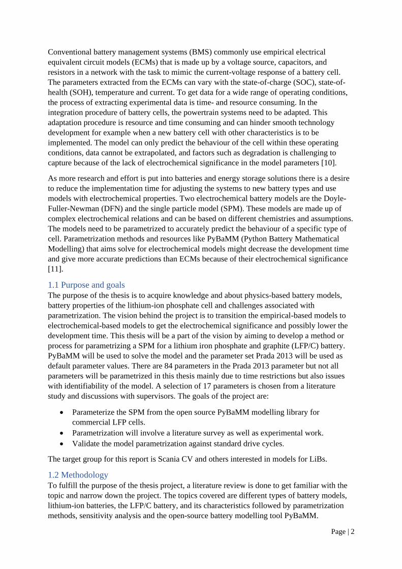
compositions. A Ragone plot with different battery types can be seen in Figure 4.
Page | 7
Figure 4, Ragone plot [7]
One type that has gotten a lot of focus within the automotive market is the lithium-ion
batteries for on-board storage solutions [13]. From the Ragone plot in Figure 4, lithium-ion
batteries (LiB) have a relatively high specific power and specific energy density. In the next
part, more information about lithium-ion batteries will be covered.
2.1.1 Lithium-ion batteries
Due to their high energy and power densities, the LiB technologies are leading in the new
generation of EVs and plug-in hybrid electric vehicles (PHEV) [12]. Common kinds of LiBs
found in electrical vehicles are Lithium Cobalt Oxide (LCO), Lithium Manganese Oxide
(LMO), Lithium Iron Phosphate (LFP) and Lithium Nickel–Manganese–Cobalt Oxide (NMC)
[6]. Different electrode materials have different advantages like lower cost, higher thermal
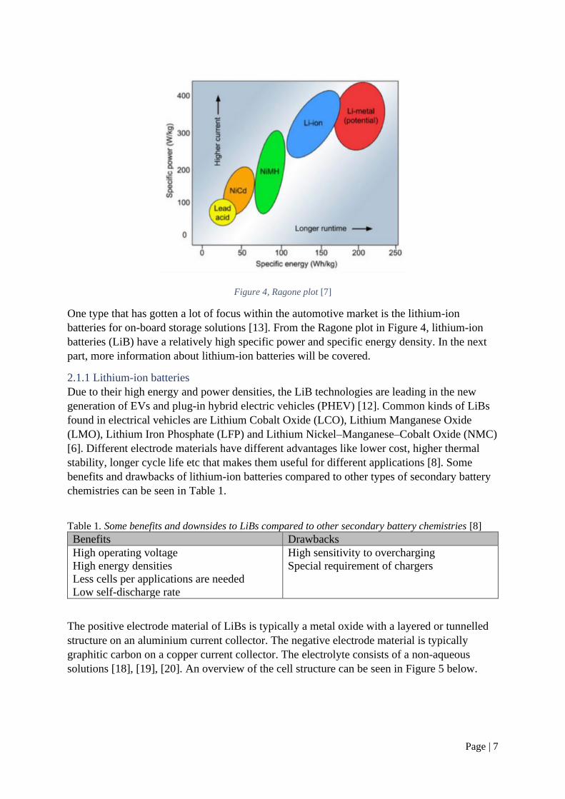
stability, longer cycle life etc that makes them useful for different applications [8]. Some
benefits and drawbacks of lithium-ion batteries compared to other types of secondary battery
chemistries can be seen in Table 1.
Table 1. Some benefits and downsides to LiBs compared to other secondary battery chemistries [8]
Benefits Drawbacks
High operating voltage
High energy densities
Less cells per applications are needed
Low self-discharge rate
High sensitivity to overcharging
Special requirement of chargers
The positive electrode material of LiBs is typically a metal oxide with a layered or tunnelled
structure on an aluminium current collector. The negative electrode material is typically
graphitic carbon on a copper current collector. The electrolyte consists of a non-aqueous
solutions [18], [19], [20]. An overview of the cell structure can be seen in Figure 5 below.

Page | 8
Figure 5, Lithium-ion cell [21]
Intercalation is a property of some electrode materials where the crystal structure allows the
lithium ions to be inserted and removed without changing the materials structure significantly.
The intercalation electrode stays intact during cycling unlike conversion electrodes where the
electrodes are degraded and reformed upon cycling. This reversible
intercalation/deintercalation reduces the problem of dendrite formation of lithium which
provides improvements in safety and cyclability compared to other batteries [18], [19], [20].
During the charge-discharge process, the lithium ions are inserted or extracted from the layers
of the active material [22]. This can be seen in Figure 6 below.
Figure 6, Charging and discharging a LiB. During discharge the lithium ions (purple) are released and
transported through the electrolyte to the cathode. Electrons travel through the wire to the cathode [22].
The electrolyte is not stable for the cell voltage and decomposes to form a passivation layer,
called solid electrolyte interface (SEI), at the negative electrode [23].
2.1.2 Lithium iron phosphate and graphite characteristics
One type of LiB has lithium iron phosphate as positive electrode material and graphite as
negative. These lithium iron phosphate and graphite cells are usually called LFP cells. The
lithium ions can be intercalated in the LFP and graphite structure [18], [19], [20].

Page | 9
The main electrochemical reactions taking place in this cell during charge and discharge can
be seen below. The reactions are stated during discharge.
Reduction: 𝐿𝑖(1−𝑥)𝐹𝑒𝑃𝑂4 + 𝑥 ∙ 𝐿𝑖+ + 𝑒− → 𝐿𝑖𝐹𝑒𝑃𝑂4
Oxidation: 𝐿𝑖𝑥𝐶6 → 𝑥 ∙ 𝐿𝑖+ + 𝐶6 + 𝑒−
Overall reaction: 𝐿𝑖(1−𝑥)𝐹𝑒𝑃𝑂4 + 𝐿𝑖𝑥𝐶6 → 𝐿𝑖𝐹𝑒𝑃𝑂4 + 𝐶6
The “x” in the reactions indicate that the material can hold a variable stoichiometry of lithium
between 0-1. From the reactions it can be seen that only the lithium ions move between the
electrodes during charging and discharging. The name, "lithium-ion" batteries comes from
this mechanism [18], [19], [20].
Graphite is a layered compound that consists of hexagonal graphene sheets of atoms. The
sheets are weakly bonded through van der Waals forces [24]. See the structure of a graphite
unit cell in Figure 7.
Figure 7, Crystalline structure of hexagonal graphite showing the stacking of graphene sheets and the unit cell
[24]
The LFP/C cell differs from most other LiBs with its flat OCV-curve. See the OCV-curves of
LFP/C, NMC/C and NMC/LTO in Figure 8 below.

Page | 10
Figure 8, Typical OCV vs SOC for different lithium-ion batteries [21]
The OCV curve provides important thermodynamic information of the electrode properties
after relaxation of kinetic processes. The LFP electrode has a very flat OCV curve during
lithium intercalation/deintercalation through most of the two-phase reaction in the range
between x=0 to x=1 in LixFePO4 at room temperature [25], [26]. Two-phase regions are
shown as voltage plateaus while the slopes show the phase transitions according to Gibbs’
phase rule. The small “bumps” that can be seen in Figure 8 comes from the graphite
electrodes staging phenomenon when Li is intercalated into the graphite layers. The full cell
OCV-curve mainly exhibit the graphite characteristics [27], [19]. The flat OCV-curve in
combination with path dependence [28] and inherent hysteretic behaviour [29] [26], makes
the SOC difficult to determine with OCV-monitoring. The relationship between SOC and
OCV is essential for battery modelling [30] and to control cell performance in battery
management systems (BMS) [31], [27].
2.2 Battery models
When the demand for electric, hybrid electric and plug-in hybrid electric vehicles increases,
further understanding and development of the batteries are needed to make more accurate
predictions and estimations of the battery. Battery models are commonly used in BMS to
make predictions and estimations about the cell. They are used to understand behaviour,
discover new designs and usage scenarios for batteries. Information like the state of health
(SOH), SOC and their power limits are important to understand changes in the cell like ageing
to increase the lifetime of the cell. This information can help companies to protect and use the
batteries in the best way and estimate the remaining performance [32]. Depending on which
information is desired, there are different models to use, for example atomistic models for
material optimization, continuum electrochemical engineering models to understand drive
performance and manufacturing and techno-economical models that can be used to
understand lifecycle impacts and costs [33]. To estimate the internal states for control
systems, empirical ECMs are often used although there is a desire to integrate physics-based
models with this aim.
The physics-based models are based on parameters with electrochemical meaning which can
provide insights in the different electrochemical phenomena inside the battery. Two examples
of physics-based models are the Doyle-Fuller-Newman (DFN) and the Single particle model
(SPM). A very common type of empirical models is called Equivalent circuit models (ECM).

Page | 11
2.2.1 Equivalent circuit models
ECMs are used to mimic a cell for a set usage. ECMs can be build-up of resistors, capacitors,
inductors, constant phase elements in different configurations. Figure 9 shows a simple
schematic of a part of an electric circuit with resistors (R,s and R,p) and a capacitor (C).
Figure 9, A simple schematic of a part of an electric circuit
By adding more elements, the model can generate more accurate and precise simulations of
the battery behaviour. The disadvantage of more elements in the equivalent circuit is that
more information about the cell is needed for parameterization and the CPU time for
calculations is increased [34].
The empirical model can become very well adapted to the battery and give an accurate
description, but it needs to be tested for all possible scenarios of which the cell should be
used. This is a time-consuming process, which can take months to years. Because of the
simple model structure, relatively low computational burden, and rather easy parametrization
process, ECMs are used for a wide range of industry applications [35]. The simplicity of the
model is also restricting it from describing the physical meaning of the states and parameters
in the cell. The model is only applicable within the scenarios that it has been tested for, it is
hard to extrapolate from data and explain what is physically going on. Processes like ageing
are also difficult to account for in the model which could lead to unwanted effects of
operation. The adaptation needs to be done again and new empirical data must be collected
[35].
2.2.2 Doyle-Fuller-Newman model
The Doyle-Fuller-Newman model (DFN), also called pseudo-two-dimensional (P2D) model
or the Newman model is an electrochemical model that is based on the porous electrode
theory and contains a large number of parameters with physical meaning. This can give a
deeper understanding into processes taking place inside the battery than the ECMs can
provide. Since the DFN model is based on governing physics-based relations and conditions,
it can give more insights into the processes and internal states of the battery, and it is not
limited by a pre-defined scenario window as the ECMs. It is also possible to extrapolate from
these models, adapt and parametrize them to different battery chemistries since they are based
on the same governing equations.
The model have inputs regarding thermodynamic, geometric and kinetic properties of the cell
to be able to describe a specific cell [36]. The accuracy of the input parameters has a large
impact on the reliability of the DFN and other physics-based models. Not all parameter values
can be transferred between cell type, chemistries and sizes, therefore a main challenge in

Page | 12
battery modelling is to find a set of parameters which can and cannot be transferred and how
to find the values needed [36]. To identify electrochemical parameters in a fast and accurate
manner is a vision of many engineers and researchers [35].
The model is complex and is described by a set of highly coupled nonlinear partial differential
equations. This makes it too computationally complex for some applications, like today´s
BMS. For these cases, simpler electrochemical models are of interest.
The governing equations of the DFN are related to charge conservation, molar conservation
and electrochemical reactions. The boundary conditions are the current, concentration in
electrolyte, concentration in electrode active material, reference potential and initial
conditions [36], [37], [38].
2.2.3 Single particle model
A physics-based model that is simpler than the DFN model is the Single Particle model
(SPM). The SPM describes the main phenomena taking place in a Li-ion cell: solid state
diffusion, intercalation and de-intercalation and conduction. It neglects the diffusion in the
electrolyte. See a simple schematic of a battery with the SPM in Figure 10.
Figure 10, (a) Structure of a Li-ion cell: (I) negative current collector; (II) anode; (III) separator; (IV) cathode;
(V) positive current collector. (b) single-particle model schematic [39]
It is assumed that all the particles in the electrode behave the same way and that it is sufficient
to solve the model for one particle. This assumption allows for a considerable simplification
in the model structure and dimension and is generally considered to be acceptable at current
rates (C-rates) up to 1 – 2 C, when electrodes are thin and highly conductive. Following the
assumption, the diffusion and intercalation phenomena occur in a uniform manner in the
electrodes, making it possible to model the electrodes as two spherical particles. This leads to
a simpler version of the DFN model [37]. For several applications with energy optimized
batteries, such as electric vehicles, the average C-rates are lower than 1C [10].
The SPM is not as computationally demanding as the DFN, but it can give more insights into
the physics taking place inside of the cell than ECMs.
Page | 13
2.3 Parametrization of a model
While models consist of mathematical relationships and parameters that together describe a
system, parametrization is related to finding the values of the parameters that makes the
model describe the system in an acceptable way.
The accuracy of the parameters that build up the model have a strong impact on the reliability
of the model. The parameters are specific to the cell design, geometry, and chemistry so not
all parameters can be transferred between cells. Finding a suitable set of parameters that can
simulate a desired aspect of a cell is a challenging task for battery modelling. To find a
suitable set of parameter values, different methods can be used. One method is to fit the
simulation and the model to experimental data such as terminal voltage. This method might
not be feasible without good initial guesses because of the large number of parameters and the
complexity of the model. Secondary, parameter values can be found in literature but there is a
risk of poor model predictions if the values in different sources have different conditions. A
third method would be to measure the parameters experimentally. This could potentially give
more accurate model predictions for the cell but it needs robust approaches and might be
technically complicated and time consuming [36].
A structural property of a model is its identifiability. That a model is identifiable means that
the different parameter values must create different probability distributions of the model
output. When the same model output can be attained with different parameter values, the
model is non-identifiable. A model can be identifiable within certain restrictions. The
requirements for the restriction are called identification conditions [40]. If there is a risk for
co-dependency between parameters, then it can be difficult to have a model or find
requirements where it is identifiable.
2.3.1 Related work
There are several papers available that describes different methods to estimate the parameters
in ECM [41]. Methods to estimate the parameters in the DFN and SPM are scarce. Some
parameters in these electrochemical-based models are possible to find through experiments
but the measurements needed are complicated. The electrochemical models also involve a
larger number of parameters compared to the ECM which makes the estimation more
computational complex. The Gauss-Newton method for non-linear optimization and
homotopy optimization has been used to estimate parameters in the SPM. QR factorisation is
used in the sensitivity analysis for the DFN model in [41] where non-linear least-square
optimization is used to parametrize the sensitive parameters.
2.3.2 Target parameters
While conducting analysis on electrochemical systems, the parameters describing the system
can be grouped into different properties that they are related to, for example into physical,
chemical and electrochemical [36]. In [41] the parameters of the DFN model is divided into
thermodynamic and kinetic parameters. In [35] the groups are geometric, transport and
concentration. The parameters have also been grouped regarding to which phenomena they
are related like diffusive phenomena, intercalation and equilibrium related [39].
The parameter set called Prada 2013 that can be used in simulations with PyBaMM is a
collection of parameters that can be used for LFP/C cells. The parameters in the set orgins
from three different sources [12], [36],[42]. There are in total 84 parameters in the parameter
Page | 14
set that will give different effects on the simulations with PyBaMM [43]. A table with all
parameter values in the Prada 2013 parameter set can be found in Appendix A.
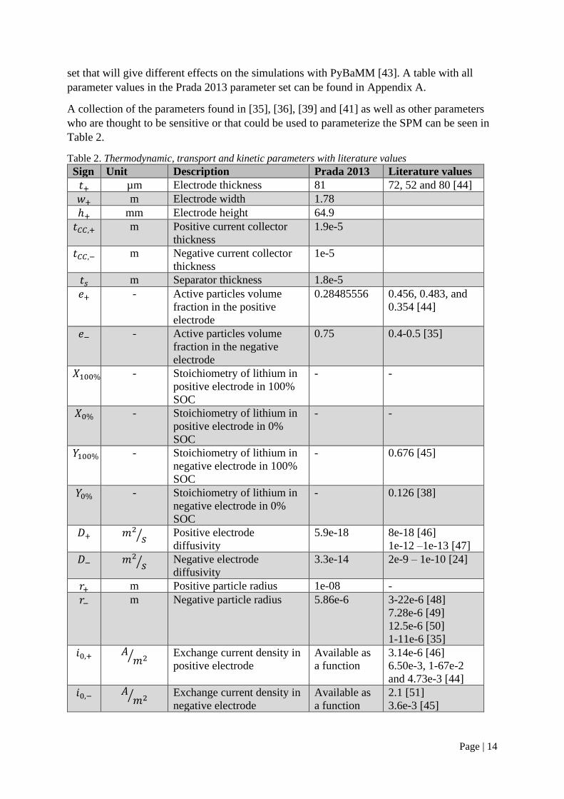
A collection of the parameters found in [35], [36], [39] and [41] as well as other parameters
who are thought to be sensitive or that could be used to parameterize the SPM can be seen in
Table 2.
Table 2. Thermodynamic, transport and kinetic parameters with literature values
Sign Unit Description Prada 2013 Literature values
𝑡+ µm Electrode thickness 81 72, 52 and 80 [44]
𝑤+ m Electrode width 1.78
ℎ+ mm Electrode height 64.9
𝑡𝐶𝐶,+ m Positive current collector
thickness
1.9e-5
𝑡𝐶𝐶,− m Negative current collector
thickness
1e-5
𝑡𝑠 m Separator thickness 1.8e-5
𝑒+ - Active particles volume
fraction in the positive
electrode
0.28485556 0.456, 0.483, and
0.354 [44]
𝑒− - Active particles volume
fraction in the negative
electrode
0.75 0.4-0.5 [35]
𝑋100% - Stoichiometry of lithium in
positive electrode in 100%
SOC
- -
𝑋0% - Stoichiometry of lithium in
positive electrode in 0%
SOC
- -
𝑌100% - Stoichiometry of lithium in
negative electrode in 100%
SOC
- 0.676 [45]
𝑌0% - Stoichiometry of lithium in
negative electrode in 0%
SOC
- 0.126 [38]
𝐷+ 𝑚2
𝑠⁄ Positive electrode
diffusivity
5.9e-18 8e-18 [46]
1e-12 –1e-13 [47]
𝐷− 𝑚2
𝑠⁄ Negative electrode
diffusivity
3.3e-14 2e-9 – 1e-10 [24]
𝑟+ m Positive particle radius 1e-08 -
𝑟− m Negative particle radius 5.86e-6 3-22e-6 [48]
7.28e-6 [49]
12.5e-6 [50]
1-11e-6 [35]
𝑖0,+ 𝐴𝑚2⁄ Exchange current density in
positive electrode
Available as
a function
3.14e-6 [46]
6.50e-3, 1-67e-2
and 4.73e-3 [44]
𝑖0,− 𝐴𝑚2⁄ Exchange current density in
negative electrode
Available as
a function
2.1 [51]
3.6e-3 [45]

Page | 15
𝑘+ 𝑚2.5𝑚𝑜𝑙0.5𝑠 Reaction rate coefficient -
-
𝑘− 𝑚2.5𝑚𝑜𝑙0.5𝑠 Reaction rate coefficient - 1e-11 – 2e-10 [35]
𝜎+ 𝑆𝑚⁄ Positive electrode
conductivity
0.33795074 10e-7 –10e-8 [46]
1e-7 [47]
0.001-1 [52]
𝜎− 𝑆𝑚⁄ Negative electrode
conductivity
215.0 (2-1)e5 [47]
2-3e5 [53]
3e5 [46]
100 [45]
R Ω Cell resistance -
Diffusivity
The transport parameters are linked to the cell´s capability to transport particles and ions.
Diffusion is the movement along concentration gradients. Atoms move in a predictable
fashion to eliminate concentration differences and produce a uniform and homogeneous
composition [53]. Nernst Plack equation (Equation 4) describes the diffusion in electrolytic
solutions [47].
The intercalation process of lithium ions into electrodes involves several processes like the
diffusion through the electrolyte, migration in the surface film, charge transfer at the
electrode/electrolyte interface followed by the diffusion in electrode. While using the SPM,
the mass transport in the electrolyte is assumed to be instantaneous and the transport in the
electrodes are most important. In carbon electrodes the mass transport of lithium ions is
regarded as a diffusive process and since the diffusion process in solids is generally slow, the
rate of diffusion is limiting the overall reaction rate [24]. The diffusion coefficient, or
diffusivity, of Li-ions in the electrode´s active material can be seen as a parameter of interest
for a sensitivity analysis and parameter estimation of LiBs [41], [50], [35], [39], [24].
There are several methods to determine the diffusion coefficients of lithium in solids. Some
examples are galvanostatic intermittent titration technique (GITT), current pulse relaxation,
potential step chronoamperometry and AC impedance spectroscopy. A precise determination
of the diffusivity is generally difficult to conduct, and the results depend on which kind of
material and additives that make up the electrodes and the technique that is used. For some of
these techniques, the variation of the open-circuit potential with lithium composition and the
surface area of the sample need to be highly accurate [24].
Particle radius
The particle radius of the electrode material depends on the production. To offset the solid-
phase diffusion limitation, the particle radius of the LFP active materials are usually prepared
in nano-size particles [47]. The reversibility of the intercalated lithium ion in graphite is
strongly dependant on the particle size of graphite [54]. Scanning electron microscopy (SEM)
can be used to find a particle size distribution [44].
Reaction rate
The reaction rate in the electrode is an important kinetic parameter because it is linked to the
rate limiting processes within the cell. The reaction rate is not an individual parameter in the
Prada 2013 parameter set but is expressed through the exchange current densities in the

Page | 16
electrodes. Through the Butler-Volmer and Arrhenius equations, the connection between
reaction rate and the exchange current density can be found.
𝑗(𝜂) = 𝑗0 ∙ {𝑒𝑥𝑝 (𝛼𝑎𝐹𝜂
𝑅𝑇) − 𝑒𝑥𝑝 (
−𝛼𝑐𝐹𝜂
𝑅𝑇)} (5)
The Butler Volmer equation (5) describes the current density as a function of the
overpotential. 𝑗0 is the exchange current density. F is the Faraday constant, η is the
overpotential, R is the ideal gas constant, T is the temperature, and α the transfer coefficient
(one for the anode and one for the cathode) [16].
Arrhenius equation (6) predicts kinetics based on thermal activation [47].
𝑟𝑎𝑡𝑒 ≈ 𝑒(−∆𝐺
𝑘𝐵𝑇) (6)
In Arrhenius equation, ∆𝐺 is the change in Gibbs free energy, kB is the Boltzmann constant
and T is the temperature.
Exchange current density
The exchange current density is the current density when the electrode is at equilibrium. Since
the electrode is at equilibrium the reduction and oxidation take place at the same rate and
there is no net current density. The exchange current density is dependent on the temperature,
electrolyte concentration and particle surface concentration. In PyBaMM, the exchange
current densities are expressed as functions of these parameters.
Pulse test and Electrochemical Impedance Spectroscopy (EIS) are alternative methods to find
information about exchange current density, activation energy and reaction rate [55]. The
exchange current density can be obtained from Tafel plot that can be made from the Butler-
Volmer Equation (5)
A functional form of the exchange current can be used. When assuming that 𝛼=0.5 it takes the
form of Equation 7 [36].
𝑗0 = 𝑘 ∙ √𝑐𝑒 ∙ 𝑐𝑠 ∙ (𝑐𝑠𝑚𝑎𝑥 − 𝑐𝑠) (7)
In Equation 7, 𝑗0 is the exchange current density, k is the reaction rate, 𝑐𝑒is the electrolyte
concentration, 𝑐𝑠 is the electrode surface concentration and 𝑐𝑠𝑚𝑎𝑥 is the maximum electrode
surface concentration.
Electrode conductivity
The internal resistance of the cell is regarded as an important parameter in order to make a
parametrization of a battery cell [39]. The cell resistance is not included as a parameter in the
Prada 2013 parameter set, but it is related to the conductivities. How the resistance in a wire is
related to its conductivity can be seen in Equation 8.
𝑅𝑐𝑒𝑙𝑙 =𝑙
𝜎𝐴 (8)
𝑅𝑐𝑒𝑙𝑙 represents the internal resistance, A represents the area, 𝜎 represents the conductivity
and 𝑙 represents the length of the wire.
The electrical conductivity of an electrode is a material property that determines how well the
material will conduct electricity. LFP is known to have poor electrical conductivity [46],[47].

Page | 17
Several ways to increase the electrical conductivity of the LFP electrode has been made such
as adding or coating carbon to LFP electrodes and/or current collectors to increase the
electrical conductivity of the electrode and lessen the contact resistance. Factors like the
carbon content, the quality of the carbon coating, calendaring, and doping materials have
impacts on the electrical conductivity. The low electrical conductivity can result in a
considerable ohmic drop within the electrode [46], [52], [47].
Graphite has a higher electrical conductivity than LFP. The electrical conductivity is closely
related to the morphology of the graphite. The smaller the particle size and the higher the
surface area, the lower the conductivity [56].
3. METHOD AND THEORY
3.1 Method overview
In order to parametrize a LFP/C cell for the SPM, a step-wise procedure is taken. Starting
with a literature review, followed by a simple sensitivity analysis, experiments, numerical
simulations and parameter estimation.
The literature values available in the Prada 2013 parameter set was be used as initial
guesses/default values while some targeted parameters, that is found in literature, will be
estimated in order to find more parameter values that better describe the system. This will be
done through conducting a number of experiments form which the values will be calculated
from or found through a curve fitting procedure. A summarized workflow can be seen in
Figure 11.
Figure 11, workflow to find optimal parameter values.
3.1.1 Literature review
To fulfil the purpose of the thesis project, a literature review is done to get familiar with the
topic and narrow down the project. The topics covered are different types of battery models,
lithium-ion batteries, the LFP/C battery, and its characteristics followed by parametrization
methods, sensitivity analysis and PyBaMM. The databases used are mainly KTH Library and
Google Scholar.
Form the literature study, three types of experiment are chosen because parameters are able to
be extracted from the experimental data or used as basis for a curve fitting procedure.
3.1.2 Sensitivity analysis
A sensitivity analysis was conducted to check if the parameters are sensitive for the
experiments.
For the experiments used to find the transport and kinetic parameters, a sensitivity analysis of
the simulated response of a disturbance of ±10 % in each parameter was done. To disturb the
parameters by 10 % might in reality be an unrealistic disturbance if for instance, the
parameters could only be within a smaller range. An alternative method is to find within

Page | 18
which ranges the parameters are usually found and then disturb the parameters within that
range. The simpler method is chosen due to the restricted amount of time.
The SPM is based on several non-linear differential equations, like the OCV-curves and the
Butler-Volmer equation [50]. Some equations and parameters show linear characteristics in
some parts, but the model is mostly non-linear. To care for the non-linearity, it is possible to
grid the problem and select several different points in the SOC or temperature to see where
the parameters are the most sensitive. A convenient way to do this would be to check in three
different points of the SOC. The sensitivity is taken in targeted SOC regions in the beginning,
the centre and end of the simulation.
3.1.3 Numerical simulation
Simulations with the SPM were performed using the open-source software package Python
Battery Mathematical Modelling (PyBaMM). PyBaMM can be used to solve continuum
battery models using asymptotic analysis and numerical methods [11]. For the simulations in
this thesis, PyBaMM v. 0.4.0 was used to solve the SPM without electrolyte. The Prada 2013
parameter set was be used as default values for the parameters. The SPM without electrolyte
is based on the equations described in [37].
3.1.4 Experimental setup
LFP/C cells of the model HTPFR18650-1100mAh-3.2V were be used in the experiments. The
technical parameters of the cylindrical cells received from the producers’ data sheet can be
seen in Figure 12.
Figure 12, Major technical parameters [57]
A total of 4 cells were used in the experiments. To see if the cells were working well, the cell
voltage is tested with a multimeter before the cells are entered into the cell holder and tests
started.
The cells were placed in a cell holder which is built for the experiment, see setup in Figure 13.
This is a four-probe setup.

Page | 19
Figure 13, Cell setup
The cells and the holder were then placed in a climate chamber which keeps a constant
temperature of 25 °C in steady state conditions. There was a power source that can do
potentiostatic and galvanostatic experiments, a control PC with EC-lab software which was
used to perform the monitoring and control of the system. A booster was used to access higher
currents.
3.1.5 Parameter fitting
The experiments were conducted to get the data and the parameters were extracted through
methods found in the literature, mostly [39]. Curve fitting by editing the parameter values of
the Prada 2013 parameter set to make the simulation in PyBaMM match the experimental data
were also performed. A non-linear least squares method was used to fit a function to data via
the curve fit method of the Python library scipy.optimize [58]. Scipy version 1.5.2 was used.
The formula for a least square method for a simple line, with the form y=mx+b with m being
the slope and b being the intercept with the y-axis, can be seen in Equation 9.
𝑦 =𝑁∑(𝑥𝑦)−∑𝑥∑𝑦
𝑁(𝑥2)−(∑𝑥)2𝑥 +
∑𝑦−𝑚∑𝑥
𝑁 (9)
3.2 Experimental methods
The experiments were inspired by the ones described in [39] where experiments were
performed on lithium-titanate cells in order to extract parameters related to the equilibrium,
diffusive and intercalation phenomena. In the paper, a reformulation of the SPM was
conducted to get a minimum amount of group parameters. Three non-intensive methods were
proposed to identify the parameter values that would be sufficient to parameterize the
reformulated SPM. The experiments were made so that parameter values could be extracted
through curve fitting methods and equations. These procedures seemed promising and were
adapted for the LFP/C cells investigated in this thesis. The parameters were also adapted to
match the once available in PyBaMM.
The geometric parameters 𝑡+, 𝑤+, ℎ+, 𝑡𝐶𝐶,+, 𝑡𝐶𝐶,− and 𝑡𝑠 will be found by measuring them
during a cell opening. They are linked to the volume of the electrode and therefore also the
capacity of the cell. The geometrical parameters can also be related to the resistance in the cell

Page | 20
according to Figure 2. The other thermodynamic parameters 𝑒+, 𝑒−, 𝑋100%, 𝑋0%, 𝑌100% and
𝑌0% will be found through a curve fitting procedure similar to the one described in [39]. The
transport and kinetic parameters will undergo a sensitivity analysis and a curve fitting
procedure to find the parameter values. See the theoretic background behind the experiments
chosen and the block diagrams for the cycling, GITT and pulse test in the following sections.
3.2.1 Thermodynamic parameters via low-rate cycling
Depending on the desired resolution, the OCV can be derived from galvanostatic intermittent
titration technique (GITT). This procedure is done by moving small steps in the SOC window
with low currents, like C/20. This procedure can be relatively time consuming, not unusual
with week-month periods, demanding depending on the number and sizes of the SOC steps
that are taken. To get information of the OCV in a faster manner, a cell can be cycled at very
low currents, such as C/25, to generate a pseudo-OCV curve [39], [27]. The low current is
used to minimize kinetic contributions, reduce ohmic heat generation and electrode
polarization [27]. It is assumed that the reactions happen at equilibrium state and that within a
part of the SOC window, a pseudo OCV curve can be found [59]. Hysteresis can however still
occur in the pseudo-OCV curves that are received from low rate cycling [60].
In order to determine parameters such as the capacities of the two electrodes, cycling tests
with a low C-rate was conducted in a procedure that is influenced by a method presented in
[39]. The low-rate tests include a full discharge followed by a full charge with a constant and
low C-rate of C/30. This experiment makes it possible to determine the capacity of the full
cell as well as the OCV characteristics. When operating in the SOC-window it is important to
consider the different capacities of the electrodes. SOC is the ratio between the capacity and
the maximum cell capacity [49]. A block diagram of the cycling test can be seen in Figure 14.
Figure 14, Low-rate cycling block diagram
Three cells were be tested with this procedure, some at C/30 and some at C/50 to make sure
that the cell is in equilibrium.
3.2.2 Transport related parameters via GITT
GITT is a procedure useful to retrieve several kinds of parameters. The GITT procedure
consists of a series of current pulses, each followed by a relaxation time where no current
passes through the cell. The current is positive during charge and negative during discharge.
As mentioned in the Background several different methods can be applied to find the
diffusion coefficient/diffusivity in the solid phase. The choice of method can also affect the
values of the diffusion coefficient. For this thesis, only one method will be utilized. A series

Page | 21
of GITT tests can be used to find the solid diffusion coefficients of the electrodes. This is
performed by a sequence of constant current discharge at low C-rate, followed by resting
phases that brings the cells back to equilibrium. The experiment set up was influenced by the
method used in [39] where test are done on a lithium titanate cell. In [39], the diffusion
coefficient was extracted with a curve fitting procedure that assumed that the cell reaches
equilibrium potential after a relaxation period. See Figure 15 for the desired appearance of the
GITT pulse.
Figure 15, Shape of GITT pulse [39]
In Figure 15, the change in voltage ∆𝑉𝑡 in the pulse and ∆𝑉𝑠 which is the voltage in the
equilibrium state after the pulse can be seen as well as 𝜏 which is the time of the pulse.
Equation 10 shows a general way to calculate the diffusion coefficient from GITT
experiments for half cells. 𝑅𝑖 is the internal resistance.
𝐷𝑖 =4
𝜋𝜏(𝑅𝑖
3)2
(∆𝑉𝑠
∆𝑉𝑡)2
(10)
By finding ∆𝑉𝑡 and ∆𝑉𝑠 for different parts of the SOC window, the diffusivity that is
normalized with the particle radius can be found through a curve fitting procedure. Another
more flexible approach to find values that are related to the diffusive phenomena is by fitting
the relaxation region from the experimental data to simulated values. To compare the
simulated and experimental data, these conditions need to be fulfilled:
1. The cell should be at rest in the start of the data set.
2. The current is the same in simulation and experiment.
3. The voltage should be the same in the start for the simulation and experiment.
The time needed for the cell to relax depends on the cell type [49]. While the relaxation time
used in [39] was 15 minutes, a rest time of 2 hours was initially applied for the LFP/C cell.
After finding that the cell did not reach equilibrium within the 2 hours, the relaxation time
was extended to 4 hours. Due to the flat OCV curve of the LFP/C cell, a relative long time is
required to get to equilibrium conditions. Because of this the cell is found not be relaxed even
after 4 hours of rest so the latter approach is chosen.

Page | 22
The apparent diffusion coefficients and OCV characteristics can, as mentioned earlier, be
found by performing GITT. By making GITT at different cell configurations like full cell,
half-cell and three electrode set-up, the parameters can be compared [36] but only full cell test
will be done in this work as is described in [39].
The block diagram of the GITT test can be seen in Figure 16. The C/20 pulses are the GITT
pulses while the C/3 pulses are used to move to another SOC level.
Figure 16, GITT block diagram
3.2.3 Kinetic parameters via pulse test
In [39] a pulse test consisting of a series of pulses with different C-rates were proposed as a
method to find the reaction rate in the positive electrode, negative electrode and the resistance
in the cell. Even though the reaction rates at each electrode nor the cell resistance are
explicitly tuneable parameters in PyBaMM, the experimental setup does seem feasible to give
the desired information. This was because the reaction rates in the electrode was related to the
exchange current density at each electrode and the internal cell resistance was connected to
the electrode conductivity which was tuneable in PyBaMM. The reaction rate was a factor
that describes the exchange current density according to Equation 7. By adding a factor 𝑘𝑓 to
the equation, the effect on the exchange current density by changing the reaction rate can be
found. The Equation 7 can be rewritten as Equation 11 for this purpose.
𝑗0 = 𝑘𝑓 ∙ 𝑘 ∙ √𝑐𝑒 ∙ 𝑐𝑠 ∙ (𝑐𝑠𝑚𝑎𝑥 − 𝑐𝑠) (11)
With Equation 11, it is possible to find the 𝑘𝑓 value that makes the simulation match the
experimental data from the pulse test. The block diagram for the pulse test can be seen in
Figure 17.
est
5 min
harge
0
0 min
we . 5
est
h
harge
min
est
h
ischarge
0
0 min
we . 5
est
h
ischarge
min
est
h
epeat 9 times
epeat 9 times

Page | 23
Figure 17, Pulse test block diagram
In [39] the parameter values can be related to the SOC and the current rates at the pulses. In
this thesis only the first C/2 pulses will be used for fitting the values due to time restrictions.
3.3 Sensitivity analysis
For the GITT and pulse test a sensitivity analysis was performed to find how sensitive
parameters are in relation to one another. The parameter values were changed by ±10 % and
the effect in different regions of the voltage profile will be investigated for each experiment.
Some parameters show linear characteristics in some parts, but the model is mostly non-
linear. To care for the non-linearity, it is possible to grid the problem up and select several
different points in the grid to see where the parameters are the most sensitive. This was done
by selecting pulses in three different points of the grid: the beginning, centre and end. The
sensitivity of the parameters 𝐷+, 𝐷−, 𝑟+, 𝑟−, 𝑘𝑓+, 𝑘𝑓−, 𝜎+ and 𝜎− 𝑤ill be found for GITT and
pulse test simulations.
3.3.1 Sensitivity analysis for GITT
By shifting the cell from equilibrium with a small current during a long time, the ohmic and
kinetic effect on the cell voltage want to be minimized while the effect from transport
phenomena is maximized. The most relevant aspect to look at is the relaxation time and the
region where the cell relaxes. In principle it would be possible to find the parameter values
from the pulse region too. The reason why the pulse region was not included in the fit was
because when the current is not zero, the deviation from equilibrium and the equilibrium itself
is time-dependant which complicates the mathematical description taking place. When the
current is zero, only the deviation from equilibrium is time-dependant. Therefore, the three
C/20 GITT pulses were analysed based on their change in the dynamic relaxation region. A
simulation of the GITT procedure during discharge can be seen in Figure 18. The pulses
number 2, 6 and 9 were chosen to investigate to see the sensitivity in the beginning, middle
and end of the SOC window.

Page | 24
Figure 18, GITT simulation based on Prada 2013 parameter set
The period of interest was from the bottom of the pulse, where the relaxation starts, until the
simulation have reach equilibrium at around half of the rest time until the next pulse.
A linear first order system can be described with this differential equation:
𝑇𝑑𝑦
𝑑𝑡+ 𝑦 = 𝐾𝑢 (12)
In Equation 12, K is the system´s steady state gain and the T is the time constant. The shape
of the relaxation is very similar to the step answer of a first order linear time invariant system,
see Figure 19. It was therefore assumed that the dynamic relaxation region acts like a first
order linear time invariant system.
(a)
(b) [61]
Figure 19, (a) Zoom in on dynamic relaxation region (b) The step answer from a 1st order linear time
invariance.
The dynamic relaxation resembles the response of a step answer which can be seen in
Equation 13 [61].

Page | 25
𝑦(𝑡) = 𝐾𝑢𝑠𝑡𝑒𝑝 ∙ ( − 𝑒−𝑡
𝜏⁄ ) (13)
By changing the parameters one by one, ± 10% from the original values, the changes of the
disturbance can be seen for K and 𝜏. By finding the K and 𝜏 values when no disturbance is
done and then a measurement of the sensitivity could be calculated with Equation 14.a and
14.b.
𝑆𝑒𝑛𝑠𝑖𝑡𝑖𝑣𝑖𝑡𝑦𝜏 =|𝜏𝑝𝑎𝑟𝑎𝑚,0.9−𝜏𝑝𝑎𝑟𝑎𝑚,1.1|
𝜏𝑝𝑎𝑟𝑎𝑚,1 (14.a)
𝑆𝑒𝑛𝑠𝑖𝑡𝑖𝑣𝑖𝑡𝑦𝐾 =|𝐾𝑝𝑎𝑟𝑎𝑚,0.9−𝐾𝑝𝑎𝑟𝑎𝑚,1.1|
𝐾𝑝𝑎𝑟𝑎𝑚,1 (14.b)
3.3.2 Sensitivity analysis for Pulse test
During the pulse test, the pulse was conducted with a higher C-rate than in the GITT test and
at a shorter time. The physical effect of this was that the overpotentials are mostly linked to
activation and ohmic drop. The pulse duration of 10 seconds was on the limit of changing the
cell concentration significantly. It is therefore assumed that concentration overpotentials are
not affecting the pulses. The most interesting feature to capture for this test was the change in
voltage during a pulse.
From the literature review (see Background), the reaction rates (related to the current density)
and the internal resistance in the cell (related to the conductivity in the electrodes) would
affect the depth of the voltage drop. Therefore, the region with the instantaneous voltage
drops is the most interesting feature for the purpose of finding the targeted parameter values.
In [39] the parameter values can be related to the SOC and the current rates at the pulses. For
the sensitivity analysis, three pulses will be analysed for their effect on the voltage depth
during a pulse.
Since the first pulse set is affected by relaxation, as seen in the steep appearance in Figure 20,
the pulses set number 2, 6 and 10 were chosen to investigate to see the sensitivity in the
beginning, middle and end of the SOC window. Only the first C/2 pulse in each pulse set is
analysed.

Page | 26
Figure 20, Pulse test simulation with Prada 2013 parameter set.
3.4 Parameter estimation method
In order to parametrize the SPM described in [37] that is available in PyBaMM, a series of
experimental tests are conducted in a way described in [38] and [10] so that some parameters
can be extracted from the data and through curve fitting. Three tests that describe different
phenomena are conducted: low-rate cycling, GITT and pulse test. The low-rate cycling test
explores the capacity phenomenon. The diffusion phenomenon is explored in the GITT test.
In the pulse test, it is assumed that the diffusion phenomenon do not affect the results since
the pulse is conducted under a short time, and the reaction rates can be explored. The settings
for the experiments can be seen under the Experiment descriptions.
From the sensitivity analysis the parameter´s relative sensitivity is investigated for the GITT
and pulse test. For each experiment, a few parameters have been selected since they are
thought to be sensitive according to literature. For these chosen parameters that are taken from
literature, a sensitivity analysis will be done on the simulations in PyBaMM to find out how
sensitive the parameters are. The sensitivity analysis will be specific for the experiment and
will be described in the section Sensitivity analysis.
For the parameters that are found to be sensitive for each experiment, the parameters will be
tuned to make the PyBaMM simulation fit the experimental data as good as possible. The
output will be three parametrizations: one to find the optimal parameter values for the cycling,
GITT and pulse experiments, respectively. These experimental optimal parameters will then
be part of the new parameter set that will make up the fully parametrized model. The
parametrized model will be validated by comparing the simulations against data that aims to
represent use of LFP/cells in BEV and mild-hybrid vehicles. This will also be compared to the
default parameters found in PyBaMM. The parameters for GITT and Pulse test are found
through a curve fitting procedure.

Page | 27
In order to get optimal values for the targeted parameters, Figure 13 presents how the
parameter values will be found.
Figure 21 shows that the selected parameters are thermodynamic, transport and kinetic
related. The parameter values found from the cell opening and the low-rate cycling will be
used together with default values to find the parameter values of GITT and Pulse test that best
match the experimental data.
Figure 21, parametrization procedure*
*An alternative parametrization procedure can be found in Appendix D.
3.4.1 Cell opening
One cell is opened to measure some geometrical parameters. In Figure 22 (a) and (b) the
measurement of the electrode and current collector can be seen. In order to get the
geometrical parameters, a cell is opened. The cell is opened in a LABmasterPro Eco glove
box from Mbraun by Matilda Klett Hudson at Scania material technology lab.
(a)
(b) Figure 22 (a) and (b), measurement of geometrical parameters

Page | 28
The electrode heights and widths are measured with a mm spaced ruler seen in the lower part
of Figure 22 b. The electrode thicknesses are measured with a micrometer that gives the result
in micrometers on a digital display that can be seen in Figure 22 a. The electrodes in the cell
are rolled upon itself, which is the structure of cylindrical cells, with the electrodes being a
coated layer on top of the current collector as seen in the Figure 23.
𝑡𝑠ℎ𝑒𝑒𝑡
𝑡𝐶𝐶
Figure 23, Measurement of thickness of electrode and current collector. The grey and black rectangles represent
the electrode coating layers and the current collector.
In order to measure the thickness of the electrode coating layer the thickness of the whole
sheet is measured, 𝑡𝑠ℎ𝑒𝑒𝑡. The layer of electrode coating is carefully scraped of using a
scalpel. Some drops of dimethyl sulfoxide are used to loosen up the LFP coating layer while
the graphite only needed the scalpel. The thickness of the current collectors is measured, 𝑡𝐶𝐶.
The thickness of the electrode coatings is calculated as in Equation 15.a and 15.b. The
thickness of the electrodes is considered to include the coating on both sides of the current
collector.
𝑡− = 𝑡𝑠ℎ𝑒𝑒𝑡,− − 𝑡𝐶𝐶,− (15.a)
𝑡+ = 𝑡𝑠ℎ𝑒𝑒𝑡,+ − 𝑡𝐶𝐶,+ (15.b)
The prefix of + and - symbolizes that the sheet and current collector is linked to the positive
and negative electrode.
It was determined with eyesight that the electrode coating was removed from the current
collector. There might still be coating present which will make the 𝑡𝐶𝐶 measurement prone to
error. Therefore, several points on the scraped area are measured to get a mean value. The risk
of damaging the current collector by creating holes in it with the scalpel is also a risk. When
there is a visible hole, that area is excluded from the measuring points.
3.4.2 Low-rate cycling
The thermodynamic parameters from the cycling test are calculated in an order where the
values found for one parameter is used to calculate the next one.
3.4.2.1 Cell capacity
The cell capacity at a certain c-rate can be calculated by Equation 16.
𝑄𝑐𝑒𝑙𝑙 = 𝑡𝑑𝑖𝑠𝑐ℎ𝑎𝑟𝑔𝑒 ∙ 𝐼�̅�𝑖𝑠𝑐ℎ𝑎𝑟𝑔𝑒 (16)
In Equation 16, 𝑄𝑐𝑒𝑙𝑙 is the cell capacity discharged at a certain C-rate, 𝑡𝑑𝑖𝑠𝑐ℎ𝑎𝑟𝑔𝑒 is the time
required to discharge the cell and 𝐼�̅�𝑖𝑠𝑐ℎ𝑎𝑟𝑔𝑒 is the mean current during the discharge. The cell
capacity is calculated from the low-rate cycling test. It is also possible to calculate the cell
capacity during charging as well but only the discharging will be considered in the further
calculations. Figure 24 shows the data from the full cycling test while Figure 25 shows the
discharge part and the applied current.

Page | 29
Figure 24, Low rate cycling (charge and discharge) cell D C/30
Figure 25, Low-rate cycling (discharge) cell D C/30
The nominal capacity, 1.1 Ah of the cell is obtained when the cell is discharged from fully
charged at constant current and 1 C. In the low-rate cycling experiment the cell is discharged
at C/30. The discharge capacity from cell D C/30 will be used for the following calculations.
The SOC is calculated according to Equation 17.
𝑆𝑂𝐶 =𝐼∙𝑡
𝑄𝑚𝑎𝑥 (17)

Page | 30
In Equation 17, I is the current, t is the time and 𝑄𝑚𝑎𝑥 is the maximum capacity of the cell.
The equation is equivalent to finding the ratio between the capacity at a certain time and the
maximum capacity.
3.4.2.2 OCV curve
In [39] it is stated that it is possible to determine the OCV curves as functions of the ion
concentration in the electrode if the electrode material is known and literature is available.
The OCV curves for each electrode are available as a parameter in Prada 2013, the LFP
electrode as a function and the graphite as an array. Since these OCV curves are only for half
cells, they need to be adapted to represent a full LFP/C cell. A wrapper function is used to
make the LFP function to support iterables. Interpolation within the table data of the graphite
is used to get values of the OCV. The SOC window is adapted and normalized between 0-1.
The OCV curves are related to the maximum and minimum concentrations of the individual
electrodes. The values of these parameters will be fitted so that the OCV curve from the
experimental data of the low-rate cycling matches the theoretical OCV functions of the
electrode materials. The analytical OCV curve is set up according to Equation 18.
𝑂𝐶𝑉𝑓𝑖𝑡𝑡𝑒𝑑 = +𝑂𝐶𝑃+(𝑧+,𝑚𝑎𝑥, 𝑧+,𝑚𝑖𝑛) − 𝑂𝐶𝑃−(𝑧−,𝑚𝑎𝑥, 𝑧−,𝑚𝑖𝑛) (18)
The difference between the electrodes OCV curves is found to describe the full cells OCV.
In order to calculate the total available capacity of the individual electrodes the stoichiometry
at 0% and 100 % SOC in both electrodes need to be found through curve fitting. The
capacities of the positive LFP and negative graphite electrode can be calculated as [39]:
𝑄+ =𝑄𝑐𝑒𝑙𝑙
𝑧+,𝑚𝑎𝑥−𝑧+,𝑚𝑖𝑛 (18.a)
𝑄− =𝑄𝑐𝑒𝑙𝑙
𝑧−,𝑚𝑎𝑥−𝑧−,𝑚𝑖𝑛 (18.b)
Where 𝑄+ and 𝑄− are the capacities of the positive and negative electrode, respectively.
𝑧+,𝑚𝑎𝑥 and 𝑧+,𝑚𝑖𝑛 are the stoichiometries at 100% and 0% SOC in the positive electrode.
Alike goes for 𝑧−,𝑚𝑎𝑥 and 𝑧−,𝑚𝑖𝑛 but for the negative electrode. These stoichiometric values
represent how much of the individual SOC window of each electrode that is used in the cell.
The values will be in the range between 0 and 1, where 0 is linked to the lower stoichiometric
value and 1 to the higher. If the entire SOC window of the electrode is used in the cell, the
values will be 0 and 1.
This code was time-consuming to run. In order to reduce the number of times the code should
run, bounds are found by manually changing the values until a reasonable good fit is achieved
between the simulation and the experimental values. Smaller bounds around the manually
found values are then used in the Scipy.optimize.curve_fit function in order to get an
optimized fit.
In the fitting procedure, it is assumed to be of higher importance to get a good fit for the
graphite bumps seen in Figure 26. To accomplish this, different regions of the SOC window
was prioritized in the curve fitting procedure. The regions with the graphite bumps were
prioritized higher while the other regions are weighted lower.
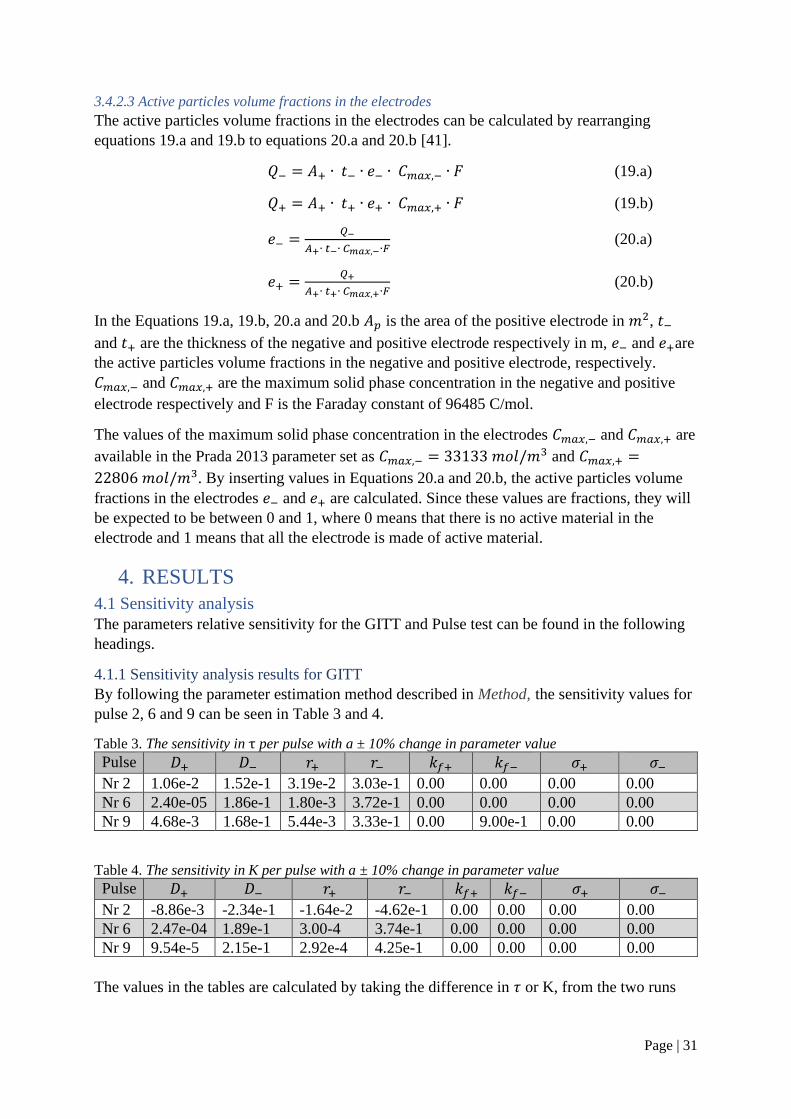
Page | 31
3.4.2.3 Active particles volume fractions in the electrodes
The active particles volume fractions in the electrodes can be calculated by rearranging
equations 19.a and 19.b to equations 20.a and 20.b [41].
𝑄− = 𝐴+ ∙ 𝑡− ∙ 𝑒− ∙ 𝐶𝑚𝑎𝑥,− ∙ 𝐹 (19.a)
𝑄+ = 𝐴+ ∙ 𝑡+ ∙ 𝑒+ ∙ 𝐶𝑚𝑎𝑥,+ ∙ 𝐹 (19.b)
𝑒− =𝑄−
𝐴+∙ 𝑡−∙ 𝐶𝑚𝑎𝑥,−∙𝐹 (20.a)
𝑒+ =𝑄+
𝐴+∙ 𝑡+∙ 𝐶𝑚𝑎𝑥,+∙𝐹 (20.b)
In the Equations 19.a, 19.b, 20.a and 20.b 𝐴𝑝 is the area of the positive electrode in 𝑚2, 𝑡−
and 𝑡+ are the thickness of the negative and positive electrode respectively in m, 𝑒− and 𝑒+are
the active particles volume fractions in the negative and positive electrode, respectively.
𝐶𝑚𝑎𝑥,− and 𝐶𝑚𝑎𝑥,+ are the maximum solid phase concentration in the negative and positive
electrode respectively and F is the Faraday constant of 96485 C/mol.
The values of the maximum solid phase concentration in the electrodes 𝐶𝑚𝑎𝑥,− and 𝐶𝑚𝑎𝑥,+ are
available in the Prada 2013 parameter set as 𝐶𝑚𝑎𝑥,− = 𝑚𝑜𝑙/𝑚3 and 𝐶𝑚𝑎𝑥,+ =
22806 𝑚𝑜𝑙/𝑚3. By inserting values in Equations 20.a and 20.b, the active particles volume
fractions in the electrodes 𝑒− and 𝑒+ are calculated. Since these values are fractions, they will
be expected to be between 0 and 1, where 0 means that there is no active material in the
electrode and 1 means that all the electrode is made of active material.
4. RESULTS
4.1 Sensitivity analysis
The parameters relative sensitivity for the GITT and Pulse test can be found in the following
headings.
4.1.1 Sensitivity analysis results for GITT
By following the parameter estimation method described in Method, the sensitivity values for
pulse 2, 6 and 9 can be seen in Table 3 and 4.
Table 3. The sensitivity in τ per pulse with a ± 10% change in parameter value
Pulse 𝐷+ 𝐷− 𝑟+ 𝑟− 𝑘𝑓+ 𝑘𝑓− 𝜎+ 𝜎−
Nr 2 1.06e-2 1.52e-1 3.19e-2 3.03e-1 0.00 0.00 0.00 0.00
Nr 6 2.40e-05 1.86e-1 1.80e-3 3.72e-1 0.00 0.00 0.00 0.00
Nr 9 4.68e-3 1.68e-1 5.44e-3 3.33e-1 0.00 9.00e-1 0.00 0.00
Table 4. The sensitivity in K per pulse with a ± 10% change in parameter value
Pulse 𝐷+ 𝐷− 𝑟+ 𝑟− 𝑘𝑓+ 𝑘𝑓− 𝜎+ 𝜎−
Nr 2 -8.86e-3 -2.34e-1 -1.64e-2 -4.62e-1 0.00 0.00 0.00 0.00
Nr 6 2.47e-04 1.89e-1 3.00-4 3.74e-1 0.00 0.00 0.00 0.00
Nr 9 9.54e-5 2.15e-1 2.92e-4 4.25e-1 0.00 0.00 0.00 0.00
The values in the tables are calculated by taking the difference in 𝜏 or K, from the two runs

Page | 32
where a parameter is disturbed by ± 10% from its original value, divided by the 𝜏 or K when
the parameters are not disturbed i.e., Equations 14.a and 14.b.
From the Tables 3 and 4 it seems like the electrode conductivities do not affect the relaxation
time not the steady state gain since the 𝜎+ and 𝜎− are zero for all of the pulses. The negative
reaction rate factor 𝑘𝑓− shows some sensitivity in τ for the ninth pulse but otherwise the
reaction rates are also zero. The diffusivity and particle radiuses does seem to be sensitive for
GITT, more for the negative electrode than the positive.
4.1.2 Sensitivity analysis results for Pulse test
Table 5. The difference in lowest voltage point per pulse with a ± 10% change in parameter value
Pulse 𝐷+ 𝐷− 𝑟+ 𝑟− 𝑘𝑓+ 𝑘𝑓− 𝜎+ 𝜎−
2 3.43e-7 2.65e-5 3.27e-5 5.37e-3 3.23e-5 5.36e-3 0 0
6 2.62e-7 1.59e-4 1.74e-5 5.06e-3 1.74e-5 4.78e-3 0 0
10 8.87e-9 3.36e-9 1.67e-5 4.66e-3 1.69e-5 4.70e-3 0 0
Mean 2.05e-7 6.18e-5 2.23e-5 5.03e-3 2.22e-5 4.95e-3 0 0
From the Table 5, it seems like the negative particle radius and the reaction rate have a large
impact on the depth of the pulse because of the relatively large numbers. The change in
conductivity does not seem to have any effect on the depth of the pulse since 𝜎+ and 𝜎− are
zero for all the pulses.
4.1.3 Conclusion from sensitivity analysis
From the sensitivity analysis it can be seen that the diffusivities and particle radiuses are
relatively sensitive for the relaxation period during GITT. The reaction rate is not relatively
sensitive, in comparison to the other parameters, for GITT test but it is for the pulse test. For
the pulse test, all parameters except for the conductivity are relatively sensitive. The negative
reaction rate and the negative particle radius show the largest relative sensitivity.
The conductivities are not sensitive for either the GITT or the pulse test. The electrode
conductivities are connected to the cell resistance and are therefore expected to be sensitive
for the pulse test. The model does although not seem to capture this connection.
With this information it is determined that the parameters values for the 𝐷+, 𝐷−, 𝑟+ and 𝑟− are
to be found through curve fitting to relaxation regions in the GITT experiment. The parameter
value of 𝑘𝑓− will be found through curve fitting to the voltage drop in the pulse test. For the
pulse test all the parameters 𝑘𝑓+, 𝑘𝑓−, 𝜎+ and 𝜎− will be seen individually to see how fitting
these values change the model output. The 𝑟− is relatively sensitive for both the GITT and the
pulse test.

Page | 33
4.2 Cell opening
All the measured thicknesses of the current collectors can be found in the Table 6.
Table 6. Thickness of current collectors
Measurement 𝑡𝐶𝐶,− Aluminium current collector
[μm]
𝑡𝐶𝐶,+Cupper current collector [μm]
a 15 20
b 16 18
c 18 20
Mean 16.33 19.33
The thickness of the sheets are 𝑡𝑠ℎ𝑒𝑒𝑡,− = 82 𝜇𝑚 and 𝑡𝑠ℎ𝑒𝑒𝑡,+ = 9 μm. Inserting the values
into Equation 15.a and 15.b gives the following.
𝑡𝑛 = 𝑡𝑠ℎ𝑒𝑒𝑡,𝑛 − 𝑡𝐶𝐶,𝑛 = 82 − 6. = 6 .67 𝜇𝑚
𝑡𝑝 = 𝑡𝑠ℎ𝑒𝑒𝑡,𝑝 − 𝑡𝐶𝐶,𝑝 = 9 − 9. = 99.67 𝜇𝑚
The measured parameters from the cell opening can be seen below in Table 7.
Table 7. Measured geometrical parameters
LFP
electrode
C electrode Separator Al current
collector
Cu current
collector
Height [m] 5.7e-2 5.9e-2 - - -
Width [m] 0.895 0.937 - - -
Thickness [m] 9.97e-5 6.56e-5 1.6e-5 1.63e-5 1.93e-5
A summary of some measured parameters and their relative value in the Prada 2013
parameter set can be seen in the Table 8.
Table 8. Measured geometrical parameters compared to Prada 2013
Measured parameters [m] Prada 2013 parameter values [m]
Negative electrode
thickness
6.57e-5 Negative electrode
thickness
3.6e-5
Positive electrode thickness 9.97e-5 Positive electrode
thickness
8.1e-5
Positive electrode height 0.057 Electrode height 0.0649
Negative electrode height 0.059 - -
Positive electrode width 0.895 Electrode width 1.78
Negative electrode width 0.937 - -
The positive LFP electrode has similar measured thickness as the one available in PyBaMM
while the measured negative electrode thickness is almost double in comparison. This
difference in cell dimensions is expected since this work uses another cell, but with same
structure and chemistry, as the one in Prada 2013.
In PyBaMM, there is only one electrode dimension available as “ lectrode height” and
“ lectrode width”. The LFP electrode has smaller dimensions than the graphite electrode and
will limit the number of Li-ions available for charge transfer. Therefor the PyBaMM electrode
dimensions were matched with the positive LFP, i. e. the smallest, electrode. The electrode

Page | 34
areas are calculated below by multiplying the height and width since they are rectangular
shaped. The areas were . ∗ 0−2 𝑚2 and . 0 ∗ 0−2 𝑚2 for the negative and positive
electrode, respectively.
4.3 Low-rate cycling
The results of the different calculations related to the low-rate cycling experiments can be
found in the following sections.
4.3.1 Cell capacity
The cell capacity can be found for the discharging part of the cycling test but also during the
charging.
Table 9. Discharge, charge and mean capacity for different cell test
Test cell 𝑄𝐷𝑖𝑠𝑐ℎ𝑎𝑟𝑔𝑒 [Ah] 𝑄𝐶ℎ𝑎𝑟𝑔𝑒 [Ah]
Cell D C/30 1.21 1.20
Cell C C/30 1.21 1.20
Cell D C/50 1.24 1.25
From Table 9, a small difference between the charge and discharge capacities can be seen. It
is expected that the charge capacity would be a little larger than the discharge capacity due to
irreversible side reactions. An error in the cycle test could be that the cells are not fully
relaxed before the pulse starts. This effect could be avoided by adding a constant voltage step
at the fully discharge state and the fully charge state. The effect from this is mostly visible in
the charge step.
4.3.2 OCV curve
The best values found manually for the parameters 𝑧−,𝑚𝑖𝑛, 𝑧−,𝑚𝑎𝑥, 𝑧+,𝑚𝑖𝑛 and 𝑧+,𝑚𝑎𝑥 as well
as the bounds used for the curve fit optimize procedure can be seen in Table 10.
Table 10. Values from manual fit and the bounds for the optimizer.
Parameter Best found values manually Bounds used for optimizer
𝑧−,𝑚𝑖𝑛 0.1571 0.07 < 𝑧−,𝑚𝑖𝑛 < 0.2
𝑧−,𝑚𝑎𝑥 0.8768 0.78 < 𝑧−,𝑚𝑎𝑥< 0.9
𝑧+,𝑚𝑖𝑛 0.005068 0 < 𝑧+,𝑚𝑖𝑛 < 0.01
𝑧+,𝑚𝑎𝑥 0.9988 0.98 < 𝑧+,𝑚𝑎𝑥< 1
The simulations with the manually found values, the optimizers found values and the
experimental data can be seen in Figure 26.

Page | 35
Figure 26, OCV curve fit
From Figure 26, the values found with the optimized fit seen as the black dotted curve follows
the red curve that is the experimental data significantly better in the region SOC > 0.7 than the
manually found values shown as the lined blue curve. The optimized values do however have
a higher voltage at SOC=1 in comparison to the experimental data and manually found
values. The root-mean-square error (RMS) for cell D C/30 is about 1.08 for the optimizer fit
and 2.17 for the manually fitted curve. This is a quantitative sign that the found values are
better at fitting the experimental data than the manually found values. This can also be seen
qualitatively from Figure 26.
The stoichiometric values at 0 and 100% SOC for both the electrodes can be seen in Table 11.
Table 11. Stoichiometry at SOC levels in electrodes
Test cell 𝑧−,𝑚𝑖𝑛 𝑧−,𝑚𝑎𝑥 𝑧+,𝑚𝑖𝑛 𝑧+,𝑚𝑎𝑥
Cell D C/30 0.1270 0.8141 0.001653 0.98
Cell C C/30 0.1280 0.8158 0.001552 0.98
Cell A C/30 0.1270 0.8251 0.002288 0.98
STDEV 0.000452 0.004833 0.000326 0
The 𝑧−,𝑚𝑖𝑛 and 𝑧−,𝑚𝑎𝑥 values represent the range of the negative graphite electrodes SOC
window that is use in the cell. The range of 0.12 – 0.81 (12 – 81%) is assumed to be
reasonable since it is not less than 0 or above 1. The 𝑧+,𝑚𝑖𝑛 and 𝑧+,𝑚𝑎𝑥 values represent the
range for the positive LFP electrode. The range 0.001 – 0.98 (0.1 – 98 %) is very large. This
would mean that most of the LFP electrodes SOC window is used in the cell.
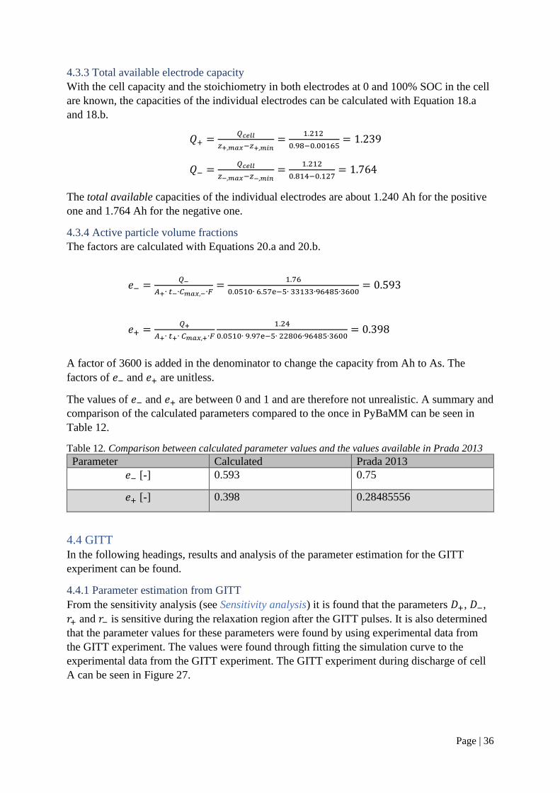
Page | 36
4.3.3 Total available electrode capacity
With the cell capacity and the stoichiometry in both electrodes at 0 and 100% SOC in the cell
are known, the capacities of the individual electrodes can be calculated with Equation 18.a
and 18.b.
𝑄+ =𝑄𝑐𝑒𝑙𝑙
𝑧+,𝑚𝑎𝑥−𝑧+,𝑚𝑖𝑛=
1.212
0.98−0.00165= .2 9
𝑄− =𝑄𝑐𝑒𝑙𝑙
𝑧−,𝑚𝑎𝑥−𝑧−,𝑚𝑖𝑛=
1.212
0.814−0.127= .76
The total available capacities of the individual electrodes are about 1.240 Ah for the positive
one and 1.764 Ah for the negative one.
4.3.4 Active particle volume fractions
The factors are calculated with Equations 20.a and 20.b.
𝑒− =𝑄−
𝐴+∙ 𝑡−∙𝐶𝑚𝑎𝑥,−∙𝐹=
1.76
0.0510∙ 6.57e−5∙ 33133∙96485∙3600= 0. 9
𝑒+ =𝑄+
𝐴+∙ 𝑡+∙ 𝐶𝑚𝑎𝑥,+∙𝐹
1.24
0.0510∙ 9.97e−5∙ 22806∙96485∙3600= 0. 98
A factor of 3600 is added in the denominator to change the capacity from Ah to As. The
factors of 𝑒− and 𝑒+ are unitless.
The values of 𝑒− and 𝑒+ are between 0 and 1 and are therefore not unrealistic. A summary and
comparison of the calculated parameters compared to the once in PyBaMM can be seen in
Table 12.
Table 12. Comparison between calculated parameter values and the values available in Prada 2013
Parameter Calculated Prada 2013
𝑒− [-] 0.593 0.75
𝑒+ [-] 0.398 0.28485556
4.4 GITT
In the following headings, results and analysis of the parameter estimation for the GITT
experiment can be found.
4.4.1 Parameter estimation from GITT
From the sensitivity analysis (see Sensitivity analysis) it is found that the parameters 𝐷+, 𝐷−,
𝑟+ and 𝑟− is sensitive during the relaxation region after the GITT pulses. It is also determined
that the parameter values for these parameters were found by using experimental data from
the GITT experiment. The values were found through fitting the simulation curve to the
experimental data from the GITT experiment. The GITT experiment during discharge of cell
A can be seen in Figure 27.

Page | 37
Figure 27, GITT during discharge
In Figure 27, ten C/20 pulses (smaller voltage drop) and ten C/3 pulses (larger voltage drop)
can be seen in an alternating manner from the fully charged cell until the 2.0 V cut-off voltage
is triggered. The smaller C/20 pulses are the GITT pulses and the larger C/3 pulses moves the
cell into another SOC. In order to find optimal values for the parameters 𝐷+, 𝐷−, 𝑅+ and 𝑅−
each C/20 pulse is individually fitted to the experimental data using scipy.optimix.curve_fit.
The bounds for the parameters can be seen in Table 13.
Table 13. Bounds for curve fitting procedure of GITT.
Parameter Unit Prada 2013 value Lower bound Upper bound
𝐷+ 𝑚2
𝑠⁄ 5.9e-18 5.9e-19 5.9e-17
𝐷− 𝑚2
𝑠⁄ 3.3e-14 3.3e-15* 3.3e-13*
𝑅+ m 1e-08 1e-09 1e-07
𝑅− m 5.86e-6 5.86e-07 5.86e-05
*The bounds of the negative particle radius will be limited to 1e-6 – 1e-5 m in a second
iteration.
A selection of the plots from the curve fitting can be seen in Figure 28.

Page | 38
(a)
(b)
(c)
(d)
Figure 28, A selection of the fitted curves for four pulses. (a) shows the first C/20 pulse, (b) shows the eighth
pulse, (c) shows the ninth pulse and (d) shows the tenth pulse. The fitted curves of the rest of the pulses can be
found in Appendix C.
As explained in Sensitivity analysis for GITT, the region when the curve relaxes back to
equilibrium after the pulse is the most interesting feature to fit for GITT. From Figure 29, (a)
shows a fit that does not capture the relaxation relatively well. Both the simulation with the
Prada 2013 and the optimized values has a sharp appearance in the region where the
experimental data shows the relaxation. With these values it seems like the simulated
response relaxes and reaches equilibrium conditions much faster relative to the experimental
data shows. For most of the pulses (nr 1-7) the simulation does not capture the gradual
relaxation in a realistic way. See the fit for all the pulses in Appendix C. For the eighth, ninth
and tenth pulses the fit can be seen in Figure 29 (b), (c) and (d). The optimized values found
for these pulses give a better fit than the Prada 2013 values and yield the gradual relaxation
from the experimental data in a more realistic way than the other pulses. Figure 29 (b) shows
some disturbance in the experimental data, which is also included in the curve optimization
procedure. An observation from Figure 29 is that the simulated curves have higher voltages
than the experimental data, (b) and (d), and sometimes lower, (a) and (c). The values found
through the fitting procedure for the selected pulses as well as the values available in the
Prada 2013 parameter set can be seen in Table 14.

Page | 39
Table 14. Parameter values found via curve fitting for each GITT pulse
Origin of
values 𝐷+ [𝑚
2
𝑠⁄ ] 𝐷− [𝑚2
𝑠⁄ ] 𝑅+ [𝑚] 𝑅− [𝑚]
Bounds 5.9e-19 − 5.9e-17 3.3e-15 – 3.3e-13 1e-9 – 1e-7 5.86e-7 – 5.86e-5
Prada 2013 5.9e-18 3.3e-14 1e-8 5.86e-6
Pulse 1 2.895e-18 3.317e-14 4.650e-8 6.608e-06
Pulse 8 5.900e-17 3.300e-15 1.000e-9 2.390e-05
Pulse 9 5.219e-17 1.716e-14 4.988e-8 2.195e-05
Pulse 10 5.770e-17 1.104e-14 1.016e-9 3.102e-05
Mean* 2.77e-17 4.95e-14 3.37e-08 1.66e-05
STDEV* 2.62e-17 7.12959e-14 2.97e-08 8.84e-06
* The mean value and the standard deviation are based on the values found for all the fitted
pulses. See the fitted values for all the pulses in Appendix C.
From Table 14, it shows that the pulses nr 8, 9 and 10 (whose parameter values made the
simulation match the gradual relaxation of the experimental data) goes towards the upper
boundary for 𝐷+, especially for pulse nr 8. The electrochemical implication of this would be
that the diffusion goes faster at the positive electrode than the Prada 2013 values would give.
𝐷− lays within the middle of the boundary except for pulse nr 8 who matches the lower
bound. This would mean that the diffusion is slower at the negative electrode. The diffusivity
in the negative electrode is however still larger than in the positive electrode. The 𝑅+ goes to
the lower boundary value while the 𝑅− goes to the higher value. The particle radiuses are
affected by the production process.
To see how the parameter values found for pulse 8, 9 and 10 would impact the simulation for
the full discharge, Figure 29 is made. All ten pulses are not able to simulate because the lower
cut-of voltage is triggered by the ninth C/3 pulse.
Figure 29, GITT experiment during discharge. The blue curve represents the experimental data, the red is the
simulation with optimal parameters for pulse 8, the black is for pulse 9 and green is for pulse 10.
From Figure 29, it seems like the simulated relaxation is less visible in the region around
75000 - 125000 seconds while the slopes are more visible in the other pulses. The parameter
values are found by fitting the simulation to the C/20 pulses. Although, since the GITT

Page | 40
experiment has both C/20 and C/3 pulses Figure 30 is created by zooming in on two different
pulses to see the impact on fit that the C-rate gives.
(a)
(b)
Figure 30, Zoom in on Figure 29 on (a) a C/20 pulse, and (b) a C/3 pulse.
From Figure 30 it seems like the simulated values from pulse 8 and 10 matches the gradual
relaxation of the experimental data the best. For the C/20 pulse it looks like the values from
pulse 8 has the best match. From Figure 30 the simulations do not have as smooth appearance
as the experimental data. This is likely due to the numerical calculations that takes place in the
simulation where the solver fits a polynomial to the experimental data. The parameters that
best capture the relaxation time can be seen in the Table 15 below.
Table 15. The parameter values of the best fitted pulse (8) compared to Prada 2013 parameter set
Parameter Unit Value Prada 2013
𝐷+ 𝑚2
𝑠⁄ 5.900e-17 3.3*10^-14
𝐷− 𝑚2
𝑠⁄ 3.300e-15 3.3*10^-14
𝑟+ m 1.000e-09 1.00*10^-8
𝑟− m 2.390e-05 5.86*10^-6
Another run when the bound of the relatively sensitive parameter 𝑟− is limited in a tighter
manner, 1e-6 < 𝑟− < 1e-5, can be found in Appendix D.
4.4.2 Experiment analysis for GITT
From Figure 29 and 30, a voltage gap can be seen after each pulse where the experimental
data often has a higher voltage than the simulated curves. To visualize this better, the Figure
31 below shows the experimental data and the simulation with optimized parameters from
pulse 9 for the discharge involving nine C/20 pulses and eight C/3 pulses.

Page | 41
Figure 31, the voltage offset between the experimental data and the simulated data for the GITT experiment.
The simulated curve operates as a lower voltage than the experimental data. The size of the
voltage gap differs in size throughout the experiment. This difference in voltage is not closely
related to the concentration overpotential but once again a result of the OCV curve found
from the low-rate cycling experiment. With correct OCV curves, the simulated pulses would
relax to the same place as the experimental data. It can also depend on that the cell is not fully
relaxed, at equilibrium, in the beginning of the GITT pulse.
In the GITT experiment, pulses with C/20 and C/3 are alternated. The C/3 pulses are used to
shorten the time for the experiment but also to get data from different SO levels by “fast
forwarding” to the next level. Four hours of rest is used between the C/3 and C/20 pulses to
give the cell time to go back to equilibrium conditions. The new pulse should start at
relaxation, which might not always be correct as can be seen in the experimental data in
Figure 32.

Page | 42
Figure 32, Unfinished relaxation before GITT pulse.
In Figure 32 the voltage is not completely flat but that there is a slope in the mV range taking
place before the next pulse starts. This could mean that there is still relaxation taking place
from the last pulse that influence the appearance of the next one.
When the cell is at equilibrium, the voltage points should be present on the OCV-curve. The
voltage gap when the simulation is getting close equilibrium conditions, seen in Figure 31, is
although still relatively large in the order of around 20-30 mV. This could be the result of the
OCV curve fit that might have resulted in errors in the stoichiometric ratios for the electrodes,
individual electrode capacity etc.
4.5 Pulse test
In the following headings, results and analysis of the parameter estimation for the Pulse test
can be found.
4.5.1 Parameter estimation from Pulse test
From the sensitivity analysis (see Sensitivity analysis) it is determined that the values of the
𝑘𝑓− is going to be found from the pulse test. The bounds are 0.5 < 𝑘𝑓− < 5. The pulse test
experiment during discharge can be seen in Figure 33.

Page | 43
Figure 33, Pulse test during discharge
In Figure 33, there are ten pulse trains consisting of four ten-seconds pulses in each with a
five-minute rest in between (see Experiment methods for more experimental details). It is
decided that only the C/2 pulse in each pulse train was utilized for fitting the values due to
time restrictions. A selection of the plots from the curve fitting can be seen in Figure 34.
(a)
(b)

Page | 44
(c)
(d)
Figure 34, the plots when only kf- is fitted. (a) pulse 2, (b) pulse 5, (c) pulse 8 and (d) pulse 9.
As explained in Sensitivity analysis for the pulse test, the depth of the pulse is the most
interesting feature to fit. From Figure 34, (a) shows a plot where the fitted kf- value give a
relatively large improvement compared to the simulation with the default value. The
simulation with the default value has a larger voltage drop compared to the experimental data.
By comparing (a), (b), (c) and (d) it appears that the simulation with the default kf- value fit
the experimental data better at lower SOC levels (higher pulse number). While the simulation
using the default value fits the experimental data better for pulse 8 and 9, the simulation with
the fitted kf- is lower than 0.01 V off compared to the experimental data in all the plots. By
favouring the simulation that had a better match to the experimental data than the simulation
with the default value, the parameter values of pulse 2 is considered the most suitable fit. It
could be argued that the default value could also be of interest for lower SOC levels. The
values found through the fitting procedure for the selected pulses as well as the values
available in the Prada 2013 parameter set can be seen in Table 16.
Table 16. The fitted parameter values from the simulation
Origin of
values 𝑘𝑓− [-]
Bounds 0.5 − 5
Prada 2012 1
Opt. Train 2 2.26116222
Opt. Train 5 1.65668429
Opt. Train 8 1.38499424
Opt. Train 9 1.31931518
Mean* 1.746649983
SDEV* 0.330851661
* The mean value and the standard deviation are based on the values found for all the fitted
pulses. See the fitted values for all the pulses in Appendix C.
From Table 16, it shows that the values of 𝑘𝑓− is in the lower part of the bound. As the pulses
are found in the lower part of the SOC window, the 𝑘𝑓− value becomes closer to the default
value.

Page | 45
4.5.2 Experiment analysis for Pulse test
In order to follow up on the sensitivity analysis for the pulse test, the parameters 𝑘𝑓−, 𝑘𝑓+, 𝜎−
and 𝜎+ are fitted one-by-one to see the effect on the simulation. The bounds used can be seen
in Table 17.
Table 17. Bounds for parameters used in the experimental analysis for the Pulse test.
Parameter Unit Prada 2013 value Lower bound Upper bound
𝑘𝑓− - 1 0.5 5
𝑘𝑓+ - 1 0.5 5
𝜎− 𝑆𝑚⁄ 215 190 250
𝜎+ 𝑆𝑚⁄ 0.338 0 0.5
Figure 35 show the fitted simulations together.
(a)
(b)
Figure 35. Fitting one parameter at the time. (a) shows a pulse with all simulations. (b) show a zoom in on the lower part of
the pulse in (a).
Figure 35 confirms the sensitivity analysis because the simulations where the optimal values
for the electrode conductivities are placed precisely on top of the simulation with the default
values from the Prada 2013 parameter set. The simulation with the optimal value for the
factor 𝑘𝑓+ shows a small change compared to the default values, but not in the same range as
the 𝑘𝑓−does.

Page | 46
4.6 Validation
The fitted values of the parameters can be seen in Table 18.
Table 18. Estimated parameter values found from parametrization
Parameter Unit New value Prada 2013 value
Negative electrode thickness m 6.57e-5 3.6e-5
Positive electrode thickness m 9.970e-5 8.1e-5
Electrode height m 5.7e-2 0.0649
Electrode width m 0.895 1.78
Negative current collector thickness m 1.633e-5 1e-5
Positive current collector thickness m 1.933e-5 1.9e-5
Separator thickness m 1.6e-5 1.8e-5
Positive electrode active material volume
fraction
- 0.399 0.285
Negative electrode active material volume
fraction
- 0.593 0.75
Positive electrode diffusivity 𝑚2
𝑠⁄ 5.9e-17 5.9e-18
Negative electrode diffusivity 𝑚2
𝑠⁄ 3.3e-15 3.3e-14
Positive particle radius m 1e-09 1e-8
Negative particle radius m 2.39e-05 5.86e-6
Reaction rate factor 𝑘𝑓− - 1.747 1
Reaction rate factor 𝑘𝑓+ - Unchanged 1
Positive electrode conductivity 𝑆𝑚⁄ Unchanged 0.33795074
Negative electrode conductivity 𝑆𝑚⁄ Unchanged 215.0
The parameter values were used in two different scenarios to validate in a qualitative manner
to evaluate the simulation matches experimental data. For both validation scenarios, the cell
capacity will have a large impact on how well the simulation matches the experimental data.
4.6.1 BEV application
The found parameter values were used to simulate a possible BEV application and is then
compared to experimental data. The block diagram for the BEV application can be found in
Figure 36.
Figure 36, Potential BEV application block diagram
When trying to use the found value for the negative particle radius, the CasADI solver in
PyBaMM fails due to exceed interpolation bounds. A trial is done by using the parameter
values from the ninth and tenth GITT pulse, where the relaxation time is also reasonable, but

Page | 47
the same error message appeared. To be able to plot the simulation, the default value for the
negative particle size is used instead of the fitted value.
The experimental data of the BEV application is compared with two simulations. One where
only the thermodynamic values are changed from the default values and another where all the
found parameter values are used (except for the negative particle radius where the default is
used). See Figure 37 for the plots.
(a)
(b)
(c)
Figure 37, (a) shows the BEV application experimental data compared to a simulation with the thermodynamic
values changed from default, (b) shows the same as (a) but when the simulation includes changed values for all
the found parameters except for r- which is default. (c) is a zoom in on the constant voltage and rest region in
(a). The red curve is the experimental data, and the blue curve is the simulation.
From the Figure 37 (a) the full run can be seen. As Figure 37 (b) shows, the simulation has a
longer resting phase between about 3000-10500 s compared to the experimental data where
the phase is only between around 3500-4000 s. The flat part of the red curve is the constant
voltage step that moves on to the next part of the sequence when limit |I|< 0.55 A is triggered
or after 1 hour. The slope following the flat part of the red curve represents the 1-hour rest
period when the cell relaxes to around 3.37 V. After that hour it can be seen that the slope is
not flat and that the cell has not reached equilibrium yet. The experimental data and the

Page | 48
simulation indicate that the |I|-limit is triggered before the 1 hour had passed. In the
simulation, this limit is triggered earlier and that the cell relaxes in a fast manner to around
3.56 V for the rest.
By moving in the simulated SO window and plotting the experiment starting from the “ est
for minute”-segment Figure 38 is made for the shortened experiment. The non-equilibrium
state of the cell that exists in the experimental data before the segment is a bit difficult to
account for in the simulation and will cause some difference between the graphs.
Figure 38, BEV application. The simulation with the found parameter values and with the negative particle
radius value set to default.
From Figure 38 the simulation has similar curvature as the experimental data. The simulated
curve matches the experimental data relatively well for the discharge parts of the run until
around 17500 s, but that the voltage gap increases significantly as the cell is charged. At the
endpoint, the voltage difference is clearly seen. It is unexpected since the same current is used
which would result in a similar change in capacity and that the cell starts at the same voltage.
This might be a result of that the cell is not at relaxed state in the start of these segment. The
cell could continue to relax in the red curve which would give the endpoints different values.
This could be tested by performing the test once again but letting the cell rest for more than 1
hour to reach equilibrium before starting the potential BEV application activities. Another
theory is that the cell capacity is different in the experiment and simulation which would be
the result of errors in the OCV-curve fitting and the found vales for the active particle fraction
in the electrodes. A third theory to why there is a voltage in the end of the simulation is that
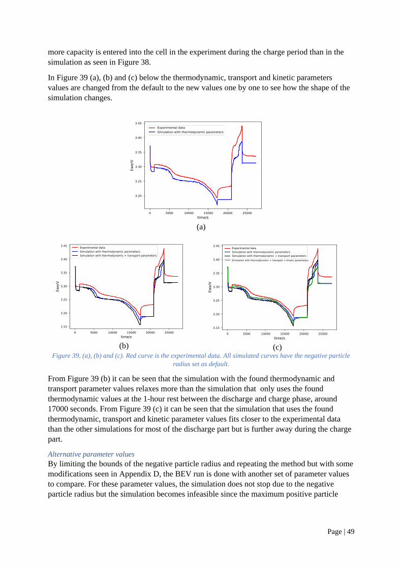
Page | 49
more capacity is entered into the cell in the experiment during the charge period than in the
simulation as seen in Figure 38.
In Figure 39 (a), (b) and (c) below the thermodynamic, transport and kinetic parameters
values are changed from the default to the new values one by one to see how the shape of the
simulation changes.
(a)
(b)
(c)
Figure 39, (a), (b) and (c). Red curve is the experimental data. All simulated curves have the negative particle
radius set as default.
From Figure 39 (b) it can be seen that the simulation with the found thermodynamic and
transport parameter values relaxes more than the simulation that only uses the found
thermodynamic values at the 1-hour rest between the discharge and charge phase, around
17000 seconds. From Figure 39 (c) it can be seen that the simulation that uses the found
thermodynamic, transport and kinetic parameter values fits closer to the experimental data
than the other simulations for most of the discharge part but is further away during the charge
part.
Alternative parameter values
By limiting the bounds of the negative particle radius and repeating the method but with some
modifications seen in Appendix D, the BEV run is done with another set of parameter values
to compare. For these parameter values, the simulation does not stop due to the negative
particle radius but the simulation becomes infeasible since the maximum positive particle
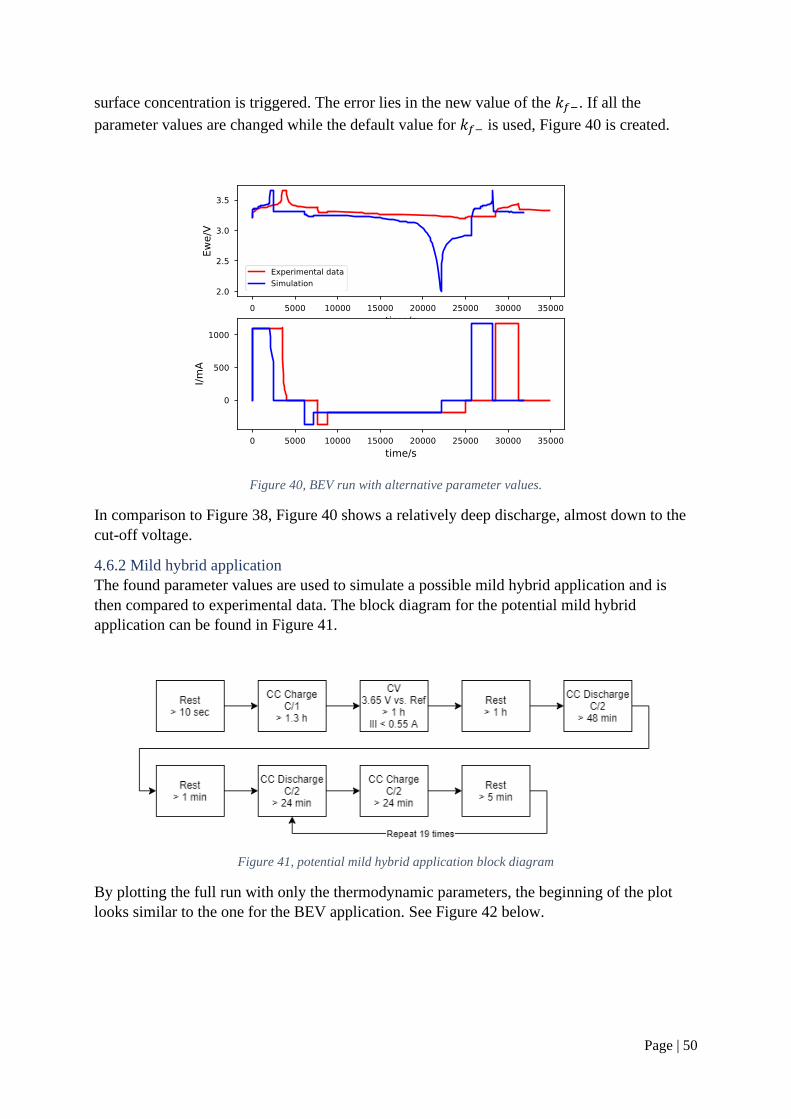
Page | 50
surface concentration is triggered. The error lies in the new value of the 𝑘𝑓−. If all the
parameter values are changed while the default value for 𝑘𝑓− is used, Figure 40 is created.
Figure 40, BEV run with alternative parameter values.
In comparison to Figure 38, Figure 40 shows a relatively deep discharge, almost down to the
cut-off voltage.
4.6.2 Mild hybrid application
The found parameter values are used to simulate a possible mild hybrid application and is
then compared to experimental data. The block diagram for the potential mild hybrid
application can be found in Figure 41.
Figure 41, potential mild hybrid application block diagram
By plotting the full run with only the thermodynamic parameters, the beginning of the plot
looks similar to the one for the BEV application. See Figure 42 below.

Page | 51
(a)
(b)
Figure 42, full Mild hybrid run (a) with only thermodynamic values changed (b) with all new values except for
the negative particle radius.
Since the negative particle radius causes the simulation to stop in the potential BEV
application, a simulation with the default value of that parameter can be seen in Figure 43
while the other found parameter values are used.
Figure 43, Potential mild hybrid application with the red curve representing experimental data and the blue
curve the simulation with the found parameter values except for negative particle radius.
Figure 43 shows a better match between the simulation and experimental data, although the
simulation does not reach the experimental end points of each charge and discharge phase.
The experimental data moves higher up in voltage for each charging phase while the
simulation reaches about the same voltage level.
In Figure 44 below, the difference from adding a set (thermodynamic, transport and kinetic
parameters) of found parameter values can be seen. Figure 44.a shows the experimental data

Page | 52
and the simulation where the thermodynamic parameter values has been changed from the
default. Figure 44.b shows the difference in appearance when the other parameter sets are
used in the simulation.
(a)
(b)
(c)
(d)
Figure 44. a, b, c, d. All simulated curves have the negative particle radius excluded.
Figure 44.c and 44.d it seems like the simulation comes closer to the end points of charge and
discharge pulses of the experimental data when the kinetic parameter is not included. The
voltage at the end of discharge is reached with only the thermodynamic parameters but the
transport parameters make the relaxation more similar the experimental data. The simulation
with all parameters except for the negative particle radius influences which voltage the
simulation reaches after charge and discharge.
Alternative parameter values
Just as for the BEV application, the alternative parameter set found by limiting the bounds of
the negative particle radius and repeating the method just as but with some modifications seen
in Appendix D, the mild hybrid run will also be investigated. If all the parameter values are
changed to the alternative parameter values while the default value for 𝑘𝑓− is used, Figure 45
is created.

Page | 53
Figure 45, Mild hybrid run with alternative parameter values
In comparison to Figure 43, Figure 45 has a rather similar appearance.
5. DISCUSSION From the sensitivity analysis, to disturb the parameters by ±10 % might be an unrealistic
disturbance if the parameters values would pass outside of a physical boundary. An
alternative method is to find within which ranges the parameters are usually found and then
disturb the parameters within that range. The risk of using the simpler method is assumed to
be acceptable in order to get a quick and simple overview of the parameter’s sensitivity.
From the sensitivity analysis, it seems like the electrode conductivities are not sensitive to the
small changes of ± 10 % in the parameter values. This is an unexpected result since the
conductivity is related to the resistance in the cell which would give linear dependence
according to Ohms law. The lowest conductivity in the LFP electrode should reasonably limit
the reaction rate more than the graphite electrode, although no difference is found. The effect
is looked at in the Sensitivity analysis and in the Mild hybrid application and they gave
similar outputs. The exchange current density for the LFP is lower than for graphite. From the
Butler-Volmer equation, the largest exchange current density has the largest impact. It might
be that the effect from the changed reaction rate for the LFP cannot be seen after 10 seconds
and that the effect is visible first after a longer rest. This might also be something that the
SPM does not capture.
The cell´s geometric parameters were measured in a reasonable accurate way to values that
are comparable to the Prada 2013 parameter values. Even more points could have been used
to measure the thickness of the current collector.
From the low-rate cycling curve fitting seen in Figure 26, the fitted simulation curve has a
higher voltage at 100 % SOC compared to the experimental data. This error could lead to

Page | 54
unrealistic voltage values when the cell is working on high SOC levels. The OCV-curve is
weighted extra to the graphite bumps in the middle of the SOC window while the endpoints
are weighted less. In real applications, the full SOC window of the battery cell is rarely used
because the risk is higher for irreversible side reaction, shorter lifetime etc. The LFP/C has a
rather flat OCV curve and the change in voltage is concentrated at the higher SOC value. By
operating up to around 83% SOC, the simulation fits reasonably well to the experimental data.
The stochiometric values within the electrodes are found through the OCV-curve fitting. For
the LFP electrode these values are between 0.001-0.98 which would mean that a very large
part of the SOC window of the LFP electrode is also used in the cell. This is a large usage of
the LFP´s SOC window since the maximum range was 0-1. The method used gave these
values but maybe another could be used to compare and validate the values. During
conversation with Alexander Bessman and Pontus Svens, these ranges seem realistic.
Since thermodynamic parameters (geometric and found through the low-rate cycling test) are
set before the transport and kinetic parameters are found, an error in them would cause errors
in the other parameter values as well. The thickness of the geometrical parameters were
measured in micrometers, and is sensitive to errors. When the electrode coating was scarpaed
of, eyesight was used to determine when the surface was free of coating. Small rest pieces that
were not visible with the eye might still be present on the surface which generate an error in
the measurement.
In Table 9, there is a small difference between the charge and discharge capacity. It is
expected that the charge capacity would be smaller than the discharge capacity due to
irreversible side reactions. When the cell was cycled at C/50, this was seen. For the
experimental tests, it would be good to make sure that the cell is at equilibrium condition
before the comparison or fitting procedure begins. The risk is otherwise that possible
relaxation from a previous activity on the cell can disturb and make it difficult to use as has
been seen in the thesis.
In relation to Figure 37, the lack of relaxation in the simulation is likely due to errors in the
OCV-curve from the low-rate cycling experiment. The OCV-curve is fitted with weights
around the graphite “bumps” in the middle of the curve while the endpoints, when the cell is
or is near fully charged or discharged, is weighted less to promote the fit of the bumps. This
could be a reason why equilibrium points in the simulation does not fit the experimental data
very well compared to other parts of the curve.
In relation to Figure 37. This difference could be a result of that all the parameter values has
been found and fitted to experimental data when the cell is discharged. This is a weakness in
the method that could be investigated in future work. Physically, the found parameters should
be the same for charge and discharge but because of this validation, it seems reasonable to
question if that is really the case. It might have been better to find mean values for the found
and fitted parameters for both charge and discharge.
From the BEV application validation, the negative particle radius hit the upper bound in
PyBaMM which stopped the simulation. This means that the parametrization is not optimal
for this parameter and that the bounds are set too freely. The interpolation ranges within the
literature that PyBaMM bases its values on could not work with the parameter value. From
the mild hybrid application validation, it is seen that the negative particle radius affected the

Page | 55
fit in an unwanted way and gave unrealistic results. This is a further indicator that the
parametrisation of the negative particle radius is not effective. A solution to this would be to
limit the bounds more. The bounds for the negative particle radius were limited more, and an
alternative method where the values from both the cell opening, low-rate cycling and GITT
are used before the values of the factor to the negative electrodes reaction rate is found. The
negative particle radius and reaction rate seem to be tightly connected when they aim to be
fitted to the GITT or pulse test. When the bounds are less restricted, the negative particle
radius finds its optimal value above the interpolation limit during the BEV run while the
factor of the negative reaction rate stays in the middle of the bounds. The negative electrode
radius bounds are limited, the factor to the negative electrodes reaction rate hits goes to the
upper bound value and makes the BEV run unfeasible. A theory is that there are some other
phenomenon taking place that is related to the negative particle radius and the negative
electrode reaction rate that the adapted parameters does not capture. There can be some other
unknown parameter that better represents the phenomena.
For the mild hybrid validation run, a theory why the experimental data and simulation look
different from charge and discharge is related to the voltage level used. Around 3.3 V is the
position of a graphite “bump” in the O curve which can be seen in Background.
The negative particle radius is shown to be relatively sensitive for both the GITT and the
pulse test. The initial procedure is to find the parameter values from GITT and Pulse test
when using the default and thermodynamic values. An alternative method when the parameter
for the Pulse test is found when using both the default, thermodynamic and transport
parameters is also tested. From both the procedures, it seems like the values for negative
particle radius and negative electrode reaction rate are not successfully found. A conclusion
can be made that the negative particle radius cannot be estimated accurately with this method.
From the BEV and Mild hybrid validation runs, the simulation appeared to fit better during
discharge than charge. The physical parameter values should be the same for discharge and
charge. A way to investigate this could be to make the parametrization for the charge part of
the experiment, or to use data from both scenarios.
5.1 Future Work
For future work, the literature review could be extended in order to set even tighter bounds for
the curve fit procedure. The reasonability of changing the parameters by 10% or more within
the fitting procedure would also be relevant to investigate.
It would be interesting to fit even more parameters for every test to see which are sensitive for
different experiments. By finding which parameters that are sensitive under which conditions,
optimal tests could be formulated and tested to parameters experimentally. The particle radius
could for example be analysed through scanning electron microscope.
The OCV has a big impact on the simulations. In the pseudo OCV-fitting (see Results) the
experimental data, which the fitting is made on, is weighted to fit the graphite “bumps” in
order to capture the phenomena well. In order to get a satisfying fit over the bumps, a lower
weight is given to the endpoints of the experimental data. This gives a less accurate fit in the
simulation when being in high and low SOC-regions. In order to get more accurate OCV-
curves a GITT experiment with many more GITT pulses that maps up the equilibrium voltage

Page | 56
along the SOC window would be recommended. This is a time-consuming process that can
take months and is not included in this thesis but could be done in future work.
The value of the diffusivity in the solid can vary depending on the choice of method as
described in the Background. This makes it tricky to get an accurate value of the parameter. A
comparison could be done by conducting tests with other methods such as current pulse
relaxation, potential step chronoamperometry and AC impedance spectroscopy and compare
the values received from GITT. The parameters gotten from the other tests could be used as
parameter values in order to which value, and method, that is most suitable to use. This can be
a part of future work since it did not fit within the time frame of this thesis.
During the curve fitting procedure of the simulation to the experimental data, the pulses in the
end of the discharge, pulses eight, nine and ten with the low SOC levels, are the once that
showed the most relaxation and matched the experimental data the best. A future work could
be to investigate why the simulation showed that behaviour for these pulses and not for the
others.
The pulse test is related to the SOC but not to the current rate since only the C/2 pulses are
investigated due to time restrictions. The pulses with the lowest current rates are chosen to
look at because they had a longer relaxation time before them. The effect of current rates is
interesting to investigate in future work.
The long time needed for the cell to reach equilibrium conditions in the GITT test is likely
due to the flat OCV-curve of the LFP/C cell. By running the time consuming GITT test first
with 2-hour rest period and then the 4-hour rest took over half a month to conduct. A setting
on the instrument that could sense when the variation in voltage is acceptably small would
have been useful in this scenario. For future work, it would be recommended to be able to use
this setting when performing GITT tests on LFP/C cells to make sure that equilibrium
conditions are reached.
It would be interesting to investigate how parameters change due to degradation mechanisms
with PyBaMM simulations. This could be done in future work.
When a method of parametrization has been found to be successful, there are computational
problems that need to be solved in order to take the next step and use electrochemical battery
models instead of empirical models for applications like BMS. To tackle the computational
problems is a future work.
6. CONCLUSION The goals of the thesis were to parameterize the SPM from the open source PyBaMM
modelling library for commercial LFP cells. 17 parameters are investigated, and 14 parameter
values are adapted from the Prada 2013 parameter set. Another goal is to use literature survey
as well as experiments in the parametrization procedure. This took form as Table 2 as well as
the methods used. Three types of experimental tests are done to be able to estimate the
parameter values from the data. The third goal is to validate the model against drive cycles.
Two potential applications for a BEV and Mild hybrid are tested experimentally and used as
validation cycles.
The validation shows that this method and model cannot be used to find parameter values for
the negative particle radius.

Page | 57
Physics-based models have several advantages towards empirical models when it comes to
describing electrochemical systems. Parametrization is a time-consuming process but
necessary to make the model describe the system in an accurate way. A method to
parameterize a battery cell is complicated and more research is needed in the field.

Page | 58
7. REFERENCES [1] IPCC, 2014: Climate Change 2014: Synthesis Report. Contribution of Working Groups
I, II and III to the Fifth Assessment Report of the Intergovernmental Panel on Climate
Change [Core Writing Team, R.K. Pachauri and L.A. Meyer (eds.)]. IPCC, Geneva,
Switzerland, 151 pp. Avaliable: https://www.ipcc.ch/report/ar5/syr/
[2] Lindsey, Rebecca and Dahlman, LuAnn. Climate Change: Global Temperature.
NOAA Climate.gov. March 15, 2021. Accessed June 4, 2021. Avalaible:
https://www.climate.gov/news-features/understanding-climate/climate-change-global-
temperature
[3] Ritchie, Hannah. Sector by sector: where do global greenhouse gas emissions come
from?, Our world in data. September 18, 2020. Accessed on: April 5, 2021. Avaliable:
https://ourworldindata.org/ghg-emissions-by-sector
[4] Ritchie, Hannah and Roser, Max. CO₂ and Greenhouse Gas Emissions, Our world in
data. Published May 2017 and last revised August 2020. Accessed on: April 5, 2021.
Avaliable: https://ourworldindata.org/co2-and-other-greenhouse-gas-emissions
[5] Göran Lindbergh, “Class lecture, topic: Lecture 1 Electrochemcial energy devices
K 00”. Course: Electrochemical energy devices KE2300. Applied Electrochemistry,
Department of Chemical Engineering School of Engineering Sciences in Chemistry,
Biotechnology and Health, KTH - Royal Institute of Technology. N,” 0 9.
[6] A. Fotouhi, . J. Auger, K. Propp, S. Longo, and M. Wild, “A review on electric
vehicle battery modelling: From Lithium-ion toward Lithium-Sulphur,” Renewable and
Sustainable Energy Reviews, vol. 56. Elsevier Ltd, pp. 1008–1021, Apr. 01, 2016, doi:
10.1016/j.rser.2015.12.009.
[7] P. Svens, “ lass lecture, topic: ‘Lithium-ion batteries for electrified vehicles’, ourse:
Electrochemical energy devices KE2300. Applied Electrochemistry, Department of
Chemical Engineering School of Engineering Sciences in Chemistry, Biotechnology
and Health, KTH ,” 0 9.
[8] Dahn, Jeff and Ehrlich, "Lithium-ion batteries", Linden's handbook of batteries, 4th ed.
New York: McGraw-Hill, 2011. Chapter 26.
[9] W. hen, J. Liang, Z. Yang, and G. Li, “A review of lithium-ion battery for electric
vehicle applications and beyond,” in Energy Procedia, Feb. 2019, vol. 158, pp. 4363–
4368, doi: 10.1016/j.egypro.2019.01.783.
[10] A. M. Bizeray, J. Kim, S. R. Duncan, and . A. Howey, “Identifiability and Parameter
Estimation of the Single Particle Lithium-Ion Battery Model,” IEEE Transactions on
Control Systems Technology, pp. 1862–1877, Sep. 2019.
[11] 2020 PyBaMM Team. “PyBaMM.” Accessed Jun. 05, 2021. Avaliable at:
https://www.pybamm.org
[12] E. Prada, D. Di Domenico, Y. Creff, J. Bernard, V. Sauvant-Moynot, and F. Huet, “A
Simplified Electrochemical and Thermal Aging Model of LiFePO 4-Graphite Li-ion
Batteries: Power and apacity Fade Simulations,” J. Electrochem. Soc., vol. 160 (4),
pp. A616–A628, 2013, doi: 10.1149/2.053304jes.
[13] . Lindström Wreland, “ lass lecture, topic: ‘Battery II’, ourse: lectrochemical
energy devices KE2300. Applied Electrochemistry, Department of Chemical

Page | 59
Engineering School of Engineering Sciences in Chemistry, Biotechnology and Health,
KTH - oyal Institute of Technology. N,” 0 9.
[14] A. ornell, “ lass lecture, topic: ‘ ell voltage and electrode potential’, ourse:
Applied electrochemistry KE2110. Applied Electrochemistry, Department of Chemical
Engineering School of Engineering Sciences in Chemistry, Biotechnology and Health,
KTH - oyal institut,” 0 9.
[15] . Lindström Wreland, “ lass lecture, topic: ‘Battery I’, ourse: lectrochemical
energy devices KE2300. Applied Electrochemistry, Department of Chemical
Engineering School of Engineering Sciences in Chemistry, Biotechnology and Health,
KTH - oyal Institute of Technology. 5 No.”
[16] A. ornell, “ lass lecture, topic: ‘ lectrode kinetics’, ourse: Applied
electrochemistry KE2110. Applied Electrochemistry, Department of Chemical
Engineering School of Engineering Sciences in Chemistry, Biotechnology and Health,
KTH - oyal institute of technology.,” 0 9.
[17] Newman, John S, "Introduction 1", in Electrochemical engineering,second edition.
New Jersey, USA. Prentice Hall, 1991, The diffusion layer, section 1.5., 9 pp.
[18] A. K. Padhi, K. 5 Nanjundaswamy, and J. B. Goodenough, “Phospho-olivines as
Positive- lectrode Materials for echargeable Lithium Batteries,” 16. E. M. Genies S.
Picart, Synth. Met, vol. 144, no. 4, p. 16, 1997.
[19] J.-M. Tarascon and M. Armand, “Issues and challenges facing rechargeable lithium
batteries,” Nature, vol. 414, no. 6861, pp. 359–367, Nov. 2001, doi:
10.1038/35104644.
[20] A. . Huggins, “Insertion eaction lectrodes,” in Advanced Batteries, Boston, MA:
Springer US, 2009, pp. 101–122.
[21] A. Blidberg, “LFP-course,” May 18, 2021. Internal course at Scania CV.
[22] H. . Abruña, Y. Kiya, and J. . Henderson, “Batteries and electrochemical
capacitors,” Phys. Today, vol. 61, no. 12, pp. 43–47, 2008.
[23] N. Sharma and M. Wagemaker, “Lithium-Ion Batteries,” Springer, ham, 0 5, pp.
139–203.
[24] Ogumi Z., Inaba M. (2002) Carbon Anodes. In: van Schalkwijk W.A., Scrosati B. (eds)
Advances in Lithium-Ion Batteries. Springer, Boston, MA. https://doi-
org.focus.lib.kth.se/10.1007/0-306-47508-1_3
[25] . elmas, M. Maccario, L. roguennec, F. Le ras, and F. Weill, “Lithium
deintercalation in LiFePO4 nanoparticles via a domino-cascade model,” Nat. Mater.,
vol. 7, no. 8, pp. 665–671, Aug. 2008, doi: 10.1038/nmat2230.
[26] A. Barai et al., “A comparison of methodologies for the non-invasive characterisation
of commercial Li-ion cells,” Progress in Energy and Combustion Science, vol. 72.
Elsevier Ltd, pp. 1–31, May 01, 2019, doi: 10.1016/j.pecs.2019.01.001.
[27] M. A. anzer and M. Petzl, “Advancements in O Measurement and Analysis for
Lithium-Ion Batteries,” IEEE Trans. ENERGY Convers., vol. 28, no. 3, pp. 675–681,
Sep. 2013, Accessed: May 24, 2021. [Online]. Available: https://ieeexplore-ieee-
org.focus.lib.kth.se/stamp/stamp.jsp?tp=&arnumber=6517504.

Page | 60
[28] W. reyer, J. Jamnik, . Guhlke, . Huth, J. Moškon, and M. Gaberšček, “The
thermodynamic origin of hysteresis in insertion batteries,” Nat. Mater., vol. 9, no. 5,
pp. 448–453, May 2010, doi: 10.1038/nmat2730.
[29] . Srinivasan and J. Newman, “ xistence of Path-Dependence in the LiFePO[sub 4]
lectrode,” Electrochem. Solid-State Lett., vol. 9, no. 3, p. A110, 2006, doi:
10.1149/1.2159299.
[30] M. A. oscher and . U. Sauer, “ ynamic electric behavior and open-circuit-voltage
modeling of LiFePO4-based lithium ion secondary batteries,” J. Power Sources, vol.
196, no. 1, pp. 331–336, Jan. 2011, doi: 10.1016/j.jpowsour.2010.06.098.
[31] S. Lee, J. Kim, J. Lee, and B. H. ho, “State-of-charge and capacity estimation of
lithium-ion battery using a new open-circuit voltage versus state-of-charge,” J. Power
Sources, vol. 185, no. 2, pp. 1367–1373, Dec. 2008, doi:
10.1016/j.jpowsour.2008.08.103.
[32] J. Groot, “III TH SIS FO TH G OF LI NTIAT OF NGIN ING
State-of-Health Estimation of Li-ion Batteries: ycle Life Test Methods.”
[33] D. A. Howey et al., “Making a case for battery modelling,” Interface - Electrochem.
Soc., vol. 29, no. 4, pp. 32–33, 2020, Accessed: Jun. 05, 2021. [Online]. Available:
https://issuu.com/ecs1902/docs/2020-if-win.
[34] G. Alexander and H. Anton, “Parametrization Of A Simplified Physical Battery
Model,” Feb. 2019, pp. 215–220, doi: 10.3384/ecp19157215.
[35] W. Li et al., “Parameter sensitivity analysis of electrochemical model-based battery
management systems for lithium-ion batteries,” Appl. Energy, vol. 269, p. 115104, Jul.
2020, doi: 10.1016/j.apenergy.2020.115104.
[36] “ evelopment of xperimental Techniques for Parameterization of Multi-scale
Lithium-ion Battery Models,” 0 0, doi: 0. 9 9 5-7111/ab9050.
[37] S. G. Marquis, . Sulzer, . Timms, . P. Please, and S. J. hapman, “An asymptotic
derivation of a single particle model with electrolyte,” arXiv. arXiv, May 29, 2019, doi:
10.1149/2.0341915jes.
[38] M. oyle, T. F. Fuller, and J. Newman, “Modeling of Galvanostatic Charge and
ischarge of the Lithium Polymer Insertion ell,” J. Electrochem. Soc., vol. 140, no.
6, pp. 1526–1533, Jun. 1993, doi: 10.1149/1.2221597.
[39] . Namor, . Torregrossa, . herkaoui, and M. Paolone, “Parameter identification of
a lithium-ion cell single-particle model through non-invasive testing,” J. Energy
Storage, vol. 12, pp. 138–148, Aug. 2017, doi: 10.1016/j.est.2017.04.008.
[40] A. Raue et al., “Structural and practical identifiability analysis of partially observed
dynamical models by exploiting the profile likelihood,” Bioinformatics, vol. 25, no. 15,
pp. 1923–1929, Aug. 2009, doi: 10.1093/bioinformatics/btp358.
[41] N. Jin, . L. anilov, P. M. J. an den Hof, and M. . F. onkers, “Parameter
estimation of an electrochemistry-based lithium-ion battery model using a two-step
procedure and a parameter sensitivity analysis,” Int. J. Energy Res., vol. 42, no. 7, pp.
2417–2430, Jun. 2018, doi: 10.1002/er.4022.
[42] Lain, Brandon, and Kendrick, “ esign Strategies for High Power vs. High Energy

Page | 61
Lithium Ion ells,” Batteries, vol. 5, no. 4, p. 64, Oct. 2019, doi:
10.3390/batteries5040064.
[43] The PyBaMM Team. “Parameters Sets — PyBaMM 0.4.0 documentation.” Avaliable
at: https://pybamm.readthedocs.io/en/latest/source/parameters/parameter_sets.html.
Accessed Jun. 05, 2021.
[44] M. Farkhondeh and . elacourt, “Mathematical Modeling of ommercial LiFePO
Electrodes Based on Variable Solid-State iffusivity,” J. Electrochem. Soc., vol. 159,
no. 2, pp. A177–A192, Jan. 2011, doi: 10.1149/2.073202jes.
[45] T. . Ashwin, A. McGordon, and P. A. Jennings, “A mass transfer based variable
porosity model with particle radius change for a Lithium-ion battery,” Electrochim.
Acta, vol. 232, pp. 203–214, Apr. 2017, doi: 10.1016/j.electacta.2017.02.129.
[46] . Srinivasan and J. Newman, “ ischarge Model for the Lithium Iron-Phosphate
lectrode,” J. Electrochem. Soc., vol. 151, no. 10, p. A1517, Sep. 2004, doi:
10.1149/1.1785012.
[47] M. Park, X. Zhang, M. hung, G. B. Less, and A. M. Sastry, “A TI L IN PRESS A
review of conduction phenomena in Li-ion batteries,” J. Power Sources xxx, 2010, doi:
10.1016/j.jpowsour.2010.06.060.
[48] T. . Tran, J. H. Feikert, . W. Pekala, and K. Kinoshita, “ ate effect on lithium-ion
graphite electrode performance,” 99 .
[49] T. L. Kirk, . P. Please, and S. J. hapman, “Physical modelling of the slow voltage
relaxation phenomenon in lithium-ion batteries.”
[50] A. M. Bizeray, J.-H. Kim, S. . uncan, and . A. Howey, “Identifiability and
Parameter Estimation of the Single Particle Lithium-Ion Battery Model,” IEEE Trans.
Control Syst. Technol., vol. 27, no. 5, pp. 1862–1877, Sep. 2019, doi:
10.1109/TCST.2018.2838097.
[51] X. G. Yang and . Y. Wang, “Understanding the trilemma of fast charging, energy
density and cycle life of lithium-ion batteries,” J. Power Sources, vol. 402, pp. 489–
498, Oct. 2018, doi: 10.1016/j.jpowsour.2018.09.069.
[52] . Zhao, J. Liu, and F. Ma, “ athode Chemistries and Electrode Parameters Affecting
the Fast Charging Performance of Li-Ion Batteries,” J. Electrochem. Energy Convers.
Storage, vol. 17, no. 2, May 2020, doi: 10.1115/1.4045567.
[53] Askeland D.R. (1996) Ceramic Materials. In: The Science and Engineering of
Materials. Springer, Boston, MA. https://doi-org.focus.lib.kth.se/10.1007/978-1-4899-
2895-5_14
[54] Tran, T. , Feikert, J. H, Pekala, . W, and Kinoshita, K, “ ate effect on lithium-ion
graphite electrode performance,” Journal of applied electrochemistry, vol. 26, no. 11,
pp. 1161–1167, 1996, doi: 10.1007/BF00243741.
[55] Chang, Y.-C, Jong, J.-H, and Fey, G. T.-K, “Kinetic characterization of the
electrochemical intercalation of lithium ions into graphite electrodes,” Journal of the
Electrochemical Society, vol. 147, no. 6, pp. 2033–2038, 2000, doi:
10.1149/1.1393481.
[56] . Frackowiak and F. Béguin, “ arbon materials for the electrochemical storage of

Page | 62
energy in capacitors,” Carbon, vol. 39, no. 6. Elsevier Ltd, pp. 937–950, May 01, 2001,
doi: 10.1016/S0008-6223(00)00183-4.
[57] Z. Hui and L. Tao, “Lithium-ion Battery Series Product Specification Lithium-ion
Battery Series.” Available at: www.heter.biz.
[58] The SciPy community. “Scipy.optimize.curve_fit — SciPy v . . eference Guide.”
Avaliable at:
https://docs.scipy.org/doc/scipy/reference/generated/scipy.optimize.curve_fit.html.
Accessed June 5, 2021.
[59] M. ubarry and G. Baure, “Perspective on ommercial Li-ion Battery Testing, Best
Practices for Simple and ffective Protocols,” Electronics, vol. 9, no. 1, p. 152, Jan.
2020, doi: 10.3390/electronics9010152.
[60] A. Barai et al., “A comparison of methodologies for the non-invasive characterisation
of commercial Li-ion cells,” Prog. Energy Combust. Sci., vol. 72, pp. 1–31, May 2019,
doi: 10.1016/j.pecs.2019.01.001.
[61] Häggblom, Kurt-Erik. “5. Enkla dynamiska system.” Reglerteknik grundkurs. 2005.
Chapter 5. Accessed: Apr. 19, 2021. [Online]. Available at:
http://www.users.abo.fi/khaggblo/RTG/RTGk.pdf.

Page | 63
8. APPENDIX Appendix A – Parameter values in the Prada2013 parameter set
Table 19. Prada 2013 parameter values.
Parameter Value Unit Parameter Value Unit
1 +
dlnf/dlnc
1.0 - Ambient
temperature
298.15 K
Cation
transference
number
0.2594 - Cell capacity
1.1 Ah
Current
function
4.4 A Electrode height
0.0649 m
Electrode
width
1.78 m Electrolyte
conductivity
function
electrolyte_cond
uctivity_Nyman
2008 at
0x000002D24C
482D30
S.m-1
Electrolyte
diffusivity
function
electrolyte_diffusi
vity_Nyman2008
at
0x000002D24C4
82DC0
m2.s-1 Heat transfer
coefficient
10.0 W.m-
2.K-1
Initial
concentratio
n in
electrolyte
1200.0 mol.m-
3
Initial
concentration in
negative
electrode
28831.45783 mol.m-
3
Initial
concentratio
n in positive
electrode
35.3766672 mol.m-
3
Initial
temperature
298.15 K
Lower
voltage cut-
off
2.0 V Maximum
concentration in
negative
electrode
33133.0 mol.m-
3
Maximum
concentratio
n in positive
electrode
22806.0 mol.m-
3 Negative current
collector
conductivity
58411000.0 S.m-1
Negative
current
collector
density
8960.0 kg.m-3 Negative current
collector
specific heat
capacity
385.0 J.kg-
1.K-1
Negative
current
collector
401.0 W.m-
1.K-1
Negative current
collector
thickness
1e-05 m

Page | 64
thermal
conductivity
Negative
electrode
Bruggeman
coefficient
(electrode)
1.5 - Negative
electrode
Bruggeman
coefficient
(electrolyte)
1.5 -
Negative
electrode
OCP
entropic
change
0.0 V.K-1
Negative
electrode active
material volume
fraction
0.75 -
Negative
electrode
cation
signed
stoichiometr
y
-1.0 -
Negative
electrode charge
transfer
coefficient
0.5 -
Negative
electrode
conductivity
215.0 S.m-1 Negative
electrode
density
1657.0 kg.m-3
Negative
electrode
diffusivity
3.3e-14 m2.s-1 Negative
electrode
double-layer
capacity
0.2 F.m-2
Negative
electrode
electrons in
reaction
1.0 -
Negative
electrode
exchange-
current density
function
graphite_LGM5
0_electrolyte_ex
change_current_
density_Chen20
20 at
0x000002D24C
4073A0
A.m-2
Negative
electrode
porosity
0.25 - Negative
electrode
specific heat
capacity
700.0 J.kg-
1.K-1
Negative
electrode
thermal
conductivity
1.7 W.m-
1.K-1 Negative
electrode
thickness
3.6e-05 m
Negative
particle
radius
5.86e-06 m Negative tab
centre y-
coordinate
0.06 m
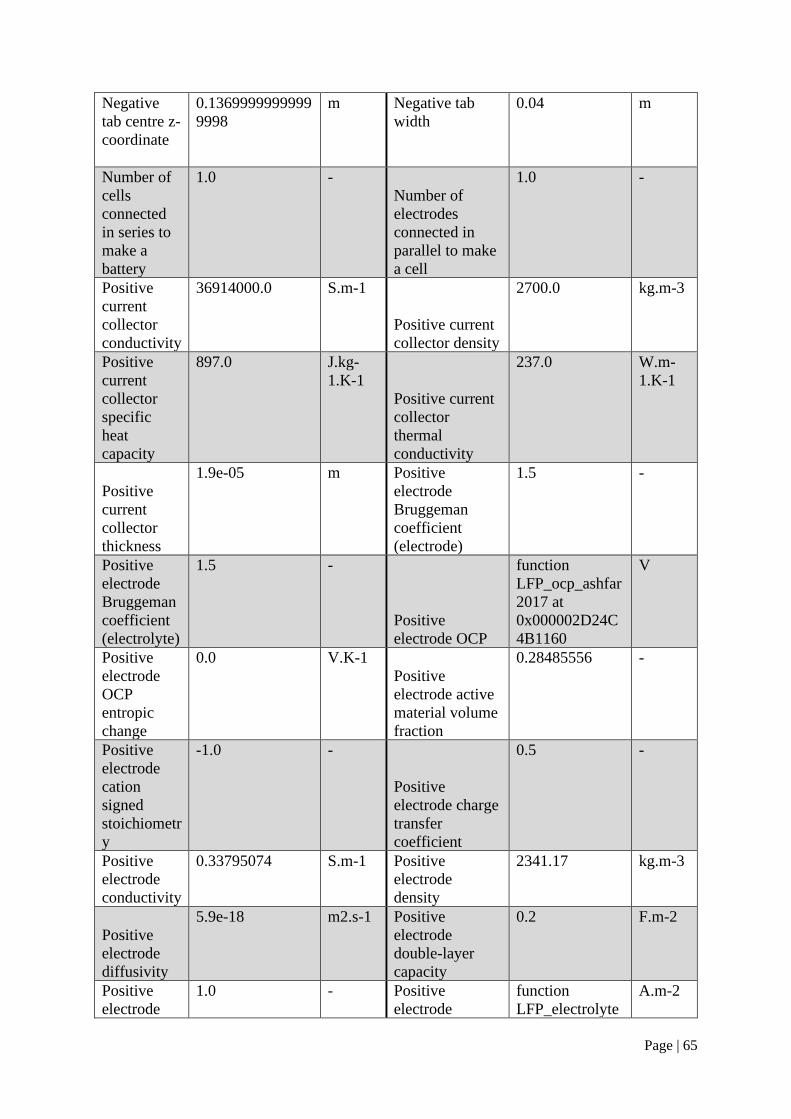
Page | 65
Negative
tab centre z-
coordinate
0.1369999999999
9998
m Negative tab
width
0.04 m
Number of
cells
connected
in series to
make a
battery
1.0 -
Number of
electrodes
connected in
parallel to make
a cell
1.0 -
Positive
current
collector
conductivity
36914000.0 S.m-1
Positive current
collector density
2700.0 kg.m-3
Positive
current
collector
specific
heat
capacity
897.0 J.kg-
1.K-1
Positive current
collector
thermal
conductivity
237.0 W.m-
1.K-1
Positive
current
collector
thickness
1.9e-05 m Positive
electrode
Bruggeman
coefficient
(electrode)
1.5 -
Positive
electrode
Bruggeman
coefficient
(electrolyte)
1.5 -
Positive
electrode OCP
function
LFP_ocp_ashfar
2017 at
0x000002D24C
4B1160
V
Positive
electrode
OCP
entropic
change
0.0 V.K-1
Positive
electrode active
material volume
fraction
0.28485556 -
Positive
electrode
cation
signed
stoichiometr
y
-1.0 -
Positive
electrode charge
transfer
coefficient
0.5 -
Positive
electrode
conductivity
0.33795074 S.m-1 Positive
electrode
density
2341.17 kg.m-3
Positive
electrode
diffusivity
5.9e-18 m2.s-1 Positive
electrode
double-layer
capacity
0.2 F.m-2
Positive
electrode
1.0 - Positive
electrode
function
LFP_electrolyte
A.m-2

Page | 66
electrons in
reaction
exchange-
current density
_exchange_curr
ent_density_kas
hkooli2017 at
0x000002D24C
4B10D0
Positive
electrode
porosity
0.12728395 - Positive
electrode
specific heat
capacity
1100.0 J.kg-
1.K-1
Positive
electrode
thermal
conductivity
2.1 W.m-
1.K-1 Positive
electrode
thickness
8.1e-05 m
Positive
particle
radius
1e-08 m Positive tab
centre y-
coordinate
0.147 m
Positive tab
centre z-
coordinate
0.1369999999999
9998
m
Positive tab
width
0.04 m
Reference
OCP vs
SHE in the
negative
electrode
nan V
Reference OCP
vs SHE in the
positive
electrode
nan V
Reference
temperature
298.15 K Separator
Bruggeman
coefficient
(electrode)
1.5 -
Separator
Bruggeman
coefficient
(electrolyte)
1.5 -
Separator
density
397.0 kg.m-3
Separator
porosity
0.47 - Separator
specific heat
capacity
700.0 J.kg-
1.K-1
Separator
thermal
conductivity
0.16 W.m-
1.K-1 Separator
thickness
1.8e-05 m
Typical
current
30.0 A Typical
electrolyte
concentration
1000.0 mol.m-
3
Upper
voltage cut-
off
4.4 V Negative
electrode OCP
graphite_LGM5
0_ocp_Chen202
0
V

Page | 67
Appendix B – Potential Mild hybrid application validation plots with the positive particle
radius
Figure 46, full run of mild hybrid potential application.
Just as for the potential BEV application plot, the constant voltage phase is ended since the |I|
limit is reached in the experimental data while not in the simulation. The simulation also
misses the relaxation during the one hour rest phase. In a similar way as the potential BEV
application, the potential mild hybrid application run will also be shorten in Figure 47.
Figure 47, Potential mild hybrid application. The blue curve the simulation with the found parameter values.

Page | 68
Figure 47 shows a bad match between the simulated and experimental data. For this
simulation PyBaMM did not stop the run because of interpolation issues as for the potential
BEV application. The simulated blue curve moves in a large voltage range than the
experimental data. In order to see each parameter types effect, Figure 48 is made.
(a)
(b)
(c)
Figure 48 a, b and c.

Page | 69
Appendix C – Curve fit plots for each pulse
GITT version 1
(a)
(b)
(c)
(d)
(e)
(f)

Page | 70
(g)
(h)
(i)
(j)
Figure 49, the experimental data, simulation with the Prada 2013 parameters as well as a simulation with fitted
parameter values for each of the ten GITT pulses. The order of the plots represents the order of the pulses in the
experiment.
Table 20. Parameter values found via curve fitting for each GITT pulse
Orgin of
values 𝐷+ [𝑚
2
𝑠⁄ ] 𝐷− [𝑚2
𝑠⁄ ] 𝑟+ [m] 𝑟− [m]
Prada 2013 5.9e-18 3.3e-14 1e-08 5.86e-06
Pulse 1 2.89e-18 3.32e-14 4.65e-08 6.61e-06
Pulse 2 2.78e-18 4.43e-15 4.70e-08 4.01e-06
Pulse 3 5.90e-17 1.73e-14 7.90e-09 8.02e-06
Pulse 4 5.90e-19 6.68e-14 9.99e-08 2.49e-05
Pulse 5 1.08e-17 2.42e-13 2.86e-08 1.39e-05
Pulse 6 2.60e-17 3.71e-14 2.35e-08 1.45e-05
Pulse 7 6.28e-18 6.31e-14 3.17e-08 1.72e-05
Pulse 8 5.90e-17 3.30e-15 1.00e-09 2.39e-05
Pulse 9 5.22e-17 1.72e-14 4.99e-08 2.20e-05
Pulse 10 5.77e-17 1.10e-14 1.02e-09 3.10e-05
Mean 2.77e-17 4.95e-14 3.37e-08 1.66e-05
STDEV 2.62e-17 7.13e-14 2.97e-08 8.84e-06

Page | 71
Pulse test version 1
(a)
(b)
(c)
(d)
(e)
(f)

Page | 72
(g)
(h)
Figure 50, the experimental data, simulation with the Prada 2013 parameters as well as a simulation with fitted
kf- for eight of the C/2 pulses. The order of the plots represents the order of the pulses in the experiment starting
with pulse nr 2.
Table 21. The fitted parameter values from the simulation
Orgin of values kf- [-]
PyBaMM 1
Opt. Train 2 2.26116222
Opt. Train 3 2.12878617
Opt. Train 4 1.96182209
Opt. Train 5 1.65668429
Opt. Train 6 1.81734881
Opt. Train 7 1.44308686
Opt. Train 8 1.38499424
Opt. Train 9 1.31931518
Mean 1.746649983
SDEV 0.330851661

Page | 73
Appendix D – Parametrization with changed r- bounds
Figure 51. Alternative parametrization process
By changing the bounds for the negative particle radius from 5.86e-7 - 5.86e-5 m to1e-6 – 1e-
5 m the results below are given.
GITT version 2
(a)
(b)

Page | 74
(c)
(d)
(e)
(f)
(g)
(h)

Page | 75
(i)
(j)
Figure 50, the experimental data, simulation with the Prada 2013 parameters as well as a simulation with fitted
parameter values for each of the ten GITT pulses. The order of the plots represents the order of the pulses in the
experiment.
Table 22. Parameter values found via curve fitting for each GITT pulse
Orgin of
values 𝐷+ [𝑚
2
𝑠⁄ ] 𝐷− [𝑚2
𝑠⁄ ] 𝑟+ [m] 𝑟− [m]
Prada 2013 5.9e-18 3.3e-14 1e-08 5.86e-06
Pulse 1 1.85e-18 3.30e-15 5.32e-08 6.44e-06
Pulse 2 7.32e-18 9.33e-15 4.64e-08 4.11e-06
Pulse 3 5.90e-17 3.30e-13 3.14e-08 7.81e-06
Pulse 4 5.90e-19 3.30e-15 9.99e-08 9.99e-06
Pulse 5 7.91e-19 1.42e-14 9.86e-08 9.92e-06
Pulse 6 6.27e-19 9.92e-15 9.56e-08 9.79e-06
Pulse 7 5.90e-19 3.30e-15 1.00e-07 1.00e-05
Pulse 8 5.90e-19 3.30e-15 1.00e-07 1.00e-05
Pulse 9 5.90e-19 3.30e-15 9.99e-08 9.99e-06
Pulse 10 9.50e-19 5.15e-15 9.90e-08 9.95e-06
Mean 7.29e-18 3.85e-14 8.24e-08 8.80e-06
STDEV 1.73e-17 9.72e-14 2.59e-08 1.94e-06
The simulation for the ninth pulse had the best fit to the experimental data.

Page | 76
Pulse test version 2
(a)
(b)
(c)
(d)
(e)
(f)

Page | 77
(g)
(h)
Table 23. The fitted parameter values from the simulation
Orgin of values kf- [-]
PyBaMM 1
Opt. Train 2 4.99
Opt. Train 3 4.99
Opt. Train 4 4.78
Opt. Train 5 3.41
Opt. Train 6 4.07
Opt. Train 7 3.02
Opt. Train 8 2.43
Opt. Train 9 2.56
Mean 3.78
SDEV 1.00
The simulation of the third pulse showed the best match with the experimental data.

Page | 78
BEV validation curve version 2
Figure 52, Stopped simulation for alternative parameter values
The simulation is stopped since the experiment was infeasible. The maximum positive particle
surface concentration' is triggered during 'Discharge at C/5.625 for 4.5 hours or until 2 V'.
The error lies in the 𝑘𝑓− value now. Before the bounds of 𝑟− is tightened this error message is
shown and the problem is related to the negative particle radius.

Page | 79
With kf- from pulse 6 instead
Figure 53, BEV simulation with alternative values except the k_f- is default.
Mild hybrid validation curve version 2
Figure 54. Mild hybrid run with alternative parameter values.


