Embed Size (px)
Citation preview

arX
iv:1
209.
0773
v2 [
gr-q
c] 2
2 O
ct 2
012
Perturbations of slowly rotating black holes:
massive vector fields in the Kerr metric
Paolo Pani,1, ∗ Vitor Cardoso,1, 2, † Leonardo Gualtieri,3, ‡ Emanuele Berti,2, 4, § and Akihiro Ishibashi5, 6, ¶
1CENTRA, Departamento de Fısica, Instituto Superior Tecnico,Universidade Tecnica de Lisboa - UTL, Av. Rovisco Pais 1, 1049 Lisboa, Portugal.
2Department of Physics and Astronomy, The University of Mississippi, University, MS 38677, USA.3Dipartimento di Fisica, Universita di Roma “La Sapienza” & Sezione INFN Roma1, P.A. Moro 5, 00185, Roma, Italy.
4California Institute of Technology, Pasadena, CA 91109, USA5Theory Center, Institute of Particle and Nuclear Studies,
High Energy Accelerator Research Organization (KEK), Tsukuba, 305-0801, Japan6Department of Physics, Kinki University, Higashi-Osaka 577-8502, Japan
We discuss a general method to study linear perturbations of slowly rotating black holes whichis valid for any perturbation field, and particularly advantageous when the field equations are notseparable. As an illustration of the method we investigate massive vector (Proca) perturbationsin the Kerr metric, which do not appear to be separable in the standard Teukolsky formalism.Working in a perturbative scheme, we discuss two important effects induced by rotation: a Zeeman-like shift of nonaxisymmetric quasinormal modes and bound states with different azimuthal numberm, and the coupling between axial and polar modes with different multipolar index ℓ. We explicitlycompute the perturbation equations up to second order in rotation, but in principle the method canbe extended to any order. Working at first order in rotation we show that polar and axial Procamodes can be computed by solving two decoupled sets of equations, and we derive a single masterequation describing axial perturbations of spin s = 0 and s = ±1. By extending the calculationto second order we can study the superradiant regime of Proca perturbations in a self-consistentway. For the first time we show that Proca fields around Kerr black holes exhibit a superradiantinstability, which is significantly stronger than for massive scalar fields. Because of this instability,astrophysical observations of spinning black holes provide the tightest upper limit on the mass ofthe photon: mγ . 4× 10⁻²⁰ eV under our most conservative assumptions. Spin measurements forthe largest black holes could reduce this bound to mγ . 10−22 eV or lower.
PACS numbers: 04.40.Dg, 04.62.+v, 95.30.Sf
I. INTRODUCTION
Linear perturbations of black holes (BHs) play a ma-jor role in physics. Many astrophysical processes can bemodeled as small deviations from analytically known BHbackgrounds: for instance, perturbative calculations ofquasinormal modes (QNMs) are useful to describe thelate stages of compact binary mergers or gravitationalcollapse [1–5], and BH perturbation theory provides anaccurate description of the general relativistic dynam-ics of extreme mass-ratio inspirals [6–8]. Even when theunderstanding of complex astrophysical phenomena re-quires numerical relativity, the set up of the numericalsimulations and the interpretation of the results are eas-ier when we can rely on prior perturbative knowledge ofthe problem (see e.g. [9, 10]).Besides their interest in modeling gravitational-wave
sources for present and future detectors in Einstein’s the-ory and in various proposed extensions of general relativ-ity, perturbative studies of BH dynamics are also relevant
∗ [email protected]† [email protected]‡ [email protected]§ [email protected]¶ [email protected]
in the context of high-energy physics [11]. Perturbationtheory can shed light on several open issues, such as thestability properties of BH spacetimes in higher dimen-sions and in asymptotically anti-de Sitter spacetimes.Within the gauge-gravity duality, some of the correla-tion functions and transport coefficients are related tothe lowest order BH QNMs. In a semiclassical treatmentof BH evaporation, the calculation of greybody factors(which may be of direct interest for ongoing experiments)relies heavily on our ability to understand wave scatter-ing in rotating BH spacetimes.
BH perturbation theory is a useful tool to investi-gate issues in astrophysics and high-energy physics aslong as the radial and angular parts of the perturbationequations are separable. This usually happens when thebackground spacetime has special symmetries. If sep-arable, the perturbation equations in the frequency do-main reduce to a system of ordinary differential equations(ODEs) [12]. Separability is the norm if the backgroundspacetime is spherically symmetric. Teukolsky [13] dis-covered that a large class of perturbation equations is ex-ceptionally separable in the Kerr metric, the underlyingreason being that the Kerr spacetime is of type D in thePetrov classification. Separability is much more difficultto achieve in the Kerr-Newman metric [12] and in higherspacetime dimensions [14]. In the Kerr background, per-turbations induced by massless fields with integer and

2
half-integer spins (including Dirac and Rarita-Schwingerfields [12, 13, 15]) are all separable, but this does not seemto be possible for some classes of perturbations, such asmassive vector (Proca) perturbations [16].
Here we discuss a general method to study linear per-turbations of slowly rotating BH backgrounds that is par-ticularly useful when the perturbation variables are notseparable. The method is an extension of Kojima’s workon perturbations of slowly rotating neutron stars [17–19].Slowly rotating backgrounds are “close enough” to spher-ical symmetry that an approximate separation of the per-turbation equations in radial and angular parts becomespossible. The field equations can be Fourier transformedin time and expanded in spherical harmonics and theyreduce, in general, to a coupled system of ODEs. Thisapproach can be seen as a two-parameter perturbativeexpansion [20], where the small parameters are the am-plitude of the perturbation and the angular velocity ofthe background. The method we present can in princi-ple be extended to any order in the rotation parameter;here we derive the perturbation equations explicitly upto second order.
To first order in rotation, the final system of coupledODEs can be simplified by dropping terms that coupleperturbations with different values of the harmonic in-dices. This is a surprisingly good approximation: extend-ing previous arguments by Kojima [19], we show that theneglected coupling terms can affect the frequencies anddamping times of the QNMs only at second or higherorder in the rotation rate. We support the analyticalargument by numerical results, showing that the modescomputed with and without the coupling terms coincideto first order in the rotation rate. At second order in ro-tation, the coupling of perturbations with different har-monic indices cannot be neglected. However, a notion of“conserved quantum number” ℓ is preserved: perturba-tions with given parity and harmonic index ℓ are coupledwith perturbations with opposite parity and harmonic in-dices ℓ± 1, and with perturbations with the same parityand harmonic indices ℓ± 2 [21].
The main limitation of the present approach is theslow-rotation approximation. Currently this is not arestriction in extensions of general relativity includingquadratic curvature corrections, where rotating BH so-lutions are only known in the slow-rotation limit [22–26]. Furthermore, as we show in this paper, a slow-rotation approximation is sufficient to describe importanteffects, like the superradiant instability of massive fieldsaround rotating BHs. While a second-order expansion isneeded to describe superradiance consistently, even thefirst-order approximation provides accurate results wellbeyond the nominal region of validity of the approxima-tion. Similar extrapolations have been used in the pastto predict the existence and timescale of r-mode instabil-ities in the relativistic theory of stellar perturbations (seee.g. [27–30]), and it is not unreasonable to expect thatsome quantities computed in the small-rotation regime(e.g. reflection coefficients) can be safely extrapolated
to higher spin values. For all these reasons we are con-fident that perturbative studies of slowly rotating BHswill further our understanding of several interesting openproblems in astrophysics and high-energy physics.As an interesting testing ground of the slow-rotation
approximation, here we focus on massive vector (Proca)perturbations of slowly rotating Kerr BHs. It is wellknown that massive bosonic fields in rotating BH space-times can trigger superradiant instabilities [31–37]. Forscalar fields the instability is well studied. It is regulatedby the dimensionless parameterMµ (in units G = c = 1),where M is the BH mass and ms = µ~ is the bosonicfield mass1, and it is strongest for maximally spinningBHs, when Mµ ∼ 1. For a solar mass BH and a fieldof mass ms ∼ 1 eV the parameter Mµ ∼ 1010. Inthis case the instability is exponentially suppressed [38]and in many cases of astrophysical interest the instabilitytimescale would be larger than the age of the universe.However, strong superradiant instabilities (Mµ ∼ 1) canoccur either for light primordial BHs which may havebeen produced in the early universe [39–41] or for ul-tralight exotic particles found in some extensions of thestandard model, such as the “string axiverse” scenario[42, 43]. In this scenario, massive scalar fields with10−33 eV < ms < 10−18 eV could play a key role incosmological models. Superradiant instabilities may al-low us to probe the existence of such ultralight bosonicfields by producing gaps in the mass-spin BH Regge spec-trum [42, 43], by modifying the inspiral dynamics of com-pact binaries [37, 44, 45] or by inducing a “bosenova”, i.e.collapse of the axion cloud (see e.g. [46–48]).Similar instabilities are expected to occur for massive
hidden U(1) vector fields, which are also a generic featureof extensions of the standard model [49–52]. Massive vec-tor perturbations of rotating BHs are expected to inducea superradiant instability, but an explicit demonstrationof this effect has been lacking. While this problem hasbeen widely studied for massive scalar fields [31–37], thecase of massive vector fields is still uncharted territory;incursions in the topic seem to be restricted to nonro-tating backgrounds [16, 53–55]. The main reason is thatthe Proca equation, which describes massive vector fields,does not seem to be separable in the Kerr background. Inthe slow-rotation approximation we can reduce the prob-lem of finding QNMs to a tractable system of coupledODEs, where polar perturbations with angular index ℓare generically coupled to axial perturbations with indexℓ± 1 (and viceversa).In this paper we derive the Proca perturbation equa-
tions up to second order in rotation, and for the first timewe show that rotating BHs are indeed unstable to massivevector perturbations in the superradiant regime. At firstorder in rotation, perturbations with a given parity and
1 In this paper, with a slight abuse of notation, we will use µ forboth the scalar field mass (µ = ms/~) and the vector field mass(µ = mv/~). The meaning should be clear from the context.
3
105
106
107
108
109
1010
0.0
0.2
0.4
0.6
0.8
1.0J/
M2
105
106
107
108
109
1010
M/MO.
0.0
0.2
0.4
0.6
0.8
J/M
2
0.0
0.2
0.4
0.6
0.8
J/M
2
mv=10-18
eV
mv=10-19
eV
mv=10-20
eV
mv=2x10-21
eVaxial
polar S=-1, fit I
polar S=-1, fit II
mv=10-18
eV
mv=2x10-21
eV
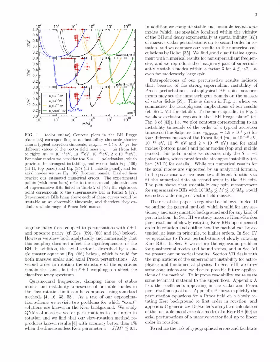
FIG. 1. (color online) Contour plots in the BH Reggeplane [43] corresponding to an instability timescale shorterthan a typical accretion timescale, τSalpeter = 4.5×10⁷ yr, fordifferent values of the vector field mass mv = µ~ (from leftto right: mv = 10−18eV, 10−19eV, 10−20eV, 2 × 10⁻²¹eV).For polar modes we consider the S = −1 polarization, whichprovides the strongest instability, and we use both Eq. (100)(fit II, top panel) and Eq. (95) (fit I, middle panel), and foraxial modes we use Eq. (95) (bottom panel). Dashed linesbracket our estimated numerical errors. The experimentalpoints (with error bars) refer to the mass and spin estimatesof supermassive BHs listed in Table 2 of [56]; the rightmostpoint corresponds to the supermassive BH in Fairall 9 [57].Supermassive BHs lying above each of these curves would beunstable on an observable timescale, and therefore they ex-clude a whole range of Proca field masses.
angular index ℓ are coupled to perturbations with ℓ ± 1and opposite parity (cf. Eqs. (59), (60) and (61) below).However we show both analytically and numerically thatthis coupling does not affect the eigenfrequencies of theBH. In addition, the axial sector is described by a sin-gle master equation [Eq. (66) below], which is valid forboth massive scalar and axial Proca perturbations. Atsecond order in rotation the structure of the equationsremain the same, but the ℓ ± 1 couplings do affect theeigenfrequency spectrum.
Quasinormal frequencies, damping times of stablemodes and instability timescales of unstable modes inthe slow-rotation limit can be computed using standardmethods [4, 16, 35, 58]. As a test of our approxima-tion scheme we revisit two problems for which “exact”solutions are known in the Kerr background. We studyQNMs of massless vector perturbations to first order inrotation and we find that our slow-rotation method re-produces known results [4] with accuracy better than 1%when the dimensionless Kerr parameter a = J/M2 . 0.3.
In addition we compute stable and unstable bound-state
modes (which are spatially localized within the vicinityof the BH and decay exponentially at spatial infinity [35])of massive scalar perturbations up to second order in ro-tation, and we compare our results to the numerical cal-culations by Dolan [35]. We find good quantitative agree-ment with numerical results for nonsuperradiant frequen-cies, and we reproduce the imaginary part of superradi-antly unstable modes within a factor 3 for a . 0.7, i.e.even for moderately large spin.
Extrapolations of our perturbative results indicatethat, because of the strong superradiant instability ofProca perturbations, astrophysical BH spin measure-ments may set the most stringent bounds on the massesof vector fields [59]. This is shown in Fig. 1, where wesummarize the astrophysical implications of our results(cf. Sect. VII for details). To be more specific, in Fig. 1we show exclusion regions in the “BH Regge plane” (cf.Fig. 3 of [43]), i.e. we plot contours corresponding to aninstability timescale of the order of a typical accretiontimescale (the Salpeter time τSalpeter = 4.5× 10⁷ yr) forfour different masses of the Proca field (mv = 10−18 eV,10−19 eV, 10−20 eV and 2 × 10⁻²¹ eV) and for axialmodes (bottom panel) and polar modes (top and middlepanels). For polar modes we consider only the S = −1polarization, which provides the strongest instability (cf.Sec. (VID) for details). While our numerical results forthe axial modes are supported by an analytical formula,in the polar case we have used two different functions tofit the numerical data at second order in the BH spin.The plot shows that essentially any spin measurementfor supermassive BHs with 106M⊙ .M . 109M⊙ wouldexclude a wide range of vector field masses.
The rest of the paper is organized as follows. In Sec. IIwe outline the general method, which is valid for any sta-tionary and axisymmetric background and for any kind ofperturbation. In Sec. III we study massive Klein-Gordonperturbations of slowly rotating Kerr BHs up to secondorder in rotation and outline how the method can be ex-tended, at least in principle, to higher orders. In Sec. IVwe specialize to Proca perturbations of slowly rotatingKerr BHs. In Sec. V we set up the eigenvalue problemfor quasinormal modes and bound states, and in Sec. VIwe present our numerical results. Section VII deals withthe implications of the superradiant instability for astro-physics and fundamental physics. In Sec. VIII we drawsome conclusions and we discuss possible future applica-tions of the method. To improve readability we relegatesome technical material to the appendices. Appendix Alists the coefficients appearing in the scalar and Procaperturbation equations. Appendix B shows explicitly theperturbation equations for a Proca field on a slowly ro-tating Kerr background to first order in rotation, andappendix C generalizes Detweiler’s analytical calculationof the unstable massive scalar modes of a Kerr BH [60] toaxial perturbations of a massive vector field up to linearorder in rotation.
To reduce the risk of typographical errors and facilitate

4
comparison with our results, we made many of our calcu-lations available online as Mathematica notebooks [61].
II. PERTURBATIONS OF A SLOWLY
ROTATING BLACK HOLE: GENERAL METHOD
In this section we outline the strategy to study generic(scalar, vector, tensor, etcetera) perturbations of any sta-tionary, axisymmetric background up to second order inthe rotation parameter, but in principle the formalismcan be extended to any order. We consider the mostgeneral stationary axisymmetric spacetime
ds20 = −H2dt2+Q2dr2+r2K2[
dϑ2 + sin2 ϑ(dϕ − Ldt)2]
,
where H , Q, K and L are functions of r and ϑ only. Tosecond order, the metric above can be expanded as [62]
ds20 =− F (r) [1 + F2] dt2 +B(r)−1
[
1 +2B2
r − 2M
]
dr2
+ r2(1 + k2)[
dϑ2 + sin2 ϑ(dϕ−dt)2]
, (1)
where M is the mass of the spacetime, is a functionof r linear in the rotation parameter, and F2, B2 and k2are functions of r and ϑ quadratic in the rotation pa-rameter. Because H , K and Q all transform like scalarsunder rotation, they can be expanded in scalar spher-ical harmonics which, due to axisymmetry, reduce tothe Legendre polynomials Pℓ(ϑ). As shown in Ref. [62],only ℓ = 0 and ℓ = 2 polynomials contribute at sec-ond order in rotation; therefore F2 can be expressed asF2(r, ϑ) = Fr(r) + Fϑ(r)P2(ϑ), and the same applies toB2(r, ϑ) and k2(r, ϑ).At first order in rotation the background (1) can be
written in the simpler form
ds20 =− F (r)dt2 +B(r)−1dr2 + r2d2Ω
− 2(r) sin2 ϑdϕdt . (2)
Note that, given a nonrotating metric, the gyromagneticfunction (r) can be computed using the approach orig-inally developed by Hartle [62]. For example, slowlyrotating Kerr BHs [cf. Eq. (18) below] correspond toF (r) = B(r) = 1 − 2M/r and = 2M2a/r, where Mand J = M2a are the mass and the angular momentumof the BH. Furthermore, the general metrics (1) and (2)encompass (among others) slowly rotating Kerr-NewmanBHs and BH solutions in modified gravity theories; thelatter have been derived analytically only up to first or-der [22, 25] (and more recently to second order [26]) inthe BH spin.Scalar, vector and tensor field equations in the back-
ground metric (1) can be linearized in the field pertur-bations (that we shall schematically denote by δX) aswell as in the BH angular momentum. We neglect termsof second order in the perturbation amplitude δX andterms of third order in the rotation parameter a, Fourier
transform the perturbations, and expand them in tensorspherical harmonics:
δXµ1...(t, r, ϑ, ϕ) = δX(i)ℓm(r)Yℓm (i)
µ1 ... e−iωt , (3)
where Yℓm (i)µ1... is a basis of scalar, vector or tensor harmon-
ics (depending on the tensorial nature of the perturbationδX) and the frequency ω is, in general, complex. The
perturbation variables δX(i)ℓm(r) can be classified as “po-
lar” or “axial” depending on their behavior under paritytransformations (ϑ → π − ϑ, ϕ → ϕ + π): polar andaxial perturbations are multiplied by (−1)ℓ and (−1)ℓ+1,respectively.With the introduction of the expansion (3), the linear
response of the system is fully characterized by the quan-
tities δX(i)ℓm(r). The perturbation equations, expanded
in spherical harmonics and Fourier transformed in time,yield a coupled system of ODEs in the perturbation func-
tions δX(i)ℓm(r). In the case of a spherically symmetric
background, perturbations with different values of (ℓ, m),as well as perturbations with opposite parity, are decou-pled. In a rotating, axially symmetric background, per-turbations with different values of m are decoupled2 butperturbations with different values of ℓ are not. However,in the limit of slow rotation there is a Laporte-like “se-lection rule” [21]: at first order in a, perturbations witha given value of ℓ are only coupled to those with ℓ±1 andopposite parity, similarly to the case of rotating stars. Atsecond order, perturbations with a given value of ℓ arealso coupled to those with ℓ± 2 and same parity, and soon.In general, the perturbation equations can be written
in the following form:
0 = Aℓ + amAℓ + a2Aℓ
+ a(QℓPℓ−1 +Qℓ+1Pℓ+1)
+ a2[
Qℓ−1QℓAℓ−2 +Qℓ+2Qℓ+1Aℓ+2
]
+O(a3) ,
(4)
0 = Pℓ + amPℓ + a2Pℓ
+ a(QℓAℓ−1 +Qℓ+1Aℓ+1)
+ a2[
Qℓ−1QℓPℓ−2 +Qℓ+2Qℓ+1Pℓ+2
]
+O(a3) .
(5)
Here
Qℓ =
√
ℓ2 −m2
4ℓ2 − 1; (6)
Aℓ, Aℓ, Aℓ, Aℓ, Aℓ are linear combinations of the axialperturbations and of their derivatives, with multipolar
2 From now on we will append the relevant multipolar index ℓ toany perturbation variable but we will omit the index m, becausein an axisymmetric background it is possible to decouple theperturbation equations so that all quantities have the same valueof m.

5
index ℓ; similarly, Pℓ, Pℓ, Pℓ, Pℓ, Pℓ are linear combina-tions of the polar perturbations and of their derivatives,with index ℓ. The dimensionless parameter a keeps trackof the order of the various terms in the slow-rotation ex-pansion.The structure of Eqs. (4)–(5) is the following. Pertur-
bations with a given parity and index ℓ are coupled to:(i) perturbations with opposite parity and index ℓ± 1 atorder a; (ii) perturbations with same parity and same in-dex ℓ up to order a2; (iii) perturbations with same parityand index ℓ± 2 at order a2.From Eq. (6) it follows that Q±m = 0, and therefore
if |m| = ℓ the coupling of perturbations with index ℓ toperturbations with indices ℓ− 1 and ℓ− 2 is suppressed.Since the contribution |m| = ℓ dominates the linear re-sponse of the system, this general property of Eqs. (4)–(5) is reminiscent of a “propensity rule” in atomic theory,which states that transitions ℓ → ℓ + 1 are strongly fa-vored over transitions ℓ → ℓ − 1 (cf. [21] and referencestherein).Due to the coupling between different multipolar in-
dices, the spectrum of the solutions of Eqs. (4)–(5) isextremely rich. However, if we are interested in the char-acteristic modes of the slowly rotating background to firstor to second order in a, the perturbation equations canbe considerably simplified. We discuss the truncation tofirst and to second order in the next two sections, respec-tively.
A. Eigenvalue spectrum to first order
Let us consider the first order expansion of Eqs. (4) and(5). We expand all quantities to first order and we ignore
the terms Aℓ, Aℓ, Pℓ and Pℓ, which are multiplied by a2.Furthermore the terms (Pℓ, Aℓ) in Eqs. (4) and (5) donot contribute to the eigenfrequencies at first order ina. This was first shown by Kojima [19] using symmetryarguments for the axisymmetric case m = 0. Here weextend his argument to any value of m, for the genericset of equations (4) and (5). Let us start by noting that,at first order, Eqs. (4) and (5) are invariant under thesimultaneous transformations
aℓm → ∓aℓ−m , pℓm → ±pℓ−m , (7a)
a→ −a , m→ −m, (7b)
where aℓm (pℓm) schematically denotes all of the axial(polar) perturbation variables with indices (ℓ,m). Theinvariance follows from the linearity of the terms inEqs. (4) and (5) and from the fact that the Qℓ’s are evenfunctions of m. The boundary conditions that define thecharacteristic modes of the BH are also invariant underthe transformation above (cf. Eqs. (72) and (77) below).Therefore in the slow-rotation limit the eigenfrequenciescan be expanded as
ω = ω0 +mω1a+ ω2a2 +O(a3) , (8)
where ω0 is the eigenfrequency of the nonrotating space-time and ωn is the n-th order correction (note that ω1
and ω2 are generically polynomials in m but, due to theabove symmetry, ω1 is an even polynomial). Crucially,only the terms (Pℓ, Aℓ) in Eqs. (4) and (5) can contributeto ω1. Indeed, due to the factor a in front of all terms(Pℓ, Aℓ, Pℓ, Aℓ) and to their linearity, at first order in awe can simply take the zeroth order (in rotation) expan-sion of these terms. That is, to our level of approxima-tion the terms (Pℓ, Aℓ, Pℓ, Aℓ) in Eqs. (4) and (5) onlycontain the perturbations of the nonrotating, sphericallysymmetric background. Since the latter do not explicitlydepend on m, the m dependence in Eq. (8) can only arisefrom the terms (Pℓ, Aℓ) to zeroth order (recall that theQℓ’s are even functions of m, so they do not contribute).In the case of slowly rotating stars, this argument is re-
inforced by numerical simulations for the m = 0 axisym-metric modes [19] and in the general nonaxisymmetriccase [63], which show that the coupling terms do not af-fect the first order corrections to the QNMs. In this workwe shall verify that the same result holds also for mass-less vector (e.g. electromagnetic) modes and for Procamodes of a Kerr BH. If we are interested in the modes ofthe rotating background to O(a) the coupling terms cantherefore be neglected, and the eigenvalue problem canbe written in the form
Aℓ + amAℓ = 0 , (9)
Pℓ + amPℓ = 0 . (10)
In these equations the polar and axial perturbations (aswell as perturbations with different values of the har-monic indices) are decoupled from each other, and canbe studied independently.
B. Eigenvalue spectrum to second order
For what concerns the calculation of the eigenfrequen-cies to second order in a, the equations above can besimplified as follows. To begin with, we remark that allof the coefficients in Eqs. (4) and (5) are linear com-binations of axial or polar perturbation functions, aℓm,pℓm, respectively. These functions can be expanded inthe rotation parameter as
aℓm = a(0)ℓm + a a
(1)ℓm + a2a
(2)ℓm
pℓm = p(0)ℓm + a p
(1)ℓm + a2p
(2)ℓm . (11)
The terms Aℓ±2 and Pℓ±2 are multiplied by factors a2,so they only depend on the zeroth-order perturbation
functions, a(0)ℓm, p
(0)ℓm. The terms Aℓ±1 and Pℓ±1 are mul-
tiplied by factors a, so they only depend on zeroth- and
first-order perturbation functions a(0)ℓm, p
(0)ℓm, a
(1)ℓm, p
(1)ℓm.
Since in the nonrotating limit axial and polar perturba-tions are decoupled, a possible consistent set of solutions
of the system (4)–(5) has a(0)ℓ±2m ≡ 0; another consis-
tent set of solutions of the same system has p(0)ℓ±2m ≡ 0.

6
Such solutions, which we can call, following Refs. [29, 30],“axial-led” and “polar-led” perturbations respectively,can be found by solving the following subsets of the equa-tions (4)–(5):
Aℓ + amAℓ + a2Aℓ + a(QℓPℓ−1 +Qℓ+1Pℓ+1) = 0 ,
(12)
Pℓ+1 + amPℓ+1 + aQℓ+1Aℓ = 0 , (13)
Pℓ−1 + amPℓ−1 + aQℓAℓ = 0 , (14)
and
Pℓ + amPℓ + a2Pℓ + a(QℓAℓ−1 +Qℓ+1Aℓ+1) = 0 ,
(15)
Aℓ+1 + amAℓ+1 + aQℓ+1Pℓ = 0 , (16)
Aℓ−1 + amAℓ−1 + aQℓPℓ = 0 . (17)
In the second and third equations of the two systemsabove we have dropped the Aℓ±2 and Pℓ±2 terms, be-cause these only enter at zeroth order, and we have set
a(0)ℓ±2m ≡ 0 and p
(0)ℓ±2m ≡ 0.
Interestingly, within this perturbative scheme a notionof “conserved quantum number” ℓ is still meaningful,even though, for any given ℓ, rotation couples terms withopposite parity and different multipolar index. In themost relevant case from the point of view of superradiantinstabilities, i.e. the case ℓ = m, the last equations (14)and (17) are automatically satisfied, becauseQm = 0 andperturbations with ℓ < m automatically vanish.It is worth stressing that, even though in principle
there may be modes which do not belong to the classes of“axial-led” or “polar-led” perturbations, all solutions be-longing to one of these classes which fulfill the appropri-ate boundary conditions defining QNMs or bound statesare also solutions of the full system (4)–(5) and belongto the eigenspectrum (up to second order in the rota-tion rate). This is particularly relevant since, as we shallshow, these classes contain also superradiantly unstablemodes.In the case of massive scalar perturbations, as we show
in the next section, the coupling to ℓ±2 can be eliminatedby defining a suitable linear combination of the eigen-functions with different multipolar indices [cf. Eq. (37)],so that our procedure allows us to compute the entireBH spectrum up to second order. By a similar, suitable“rotation” in eigenfunction space it may be possible torecast Eqs. (4)–(5) in the forms (12)–(14) and (15)–(17),but we did not find a general proof of this conjecture. Ifthe conjecture is correct, studying the “axial-led” and“polar-led” systems may be sufficient to describe the en-
tire BH spectrum at second order in rotation.To summarize, the eigenfrequencies (or at least a sub-
set of the eigenfrequencies) of the general system (4)–(5)can be found, at first order in a, by solving the two de-coupled sets (9) and (10) for axial and polar perturba-tions, respectively. At second order in a we must solveeither the set (12)–(14) or the set (15)–(17) for “axial-led” and “polar-led” modes, respectively. We conclude
this section by noting that this procedure can be appliedto any slowly rotating spacetime and to any kind of per-turbation. For concreteness, in the next section we shallspecialize the method to the case of massive scalar andvector perturbations of the Kerr metric.
III. MASSIVE SCALAR PERTURBATIONS OF
SLOWLY ROTATING KERR BLACK HOLES
In order to illustrate how the slow-rotation expansionworks, in this section we begin by working out the sim-plest case. We consider the massive Klein-Gordon equa-tion for a scalar field perturbation φ around a rotatingBH, and we work out the perturbation equations up tosecond order in rotation. The formalism applies to ageneric stationary and axisymmetric background, but itis natural to focus on the case of interest in general rel-ativity, i.e. the Kerr metric in Boyer-Lindquist coordi-nates:
ds2Kerr = −(
1− 2Mr
Σ
)
dt2 +Σ
∆dr2 − 4rM2
Σa sin2 ϑdϕdt
+Σdϑ2 +
[
(r2 +M2a2) sin2 ϑ+2rM3
Σa2 sin4 ϑ
]
dϕ2 ,
(18)
where Σ = r2 +M2a2 cos2 ϑ, ∆ = (r − r+)(r − r−) and
r± = M(1 ±√1− a2). In what follows we shall ex-
pand the metric and all other quantities of interest tosecond order in a. At this order, the event horizon r+,the Cauchy horizon r− and the outer ergosphere rS+ canbe written in the form
r+ = 2M
(
1− a2
4
)
, r− =Ma2
2,
rS+ = 2M
(
1− cos2 ϑa2
4
)
. (19)
In particular, note that second-order corrections are nec-essary for the ergoregion to be located outside the eventhorizon.The massive Klein-Gordon equation reads
φ = µ2φ , (20)
where ms = µ~ is the mass of the scalar field. We de-compose the field in spherical harmonics:
φ =∑
ℓm
Ψℓ(r)√r2 + a2M2
e−iωtY ℓ(ϑ, ϕ) , (21)
and expand the square root above to second order in a.Schematically, we obtain the following equation:
AℓYℓ +Dℓ cos
2 ϑY ℓ = 0 , (22)
where a sum over (ℓ,m) is implicit, and the explicit formof Aℓ and Dℓ is given in Appendix A1. The crucial point

7
is that Dℓ is proportional to a2, so the second term inthe equation above is zero to first order in rotation. Ifwe consider a first-order expansion in rotation the scalarequation is already decoupled, and it can be cast in theform
D2Ψℓ −[
4mM2aω
r3+ F
2M
r3
]
Ψℓ = 0 , (23)
where F = 1 − 2M/r, dr/dr∗ = F and we defined theoperator [16]
D2 =d2
dr2∗+ ω2 − F
[
ℓ(ℓ+ 1)
r2+ µ2
]
. (24)
Equation (23) coincides with Teukolsky’s master equa-tion [13] for spin s = 0 perturbations expanded to first or-der in a. The coupling to perturbations with indices ℓ±1vanishes for a simple reason: Klein-Gordon perturbationsare polar quantities, and at first order the Laporte-likeselection rule implies that polar perturbations with in-dex ℓ should couple to axial perturbations with ℓ ± 1,but the latter are absent in the spin-0 case. At secondorder, perturbations with harmonic index ℓ are coupledto perturbations with the same parity and ℓ±2, but thiscoupling does not contribute to the eigenfrequencies forthe reasons discussed in the previous section. Thereforewe must solve a single scalar equation for given values ofℓ and m, that we write schematically as
Pℓ + amPℓ + a2Pℓ = 0 . (25)
In order to confirm this general result, let us separatethe angular part of Eq. (22). This can be achieved byusing the identities [17]
cosϑY ℓ = Qℓ+1Yℓ+1 +QℓY
ℓ−1 , (26)
sinϑ∂ϑYℓ = Qℓ+1ℓY
ℓ+1 −Qℓ(ℓ+ 1)Y ℓ−1 , (27)
cos2 ϑY ℓ =(
Q2ℓ+1 +Q2
ℓ
)
Y ℓ
+Qℓ+1Qℓ+2Yℓ+2 +QℓQℓ−1Y
ℓ−2 ,
(28)
cosϑ sinϑ∂ϑYℓ =
(
ℓQ2ℓ+1 − (ℓ+ 1)Q2
ℓ
)
Y ℓ
+Qℓ+1Qℓ+2ℓYℓ+2
−QℓQℓ−1(ℓ+ 1)Y ℓ−2 , (29)
as well as the orthogonality property of scalar sphericalharmonics:
∫
Y ℓY ∗ ℓ′dΩ = δℓℓ′
. (30)
The result reads, schematically,
Aℓ + (Q2ℓ+1 +Q2
ℓ)Dℓ
+Qℓ−1QℓDℓ−2 +Qℓ+2Qℓ+1Dℓ+2 = 0 . (31)
By repeated use of the identity (26) we can separatethe perturbation equations at any order in a. Indeed,because of the expansion in a, only combinations of the
form (cosϑ)nY ℓ will appear. As we discuss in the nextsection this is also true for spin-1 or spin-2 perturbations,except that now the perturbation equations will containcombinations of vector and tensor spherical harmonics,and this introduces terms such as (sinϑ)n∂ϑY
ℓ, whichcan be decoupled in a similar fashion by repeated appli-cation of the identities listed above. This procedure iswell known in quantum mechanics, and the coefficientsQℓ are related to the usual Clebsch-Gordan coefficients.Using the explicit form of the coefficients given in Ap-
pendix A1, the field equations (31) schematically read
d2Ψℓ
dr2∗+ VℓΨℓ + a2
[
Uℓ+2Ψℓ+2 + Uℓ−2Ψℓ−2
+Wℓ+2d2Ψℓ+2
dr2∗+Wℓ−2
d2Ψℓ−2
dr2∗
]
= 0 ,
(32)
where we have defined the tortoise coordinate viadr/dr∗ ≡ f = ∆/(r2 + a2) (expanded at second order)and V , U andW are some potentials, whose explicit formis not needed here.Note that the coupling to the ℓ±2 terms is proportional
to a2. For a calculation accurate to second order in a theterms in parenthesis can be evaluated at zeroth order,
and therefore the functions Ψ(0)ℓ±2 must be solutions of
d2Ψ(0)ℓ±2
dr2∗+ V
(0)ℓ±2Ψ
(0)ℓ±2 = 0 . (33)
By substituting these relations in Eq. (32) we get
d2Ψℓ
dr2∗+ VℓΨℓ+a
2(
U(0)ℓ+2 − V
(0)ℓ+2W
(0)ℓ+2
)
Ψ(0)ℓ+2
+a2(
U(0)ℓ−2 − V
(0)ℓ−2W
(0)ℓ−2
)
Ψ(0)ℓ−2 = 0 .(34)
Finally, making use of the expressions for V , U and W ,the field equations can be reduced to
d2Ψℓ
dr2∗+ VℓΨℓ =
a2M2(r − 2M)(
µ2 − ω2)
r3
×[
Qℓ+1Qℓ+2Ψ(0)ℓ+2 +Qℓ−1QℓΨ
(0)ℓ−2
]
, (35)
where the potential is given by
Vℓ= ω2 −(
1− 2M
r
)[
ℓ(ℓ+ 1)
r2+
2M
r3+ µ2
]
−4amωM2
r3
+a2M2
r6[
−24M2 − 4Mr(
ℓ(ℓ+ 1)− 3 + r2µ2)
+2Mr3ω2 + r2(
ℓ(ℓ+ 1) +m2 + r2(µ2 − ω2)− 1)
−r3(r − 2M)(µ2 − ω2)(
Q2ℓ +Q2
ℓ+1
)]
. (36)
As we previously discussed, the couplings to terms withindices ℓ ± 2 can be neglected in the calculation of the

8
modes. In the scalar case this can be shown explicitly asfollows. If we define
Zℓ = ψℓ − a2 [cℓ+2ψℓ+2 − cℓψℓ−2] , (37)
where
cℓ =M2
(
µ2 − ω2)
Qℓ−1Qℓ
2(2ℓ− 1), (38)
then, at second order in rotation, Eq. (35) can be writtenas a single equation for Zℓ:
d2Zℓ
dr2∗+ VℓZℓ = 0 , (39)
which can be solved by standard methods. This equationcoincides with Teukolsky’s master equation [13] for spins = 0 perturbations expanded at second order in a. Thisis a nontrivial consistency check for the slow-rotation ex-pansion. In particular, the coefficients Qℓ in Eq. (36)agree with an expansion of Teukolsky’s spheroidal eigen-values to second order in a [64]. In fact, by extendingour procedure to arbitrary order in a we can reconstructthe Teukolsky scalar potential order by order. This canbe viewed as an independent check of the standard pro-cedure, which consists of expanding the angular equationto obtain the angular eigenfrequencies (see [64] and ref-erences therein).In addition, as discussed in the previous section, the
fact that neglecting the ℓ± 2 couplings is equivalent to afield redefinition implies that the entire BH spectrum of(massive scalar) QNMs and bound states can be foundby neglecting those couplings.Finally, the near-horizon behavior of Eq. (39) reads
Zℓ ∼ e−i kHr∗ , (40)
where kH = ω−mΩH and ΩH ∼ a/(4M)+O(a3). Notethat, by virtue of the second order expansion, we getprecisely Vℓ ∼ k2H close to the horizon.The possibility to obtain a single equation for any given
ℓ and m is a special feature of scalar perturbations. Theunderlying reason is that scalar perturbations have defi-nite parity, so the mixing between perturbations of differ-ent parity cannot occur. As we show in the next section,this property does not necessarily hold for perturbationsof higher spin.
IV. MASSIVE VECTOR PERTURBATIONS OF
SLOWLY ROTATING KERR BLACK HOLES
The field equations of a massive vector field (alsoknown as Proca’s equation) read
Πν ≡ ∇σFσν − µ2Aν = 0 , (41)
where Fµν = ∂µAν−∂νAµ and Aµ is the vector potential.Maxwell’s equations are recovered when µ = mv/~ = 0,
where mv is the mass of the vector field. Note that, as aconsequence of Eq. (41), the Lorenz condition ∇µA
µ = 0is automatically satisfied, i.e. in the massive case there isno gauge freedom and the field Aµ propagates 2s+1 = 3degrees of freedom [16].In the µ = 0 case, Teukolsky showed that the equa-
tions for spin-1 perturbations around a Kerr BH are sep-arable [13], the angular part being described by spin-1spheroidal harmonics. In the case of a massive field theseparation does not appear to be possible, and one is leftwith a set of coupled partial differential equations. Toavoid these difficulties we shall consider the slow-rotationlimit of the Kerr metric and apply the approach describedin Sec. II. The procedure is equivalent in spirit to thatdescribed for scalar perturbations, but it is more involveddue to the spin-1 nature of the vector field.
A. Harmonic expansion of the Proca equation on a
slowly rotating background
Following the notation of [63, 65] we set xµ = (t, r, xb)with xb = (ϑ, ϕ). We also introduce the metric of thetwo-sphere γab = diag(1, sin2 ϑ).Any vector field can be decomposed in a set of vector
spherical harmonics [65]
Yℓb =
(
∂ϑYℓ, ∂ϕY
ℓ)
,
Sℓb =
(
1
sinϑ∂ϕY
ℓ,− sinϑ∂ϑYℓ
)
, (42)
where Y ℓ(ϑ, ϕ) are the scalar spherical harmonics. Weexpand the electromagnetic potential as follows [16]:
δAµ(t, r, ϑ, ϕ) =∑
ℓ,m
00
uℓ(4)Sℓb/Λ
+∑
ℓ,m
uℓ(1)Yℓ/r
uℓ(2)Yℓ/(rf)
uℓ(3)Yℓb/Λ
,
(43)where Λ = ℓ(ℓ + 1). Because of their transformationproperties under parity, the functions uℓ(i) belong to the
polar sector when i = 1, 2, 3, and to the axial sectorwhen i = 4. In the nonrotating case the two sectors aredecoupled [16]. The Proca equation (41), linearized inthe perturbations uℓ(i) (i = 1, 2, 3, 4), can be written in
the following form:
δΠI ≡(
A(I)ℓ + A
(I)ℓ cosϑ+D
(I)ℓ cos2 ϑ
)
Y ℓ
+(
B(I)ℓ + B
(I)ℓ cosϑ
)
sinϑ∂ϑYℓ = 0 , (44)
δΠϑ ≡(
αℓ + ρℓ sin2 ϑ
)
∂ϑYℓ − imβℓ
Y ℓ
sinϑ
+(ηℓ + σℓ cosϑ) sinϑYℓ = 0 , (45)
δΠϕ
sinϑ≡
(
βℓ + γℓ sin2 ϑ
)
∂ϑYℓ + imαℓ
Y ℓ
sinϑ
+(ζℓ + λℓ cosϑ) sinϑYℓ = 0 , (46)
where a sum over (ℓ,m) is implicit and I denotes eitherthe t component or the r component. The various radial

9
coefficients in the equations above are given in terms ofthe perturbation functions uℓ(i) in Appendix A2.
The perturbation equations (44)–(46) can be simpli-fied by using the Lorenz identity ∇µA
µ = 0. To secondorder in rotation, and for the background metric (18),this condition reads
δΠL ≡(
A(2)ℓ + A
(2)ℓ cosϑ+D
(2)ℓ cos2 ϑ
)
Y ℓ
+(
B(2)ℓ + B
(2)ℓ cosϑ
)
sinϑ∂ϑYℓ = 0 , (47)
where the various coefficients are again listed in Ap-pendix A2.
Each of the coefficients in Eqs. (44)–(47) is a linearcombination of perturbation functions with either polaror axial parity (cf. Appendix A2). Therefore we candivide them into two sets:
Polar: A(j)ℓ , αℓ , ζℓ , Bℓ , Dℓ , ρℓ , σℓ ,
Axial: A(j)ℓ , B
(j)ℓ , βℓ , ηℓ , λℓ , γℓ ,
where j = 0, 1, 2. In order to separate the angular vari-ables in Eqs. (44)–(47) we compute the following inte-grals:
∫
δΠIY∗ ℓdΩ , (I = t, r, L) ; (48a)
∫
δΠaY∗ ℓb γabdΩ , (a , b = ϑ, ϕ) ; (48b)
∫
δΠaS∗ ℓb γabdΩ , (a , b = ϑ, ϕ) . (48c)
Using the orthogonality properties of scalar and vectorharmonics, Eq. (30), the relations
∫
YℓbY
∗ ℓ′
b γabdΩ =
∫
SℓbS
∗ ℓ′
b γabdΩ = Λδℓℓ′
,
∫
YℓbS
∗ ℓ′
b γabdΩ = 0 , (49)
as well as the identities (26)–(29), we find the following
radial equations:
A(I)ℓ +Q2
ℓ+1
[
D(I)ℓ + ℓB
(I)ℓ
]
+Q2ℓ
[
D(I)ℓ − (ℓ+ 1)B
(I)ℓ
]
+
Qℓ
[
A(I)ℓ−1 + (ℓ − 1)B
(I)ℓ−1
]
+Qℓ+1
[
A(I)ℓ+1 − (ℓ+ 2)B
(I)ℓ+1
]
+
Qℓ−1Qℓ
[
D(I)ℓ−2 + (ℓ − 2)B
(I)ℓ−2
]
+Qℓ+2Qℓ+1
[
D(I)ℓ+2 − (ℓ + 3)B
(I)ℓ+2
]
= 0 , (50)
Λαℓ − imζℓ +Q2ℓ+1ℓ [ℓρℓ + σℓ] +Q2
ℓ(ℓ+ 1) [(ℓ+ 1)ρℓ − σℓ]
+Qℓ [−(ℓ+ 1)ηℓ−1 − im((ℓ − 1)γℓ−1 + λℓ−1)]
+Qℓ+1 [ℓηℓ+1 + im((ℓ + 2)γℓ+1 − λℓ+1)]
−Qℓ−1Qℓ(ℓ+ 1) [(ℓ− 2)ρℓ−2 + σℓ−2]
+Qℓ+2Qℓ+1ℓ [−(ℓ+ 3)ρℓ+2 + σℓ+2] = 0 , (51)
Λβℓ + imηℓ +Q2ℓ+1ℓ [ℓγℓ + λℓ] +Q2
ℓ(ℓ + 1) [(ℓ+ 1)γℓ − λℓ]
+Qℓ [−(ℓ+ 1)ζℓ−1 + im((ℓ − 1)ρℓ−1 + σℓ−1)]
+Qℓ+1 [ℓζℓ+1 − im((ℓ + 2)ρℓ+1 − σℓ+1)]
−Qℓ−1Qℓ(ℓ+ 1) [(ℓ− 2)γℓ−2 + λℓ−2]
+Qℓ+2Qℓ+1ℓ [−(ℓ+ 3)γℓ+2 + λℓ+2] = 0 . (52)
Note that Eqs. (50)–(52) have exactly the same structureas Eqs. (4)–(5).
B. Proca perturbation equations at first order
In order to make the equations more tractable, in thissection we focus on the first-order corrections only. Thesecond-order analysis is presented in Sec. IVC below. Atfirst order, Eqs. (50)–(52) simplify to
A(I)ℓ +Qℓ
[
A(I)ℓ−1 + (ℓ − 1)B
(I)ℓ−1
]
+Qℓ+1
[
A(I)ℓ+1 − (ℓ+ 2)B
(I)ℓ+1
]
= 0 , (53)
Λαℓ − imζℓ
−Qℓ(ℓ + 1)ηℓ−1 +Qℓ+1ℓηℓ+1 = 0 , (54)
Λβℓ + imηℓ
−Qℓ(ℓ + 1)ζℓ−1 +Qℓ+1ℓζℓ+1 = 0 , (55)
where now the coefficients are linear in a.To begin with, let us focus on the equations for
monopole perturbations, ℓ = m = 0. The longitudi-nal mode of a massive vector field (unlike the masslesscase) is dynamical. Since m = 0, the monopole only ex-cites axisymmetric modes. In the nonrotating case theseare described by a single equation belonging to the polarsector [55] (see also [16]); for ℓ = 0, only the first twocomponents u0(1) and u0(2) are defined. However, in the
slowly rotating case these components are coupled to theℓ = 1 axial component u1(4) through Eq. (53).
When ℓ = m = 0, Q0 = 0 and Eq. (53) reduces to
A(I)0 +Q1
[
A(I)1 − 2B
(I)1
]
= 0 , (56)
10
where I = 0, 1, 2. This is an extreme example of the“propensity rule” discussed in the general case: at firstorder the monopole is only coupled with axial perturba-tions with ℓ = 1. Using the explicit form of the coeffi-cients A(I), A(I), B(I) given in Appendix A2 (truncatedat first order), the equations above can be written as asingle equation for u0(2):
[
d2
dr2∗+ ω2 − F
(
2(r − 3M)
r3+ µ2
)]
u0(2)
=2i√3aM2ωF
r3u1(4) , (57)
where at first order the tortoise coordinate r∗ is the sameas in the Schwarzschild case, and it is defined by dr/dr∗ =F . The source term u1(4) is the solution of Eq. (53) with
ℓ = 1. To first order in a we can approximate u1(4) (that
is multiplied by a in the source term) by its zeroth-orderexpansion in a, which is a solution of
d2
dr2∗+ ω2 − F
[
2
r2+ µ2
]
u1(4) = 0 . (58)
Note that Eq. (58) is precisely the axial perturbationequation in the nonrotating case for ℓ = 1 [16]. Eqs. (57)and (58) fully describe the dynamics of the polar ℓ = 0perturbations in the slow-rotation approximation. As weproved in Sec. II, the coupling on the right-hand side ofEq. (57) does not affect the QNMs to first order in rota-tion. In addition, since for the monopole m = 0, to thisorder the frequency is the same as in the Schwarzschildcase, which is extensively discussed in Ref. [16].Let us now turn to modes with ℓ > 0. The equations
for ℓ > 0 at first order in a are derived in Appendix Bby using the Lorenz condition (B2) in order to eliminateuℓ(1). The polar sector is fully described by the system
D2uℓ(2) −
2F
r2
(
1− 3M
r
)
[
uℓ(2) − uℓ(3)
]
=2aM2m
Λr5ω
[
Λ(
2r2ω2 + 3F 2)
uℓ(2)
+3F(
rΛFu′ℓ(2) −
(
r2ω2 + ΛF)
uℓ(3)
)]
− 6i aM2Fω
Λr3
[
(ℓ + 1)Qℓuℓ−1(4) − ℓQℓ+1u
ℓ+1(4)
]
, (59)
D2uℓ(3) +
2FΛ
r2uℓ(2) =
2aM2m
r5ω
[
2r2ω2uℓ(3) + 3rF 2u′ℓ(3) − 3
(
Λ + r2µ2)
Fuℓ(2)
]
,
(60)
where here and in the following a prime denotes deriva-tion with respect to r and the operator D2 is definedin Eq. (24). Note that while Eq. (60) only involves po-lar perturbations, in Eq. (59) we also have a coupling to
uℓ±1(4) .
On the other hand, the axial sector leads to
D2uℓ(4) −
4aM2mω
r3uℓ(4)
= −6i aM2F
r5ω
[
(ℓ+ 1)Qℓmψℓ−1 − ℓQℓ+1mψ
ℓ+1]
(61)
(see Appendix B for details), where we have defined thepolar function
ψℓ =(
Λ + r2µ2)
uℓ(2) − (r − 2M)u′ℓ(3) . (62)
Note that this term is similar to Eq.(25) in Ref. [16]. Asexpected, the axial perturbation uℓ(4) is coupled to the
polar functions with ℓ± 1. Equations (59), (60) and (61)describe the massive vector perturbations of a Kerr BHto first order in a for ℓ > 0. These equations reduce tothose in Ref. [16] when a = 0.Since the right-hand side of Eq. (61) is proportional to
a, in our perturbative framework we can first solve foruℓ±1(2) and uℓ±1
(3) to zeroth order in the rotation rate, and
then use these solutions as a source term in Eq. (61). Aswe proved in Sec. II, the coupling on the right-hand sideof Eq. (61) does not affect the QNMs to first order in rota-tion. In Sec. VI we shall verify this property numerically.Therefore, for the purpose of computing eigenfrequenciesto first order in a we can simply consider the followingpolar equations:
D2uℓ(2) −
2F
r2
(
1− 3M
r
)
[
uℓ(2) − uℓ(3)
]
=2aM2m
Λr5ω
[
Λ(
2r2ω2 + 3F 2)
uℓ(2)
+3F(
rΛFu′ℓ(2) −
(
r2ω2 + ΛF)
uℓ(3)
)]
, (63)
D2uℓ(3) +
2FΛ
r2uℓ(2) =
2aM2m
r5ω
[
2r2ω2uℓ(3) + 3rF 2u′ℓ(3) − 3
(
Λ + r2µ2)
Fuℓ(2)
]
,
(64)
as well as the decoupled axial equation
D2uℓ(4) −
4aM2mω
r3uℓ(4) = 0 . (65)
Within our perturbative scheme, any eigenfrequency ofEq. (65) is also a solution of the coupled Eq. (61) as
long as uℓ±1(2) = uℓ±1
(3) = 0, which is a trivial solution of
Eqs. (59) and (60) for ℓ ± 1 at zeroth order. Further-more, consistently with our argument in Sec. II, we havechecked that there are no other modes to order O(a) (cf.Sec. VI).Note the similarity between Eq. (65), describing axial
Proca modes, and Eq. (23) for massive scalar pertur-bations. Indeed, one can show that the generalizationof Eq. (65) to the background metric (2) (i.e. withoutspecializing to the slowly rotating Kerr metric) can be

11
written in a form that includes also massive scalar per-turbations. This “master equation” reads
FBΨ′′ℓ +
1
2[B′F + F ′B] Ψ′
ℓ +
[
ω2 − 2m(r)ω
r2
−F(
Λ
r2+ µ2 + (1− s2)
B′
2r+BF ′
2rF
)]
Ψℓ = 0 ,
(66)
and it can be simplified by introducing a generalized tor-toise coordinate y(r) such that dr/dy =
√FB. In the
equation above s is the spin of the perturbation (s = 0for scalar perturbations and s = ±1 for vector perturba-tions with axial parity). In the nonrotating case Eq. (66)is exact; it also includes gravitational perturbations of aSchwarzschild BH if s = ±2 and F = B = 1− 2M/r. Inthe slowly rotating case Eq. (66) is a complete descrip-tion of massive scalar perturbations for s = 0, whereas fors = ±1 it describes the axial sector without the ℓ→ ℓ±1couplings, i.e. it is a generalization of Eq. (65).
C. Proca perturbation equations at second order
In this section we briefly present the derivation of theProca eigenvalue problem to second order in a.
By using the Lorenz condition to eliminate the spuri-ous uℓ(1) mode, Eqs. (50)–(52) can be written as
DAΨAℓ +VAΨA
ℓ = 0 , (67)
DPΨPℓ +VPΨP
ℓ = 0 , (68)
whereDA,P are second order differential operators,VA,P
are matrices, ΨAℓ = (uℓ(4), u
ℓ±1(2) , u
ℓ±1(3) , u
ℓ±2(4) ) and ΨP
ℓ =
(uℓ(2), uℓ(3), u
ℓ±1(4) , u
ℓ±2(2) , u
ℓ±2(3) ). The explicit form of the
equations above is quite lengthy; therefore we do notshow it in this article, but we make it available online [61].It can be obtained using the procedure explained aboveand the coefficients listed in Appendix A2. The func-tion uℓ(1) can be obtained from the Lorenz condition once
the three dynamical degrees of freedom are known. Notethat Eqs. (70)-(71) are particular cases of Eqs. (12)-(14)and Eqs. (15)-(17), respectively.
If we are interested in the eigenfrequencies up to sec-ond order in a we can drop the couplings to ℓ ± 2 per-turbations, for reasons discussed in Sec. II. Therefore, a
consistent subset of Eqs. (50)–(52) reads
0 = A(i)ℓ +Q2
ℓ+1
[
D(i)ℓ + ℓB
(i)ℓ
]
+Q2ℓ
[
D(i)ℓ − (ℓ+ 1)B
(i)ℓ
]
+Qℓ
[
A(i)ℓ−1 + (ℓ− 1)B
(i)ℓ−1
]
+Qℓ+1
[
A(i)ℓ+1 − (ℓ+ 2)B
(i)ℓ+1
]
,
0 = Λαℓ − imζℓ +Q2ℓ+1ℓ [ℓρℓ + σℓ]
+Q2ℓ(ℓ+ 1) [(ℓ+ 1)ρℓ + σℓ]
+Qℓ [−(ℓ+ 1)ηℓ−1 − im((ℓ − 1)γℓ−1 + λℓ−1)]
+Qℓ+1 [ℓηℓ+1 + im((ℓ + 2)γℓ+1 − λℓ+1)] ,
0 = Λβℓ + imηℓ +Q2ℓ+1ℓ [ℓγℓ + λℓ]
+Q2ℓ(ℓ+ 1) [(ℓ+ 1)γℓ + λℓ]
+Qℓ [−(ℓ+ 1)ζℓ−1 + im((ℓ− 1)ρℓ−1 + σℓ−1)]
+Qℓ+1 [ℓζℓ+1 − im((ℓ+ 2)ρℓ+1 − σℓ+1)] . (69)
As in the scalar case, the second-order coefficients gener-ally contain second derivatives of the perturbation func-
tions, i.e. u′′ℓ(i), u
′′ℓ±1(i) and u′′
ℓ±2(i) . Since the coefficients
are already of second order, we can use the perturbationequations in the nonrotating limit in order to eliminatethese second derivatives. After some manipulation we getthe final two sets of equations, that can be schematicallywritten as
D′AΥA
ℓ +V′AΥA
ℓ = 0 , (70)
D′PΥP
ℓ +V′PΥP
ℓ = 0 , (71)
where D′A,P are second order differential operators,
ΥAℓ = (uℓ(4), u
ℓ±1(2) , u
ℓ±1(3) ), ΥP
ℓ = (uℓ(2), uℓ(3), u
ℓ±1(4) ), and
V′A,P are matrices.We remark that for a given value of ℓ and m, ΥA and
ΥP are five- and four-dimensional vectors, respectively,while ΨA and ΨP in Eqs. (67) and (68) are seven- andeight-dimensional vectors, respectively. This is a veryconvenient simplification, because large systems of equa-tions are computationally more demanding. Furthermorethe couplings to perturbations with index ℓ− 1 vanish ifℓ = m, because as usual the factors Qm = 0, and in thiscase we are left with two subsystems of dimension three.
V. THE EIGENVALUE PROBLEM FOR
QUASINORMAL MODES AND BOUND STATES
One of the key advantages of the slow-rotation approx-imation is that the perturbation equations can be solvedusing well-known numerical approaches. The integrationproceeds exactly in the same way as in the nonrotatingcase. For example, for Proca perturbations of a slowly ro-tating Kerr BH we can compute the characteristic modesby following a procedure similar to the Schwarzschild casediscussed in Ref. [16], as follows.The perturbation equations (70)–(71), together with
appropriate boundary conditions at the horizon and atinfinity, form an eigenvalue problem for the frequency
12
spectrum. In the near-horizon limit, DA,P → d2/dr2∗and VA,P → (ω − mΩH)2, so that at the horizon weimpose purely ingoing-wave boundary conditions:
uℓ(i) ∼ uℓ(i)He−i kHr∗ , (72)
where uℓ(i)H is a constant and
kH = ω −mΩH = ω − ma
4M+O(a3) . (73)
We have introduced the horizon angular frequency ΩH =a/(2Mr+) and expanded it to second order.In the massless case, due to the boundary condi-
tion (72), superradiant scattering for scalar, electromag-netic and gravitational perturbations is possible whenωR < mΩH [66], i.e. (to second order in rotation) when
a >4MωR
m, (74)
where ωR is the real part of the mode frequency, i.e.ω = ωR + iωI . Superradiance is possible because theenergy flux at the horizon
Er+ ≡ limr→r+
∫
dϑdϕ√−gT r
t (75)
is negative when kH < 0. In the equation above Tµν isthe stress-energy tensor of the perturbation. The sameargument can be applied to massive scalar perturbations.The case of massive vector perturbations is more in-
volved. For purely axial perturbations close to the hori-zon, by using Eq. (75) and the stress-energy tensor of a
Proca field we get Er+ =∑
ℓm Eℓr+ with
Eℓr+ =
ωkH4ℓ(ℓ+ 1)M6
|uℓ(4)H |2 +O(a3) , (76)
which shows that the energy flux across the horizon isnegative when kH < 0. The general case involves termsproportional to each component uℓ(i)H , as well as terms
proportional to µ2.As we discuss in Sec. VI below, our results turn out
to be very accurate for moderate values of a and theyare reliable even in the superradiant regime, defined byEq. (74), as long as ωRM ≪ 1. Superradiant scat-tering leads to instabilities for massive scalar perturba-tions [35, 60]. In the Proca case, the numerical resultsdiscussed in Sec. VI below show that, when the super-radiant condition (74) is met, the imaginary part of themodes crosses zero. Thus our numerical data show hardevidence, for the first time, that massive vector fieldstrigger (as expected) a superradiant instability.The asymptotic behavior of the solution at infinity
reads
uℓ(i) ∼ B(i)e−k∞rr−
M(µ2−2ω2)
k∞ + C(i)ek∞rr
M(µ2−2ω2)
k∞ ,
(77)
where k∞ =√
µ2 − ω2, so that Re[k∞] > 0. The bound-ary conditions B(i) = 0 yield purely outgoing waves atinfinity, i.e. QNMs [4]. If instead we impose C(i) = 0 weget states that are spatially localized within the vicinityof the BH and decay exponentially at spatial infinity, i.e.bound states (see e.g. [16, 35]). Stable QNMs are morechallenging to compute than bound states. In the formercase the boundary conditions above imply that purelyoutgoing waves blow up as r∗ → ∞, whereas purely in-going waves are exponentially suppressed at infinity. Forbound states, direct integration of the equations com-bined with a shooting method is sufficient, but QNMsare more efficiently computed by other means, for exam-ple via continued fraction methods [4].
A. On the superradiant regime and the second
order expansion
Here we comment on some important features thatwould be missed in a first order treatment. First, atsecond order the structure of the background metric is re-markably different, because all metric coefficients acquireO(a2) corrections. This affects the location of the eventhorizon, of the ergosphere and of the inner Cauchy hori-zon [cf. Eq. (19)]. Second-order corrections are known toapproximate the Kerr solution much better than a first-order expansion (see e.g. [67]).From a dynamical point of view, axisymmetric modes
acquire second-order corrections that break the m = 0degeneracy of the first-order case. Most importantly, atsecond order the superradiant regime of vector and scalarfields can be described within our perturbative approachin a self-consistent way. The superradiant condition (74)may look like a first-order effect. However, at the onsetof superradiance ωM ∼ a (at least in the most relevantcases, i.e. when m is of order unity). In this case, termslike ω2 in the field equations (which are crucial, in partic-ular in the study of the mode spectrum) are of the sameorder of magnitude as second order quantities.The field equations are of second differential order, so
the linearized field equations (at first order in a) containat most terms of order
ωM , (ωM)2 , a , aωM . (78)
In principle, terms of order a(ωM)2 would also be al-lowed, but those do not appear in the linearized Procaequations (50)–(52). In the massless case this is consis-tent with a first-order expansion of the Teukolsky equa-tion, which does not contain any a(ωM)2 term for scalar,vector and tensor perturbations.Thus, if ωM ∼ a the second and fourth terms listed
above would be as large as second-order terms in a, whichare neglected in a first-order expansion. In a second-orderexpansion, instead, one also keeps terms proportional toa2. This would be enough to consistently describe thesuperradiant regime up to first order in a, i.e. up to terms

13
∼ aω and ∼ ω2. For a related discussion in the case ofneutron star r-modes, we refer the reader to Ref. [68].
B. Continued fraction method for quasinormal
modes and bound states
From a conceptual point of view, numerical calcula-tions in the slow-rotation approximation are not morecomplicated than in the nonrotating case. For example,in order to apply the continued fraction method we canwrite down a recurrence relation similar to Eqs. (31) and(32) of Ref. [16], starting from Eqs. (59), (60) and (65),by imposing the ansatz
uℓ(i) = (r − r+)−2ikH rνe−qr
∑
n
a(i)n (r − r+)n , (79)
where ν = −q + ω2/q + 2ikH and q = ±k∞ for boundstates and for QNMs, respectively. For the axial equationthis ansatz leads to a three-term recurrence relation ofthe form
α0a(4)1 + β0a
(4)0 = 0 ,
αna(4)n+1 + βna
(4)n + γna
(4)n−1 = 0 , n > 0 ,
whose coefficients (to first order in a, and setting M = 1in these equations only) read
αn = −4(1 + n)q2(1 + n− 4iω)− 4i am(1 + n)q2 ,(80)
βn = 4q(
q(1 + ℓ(ℓ+ 1) + 2n2 + q(3 + 4q)
+n(2 + 6q)− s2)
− 4i q(1 + 2n+ 3q)ω
−(1 + 2n+ 12q)ω2 + 4iω3)
+4i amq(
q + 2nq + 3q2 − 2i qω − ω2)
, (81)
γn = −4[
(q(n+ q)− 2i qω − ω2)2 − s2q2]
−4i amq(
q(n+ q)− 2i qω − ω2)
,
(82)
for s = ±1. If we set s = 0, the equations above arealso valid for massive scalar perturbations of a Kerr BHin the slowly rotating limit because, as we have shownabove, there exists a single master equation describingboth massive scalar and axial vector modes [cf. Eq. (66)].We have investigated the massive scalar case to test therobustness of our results, because in this case the per-turbation equations on a generic Kerr background areseparable [60] and the eigenvalues can be computed by adirect solution of the Teukolsky equation [4, 35].In the slowly rotating case the polar sector leads to a
six-term, matrix-valued [16] recurrence relation
α0U1 + β0U0 = 0 ,
α1U2 + β1U1 + γ1U0 = 0 , n > 0 ,
α2U3 + β2U2 + γ2U1 + δ2U0 = 0 , n > 1 ,
α3U4 + β3U3 + γ3U2 + δ3U1 + ρ3U0 = 0 , n > 2 ,
αnUn+1 + βnUn + γnUn−1 + δnUn−2
+ρnUn−3 + σnUn−4 = 0 , n > 3 ,
where Un = (a(2)n , a
(3)n ) is a two-dimensional vectorial
coefficient and αn, βn, γn, δn, ρn and σn are 2 × 2matrices, whose explicit form we do not present here forbrevity but it is available online [61]. By using a matrix-valued Gaussian elimination [4, 69, 70] the system abovecan be reduced to a three-term matrix-valued recurrencerelation, which can be solved with the method discussedin Ref. [16].The continued fraction method works very well for
both QNMs and bound-state modes. We computedQNMs and checked that they yield the correct limit inthe massless case (see Sec. VIB below), but in the fol-lowing we will focus mainly on bound states, that canbecome unstable in the superradiant regime.
C. Direct integration and Breit-Wigner resonance
method for bound states
To compute bound state frequencies it is possible to useeither a direct integration method or the Breit-Wignerresonance method. We start with a series expansion ofthe solution close to the horizon:
uℓ(i) ∼ e−ikHr∗∑
n
b(i)n (r − r+)n , (83)
where r+ is expanded to second order and the coefficients
b(i)n (n > 0) can be computed in terms of b
(i)0 by solving
the near-horizon equations order by order. In the directintegration method, the field equations are integratedoutwards up to infinity, where the condition C(i) = 0in Eq. (77) is imposed (see Ref. [16] for details).The Breit-Wigner resonance method, also known as
the standing-wave approach [63, 71–73], is well suitedto computing QNMs and bound states of the system ofequations (59)–(61) in the case of slowly damped modes,i.e. those with ωI ≪ ωR. In this case the eigenvalueproblem can be solved by looking for minima of a real-valued function of a real variable [72]. We briefly explainthe procedure below, where we extend it to deal with asystem of coupled equations. For clarity we only considerfirst-order corrections, but our argument applies also tothe second-order case described by Eqs. (70)–(71) and,in principle, to any order.Since ℓ = 0, 1, 2, .., the full system (59), (60) and (61)
formally contains an infinite number of equations. Inpractice, we can truncate it at some given value of ℓ,compute the modes as explained below, and finally checkconvergence by increasing the truncation order. Let ussuppose we truncate the axial sector at ℓ = L and thepolar sector at ℓ = L+ 1, i.e. for a given m we assume
uℓ(4) ≡ 0 , uℓ+1(j) ≡ 0 when ℓ ≥ L , (84)
with j = 1, 2, 3 denoting the polar perturbations. Allperturbations vanish identically for ℓ < |m|.When m = 0, the truncation above reduces the sys-
tem to N = 3L coupled second-order ODEs for L − 1

14
axial functions and 2L+1 polar functions, including themonopole, described by Eq. (57). When |m| > 0 thetruncated system contains N = 3L − 3|m| + 2 second-order ODEs (for L−|m| axial functions and 2L−2|m|+2polar functions). In all cases we are left with a systemof N second-order ODEs for N perturbation functions,which we collectively denote by y(p) (p = 1, ..., N).At the horizon each function is described by ingoing
and outgoing waves. We impose a purely ingoing waveboundary condition analogous to Eq. (83),
y(p) ∼ e−i kHr∗∑
n
c(p)n (r − r+)n , (85)
where again the coefficients c(p)n (n > 0) can be com-
puted in terms of c(p)0 . A family of solutions at infinity
is then characterized by N parameters, corresponding tothe N -dimensional vector of the near-horizon coefficients,
c0 = c(p)0 . At infinity we look for exponentially decay-ing solutions, which correspond to bound, slowly dampedmodes. The spectrum of these modes can be obtained asfollows. We first choose a suitable orthogonal basis for
the N -dimensional space of the initial coefficients c(p)0
(see also Ref. [16]). We perform N integrations from thehorizon to infinity and construct the N ×N matrix
Sm(ω) = limr→∞
y(1)(1) y
(2)(1) ... y
(N)(1)
y(1)(2) y
(2)(2) ... ...
... ... ... ...
... ... ... ...
y(1)(N) ... ... y
(N)(N)
, (86)
where the superscripts denote a particular vector of the
basis, i.e. y(1)(p) corresponds to c0 = 1, 0, 0, ..., 0, y(2)(p)
corresponds to c0 = 0, 1, 0, ..., 0 and y(N)(p) corresponds
to c0 = 0, 0, 0, ..., 1. Finally, the bound-state frequencyω0 = ωR + iωI is obtained by imposing
detSm(ω0) = 0 . (87)
So far we have not imposed the Breit-Wigner assumptionωI ≪ ωR. In fact, the procedure discussed above can beused to perform a general direct integration in the caseof coupled systems.By expanding Eq. (87) about ωR and assuming ωI ≪
ωR we get [63]
detSm(ω0) ≃ detSm(ωR) + iωId [detSm(ω)]
dω
∣
∣
∣
∣
ωR
= 0 ,
(88)which gives a relation between d [detSm(ω)]/dω anddetSm at ω = ωR. We consider the function detSm
restricted to real values of ω. A Taylor expansion for(real) ω close to ωR yields (using the relation above):
detSm(ω) ≃ detSm(ωR)
[
1− ω − ωR
iωI
]
∝ ω−ωR− iωI .
(89)
Therefore, on the real–ω axis, close to the real part ofthe mode,
| detSm (ω)|2 ∝ (ω − ωR)2+ ω2
I . (90)
To summarize, to find the slowly damped modes it is suf-ficient to integrate the truncated system N times for realvalues of the frequency ω, construct the matrix Sm (ω)and find the minima of the function | detSm|2, which rep-resent the real part of the modes. Then the imaginarypart (in modulus) of the mode can be extracted througha quadratic fit, as in Eq. (90). We note that the samemethod can be straightforwardly extended to computethe slowly damped modes of the general systems (12)–(14) and (15)–(17).
MωR MωI
No coupling, ℓ = 1 (DI) 0.099484532 1.1 · 10−7
Full system, L = 1, 2, 3, 4 (BW) 0.099484563 1.1 · 10−7
No coupling, ℓ = 1 (DI) 0.09987320753 4 · 10−11
Full system, L = 2, 3, 4 (BW) 0.09987183250 5 · 10−11
TABLE I. Examples of polar (top rows) and axial (bottomrows) bound-state modes for m = 1, Mµ = 0.1 and a = 0.1computed at first order. Modes were computed via directintegration (DI) of the system (59)–(60) without couplingsℓ → ℓ ± 1, as well as with the Breit-Wigner (BW) methodapplied to the full system (59)–(60) and (61), for differenttruncation orders L. The modes are insensitive to the trun-cation order within the quoted numerical accuracy.
By applying the Breit-Wigner method we have numer-ically verified the argument given in Sec. II, i.e. that theℓ → ℓ ± 1 couplings do not affect the eigenfrequenciesin the slow-rotation limit. As an example, in Table Iwe compare two modes (m = 1, a = 0.1, Mµ = 0.1)of the full system computed with the Breit-Wigner res-onance method for several truncation orders L and thesame modes computed with a direct integration of thesystem of equations without the ℓ→ ℓ± 1 couplings. Upto numerical accuracy the mode is insensitive to the trun-cation order and, most importantly, it agrees very wellwith that computed for the system without couplings.Note that L = 1 corresponds to the uncoupled polar sys-tem with ℓ = 1. Therefore the small discrepancy is notdue to the coupling terms, but to some inherent numer-ical error of the resonance method, which becomes lessaccurate when the imaginary part of the mode is tiny.
VI. RESULTS
A. Numerical procedure
In principle, by integrating the full systems (70) and(71) for a given truncation order L and a given value ofmone can obtain the full spectrum of quasinormal modesand bound modes for both the axial and polar sectorsand for any ℓ < L. We have computed bound states

15
and QNMs via the Breit-Wigner procedure of Sec. VC.We double-checked the results using two additional, inde-pendent techniques, also described above: the continuedfraction method and direct integration of the reducedequations (70) and (71). The results agree within nu-merical accuracy. The Breit-Wigner procedure and thecontinued fraction method have been implemented up tofirst order in the rotation parameter; the direct integra-tion, instead, has been extended up to second order ina, in order to validate the results of the first-order inte-gration, as we shall discuss below. Furthermore, whenωI ≪ ωR we found very good agreement with the Breit-Wigner method (cf. Table I).Exploring the full parameter space of the eigenfrequen-
cies at second order in a is numerically demanding. Forthis reason, in Sec. VID below we will present a moreextensive survey of results at first order, and comparethem to the second-order calculation in Sec. VI E in se-lected cases.
B. A consistency check: massless vector
perturbations
As a preliminary test of our method, we have com-puted the QNMs of massless vector (i.e., electromagnetic)perturbations of a Kerr BH to first order in a. These re-sults can be compared with those obtained by solving theTeukolsky equation without imposing the slow-rotationapproximation (see e.g. [4]). In the massless limit theaxial equation (65) reduces to
d2u(4)
dr2∗+
(
ω2 − 4aM2mω
r3− ℓ(ℓ+ 1)
r2F
)
u(4) = 0 . (91)
For the polar sector in the massless limit, we can defineexactly the same master variable as in the nonrotatingcase [74]. The polar sector in the massless limit is de-scribed by a fourth-order equation. As in the nonrotat-ing case [16], one solution of this equation is a pure-gaugemode and can be eliminated. In the slow-rotation ap-proximation we can recast the other solution in terms ofa master function, which also satisfies Eq. (91). There-fore axial and polar perturbations have the same spectra.This is consistent with the fact that electromagnetic per-turbations of the full Kerr geometry are described by asingle master equation in the Teukolsky formalism [4].Due to isospectrality, in the massless limit we only need
to solve Eq. (91). The modes can be computed via thecontinued fraction method introduced above, where thecoefficients of the recurrence relation can be obtained bysetting µ = 0 and s = ±1 in Eqs. (80)–(82).We compared our results with the exact massless vec-
tor modes of a Kerr BH, computed by solving the Teukol-sky equation, for ℓ = 1 and different values of m (seeFig. 2). The first order approximation performs verywell, even for relatively large values of the BH rotationrate. Remarkably, the real and imaginary parts of the
0.01 0.1J/M
2
10-5
10-4
10-3
10-2
10-1
100
101
∆ [%
]
ωR, m=1
ωI, m=1
ωR, m=0
ωI, m=0
ωR, m=-1
ωI, m=-1
1% error
l=1
FIG. 2. (color online) Percentage difference between QNMsof massless vector perturbations in the slow-rotation limit atfirst order and the “full” numerical solution of the Teukolskyequation in the Kerr metric [4]. The deviation scales like a2
as a → 0.
QNMs computed with our approach deviate by less than1% from their exact values if a . 0.3.
0 0.1 0.2 0.3 0.4 0.5 0.6 0.7J/M
2
10-14
10-13
10-12
10-11
|Mω
I|
Exact, Teukolsky1st order2nd order3rd order4th order
l=m=1 Mµ=0.1
FIG. 3. (color online) Comparison between the exact,Teukolsky-based result and the results obtained by our slowlyrotating approximation at first and second order for the imag-inary part of the scalar fundamental bound-state mode withℓ = m = 1 and µM = 0.1. For comparison, we have also com-puted the same mode as obtained by expanding the Teukolskyequation at third and fourth order.
C. A second test: bound state modes for scalar
perturbations
We can also investigate the accuracy of the slow-rotation approximation for massive scalar perturbations,another case in which the Teukolsky equation can be

16
solved exactly (see e.g. [35]). In Fig. 3 we show the imag-inary part of the bound state modes with ℓ = m = 1and Mµ = 0.1, computed by solving Eq. (39) at firstand second order via direct integration, against the ex-act Teukolsky-based result obtained with the continuedfraction method [4, 35]. For comparison, we also showthe results obtained by solving Teukolsky’s equation atthird and fourth order. As shown in Fig. 3, the imaginarypart crosses the axis when the superradiant condition issatisfied. In the stable branch (a . 0.4) even first-orderresults are in good quantitative agreement with the “ex-act” calculation. In the unstable branch (a & 0.4) thefirst-order approximation is in only qualitative agreementwith the exact result, but the second-order approxima-tion is in quantitative agreement with the numerics atthe onset of the instability. It is still quite remarkablethat even first-order results can correctly reproduce theonset of the instability. We shall return to this consider-ation below, when we will deal with the massive vectorcase.
1.23×10⁻⁴
1.32×10⁻⁴
-1
0
1
2
3
4
10-4
10-3
M(µ- Re[ω])
-20
-10
0
10
20
30
log 10
(|de
t Sm
|)
l+n+S=0
l+n+S=1
l+n+S=2
l+n+S=1
FIG. 4. (color online) Bound state modes obtained with afirst-order Breit-Wigner method applied to the full system.We show the determinant | detSm| as a function of the realpart of the frequency for Mµ = 0.1 and a = 0.1. Accordingto Eq. (93), the real part of modes with the same ℓ+n+S isapproximately degenerate for Mµ ≪ 1.
D. Proca modes to first order
Unlike the massless case, axial and polar modes formassive vector perturbations are not isospectral. Fur-thermore there exist two classes of polar modes, whichcan be distinguished by their “polarization” [16]. Forsmall Mµ, Rosa and Dolan found that the imaginarypart of the bound states of a Schwarzschild BH scales as
ωI ∼ µ(Mµ)4ℓ+5+2S , (92)
where S = 0 for axial modes and S = ±1 for the twoclasses of polar modes. The monopole corresponds to
ℓ = 0, S = 1, in agreement with the rules for addition ofangular momenta [16]. In the limit a = 0 we recover thisscaling. We have also analyzed the a-dependence of themodes for small a. When Mµ≪ 1 we find the expectedhydrogen-like behavior, ωR ∼ µ, which remains valid alsoin the slowly rotating case. WhenMµ . 0.1 the real partof the modes is roughly independent of a, and it is verywell approximated by the relation
ω2R = µ2
[
1−(
Mµ
ℓ+ n+ S + 1
)2]
+O(
µ4)
, (93)
where n ≥ 0 is the overtone number (cf. [35]). For theaxial case (S = 0) this relation is validated by the ana-lytical results presented in Appendix C [see in particularEq. (C9)], where we solve the axial equations in the limitMµ≪ 1. Equation (93) is also supported by the nonro-tating result given in Eq. (49) of [16] (see also [53]).Equation (93) predicts a degeneracy for modes with
the same value of ℓ+n+S when Mµ≪ 1. In the Breit-Wigner method, the mode frequencies can be identifiedas minima of the real-valued function | detSm|2. The de-generacy predicted by Eq. (93) is not exact forMµ = 0.1,as illustrated in the inset of Fig. 4, where we display theminima of | detSm|2 when a = 0.1. The first minimumon the right corresponds to ℓ + n + S = 0, which canonly be achieved for the fundamental polar mode with(ℓ, n, S) = (1, 0,−1). When ℓ+n+S = 1 we have a three-fold degeneracy, corresponding to (ℓ, n, S) = (1, 0, 0),(2, 0,−1), (1, 1,−1). The approximate nature of the de-generacy is shown in the inset, where three distinct (al-beit very close) minima appear. For ℓ+ n+ S = 2 thereis a five-fold degeneracy, which can be resolved with highenough resolution. Note that according to Eq. (95) theimaginary part of the modes is tiny when ℓ+n+S is large.This makes it difficult to numerically resolve higher over-tones and modes with large ℓ.The imaginary part of nonaxisymmetric modes shows
the typical Zeeman-like splitting for different values ofm when a 6= 0, as shown in Fig. 5 for the axial modesand for the polar mode with S = −1. For m > 0 theimaginary part of the frequency decreases (in modulus)as a increases, and it has a zero crossing when
ωR ∼ µ = mΩH ∼ ma
4M+O(a3) , (94)
which according to Eq. (74) corresponds to the onset ofthe superradiant regime. Recall that a second-order cal-culation is needed to describe the superradiant regime ina self-consistent way, because the latter is well beyondthe nominal regime of validity of the first-order approx-imation. It is quite remarkable that even the first-orderapproximation predicts that the instability should “turnon” at the right point, as shown in Fig. 6 for ℓ = m = 1and several values of µ. The quantitative accuracy of thefirst-order approximation is questionable in the superra-diant regime. However, we will now show that second-order results indicate that we are correctly capturing the

17
0 0.05 0.1 0.15 0.2 0.25J/M
2
10-16
10-15
10-14
10-13
|Mω
I|
m=1m=0m=-1m=1, analytical
Mµ=0.05 l=1
stable unstable
0 0.05 0.1 0.15 0.2 0.25J/M
2
10-11
10-10
10-9
|Mω
I|
m=1m=0m=-1
Mµ=0.05 l=1stable unstable
FIG. 5. (color online) Absolute value of the imaginary part of the axial (left panel) and of the polar S = −1 (right panel)vector modes as a function of the BH rotation rate a for ℓ = 1, Mµ = 0.05 and different values of m, computed at first order.For m = 1, the modes cross the axis and become unstable when the superradiance condition (94) is met. In the left panel, thered dot-dashed line denotes the analytical result (C12).
order of magnitude of the instability even for moderatelylarge rotation.
E. Proca modes to second order
As discussed in Sec. IVC, the perturbation equationsfor massive vector fields at second order in rotation,Eqs. (70) and (71), are obtained from Eqs. (69), usingthe perturbation equations in the nonrotating limit toeliminate the second derivatives. The explicit form ofthe equations is available online [61].Solving the eigenvalue problem for these equations is
numerically more demanding than in the case of pertur-bations at first order in a, especially when the imaginarypart of the modes is tiny (as in the axial case and in thesmall-mass limit). For this reason we present only a se-lection of results that allow us to validate the accuracy ofthe first-order approximation, and (more in general) toestimate the errors due the slow-rotation approximation.The imaginary part of the fundamental S = 0 axial and
S = −1 polar modes as a function of a at first and secondorder are shown in Fig. 7. The slow-rotation method cor-rectly predicts the onset of the Proca instability alreadyat first order, where (a priori) large deviations could beexpected. Furthermore, the value of a which correspondsto the onset of the instability is slightly smaller at secondorder, consistently with the fact that the horizon locationgets negative second-order contributions [cf. Eq. (19)].Fig. 7 actually displays a remarkably good quantitativeagreement between the first- and second-order calcula-tions. The main difference is that in the superradiantregion the instability predicted by the first-order expan-sion is weaker (by a factor of a few) than the instabilitycomputed at second order. Another important point isthat our perturbative approach can consistently describe
the superradiant regime as long as Mω ≪ 1 and a ≪ 1.Due to the hydrogen-like spectrum of the bound states,this means that we are limited to considering small valuesof µM . Again, this expectation is validated by Fig. 7.At second order, all curves in Fig. 7 show a maximum
at large values of the spin. This maximum is an arti-fact of the second-order approximation: a similar fea-ture appears also in the scalar case in which the exact,Teukolsky-based result is monotonic (cf. Fig. 3). In whatfollows we have discarded numerical data beyond suchmaxima, and we have taken this truncation into accountwhen estimating numerical errors.The bottom line of this discussion is that the first or-
der calculation provides a reliable estimate of the orderof magnitude of the instability. The second-order calcu-lation should be quantitatively reliable even in the unsta-ble regime, at least up to moderately large values of a.Roughly speaking, the reason why the first-order calcu-lation captures the correct qualitative properties of theinstability can be traced back to the fact that the super-radiant instability condition ω < mΩH is a “first ordereffect”. Because ΩH is an odd function of a, a first-orderapproximation of this relation can be expected to be validmodulo third-order corrections.
F. The minimum instability growth scale
The agreement between first- and second-order calcu-lations can be used to estimate the order of magnitudeof the instability by extrapolation. We will fit our dataat the onset of the instability, and then extrapolate tothe superradiant region. This procedure should give usat least a correct order of magnitude for the instabilitytimescale. We expect the extrapolation to work betterin the axial case, where bound-state frequencies have a

18
0 0.1 0.2 0.3 0.4 0.5J/M
2
10-18
10-16
10-14
10-12
10-10
|Mω
I|
Mµ=0.03
Mµ=0.04
Mµ=0.05
Mµ=0.06
Mµ=0.07
Mµ=0.08
Mµ=0.09
Mµ=0.10
l=m=1
0 0.1 0.2 0.3 0.4 0.5J/M
2
10-12
10-11
10-10
10-9
10-8
10-7
|Mω
I|
Mµ=0.03
Mµ=0.04
Mµ=0.05
Mµ=0.06
Mµ=0.07
Mµ=0.08
Mµ=0.09
Mµ=0.10
l=m=1
FIG. 6. (color online) Imaginary part of the axial (left panel) and of the polar S = −1 (right panel) vector modes as a functionof the BH rotation rate a = J/M2 for ℓ = m = 1 and several values of µ. Although beyond the regime of validity of the firstorder approximation, the modes cross the axis and become unstable precisely when the superradiance condition (94) is met.As shown in Fig. 7, the first-order results are also in qualitatively good agreement with those obtained at second order.
0 0.1 0.2 0.3 0.4 0.5J/M
2
10-16
10-15
10-14
10-13
10-12
10-11
10-10
|Mω
I|
Mµ=0.06
Mµ=0.08
Mµ=0.10
l=m=1
0 0.1 0.2 0.3 0.4 0.5J/M
2
10-11
10-10
10-9
10-8
10-7
|Mω
I|
Mµ=0.06
Mµ=0.08
Mµ=0.10
l=m=1
FIG. 7. (color online) Imaginary part of the axial S = 0 vector modes (left panel) and for polar S = −1 vector modes (rightpanel) computed at second order in the rotation for ℓ = m = 1 and several values of µ. The dotted thinner lines refer to thefirst order calculation. The modes cross the axis and become unstable when the superradiance condition is met.
monotonic behavior as functions of a (cf. the left panelof Fig. 6). We estimate that close to the onset of thesuperradiant instability the imaginary part of the modesshould scale as follows:
MωI ∼ γSℓ (am− 2r+µ) (Mµ)4ℓ+5+2S , (95)
where γSℓ is a coefficient that depends on S and ℓ. Foraxial modes with ℓ = 1 our numerical data yield γ01 ≈0.09±0.03, in good agreement with the analytical formulain the limit Mµ≪ 1,
Mω(ℓ=1 , axial)I =
1
12(am− 2r+µ) (Mµ)9 , (96)
which is derived in Appendix C. From the equation abovewe get γ01 = 1/12 ∼ 0.0833. Expression (96) is comparedto the numerical results in Fig. 5.
Here and in the following, numerical errors are esti-mated by comparing the results at first and second order,and by taking the maximum deviation between the fitand the data. We generate numerical data with increas-ing accuracy until convergence is reached. In particular,in the direct-integration method it is important to retaina sufficiently large number of terms in the series expan-sion of the boundary condition at infinity, Eq. (77), inorder to achieve sufficient accuracy. This is expected be-cause bound-state modes decay exponentially, and there-fore it is challenging to perform a numerical integrationat large distances.
We have applied the same method to compute unstablemassive scalar modes [60], whose imaginary part scalesas in the case of axial vector modes with S = 0. In this
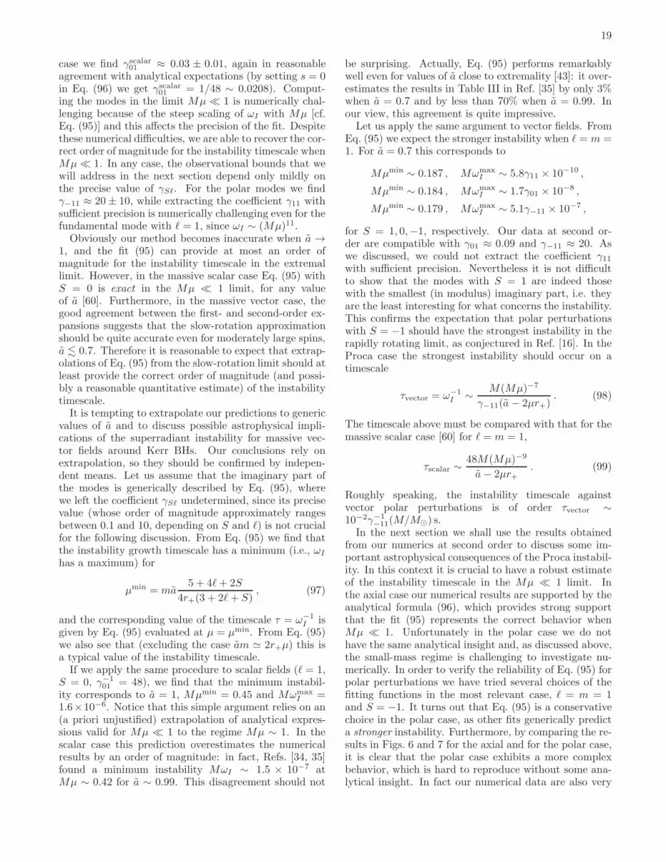
19
case we find γscalar01 ≈ 0.03 ± 0.01, again in reasonableagreement with analytical expectations (by setting s = 0in Eq. (96) we get γscalar01 = 1/48 ∼ 0.0208). Comput-ing the modes in the limit Mµ ≪ 1 is numerically chal-lenging because of the steep scaling of ωI with Mµ [cf.Eq. (95)] and this affects the precision of the fit. Despitethese numerical difficulties, we are able to recover the cor-rect order of magnitude for the instability timescale whenMµ≪ 1. In any case, the observational bounds that wewill address in the next section depend only mildly onthe precise value of γSℓ. For the polar modes we findγ−11 ≈ 20± 10, while extracting the coefficient γ11 withsufficient precision is numerically challenging even for thefundamental mode with ℓ = 1, since ωI ∼ (Mµ)11.Obviously our method becomes inaccurate when a →
1, and the fit (95) can provide at most an order ofmagnitude for the instability timescale in the extremallimit. However, in the massive scalar case Eq. (95) withS = 0 is exact in the Mµ ≪ 1 limit, for any valueof a [60]. Furthermore, in the massive vector case, thegood agreement between the first- and second-order ex-pansions suggests that the slow-rotation approximationshould be quite accurate even for moderately large spins,a . 0.7. Therefore it is reasonable to expect that extrap-olations of Eq. (95) from the slow-rotation limit should atleast provide the correct order of magnitude (and possi-bly a reasonable quantitative estimate) of the instabilitytimescale.It is tempting to extrapolate our predictions to generic
values of a and to discuss possible astrophysical impli-cations of the superradiant instability for massive vec-tor fields around Kerr BHs. Our conclusions rely onextrapolation, so they should be confirmed by indepen-dent means. Let us assume that the imaginary part ofthe modes is generically described by Eq. (95), wherewe left the coefficient γSℓ undetermined, since its precisevalue (whose order of magnitude approximately rangesbetween 0.1 and 10, depending on S and ℓ) is not crucialfor the following discussion. From Eq. (95) we find thatthe instability growth timescale has a minimum (i.e., ωI
has a maximum) for
µmin = ma5 + 4ℓ+ 2S
4r+(3 + 2ℓ+ S), (97)
and the corresponding value of the timescale τ = ω−1I is
given by Eq. (95) evaluated at µ = µmin. From Eq. (95)we also see that (excluding the case am ≃ 2r+µ) this isa typical value of the instability timescale.If we apply the same procedure to scalar fields (ℓ = 1,
S = 0, γ−101 = 48), we find that the minimum instabil-
ity corresponds to a = 1, Mµmin = 0.45 and MωmaxI =
1.6×10⁻⁶. Notice that this simple argument relies on an(a priori unjustified) extrapolation of analytical expres-sions valid for Mµ ≪ 1 to the regime Mµ ∼ 1. In thescalar case this prediction overestimates the numericalresults by an order of magnitude: in fact, Refs. [34, 35]found a minimum instability MωI ∼ 1.5 × 10⁻⁷ atMµ ∼ 0.42 for a ∼ 0.99. This disagreement should not
be surprising. Actually, Eq. (95) performs remarkablywell even for values of a close to extremality [43]: it over-estimates the results in Table III in Ref. [35] by only 3%when a = 0.7 and by less than 70% when a = 0.99. Inour view, this agreement is quite impressive.Let us apply the same argument to vector fields. From
Eq. (95) we expect the stronger instability when ℓ = m =1. For a = 0.7 this corresponds to
Mµmin ∼ 0.187 , MωmaxI ∼ 5.8γ11 × 10−10 ,
Mµmin ∼ 0.184 , MωmaxI ∼ 1.7γ01 × 10−8 ,
Mµmin ∼ 0.179 , MωmaxI ∼ 5.1γ−11 × 10−7 ,
for S = 1, 0,−1, respectively. Our data at second or-der are compatible with γ01 ≈ 0.09 and γ−11 ≈ 20. Aswe discussed, we could not extract the coefficient γ11with sufficient precision. Nevertheless it is not difficultto show that the modes with S = 1 are indeed thosewith the smallest (in modulus) imaginary part, i.e. theyare the least interesting for what concerns the instability.This confirms the expectation that polar perturbationswith S = −1 should have the strongest instability in therapidly rotating limit, as conjectured in Ref. [16]. In theProca case the strongest instability should occur on atimescale
τvector = ω−1I ∼ M(Mµ)−7
γ−11(a− 2µr+). (98)
The timescale above must be compared with that for themassive scalar case [60] for ℓ = m = 1,
τscalar ∼48M(Mµ)−9
a− 2µr+. (99)
Roughly speaking, the instability timescale againstvector polar perturbations is of order τvector ∼10−2γ−1
−11(M/M⊙) s.In the next section we shall use the results obtained
from our numerics at second order to discuss some im-portant astrophysical consequences of the Proca instabil-ity. In this context it is crucial to have a robust estimateof the instability timescale in the Mµ ≪ 1 limit. Inthe axial case our numerical results are supported by theanalytical formula (96), which provides strong supportthat the fit (95) represents the correct behavior whenMµ ≪ 1. Unfortunately in the polar case we do nothave the same analytical insight and, as discussed above,the small-mass regime is challenging to investigate nu-merically. In order to verify the reliability of Eq. (95) forpolar perturbations we have tried several choices of thefitting functions in the most relevant case, ℓ = m = 1and S = −1. It turns out that Eq. (95) is a conservativechoice in the polar case, as other fits generically predicta stronger instability. Furthermore, by comparing the re-sults in Figs. 6 and 7 for the axial and for the polar case,it is clear that the polar case exhibits a more complexbehavior, which is hard to reproduce without some ana-lytical insight. In fact our numerical data are also very

20
well reproduced by the following fitting function:
MωI ∼ (a− aSR) [η0(Mµ)κ0 + η1a(Mµ)κ1 ] , (100)
where
aSR =−m+
√
m2 + 16(Mµ)2
2µM∼ 4Mµ
m+O(µ3) , (101)
corresponding to the superradiance threshold [Eq. (94)]when ωR ∼ µ. The fit (100) has been obtained by im-posing a second-order (in a) functional form and ωI = 0when a = aSR, consistently with our data. Finally, thefunctional dependence on µ of the two remaining termshas been obtained by fitting the data in the instabilityregion and for 0.03 .Mµ . 0.1. We found η0 ≈ −6.5±2,η1 ≈ 2.1 ± 1, κ0 ≈ 6.0 ± 0.1 and κ1 ≈ 5.0 ± 0.3. Whilethe fit (95) is physically more appealing [16], Eq. (100)reproduces our numerical data in the whole instabilityregion within a factor of two. It would be interesting tobetter understand the behavior of the polar instabilityin the limit Mµ ≪ 1 using different approaches, suchas a time-evolution analysis or a full numerical evolutionof the Proca equation. In the following we shall discusshow the choice of either Eq. (95) or Eq. (100) affects theastrophysical implications of our results.
VII. ASTROPHYSICAL IMPLICATIONS OF
THE PROCA INSTABILITY
Our numerical results in the previous section indicatethat polar perturbations with S = −1 have the shortestinstability timescale, as conjectured in [16]. For fixed val-ues of a and µ, the instability timescale for polar pertur-bations is smaller by two-three orders of magnitude thanin the axial case. While this conclusion relies on an ex-trapolation of calculations that are valid (strictly speak-ing) only in the slow-rotation limit, we have shown thata similar extrapolation in the scalar case is in remark-able quantitative agreement with numerical results thatdo not rely on the slow rotation approximation. Further-more, in the Proca case a second-order calculation givessolid evidence that our extrapolation is reliable, bothqualitatively and quantitatively. Therefore it is reason-able to expect that extrapolations from the slow-rotationlimit should at least provide the correct order of magni-tude (and possibly a reliable quantitative estimate) of thepolar instability timescale. Here we explore the tantaliz-ing astrophysical implications of the Proca superradiantinstability. Unless otherwise stated, we shall focus onthe most relevant modes, those with ℓ = m = 1, whichcorrespond to the stronger instability.
A. Implications from the existence of supermassive
black holes
The most conservative assumption on the final state ofthe instability is that the radiation will extract angular
momentum from the BH, leaving behind a Kerr metricwith dimensionless spin parameter below the superradi-ant threshold: in other words, the angular frequency ofthe BH horizon must be such that ΩH . µ. By thisargument, even a single reliable supermassive BH spinmeasurement can impose a stringent constraint on theallowed mass range of massive vector fields. Bounds onthe mass of the vector field follow from the requirementthat astrophysical spinning BHs should be stable, in thesense that the timescale (98) should be larger than someobservational threshold.
0 0.2 0.4 0.6 0.8 1J/M
2
10-20
10-19
10-18
10-17
mv [e
V]
τ = τHubble
τ > τHubble
Unstable
µ=ΩHStable
τ = τSalpeter
τ =104yr
polar S=-1, fit I
FIG. 8. (color online) Bounds on the photon mass mv = ~µobtained by extrapolating the instability timescale (98) forS = −1 polar Proca modes of a Kerr BHs up to a = 1.The region delimited by the curves corresponds to an insta-bility timescale τ < τHubble (continuous red line), τ < τSalpeter(dashed green line) and τ < 104 yr (dot-dashed blue line), re-spectively. We set γ−11 ≈ 20 ± 10 in Eq. (98) and considera Kerr BH with M = 107M⊙, but the results have a simplescaling with γ−11 and with the BH mass (cf. Eqs. (102) and(103)). Thin dashed lines bracket our estimated numericalerrors.
For isolated BHs we can consider the observationalthreshold to be the age of the Universe, τHubble =1.38 × 10¹⁰ yr. A more conservative assumption is toinclude possible spin growth due to mergers with otherBHs and/or accretion. These effects are in competitionwith superradiant angular momentum extraction.The most likely mechanism to produce fast-spinning
BHs3 is prolonged accretion [78]. In this case we cancompare the superradiance timescale to the shortest
3 Supermassive BHs with moderate spin (say a ∼ 0.7, as in Fairall9 [57]) could also be produced by comparable-mass BH merg-ers [9]. The timescale for mergers depends on details of the“final parsec problem”, which are poorly known [75]. The mini-
mum timescale necessary for BHs to merge is the gravitational-radiation timescale, which is of the same order as the Salpetertimescale (cf. Eq. (10) in [75] or Eq. (26) in [76]), but it is likelythat the timescale for binary BHs to merge will be dominated by

21
10-21
10-20
10-19
10-18
10-17
mv [eV]
100
101
102
103
104
105
106
107
108
109
1010
τ [
yr]
MCG-6-30-15Fairall 9SWIFT J2127.4+56541H0707-495Mrk 79Mrk 335NGC 7469NGC 3783
Axial (S=0)
τSalpeter
10-21
10-20
10-19
10-18
10-17
mv [eV]
10-4
10-3
10-2
10-1
100
101
102
103
104
105
106
107
108
109
1010
τ [
yr]
MCG-6-30-15Fairall 9SWIFT J2127.4+56541H0707-495Mrk 79Mrk 335NGC 7469NGC 3783
Polar (S=-1, fit I)
τSalpeter
10-21
10-20
10-19
10-18
10-17
mv [eV]
10-3
10-2
10-1
100
101
102
103
104
105
106
107
108
109
1010
τ [
yr]
MCG-6-30-15Fairall 9SWIFT J2127.4+56541H0707-495Mrk 79Mrk 335NGC 7469NGC 3783
Polar (fit II)
τSalpeter
FIG. 9. (color online) Instability timescale (in years) as a function of the vector mass mv (in eV) for the eight supermassiveBHs listed in Table 2 of [56]. The left panel refers to the axial case (S = 0, ℓ = m = 1); the middle panel to the polar case,Eq. (95) with S = −1, ℓ = m = 1 and γ−11 ≈ 20; the right panel to the polar case, but using the alternative fitting functiongiven in Eq. (100). The horizontal line corresponds to τ = τSalpeter = 4.5× 10⁷ yr.
timescale over which accretion could spin up the BH.Thin-disk accretion can increase the BH spin from a = 0to a ≈ 1 with a corresponding mass increase by a factor√6 [79]. If we assume that mass growth occurs via accre-
tion at the Eddington limit, so that the BH mass growsexponentially with e-folding time given by the Salpetertimescale τSalpeter = 4.5 × 10⁷ yr, then the minimum
timescale for the BH spin to grow from a = 0 to a ≈ 1 viathin-disk accretion is comparable to τSalpeter. Note thataccretion at the Eddington limit is a rather conservativeassumption, since more typically we would expect ac-cretion to be sub-Eddington. Furthermore fast-spinningBHs are hard to produce in the presence of radiative ef-fects [80] or magnetohydrodynamics [81], and “chaotic”accretion [82] would make large spin parameters even lesslikely.
For illustration, in Fig. 8 we consider a Kerr BH withM = 107M⊙, so that mv = 10−17(Mµ) eV. We assumeγ−11 ≈ 20± 10 in Eq. (98) (consistently with our numer-ical results) and we plot: (i) the superradiant threshold(dashed black line), corresponding to the points whereµ ≈ ΩH and the instability timescale (in the perturba-tive treatment) becomes infinite; (ii) the contours cor-responding to an instability timescale τ = τHubble (con-tinuous red line), τ = τSalpeter (dashed green line) andτ = 104 yr (dash-dotted blue line), respectively. Eachcurve is shown with the corresponding error bars.
In the region delimited by the continuous red line theinstability timescale is shorter than the Hubble time(of course, similar considerations apply to the dashedgreen and dash-dotted blue lines). For large a the lowerbranches of the “critical” curves are roughly horizontal.By solving ω−1
I = τc in the limit Mµ ≪ 1 this regime
the dynamical friction timescale, which is typically of the orderof a few Gyrs for satellites in a Milky Way-type halo [77] andhence larger than the Salpeter timescale.
can be well approximated by the formula
m∗v = ~µ∗ =
~
M
[
M
mγSℓτc
]1/(5+4ℓ+2S)
, (102)
where τc is the threshold time. If τc = τHubble and in theS = −1 polar case, we get
m∗v ∼ 7× 10⁻²⁰
γ1/7−11
[
107M⊙
M
]6/7
eV . (103)
Note that, although extracting the values of the fittingparameters can be numerically challenging, our resultsdepend very mildly on the precise value of γ−11. FromEq. (98) we see that the instability timescale is inverselyproportional to γ−11. Therefore the near-horizontal “ob-servability threshold” in Fig. 9 that would correspond tochoosing τ = τSalpeter rather than τ = τHubble can beobtained multiplying γ−11 in Eq. (103) by the ratio ofthe two timescales, τSalpeter/τHubble ≃ 3 × 10⁻³. Thenthe vector mass bound (103) would increase by a mod-est factor of 2.3. What is crucial in obtaining strongastrophysical bounds is having a large BH mass, because
bounds scale like(
107M⊙/M)6/7
.Brenneman et al. [56] have recently presented a list
of eight supermassive BH mass and spin estimates. InFig. 9 we show the superradiant instability timescale τ(in years) as a function ofmv (in eV) for these supermas-sive BHs. The dashed horizontal line denotes τSalpeter,which we (conservatively) assume as the threshold forthe timescale to be observationally significant. For eachsystem we compute instability timescales using the BHmass and spin estimates given in Table 2 of [56] (we se-lect either the average spin value quoted in the table, orthe lower limit on the spin when the observations im-ply a > 0.98). The left panel refers to axial modes withS = 0 and ℓ = m = 1, for which we can compute theinstability timescale analytically: cf. Eq. (96) and Ap-pendix C. The middle and right panels shows that quali-tatively similar results hold for polar modes with S = −1and ℓ = m = 1, which exhibit the strongest instability.

22
In the polar case, we computed the instability timescaleusing both Eq. (95) (fit I) and Eq. (100) (fit II). Theresults are qualitatively similar and show that, indepen-dently of the fitting function, the axial bounds on mv
are typically one-two orders of magnitude less stringentthan the polar bounds. Fig. 9 shows that existing mea-surements of supermassive BH spins rule out Proca fieldmasses in the whole range 10−20 eV. mv . 10−17 eV.Note that arguments based on the superradiant insta-
bility can only be used to set “exclusion windows” on theboson mass, rather then upper bounds [42, 43]. How-ever, observations of BHs in different mass ranges canexclude different mass windows. For example, stellar-size BHs, M ≃ (5 − 20)M⊙, can set an exclusion regionof 10−13 eV. mv . 10−9 eV. This mass range is relevantfor so-called “dark photons” coupled to sterile neutri-nos [83]. If the identified intermediate-mass BHs wereconfirmed to exist and if the largest known supermas-sive BHs with M ≃ 2 × 10¹⁰M⊙ [84, 85] were confirmedto have sufficiently large spin, combined observations ofspinning BHs can potentially exclude the entire masswindows 10−21 eV. mv . 10−9 eV [42, 43]. The lat-ter is complementary to the bounds set by several otherexperiments and observations that exclude light bosonicparticle with larger mass [52, 83, 86].Using current data on supermassive BHs [56], the best
bound comes from Fairall 9 [57], for which the polar in-stability implies a conservative bound (including mea-surement errors) mv . 10−20 eV or mv . 10−21 eV,depending on the fitting function [59]. Although the in-stability for axial modes is weaker, in this case our re-sults are more precise and imply a bound as stringentas mv . 4 × 10⁻²⁰ eV if we consider τ < τSalpeter, ormv×10−20 eV if we consider τ < τHubble. Even under ourvery conservative assumptions these results are of greatsignificance, since the current best bound on the photonmass ismγ < 10−18 eV [52, 86]. Combining the exclusionwindow derived above, 10−20 . mv . 10−17 eV, with ex-isting bounds [52, 86], we find the most stringent upperbound on the photon mass, mγ . 10−20 eV.We remind the reader that our results are also sum-
marized in Fig. 1, where we show instability windows foraxial and polar modes together with supermassive BHmass and spin estimates from Ref. [56].
B. Nonlinear effects, other couplings
An important ingredient that was not taken into ac-count in our study is the nonlinear evolution of the insta-bility, that can modify the background geometry. Photonself-interactions are very weak, being suppressed by themass of the electron. Therefore, it is quite likely thatthe outcome of the instability will be a slow and gradualdrainage of the hole’s rotational energy. However, exoticmassive vector fields may show nonlinearities as thosestudied in Ref. [46, 47] for the scalar case.Another important aspect that should be investigated
is whether the coupling of accreting matter to massivebosons can quench the instability. In principle massivephotons (unlike hidden U(1) fields, for which the inter-action with matter is very small) can couple strongly tomatter. However it is unlikely that this will significantlyaffect the superradiant instability discussed here, for tworeasons. The first is that unstable modes are large-scalecoherent modes whose Compton wavelength is compara-ble to (or larger than) the size of the BH’s event hori-zon, and accretion disks are typically charge-neutral overthese lengthscales, so any possible coupling with ordinaryneutral matter is incoherent and most likely inefficient.The second is that accretion disks are expected to belocalized on the equatorial plane, and therefore can af-fect at most some (but not all) of the unstable modes.The investigation of the superradiant instability in thepresence of matter requires further work, but the aboveconsiderations suggest that vacuum estimates should bereliable. Spin estimates for slowly accreting BHs (suchas the BH at the center of our own galaxy) are the mostreliable, in that they should be less sensitive to details ofthe interaction of vector fields with matter.
VIII. CONCLUSIONS AND EXTENSIONS
BH perturbation theory is a powerful tool, with impor-tant applications in astrophysics and high-energy physics,but its applicability is limited when the perturbationequations cannot be separated. We have discussed a gen-eral method to circumvent these difficulties in the case ofslowly rotating BH spacetimes. The method was origi-nally developed to study the modes of rotating stars but,as we showed, it applies to any slowly rotating BH back-ground and to any kind of perturbation. Within this gen-eral framework, we discussed two effects induced by ro-tation: (i) the Zeeman-like splitting of the eigenfrequen-cies, that breaks the degeneracy of modes with differentazimuthal number m, and (ii) a Laporte-like selectionrule, in which modes with multipolar index ℓ are coupledto those with multipolar index ℓ± 1 and opposite parityand to those with ℓ ± 2 and same parity. We have ex-tended Kojima’s arguments to show that these couplingsdo not affect the QNM frequencies of the spacetime tofirst order in the rotation rate, and we verified this claimby numerical integration of the perturbation equations.As a first relevant application of this method, we stud-
ied massive vector (Proca) perturbations on a slowly ro-tating Kerr background, i.e. the only interesting classof perturbations of Kerr BHs in four dimensions thatdoes not seem to be separable. Using our approach wereduced the equations to a set of coupled ODEs, thatcan be solved by a straightforward extension of methodsvalid in the nonrotating case. We have computed thecorrections to the Proca eigenfrequencies of a Kerr BHto first and to second order in the rotation rate. For thefirst time we showed that the Proca bound-state modesbecome unstable when the superradiant condition (74)

23
is met. We proved this numerically for the polar modes,and both numerically and analytically for the axial modesin the limitMµ≪ 1. Unfortunately the method becomesintrinsically inaccurate for large values of the rotationrate. This prevents us from accurately computing theinstability timescale close to extremality. By fitting andextrapolating our data we confirmed the scaling with mv
conjectured in Ref. [16], and we also estimated the orderof magnitude of the instability timescale. We expect ourresults to be reliable up to a ∼ 0.7. Our estimates shouldbe confirmed by more accurate methods, but they pro-vide strong evidence that measurements of rotating su-permassive BH spins set the most stringent upper boundson the photon mass (cf. Fig. 1).
Besides their astrophysical implications, our results arerelevant also for some classes of gravitational theorieswith higher-order curvature terms in the action. Forexample, as proved by Buchdahl [87], a theory definedby L =
√−g(
R+ αR[ab]R[ab]
)
in the Palatini approachis dynamically equivalent to the Einstein-Proca systemwhen the vector mass µ2 = 3/|α| (see also Ref. [88]).The Proca instability of Kerr BHs in this theory can putconstraints on the parameter α, which is related to thenonmetricity of the connection.
While limited by the slow-rotation assumption, thepower of the present method consists in its generality.The slow-rotation approximation allows us to study lin-ear perturbations of any slowly rotating spacetime evenwhen the equations are nonseparable. For instance itcan be used to study gravitational-electromagnetic per-turbations of Kerr-Newman BHs in four dimensions [12],QNMs of Myers-Perry BHs [14] and BH greybody fac-tors in higher-dimensional rotating spacetimes [11, 54].Another interesting extension is the stability analysis ofrotating BHs in asymptotically anti-de Sitter spacetimes.This is relevant in the context of the gauge/gravity du-ality, as the QNMs of anti-de Sitter BHs in five dimen-sions are holographically related to specific correlationfunctions and transport coefficients of the dual bound-ary theory [4].
We note that perturbations of rotating stars have beenstudied up to second order in the Cowling approximation(see e.g. Refs. [89–91]), where metric perturbations areneglected and the equations have a structure reminiscentof our general Eqs. (4) and (5).
Finally we remark that the techniques discussed in thispaper are not limited to general relativity. They are alsouseful to study gravitational perturbations and the lin-ear stability of slowly rotating BH metrics in alterna-tive theories of gravity, for example in quadratic grav-ity [22, 25, 26]. We hope to report on these interestingextensions in the near future.
ACKNOWLEDGMENTS
We wish to thank the Axiverse Project members(especially Hideo Kodama), Antonino Flachi, StefanoLiberati and Joao Rosa for valuable discussions, andthe referees for their constructive comments. Thiswork was supported by the DyBHo–256667 ERC Start-ing Grant, the NRHEP–295189 FP7–PEOPLE–2011–IRSES Grant, and by FCT - Portugal through PTDCprojects FIS/098025/2008, FIS/098032/2008, CTE-ST/098034/2008, CERN/FP/123593/2011. A.I. wassupported by JSPS Grant-in-Aid for Scientific ResearchFund No. 22540299 and No. 22244030. E.B. was sup-ported by NSF Grant No. PHY-0900735 and NSF CA-REER Grant No. PHY-1055103. P.P. acknowledgesfinancial support provided by the European Commu-nity through the Intra-European Marie Curie contractaStronGR-2011-298297 and the kind hospitality of theDepartment of Physics, University of Rome “Sapienza”and of the International School for Advanced Studies(SISSA) in Trieste. V.C. thanks the Yukawa Institutefor Theoretical Physics at Kyoto University for hospital-ity during the YITP-T-11-08 workshop on “Recent ad-vances in numerical and analytical methods for black holedynamics”.
Appendix A: Coefficients of the perturbation
equations
In this Appendix we list the explicit form of the co-efficients appearing in the perturbation equations. We
remark that the coefficients Aℓ, Dℓ, A(i)ℓ , B
(i)ℓ , D
(i)ℓ incor-
porate terms at zeroth, first and second order in the ro-tation parameter a. Therefore, there is no direct corre-spondence between these coefficients and the quantitiesat fixed order in a, such as Aℓ, Aℓ, Aℓ, etc., which havebeen introduced in Sec. II. In the following, a prime de-notes derivative with respect to the radial coordinate r.
1. Coefficients of the scalar equation
The explicit form of the coefficients appearing inEq. (22) is
Aℓ = −2[
M2r2((
4M2 + 2Mr(
Λ− 1 + r2µ2)
+ r4ω2
−r2(
Λ + r2µ2))
Ψℓ + r(r − 2M) (2MΨ′ℓ
+r(r − 2M)Ψ′′ℓ ))] + 8amM4r3ωΨℓ + a2M4
[(
36M2
+2Mr(
Λ − 11 + r2µ2)
− r2(
Λ− 2 + 2m2 + r2µ2)
+r3ω2
r − 2M
(
8M2 − 2Mr + r2)
)
Ψℓ
+r(r − 2M) (10MΨ′ℓ − r(2M + r)Ψ′′
ℓ )] , (A1)
Dℓ = 2a2M4[(
4M2 − Λr2 + 2Mr(
Λ− 1 + r2ω2))
Ψℓ
+r(r − 2M) (2MΨ′ℓ + r(r − 2M)Ψ′′
ℓ )] . (A2)

24
2. Coefficients of the Proca perturbation equations
In this Appendix we list the coefficients appearing in Eqs. (44)–(47). The coefficients read
A(0)ℓ =
a2M2
2r6
[
uℓ(1)(
−r2(
Λ + 2m2 + µ2r2 − 2)
+ 32M2 + 2Mr(
Λ + µ2r2 − 10))
2M − r+
r
ℓ(ℓ+ 1)(r − 2M)2
(
(2M − r)(
ℓ(ℓ+ 1)(2M − r)(
−12Mu′ℓ(1) + r(2M + r)u′′
ℓ(1) + ir2ωu′
ℓ(2)
)
− 2im2r2ωuℓ(3)
)
−iΛrω(
−8M2 − 2Mr + r2)
uℓ(2)
)]
+2amM2
(
Λrωuℓ(1) − i(
(2M − r)u′ℓ(3) − r2ω2uℓ(3) + Λuℓ(2)
))
Λr4(2M − r)
−(2M − r)
(
Λ + µ2r2)
uℓ(1) + r(r − 2M)2u′′ℓ(1) + irω
(
(2M − r)(
uℓ(3) − ru′ℓ(2)
)
+ (r − 4M)uℓ(2)
)
r3(2M − r), (A3)
A(1)ℓ =
a2M2
2Λr4(2M − r)3
[
Λuℓ(2)(
(2M − r)(
ℓ2(2M + r) + ℓ(2M + r) + r(
2m2 + µ2r(2M + r)))
+ r2ω2(
8M2 + 2Mr + r2))
+2m2r(r − 2M)2u′ℓ(3) + iΛrω(2M − r)
(
8M2 − 2Mr + r2)
u′ℓ(1) − iℓ(ℓ+ 1)ω(2M − r)
(
8M2 − 6Mr + 3r2)
uℓ(1)
]
+2amM2
(
r2ω(r − 2M)u′ℓ(3) + iΛ
(
(2M − r)uℓ(1) + r(
(r − 2M)u′ℓ(1) + 2irωuℓ(2)
)))
ℓ(ℓ+ 1)r4(r − 2M)2
+(2M − r)
(
(2M − r)u′ℓ(3) + ir2ωu′
ℓ(1)
)
+ uℓ(2)(
(2M − r)(
Λ + µ2r2)
+ r3ω2)
− irω(2M − r)uℓ(1)
r2(r − 2M)2, (A4)
A(2)ℓ =
a2M2(
(2M − r)(
−2m2ruℓ(3) − Λr(r − 2M)u′ℓ(2) − Λ(2M − r)uℓ(2)
)
− iΛrω(
8M2 − 2Mr + r2)
uℓ(1)
)
ℓ(ℓ+ 1)(r − 2M)2
+4amM2r(rωuℓ(3) + iΛuℓ(1))
Λ(2M − r)+
2r2(
(2M − r)(
ru′ℓ(2) + uℓ(2) − u(3)
ℓ(r))
− ir2ωuℓ(1)
)
2M − r, (A5)
A(0)ℓ =
4aM2uℓ(4)
r5−
4a2mM3ωuℓ(4)
Λr5, (A6)
A(1)ℓ = −
2ia2mM2u′ℓ(4)
Λr4, (A7)
A(2)ℓ = 0 , (A8)
B(0)ℓ =
a2mM2ωuℓ(4)
ℓ(ℓ+ 1)r3(2M − r)−
2aM2(
(r − 2M)u′ℓ(4) + r2ω2uℓ(4)
)
Λr4(2M − r), (A9)
B(1)ℓ =
ia2mM2u′ℓ(4)
ℓ(ℓ+ 1)r3(2M − r)−
2iaM2ωu′ℓ(4)
Λr2(2M − r), (A10)
B(2)ℓ =
2ia2mM2ruℓ(4)
Λ(r − 2M)−
4iaM2r2ωuℓ(4)
Λ(r − 2M), (A11)
B(0)ℓ =
4a2M3(Λuℓ(1) + irωuℓ(3))
ℓ(ℓ+ 1)r6, (A12)
B(1)ℓ =
2a2M2(
(r − 2M)u′ℓ(3) − Λuℓ(2)
)
Λr4(2M − r), (A13)
B(2)ℓ = 0 , (A14)

25
D(0)ℓ =
a2M2
r6(2M − r)
[
−(2M − r)(6M − Λr)uℓ(1) + r(
(2M − r)(
6Mu′ℓ(1) − r(r − 2M)u′′
ℓ(1) + irω
(
uℓ(3) − ru′ℓ(2)
))
−irω(10M − r)uℓ(2)
)]
, (A15)
D(1)ℓ =
a2M2
r4(r − 2M)2
[
uℓ(2)(
−ℓ(ℓ+ 1)(2M − r)− 2Mr2ω2)
+ (2M − r)(
(r − 2M)u′ℓ(3) − 2iMrωu′
ℓ(1)
)
+ 2iMω(2M − r)uℓ(1)
]
,
(A16)
D(2)ℓ =
2a2M2
2M − r
[
−(2M − r)(
ru′ℓ(2) + uℓ(2) − u(3)
ℓ(r))
+ 2iMrωuℓ(1)
]
, (A17)
and
αℓ =a2M2
2Λr4(r − 2M)2
[
−48M3u′ℓ(3) + 4M2rℓ2u′
ℓ(2) + 4ℓM2ru′
ℓ(2) + 48M2ru′
ℓ(3) − 4Mr3ω2uℓ(3) + iΛr2ω(2M + r)uℓ(1)
−4Mr2ℓ2u′ℓ(2) − 4ℓMr2u′
ℓ(2) − 12Mr2u′
ℓ(3) − 3Λ(r − 2M)2uℓ(2) + 4Mr(r − 2M)2u′′
ℓ(3) + r3ℓ2u′
ℓ(2) + ℓr3u′
ℓ(2)
]
+2amM2(rωuℓ(3) − iΛuℓ(1))
ℓ(ℓ+ 1)r3(2M − r)+
1
Λr2(2M − r)
[
4M2u′ℓ(3) − 2µ2Mr2uℓ(3) − 2Mrℓ2u′
ℓ(2) − 2ℓMru′
ℓ(2) + Λ(2M − r)uℓ(2)
−2Mru′ℓ(3) − r(r − 2M)2u′′
ℓ(3) + µ2r3uℓ(3) − r3ω2uℓ(3) + iΛr2ωuℓ(1) + r2ℓ2u′
ℓ(2) + ℓr2u′
ℓ(2)
]
, (A18)
βℓ =a2M2
(
−uℓ(4)(
ℓ(ℓ+ 1)(r − 2M)2 − 2Mr3ω2)
− 2M(r − 2M)2(
ru′′ℓ(4) − 3u′
ℓ(4)
))
Λr4(r − 2M)2−
2amM2ωuℓ(4)
Λr2(2M − r)
+uℓ(4)
(
(2M − r)(
Λ + µ2r2)
+ r3ω2)
+ (2M − r)(
r(2M − r)u′′ℓ(4) − 2Mu′
ℓ(4)
)
Λr2(2M − r), (A19)
ζℓ = −a2mM2
(
2ΛMrωuℓ(1) − i(
−2Mr2ω2uℓ(3) + (r − 2M)(
−8Mu′ℓ(3) − r(r − 2M)u′′
ℓ(3) + Λru′
ℓ(2)
)
+ Λ(8M − r)uℓ(2)
))
Λr4(2M − r)
−6aM2
(
(2M − r)uℓ(1) + r(
(r − 2M)u′ℓ(1) + irωuℓ(2)
))
r4(2M − r), (A20)
ηℓ =2iaM2ωuℓ(4)
2Mr2 − r3−ia2mM2
(
−2(
6M2 − 5Mr + r2)
u′ℓ(4) + 2M
(
Λ + r2ω2)
uℓ(4) + r(r − 2M)2u′′ℓ(4)
)
Λr4(2M − r), (A21)
ρℓ =a2M2
Λr4(2M − r)
[
12M2u′ℓ(3) − 2Mr2ω2uℓ(3) + 2iΛMrωuℓ(1) − 2Mrℓ2u′
ℓ(2) − 2ℓMru′
ℓ(2) + 3Λ(2M − r)uℓ(2)
−10Mru′ℓ(3) − r(r − 2M)2u′′
ℓ(3) + r2ℓ2u′
ℓ(2) + ℓr2u′
ℓ(2) + 2r2u′
ℓ(3)
]
, (A22)
λℓ = −4a2M3uℓ(4)
r5, (A23)
σℓ = 0 , (A24)
γℓ =a2M2
Λr4(2M − r)
[
uℓ(4)(
ℓ(ℓ+ 1)(2M − r) + 2Mr2ω2)
+ (2M − r)(
r(2M − r)u′′ℓ(4) − 8Mu′
ℓ(4)
)]
. (A25)
(A26)
Appendix B: Proca equation for a slowly rotating
Kerr BH
In this Appendix we list the perturbation equationsfor a Proca field on a slowly rotating Kerr background to
first order in a. Equation (55) reads
D2uℓ(4) −
4aM2mω
r3uℓ(4)
=6aM2
r4
[
(ℓ+ 1)Qℓ
(
Fuℓ−1(1) − i rωuℓ−1
(2) − Fru′ℓ−1(1)
)
+ℓQℓ+1
(
i rωuℓ+1(2) − Fuℓ+1
(1) + Fru′ℓ+1(1)
)]
, (B1)

26
where the operator D2 is defined in Eq. (24). The Lorenzcondition (Eq. (53) with I = 2) becomes
i rωuℓ(1) + F(
uℓ(2) − uℓ(3) + ru′ℓ(2)
)
− 2aM2m
r2
(
iuℓ(1) +rω
Λuℓ(3)
)
=2i aM2ω
rΛ
[
(ℓ+ 1)Qℓuℓ−1(4) − ℓQℓ+1u
ℓ+1(4)
]
. (B2)
Using Eq. (B2), Eqs. (53) with I = 0, 1 and Eq. (54) read
D2uℓ(3) +
2Fℓ(ℓ+ 1)
r2uℓ(2) +
2aM2m
r4
[
rω(3uℓ(2) − 2uℓ(3))
+3iF(
uℓ(1) − ru′ℓ(1)
)]
= 0 , (B3)
D2uℓ(2) −
2F
r2
(
1− 3M
r
)
[
uℓ(2) − uℓ(3)
]
− 2aM2m
ℓ(ℓ+ 1)r4
[
ℓ(ℓ+ 1)(2rωuℓ(2) − 3iFuℓ(1))− 3rωFuℓ(3)
]
= −6i aM2Fω
ℓ(ℓ+ 1)r3
[
(ℓ + 1)Qℓuℓ−1(4) − ℓQℓ+1u
ℓ+1(4)
]
, (B4)
D2uℓ(1) −
2M
r2
(
iωuℓ(2) + Fu′ℓ(1)
)
− 2aM2m
ℓ(ℓ+ 1)r4
[
ℓ(ℓ+ 1)(2rωuℓ(1) − iuℓ(2)) + i rFu′ℓ(3)
]
= − 2aM2F
ℓ(ℓ+ 1)r4
[
(ℓ + 1)Qℓ
(
2ℓuℓ−1(4) + ru′
ℓ−1(4)
)
+ℓQℓ+1
(
2(ℓ+ 1)uℓ+1(4) − ru′
ℓ+1(4)
)]
. (B5)
The system (B1), (B3)–(B5) can be greatly simplified by
a systematic use of Eq. (B2) to eliminate uℓ(1) and uℓ±1(1) .
Solving Eq. (B2) for uℓ(1) and substituting in Eq. (B3)–
(B4) we get, to first order in a, the equations listed inthe main text, namely Eqs.(59) and (60).In order to simplify the axial equation (B1), we con-
sider Eq. (B2) with ℓ− 1 and ℓ+ 1 and solve it for uℓ−1(1)
and uℓ+1(1) , respectively. To first order in a, and making
also use of Eq. (59) and (60), we get Eq. (61).
Appendix C: Analytical results for the axial modes
In this appendix we generalize Detweiler’s calcula-tion [60] of the unstable massive scalar modes of a KerrBH to the case of a massive vector field. We focus onthe axial sector and, unlike Detweiler, we work in theslow-rotation limit up to first order in a.As discussed in the main text, the axial vector equa-
tion (65) and the equation for scalar perturbations (66)can be written in a unified form, Eq. (66). Thus, inorder to include both scalar and axial vector perturba-tions, we shall solve Eq. (66) in the Kerr case, whereF = B = 1 − 2M/r and = 2aM2/r. By defining
R(r) = Ψ/r we get
r2Fd
dr
(
r2FdR
dr
)
+[
r4ω2 − 4amrω
−r2F(
ℓ(ℓ+ 1) + µ2r2 − 2Ms2
r
)]
R = 0 . (C1)
For s = 0, the equation above is equivalent to Eq. (7)in Ref. [60] at first order. For s = ±1 and a = 0 it isequivalent to Eq. (51) in Ref. [16].Following Starobinski’s method of matching asymp-
totics [92], we first expand Eq. (C1) for r ≫M :
d2(rR)
dr2
[
ω2 − µ2 +2Mµ2
r− ℓ(ℓ+ 1)
r2
]
rR = 0 . (C2)
The solution of this equation with the correct boundarycondition at infinity reads
R∞(x) ∝ xℓe−x/2U(ℓ+ 1− ν, 2ℓ+ 2, x) , (C3)
where U(p, q, x) is one of the confluent hypergeomet-ric functions [93], x = 2k∞r, k2∞ = µ2 − ω2 andν = Mµ2/k∞. The small distance (x ≪ 1) behaviorof the solution above reads
R∞(r) ∼ (−1)n(2ℓ+ 1 + n)!
(2ℓ+ 1)!(2k∞r)
ℓ
+ (−1)n+1δν(2ℓ)!(2k∞r)−ℓ−1 , (C4)
where we have defined δν = ν − ℓ − 1 − n and assumedδν ∼ x2ℓ+1 ≪ 1 [60].On the other hand, Eq. (C1) can be solved analytically
also when r ≪ max(ℓ/ω, ℓ/µ). In this limit, by intro-ducing a new coordinate z = (r − r+)/r+, the equationreduces to
Zd
dz
[
ZdR
dz
]
+[
P 2 − ℓ(ℓ+ 1)Z + s2z]
R = 0 . (C5)
We defined Z = z(z + 1) and
P = −2MkH = −2M(ω −mΩH) , (C6)
and we neglected O(a2) terms in P 2. The general so-lution of Eq. (C5) is a combination of hypergeometricfunctions. By imposing ingoing waves at the horizon, i.e.R ∼ ziP at z ∼ 0, we get the general solution with thecorrect boundary condition:
RH(r)∝ e−2Pπ(−1)2iP ziP ×2F1 [−ℓ+ iP + σ, 1 + ℓ+ iP + σ, 1 + 2iP,−z] ,
where 2F1(a, b, c, z) is the hypergeometric function [93]
and σ =√s2 − P 2. The large-distance limit of the equa-
tion above reads
RH(r) ∼[
(2M)−ℓΓ[1 + 2ℓ]
Γ [1 + ℓ+ iP − σ] Γ [1 + ℓ+ iP + σ]
]
rℓ
+
[
(2M)1+ℓΓ[−1− 2ℓ]
Γ [−ℓ+ iP − σ] Γ [−ℓ+ iP + σ]
]
r−ℓ−1 . (C7)

27
The key point of the method of matching asymptoticsis that, when |Mω| ≪ ℓ and Mµ ≪ ℓ, there exists anoverlapping region where Eqs. (C7) and (C4) are bothvalid. By equating the coefficients of rℓ and r−ℓ−1 onecan fix the ratio of the overall factors and the frequencyof the mode. Finally, we get
δν =(4k∞M)2ℓ+1Γ[−1− 2ℓ]Γ[2 + n+ 2ℓ]
Γ[1 + n]Γ[1 + 2ℓ]2Γ[2 + 2ℓ]×
Γ [1 + iP − σ + ℓ] Γ [1 + iP + σ + ℓ]
Γ [iP − σ − ℓ] Γ [iP + σ − ℓ]. (C8)
As in the case of massive scalar perturbations, the realand imaginary parts of the mode are related to µ and δνby [60]
µ2 − ω2R = µ2
(
Mµ
ℓ+ n+ 1
)2
, (C9)
iωI =δν
M
(
Mµ
ℓ+ n+ 1
)3
. (C10)
In the slow-rotation limit we can further simplifyEq. (C8). To first order in P we get
δν∼ iP (4k∞M)2ℓ+1Γ[2 + 2ℓ+ n]
Γ[1 + 2ℓ]2Γ[2 + 2ℓ]2Γ[1 + n]×
Γ[1 + ℓ− s]Γ[1 + ℓ+ s]Γ[1 + ℓ]2s∏
j=1
[
j − 1− s− ℓ
s− j − ℓ
]
,
(C11)
When s = 0 we recover the result for the scalar case [60]to first order in P (but see the subsection below for adiscussion). In addition, our results correctly reduce tothose found in Ref. [16] in the nonrotating limit. We cannow evaluate the instability timescale. The fundamentalmode reads
Mω(ℓ=1)I =
(s+ 1)!(s+ 1)
48(am− 2r+µ) (Mµ)9 ,
(C12)
Mω(ℓ=2)I =
[(2 − s)!(2 + s)!]2
885735(am− 2r+µ) (Mµ)13 ,
for ℓ = 1 and ℓ = 2, respectively. Note that ωI ∼ µ4ℓ+5
for any value of s, so the only difference arises in the
prefactor. We find
ω(s=±1)I
ω(s=0)I
=(1 + ℓ)2
ℓ2, (C13)
which is independent of µ, a and n. The instabilitytimescale of the ℓ = 1 axial vector mode is 4 times shorterthan that of the scalar mode. Equation (C12) is com-pared to the numerical results in Fig. 5.
On the analytical result in the massive scalar case
Although this is not directly related to the Proca prob-lem, we wish to remark that when s = 0 our equa-tion (C11) differs from Eq. (28) in Ref. [60] (expandedat first order) by a factor 2 for any ℓ and any n. We be-lieve this is either due to an inconsistent limit (explainedbelow) or to a typo in Ref. [60] which propagates fromEqs. (21)-(24) to Eq. (25), where a factor 1/2 is missing.Thus, Eq. (29) in Detweiler should read γ = µa(µM)8/48for consistency with our Eq. (C12).In order to understand the source of this discrep-
ancy we refer the reader to the work by Furuhashi andNambu [94], who extended Detweiler’s calculation to thecase of Kerr-Newman BHs, reproducing the results ofRef. [60] in the zero-charge limit. Ref. [94] presents adetailed derivation of the instability timescale, facilitat-ing intermediate comparisons with our own calculation.We note that the results in Ref. [94] seem to be par-tially flawed because the limit defined in Eq. (23) inRef. [94], Γ(−n)/Γ(−m) = (−1)n−mm!/n!, is valid onlywhen n and m are integers. However, in a rotating back-ground the angular eigenvalues are not (in general) in-tegers. For example, in the scalar case the separationconstant λ = ℓ(ℓ + 1) + O(aMω) [60]. In the Mω ≪ 1limit, this can be accounted for by considering ℓ→ ℓ+ ǫ,with ǫ ≪ 1. When s = 0, the evaluation of Eq. (C8)above involves limits of the form
limǫ→0
Γ(−2ℓ− 2ǫ− 1)
Γ(−ℓ− ǫ)=
(−1)ℓ+1
2
ℓ!
(2ℓ+ 1)!, (C14)
which differs by a factor 2 from Eq. (23) in Ref. [94] (seealso the discussion in Ref. [95]). We believe that this isthe reason for our factor 2 discrepancy with respect toFuruhashi and Nambu (and presumably also with respectto Detweiler’s calculation). Despite numerical difficultiesin the Mµ ≪ 1 limit, our numerical calculations for ℓ =m = 1 are in better agreement with a prefactor of 1/48,as computed in Eq. (C12): see also Sec. VI F and Fig. 6in Ref. [35].
[1] H.-P. Nollert, Class.Quant.Grav. 16, R159 (1999).[2] K. D. Kokkotas and B. G. Schmidt, Living Rev.Rel. 2, 2
(1999), arXiv:gr-qc/9909058 [gr-qc].
[3] V. Ferrari and L. Gualtieri, Gen.Rel.Grav. 40, 945(2008), arXiv:0709.0657 [gr-qc].
[4] E. Berti, V. Cardoso, and A. O. Starinets,

28
Class.Quant.Grav. 26, 163001 (2009), arXiv:0905.2975[gr-qc].
[5] R. Konoplya and A. Zhidenko, Rev.Mod.Phys. 83, 793(2011), arXiv:1102.4014 [gr-qc].
[6] P. Amaro-Seoane, J. R. Gair, M. Freitag, M. Cole-man Miller, I. Mandel, et al., Class.Quant.Grav. 24,R113 (2007), arXiv:astro-ph/0703495 [ASTRO-PH].
[7] L. Barack, Class.Quant.Grav. 26, 213001 (2009),arXiv:0908.1664 [gr-qc].
[8] E. Poisson, A. Pound, and I. Vega, Living Rev.Rel. 14,7 (2011), arXiv:1102.0529 [gr-qc].
[9] E. Berti, V. Cardoso, J. A. Gonzalez, U. Sperhake,M. Hannam, et al., Phys.Rev. D76, 064034 (2007),arXiv:gr-qc/0703053 [GR-QC].
[10] E. Berti, V. Cardoso, T. Hinderer, M. Lemos,F. Pretorius, et al., Phys.Rev. D81, 104048 (2010),arXiv:1003.0812 [gr-qc].
[11] V. Cardoso, L. Gualtieri, C. Herdeiro, U. Sperhake, P. M.Chesler, et al., (2012), arXiv:1201.5118 [hep-th].
[12] S. Chandrasekhar, The mathematical theory of blackholes (Oxford University Press, New York, 1992).
[13] S. A. Teukolsky, Astrophys.J. 185, 635 (1973).[14] M. Durkee and H. S. Reall, Class.Quant.Grav. 28, 035011
(2011), arXiv:1009.0015 [gr-qc].[15] G. Torres del Castillo and G. Silva-Ortigoza, Phys.Rev.
D42, 4082 (1990).[16] J. G. Rosa and S. R. Dolan, Phys.Rev. D85, 044043
(2012), arXiv:1110.4494 [hep-th].[17] Y. Kojima, Phys.Rev. D46, 4289 (1992).[18] Y. Kojima, Astrophys.J. 414, 247 (1993).[19] Y. Kojima, Progress of Theoretical Physics 90, 977
(1993).[20] M. Bruni, L. Gualtieri, and C. F. Sopuerta,
Class.Quant.Grav. 20, 535 (2003), arXiv:gr-qc/0207105[gr-qc].
[21] S. Chandrasekhar and V. Ferrari, Proc.Roy.Soc.Lond.A433, 423 (1991).
[22] N. Yunes and F. Pretorius, Phys.Rev. D79, 084043(2009), arXiv:0902.4669 [gr-qc].
[23] K. Konno, T. Matsuyama, and S. Tanda,Prog.Theor.Phys. 122, 561 (2009), arXiv:0902.4767[gr-qc].
[24] P. Pani and V. Cardoso, Phys.Rev. D79, 084031 (2009),arXiv:0902.1569 [gr-qc].
[25] P. Pani, C. F. Macedo, L. C. Crispino, and V. Cardoso,Phys.Rev. D84, 087501 (2011), arXiv:1109.3996 [gr-qc].
[26] K. Yagi, N. Yunes, and T. Tanaka, Phys.Rev. D86,044037 (2012), arXiv:1206.6130 [gr-qc].
[27] N. Andersson, Astrophys.J. 502, 708 (1998),arXiv:gr-qc/9706075 [gr-qc].
[28] Y. Kojima, Mon.Not.Roy.Astron.Soc. 293, 49 (1998),arXiv:gr-qc/9709003 [gr-qc].
[29] K. H. Lockitch and J. L. Friedman, Astrophys.J. 521,764 (1999), arXiv:gr-qc/9812019 [gr-qc].
[30] K. H. Lockitch, N. Andersson, and J. L. Friedman,Phys.Rev. D63, 024019 (2001), arXiv:gr-qc/0008019[gr-qc].
[31] W. H. Press and S. A. Teukolsky, Nature 238, 211 (1972).[32] T. Damour, N. Deruelle, and R. Ruffini, Lett.Nuovo
Cim. 15, 257 (1976).[33] V. Cardoso, O. J. Dias, J. P. Lemos, and S. Yoshida,
Phys.Rev. D70, 044039 (2004), arXiv:hep-th/0404096[hep-th].
[34] V. Cardoso and S. Yoshida, JHEP 0507, 009 (2005),
arXiv:hep-th/0502206 [hep-th].[35] S. R. Dolan, Phys.Rev. D76, 084001 (2007),
arXiv:0705.2880 [gr-qc].[36] J. Rosa, JHEP 1006, 015 (2010), arXiv:0912.1780 [hep-
-th].[37] V. Cardoso, S. Chakrabarti, P. Pani, E. Berti,
and L. Gualtieri, Phys.Rev.Lett. 107, 241101 (2011),arXiv:1109.6021 [gr-qc].
[38] T. Zouros and D. Eardley, Annals Phys. 118, 139 (1979).[39] S. Hawking, Mon.Not.Roy.Astron.Soc. 152, 75 (1971).[40] Y. B. Zel’Dovich and I. D. Novikov, Astron.Zh. 43, 758
(1966).[41] B. J. Carr and S. W. Hawking, Mon.Not.Roy.Astron.Soc.
168, 399 (1974).[42] A. Arvanitaki, S. Dimopoulos, S. Dubovsky, N. Kaloper,
and J. March-Russell, Phys.Rev. D81, 123530 (2010),arXiv:0905.4720 [hep-th].
[43] A. Arvanitaki and S. Dubovsky, Phys.Rev. D83, 044026(2011), arXiv:1004.3558 [hep-th].
[44] N. Yunes, P. Pani, and V. Cardoso, Phys.Rev. D85,102003 (2012), arXiv:1112.3351 [gr-qc].
[45] J. Alsing, E. Berti, C. M. Will, and H. Zaglauer,Phys.Rev. D85, 064041 (2012), arXiv:1112.4903 [gr-qc].
[46] H. Kodama and H. Yoshino, (2011), arXiv:1108.1365[hep-th].
[47] H. Yoshino and H. Kodama, Prog.Theor.Phys. 128, 153(2012), arXiv:1203.5070 [gr-qc].
[48] G. Mocanu and D. Grumiller, Phys.Rev. D85, 105022(2012), arXiv:1203.4681 [astro-ph.CO].
[49] M. Goodsell, J. Jaeckel, J. Redondo, and A. Ringwald,JHEP 0911, 027 (2009), arXiv:0909.0515 [hep-ph].
[50] J. Jaeckel and A. Ringwald, Ann.Rev.Nucl.Part.Sci. 60,405 (2010), arXiv:1002.0329 [hep-ph].
[51] P. G. Camara, L. E. Ibanez, and F. Marchesano, JHEP1109, 110 (2011), arXiv:1106.0060 [hep-th].
[52] A. S. Goldhaber and M. M. Nieto, Rev.Mod.Phys. 82,939 (2010), arXiv:0809.1003 [hep-ph].
[53] D. Gal’tsov, G. Pomerantseva, and G. Chizhov,Sov.Phys.J. 27, 697 (1984).
[54] C. Herdeiro, M. O. Sampaio, and M. Wang, Phys.Rev.D85, 024005 (2012), arXiv:1110.2485 [gr-qc].
[55] R. Konoplya, Phys.Rev. D73, 024009 (2006),arXiv:gr-qc/0509026 [gr-qc].
[56] L. Brenneman, C. Reynolds, M. Nowak, R. Reis,M. Trippe, et al., Astrophys.J. 736, 103 (2011),arXiv:1104.1172 [astro-ph.HE].
[57] S. Schmoll, J. Miller, M. Volonteri, E. Cackett,C. Reynolds, et al., Astrophys.J. 703, 2171 (2009),arXiv:0908.0013 [astro-ph.HE].
[58] E. Leaver, Proc.Roy.Soc.Lond. A402, 285 (1985).[59] P. Pani, V. Cardoso, L. Gualtieri, E. Berti, and
A. Ishibashi, (2012), to appear in Physical Review Let-ters.
[60] S. L. Detweiler, Phys. Rev. D22, 2323 (1980).[61] http://blackholes.ist.utl.pt/?page=Files,
http://www.phy.olemiss.edu/~berti/qnms.html.[62] J. B. Hartle, Astrophys.J. 150, 1005 (1967).[63] V. Ferrari, L. Gualtieri, and S. Marassi, Phys.Rev. D76,
104033 (2007), arXiv:0709.2925 [gr-qc].[64] E. Berti, V. Cardoso, and M. Casals, Phys.Rev. D73,
024013 (2006), arXiv:gr-qc/0511111 [gr-qc].[65] U. Gerlach and U. Sengupta, Phys.Rev. D22, 1300
(1980).[66] S. Teukolsky and W. Press, Astrophys.J. 193, 443 (1974).

29
[67] E. Berti, F. White, A. Maniopoulou, andM. Bruni, Mon.Not.Roy.Astron.Soc. 358, 923 (2005),arXiv:gr-qc/0405146 [gr-qc].
[68] K. H. Lockitch and N. Andersson, Class.Quant.Grav. 21,4661 (2004), arXiv:gr-qc/0106088 [gr-qc].
[69] E. W. Leaver, Phys.Rev. D41, 2986 (1990).[70] C. Simmendinger, A. Wunderlin, and A. Pelster, Phys.
Rev. E 59, 5344 (1999), arXiv:math-ph/0106011.[71] K. S. Thorne, Astrophys. J. 158, 1 (1969).[72] S. Chandrasekhar and V. Ferrari, Proc.Roy.Soc.Lond.
A437, 133 (1992).[73] E. Berti, V. Cardoso, and P. Pani, Phys.Rev. D79,
101501 (2009), arXiv:0903.5311 [gr-qc].[74] R. Ruffini, Black Holes: les Astres Occlus (Gordon and
Breach Science Publishers, 1973).[75] D. Merritt and M. Milosavljevic, Living Rev.Rel. 8, 8
(2005), arXiv:astro-ph/0410364 [astro-ph].[76] A. Sesana, F. Haardt, and P. Madau, Astrophys.J. 660,
546 (2007), arXiv:astro-ph/0612265 [astro-ph].[77] E. Barausse, Mon.Not.Roy.Astron.Soc. 423, 2533 (2012),
arXiv:1201.5888 [astro-ph.CO].[78] E. Berti and M. Volonteri, Astrophys.J. 684, 822 (2008),
arXiv:0802.0025 [astro-ph].[79] J. M. Bardeen, Nature 226, 64 (1970).[80] K. S. Thorne, Astrophys.J. 191, 507 (1974).[81] C. F. Gammie, S. L. Shapiro, and J. C. McKinney, As-
trophys.J. 602, 312 (2004), arXiv:astro-ph/0310886 [as-tro-ph].
[82] A. R. King and J. Pringle, Mon.Not.Roy.Astron.Soc.Lett.373, L93 (2006), arXiv:astro-ph/0609598 [astro-ph].
[83] R. Harnik, J. Kopp, and P. A. Machado, JCAP 1207,026 (2012), arXiv:1202.6073 [hep-ph].
[84] N. J. McConnell, C.-P. Ma, K. Gebhardt, S. A. Wright,J. D. Murphy, T. R. Lauer, J. R. Graham, andD. O. Richstone, Nature (London) 480, 215 (2011),arXiv:1112.1078 [astro-ph.CO].
[85] N. J. McConnell, C.-P. Ma, J. D. Murphy, K. Gebhardt,T. R. Lauer, J. R. Graham, S. A. Wright, and D. O.Richstone, ArXiv e-prints (2012), arXiv:1203.1620 [as-tro-ph.CO].
[86] J. Beringer et al. (Particle Data Group), Phys.Rev. D86,010001 (2012).
[87] H. A. Buchdahl, J.Phys.A A12, 1235 (1979).[88] V. Vitagliano, T. P. Sotiriou, and S. Liberati, Phys.Rev.
D82, 084007 (2010), arXiv:1007.3937 [gr-qc].[89] H. Sotani, K. Kokkotas, and N. Stergioulas,
Mon.Not.Roy.Astron.Soc. 375, 261 (2007),arXiv:astro-ph/0608626 [astro-ph].
[90] A. Stavridis, A. Passamonti, and K. Kokkotas,Phys.Rev. D75, 064019 (2007), arXiv:gr-qc/0701122[gr-qc].
[91] A. Passamonti, A. Stavridis, and K. Kokkotas,Phys.Rev. D77, 024029 (2008), arXiv:0706.0991 [gr-qc].
[92] A. A. Starobinsky, Zh. Eksp. Teor. Fiz 64, 48 (1973), sov.Phys. JETP 37, 28 (1973).
[93] M. Abramowitz and I. A. Stegun, Handbook of Mathe-matical Functions with Formulas, Graphs, and Mathe-matical Tables, ninth dover printing, tenth gpo printinged. (Dover, New York, 1964).
[94] H. Furuhashi and Y. Nambu, Prog.Theor.Phys. 112, 983(2004), arXiv:gr-qc/0402037 [gr-qc].
[95] J. G. Rosa, (2012), arXiv:1209.4211 [hep-th].


