Embed Size (px)
Citation preview
arX
iv:g
r-qc
/940
5033
v2 1
6 Se
p 19
94
Alberta-Thy-18-94gr-qc/9405033
May 1994
Quasilocal energy for a Kerr black hole
Erik A. Martinez ∗
Theoretical Physics Institute,
Department of Physics, University of Alberta,
Edmonton, Alberta T6G 2J1, CANADA.
Abstract
The quasilocal energy associated with a constant stationary time slice of the
Kerr spacetime is presented. The calculations are based on a recent proposal
[1] in which quasilocal energy is derived from the Hamiltonian of spatially
bounded gravitational systems. Three different classes of boundary surfaces
for the Kerr slice are considered (constant radius surfaces, round spheres, and
the ergosurface). Their embeddings in both the Kerr slice and flat three-
dimensional space (required as a normalization of the energy) are analyzed.
The energy contained within each surface is explicitly calculated in the slow
rotation regime and its properties discussed in detail. The energy is a pos-
itive, monotonically decreasing function of the boundary surface radius. It
approaches the Arnowitt-Deser-Misner (ADM) mass at spatial infinity and
reduces to (twice) the irreducible mass at the horizon of the Kerr black hole.
The expressions possess the correct static limit and include negative contribu-
tions due to gravitational binding. The energy at the ergosurface is compared
with the energies at other surfaces. Finally, the difficulties involved in an
estimation of the energy in the fast rotation regime are discussed.
PACS numbers: 04.20.Cv, 05.30.Ch, 97.60.Lf
Typeset using REVTEX
∗electronic address: [email protected]
1
I. INTRODUCTION
Even at the classical level, general relativity differs from other physical theories in that
it accepts several alternative ‘definitions’ of quasilocal energy. Despite considerable efforts,
no definite expression for quasilocal energy has yet appeared. In fact, different proposals
provide satisfactory definitions of energy when applied to the appropriate physical situations.
In the present paper we study the quasilocal energy recently proposed in Ref. [1] as applied
to a Kerr black hole [2].
One of the appealing features of the definition of quasilocal energy adopted in this paper is
its straightforward derivation from the gravitational action for a spatially bounded region [1].
Consider a spacetime M foliated by spacelike hypersurfaces denoted by Σ. The spacetime
is spatially bounded by the three-dimensional surface 3B, and the intersection of Σ with the
boundary 3B is a two-dimensional surface 2B with induced two-metric σab. The quasilocal
energy of Σ contained within the two-dimensional boundary 2B arises from the action as
the value of the Hamiltonian that generates unit time translations in 3B orthogonal to the
surface 2B. It can be expressed as the proper surface integral [1]
E = ε − ε0 ≡ 1
κ
∫
2Bd2x
√σ (k − k0) , (1.1)
involving the trace k of extrinsic curvature of 2B as embedded in Σ. The extrinsic curvature
is defined so that k equals (minus) the expansion of the unit outward-pointing spacelike
normal to 2B in Σ, and units are chosen so that G = c = h̄ = 1, and κ ≡ 8π. This expression
for the energy also appears in the study of self-gravitating systems in thermal equilibrium,
where it plays the role of the thermodynamical energy conjugate to inverse temperature [3,4].
A definition of quasilocal energy intimately related to the energy (1.1) has been proposed in
Ref. [5]. For a discussion of quasilocal energy proposals, see Refs. [1,6] and references cited
therein.
The expression (1.1) includes a subtraction term ε0. This term reflects the subtraction
term proposed in Ref. [7] for the gravitational action and represents a normalization of the
2
energy with respect to a reference space. The reference space is a fixed hypersurface of some
fixed spacetime and k0 the trace of extrinsic curvature of a two-dimensional surface in this
space whose induced metric is σab. The proposal (1.1) is only sensible if the metric σab can
be embedded uniquely in the reference space. The reference space is usually assumed to be a
flat three-dimensional slice E3 of flat spacetime. In this case several theorems exist [1] that
guarantee that the function k0 is uniquely determined for all topologically spherical surfaces
with positive curvature two-metrics. To specify the quasilocal energy one requires therefore
the intrinsic metric of the surface 2B and its embedding in Σ as well as the embedding in
the three-dimensional reference space E3 of a surface whose intrinsic geometry equals that
of 2B.
The energy (1.1) has been previously calculated for static spacetimes [1], where the
negative contributions to the energy arising from gravitational binding have been studied.
It is of interest to extend this analysis to stationary spacetimes, and particularly to Kerr
black holes. Besides its possible astrophysical applications, this analysis is necessary in
the study of rotating black holes in thermal equilibrium with a heat bath. For instance,
one of the boundary data specified at the boundary surface for the density of states in a
microcanonical ensemble description of rotating black holes [8,4] is precisely the quasilocal
energy (1.1).
We evaluate in what follows the quasilocal energy (1.1) for constant stationary time Kerr
slices Σ spatially bounded by three different types of boundary surfaces 2B with two-sphere
topology. However, it is not easy to evaluate (1.1) exactly. Besides the technical problems
arising from the complicated structure of the spacetime, it is not possible to embed an
arbitrary two-dimensional boundary surface of the Kerr space Σ in E3 and therefore to
calculate the subtraction term ε0. While exact results will be provided whenever possible,
most of the energy calculations have to be performed in the slow rotation regime. This
regime consists of assuming |a|/r ≪ 1 (with a denoting the specific angular momentum of
the black hole and r an appropriately defined radial distance), but imposes no constraints
on the behavior of the ADM mass M [9]. Whilst this approximation cannot give a fair
3
description of the fast rotation regime, it is nevertheless physically interesting and allows
one to study the effects of angular momentum on the quasilocal energy. We discuss in
detail the embedding for all choices of boundary surface in this approximation and estimate
separately the terms ε and ε0.
In section II we present general expressions for the proper integrals involved in the
quasilocal energy for arbitrary stationary axisymmetric spacetimes (that is, without assum-
ing the Kerr metric form). These expressions will be useful to calculate not only ε for
different choices of surfaces embedded in the Kerr slice Σ but also ε0 for appropriate sur-
faces embedded in E3. In section III we consider the quasilocal energy contained within
two-surfaces 2B defined by constant value of the Boyer-Lindquist radial coordinate. These
surfaces are natural counterparts (in the case of non-zero angular momentum) to surfaces
of constant Schwarzschild radius. They are naturally adapted to the coordinates and con-
siderably simplify the calculation of the energy. In particular, the outer horizon of the Kerr
spacetime is a surface of this type. We then present various properties and limiting values
of the energy for these surfaces and discuss the contributions due to gravitational binding.
We turn in section IV to the energy contained within a round spherical boundary of
the Kerr slice Σ. There are two advantages in the use of round spheres in the present
calculation: firstly, a sphere can be always embedded in flat three-dimensional space and
consequently the subtraction term ε0 can be easily determined. Secondly, a spherical surface
is particularly useful in the study of black hole thermodynamics. Besides the quasilocal
energy mentioned above, the boundary data for rotating black holes in a microcanonical
ensemble include a chemical potential (associated with the conserved angular momentum)
and the two-geometry σ of the two-dimensional boundary 2B [4,8]. The ADM mass M and
specific angular momentum a of rotating black hole configurations in thermal equilibrium
inside the cavity are not free parameters but have to be determined as functions of those
boundary data by inverting the boundary data equations [3,4]. Though this procedure will
not be discussed here, it is greatly simplified whenever the boundary surface is a sphere; in
this case the information about the two-geometry of the boundary surface is fully contained
4
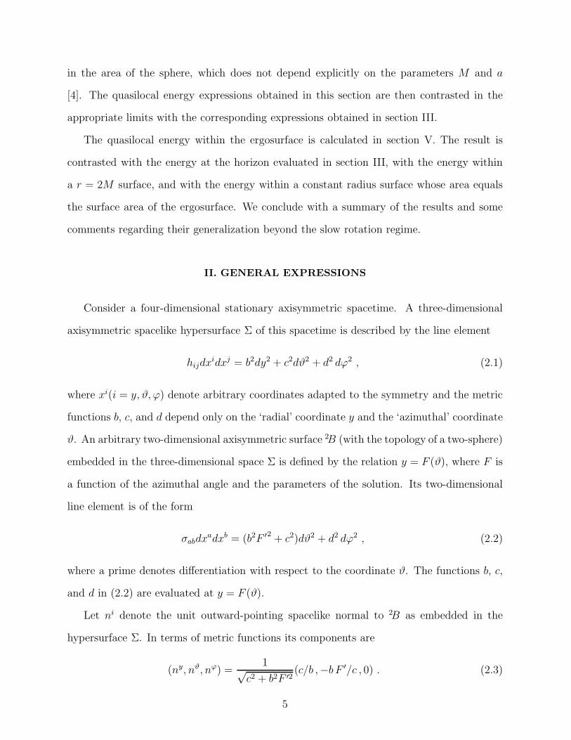
in the area of the sphere, which does not depend explicitly on the parameters M and a
[4]. The quasilocal energy expressions obtained in this section are then contrasted in the
appropriate limits with the corresponding expressions obtained in section III.
The quasilocal energy within the ergosurface is calculated in section V. The result is
contrasted with the energy at the horizon evaluated in section III, with the energy within
a r = 2M surface, and with the energy within a constant radius surface whose area equals
the surface area of the ergosurface. We conclude with a summary of the results and some
comments regarding their generalization beyond the slow rotation regime.
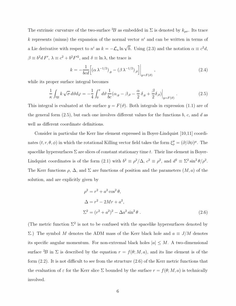
II. GENERAL EXPRESSIONS
Consider a four-dimensional stationary axisymmetric spacetime. A three-dimensional
axisymmetric spacelike hypersurface Σ of this spacetime is described by the line element
hijdxidxj = b2dy2 + c2dϑ2 + d2 dϕ2 , (2.1)
where xi(i = y, ϑ, ϕ) denote arbitrary coordinates adapted to the symmetry and the metric
functions b, c, and d depend only on the ‘radial’ coordinate y and the ‘azimuthal’ coordinate
ϑ. An arbitrary two-dimensional axisymmetric surface 2B (with the topology of a two-sphere)
embedded in the three-dimensional space Σ is defined by the relation y = F (ϑ), where F is
a function of the azimuthal angle and the parameters of the solution. Its two-dimensional
line element is of the form
σabdxadxb = (b2F ′2 + c2)dϑ2 + d2 dϕ2 , (2.2)
where a prime denotes differentiation with respect to the coordinate ϑ. The functions b, c,
and d in (2.2) are evaluated at y = F (ϑ).
Let ni denote the unit outward-pointing spacelike normal to 2B as embedded in the
hypersurface Σ. In terms of metric functions its components are
(ny, nϑ, nϕ) =1√
c2 + b2F ′2(c/b ,−b F ′/c , 0) . (2.3)
5
The extrinsic curvature of the two-surface 2B as embedded in Σ is denoted by kµν . Its trace
k represents (minus) the expansion of the normal vector ni and can be written in terms of
a Lie derivative with respect to ni as k = −Ln ln√
h. Using (2.3) and the notation α ≡ c2d,
β ≡ b2d F ′, λ ≡ c2 + b2F ′2, and δ ≡ ln λ, the trace is
k = − 1
bcd
[
(α λ−1/2),y − (β λ−1/2),ϑ
]
∣
∣
∣
∣
∣
y=F (ϑ)
, (2.4)
while its proper surface integral becomes
1
κ
∫
2Bk√
σ dϑdϕ = −1
4
∫ π
0dϑ
1
bc(α,y − β,ϑ −
α
2δ,y +
β
2δ,ϑ)
∣
∣
∣
∣
y=F (ϑ). (2.5)
This integral is evaluated at the surface y = F (ϑ). Both integrals in expression (1.1) are of
the general form (2.5), but each one involves different values for the functions b, c, and d as
well as different coordinate definitions.
Consider in particular the Kerr line element expressed in Boyer-Lindquist [10,11] coordi-
nates (t, r, θ, φ) in which the rotational Killing vector field takes the form ξµφ = (∂/∂φ)µ. The
spacelike hypersurfaces Σ are slices of constant stationary time t. Their line element in Boyer-
Lindquist coordinates is of the form (2.1) with b2 ≡ ρ2/∆, c2 ≡ ρ2, and d2 ≡ Σ2 sin2 θ/ρ2.
The Kerr functions ρ, ∆, and Σ are functions of position and the parameters (M, a) of the
solution, and are explicitly given by
ρ2 = r2 + a2 cos2 θ,
∆ = r2 − 2Mr + a2,
Σ2 = (r2 + a2)2 − ∆a2 sin2 θ . (2.6)
(The metric function Σ2 is not to be confused with the spacelike hypersurfaces denoted by
Σ.) The symbol M denotes the ADM mass of the Kerr black hole and a ≡ J/M denotes
its specific angular momentum. For non-extremal black holes |a| ≤ M . A two-dimensional
surface 2B in Σ is described by the equation r = f(θ; M, a), and its line element is of the
form (2.2). It is not difficult to see from the structure (2.6) of the Kerr metric functions that
the evaluation of ε for the Kerr slice Σ bounded by the surface r = f(θ; M, a) is technically
involved.
6
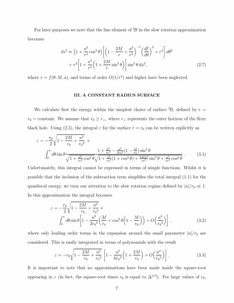
For later purposes we note that the line element of 2B in the slow rotation approximation
becomes
ds2 ≈(
1 +a2
r2cos2 θ
)
[
(
1 − 2M
r+
a2
r2
)−1(df
dθ
)2
+ r2
]
dθ2
+ r2
[
1 +a2
r2
(
1 +2M
rsin2 θ
)
]
sin2 θ dφ2, (2.7)
where r = f(θ; M, a), and terms of order O(1/r4) and higher have been neglected.
III. A CONSTANT RADIUS SURFACE
We calculate first the energy within the simplest choice of surface 2B, defined by r =
r0 = constant. We assume that r0 ≥ r+, where r+ represents the outer horizon of the Kerr
black hole. Using (2.5), the integral ε for the surface r = r0 can be written explicitly as
ε = −r0
2
√
1 − 2M
r0+
a2
r02×
∫ π
0dθ sin θ
1 + a2
r02 − a2
2r02 (1 − M
r0
) sin2 θ√
1 + a2
r02 cos2 θ
√
1 + a2
r02 (1 + cos2 θ) + 2Ma2
r03 sin2 θ + a4
r04 cos2 θ
. (3.1)
Unfortunately, this integral cannot be expressed in terms of simple functions. Whilst it is
possible that the inclusion of the subtraction term simplifies the total integral (1.1) for the
quasilocal energy, we turn our attention to the slow rotation regime defined by |a|/r0 ≪ 1.
In this approximation the integral becomes
ε = −r0
2
√
1 − 2M
r0+
a2
r02×
∫ π
0dθ sin θ
[
1 − a2
2r02
(
M
r0+ cos2 θ
(
1 − M
r0
))
+ O(
a4
r04
)
]
, (3.2)
where only leading order terms in the expansion around the small parameter |a|/r0 are
considered. This is easily integrated in terms of polynomials with the result
ε = −r0
√
1 − 2M
r0+
a2
r02
[
1 − a2
6r02
(
1 +2M
r0
)
+ O(
a4
r04
)
]
. (3.3)
It is important to note that no approximations have been made inside the square-root
appearing in ε (in fact, the square-root times r0 is equal to ∆1/2). For large values of r0,
7
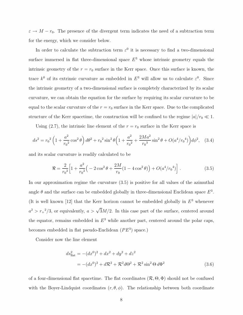
ε → M − r0. The presence of the divergent term indicates the need of a subtraction term
for the energy, which we consider below.
In order to calculate the subtraction term ε0 it is necessary to find a two-dimensional
surface immersed in flat three-dimensional space E3 whose intrinsic geometry equals the
intrinsic geometry of the r = r0 surface in the Kerr space. Once this surface is known, the
trace k0 of its extrinsic curvature as embedded in E3 will allow us to calculate ε0. Since
the intrinsic geometry of a two-dimensional surface is completely characterized by its scalar
curvature, we can obtain the equation for the surface by requiring its scalar curvature to be
equal to the scalar curvature of the r = r0 surface in the Kerr space. Due to the complicated
structure of the Kerr spacetime, the construction will be confined to the regime |a|/r0 ≪ 1.
Using (2.7), the intrinsic line element of the r = r0 surface in the Kerr space is
ds2 = r02(
1 +a2
r02
cos2 θ)
dθ2 + r02 sin2 θ
(
1 +a2
r02
+2Ma2
r03
sin2 θ + O(a4/r04))
dφ2, (3.4)
and its scalar curvature is readily calculated to be
ℜ =2
r02
[
1 +a2
r02
(
− 2 cos2 θ +2M
r0
(1 − 4 cos2 θ))
+ O(a4/r04)]
. (3.5)
In our approximation regime the curvature (3.5) is positive for all values of the azimuthal
angle θ and the surface can be embedded globally in three-dimensional Euclidean space E3.
(It is well known [12] that the Kerr horizon cannot be embedded globally in E3 whenever
a2 > r+2/3, or equivalently, a >
√3M/2. In this case part of the surface, centered around
the equator, remains embedded in E3 while another part, centered around the polar caps,
becomes embedded in flat pseudo-Euclidean (PE3) space.)
Consider now the line element
ds2flat = −(dx0)2 + dx2 + dy2 + dz2
= −(dx0)2 + dR2 + R2dΘ2 + R2 sin2 Θ dΦ2 (3.6)
of a four-dimensional flat spacetime. The flat coordinates (R, Θ, Φ) should not be confused
with the Boyer-Lindquist coordinates (r, θ, φ). The relationship between both coordinate
8
systems is important in the construction of the desired two-dimensional surfaces embedded
in flat space and deserves to be discussed. The line element (3.6) can be written in terms of
Boyer-Lindquist coordinates by defining
x0 =∫
du + dr
x = (r cos φ̃ + a sin φ̃) sin θ
y = (r sin φ̃ − a cos φ̃) sin θ
z = r cos θ , (3.7)
where the Kerr-Schild [10,11] coordinates (u, φ̃) are given by du = dt− (r2 + a2)/∆ dr, and
dφ̃ = dφ − a/∆ dr. (In fact, in terms of these coordinates the Kerr line element can be
written as the direct sum of two line elements, one of them being the flat element (3.6) ).
The relationship between (R, Θ, Φ) and (r, θ, φ) can be obtained easily by noting that the
coordinates (x, y, z) satisfy [10]
x2 + y2
r2 + a2+
z2
r2= 1 , (3.8)
and x2 + y2 + z2 = R2. In particular, one obtains R2 = r2 + a2 sin2 θ and
cos2 θ =r2 + a2
r2 + a2 cos2 Θcos2 Θ , sin2 θ =
r2
r2 + a2 cos2 Θsin2 Θ , (3.9)
which in the approximation |a| ≪ r reduce to
cos2 θ ≈ (1 + a2/r2 sin2 Θ) cos2 Θ
sin2 θ ≈ (1 − a2/r2 cos2 Θ) sin2 Θ . (3.10)
A flat three-dimensional slice of the flat spacetime (3.6) has line element
ds2 = dR2 + R2dΘ2 + R2 sin2 Θ dΦ2 . (3.11)
The equation for the desired two-dimensional surface in the flat slice is denoted by R = g(Θ),
where g is a function of the azimuthal angle Θ and the parameters (M, a, r0) of the surface
9
in Σ. Its intrinsic metric is obtained from (3.11). By virtue of (3.10), it is enough in the
slow rotation approximation to assume
g(Θ) = r0
(
1 +a2
r02ω(Θ) + O(a4/r0
4))
, (3.12)
where ω(Θ), a function of order one, is to be determined. The scalar curvature of this surface
is
ℜ0 =2
r02
[
1 − a2
r02
(
ω′′ + ω′ cot Θ + 2ω)
+ O(a4/r04)]
, (3.13)
where a prime denotes differentiation with respect to Θ. By equating the scalar curvatures
(3.5) and (3.13) and using (3.10) we obtain a differential equation for ω(Θ), whose solution
is ω(Θ) = −M/r0 cos 2Θ + 1/2 sin2 Θ. This implies that the radius of the surface in E3, as
a function of the azimuthal angle is given by
R = g(Θ) = r0
[
1 +a2
r02
(
1
2sin2 Θ − M
r0cos 2Θ
)
+ O(a4/r04)
]
. (3.14)
This equation describes a surface in flat Euclidean space E3 whose intrinsic curvature equals
the intrinsic curvature of a r = r0 surface in the Kerr slice. This surface, as embedded in E3,
is plotted in Figure 1 for particular values of M and a that satisfy the condition a2 ≪ r02. It
is a distorted sphere with its major axis along the equator. For fixed a2, the surface becomes
more oblate as M increases. Its intrinsic metric is given by
ds2 ≈ r02[
1 +a2
r02
(
sin2 Θ − 2M
r0
cos 2Θ)
]
(dΘ2 + sin2 Θ dΦ2) , (3.15)
whereas its area is
A = 4πr02
[
1 +2a2
3r02
(
1 +M
r0
)
+ O(a4/r04)
]
. (3.16)
The extrinsic curvature k0 of the surface (3.14) as embedded in the flat space (3.11), and
its proper integral can be calculated now using the expressions (2.4) and (2.5) adapted to
the coordinates (R, Θ, Φ). A long but direct computation gives the desired integral
ε0 =1
κ
∫
2Bk0√
σ dΘdΦ = −r0
[
1 +a2
3r02
(
1 +M
r0
)
+ O(a4/r04)
]
. (3.17)
10
The energy is obtained by subtracting (3.17) from (3.3), with the result
E = r0
[
1 −√
1 − 2M
r0+
a2
r02
]
+a2
6r0
[
2 +2M
r0+(
1 +2M
r0
)
√
1 − 2M
r0+
a2
r02
]
+r0 O(a4/r04) , (3.18)
where terms of order r0 O(a4/r04) and higher are considered negligible. Expression (3.18) is
the quasilocal gravitational energy of a (slowly rotating) Kerr slice Σ spatially bounded by
a surface of constant Boyer-Lindquist radial coordinate r0. We stress that no restrictions on
the mass M have been imposed in the calculation of the energy expression (3.18).
Several features of the above expression are noteworthy. In the asymptotic limit r0 → ∞,
the energy approaches the ADM energy M . In the limit of zero angular momentum the
quasilocal energy reduces to
E = r0 − r0
√
1 − 2M
r0, (3.19)
which, as expected, is the quasilocal energy (within a surface of radius r = r0) for a
Schwarzschild black hole of ADM mass M . The small mass limit (or equivalently, the
large radius limit) of the energy (3.18) is obtained by assuming M ≪ r0 in (3.18). In this
case
E = M +M2
2r0+
M3
2r02
+5M4
8r03− 7M2a2
6r03
+ r0 O(a4/r04) , (3.20)
where terms of order O(M4/r04) and O(M2a2/r0
4) have been preserved while terms of
order O(a4/r04) and higher have been neglected. The first term in (3.20) represents the
total energy at spatial infinity while the second term represents (minus) the Newtonian
gravitational potential energy associated with building a shell of radius r0 and mass M by
bringing the individual constituent particles from spatial infinity. As discussed in Ref. [1]
for the static case, the energy E in this approximation has the natural interpretation of the
total energy associated with assembling the gravitational system starting from the boundary
of radius r0, and it reflects indeed the energy within this boundary. Notice that no terms of
order r0 O(a2/r02) are present in (3.20).
11
It is of interest to invert the energy equation (3.18) to obtain the ADM mass M as a
function of the energy E, the size r0 of the cavity, and the specific angular momentum a.
This not only illustrates the interpretation of the different terms in the energy expression
but also, as mentioned in the introductory paragraphs, has relevance in the study of black
hole stable configurations in a gravitational microcanonical ensemble. In the limit of small
energy, the desired equation is
M = E(
1 − E
2r0
)
+ O(a2E2/r03) . (3.21)
In the limit a → 0 this expression is exact for all values of E and reduces to the expression
for the Schwarzschild ADM mass in terms of boundary radius and energy [3].
Expression (3.18) can be used to calculate the energy at the horizon whenever |a| ≪ r+
(or equivalently, whenever |a| ≪ M). The two-dimensional outer horizon [11] of a Kerr
black hole is a topological (but not a round) sphere of constant coordinate radius r0 = r+ =
M +(M2 −a2)1/2. In the present approximation, r+ = 2M(1−a2/4M2 +O(a4/M4)). Since
ε(r+) = 0, the energy becomes
E(r0 = r+) = r+
[
1 +a2
2r+2
+ O(a4/r+4)]
= 2M[
1 − a2
8M2+ O(a4/r+
4)]
. (3.22)
Recall now that the irreducible mass Mi of a Kerr black hole [13] is proportional to the
square root of the surface area of the horizon and can be written as
Mi =1
2
(
r+2 + a2
)1/2=
r+
2
[
1 +a2
2r+2
+ O(a4/r+4)]
. (3.23)
Therefore the quasilocal energy (3.22) at the horizon equals twice the irreducible mass,
E(r0 = r+) = 2Mi[1 + O(a4/Mi4)] (3.24)
to leading order in the slow rotation regime. This is a very attractive property of the energy
(3.18), valid perhaps beyond the present approximations, and constitutes one of the main
results of this paper.
12
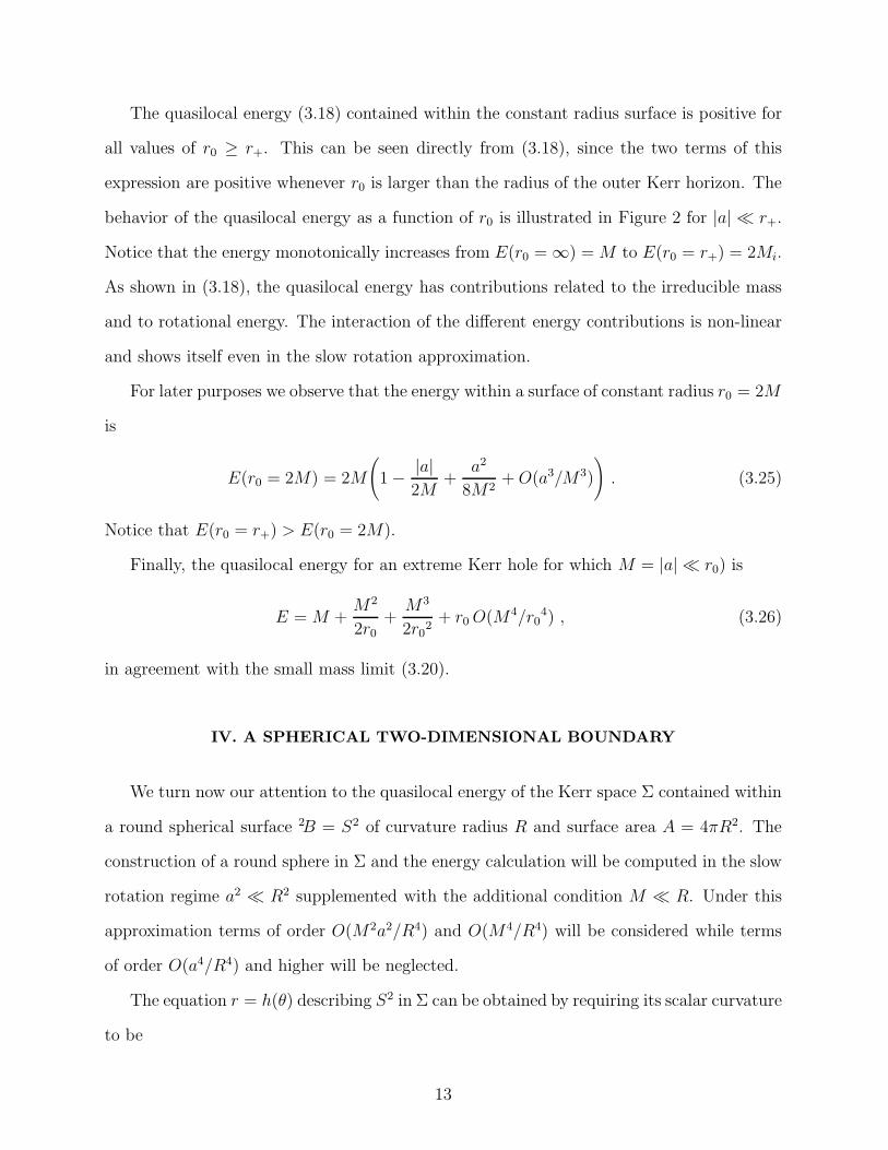
The quasilocal energy (3.18) contained within the constant radius surface is positive for
all values of r0 ≥ r+. This can be seen directly from (3.18), since the two terms of this
expression are positive whenever r0 is larger than the radius of the outer Kerr horizon. The
behavior of the quasilocal energy as a function of r0 is illustrated in Figure 2 for |a| ≪ r+.
Notice that the energy monotonically increases from E(r0 = ∞) = M to E(r0 = r+) = 2Mi.
As shown in (3.18), the quasilocal energy has contributions related to the irreducible mass
and to rotational energy. The interaction of the different energy contributions is non-linear
and shows itself even in the slow rotation approximation.
For later purposes we observe that the energy within a surface of constant radius r0 = 2M
is
E(r0 = 2M) = 2M
(
1 − |a|2M
+a2
8M2+ O(a3/M3)
)
. (3.25)
Notice that E(r0 = r+) > E(r0 = 2M).
Finally, the quasilocal energy for an extreme Kerr hole for which M = |a| ≪ r0) is
E = M +M2
2r0+
M3
2r02
+ r0 O(M4/r04) , (3.26)
in agreement with the small mass limit (3.20).
IV. A SPHERICAL TWO-DIMENSIONAL BOUNDARY
We turn now our attention to the quasilocal energy of the Kerr space Σ contained within
a round spherical surface 2B = S2 of curvature radius R and surface area A = 4πR2. The
construction of a round sphere in Σ and the energy calculation will be computed in the slow
rotation regime a2 ≪ R2 supplemented with the additional condition M ≪ R. Under this
approximation terms of order O(M2a2/R4) and O(M4/R4) will be considered while terms
of order O(a4/R4) and higher will be neglected.
The equation r = h(θ) describing S2 in Σ can be obtained by requiring its scalar curvature
to be
13
ℜ =2
R2, (4.1)
where R is a positive constant. The function h depends on the azimuthal angle and the
parameters (M, a, R), and in the slow rotation approximation takes the form
h(θ) = R(
1 +a2
R2η(θ) + O(a4/R4)
)
, (4.2)
where η(θ) is a function of order one. Substitution of (4.2) in (2.7) gives us a surface line
element whose intrinsic curvature is
ℜ =2
R2
[
1 − a2
R2
(
η′′ + η′ cot θ + 2η + 2 cos2 θ +2M
R(4 cos2 θ − 1)
)
+ O(a4/R4)]
, (4.3)
where a prime in this section denotes differentiation with respect to the Boyer-Lindquist
coordinate θ. By equating the scalar curvatures (4.3) with the scalar curvature (4.1) of a
round sphere one obtains a differential equation for η(θ), whose solution is η(θ) = MR
cos 2θ−12sin2 θ. Therefore, a two-dimensional round sphere S2 of curvature radius R in a slowly
rotating Kerr space Σ is described by the equation
r = h(θ) = R[
1 − a2
2R2sin2 θ +
a2M
R3cos 2θ + O(a4/R4)
]
. (4.4)
As expected from the behavior of the Boyer-Lindquist coordinates, the coordinate radius
of the sphere S2 is larger at the poles than at the equator. Its line element in the current
approximation is
ds2 = R2
[
1 +a2
R2
(
1 +2M
R
)
cos 2θ + O(a4/R4)
]
dθ2
+ R2 sin2 θ
[
1 +a2
R2
(
1 +2M
R
)
cos2 θ + O(a4/R4)
]
dφ2 . (4.5)
It can easily be verified that the area of this surface is A = 4πR2.
The quasilocal energy integral ε can now be calculated directly from the general expres-
sion (2.5) with b2 = ρ2/∆, c2 = ρ2, and d2 = Σ2 sin2 θ/ρ2, and by replacing the coordinates
(y, ϑ, ϕ) by (r, θ, φ). The Kerr metric functions ρ2, ∆, and Σ2, evaluated at the spherical
surface (4.4), are
14
ρ2(θ) = R2
[
1 +a2
R2(2 cos2 θ − 1) +
2a2M
R3(2 cos2 θ − 1) + O(a4/R4)
]
,
∆(θ) = R2
[
1 − 2M
R+
a2
R2cos2 θ +
a2M
R3(3 cos2 θ − 1) +
2a2M2
R4(1 − 2 cos2 θ) + O(a4/R4)
]
,
Σ2(θ) = R4
[
1 +a2
R2(3 cos2 θ − 1) +
2a2M
R3(3 cos2 θ − 1) + O(a4/R4)
]
, (4.6)
in the present approximation. The integrand becomes a function of (M, a, R) and the coor-
dinate θ. A long but direct calculation gives the total integral
ε = −R(
1 − 2M
R
)1/2[
1 +M2a2
R4
(
1 − 2M
R
)
−1
+ O(a4/R4)
]
. (4.7)
As expected, this expression is divergent for large R. The subtraction term is easily calcu-
lated in the present case since a two-dimensional sphere can always be embedded in E3. A
straightforward calculation gives k0 = −2/R and
ε0 = −R . (4.8)
By subtracting (4.8) from (4.7) one obtains the total energy, which can be written in our
approximation as
E = M +M2
2R+
M3
2R2+
5M4
8R3− M2a2
R3+ R O(a4/R4) . (4.9)
This expression gives the quasilocal gravitational energy of a Kerr space Σ (with specific
angular momentum a2 ≪ R2 and mass M ≪ R) spatially bounded by a round sphere of
surface area A = 4πR2. Observe that the specific angular momentum a shows itself only at
fourth order in E.
We discuss now some properties of the expression (4.9). The energy tends to M as R
tends to infinity and in the zero angular momentum limit one recovers the energy expression
(3.19) for a Schwarzschild black hole (this limit is expected since a two-surface of constant
radius r0 in the Schwarzschild spacetime is also a round sphere.) Observe from expression
(4.7) that a round spherical surface of area A = 4πR2 surrounding a (slowly) rotating Kerr
black hole of mass M ≪ R contains less energy than a round spherical surface of the same
15
area surrounding a Schwarzschild black hole of mass M . Figure 3 illustrates the behavior of
the energy (4.9) as a function of the quantity R whenever M ≪ R.
It is interesting to contrast the values of quasilocal energy of Σ within different surfaces.
Comparing (4.9) with (3.20), we observe that the energy contained within a round sphere of
curvature radius R = l0 is larger than the energy contained within a topologically spherical
surface of Boyer-Lindquist radius r0 = l0 whenever l0 is large (that is, |a| ≪ l0, M ≪ l0).
We can compare also the energy associated with a round sphere of area A = 4πR2 with
the energy associated with a constant radius boundary of the same surface area. Under our
approximation the two areas coincide if
R ≈ r0
(
1 +a2
3r02
(
1 +M
r0
)
)
. (4.10)
As can be seen by substituting this in (4.9) and comparing the resulting energy with (3.20),
the energy within the sphere equals the energy within the constant radius surface in the
present approximation whenever R and r0 are large. This is not surprising since the relative
distortion between the constant radius surface and the sphere is very small for large radii.
V. ERGOSURFACE
The timelike limit surface (or ergosurface) of a Kerr black hole is the boundary of the
region in which particles travelling on a timelike curve can remain on an orbit of the Killing
vector field ξµt = (∂/∂t)µ (and so remain at rest with respect to spatial infinity) [11]. The
ergosurface is a topologically spherical surface described by r = r∗ ≡ M +(M2−a2 cos2 θ)1/2;
r∗ coincides with the outer horizon radius r+ at the poles and equals 2M at the equator.
Since the ergosurface is neither a constant radius surface nor a round sphere, expressions
(3.18) and (4.9) cannot be used to estimate the quasilocal energy within it. However, the
energy can be evaluated in the slow rotation approximation |a| ≪ M . The term ε can in
fact be evaluated directly from (2.5) for arbitrary values of angular momentum. The result
will not be presented here because, as for previous surfaces, the integral cannot be written
16
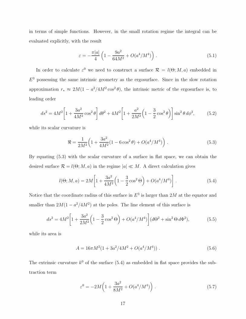
in terms of simple functions. However, in the small rotation regime the integral can be
evaluated explicitly, with the result
ε = −π|a|4
(
1 − 9a2
64M2+ O(a4/M4)
)
. (5.1)
In order to calculate ε0 we need to construct a surface R = l(Θ; M, a) embedded in
E3 possessing the same intrinsic geometry as the ergosurface. Since in the slow rotation
approximation r∗ ≈ 2M(1 − a2/4M2 cos2 θ), the intrinsic metric of the ergosurface is, to
leading order
ds2 = 4M2
[
1 +3a2
4M2cos2 θ
]
dθ2 + 4M2
[
1 +a2
2M2
(
1 − 3
2cos2 θ
)
]
sin2 θ dφ2, (5.2)
while its scalar curvature is
ℜ =1
2M2
(
1 +3a2
4M2(1 − 6 cos2 θ) + O(a4/M4)
)
. (5.3)
By equating (5.3) with the scalar curvature of a surface in flat space, we can obtain the
desired surface R = l(Θ; M, a) in the regime |a| ≪ M . A direct calculation gives
l(Θ; M, a) = 2M
[
1 +3a2
4M2
(
1 − 3
2cos2 Θ
)
+ O(a4/M4)
]
. (5.4)
Notice that the coordinate radius of this surface in E3 is larger than 2M at the equator and
smaller than 2M(1 − a2/4M2) at the poles. The line element of this surface is
ds2 = 4M2
[
1 +3a2
2M2
(
1 − 3
2cos2 Θ
)
+ O(a4/M4)
]
(dΘ2 + sin2 Θ dΦ2), (5.5)
while its area is
A = 16πM2(1 + 3a2/4M2 + O(a4/M4)) . (5.6)
The extrinsic curvature k0 of the surface (5.4) as embedded in flat space provides the sub-
traction term
ε0 = −2M(
1 +3a2
8M2+ O(a4/M4)
)
. (5.7)
17
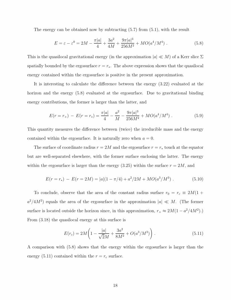
The energy can be obtained now by subtracting (5.7) from (5.1), with the result
E = ε − ε0 = 2M − π|a|4
+3a2
4M+
9π|a|3256M2
+ MO(a4/M4) . (5.8)
This is the quasilocal gravitational energy (in the approximation |a| ≪ M) of a Kerr slice Σ
spatially bounded by the ergosurface r = r∗. The above expression shows that the quasilocal
energy contained within the ergosurface is positive in the present approximation.
It is interesting to calculate the difference between the energy (3.22) evaluated at the
horizon and the energy (5.8) evaluated at the ergosurface. Due to gravitational binding
energy contributions, the former is larger than the latter, and
E(r = r+) − E(r = r∗) =π|a|4
− a2
M− 9π|a|3
256M2+ MO(a4/M4) . (5.9)
This quantity measures the difference between (twice) the irreducible mass and the energy
contained within the ergosurface. It is naturally zero when a = 0.
The surface of coordinate radius r = 2M and the ergosurface r = r∗ touch at the equator
but are well-separated elsewhere, with the former surface enclosing the latter. The energy
within the ergosurface is larger than the energy (3.25) within the surface r = 2M , and
E(r = r∗) − E(r = 2M) = |a|(1 − π/4) + a2/2M + MO(a3/M3) . (5.10)
To conclude, observe that the area of the constant radius surface r0 = rc ≡ 2M(1 +
a2/4M2) equals the area of the ergosurface in the approximation |a| ≪ M . (The former
surface is located outside the horizon since, in this approximation, r+ ≈ 2M(1− a2/4M2).)
From (3.18) the quasilocal energy at this surface is
E(rc) = 2M
(
1 − |a|√2M
+3a2
8M2+ O(a3/M3)
)
. (5.11)
A comparison with (5.8) shows that the energy within the ergosurface is larger than the
energy (5.11) contained within the r = rc surface.
18
VI. SUMMARY
We have calculated the quasilocal energy (1.1) for the constant stationary time slice of
the Kerr spacetime contained within three different classes of boundary surfaces, namely,
constant radius surfaces, round spheres, and the ergosurface. These surfaces were chosen
because they play a special role in the physics of Kerr black holes. The calculations were
confined to the slow rotation regime |a| ≪ r. Unless explicitly stated, the mass M was
not restricted by any approximation. Energy expressions in the small mass (large radius)
limit were also presented. For surfaces close to the outer horizon of the Kerr black hole,
the quasilocal energy was explicitly calculated under the assumption that |a| ≪ r+ (or
equivalently, |a| ≪ M). Under these approximations, the curvature of the surfaces involved
was positive everywhere and the embedding in E3 could be done explicitly. In particular, the
quasilocal energy within constant radius surfaces and spherical surfaces is a monotonically
decreasing function of the radius. The energy within the ergosurface is larger than M ,
and the energy at the horizon equals twice the irreducible mass of the black hole. These
results constitute a natural extension to stationary black holes of previously known results
concerning quasilocal energy for static black holes.
Short of an exact evaluation of (1.1), it is perhaps not unreasonable to look for a quasilocal
energy expression (say, for r = r0 surfaces) that satisfies the four conditions: (1) E → M
as r → ∞, (2) E → 2Mi as r → r+, (3) E → r0 − r0(1 − 2M/r0)1/2 as a → 0, and
(4) E → Eqn.(3.18) in the limit |a| ≪ r0. Whereas it is easy to find expressions that
fulfill conditions (1)-(3), it is difficult to satisfy (4). In particular, relations of the form
r0 − r0 (1 − r+/r0)1/2 or r0 − r0 (1 − 2Mi/r0)
1/2 do not satisfy the above criteria. In any
case, the desired expression for the quasilocal energy of the Kerr space Σ has to reflect the
peculiarities of the embedding of boundary surfaces in E3 in the fast rotation regime. We
hope to return to this issue elsewhere.
19
ACKNOWLEDGMENTS
It is a pleasure to thank Werner Israel for his encouragement and for his critical reading
of the manuscript. Research support was received from the Natural Science and Engineering
Research Council of Canada through a Canada International Fellowship.
20
REFERENCES
[1] J. D. Brown and J. W. York, Jr., Phys. Rev. D47, 1407 (1993).
[2] R. P. Kerr, Phys. Rev. Lett., 11, 237 (1963).
[3] J. W. York, Jr., Phys. Rev. D33, 2092 (1986); B. F. Whiting and J. W. York, Jr., Phys.
Rev. Lett., 61, 1336 (1988).
[4] J. D. Brown, E. A. Martinez, and J. W. York, Jr., Phys. Rev. Lett., 66, 2281 (1991);
in Nonlinear Problems in Relativity and Cosmology, edited by J. R. Buchler, S. L.
Detweiler, and J.R. Ipser (New York Academy of Sciences, New York, 1991).
[5] J. Katz, D. Lynden-Bell and W. Israel, Class. Quantum Grav. 5, 971 (1988).
[6] S. A. Hayward, Phys. Rev. D49, 831 (1994).
[7] G. W. Gibbons and S. W. Hawking, Phys. Rev. D15 , 2752 (1977).
[8] J. D. Brown and J. W. York, Jr., Phys. Rev. D47, 1420 (1993).
[9] R. Arnowitt, S. Deser, and C. W. Misner, in Gravitation: An Introduction to Current
Research, edited by L. Witten (Wiley, New York, 1962).
[10] R. H. Boyer and R. W. Lindquist, J. Math. Phys. 8, 265 (1967).
[11] C. W. Misner, K. S. Thorne and J. A. Wheeler, Gravitation, W. H. Freeman and Sons,
San Francisco, 1973.
[12] L. Smarr, Phys. Rev. D7, 289 (1973).
[13] D. Christodoulou and R. Ruffini, Phys. Rev. D4, 3552 (1971).
21
FIGURE CAPTIONS
Figure 1: Embedding diagram (in three-dimensional Euclidean space E3) of a two-
dimensional surface whose intrinsic geometry coincides with the intrinsic
geometry of a r = r0 surface in the Kerr space Σ. The figure corresponds
to particular values of M and a that satisfy the condition a2 ≪ r02. For
fixed a2, the surface becomes more oblate as M increases.
Figure 2: The quasilocal energy as a function of the coordinate radius r0 of 2B in
the case |a| ≪ r+.
Figure 3: The quasilocal energy as a function of the curvature radius R of a round
spherical surface for the case M = 1, |a| = .2. The energy approaches M
at spatial infinity.
22

This figure "fig1-1.png" is available in "png" format from:
http://arXiv.org/ps/gr-qc/9405033v2

This figure "fig1-2.png" is available in "png" format from:
http://arXiv.org/ps/gr-qc/9405033v2

This figure "fig1-3.png" is available in "png" format from:
http://arXiv.org/ps/gr-qc/9405033v2


