Photographic assessment of temperate forest understory phenology in relation to springtime meteorological drivers

ORIGINAL PAPER

Photographic assessment of temperate forestunderstory phenology in relation to springtimemeteorological drivers

Liang Liang & Mark D. Schwartz & Songlin Fei

Received: 2 April 2010 /Revised: 22 February 2011 /Accepted: 22 February 2011 /Published online: 10 May 2011# ISB 2011

Abstract Phenology shows sensitive responses to seasonalchanges in atmospheric conditions. Forest understoryphenology, in particular, is a crucial component of theforest ecosystem that interacts with meteorological factors,and ecosystem functions such as carbon exchange andnutrient cycling. Quantifying understory phenology ischallenging due to the multiplicity of species and hetero-geneous spatial distribution. The use of digital photographyfor assessing forest understory phenology was systemati-cally tested in this study within a temperate forest duringspring 2007. Five phenology metrics (phenometrics) wereextracted from digital photos using three band algebra andtwo greenness percentage (image binarization) methods.Phenometrics were compared with a comprehensive suite ofconcurrent meteorological variables. Results show thatgreenness percentage cover approaches were relativelyrobust in capturing forest understory green-up. Derivedspring phenology of understory plants responded toaccumulated air temperature as anticipated, and with day-to-day changes strongly affected by estimated moistureavailability. This study suggests that visible-light photo-

graphic assessment is useful for efficient forest understoryphenology monitoring and allows more comprehensive datacollection in support of ecosystem/land surface models.

Keywords Landscape phenology . Forest understory .

Temperate forest . Digital photography . EOS LandValidation Core Sites

Introduction

Phenology is the study of periodical plant and animal lifecycle events as influenced by environmental factors,especially weather and climate (Schwartz 2003). Weatherfluctuations and long-term climate change constantly affectthe timing behaviors of biological systems. Assessments ofglobal change impacts have identified phenology as a keyindicator of ecosystem alteration (IPCC 2007; Morisette etal. 2009). Temperate forests, in particular, are important forassessing changes of ecosystem properties given thetypically strong seasonality that is integral to annualtemperature regimes of mid-latitude land regions. Further,understory plants form an important component influencingthe general composition, nutrient cycling, and health offorests (Fei and Steiner 2008; Gilliam and Roberts 2003;Kaeser et al. 2008; Yarie 1980) and contribute to ecosystemcarbon and water exchange (Drewitt et al. 2002; Pfitsch andPearcy 1989). Phenology of understory plants is influencedby micro-environmental conditions different from that oftree canopies, and could potentially respond to climatechange in unique ways within forests (Beatty 1984; Kudoet al. 2008; Rich et al. 2008). In addition, high resolutionmeasurement of understory phenological progressionallows for a more comprehensive characterization of forestvegetation dynamics, and enhances the accuracy of

L. Liang (*)Department of Forestry, University of Kentucky,223 T.P. Cooper Bldg,Lexington, KY 40546–0073, USAe-mail: [email protected]

M. D. SchwartzDepartment of Geography, University of Wisconsin-Milwaukee,P.O. Box 413, Milwaukee, WI 53201–0413, USAe-mail: [email protected]

S. FeiDepartment of Forestry, University of Kentucky,204 T.P. Cooper Bldg,Lexington, KY 40546–0073, USAe-mail: [email protected]

Int J Biometeorol (2012) 56:343–355DOI 10.1007/s00484-011-0438-1

validation efforts for satellite-based vegetation indices(Liang and Schwartz 2009). Given all these importantaspects, more in-depth investigations are needed to furtherunderstanding of understory phenology in relation to forestecosystem changes. Also, being able to detect detailedpatterns of micrometeorological factors that influenceforest understory phenology is crucial for gaining insightconcerning how forest ecosystem structure might respondto global climate change.

Phenology of typical understory plants, such as grassand herb species, can be described in detail according totheir respective growth stages, given sufficient observationtime (Henebry 2003; Meier 1997). However, it is difficultto conduct quick repetitive observations with detaileddescriptive protocols under field conditions, due to themultiplicity of species intertwined within a small area,diverse morphologies of plants, distribution heterogeneityover the forest floor, and human resource constraints.Therefore, assessment using digital cameras could providea convenient approach to quickly capturing the green-upsequence of understory plants. In recent years, the use ofnetworked digital cameras has been employed for regularlyrecording phenological changes of forest canopies (Ahrendset al. 2009; Richardson et al. 2009). Automated camerasystems have also been used to record phenology ofselected understory species of interest in managed environ-ments (Crimmins and Crimmins 2008; Graham et al. 2009).To our knowledge, systematic sampling of natural forestunderstory phenology has only rarely been conducted,partly due to a lack of efficient approaches that wouldallow observers to conduct recurrent measurement andanalysis for high resolution samples with desired accuracy,given the challenges mentioned above. In this study, wesystematically recorded high resolution understory phenol-ogy using frequent digital photography, and tested differentmethods for deriving phenological metrics (phenometrics)from digital photos. Using selected phenometrics, we furtherexamined springtime understory phenology in the context ofits meteorological drivers through a focused spatiotemporalanalysis.

Materials and methods

Study site description

The field work was conducted in the ChequamegonNational Forest, near Park Falls, Wisconsin. The study siteis located in the vicinity of a television tower (WLEF,45.946°N, 90.272°W) which also supports AmeriFlux eddycovariance instruments, and is an Earth Observing System(EOS) Land Validation Core Site. The gentle slopingtopography underlying the forest is covered with soils

developed from parent materials of glacial-fluvial deposits(Martin 1965). The regional climate is humid continentalwith annual average temperature of 4.8°C, and annualprecipitation around 810 mm (Wisconsin Online: http://www.wisconline.com/counties/price/climate.html). Forestsin this limited study area are primarily composed of: (1)aspen/fir forest dominated by quaking aspen (Populustremuloides) and balsam fir (Abies balsamea), with otherspecies such as red maple (Acer rubrum) and white birch(Betula papyrifera); and (2) forested wetlands occupiedmainly by white cedar (Thuja occidentalis), balsam fir, andspeckled alder (Alnus regosa) (Ewers et al. 2002).

More than 100 understory species were identified in theforest under study (Brosofske et al. 2001). The compositionof understory cover ranges from grass, sedge and herba-ceous species in drier habitats, to sphagnum moss inmoister habitats, often mixed with seedlings and saplingsof woody species. Primary understory plants observedinclude species such as Canada mayflower (Maianthemumcanadense), bunchberry dogwood (Cornus canadensis),dewberry (Rubus spp.), starflower (Trientalis borealis),barren strawberry (Waldsteinia spp.), wild strawberry(Fragaria vesca), groundpine (Lycopodium dendroideum),Virginia creeper (Parthenocissus quinquefolia), goldenrod(Solidago spp.), violet (Viola spp.), bedstraw (Galium spp.),peat moss (Sphagnum spp.), blueberry (Vaccinium spp.),woodfern (Dryopteris spp.), ladyfern (Athyrium spp.), panicgrass (Panicum spp.), and a variety of sedges (Carex spp.).Seedlings and saplings found to mix with other understoryplants were mainly red maple, balsam fir, and quaking aspen.

Phenology data collection

Field observation of understory vegetation phenology withinthe forest was conducted in spring 2007. Ground samplingwas done within an approximately 625×275 m area (Fig. 1).Twenty-one 1×1 m plots were set on selected spots alongexisting transects outlined according to a cyclic samplingdesign (Burrows et al. 2002; Liang and Schwartz 2009).Sixteen of these plots followed an equally spaced systematicsampling scheme along four transects with 175-m samplingintervals. The remaining five plots were deployed randomlyat additional locations empirically identified as representa-tive ground cover types, to increase the representativeness oflandscape heterogeneity. Each understory plot was laid outusing a PVC pipe “square” and marked with stakes at fourcorners.

Digital photography was used to obtain phenologicalsignals that represent the aggregated reflectance of multi-species green-up. Given previously mentioned challengesin regards to collecting phenological information forindividual understory species, we treated the fixed-sizedunderstory plots as basic observation units. Field work was

344 Int J Biometeorol (2012) 56:343–355

http://www.wisconline.com/counties/price/climate.html

http://www.wisconline.com/counties/price/climate.html

conducted during the morning or before early afternoon(1300 hours) of every other day from April 29 to May 25,2007 (14 days in total). A consumer-grade 5MP KodakDX4530 visible-light digital camera was used. The camerahad firmware version 1.0 installed and supported automaticwhite balance. The camera mode was set to automatic withauto-exposure enabled. Nadir-pointing images were takenover every plot at 1.5 m above the ground. The observertook care to make the images consistent position-wiseunder varying field conditions, and to take all images fromthe same height and at zenith above the ground (a sampleimage is shown in Fig. 2).

Meteorological measurements

Micrometeorological data were collected with HOBO dataloggers (Onset Computer) deployed at 27 locations across

the study area (Fig. 1). These data loggers were set to taketemperature and humidity measurements of the ambient air(at standard 1.5 m shelter height) at 10-min readingintervals. Recorded data were stored in memory withineach logger for later retrieval. HOBO recording wasinitiated on April 5, 2007 prior to the field campaign andrecovered on the last day of observation (May 25, 2007). Inaddition to the high resolution meteorological measure-ments, daily precipitation data from the closest officialweather station at Park Falls (approximately 8 miles, c.13 km west of the study site) were acquired through theNational Climatic Data Center (NCDC: http://www.ncdc.noaa.gov/oa/ncdc.html). The time span of these data ranfrom January 1 to May 31, 2007. Precipitation data weremainly used to compare with air humidity measurementswhich supported high resolution analysis.

Phenometrics derivation

A visible-light digital camera allows assessments ofvegetation greening, despite the lack of a near infraredspectral band that is often indispensible for vegetationremote sensing (Jensen 2000; Lukina et al. 1999). Digitalimages taken with a visible-light camera natively containseparable red-green-blue (RGB) color bands. Band algebrasand percentage cover estimates (image binarization) canhence be used to derive signals of plant greenness, and inturn to characterize plant phenology (Ahrends et al. 2008;Graham et al. 2006; Lukina et al. 1999; Richardson et al.2007). Besides using native RGB bands, a recent studysuggested an alternative approach based on hue-saturation-luminance (HSL) color space, which may provide moreaccurate estimation of plant color change by separatingluminance/brightness (potentially affected by illuminationconditions) from the hue (Graham et al. 2009).

The HSL color space is represented with a cylindermodel. The angle around the central axis of the cylinder

Fig. 2 A sample digital photo of an understory plot taken on May 25,2007; cropped to contain the 1×1 m plot area (original photo is incolor, presented here in gray scale)

Fig. 1 Locations of understoryplots and HOBO loggers over-laid on a QuickBird image-derived Normalized DifferenceVegetation Index (NDVI) mapshowing vegetation coverconditions on May 18, 2007

Int J Biometeorol (2012) 56:343–355 345

http://www.ncdc.noaa.gov/oa/ncdc.html

http://www.ncdc.noaa.gov/oa/ncdc.html

corresponds to hue, which represents the color or wavelengthof the pixel; the distance towards the axis corresponds tosaturation which represents the purity of color, and theheight of the cylinder corresponds to lightness (also referredto as intensity) which is the overall brightness of the scene asvarying from black to white. The HSL color spacerepresentation can be translated from RGB color bands(Conrac Corporation 1980; ERDAS 2008; Pratt 2001) usingthe following equations:

r ¼ M � R

M � m; g ¼ M � G

M � m; b ¼ M � B

M � mð1Þ

where R, G, B are each in the range of 0–1 (converted fromdigital numbers); r, g, b are each in the range of 0–1 (at leastone of r, g, or b values is 0, and at least one of the r, g, or bvalues is 1); M is the maximum value of R, G, or B, m is theminimum value of R, G, or B. Then, the lightness (L) in therange of 0–1 is computed as:

L ¼ M þ m

2ð2Þ

The saturation (S) in the range of 0–1 is calculated as:

S ¼ 0; IfM ¼ m ð3Þ

S ¼ M � m

M þ m; If L � 0:5 ð4Þ

S ¼ M � m

2�M � m; If L > 0:5 ð5Þ

Finally the hue (H) in the range of 0–360 is calculatedas:

H ¼ 0; If M ¼ m ð6Þ

H ¼ 60 2þ b� gð Þ; If R ¼ M ð7Þ

H ¼ 60 4þ r � bð Þ; If G ¼ M ð8Þ

H ¼ 60 6þ g � rð Þ; If B ¼ M ð9Þ

Preprocessing of digital images was conducted with thePaint.NET program. ERDAS Imagine 9.2 (ERDAS 2008)was used to perform band algebra, color space transforma-tion, and image analysis.

Each digital image was cropped to include only a 1 m2 plotarea marked out by four corner sticks. Three selectedmethods of combining RGB bands for phenology signalextraction were tested: (1) G/R (Graham et al. 2006); (2) 2G-

R-B (Richardson et al. 2007; Woebbecke et al. 1995); and(3) (G-R) / (G+R) (Brügger et al. 2007). Mean values of theband algebra estimates were calculated for all pixels withineach plot area. Percentage of green pixels was estimatedaccording to the concept of image binarization which haswide applications in the field of pattern recognition and hasbeen introduced into agricultural practices (Tellaeche et al.2008; Tian and Slaughter 1998). In this study, simplethreshold-based approaches were used to separate greencover from the background. For RGB bands, a criteria:G > R and G > B was applied to discriminate green pixelsfrom the background. The HSL-based approach firstconverted RGB to HSL color space; then thresholds (above192 and below 288) for green color within the hue valuerange (0–360) were applied. The results from both RGB-and HSL-based methods were binary images with greenpixels distinguished from the background. Areal percentagesof green pixels were then computed for all binary images.

Evaluating phenometrics

Inter-comparison of the resultant time series of fivephenometrics was made in regards to their differenttemporal variability. Standardization to a 0–1 ratio wasapplied to averaged time series using the algorithm:(phenometric value – phenometric minimum) / (phenomet-ric maximum – phenometric minimum). In addition todirect comparison, bi-daily increments of phenometricvalues were computed and compared to one anotheraccordingly. Coefficients of variation (CV) were computedfor bi-daily changes of phenometrics. We evaluated thestability which in this context indicates the performance ofa phenometric in regards to capturing a realistic phenolog-ical trend. In particular, this trend refers to the green-upprocess which normally advances without backward devel-opment during springtime, unless affected by disturbancessuch as insect outbursts or grazing, or by excessivedeprivation of required resources. Our basic assumptionsuggests that a stable phenometric representation shouldreflect a steady increase in greenness during the earlyspring under disturbance-free conditions. Throughout theobservation time period, no disturbances from wildlife werenoticed and all plots remained intact. Given these consid-erations, we expected the phenometrics derived to matchthe consistently upturning spring green-up process. Conse-quently, downward departures from a previous greennesslevel as indicated by negative bi-daily changes wouldsuggest measurement instability. We therefore used thiscriterion to infer the relative robustness of the fivephenometrics derived against potential errors and measure-ment uncertainties. More stable phenometrics were selectedin support of subsequent analysis regarding meteorologicaldrivers.


Processing meteorological variables

High frequency/intensity temperature and humidity meas-urements allowed detailed characterization of microme-teorological conditions. We first computed temperature andhumidity indices (daily maximum, mean, and minimum)averaged over the entire study area. These indices werecompared with precipitation data recorded at the nearbyofficial weather station. Pearson correlation coefficientswere calculated for precipitation and air humidity indices,including both absolute humidity and relative humidity. Forhigh resolution analysis, field-measured temperature, abso-lute humidity, and relative humidity data were interpolatedto understory plot locations using ordinary Kriging. Dailytemperature and humidity indices (maximum, mean, andminimum) for each plot were then computed. Accumulatedgrowing degree hours (AGDH) were calculated from hourlymean temperature based on a −0.6°C threshold (Schwartz1997) starting from April 5, 2007. It was assumed thatchilling requirement necessary for dormancy release(Schwartz 1997; Simpson 1990) was fulfilled prior to thisdate. In order to perform a more comprehensive examina-tion of potential meteorological drivers, air water potentialand vapor pressure deficit were calculated from temperatureand relative humidity (Buck 1981; Kirkham 2004; Lamberset al. 1998), and included in the analysis. Accumulatedhumidity indices were derived from hourly means ofmeasurements in like manner as AGDH. Given thatunderstory observations were taken bi-daily, “cross-daychange” (a prior day measure subtracts the value from theday before) of all meteorological variables was calculated.Lastly, antecedent 2-day accumulations of temperature andhumidity were computed in order to provide a short-termanalysis of accumulated meteorological conditions. A list ofthe meteorological variables used in the study is providedin Table 1. Climate data interpolation, processing andanalysis were performed using R (R Development CoreTeam 2009).

Examining meteorological drivers

Understory phenology was compared with both long-termand short-term meteorological conditions as described by acomprehensive suite of variables (see Table 1 for details).In addition to cumulative phenology, changes of pheno-metric values between two consecutive bi-daily observa-tions were calculated for each plot to correspond with day-to-day weather fluctuations. Meteorological drivers ofunderstory phenology were examined using linear multipleregression analysis. At the plot level, our field datarepresented a panel data structure with multi-date observa-tions from a group of fixed targets, with both temporal andspatial dimensions. In order to accommodate such a data

structure, linear multiple regression models were fitted todata using a panel linear model (plm) package in R(Croissant and Millo 2008). Phenometrics at each plot wereself-standardized by dividing an original value by the site-specific range (i.e., site maximum minus site minimum) toreduce site variability related to species compositiondiversity. Both standardized and raw datasets wereregressed against meteorological variables. For cumulativephenological time series, accumulated hourly means oftemperature, absolute humidity, relative humidity, waterpotential, and vapor pressure deficit were used as candidateexplanatory variables. Phenological changes between twoconsecutive observations were modeled with additionalvariables representing daily weather conditions, antecedentweather conditions, and cross-day weather changes.

Variable subset selection was first conducted for eachvariable group (such as temperature-based variables orabsolute humidity-based variables) using an exhaustivesearch approach supported by an R package: leaps (Miller2002). The leaps package returns variable subsets with datamulticollinearity minimized. Bayesian information criterion(BIC, provided in the leaps package in R) was used todetermine the best variable subsets with overfittingavoided. Variables chosen from different groups werecombined for a further-step selection via the same approachas described above. Final subsets of variables were thenused to fit linear panel data regression models. Alogarithmic transformation was applied to selected variablesbefore model building to correct heteroscedasticity in thedata. Hausman test (provided with the plm package in R)was performed to decide whether a fixed or random effectsub-model was appropriate. Finally, models with allcoefficients significant at the 99% confidence level wereretained. In addition to plot level analysis, phenometricsaveraged across plots over the entire study area werecompared with averaged meteorological variables usingordinary least squares linear models. Averaged variablesrepresented overall conditions of the entire landscape;therefore, they are also referred to as landscape-levelmeasures.

Results

Comparison of phenometrics

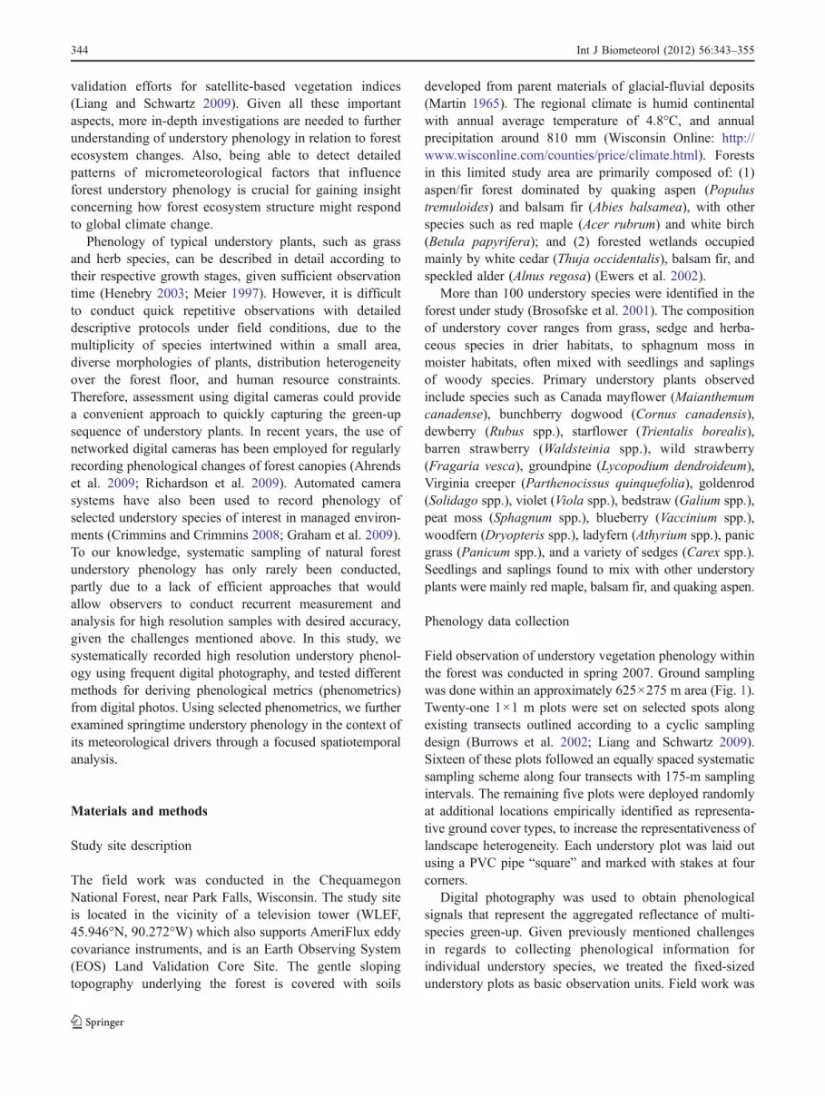
The five derived phenometrics demonstrated differingdegrees of variability over time (Fig. 3; Table 2). Standard-ization of phenometric time series to a range between 0 and1 allowed effective visual contrast in a unified scale frame,emphasizing their respective temporal response patterns.The among-metric differences were clearly seen in thevariability of their bi-daily changes (Fig. 4). Among the


band algebra-based phenometrics, bi-daily advance of banddifferencing (2G-R-B, excess green) and normalized differ-ence ratio ([G−R]/[G+R]) showed frequent negative changevalues over time. Coefficients of variation (CV) of thesetwo phenometrics were 268.03 and 178.85% respectively,greater than that of the other three phenometrics. Thesimple band ratio (G/R) time series demonstrated negativedepartures as well, yet at a smaller degree compared withthe last two metrics, with a CV value of 128.42%. Asdetailed previously, such phenomenon likely indicateinstability of these band algebra-based metrics againstpotential noise and measurement uncertainty, given thatobserved plant phenology consistently advanced during thestudy time period. Two greenness percentage measuresdemonstrated mostly positive increments over time withsmaller CV values (103.30 and 102.58%, respectively)compared to band algebra-based phenometrics. And, notice-ably, RGB-based and HSL-based greenness percentagemetrics resemble each other in regards to the phenologicalprogression and patterns of bi-daily change. Hence, the twogreenness percentage based phenometrics appeared to bemore robust against potential errors in capturing a realisticgreen-up process, and were adopted for subsequent evaluationof meteorological drivers.

Meteorological drivers of understory phenology

Humidity variables correlated with weather station precip-itation records significantly (Table 3). Correlation coeffi-cients with precipitation for both mean absolute humidityand relative humidity (r=0.44, and 0.61 ,respectively) weresignificant at the 95% confidence level. In particular,maximum absolute humidity (AHmax), and minimumrelative humidity (RHmin) showed highest correlations(r=0.68, and 0.68 ,respectively) with precipitation (signif-

icant at 99% confidence level). Further, humidity fluctua-tions appeared to correspond with the timing and magnitudeof precipitation occurrences on day-of-year (DOY) 128, 134–137, 139, 141, and 143–145 (Fig. 5). Given the significantcorrelations and temporal correspondence between precipi-tation and air humidity, field-measured humidity data wereused in characterizing the general moisture availability inrelation to understory growth in the below canopy environ-ment for high resolution analysis. Besides, peak temperatureswere found to occur often on the first days of rainy periods

Fig. 3 Spring time series of understory phenometrics averaged acrossplots; derived from five different photographic methods: 1) RGB-based greenness percentage; 2) (G-R)/(G+R); 3) 2G-R-B; 4) HSL-based greenness percentage; and 5) G/R ratio (all phenometric valueswere standardized)

Table 1 Summary of meteorological variables used in the analysis

Temperature(°C)

Absolutehumidity (g/m3)

Relativehumidity (%)

Air waterpotential (MPa)

Vapor pressuredeficit (kPa)

Daily mean Tmean AHmean RHmean WPmean VPDmean

Daily minimum Tmin AHmin RHmin WPmin VPDmin

Daily maximum Tmax AHmax RHmax WPmax VPDmax

Daily sum of hourly means GDH AHsum RHsum WPsum VPDsum

Accumulated hourly means AGDH AHcum RHcum WPcum VPDcum

"Cross-day change"(a prior day measure subtracts themeasure of the day before)

TmeanCg AHmeanCg RHmeanCg WPmeanCg VPDmeanCg

TminCg AHminCg RHminCg WPminCg VPDminCg

TmaxCg AHmaxCg RHmaxCg WPmaxCg VPDmaxCg

GDHCg AHsumCg RHsumCg WPsumCg VPDsumCg

Antecedent 2-day accumulation GDHPre2 AHsumPre2 RHsumPre2 WPsumPre2 VPDsumPre2

T Temperature, AH absolute humidity, RH relative humidity, WP water potential, VPD vapor pressure deficit, Cg “Cross-day Change” indicatesthe meteorological change occurred from the day before yesterday to yesterday in regards to an observation day


(such as DOY 134 and 143), followed by immediatetemperature declines. In addition, bi-daily increments ofphenometric values demonstrated temporal correspondenceswith increases of precipitation and humidity (Figs. 4 and 5).Especially for greenness percentage based phenometrics,accelerated increments were found on DOY 135 and 145which were preceded by DOY134 and 144 when consider-able amounts of precipitation occurred. An exception wasthat during the early part of spring season, a single

precipitation event on DOY 128 did not seem to match upwith any observed phenological advance.

For cumulative phenology, fitted panel linear modelsimplied that understory green-up responded to bothtemperature and humidity strongly. All models weresignificant at the 99% confidence level (Table 4). Resultsrevealed that accumulated growing degree hours (AGDH)alone could drive a model with a coefficient of determina-tion greater than 0.60. Yet humidity-based variables,accumulated vapor pressure deficit (VPDcum), or theaccumulated absolute humidity (AHcum), were also signif-icant explanatory variables. Models with humidity-basedvariables added significantly raised their explanatorypowers. RGB-based phenometrics were consistently betterpredicted with meteorological variables than HSL-basedphenometrics. Further, standardization appeared to raise theexplanatory power of models for RGB-based phenometricsin most cases, but only improved one case among modelsusing HSL-based phenometrics. Plotting the identifiedmeteorological drivers respectively against phenometrics,a linear dependency can be clearly seen in all cases (Fig. 6).

Panel linear models fitted for incremental phenologicalchange underperformed that of cumulative phenometrics atthe plot level. A few plot-level incremental phenologymodels were significant at confidence levels up to 99%.However, all model coefficients of determination werebelow 0.20. Therefore, analyzing meteorological drivers ofphenological change relied on landscape-level models,fitted with phenometrics and meteorological variablesaveraged across the entire study area. The landscape-levelvalues here simply indicate the averaged understoryphenometrics and meteorological conditions, with inter-plot variations smoothed. According to landscape-level

Fig. 4 Bi-daily changes of spring time series of understoryphenometrics averaged across plots as derived from the five differentphotographic methods; CV coefficient of variation

DOY RGB (%) (G−R)/(G+R) 2G-R-B (DN) HSL(%) G/R

Mean σ Mean σ Mean σ Mean σ Mean σ

119 9.98 5.72 −0.09 0.04 −5.31 7.62 6.91 4.17 0.87 0.05

121 9.44 3.73 −0.07 0.03 −8.42 8.50 6.75 2.83 0.89 0.04

123 9.26 4.90 −0.08 0.03 −6.90 9.14 6.22 3.44 0.88 0.05

125 10.20 6.84 −0.06 0.01 −13.62 11.67 7.58 4.15 0.90 0.02

127 12.60 7.53 −0.05 0.01 −11.35 12.36 9.58 4.57 0.91 0.02

129 13.32 6.71 −0.06 0.03 −1.92 13.99 9.50 5.01 0.90 0.04

131 16.61 7.87 −0.06 0.03 4.26 11.63 12.12 6.11 0.91 0.06

133 17.94 9.64 −0.05 0.02 −2.97 12.67 14.55 7.32 0.92 0.04

135 23.02 9.26 −0.06 0.02 −0.19 17.11 18.70 7.20 0.91 0.03

137 24.18 11.51 −0.06 0.04 12.35 15.88 18.38 9.13 0.92 0.07

139 24.02 9.67 −0.05 0.01 2.46 17.01 19.14 8.18 0.93 0.02

141 28.91 13.82 −0.04 0.03 14.10 22.90 23.70 11.88 0.95 0.06

143 33.39 15.48 −0.03 0.03 19.70 28.76 28.28 12.67 0.97 0.06

145 40.57 15.25 −0.02 0.03 32.32 26.39 33.98 12.53 1.00 0.07

Table 2 Averaged values ofphenometrics across plots withstandard deviation (σ)

DOY Day of year, DN digitalnumber


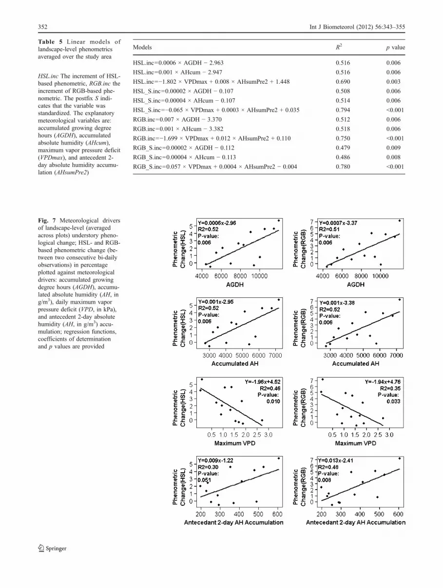
linear regression models, incremental phenology could beexplained by AGDH, AHcum, or a combination of dailymaximum vapor pressure deficit (VPDmax) and antecedent2-day absolute humidity accumulation (AHsumPre2), re-spectively (Table 5). All the models were significant at the99% confidence level. The first two models with eitherAGDH or AHcum as the predictor variable were similar intheir explanatory powers (R2=0.512-0.518). Models drivenby VPDmax and AHsumPre2 were considerably strongerwith coefficients of determination improvement rangingfrom 0.17 to 0.30 in comparison with models with long-term accumulated measures (AGDH, or AHcum) aspredictors. Investigated separately in scatter plots withlinear fit lines, phenological change was positively depen-dent on AGDH, AHcum, or AHsumPre2, and negativelydependent on VPDmax (Fig. 7). Humidity-based variablescould explain phenological change independently ofAGDH. This was unlike the relationship with cumulativephenometrics, which required AGDH in all models. Tosummarize, cumulative phenology was reasonably wellpredicted by thermal time (AGDH), but as far as the increment

of phenological progression is concerned, humidity-basedindices manifested themselves as independent explanatoryfactors. In addition, we found that standardized phenometricsonly out-performed non-standardized metrics for modelsdriven by VPDmax and AHsumPre2, but with reduced effectson the models driven by AGDH or AHcum. In the case oflandscape-level analysis, RGB- and HSL-based phenometricsdid not show marked differences overall as far as theexplanatory power of models is concerned, except that HSL-based models performed better than the RGB-based for thestandardized phenometrics.

Discussion

The greening of understory plants forms an importantaspect of temperate forest seasonal dynamics. As shown inthis study, digital photography is useful for more accuraterepeated measurement of understory phenology. Among thefive phenometrics derived from digital photos, greennesspercentage estimates were more robust against potentialerrors than band algebra-based metrics, although bandalgebra-based methods may be indispensible for character-izing vegetation change over fully covered plots. Thepotential errors that caused the instability of phenometricsmay stem mainly from illumination variability across plotsand uncertainties of the camera system. Different sitecanopy characteristics, sun angle/position, and cloudcondition at the time of observation unavoidably affectedthe reflectance from understory. The digital camera withauto-exposure enabled also increased the inconsistency ofphotos taken for different plots at different times, yet it mayhave balanced off the variability of light conditions to acertain degree. Nevertheless, the greenness percentageapproach appeared to be less sensitive to such uncertainties,and provided more realistic phenological progressionsignals.

Greenness percentage estimates from RGB and HSLcolor spaces responded to meteorological variables sensi-tively. The HSL-based phenometric was considered moreaccurate given its ability to reduce errors caused byillumination variability (Graham et al. 2009). In this study,according to regression model performance, RGB-basedphenometric appeared to be more responsive to micro-meteorological variations across plots than the HSL-based.

Fig. 5 Spring time series of daily meteorological measurements(PREC precipitation in mm, AHmax maximum absolute humidity ing/m3, RHmin minimum relative humidity in %, Tmean meantemperature in °C)

Table 3 Correlations between precipitation and air humidity variables

AHmax AHmin AHmean RHmax RHmin RHmean

PREC Pearson's r 0.68 0.35 0.44 0.31 0.68 0.61

p value <0.001 0.066 0.016 0.103 <0.001 <0.001

PREC Precipitation, AH absolute humidity, RH relative humidity


But among the landscape-level models created for averagedvariables, standardized HSL-based phenometric supportedbetter predictions. Given error sources discussed previously,as well as additional uncertainties from interpolation of

climate data, further assessment is still needed to bettercompare phenometrics estimated using the two-color models.

The assessment of meteorological variables revealeddetailed patterns of temperature and humidity in influencing

Table 4 Panel linear models of plot-level phenometrics

Phenometrics Explanatory variables and coefficients R2 p value

HSL AGDH (1.540) 0.650 <0.001

HSL AGDH (4.890), VPDcum (−4.444 ) 0.694 <0.001

HSL AGDH (−1.276), AHcum (3.018) 0.676 <0.001

HSL_S AGDH (1.539) 0.650 <0.001

HSL_S AGDH (4.890), VPDcum (−4.444) 0.694 <0.001

HSL_S AGDH (−1.616), AHcum (3.381) 0.695 <0.001

RGB AGDH (1.345) 0.715 <0.001

RGB AGDH (4.417 ), VPDcum (−4.073) 0.755 <0.001

RGB AGDH (−1.769), AHcum (3.337) 0.760 <0.001

RGB_S AGDH ( 1.344) 0.714 <0.001

RGB_S AGDH (4.654), VPDcum (−4.388 ) 0.770 <0.001

RGB_S AGDH (−1.887), AHcum (3.463) 0.774 <0.001

HSL-based phenometric (HSL) and RGB-based phenometric (RGB), both represented with greenness percentage cover. The postfix S indicatesthat the variable was standardized. The explanatory meteorological variables are: accumulated growing degree hours (AGDH), accumulated vaporpressure deficit (VPDcum), and accumulated absolute humidity (AHcum). All coefficients of explanatory variables were significant at the 99%confidence level (p values of respective coefficients are not presented here). A log transformation was applied to all variables to correctheteroscedasticity

Fig. 6 Meteorological driversof plot-level understory phenol-ogy: HSL- and RGB-basedphenometrics in percentageagainst identified meteorologicaldrivers: accumulated growingdegree hours (AGDH), accumu-lated vapor pressure deficit(VPD, in kPa), and accumulatedabsolute humidity (AH, in g/m3); regression model functions,coefficients of determinationand p values are provided.Heteroscedasticity shown in thedata was corrected in modelsusing a log transformation


Models R2 p value

HSL.inc=0.0006 × AGDH − 2.963 0.516 0.006

HSL.inc=0.001 × AHcum − 2.947 0.516 0.006

HSL.inc=−1.802 × VPDmax + 0.008 × AHsumPre2 + 1.448 0.690 0.003

HSL_S.inc=0.00002 × AGDH − 0.107 0.508 0.006

HSL_S.inc=0.00004 × AHcum − 0.107 0.514 0.006

HSL_S.inc=−0.065 × VPDmax + 0.0003 × AHsumPre2 + 0.035 0.794 <0.001

RGB.inc=0.007 × AGDH − 3.370 0.512 0.006

RGB.inc=0.001 × AHcum − 3.382 0.518 0.006

RGB.inc=−1.699 × VPDmax + 0.012 × AHsumPre2 + 0.110 0.750 <0.001

RGB_S.inc=0.00002 × AGDH − 0.112 0.479 0.009

RGB_S.inc=0.00004 × AHcum − 0.113 0.486 0.008

RGB_S.inc=0.057 × VPDmax + 0.0004 × AHsumPre2 − 0.004 0.780 <0.001

Table 5 Linear models oflandscape-level phenometricsaveraged over the study area

HSL.inc The increment of HSL-based phenometric, RGB.inc theincrement of RGB-based phe-nometric. The postfix S indi-cates that the variable wasstandardized. The explanatorymeteorological variables are:accumulated growing degreehours (AGDH), accumulatedabsolute humidity (AHcum),maximum vapor pressure deficit(VPDmax), and antecedent 2-day absolute humidity accumu-lation (AHsumPre2)

Fig. 7 Meteorological driversof landscape-level (averagedacross plots) understory pheno-logical change; HSL- and RGB-based phenometric change (be-tween two consecutive bi-dailyobservations) in percentageplotted against meteorologicaldrivers: accumulated growingdegree hours (AGDH), accumu-lated absolute humidity (AH, ing/m3), daily maximum vaporpressure deficit (VPD, in kPa),and antecedent 2-day absolutehumidity (AH, in g/m3) accu-mulation; regression functions,coefficients of determinationand p values are provided


understory plant phenology. Given the close relationshipfound between precipitation and air humidity, variablesderived from the latter were used to indirectly indicatemoisture availability. Variations of cumulative understoryphenology at plot level were affected by accumulatedmoisture in addition to accumulated heat. Incrementalphenology responded to heat and moisture accumulation, yethad stronger dependency on daily short-term change ofmoisture conditions. Such relationships first indicate agenerally accelerated rate of understory flushing withincreased spring warmth and water availability. Furthermore,they suggest that the occurrence of understory phenologicalchange was more directly triggered by precipitation events (asreflected by humidity increase at plot level) than risingtemperatures. Therefore, while accumulated heat and mois-ture provided a baseline for predicting spring growth ofunderstory plants, day-to-day moisture conditions determinedthe actual occurrence of phenological advance.

This detected phenomenon may be related to a relativelydry spring in the study area during the year of observation.From January to May 2007, total precipitation in the areawas 198 mm, which was 38 mm below the historicalaverage (1971–2000) of 236 mm during that 5-monthperiod of the year. The relatively dry weather mainlyoccurred in May (total 50 mm of precipitation) which fellfar short of the historical average of 80 mm. Hence, waterwas a limiting resource that hindered spring green-up ofunderstory plants during the time of observation. In amesic forest such as that investigated in this project,shallower root systems of understory species could be adirect cause of a stronger reliance on precipitation,especially during drought spells, in line with the typicalcases in semi-arid ecosystems (Brown and de Beurs 2008;Henebry 2003) and even tropical moist forests (Wright1991). This finding further demonstrates the usefulness ofphotographic assessment for capturing detailed understoryphenology information.

We identified the following limitations and drawbacks inrelation to meteorological driver assessment. First, due to alack of soil moisture data, air humidity was employed as aproxy for moisture availability. Although both absolutehumidity and relative humidity were found to be signifi-cantly correlated with precipitation, this measurement wasindirect and a large uncertainty may exist. This may beprovisionally workable under conditions where air humiditychange is closely connected to soil moisture variation dueto precipitation and evapotranspiration within the near-ground environment (Rosenberg 1983). But in differentenvironments where soil moisture and air humidity departfrom each other significantly, such as in extreme cases ofirrigated land in semiarid regions/dry seasons, using airhumidity in place of direct measurement of soil water contentwould be inadequate. The relationship between understory

phenology and meteorology could have been more preciselypredicted if soil moisture and/or site specific precipitation datawere available. Besides, light condition changes in the belowcanopy environment not only impose challenges on fieldobservations but may also influence understory phenologydirectly (Kato and Komiyama 2002; Koizumi and Oshima1985). Thus, monitoring additional environmental factorssuch as soil moisture and canopy shading effects is neededfor a better understanding of micrometeorological factorsinfluencing understory phenology.

Changes in understory phenology constantly affect forestecosystems in terms of nutrient/energy cycling, speciesinteractions, and community structures (Gilliam and Roberts2003; Kudo et al. 2008). Accurate quantification ofunderstory phenology can facilitate investigations into issuessuch like response of woody–herbaceous ecosystems toclimate change and disturbances (Rich et al. 2008), forestmanagement associated with tree regeneration and foreststructure dynamics (Augspurger and Bartlett 2003; Kaeser etal. 2008), and invasive species detection (Wilfong et al.2009). In addition, incorporating high resolution understoryphenology measurements helps improve the accuracy offorest landscape phenology models for validating satellitephenology signals (Liang et al. 2011), and in turn it mayimprove land surface parameterizations for climate models(Bonan 2008).

Conclusions

Visible-light digital photography accompanied with green-ness extraction methods provides a way to effectivelycollect phenological information from the forest understory,as well as similar vegetation types. Given the drawbacksrelated to labor intensity and systematic inconsistency,observer-based digital photography measurement could beemployed as a supplementary tool to existing canopy-observing systems using fixed automatic cameras (Ahrendset al. 2009; Richardson et al. 2009). We identifiedpercentage cover-based phenometrics as being better forcapturing phenological progression against measurementuncertainties. The sensitivity of these phenometrics tosubtle changes of meteorological variables supportsapplying this technique to monitoring understory phenol-ogy shift caused by climate change. In the context oflandscape phenology, high resolution data with spatio-temporal analysis (as demonstrated in this study) areneeded for detailed investigation of vegetation–climateinteractions. Lastly, this easily-implemented photographicapproach could potentially encourage researchers, fores-ters, park rangers, and citizen scientists to readily collectphenology data digitally in support of vegetation changestudies and modeling.


Acknowledgements Eric Graham provided insight regarding digitalphoto processing. Danlin Yu provided important advice on dataanalysis. Geoffrey M. Henebry reviewed the manuscript and offeredvaluable comments. Yanbing Zheng provided valuable support instatistical analysis. Thomas Barnes helped identifying understory plantspecies. We also thank the five anonymous reviewers who providedconstructive comments. The research was partly supported by aNational Science Foundation Doctoral Dissertation Research Improve-ment Grant, BCS-0703360.

References

Ahrends H, Brügger R, Stöckli R, Schenk J, Michna P, Jeanneret F,Wanner H, Eugster W (2008) Quantitative phenological obser-vations of a mixed beech forest in northern Switzerland withdigital photography. J Geophys Res 113:G04004. doi:10.1029/2007JG000650

Ahrends H, Etzold S, Kutsch W, Stoeckli R, Bruegger R, JeanneretF, Wanner H, Buchmann N, Eugster W (2009) Tree phenologyand carbon dioxide fluxes: use of digital photography forprocess-based interpretation at the ecosystem scale. Clim Res39:261–274

Augspurger C, Bartlett E (2003) Differences in leaf phenologybetween juvenile and adult trees in a temperate deciduous forest.Tree Physiol 23:517–525

Beatty S (1984) Influence of microtopography and canopy species onspatial patterns of forest understory plants. Ecology 65:1406–1419

Bonan G (2008) Forests and climate change: forcings, feedbacks, andthe climate benefits of forests. Science 320:1444–1449

Brosofske K, Chen J, Crow T (2001) Understory vegetation and sitefactors: implications for a managed Wisconsin landscape. ForEcol Manag 146:75–87

Brown M, de Beurs K (2008) Evaluation of multi-sensor semi-aridcrop season parameters based on NDVI and rainfall. RemoteSens Environ 112:2261–2271

Brügger R, Studer S, Stöckli R (2007) Die Vegetationsentwicklung-erfasst am Individuum und über den Raum (Changes in plantdevelopment-monitored on the individual plant and over geo-graphical area). Schweiz Z Forstwes 158:221–228

Buck A (1981) New equations for computing vapor pressure andenhancement factor. J Appl Meteorol 20:1527–1532

Burrows S, Gower S, Clayton M, Mackay D, Ahl D, Norman J, DiakG (2002) Application of geostatistics to characterize Leaf AreaIndex (LAI) from flux tower to landscape scales using a cyclicsampling design. Ecosystems 5:667–679

Conrac Corporation (1980) Raster graphics handbook. Van NostrandReinhold, New York

Crimmins M, Crimmins T (2008) Monitoring plant phenology usingdigital repeat photography. Environ Manag 41:949–958

Croissant Y, Millo G (2008) Panel data econometrics in R: the plmpackage. J Stat Softw 27:1–43

Drewitt G, Black T, Nesic Z, Humphreys E, Jork E, Swanson R,Ethier G, Griffis T, Morgenstern K (2002) Measuring forest floorCO2 fluxes in a Douglas-fir forest. Agric For Meteorol 110:299–317

ERDAS (2008) ERDAS imagine field guide. ERDAS, AtlantaEwers B, Mackay D, Gower S, Ahl D, Burrows S, Samanta S (2002)

Tree species effects on stand transpiration in northern Wisconsin.Water Resour Res 38(7):1–11

Fei S, Steiner K (2008) Relationships between advance oak regenerationand biotic and abiotic factors. Tree Physiol 28:1111–1119

Gilliam F, Roberts M (2003) The herbaceous layer in forests of easternNorth America. Oxford University Press, New York

Graham EA, Hamilton MP, Mishler BD, Rundel PW, Hansen MH(2006) Use of a networked digital camera to estimate net CO2uptake of a dessication-tolerant moss. Int J Plant Sci 167:751–758

Graham EA, Yuen EM, Robertson GF, Kaiser WJ, Hamilton MP,Rundel PW (2009) Budburst and leaf area expansion measuredwith a novel mobile camera system and simple color thresh-olding. Environ Exp Bot 65:238–244

Henebry GM (2003) Grasslands of the North American great plains.In: Schwartz MD (ed) Phenology: an integrative environmentalscience. Kluwer, Dordrecht, pp 157–174

IPCC (2007) Climate change 2007: the physical science basis.Contribution of working group I to the fourth assessment reportof the Intergovernmental Panel on Climate Change. Solomon S,Qin D, Manning M, Chen Z, Marquis M, Averyt KB, Tignor M,Miller HL (eds). Cambridge University Press, Cambridge

Jensen JR (2000) Remote sensing of the environment: an earthresource perspective. Prentice Hall, Upper Saddle River

Kaeser M, Gould P, McDill M, Steiner K, Finley J (2008) Classifyingpatterns of understory vegetation in mixed-oak forests in twoecoregions of pennsylvania. Northern J Appl For 25:38–44

Kato S, Komiyama A (2002) Spatial and seasonal heterogeneity inunderstory light conditions caused by differential leaf flushing ofdeciduous overstory trees. Ecol Res 17:687–693

Kirkham M (2004) Principles of soil and plant water relations.Elsevier, Amsterdam

Koizumi H, Oshima Y (1985) Seasonal changes in photosynthesis offour understory herbs in deciduous forests. J Plant Res 98:1–13

Kudo G, Ida T, Tani T (2008) Linkages between phenology,pollination, photosynthesis, and reproduction in deciduous forestunderstory plants. Ecology 89:321–331

Lambers H, Chapin F, Pons T (1998) Plant physiological ecology.Springer, New York

Liang L, Schwartz MD (2009) Landscape phenology: an integrativeapproach to seasonal vegetation dynamics. Landsc Ecol 24:465–472

Liang L, Schwartz M, Fei S (2011) Validating satellite phenologythrough intensive ground observation and landscape scaling in amixed seasonal forest. Remote Sens Environ 115:143–157

Lukina EV, Stone ML, Raun WR (1999) Estimating vegetationcoverage in wheat using digital images. J Plant Nutr 22:341–350

Martin L (1965) Physical geography of Wisconsin. University ofWisconsin Press, Madison

Meier U (1997) Growth stages of mono-and dicotyledonous plants:BBCH-monograph. Federal Biological Research Centre forAgriculture and Forestry, Braunschweig

Miller A (2002) Subset selection in regression. Chapman & Hall, NewYork

Morisette JT, Richardson AD, Knapp AK, Fisher JI, Graham EA,Abatzoglou J, Wilson BE, Breshears DD, Henebry GM, HanesJM, Liang L (2009) Tracking the rhythm of the seasons in theface of global change: phenological research in the 21st century.Front Ecol Environ 7:253–260

Pfitsch W, Pearcy R (1989) Daily carbon gain by Adenocaulon bicolor(Asteraceae), a redwood forest understory herb, in relation to itslight environment. Oecologia 80:465–470

Pratt W (2001) Digital image processing. Wiley, New YorkR Development Core Team (2009) R: a language and environment for

statistical computing. R Foundation for Statistical Computing,Vienna, Austria. http://www.R-project.org

Rich P, Breshears D, White A (2008) Phenology of mixed woody-herbaceous ecosystems following extreme events: net anddifferential responses. Ecology 89:342–352

Richardson AD, Jenkins JP, Braswell BH, Hollinger DY, Ollinger SV,Smith ML (2007) Use of digital webcam images to track springgreen-up in a deciduous broadleaf forest. Oecologia 152:323–334


http://dx.doi.org/10.1029/2007JG000650

http://dx.doi.org/10.1029/2007JG000650

http://www.R-project.org

Richardson AD, Braswell BH, Hollinger DY, Jenkins JP, OllingerSV (2009) Near-surface remote sensing of spatial andtemporal variation in canopy phenology. Ecol Appl 19:1417–1428

Rosenberg NJ (1983) Microclimate: the biological environment, 2ndedn. Wiley, New York

Schwartz MD (1997) Spring index models: an approach to connectingsatellite and surface phenology. In: Lieth H, Schwartz MD (eds)Phenology of seasonal climates I. Backhuys, Netherlands, pp 23–38

Schwartz MD (2003) Phenology: an integrative environmentalscience. Kluwer, Dordrecht

Simpson G (1990) Seed dormancy in grasses. Cambridge Univer-sity Press, Cambridge

Tellaeche A, BurgosArtizzu X, Pajares G, Ribeiro A, Fernández-Quintanilla C (2008) A new vision-based approach to differential

spraying in precision agriculture. Comput Electron Agric60:144–155

Tian L, Slaughter D (1998) Environmentally adaptive segmentationalgorithm for outdoor image segmentation. Comput ElectronAgric 21:153–168

Wilfong B, Gorchov D, Henry M (2009) Detecting an invasive shrubin deciduous forest understories using remote sensing. Weed Sci57:512–520

Woebbecke D, Meyer G, Von Bargen K, Mortensen D (1995) Colorindices for weed identification under various soil, residue, andlighting conditions. Trans ASAE 38:259–269

Wright S (1991) Seasonal drought and the phenology of understoryshrubs in a tropical moist forest. Ecology 72:1643–1657

Yarie J (1980) The role of understory vegetation in the nutrient cycleof forested ecosystems in the mountain hemlock biogeoclimaticzone. Ecology 61:1498–1514


Documents

Photographic assessment of temperate forest understory phenology in relation to springtime meteorological drivers