Embed Size (px)
Citation preview
PID Controllers, 2nd Edition
E
bY Karl J. htrom
and
Tore Hdgglund
Copyright 0 1995 by Instrument Society of America 67 Alexander Drive
P.O. Box 12277 Research Triangle Park, NC 27709
All rights reserved.
Printed in the United States of America. 1 0 9 8 7 6 5 4
ISBN 1-5561 7-5 16-7
No part of this work may be reproduced, stored in a retrieval system, or transmitted in any form or by any means, electronic, mechanical, photocopying, recording or otherwise, without the prior written permission of the publisher.
Library of Congress Cataloging-in-Publication Data
AstriSm, Karl J (Karl Johan), 1934 - PID controllers; theory, design, and tuning/Karl Johan Astrom and Tore Hiigglund.--2nd ed
Rev. ed. of: Automatic tuning of PID controllers. C19SS. Includes bibliographical references and index.
1. Automatic tuning of PID controllers. 111. Title
TJ223.P55A87 1994
p. cm.
ISBN 1-55617-516-7 PID controllers. 1. Hagglund, Tore. 11. Astrorn, Karl J. (Karl, Johan), 1934-
629.8--dc20 94-10735 CIP
Preface
In 1988 we published the book Automatic Thing of PID Controllers, which summarized experiences gained in the development of an au- tomatic tuner for a PID controller. The present book may be regarded as a continuation of that book, although it has been significantly ex- panded. Since 1988 we have learned much more about PID control as a result of our involvement in research and industrial development of PID controllers. Because of this we strongly believe that the practice of PID can be improved considerably, and that this will contribute significantly to improved quality of manufacturing. This belief has been strongly reinforced by recent publications of the industrial state of the art, which are referenced in Chapter 1.
The main reason for writing this book is to contribute to a bet- ter understanding of PID control. Another reason is that information about PID control is scattered in the control literature. The PID con- troller has not attracted much attention from the research community during the past decades, and i t is often covered inadequately in stan- dard textbooks in control, We believe that this book will be useful to users and manufacturers of PID controllers as well as educators. It is important to teach PID controI in introductory courses on feedback control at universities, and we hope that this book can give useful background for such courses.
It is assumed that the reader has a control background. A reader should be familiar with concepts such as transfer functions, poles, and zeros. Even so, the explanations are elementary. Occasionally, we have stated facts without supporting detailed arguments, when they have seemed unnecessary, in an effort to focus on the practical aspects rather than the theory. A reader who finds that he needs som specific background in process control is strongly advised to consult a text in process control such as Seborg et al. (1989).
Compared to the earlier book we have expanded the material substantially. The chapters on modeling, PID control, and design of PID controllers have been more than doubled. The chapter on automatic tuning has been completely rewritten to account for the dynamic product development that has taken place in the last years. There are two new chapters. One describes new tuning methods. This
V
vi Preface
material has not been published before. There is also a new chapter on control paradigms that describes how complex systems can be obtained by combining PID controllers with other components.
We would like to express our gratitude to several persons who have provided support and inspiration. Our original interest in PID control was stimulated by Axel Westrenius and Mike Sommerville of Eurotherm who shared their experience of design and of PID controllers with us. We have also benefited from discussions with Manfred Morari of Caltech, Edgar Bristol of Foxboro, Ken Goff for- merly of Leeds and Northrup, Terry Blevins of Fisher-Rosemount Control, Gregory McMillan of Monsanto. Particular thanks are due to Sune Larsson who initiated our first autotuner experiments and Lars BBHth with whom we shared the pleasures and perils of developing our first industrial auto-tuner. We are also grateful to many instru- men\ engineers who participated in experiments and who generously shared their experiences with us. Among our research colleagues we have learned much from Professor C. C. Hang of Singapore National University with whom we have done joint research in the field over a long period of time. We are also grateful to Per Persson, who devel- oped the dominant pole design method.
Several persons have read the manuscript of the book. WiTIy Wojsznis of Fisher-Rosemount gave many valuable suggestions for im- provements. Many present and former colleagues at our department have provided much help. Special thanks are due to Eva DagnegArd and Leif Andersson who made the layout for the final version and Britt-Marie Mdrtensson who drew many of the figures. Ulf Holm- berg, Karl-Erik &Zen and Mikael Sohansson gave very useful input on several versions of the manuscript.
Finally we would like to express our deep gratitude t o the Swedish National Board of Industrial and Technical Development QWTEK) who have supported our research.
KARL JOHAN ASTROM Tom HAGGLUND
Department of Automatic Control Lund Institute of Technology Box 118, S-22100 Lund, Sweden
karl-johan.astromQcontrol.lth.se tore.hagglundQcontrol.1th.se
Table of Contents
1. Introduction 1
2. Process Models 5
2.1 Introduction 52.2 Static Models 62.3 Dynamic Models 82.4 Step Response Methods 112.5 Methods of Moments 242.6 Frequency Responses 342.7 Parameter Estimation 432.8 Disturbance Models 462.9 Approximate Models and Unmodeled Dynamics 512.10 Conclusions 572.11 References 58
3. PID Control 59
3.1 Introduction 593.2 The Feedback Principle 603.3 PID Control 643.4 Modifications of the PID Algorithm 703.5 Integrator Windup 803.6 Digital Implementation 933.7 Operational Aspects 1033.8 Commercial Controllers 1083.9 When Can PID Control Be Used? 1093.10 Conclusions 1163.11 References 117
4. Controller Design 120
4.1 Introduction 1204.2 Specifications 1214.3 Ziegler-Nichols’ and Related Methods 1344.4 Loop Shaping 1514.5 Analytical Tuning Methods 156
vii
viii Table of Contents
4.6 Optimization Methods 1644.7 Pole Placement 1734.8 Dominant Pole Design 1794.9 Design for Disturbance Rejection 1934.10 Conclusions 1964.11 References 197
5. New Tuning Methods 200
5.1 Introduction 2005.2 A Spectrum of Tools 2015.3 Step-Response Methods 2035.4 Frequency-Response Methods 2125.5 Complete Process Knowledge 2185.6 Assessment of Performance 2205.7 Examples 2245.8 Conclusions 2285.9 References 228
6. Automatic Tuning and Adaptation 230
6.1 Introduction 2306.2 Process Knowledge 2326.3 Adaptive Techniques 2326.4 Model-Based Methods 2376.5 Rule-Based Methods 2416.6 Commercial Products 2436.7 Integrated Tuning and Diagnosis 2626.8 Conclusions 2706.9 References 270
7. Control Paradigms 273
7.1 Introduction 2737.2 Cascade Control 2747.3 Feedforward Control 2817.4 Model Following 2847.5 Nonlinear Elements 2877.6 Neural Network Control 2957.7 Fuzzy Control 2987.8 Interacting Loops 3047.9 System Structuring 3137.10 Conclusions 3217.11 References 321
Bibliography 323
Index 339
Introduction
The PID controller has several important functions: it provides feed-back; it has the ability to eliminate steady state offsets through in-tegral action; it can anticipate the future through derivative action.PID controllers are sufficient for many control problems, particularlywhen process dynamics are benign and the performance requirementsare modest. PID controllers are found in large numbers in all indus-tries. The controllers come in many different forms. There are stand-alone systems in boxes for one or a few loops, which are manufacturedby the hundred thousands yearly. PID control is an important ingre-dient of a distributed control system. The controllers are also em-bedded in many special-purpose control systems. In process control,more than 95% of the control loops are of PID type, most loops areactually PI control. Many useful features of PID control have not beenwidely disseminated because they have been considered trade secrets.Typical examples are techniques for mode switches and anti-windup.PID control is often combined with logic, sequential machines, se-
lectors, and simple function blocks to build the complicated automa-tion systems used for energy production, transportation, and manu-facturing. Many sophisticated control strategies, such as model pre-dictive control, are also organized hierarchically. PID control is usedat the lowest level; the multivariable controller gives the setpoints tothe controllers at the lower level. The PID controller can thus be saidto be the “bread and butter” of control engineering. It is an importantcomponent in every control engineer’s toolbox.PID controllers have survived many changes in technology rang-
ing from pneumatics to microprocessors via electronic tubes, tran-sistors, integrated circuits. The microprocessor has had a dramaticinfluence on the PID controller. Practically all PID controllers madetoday are based on microprocessors. This has given opportunities toprovide additional features like automatic tuning, gain scheduling,and continuous adaptation. The terminology in these areas is notwell-established. For purposes of this book, auto-tuning means thatthe controller parameters are tuned automatically on demand froman operator or an external signal, and adaptation means that theparameters of a controller are continuously updated. Practically all
1
2 Chapter 1 Introduction
new PID controllers that are announced today have some capabilityfor automatic tuning. Tuning and adaptation can be done in manydifferent ways. The simple controller has in fact become a test benchfor many new ideas in control.The emergence of the fieldbus is another important development.
This will drastically influence the architecture of future distributedcontrol systems. The PID controller is an important ingredient ofthe fieldbus concept. It may also be standardized as a result of thefieldbus development.A large cadre of instrument and process engineers are familiar
with PID control. There is a well-established practice of installing,tuning, and using the controllers. In spite of this there are substantialpotentials for improving PID control. Evidence for this can be foundin the control rooms of any industry. Many controllers are put in man-ual mode, and among those controllers that are in automatic mode,derivative action is frequently switched off for the simple reason thatit is difficult to tune properly. The key reasons for poor performanceis equipment problems in valves and sensors, and bad tuning prac-tice. The valve problems include wrong sizing, hysteresis, and stiction.The measurement problems include: poor or no anti-aliasing filters;excessive filtering in “smart” sensors, excessive noise and impropercalibration. Substantial improvements can be made. The incentive forimprovement is emphasized by demands for improved quality, whichis manifested by standards such as ISO 9000. Knowledge and un-derstanding are the key elements for improving performance of thecontrol loop. Specific process knowledge is required as well as knowl-edge about PID control.Based on our experience, we believe that a new era of PID control
is emerging. This book will take stock of the development, assess itspotential, and try to speed up the development by sharing our expe-riences in this exciting and useful field of automatic control. The goalof the book is to provide the technical background for understandingPID control. Such knowledge can directly contribute to better productquality.Process dynamics is a key for understanding any control problem.
Chapter 2 presents different ways to model process dynamics thatare useful for PID control. Methods based on step tests are discussed
together with techniques based on frequency response. It is attemptedto provide a good understanding of the relations between the differentapproaches. Different ways to obtain parameters in simple transferfunction models based on the tests are also given. Two dimension-free parameters are introduced: the normalized dead time and thegain ratio are useful to characterize dynamic properties of systemscommonly found in process control. Methods for parameter estimationare also discussed. A brief description of disturbance modeling is also
Chapter 1 Introduction 3
given.An in depth presentation of the PID controller is given in Chap-
ter 3. This includes principles as well as many implementation de-tails, such as limitation of derivative gain, anti-windup, improvementof set point response, etc. The PID controller can be structured in dif-ferent ways. Commonly used forms are the series and the parallelforms. The differences between these and the controller parametersused in the different structures are treated in detail. Implementationof PID controllers using digital computers is also discussed. The un-derlying concepts of sampling, choice of sampling intervals, and anti-aliasing filters are treated thoroughly. The limitations of PID controlare also described. Typical cases where more complex controllers areworthwhile are systems with long dead time and oscillatory systems.Extensions of PID control to deal with such systems are discussedbriefly.Chapter 4 describes methods for the design of PID controllers.
Specifications are discussed in detail. Particular attention is given tothe information required to use the methods. Many different meth-ods for tuning PID controllers that have been developed over the yearsare then presented. Their properties are discussed thoroughly. A rea-sonable design method should consider load disturbances, model un-certainty, measurement noise, and set-point response. A drawbackof many of the traditional tuning rules for PID control is that suchrules do not consider all these aspects in a balanced way. New tuningtechniques that do consider all these criteria are also presented.The authors believe strongly that nothing can replace understand-
ing and insight. In view of the large number of controllers used inindustry there is a need for simple tuning methods. Such rules willat least be much better than “factory tuning,” but they can always beimproved by process modeling and control design. In Chapter 5 wepresent a collection of new tuning rules that give significant improve-ment over previously used rules.In Chapter 6 we discuss some techniques for adaptation and au-
tomatic tuning of PID controllers. This includes methods based onparametric models and nonparametric techniques. A number of com-mercial controllers are also described to illustrate the different tech-niques. The possibilities of incorporating diagnosis and fault detection
in the primary control loop is also discussed.In Chapter 7 it is shown how complex control problems can be
solved by combining simple controllers in different ways. The controlparadigms of cascade control, feedforward control, model following,ratio control, split range control, and control with selectors are dis-cussed. Use of currently popular techniques such as neural networksand fuzzy control are also covered briefly.
4 Chapter 1 Introduction
References
A treatment of PID control with many practical hints is given in(Shinskey, 1988). There is a Japanese text entirely devoted to PIDcontrol by (Suda et al., 1992). Among the books on tuning of PIDcontrollers, we can mention (McMillan, 1983) and (Corripio, 1990),which are published by ISA.There are several studies that indicate the state of the art of in-
dustrial practice of control. The Japan Electric Measuring InstrumentManufacturers’ Association conducted a survey of the state of processcontrol systems in 1989, see (Yamamoto and Hashimoto, 1991). Ac-cording to the survey more than than 90% of the control loops wereof the PID type.The paper, (Bialkowski, 1993), which describes audits of paper
mills in Canada, shows that a typical mill has more than 2000 controlloops and that 97% use PI control. Only 20% of the control loops werefound to work well and decrease process variability. Reasons for poorperformance were poor tuning (30%) and valve problems (30%). Theremaining 20% of the controllers functioned poorly for a variety ofreasons such as: sensor problems, bad choice of sampling rates, andanti-aliasing filters. Similar observations are given in (Ender, 1993),where it is claimed that 30% of installed process controllers operatein manual, that 20% of the loops use “factory tuning,” i.e., defaultparameters set by the controller manufacturer, and that 30% of theloops function poorly because of equipment problems in valves andsensors.
Process Models
2.1 Introduction
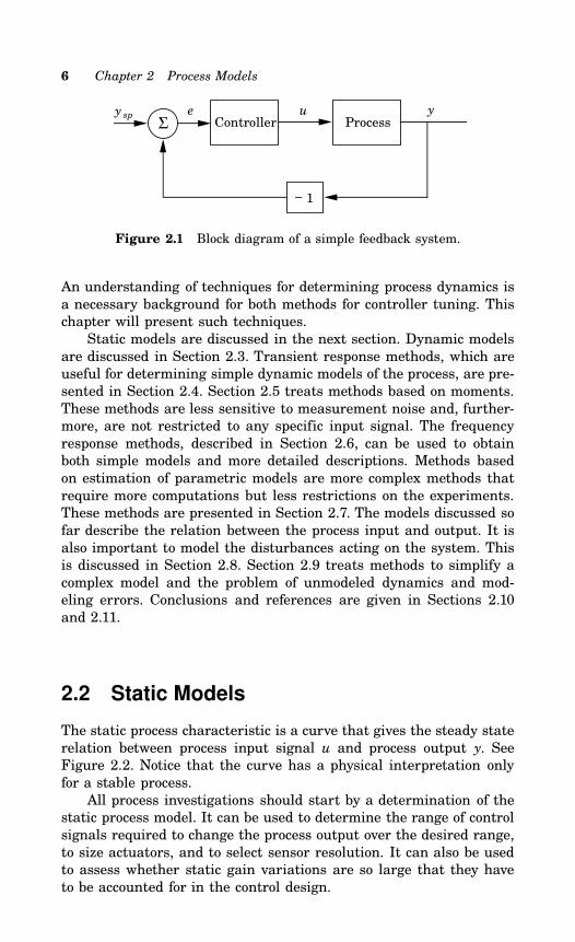
A block diagram of a simple control loop is shown in Figure 2.1. Thesystem has two major components, the process and the controller, rep-resented as boxes with arrows denoting the causal relation betweeninputs and outputs. The process has one input, the manipulated vari-able, also called the control variable. It is denoted by u. The processoutput is called process variable (PV) and is denoted by y. This vari-able is measured by a sensor. The desired value of the process variableis called the setpoint (SP) or the reference value. It is denoted by ysp.The control error e is the difference between the setpoint and theprocess variable, i.e., e = ysp − y. The controller in Figure 2.1 hasone input, the error, and one output, the control variable. The figureshows that the process and the controller are connected in a closedfeedback loop.The purpose of the system is to keep the process variable close
to the desired value in spite of disturbances. This is achieved by thefeedback loop, which works as follows. Assume that the system is inequilibrium and that a disturbance occurs so that the process variablebecomes larger than the setpoint. The error is then negative and thecontroller output decreases which in turn causes the process outputto decrease. This type of feedback is called negative feedback, becausethe manipulated variable moves in direction opposite to the processvariable.The controller has several parameters that can be adjusted. The
control loop performs well if the parameters are chosen properly. Itperforms poorly otherwise, e.g., the system may become unstable.The procedure of finding the controller parameters is called tuning.This can be done in two different ways. One approach is to choosesome controller parameters, to observe the behavior of the feedbacksystem, and to modify the parameters until the desired behavior isobtained. Another approach is to first develop a mathematical modelthat describes the behavior of the process. The parameters of thecontroller are then determined using some method for control design.
5
6 Chapter 2 Process Models
Controller Processe u y
Σ
1−
y sp
Figure 2.1 Block diagram of a simple feedback system.
An understanding of techniques for determining process dynamics isa necessary background for both methods for controller tuning. Thischapter will present such techniques.Static models are discussed in the next section. Dynamic models
are discussed in Section 2.3. Transient response methods, which areuseful for determining simple dynamic models of the process, are pre-sented in Section 2.4. Section 2.5 treats methods based on moments.These methods are less sensitive to measurement noise and, further-more, are not restricted to any specific input signal. The frequencyresponse methods, described in Section 2.6, can be used to obtainboth simple models and more detailed descriptions. Methods basedon estimation of parametric models are more complex methods thatrequire more computations but less restrictions on the experiments.These methods are presented in Section 2.7. The models discussed sofar describe the relation between the process input and output. It isalso important to model the disturbances acting on the system. Thisis discussed in Section 2.8. Section 2.9 treats methods to simplify acomplex model and the problem of unmodeled dynamics and mod-eling errors. Conclusions and references are given in Sections 2.10and 2.11.
2.2 Static Models
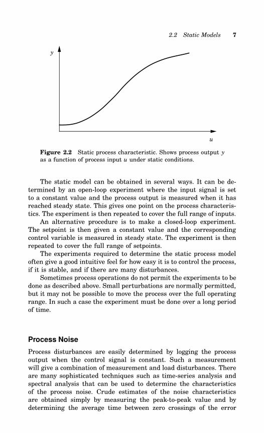
The static process characteristic is a curve that gives the steady staterelation between process input signal u and process output y. SeeFigure 2.2. Notice that the curve has a physical interpretation onlyfor a stable process.All process investigations should start by a determination of the
static process model. It can be used to determine the range of controlsignals required to change the process output over the desired range,to size actuators, and to select sensor resolution. It can also be usedto assess whether static gain variations are so large that they haveto be accounted for in the control design.
2.2 Static Models 7
y
u
Figure 2.2 Static process characteristic. Shows process output yas a function of process input u under static conditions.
The static model can be obtained in several ways. It can be de-termined by an open-loop experiment where the input signal is setto a constant value and the process output is measured when it hasreached steady state. This gives one point on the process characteris-tics. The experiment is then repeated to cover the full range of inputs.An alternative procedure is to make a closed-loop experiment.
The setpoint is then given a constant value and the correspondingcontrol variable is measured in steady state. The experiment is thenrepeated to cover the full range of setpoints.The experiments required to determine the static process model
often give a good intuitive feel for how easy it is to control the process,if it is stable, and if there are many disturbances.Sometimes process operations do not permit the experiments to be
done as described above. Small perturbations are normally permitted,but it may not be possible to move the process over the full operatingrange. In such a case the experiment must be done over a long periodof time.
Process Noise
Process disturbances are easily determined by logging the processoutput when the control signal is constant. Such a measurementwill give a combination of measurement and load disturbances. Thereare many sophisticated techniques such as time-series analysis andspectral analysis that can be used to determine the characteristicsof the process noise. Crude estimates of the noise characteristicsare obtained simply by measuring the peak-to-peak value and bydetermining the average time between zero crossings of the error
8 Chapter 2 Process Models
signal. This is discussed further in Section 2.8.
2.3 Dynamic Models
A static process model like the one discussed in the previous sectiontells the steady state relation between the input and the output signal.A dynamic model should give the relation between the input and theoutput signal during transients. It is naturally much more difficultto capture dynamic behavior. This is, however, very significant whendiscussing control problems.Fortunately there is a restricted class of models that can often be
used. This applies to linear time-invariant systems. Such models canoften be used to describe the behavior of control systems when thereare small deviations from an equilibrium. The fact that a system islinear implies that the superposition principle holds. This means thatif the input u1 gives the output y1 and the input u2 gives the outputy2 it then follows that the input au1 + bu2 gives the output ay1 + by2.A system is time-invariant if its behavior does not change with time.A very nice property of linear time-invariant systems is that their
response to an arbitrary input can be completely characterized interms of the response to a simple signal. Many different signals can beused to characterize a system. Broadly speaking we can differentiatebetween transient and frequency responses.In a control system we typically have to deal with two signals
only, the control signal and the measured variable. Process dynamicsas we have discussed here only deals with the relation between thosesignals. The measured variable should ideally be closely related to thephysical process variable that we are interested in. Since it is difficultto construct sensors it happens that there is considerable dynamicsin the relation between the true process variable and the sensor. Forexample, it is very common that there are substantial time constantsin temperature sensors. There may also be measurement noise andother imperfections. There may also be significant dynamics in theactuators. To do a good job of control, it is necessary to be aware ofthe physical origin the process dynamics to judge if a good responsein the measured variable actually corresponds to a good response inthe physical process variable.
Transient Responses
In transient response analysis the system dynamics are characterizedin terms of the response to a simple signal. The particular signal isoften chosen so that it is easy to generate experimentally. Typical
2.3 Dynamic Models 9
examples are steps, pulses, and impulses. Because of the superpo-sition principle the amplitude of the signals can be normalized. Forexample, it is sufficient to consider the response to a step with unitamplitude. If s(t) is the response to a unit step, the output y(t) to anarbitrary input signal u(t) is given by
y(t) =∫ t
−∞u(τ ) ds(t− τ )
dtdτ =
∫ t
−∞u(τ )h(t − τ )dτ (2.1)
where the impulse response h(t) is introduced as the time derivativeof the step response.In early process control literature the step response was also
called the reaction curve.Pulse response analysis is common in medical and biological ap-
plications, but rather uncommon in process control. Ramp responseanalysis is less common. One application is the determination of thederivative part of a PID controller. In process control, the step re-sponse is the most common transient used for process identification.This is primarily because this is the type of disturbance that is easi-est to generate manually. Step response methods are treated in detailin Section 2.4.
Frequency Response
Another way to characterize the dynamics of a linear time-invariantsystem is to use sine waves as a test signal. This idea goes backto Fourier. The idea is that the dynamics can be characterized byinvestigating how sine waves propagate through a system.Consider a stable linear system. If the input signal to the system
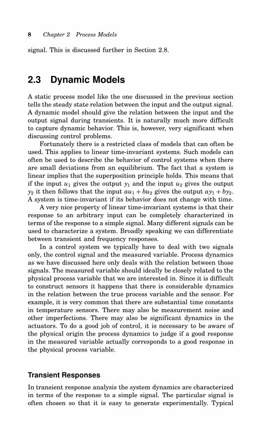
is a sinusoid, then the output signal will also be a sinusoid after atransient (see Figure 2.3). The output will have the same frequency asthe input signal. Only the phase and the amplitude are different. Thismeans that under stationary conditions, the relationship between theinput and the output can be described by two numbers: the quotient(a) between the input and the output amplitude, and the phase shift(ϕ) between the input and the output signals. The functions a(ω ) andϕ(ω ) describe a and ϕ for all frequencies (ω ). It is convenient to viewa and ϕ as the magnitude and the argument of a complex number
G(iω ) = a(ω )eiϕ (ω ) (2.2)The function G(iω ) is called the frequency response function of thesystem. The function a(ω ) = G(iω ) is called the amplitude function,and the function ϕ(ω ) = ar(G(iω )) is called the phase function.The complex number G(iω ) can be represented by a vector with
length a(iω ) that forms angle ϕ(iω ) with the real axis (see Figure
10 Chapter 2 Process Models
0 5 10 15
0
0.1
0 5 10 15
−1
1
y
u
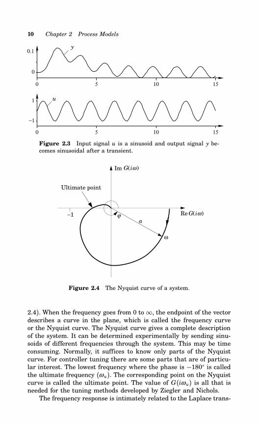
Figure 2.3 Input signal u is a sinusoid and output signal y be-comes sinusoidal after a transient.
ω
ϕ−1
Ultimate point
a G(iω) Re
G(iω) Im
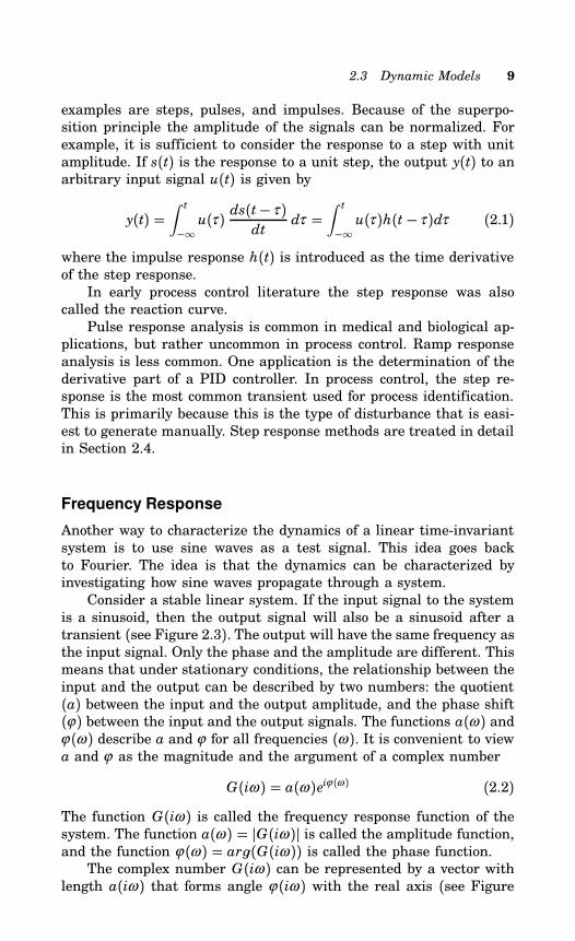
Figure 2.4 The Nyquist curve of a system.
2.4). When the frequency goes from 0 to∞, the endpoint of the vectordescribes a curve in the plane, which is called the frequency curveor the Nyquist curve. The Nyquist curve gives a complete descriptionof the system. It can be determined experimentally by sending sinu-soids of different frequencies through the system. This may be timeconsuming. Normally, it suffices to know only parts of the Nyquistcurve. For controller tuning there are some parts that are of particu-lar interest. The lowest frequency where the phase is −180 is calledthe ultimate frequency (ωu). The corresponding point on the Nyquistcurve is called the ultimate point. The value of G(iωu) is all that isneeded for the tuning methods developed by Ziegler and Nichols.The frequency response is intimately related to the Laplace trans-
2.4 Step Response Methods 11
form. Let f (t) be a signal. The Laplace transform of the signal, F(s),is then defined by
F(s) =∫ ∞
0e−st f (t)dt (2.3)
Let U (s) and Y(s) be the Laplace transforms of the input and theoutput of a linear time-invariant dynamical system. Assume that thesystem is at rest at time t = 0. The following relation then holds
Y(s) = G(s)U (s) (2.4)where G(s) is the transfer function of the system.It follows from Equation (2.3) that the Laplace transform of an
impulse is 1. From Equation (2.4) we can conclude that G(s) is theLaplace transform of the impulse response. The frequency responseis simply G(iω ).In the following sections we will show how linear system dynamics
can be obtained experimentally. We will illustrate both transient andfrequency response methods.
2.4 Step Response Methods
The dynamics of a process can be determined from the response ofthe process to pulses, steps, ramps, or other deterministic signals.The dynamics of a linear system is, in principle, uniquely given fromsuch a transient response experiment. This requires, however, thatthe system is at rest before the input is applied, and that there are nomeasurement errors. In practice, however, it is difficult to ensure thatthe system is at rest. There will also be measurement errors, so thetransient response method, in practice, is limited to the determinationof simple models. Models obtained from a transient experiment are,however, often sufficient for PID controller tuning. The methods arealso very simple to use. This section focuses on the step responsemethod.
The Step Response
Assuming a control loop with a controller, the step response experi-ment can be determined as follows. Wait until the process is at rest.Set the controller to manual. Change the control variable rapidly, e.g.,through the use of increase/decrease buttons. Record the process vari-able and scale it by dividing by the change in the control variable.The change in control variable should be as large as possible in orderto get a maximum signal to noise ratio. The limit is set by permissible
12 Chapter 2 Process Models
0 2 4 6 80
0.4
0.8
0 2 4 6 80
0.4
0 2 4 6 80
0.4
0.8
0 2 4 6 80
1
0 2 4 6 80
2
0 2 4 6 8
−0.5
0.5
A
C
E
B
D
F
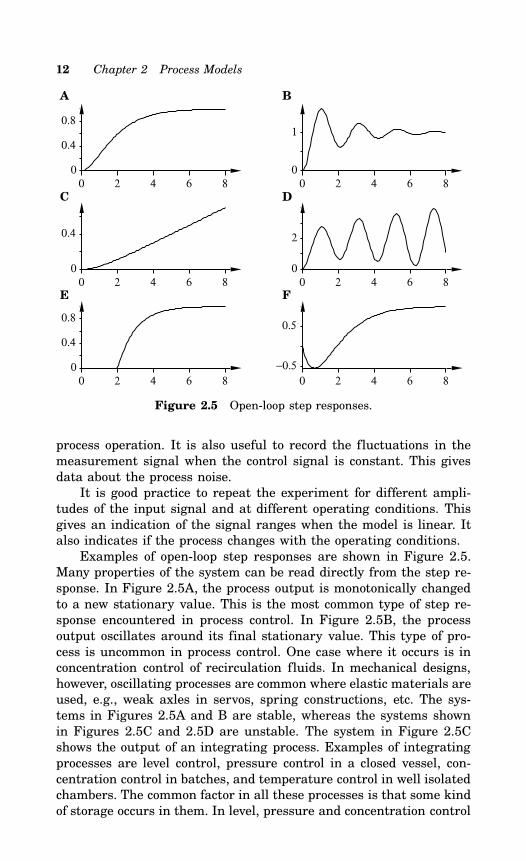
Figure 2.5 Open-loop step responses.
process operation. It is also useful to record the fluctuations in themeasurement signal when the control signal is constant. This givesdata about the process noise.It is good practice to repeat the experiment for different ampli-
tudes of the input signal and at different operating conditions. Thisgives an indication of the signal ranges when the model is linear. Italso indicates if the process changes with the operating conditions.Examples of open-loop step responses are shown in Figure 2.5.
Many properties of the system can be read directly from the step re-sponse. In Figure 2.5A, the process output is monotonically changedto a new stationary value. This is the most common type of step re-sponse encountered in process control. In Figure 2.5B, the processoutput oscillates around its final stationary value. This type of pro-cess is uncommon in process control. One case where it occurs is inconcentration control of recirculation fluids. In mechanical designs,however, oscillating processes are common where elastic materials areused, e.g., weak axles in servos, spring constructions, etc. The sys-tems in Figures 2.5A and B are stable, whereas the systems shownin Figures 2.5C and 2.5D are unstable. The system in Figure 2.5Cshows the output of an integrating process. Examples of integratingprocesses are level control, pressure control in a closed vessel, con-centration control in batches, and temperature control in well isolatedchambers. The common factor in all these processes is that some kindof storage occurs in them. In level, pressure and concentration control
2.4 Step Response Methods 13
storage of mass occurs, while in the case of temperature control thereis a storage of energy. The system in Figure 2.5E has a long deadtime. The dead time occurs when there are transportation delays inthe process. The system in Figure 2.5F is a non-minimum phase sys-tem, where the measurement signal initially moves in the “wrong”direction. The water level in boilers often reacts like this after a stepchange in feed water flow.If the system is linear, all step responses are proportional to
the size of the step in the input signal. It is then convenient tonormalize the responses by dividing the measurement signal by thestep size of the control signal. Throughout this book we assume thatthis normalization is done.The step response is a convenient way to characterize process
dynamics because of its simple physical interpretation. Many tuningmethods are based on it. A formal mathematical model can also beobtained from the step response. General methods for the design ofcontrol systems can then be used.For small perturbations the static process model can be described
by one parameter called the process gain. This is simply the ratio ofthe steady state changes of process output and process input. The gaincan be obtained as the slope of the curve in Figure 2.2. It can alsobe obtained directly from a step response. For nonlinear systems theprocess gain will depend on the operating conditions. It is, however,constant for linear systems. For such systems the static properties arethus described by one parameter. Additional parameters are neededto also capture dynamics. Some simple parametric models will bedescribed below. Stable processes with a monotone step response, asshown in Figure 2.5A, are quite common. Many methods to obtainparametric models from such a step response have been presented inthe literature over the years. We will present here models with two,three, and, four parameters respectively.
Two-Parameter Models
The simplest parametric models of process dynamics have two param-eters. One parameter can be process gain. The other has to capturethe time behavior. The average residence time Tar is a useful param-eter. This is obtained as
Tar = A0K
where K is the static process gain and A0 is defined as
A0 =∞∫0
(s(∞) − s(t))dt
14 Chapter 2 Process Models
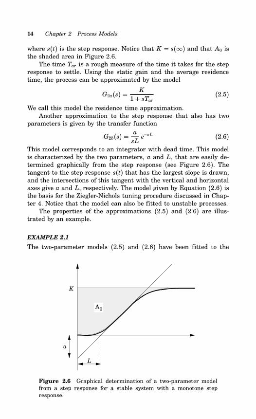
where s(t) is the step response. Notice that K = s(∞) and that A0 isthe shaded area in Figure 2.6.The time Tar is a rough measure of the time it takes for the step
response to settle. Using the static gain and the average residencetime, the process can be approximated by the model
G2a(s) = K
1+ sTar (2.5)We call this model the residence time approximation.Another approximation to the step response that also has two
parameters is given by the transfer function
G2b(s) = a
sLe−sL (2.6)
This model corresponds to an integrator with dead time. This modelis characterized by the two parameters, a and L, that are easily de-termined graphically from the step response (see Figure 2.6). Thetangent to the step response s(t) that has the largest slope is drawn,and the intersections of this tangent with the vertical and horizontalaxes give a and L, respectively. The model given by Equation (2.6) isthe basis for the Ziegler-Nichols tuning procedure discussed in Chap-ter 4. Notice that the model can also be fitted to unstable processes.The properties of the approximations (2.5) and (2.6) are illus-
trated by an example.
EXAMPLE 2.1
The two-parameter models (2.5) and (2.6) have been fitted to the
a
L
K
A0
Figure 2.6 Graphical determination of a two-parameter modelfrom a step response for a stable system with a monotone stepresponse.
2.4 Step Response Methods 15
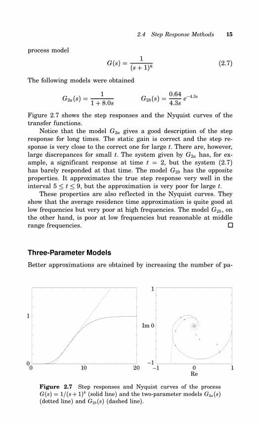
process model
G(s) = 1(s+ 1)8 (2.7)
The following models were obtained
G2a(s) = 11+ 8.0s G2b(s) = 0.644.3s e
−4.3s
Figure 2.7 shows the step responses and the Nyquist curves of thetransfer functions.Notice that the model G2a gives a good description of the step
response for long times. The static gain is correct and the step re-sponse is very close to the correct one for large t. There are, however,large discrepances for small t. The system given by G2a has, for ex-ample, a significant response at time t = 2, but the system (2.7)has barely responded at that time. The model G2b has the oppositeproperties. It approximates the true step response very well in theinterval 5 ≤ t ≤ 9, but the approximation is very poor for large t.These properties are also reflected in the Nyquist curves. They
show that the average residence time approximation is quite good atlow frequencies but very poor at high frequencies. The model G2b, onthe other hand, is poor at low frequencies but reasonable at middlerange frequencies.
Three-Parameter Models
Better approximations are obtained by increasing the number of pa-
x
x
x
x
x
x
x
x
0 10 20 –1 0 10
1
–1
0
1
Re
Im
Figure 2.7 Step responses and Nyquist curves of the processG(s) = 1/(s+ 1)8 (solid line) and the two-parameter models G2a(s)(dotted line) and G2b(s) (dashed line).
16 Chapter 2 Process Models
rameters. The model
G(s) = K
1+ sT e−sL (2.8)
is characterized by three parameters: the static gain K , the timeconstant T , and the dead time L. This is the most common processmodel used in papers on PID controller tuning. The parameters Land T are often called the apparent dead time and the apparent timeconstant, respectively. The step response of the model (2.8) is
s(t) = K(1− e−(t−L)/T
)From this equation, it follows that the average residence time is
Tar =
∞∫0(s(∞) − s(t))dt
K= L + T
The ratio
τ = L
L + T =L
Tar(2.9)
which has the property 0 ≤ τ ≤ 1, is called the normalized dead time.This quantity can be used to characterize the difficulty of controllinga process. It is sometimes also called the controllability ratio. Roughlyspeaking, it has been found that processes with small τ are easy tocontrol and that the difficulty in controlling the system increasesas τ increases. Systems with τ = 1 correspond to pure dead-timeprocesses, which are indeed difficult to control well.The parameters in the model (2.8) can be determined graphically.
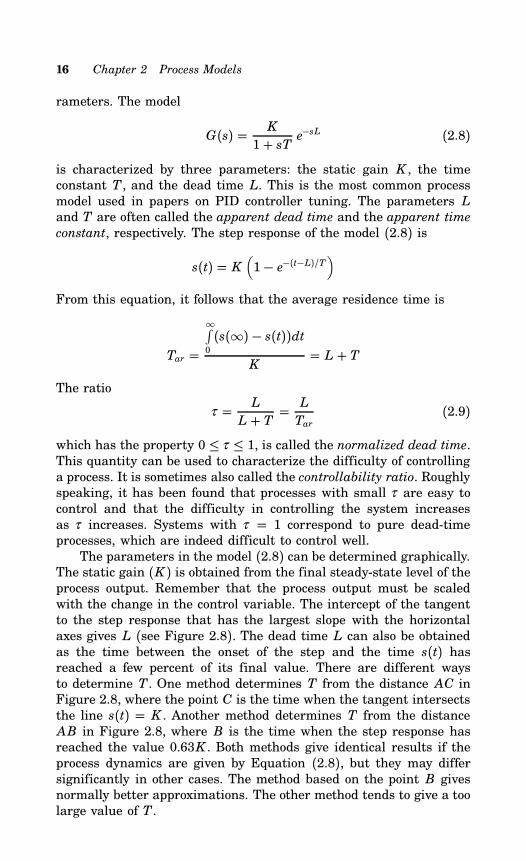
The static gain (K ) is obtained from the final steady-state level of theprocess output. Remember that the process output must be scaledwith the change in the control variable. The intercept of the tangentto the step response that has the largest slope with the horizontalaxes gives L (see Figure 2.8). The dead time L can also be obtainedas the time between the onset of the step and the time s(t) hasreached a few percent of its final value. There are different waysto determine T . One method determines T from the distance AC inFigure 2.8, where the point C is the time when the tangent intersectsthe line s(t) = K . Another method determines T from the distanceAB in Figure 2.8, where B is the time when the step response hasreached the value 0.63K . Both methods give identical results if theprocess dynamics are given by Equation (2.8), but they may differsignificantly in other cases. The method based on the point B givesnormally better approximations. The other method tends to give a toolarge value of T .
2.4 Step Response Methods 17
L B
0.63 K
A C
K
Figure 2.8 Graphical determination of three-parameter modelsfor systems with a monotone step response.
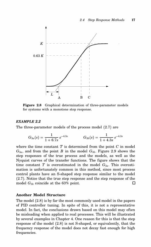
EXAMPLE 2.2
The three-parameter models of the process model (2.7) are
G3a(s) = 11+ 6.7s e
−4.3s G3b(s) = 11+ 4.3s e
−4.3s
where the time constant T is determined from the point C in modelG3a, and from the point B in the model G3b. Figure 2.9 shows thestep responses of the true process and the models, as well as theNyquist curves of the transfer functions. The figure shows that thetime constant T is overestimated in the model G3a. This overesti-mation is unfortunately common in this method, since most processcontrol plants have an S-shaped step response similar to the model(2.7). Notice that the true step response and the step response of themodel G3b coincide at the 63% point.
Another Model Structure
The model (2.8) is by far the most commonly used model in the papersof PID controller tuning. In spite of this, it is not a representativemodel. In fact, the conclusions drawn based on this model may oftenbe misleading when applied to real processes. This will be illustratedby several examples in Chapter 4. One reason for this is that the stepresponse of the model (2.8) is not S-shaped, or equivalently, that thefrequency response of the model does not decay fast enough for highfrequencies.
18 Chapter 2 Process Models
x
x
x
x
x
x
x
x
x
0 10 20 –1 0 10
1
–1
0
1
Re
Im
Figure 2.9 Step responses and Nyquist curves of the processG(s) = 1/(s+1)8 (solid line) and the three-parameter models G3a(s)(dashed line) and G3b(s) (dotted line).
Another three-parameter model is
G(s) = K
(1+ sT)2 e−sL (2.10)
The step response of this model is
s(t) = K(1−
(1+ t− L
T
)e−(t−L)/T
)(2.11)
This model has an S-shaped step response and often gives a betterapproximation than the first-order plus dead-time model (2.8). Staticgain K and dead time L can be determined in the same way asfor the model (2.8). Time constant T can then be determined fromEquation 2.11 if the value of the step response at one time is known.The equation obtained must be solved numerically.
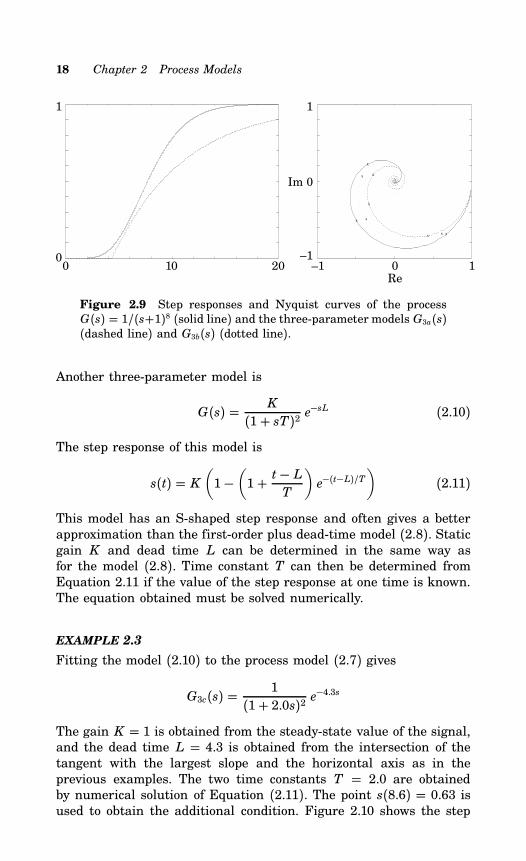
EXAMPLE 2.3
Fitting the model (2.10) to the process model (2.7) gives
G3c(s) = 1(1+ 2.0s)2 e
−4.3s
The gain K = 1 is obtained from the steady-state value of the signal,and the dead time L = 4.3 is obtained from the intersection of thetangent with the largest slope and the horizontal axis as in theprevious examples. The two time constants T = 2.0 are obtainedby numerical solution of Equation (2.11). The point s(8.6) = 0.63 isused to obtain the additional condition. Figure 2.10 shows the step
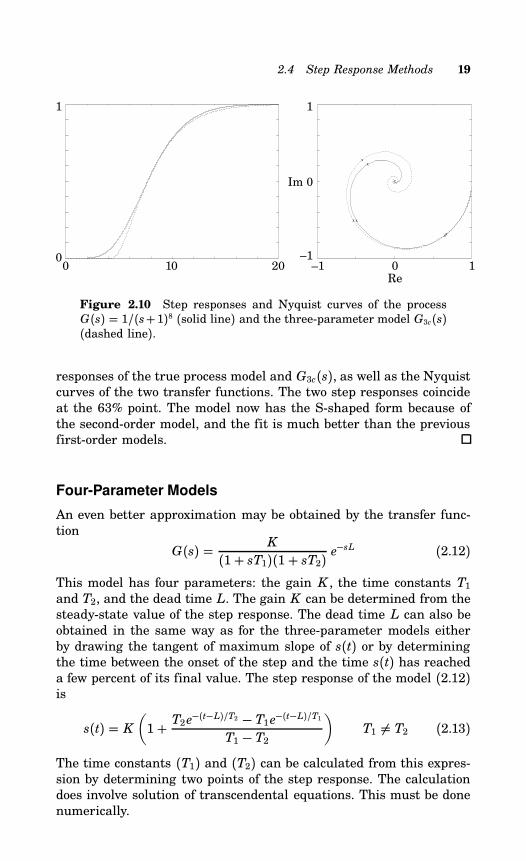
2.4 Step Response Methods 19
x
x
x
x
x
x
0 10 20 –1 0 10
1
–1
0
1
Re
Im
Figure 2.10 Step responses and Nyquist curves of the processG(s) = 1/(s+1)8 (solid line) and the three-parameter model G3c(s)(dashed line).
responses of the true process model and G3c(s), as well as the Nyquistcurves of the two transfer functions. The two step responses coincideat the 63% point. The model now has the S-shaped form because ofthe second-order model, and the fit is much better than the previousfirst-order models.
Four-Parameter Models
An even better approximation may be obtained by the transfer func-tion
G(s) = K
(1+ sT1)(1+ sT2) e−sL (2.12)
This model has four parameters: the gain K , the time constants T1and T2, and the dead time L. The gain K can be determined from thesteady-state value of the step response. The dead time L can also beobtained in the same way as for the three-parameter models eitherby drawing the tangent of maximum slope of s(t) or by determiningthe time between the onset of the step and the time s(t) has reacheda few percent of its final value. The step response of the model (2.12)is
s(t) = K(1+ T2e
−(t−L)/T2 − T1e−(t−L)/T1T1 − T2
)T1 = T2 (2.13)
The time constants (T1) and (T2) can be calculated from this expres-sion by determining two points of the step response. The calculationdoes involve solution of transcendental equations. This must be donenumerically.
20 Chapter 2 Process Models
x
x
x
x
x
x
0 10 20 –1 0 10
1
–1
0
1
Re
Im
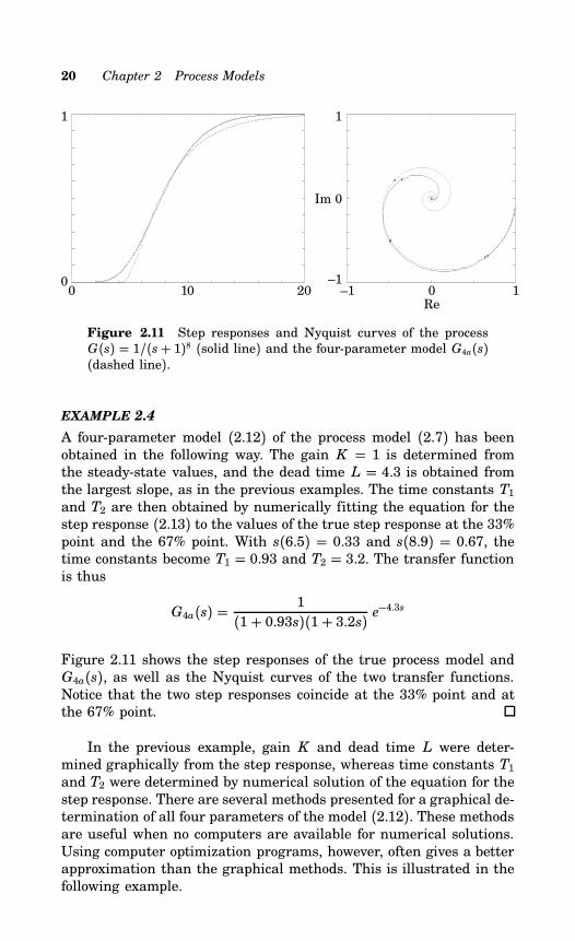
Figure 2.11 Step responses and Nyquist curves of the processG(s) = 1/(s+ 1)8 (solid line) and the four-parameter model G4a(s)(dashed line).
EXAMPLE 2.4
A four-parameter model (2.12) of the process model (2.7) has beenobtained in the following way. The gain K = 1 is determined fromthe steady-state values, and the dead time L = 4.3 is obtained fromthe largest slope, as in the previous examples. The time constants T1and T2 are then obtained by numerically fitting the equation for thestep response (2.13) to the values of the true step response at the 33%point and the 67% point. With s(6.5) = 0.33 and s(8.9) = 0.67, thetime constants become T1 = 0.93 and T2 = 3.2. The transfer functionis thus
G4a(s) = 1(1+ 0.93s)(1+ 3.2s) e
−4.3s
Figure 2.11 shows the step responses of the true process model andG4a(s), as well as the Nyquist curves of the two transfer functions.Notice that the two step responses coincide at the 33% point and atthe 67% point.
In the previous example, gain K and dead time L were deter-mined graphically from the step response, whereas time constants T1and T2 were determined by numerical solution of the equation for thestep response. There are several methods presented for a graphical de-termination of all four parameters of the model (2.12). These methodsare useful when no computers are available for numerical solutions.Using computer optimization programs, however, often gives a betterapproximation than the graphical methods. This is illustrated in thefollowing example.
2.4 Step Response Methods 21
x
x
x
x
x
x
0 10 20 –1 0 10
1
–1
0
1
Re
Im
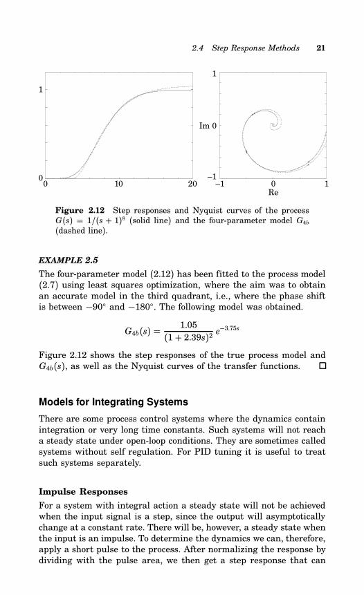
Figure 2.12 Step responses and Nyquist curves of the processG(s) = 1/(s + 1)8 (solid line) and the four-parameter model G4b(dashed line).
EXAMPLE 2.5
The four-parameter model (2.12) has been fitted to the process model(2.7) using least squares optimization, where the aim was to obtainan accurate model in the third quadrant, i.e., where the phase shiftis between −90 and −180. The following model was obtained.
G4b(s) = 1.05(1+ 2.39s)2 e
−3.75s
Figure 2.12 shows the step responses of the true process model andG4b(s), as well as the Nyquist curves of the transfer functions.
Models for Integrating Systems
There are some process control systems where the dynamics containintegration or very long time constants. Such systems will not reacha steady state under open-loop conditions. They are sometimes calledsystems without self regulation. For PID tuning it is useful to treatsuch systems separately.
Impulse Responses
For a system with integral action a steady state will not be achievedwhen the input signal is a step, since the output will asymptoticallychange at a constant rate. There will be, however, a steady state whenthe input is an impulse. To determine the dynamics we can, therefore,apply a short pulse to the process. After normalizing the response bydividing with the pulse area, we then get a step response that can
22 Chapter 2 Process Models
be modeled using the methods we have just discussed. The transferfunction of a system with integral action is then obtained simply bymultiplying the transfer function by 1/s. We illustrate the procedurewith an example.
EXAMPLE 2.6
Assume that a square pulse with unit height and duration τ has beenapplied to a process and that the model
G1(s) = K
1+ sT e−sL
has been fitted to the response as described in Example 2.2. Thetransfer function of the process is then
G(s) = 1sτG1(s) = K
sτ (1+ sT) e−sL
Step Responses
Models based on step responses can also be applied to processes withintegral action. One possibility is to calculate the derivative of thestep response and apply the impulse response method that was justdiscussed.The two-parameter model
G(s) = a
sLe−sL
that was used to model stable processes previously in this sectioncan also be applied to integrating processes. This model gives a baddescription of stable processes at high frequencies, but for integratingprocesses the low frequency behavior is well captured by the model.A more sophisticated model that gives a better approximation at
higher frequencies is given by the transfer function
G(s) = K
s(1+ sT) e−sL (2.14)
The model is characterized by three parameters: the velocity gain K ,the time constant T , and the dead time L. The step response of themodel (2.14) is
s(t) = K(t− L− T
(1− e−(t−L)/T
))(2.15)
The gain K and the average residence time Tar = L + T can bedetermined graphically as shown in Figure 2.13.
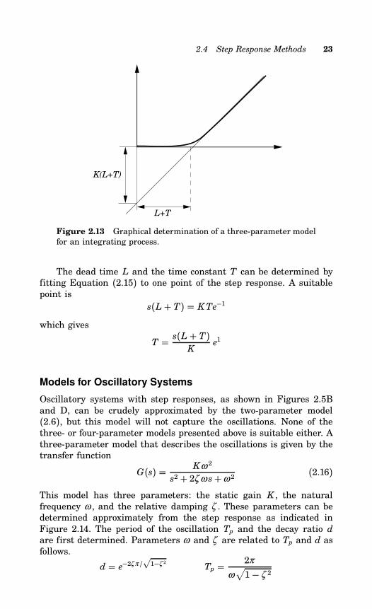
2.4 Step Response Methods 23
K(L+T)
L+T
Figure 2.13 Graphical determination of a three-parameter modelfor an integrating process.
The dead time L and the time constant T can be determined byfitting Equation (2.15) to one point of the step response. A suitablepoint is
s(L+ T) = KTe−1
which gives
T = s(L+ T)K
e1
Models for Oscillatory Systems
Oscillatory systems with step responses, as shown in Figures 2.5Band D, can be crudely approximated by the two-parameter model(2.6), but this model will not capture the oscillations. None of thethree- or four-parameter models presented above is suitable either. Athree-parameter model that describes the oscillations is given by thetransfer function
G(s) = Kω 2
s2 + 2ζ ω s+ω 2(2.16)
This model has three parameters: the static gain K , the naturalfrequency ω , and the relative damping ζ . These parameters can bedetermined approximately from the step response as indicated inFigure 2.14. The period of the oscillation Tp and the decay ratio dare first determined. Parameters ω and ζ are related to Tp and d asfollows.
d = e−2ζ π /√1−ζ 2 Tp = 2π
ω√1− ζ 2
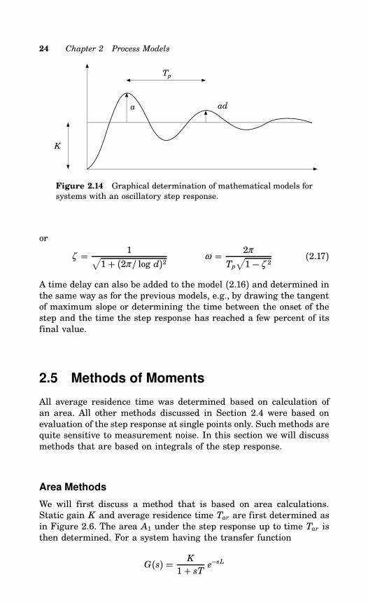
24 Chapter 2 Process Models
K
a ad
Tp
Figure 2.14 Graphical determination of mathematical models forsystems with an oscillatory step response.
or
ζ = 1√1+ (2π/ log d)2 ω = 2π
Tp√1− ζ 2
(2.17)
A time delay can also be added to the model (2.16) and determined inthe same way as for the previous models, e.g., by drawing the tangentof maximum slope or determining the time between the onset of thestep and the time the step response has reached a few percent of itsfinal value.
2.5 Methods of Moments
All average residence time was determined based on calculation ofan area. All other methods discussed in Section 2.4 were based onevaluation of the step response at single points only. Such methods arequite sensitive to measurement noise. In this section we will discussmethods that are based on integrals of the step response.
Area Methods
We will first discuss a method that is based on area calculations.Static gain K and average residence time Tar are first determined asin Figure 2.6. The area A1 under the step response up to time Tar isthen determined. For a system having the transfer function
G(s) = K
1+ sT e−sL
2.5 Methods of Moments 25
we have
A1 =Tar∫0
s(t)dt =T∫0
K (1− e−t/T)dt = KTe−1
The time constant is thus given by
T = eA1K
(2.18)
The dead time is then given by
L = Tar − T = A0K− eA1K
(2.19)
With this method parameters L and T are both determined fromcomputations of areas. The method is illustrated by the followingexample.
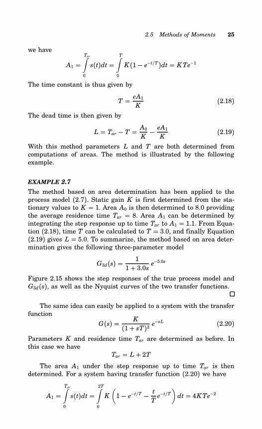
EXAMPLE 2.7
The method based on area determination has been applied to theprocess model (2.7). Static gain K is first determined from the sta-tionary values to K = 1. Area A0 is then determined to 8.0 providingthe average residence time Tar = 8. Area A1 can be determined byintegrating the step response up to time Tar to A1 = 1.1. From Equa-tion (2.18), time T can be calculated to T = 3.0, and finally Equation(2.19) gives L = 5.0. To summarize, the method based on area deter-mination gives the following three-parameter model
G3d(s) = 11+ 3.0s e
−5.0s
Figure 2.15 shows the step responses of the true process model andG3d(s), as well as the Nyquist curves of the two transfer functions.
The same idea can easily be applied to a system with the transferfunction
G(s) = K
(1+ sT)2 e−sL (2.20)
Parameters K and residence time Tar are determined as before. Inthis case we have
Tar = L+ 2TThe area A1 under the step response up to time Tar is then
determined. For a system having transfer function (2.20) we have
A1 =Tar∫0
s(t)dt =2T∫0
K
(1− e−t/T − t
Te−t/T
)dt = 4KTe−2
26 Chapter 2 Process Models
x
x
x
x
x
x
0 10 20 –1 0 10
1
–1
0
1
Re
Im
Figure 2.15 Step responses and Nyquist curves of the processG(s) = 1/(s+1)8 (solid line) and the three-parameter model G3d(s)(dashed line).
The time constant is thus given by
T = A1e2
4K(2.21)
and the dead time is
L = Tar − 2T = A0K− A1e
2
2K(2.22)
The following example illustrates the properties of the method.
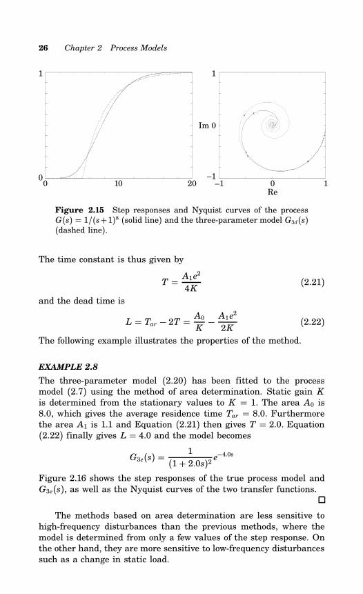
EXAMPLE 2.8
The three-parameter model (2.20) has been fitted to the processmodel (2.7) using the method of area determination. Static gain Kis determined from the stationary values to K = 1. The area A0 is8.0, which gives the average residence time Tar = 8.0. Furthermorethe area A1 is 1.1 and Equation (2.21) then gives T = 2.0. Equation(2.22) finally gives L = 4.0 and the model becomes
G3e(s) = 1(1+ 2.0s)2 e
−4.0s
Figure 2.16 shows the step responses of the true process model andG3e(s), as well as the Nyquist curves of the two transfer functions.
The methods based on area determination are less sensitive tohigh-frequency disturbances than the previous methods, where themodel is determined from only a few values of the step response. Onthe other hand, they are more sensitive to low-frequency disturbancessuch as a change in static load.
2.5 Methods of Moments 27
x
x
x
x
x
x
0 10 20 –1 0 10
1
–1
0
1
Re
Im
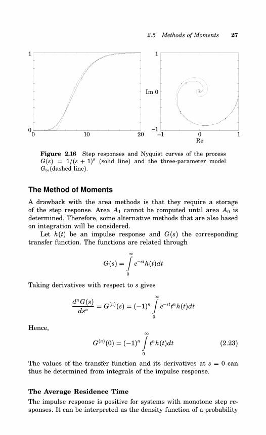
Figure 2.16 Step responses and Nyquist curves of the processG(s) = 1/(s + 1)8 (solid line) and the three-parameter modelG3e(dashed line).
The Method of Moments
A drawback with the area methods is that they require a storageof the step response. Area A1 cannot be computed until area A0 isdetermined. Therefore, some alternative methods that are also basedon integration will be considered.Let h(t) be an impulse response and G(s) the corresponding
transfer function. The functions are related through
G(s) =∞∫0
e−sth(t)dt
Taking derivatives with respect to s gives
dnG(s)dsn
= G(n)(s) = (−1)n∞∫0
e−sttnh(t)dt
Hence,
G(n)(0) = (−1)n∞∫0
tnh(t)dt (2.23)
The values of the transfer function and its derivatives at s = 0 canthus be determined from integrals of the impulse response.
The Average Residence Time
The impulse response is positive for systems with monotone step re-sponses. It can be interpreted as the density function of a probability
28 Chapter 2 Process Models
distribution if it is normalized as follows:
f (t) = h(t)∞∫0h(t)dt
The quantity f (t)dt can then be interpreted as the probability thatan impulse entering the system at time 0 will leave at time t. Theaverage residence time is then
Tar =∞∫0
t f (t)dt =
∞∫0th(t)dt∞∫0h(t)dt
(2.24)
Introduce(t) = s(∞) − s(t)
where s(t) is the unit step response. Thend(t)dt
= −h(t)
It follows that∞∫0
th(t)dt =[−t(t)
]∞0+∞∫0
(t)dt
The first term of the right-hand side is zero if (t) goes to zero atleast as fast as t1+ε for large t. The average residence time can thusalso be written as
Tar =
∞∫0(s(∞) − s(t))dt
s(∞)which is the definition used previously.Equation (2.23) gives a convenient way to determine parameters
of different models by computing the moments. This will be illustratedby some examples.
A Three-Parameter Model
Consider the transfer function
G(s) = K
1+ sT e−sL (2.25)
It follows that
K = G(0) =∞∫0
h(t)dt (2.26)
2.5 Methods of Moments 29
Taking logarithms of Equation (2.25) giveslogG(s) = log K − sL− log (1+ sT)
Differentiating this expression gives
G ′(s)G(s) = −L −
T
1+ sTG ′′(s)G(s) −
(G ′(s)G(s)
)2= T2
(1+ sT)2Hence
Tar = −G′(0)G(0) = L+ T =
∞∫0th(t)dt∞∫0h(t)dt
T2 = G′′(0)G(0) − T
2ar =
∞∫0t2h(t)dt∞∫0h(t)dt
− T2ar
(2.27)
Gain K is thus given by Equation (2.26) and average residence timeTar and time constant T by Equation (2.27). The dead time L canthen be computed to
L = Tar − TIt has thus been shown that the parameters of the model can beobtained from the first two moments of the impulse response. Weillustrate the procedure with an example.
EXAMPLE 2.9
Consider the process model
G(s) = 1(s+ 1)8
The first two derivatives with respect to s become
G ′(s) = − 8(s+ 1)9 G ′′(s) = 72
(s+ 1)10
Hence G(0) = 1, G ′(0) = −8, and G ′′(0) = 72. Equations (2.26) and(2.27) now give
K = 1Tar = 8T2 = 72− 64 = 8
30 Chapter 2 Process Models
We thus find T = 2√2 2.8 and L = 8− 2√2 5.2. This result canbe compared with the previous methods in Examples 2.2 and 2.7.
Another Three-Parameter Model
The method of moments will now be applied to determine the param-eters of the transfer function
G(s) = K
(1+ sT)2 e−sL
We havelogG(s) = log K − sL− 2 log (1+ sT)
HenceG ′(s)G(s) = −L −
2T1+ sT
G ′′(s)G(s) −
(G ′(s)G(s)
)2= 2T2
(1+ sT)2Hence
K = G(0) =∞∫0
h(t)dt
Tar = −G′(0)G(0) = L+ 2T =
∞∫0th(t)dt∞∫0h(t)dt
T2 = G′′(0)2G(0) −
12T2ar =
∞∫0t2h(t)dt
2∞∫0h(t)dt
− 12T2ar
(2.28)
We illustrate the method with an example.
EXAMPLE 2.10
Consider the process model (2.7). It follows from the previous examplethat G(0) = 1, G ′(0) = −8, and G ′′(0) = 72. We thus find K = 1,Tar = 8, T = 2 and L = 4. This is the same model as the one obtainedin Example 2.8.
Other Input Signals
From a practical point of view it is a drawback to have methods thatrequire special input signals. The method of moments can be appliedto any signal provided that the system is initially at rest.
2.5 Methods of Moments 31
Let U (s) and Y(s) be the Laplace transforms of an arbitrary inputand the corresponding output, respectively. Taking derivatives we get
Y(s) = G(s)U (s)Y ′(s) = G ′(s)U (s) + G(s)U ′(s)Y ′′(s) = G ′′(s)U (s) + 2G ′(s)U ′(s) + G(s)U ′′(s)
etc.
Hence,
Y(0) = G(0)U (0)Y ′(0) = G ′(0)U (0) + G(0)U ′(0)Y ′′(0) = G ′′(0)U (0) + 2G ′(0)U ′(0) + G(0)U ′′(0)
etc.
(2.29)
The transfer function G(0) and its derivatives can thus be calculatedfrom experiments with arbitrary inputs by calculating the followingmoments of the input and output
U (n)(0) = (−1)n∞∫0
tnu(t)dt
Y(n)(0) = (−1)n∞∫0
tny(t)dt
and using Equation (2.29).By using these formulas it is possible to calculate G(n)(0) for any
signals for which the moments
un =∞∫0
tnu(t)dt
and
yn =∞∫0
tny(t)dt
exist. This means that the signals must decay sufficiently fast.A typical case where the method can be used is when an exper-
iment is performed in a closed loop with a pulse-like perturbationsignal on the process input.
32 Chapter 2 Process Models
Weighted Moments
The method just discussed cannot be used if the signals do not goto zero or, equivalently, to a priori known mean values that can besubtracted in the calculations of moments, because the moments willthen be infinite. There is, however, a simple modification that canbe used in this case. It follows from the definition of the Laplacetransform that
Y(n)(s) = dnY(s)dsn
= (−1)n∞∫0
e−sttny(t)dt
The weighted moments
yn =∞∫0
tne−α ty(t)dt = (−1)nY(n)(α )
will exist provided that y(t) does not grow faster than eα t for larget. By computing yn and the analogously defined moment un, we cancompute Y(n)(α ) and U (n)(α ), and thus also G(n)(α ).
A Three-Parameter Model
Consider a system with the transfer function
G(s) = K
1+ sT e−sL (2.30)
We havelogG(s) = log K − sL− log (1+ sT)
HenceG ′(s)G(s) = −L −
T
1+ sTG ′′(s)G(s) −
(G ′(s)G(s)
)2= T2
(1+ sT)2Thus we get
T2
(1+αT)2 =G ′′(α )G(α ) −
(G ′(α )G(α )
)2= a2 (2.31)
Hence,
T = a
1−α a
L = −G′(α )G(α ) − a
(2.32)
2.5 Methods of Moments 33
The average residence time thus becomes
Tar = L + T = −G′(α )G(α ) +
α a2
1−α a
Furthermore the static gain is given by
K = (1+αT)G(α )eα L (2.33)
The formulas are illustrated by an example.
EXAMPLE 2.11
Consider a system with the transfer function
G(s) = 1(s+ 1)8
We have
G(α ) = 1(1+α )8 G ′(α ) = −8
(1+α )9 G ′′(α ) = 72(1+α )10
Computing the derivatives at the origin from the first terms in theTaylor series expansion gives
G(0) 1(1+α )8 +
8α(1+α )9 =
1+ 9α(1+α )9
G ′(0) − 8(1 +α )9 −
72α(1+α )10 = −
8(1+ 10α )(1+α )10
The estimate of the average residence time becomes
Tar = −G′(0)G(0)
8(1+ 10α )(1+α )(1+ 9α ) =
8(1+ 10α )1+ 10α + 9α 2
From these expressions it follows that α must be small in order togive reasonably good approximations. To discuss the values of α , it isreasonable to normalize and consider αTar. In this case, Tar = 8. WithαTar = 1 we get G(0) = 0.74, G ′(0) = −5.54, and Tar = 7.53. WithαTar = 0.5 we get G(0) = 0.91, G ′(0) = −7.1, and Tar = 7.83, givingerrors in the range of 10%. With αTar = 0.2 we get G(0) = 0.98,G ′(0) = −7.81, and Tar = 7.96.It follows from Equation (2.31) that
a =√
72(1+α )2 −
64(1+α )2 =
2√2
1+α
34 Chapter 2 Process Models
It follows from Equations (2.32) and (2.33) that
T = 2√2
1+ (1− 2√2)α
L = 8− 2√2
1+α
K = 1
(1+α )7(1+ (1− 2√2)α ) e(8−2
√2)α /(1+α )
The average residence time becomes
Tar = T + L = 8 1+ (2− 2√2)α
1+ (2− 2√2)α + (1− 2√2)α 2
With αTar = 1, 0.5, and 0.2, we get the estimates Tar = 8.26,Tar = 8.06, and Tar = 8.01, respectively. This method of estimat-ing the average residence time gives slightly better results than theextrapolation method.
The example shows that we can obtain reasonable estimates of themodel parameters and the average residence time by using weightedmoments. It also seems reasonable to choose parameter α so thatαTar is in the range of 0.2 to 1. The best results are obtained fora small value of α . There is, however, an advantage in using largervalues of α because there is then a less risk for disturbances to enterthe system.
2.6 Frequency Responses
Two methods for determining interesting points on the Nyquist curveare presented below. Both are based on the idea of using feedback togenerate sinusoids having the appropriate frequency.
The Ziegler-Nichols Frequency Response Method
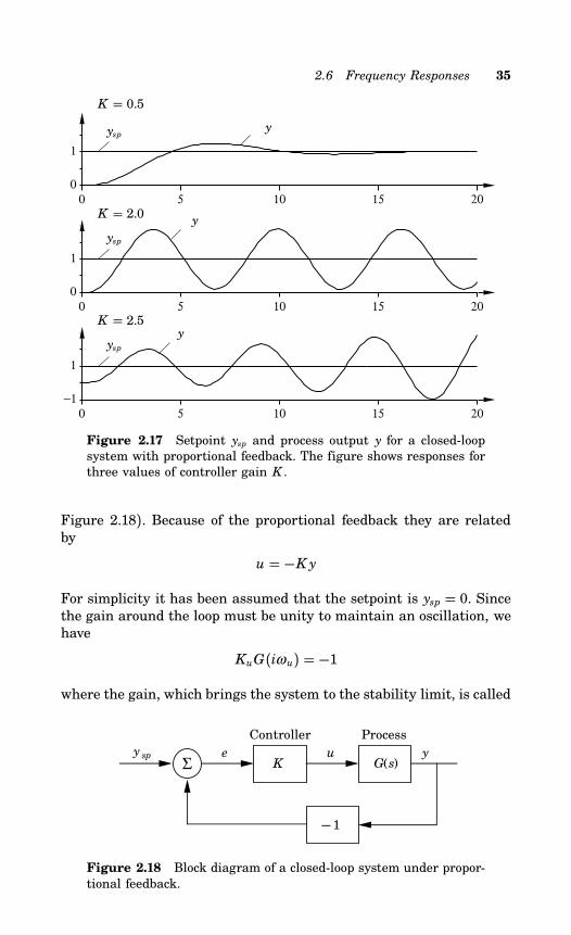
Ziegler and Nichols have provided a method for determining the ulti-mate point on the Nyquist curve experimentally. The method is basedon the observation that many systems can be made unstable underproportional feedback by choosing sufficiently high gain in the propor-tional feedback (see Figure 2.17). Assume that the gain is adjusted sothat the process is at the stability boundary. The control signal andthe process output are then sinusoids with a phase shift of −180 (see
2.6 Frequency Responses 35
0 5 10 15 200
1
0 5 10 15 200
1
0 5 10 15 20−1
1
K = 0.5
K = 2.0
K = 2.5
ysp
ysp
ysp
y
y
y
Figure 2.17 Setpoint ysp and process output y for a closed-loopsystem with proportional feedback. The figure shows responses forthree values of controller gain K .
Figure 2.18). Because of the proportional feedback they are relatedby
u = −K y
For simplicity it has been assumed that the setpoint is ysp = 0. Sincethe gain around the loop must be unity to maintain an oscillation, wehave
KuG(iωu) = −1
where the gain, which brings the system to the stability limit, is called
Σ K
− 1
e u y
ProcessController
G(s) y sp
Figure 2.18 Block diagram of a closed-loop system under propor-tional feedback.
36 Chapter 2 Process Models
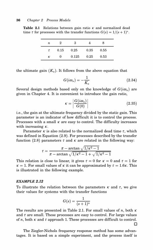
Table 2.1 Relations between gain ratio κ and normalized deadtime τ for processes with the transfer functions G(s) = 1/(s+ 1)n.
n 2 3 4 8
τ 0.15 0.25 0.35 0.55
κ 0 0.125 0.25 0.53
the ultimate gain (Ku). It follows from the above equation that
G(iωu) = − 1Ku
(2.34)
Several design methods based only on the knowledge of G(iωu) aregiven in Chapter 4. It is convenient to introduce the gain ratio,
κ =∣∣∣∣G(iωu)G(0)
∣∣∣∣ (2.35)
i.e., the gain at the ultimate frequency divided by the static gain. Thisparameter is an indicator of how difficult it is to control the process.Processes with a small κ are easy to control. The difficulty increaseswith increasing κ .Parameter κ is also related to the normalized dead time τ , which
was defined in Equation (2.9). For processes described by the transferfunction (2.8) parameters τ and κ are related in the following way:
τ = π − arctan√1/κ 2 − 1
π − arctan√1/κ 2 − 1+
√1/κ 2 − 1
This relation is close to linear, it gives τ = 0 for κ = 0 and τ = 1 forκ = 1. For small values of κ it can be approximated by τ = 1.6κ . Thisis illustrated in the following example.
EXAMPLE 2.12
To illustrate the relation between the parameters κ and τ , we givetheir values for systems with the transfer functions
G(s) = 1(s+ 1)n
The results are presented in Table 2.1. For small values of n, both κand τ are small. These processes are easy to control. For large valuesof n, both κ and τ approach 1. These processes are difficult to control.
The Ziegler-Nichols frequency response method has some advan-tages. It is based on a simple experiment, and the process itself is
2.6 Frequency Responses 37
Σ
− 1
e u y
ProcessRelay
G(s)y sp
Figure 2.19 Block diagram of a process under relay feedback.
used to find the ultimate frequency. It is, however, difficult to auto-mate this experiment or perform it in such a way that the amplitudeof the oscillation is kept under control. Operating the process near in-stability is also dangerous and may need management authorizationin an industrial plant. It is difficult to use this method for automatictuning. An alternative method for automatic determination of specificpoints on the Nyquist curve is suggested below.
Relay Feedback
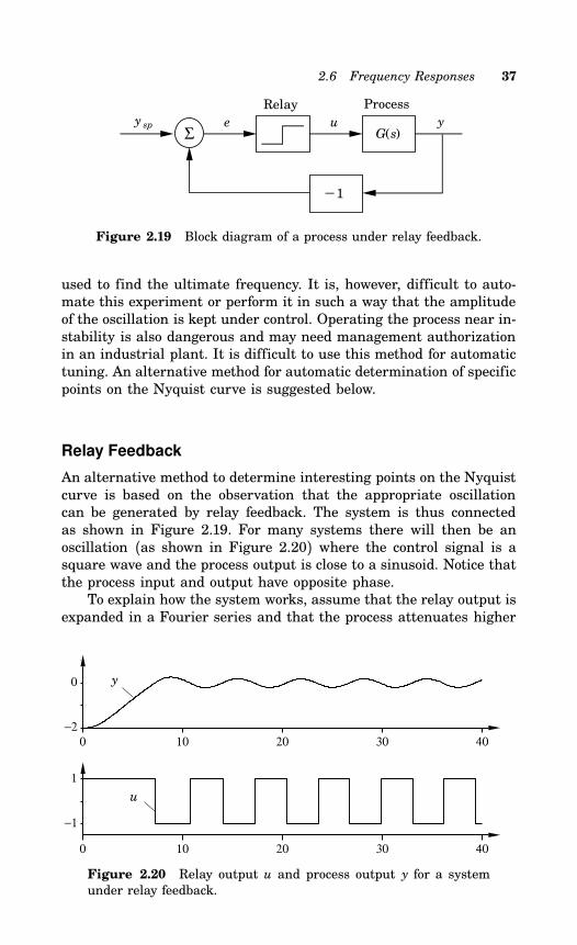
An alternative method to determine interesting points on the Nyquistcurve is based on the observation that the appropriate oscillationcan be generated by relay feedback. The system is thus connectedas shown in Figure 2.19. For many systems there will then be anoscillation (as shown in Figure 2.20) where the control signal is asquare wave and the process output is close to a sinusoid. Notice thatthe process input and output have opposite phase.To explain how the system works, assume that the relay output is
expanded in a Fourier series and that the process attenuates higher
0 10 20 30 40−2
0
0 10 20 30 40
−1
1
y
u
Figure 2.20 Relay output u and process output y for a systemunder relay feedback.
38 Chapter 2 Process Models
harmonics effectively. It is then sufficient to consider the first har-monic component of the input only. The input and the output thenhave opposite phase, which means that the frequency of the oscilla-tion is the ultimate frequency. If d is the relay amplitude, the firstharmonic of the square wave has amplitude 4d/π . Let a be the am-plitude of the oscillation in the process output. Then,
G(iωu) = −π a
4d(2.36)
Notice that the relay experiment is easily automated. Since the am-plitude of the oscillation is proportional to the relay output, it is easyto control it by adjusting the relay output. Also notice in Figure 2.20that a stable oscillation is established very quickly. The amplitudeand the period can be determined after about 20 s only, in spite ofthe fact that the system is started so far from the equilibrium that ittakes about 8 s to reach the correct level. The average residence timeof the system is 12 s, which means that it would take about 40 s fora step response to reach steady state.
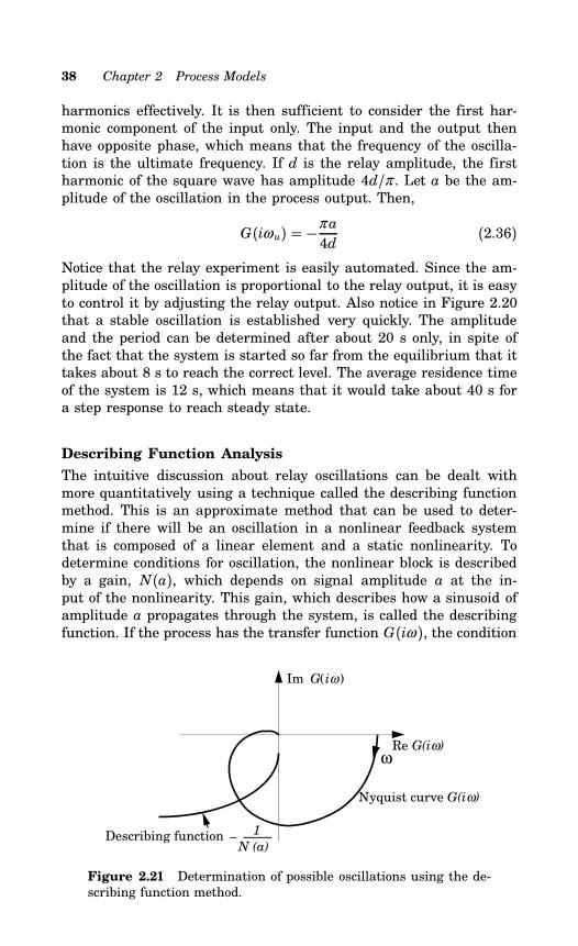
Describing Function Analysis
The intuitive discussion about relay oscillations can be dealt withmore quantitatively using a technique called the describing functionmethod. This is an approximate method that can be used to deter-mine if there will be an oscillation in a nonlinear feedback systemthat is composed of a linear element and a static nonlinearity. Todetermine conditions for oscillation, the nonlinear block is describedby a gain, N(a), which depends on signal amplitude a at the in-put of the nonlinearity. This gain, which describes how a sinusoid ofamplitude a propagates through the system, is called the describingfunction. If the process has the transfer function G(iω ), the condition
Describing function 1
N (a)
ω
−
Re G(iω)
Nyquist curve G(iω)
G(iω) Im
Figure 2.21 Determination of possible oscillations using the de-scribing function method.
2.6 Frequency Responses 39
for oscillation is simply given by
N(a)G(iω ) = −1 (2.37)This equation is obtained by requiring that a sine wave with frequencyω should propagate around the feedback loop with the same ampli-tude and phase. The equation gives two equations for determining aand ω , since N and G may be complex numbers. The equation can besolved graphically by plotting −1/N(a) in the Nyquist diagram (as inFigure 2.21) together with the Nyquist curve G(iω ) of the linear sys-tem. An oscillation may occur if there is an intersection between thetwo curves. The amplitude and the frequency of the oscillation are thesame as the parameters of the two curves at the intersection point.Therefore, measuring the amplitude and the period of the oscillation,the position of one point of the Nyquist curve can be determined.The describing function, N(a), for a relay is given by
N(a) = 4dπ a
(2.38)
Since this function is real, an oscillation may occur if the Nyquistcurve intersects the negative real axis. This explains why the exper-iment with relay feedback gives the point where the Nyquist curveintersects the negative real axis.
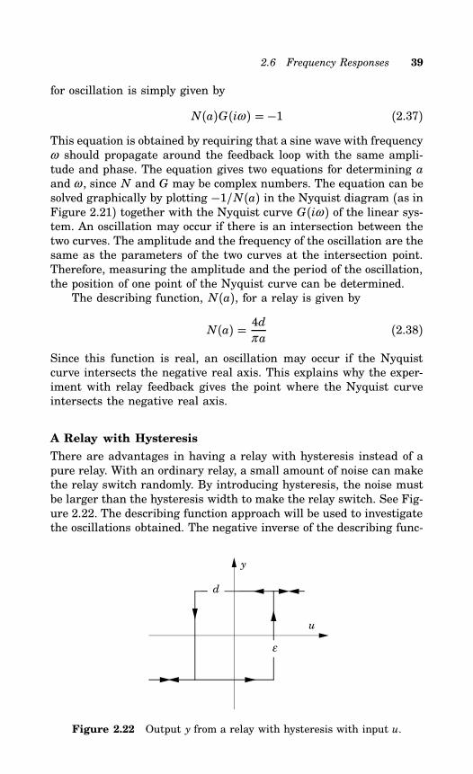
A Relay with Hysteresis
There are advantages in having a relay with hysteresis instead of apure relay. With an ordinary relay, a small amount of noise can makethe relay switch randomly. By introducing hysteresis, the noise mustbe larger than the hysteresis width to make the relay switch. See Fig-ure 2.22. The describing function approach will be used to investigatethe oscillations obtained. The negative inverse of the describing func-
y
d
u
ε
Figure 2.22 Output y from a relay with hysteresis with input u.
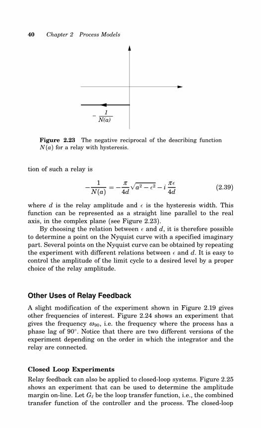
40 Chapter 2 Process Models
−1
N(a)
Figure 2.23 The negative reciprocal of the describing functionN(a) for a relay with hysteresis.
tion of such a relay is
− 1N(a) = −
π
4d
√a2 − ε
2 − i π ε
4d(2.39)
where d is the relay amplitude and ε is the hysteresis width. Thisfunction can be represented as a straight line parallel to the realaxis, in the complex plane (see Figure 2.23).By choosing the relation between ε and d, it is therefore possible
to determine a point on the Nyquist curve with a specified imaginarypart. Several points on the Nyquist curve can be obtained by repeatingthe experiment with different relations between ε and d. It is easy tocontrol the amplitude of the limit cycle to a desired level by a properchoice of the relay amplitude.
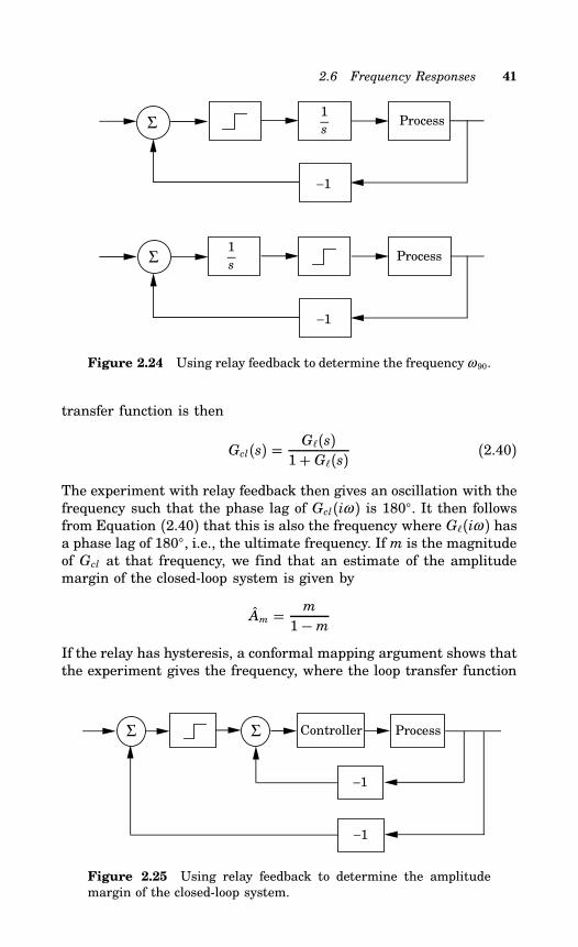
Other Uses of Relay Feedback
A slight modification of the experiment shown in Figure 2.19 givesother frequencies of interest. Figure 2.24 shows an experiment thatgives the frequency ω 90, i.e. the frequency where the process has aphase lag of 90. Notice that there are two different versions of theexperiment depending on the order in which the integrator and therelay are connected.
Closed Loop Experiments
Relay feedback can also be applied to closed-loop systems. Figure 2.25shows an experiment that can be used to determine the amplitudemargin on-line. Let G be the loop transfer function, i.e., the combinedtransfer function of the controller and the process. The closed-loop
2.6 Frequency Responses 41
ProcessΣ1
s
−1
ProcessΣ1
s
−1
Figure 2.24 Using relay feedback to determine the frequencyω 90.
transfer function is then
Gcl(s) = G(s)1+ G(s) (2.40)
The experiment with relay feedback then gives an oscillation with thefrequency such that the phase lag of Gcl(iω ) is 180. It then followsfrom Equation (2.40) that this is also the frequency where G(iω ) hasa phase lag of 180, i.e., the ultimate frequency. If m is the magnitudeof Gcl at that frequency, we find that an estimate of the amplitudemargin of the closed-loop system is given by
Am = m
1−mIf the relay has hysteresis, a conformal mapping argument shows thatthe experiment gives the frequency, where the loop transfer function
ProcessΣ
Σ Controller
−1
−1
Figure 2.25 Using relay feedback to determine the amplitudemargin of the closed-loop system.
42 Chapter 2 Process Models
−1
B
A
Im G l iω( )
Re G iω( )
G iω( )
l
l
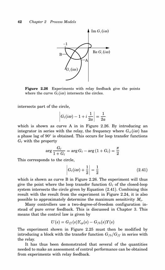
Figure 2.26 Experiments with relay feedback give the pointswhere the curve G(iω ) intersects the circles.
intersects part of the circle,∣∣∣∣G(iω ) − 1+ i 12a∣∣∣∣ = 12a
which is shown as curve A in in Figure 2.26. By introducing anintegrator in series with the relay, the frequency where Gcl(iω ) hasa phase lag of 90 is obtained. This occurs for loop transfer functionsG with the property
argG1+ G = argG − arg (1+ G) =
π
2
This corresponds to the circle,∣∣∣∣G(iω ) + 12∣∣∣∣ = 12 (2.41)
which is shown as curve B in Figure 2.26. The experiment will thusgive the point where the loop transfer function G of the closed-loopsystem intersects the circle given by Equation (2.41). Combining thisresult with the result from the experiment in Figure 2.24, it is alsopossible to approximately determine the maximum sensitivity Ms.Many controllers use a two-degree-of-freedom configuration in-
stead of pure error feedback. This is discussed in Chapter 3. Thismeans that the control law is given by
U (s) = Gf f (s)Ysp(s) − Gfb(s)Y(s)The experiment shown in Figure 2.25 must then be modified byintroducing a block with the transfer function Gfb/Gf f in series withthe relay.It has thus been demonstrated that several of the quantities
needed to make an assessment of control performance can be obtainedfrom experiments with relay feedback.
2.7 Parameter Estimation 43
2.7 Parameter Estimation
A mathematical model of the process can also be obtained by fittingthe parameters of a model to experimental data. For example, a modelof the type given by Equation 2.8 can be obtained by adjusting theparameters so that they match observed input/output data. The ad-vantage of such an approach is that any type of input/output data canbe used. However, parameter estimation requires more computationsthan the methods discussed previously.
Parametric Models
Since the calculations will typically be made using a digital computer,the input/output data will typically be sampled. It is then convenientto operate with a discrete time model based on signals that are sam-pled periodically. Moreover, if the experimental data is also computer-generated, it is reasonable to assume that the input to the process isconstant between the sampling instants. Let the sampling period beh. Assume that time delay L is less than h. The model (2.8) can thenbe described as
y(kh) = ay(kh− h) + b1u(kh − h) + b2u(kh − 2h) (2.42)where
a = e−h/T
b1 = K(1− e−(h−L)/T
)b2 = K e−h/T
(eL/T − 1
)For arbitrary time delays L, the model becomes instead
y(kh) = ay(kh− h) + b1u(kh − nh) + b2u(kh − nh− h) (2.43)where parameters a, b1, and b2 are given as above with n = L div hand τ = Lmod h replacing L. The model can be given a convenientrepresentation by introducing a shift operator q, defined by
qy(kh) = y(kh+ h)The model (2.43) can then be written as
qn(q− a)y(kh) = (b1q+ b2)u(kh)If the complex variable z (similar to the Laplace transform variable s)is introduced, the process can also be described by the pulse transferfunction:
H(z) = b1z+ b2zn(z− a) (2.44)
44 Chapter 2 Process Models
Notice that the transfer function is a ratio of two polynomials even ifthe corresponding physical process has time delays.The discussion can be extended to systems of higher order, and
the result is then an input/output relation of the form:
y(kh) + a1y(kh− h) + ⋅ ⋅ ⋅+ any(kh− nh)= b1u(kh − h) + ⋅ ⋅ ⋅+ bnu(kh − nh)
This equation can be written compactly as
A(q)y(kh) = B(q)u(kh) (2.45)
where A(q) and B(q) are polynomials:
A(q) = qn + a1qn−1 + ⋅ ⋅ ⋅+ anB(q) = b1qn−1 + b2qn−2 + ⋅ ⋅ ⋅+ bn
The corresponding transfer function is then
H(z) = B(z)A(z) =
b1zn−1 + b2zn−2 + ⋅ ⋅ ⋅+ bnzn + a1zn−1 + ⋅ ⋅ ⋅+ an
Parameter Estimation
There are many ways to estimate the parameters of the discrete timemodel (Equation 2.45). A simple method is as follows. Assume that asequence of input/output pairs (u(kh), y(kh), k = 1, 2, . . . ,N) havebeen observed. The parameters can then be determined in such away that Equation (2.45) fits the data as well as possible in the leastsquares sense. The sum of the squares of the errors is
V (θ) =N∑
k=n+1e2(kh) (2.46)
where
e(kh+ nh) = A(q)y(kh) − B(q)u(kh), k = 1, ⋅ ⋅ ⋅ ,N − n
Notice that the error is linear in parameters ai and bi of the modeland that the sum of squares of the errors is a quadratic function.This means that the minimum of the loss function can be computedanalytically. Rather than showing the solution to the optimizationproblem, a convenient way of computing the parameters recursivelyis presented below.
2.7 Parameter Estimation 45
Recursive Computations
In a tuning experiment, a new input/output pair is normally obtainedin each sampling. It is then convenient to compute the parameterestimates recursively. All parameters are grouped together in thevector:
θ = (a1 a2 . . .an b1 b2 . . . bn)T
Introduce the regression vector defined by
ϕ k−1 = (−y(kh− h) . . .− y(kh− nh)u(kh − h) . . .u(kh − nh))T
The estimate can then be calculated recursively by
ek = y(kh) −ϕTk−1θ k−1 (2.47A)
Pk = Pk−1 − Pk−1ϕ k−1ϕTk−1Pk−1
1+ϕTk−1Pk−1ϕ k−1(2.47B)
θ k = θ k−1 + Pkϕ k−1ek (2.47C)These equations have good physical interpretations. The new estimateθ k is obtained by adding a correction term Pϕ e to the old estimateθ k−1. The correction term is a product of three quantities: P, ϕ , ande. The error e is the difference between the last measurement y(kh)and the prediction ϕTθ of this measurement based on old estimates.Regression vector ϕ can be interpreted as the gradient of the errorwith respect to the parameters. This vector tells how the scalar erroris distributed to give corrections in all parameters.Equation (2.47B) may be interpreted as follows. Matrix Pk is
proportional to the covariance matrix of the estimates; the last termin Equation (2.47B) is the reduction in uncertainty due to the lastmeasurement.The equations have to be initialized. The initial value of parame-
ter vector θ can be chosen as the best initial guesses of the parame-ters. The initial value of matrix P is typically chosen as the identitymatrix multiplied by a large number.
Computer Code
Recursive least squares estimation is an essential part of manyschemes for automatic tuning. The following is a computer code thatimplements the algorithm.
The recursive least squares algorithme=yfor i=1 to 2*n do e=e-ϕ[i]*θ[i]
Compute estimator gainfor i=1 to 2*n do
46 Chapter 2 Process Models
begins=0d=1for j=1 to 2*n do
begins=s+P[i,j]*ϕ[j]d=d+s*ϕ[j]
endr[i]=s
endUpdate estimates
for i=1 to 2*n do θ[i]=θ[i]+r[i]*e/dUpdate P matrix
for i=1 to 2*n dobeginfor j=i to 2*n do P[i,j]=P[i,j]-r[i]*r[j]/dfor j=i+1 to 2*n do P[j,i]=P[i,j]end
Update ϕ-vectorfor i=1 to 2*n-1 do ϕ[2*n-i+1]=ϕ[2*n-i]ϕ[1]=-yϕ[n+1]=u
The code description is given in “pidgin” Pascal, and it is assumedthat the variables have been properly declared. There are many re-finements to the algorithm; for instance, its numerical properties canbe improved by using a so-called square root algorithm. It is also com-mon practice to bandpass filter the signals before introducing theminto the algorithm to get rid of static levels and high frequency distur-bances. There are also many variations of the algorithm to discountpast data. The code gives an indication of the type of algorithms thatare used in recursive parameter estimation.
2.8 Disturbance Models
So far, we have only discussed modeling of process dynamics. Dis-turbances is another important side of the control problem. In fact,without disturbances and process uncertainty there would be no needfor feedback. There is a special branch of control, stochastic controltheory, that deals explicitly with disturbances. This has had littleimpact on tuning and design of PID controllers. For PID control, dis-turbances have mostly been considered indirectly, e.g., by introducingintegral action. As our ambitions increase and we strive for controlsystems with improved performances it will be useful to consider dis-turbances explicitly. In this section, therefore, we will present somemodels that can be used for this purpose.
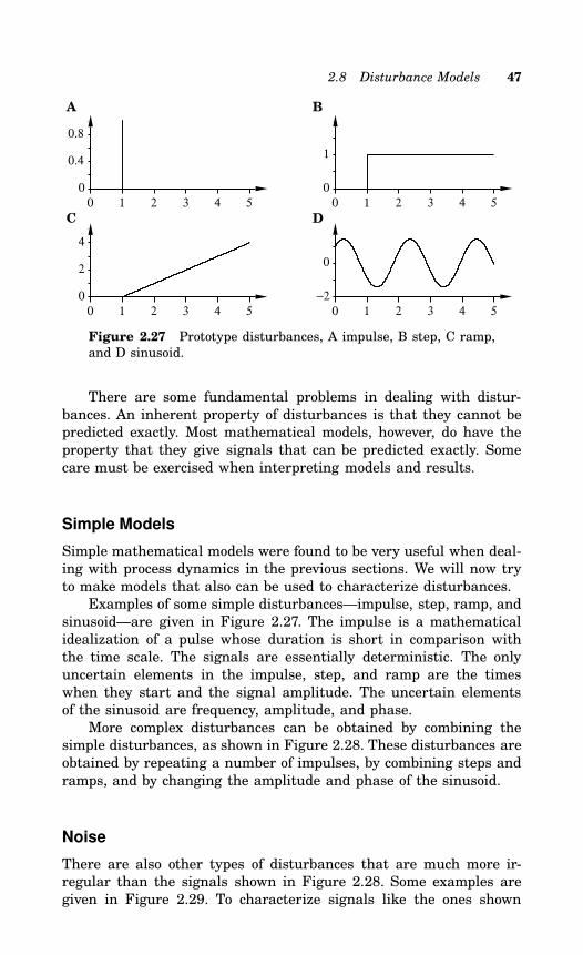
2.8 Disturbance Models 47
0 1 2 3 4 50
0.4
0.8
0 1 2 3 4 50
2
4
0 1 2 3 4 50
1
0 1 2 3 4 5−2
0
A
C
B
D
Figure 2.27 Prototype disturbances, A impulse, B step, C ramp,and D sinusoid.
There are some fundamental problems in dealing with distur-bances. An inherent property of disturbances is that they cannot bepredicted exactly. Most mathematical models, however, do have theproperty that they give signals that can be predicted exactly. Somecare must be exercised when interpreting models and results.
Simple Models
Simple mathematical models were found to be very useful when deal-ing with process dynamics in the previous sections. We will now tryto make models that also can be used to characterize disturbances.Examples of some simple disturbances—impulse, step, ramp, and
sinusoid—are given in Figure 2.27. The impulse is a mathematicalidealization of a pulse whose duration is short in comparison withthe time scale. The signals are essentially deterministic. The onlyuncertain elements in the impulse, step, and ramp are the timeswhen they start and the signal amplitude. The uncertain elementsof the sinusoid are frequency, amplitude, and phase.More complex disturbances can be obtained by combining the
simple disturbances, as shown in Figure 2.28. These disturbances areobtained by repeating a number of impulses, by combining steps andramps, and by changing the amplitude and phase of the sinusoid.
Noise
There are also other types of disturbances that are much more ir-regular than the signals shown in Figure 2.28. Some examples aregiven in Figure 2.29. To characterize signals like the ones shown
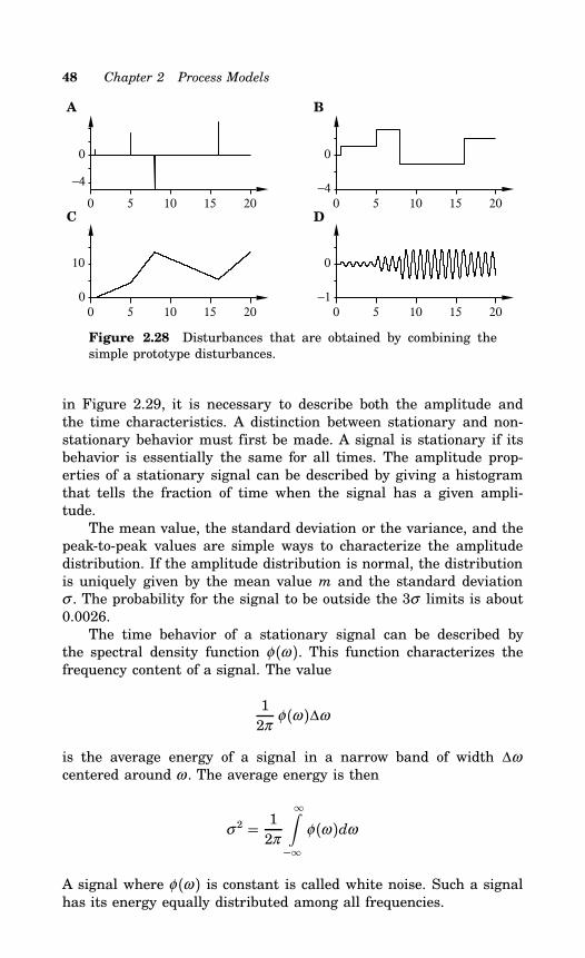
48 Chapter 2 Process Models
0 5 10 15 20
−4
0
0 5 10 15 200
10
0 5 10 15 20−4
0
0 5 10 15 20−1
0
A
C
B
D
Figure 2.28 Disturbances that are obtained by combining thesimple prototype disturbances.
in Figure 2.29, it is necessary to describe both the amplitude andthe time characteristics. A distinction between stationary and non-stationary behavior must first be made. A signal is stationary if itsbehavior is essentially the same for all times. The amplitude prop-erties of a stationary signal can be described by giving a histogramthat tells the fraction of time when the signal has a given ampli-tude.The mean value, the standard deviation or the variance, and the
peak-to-peak values are simple ways to characterize the amplitudedistribution. If the amplitude distribution is normal, the distributionis uniquely given by the mean value m and the standard deviationσ . The probability for the signal to be outside the 3σ limits is about0.0026.The time behavior of a stationary signal can be described by
the spectral density function φ(ω ). This function characterizes thefrequency content of a signal. The value
12π
φ(ω )∆ω
is the average energy of a signal in a narrow band of width ∆ωcentered around ω . The average energy is then
σ 2 = 12π
∞∫−∞
φ(ω )dω
A signal where φ(ω ) is constant is called white noise. Such a signalhas its energy equally distributed among all frequencies.
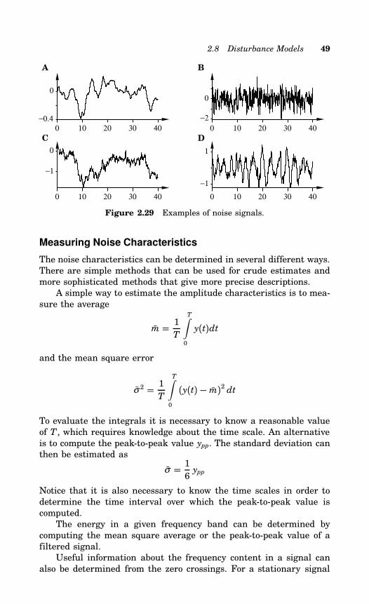
2.8 Disturbance Models 49
0 10 20 30 40−0.4
0
0 10 20 30 40
−1
0
0 10 20 30 40
−2
0
0 10 20 30 40
−1
1
A
C
B
D
Figure 2.29 Examples of noise signals.
Measuring Noise Characteristics
The noise characteristics can be determined in several different ways.There are simple methods that can be used for crude estimates andmore sophisticated methods that give more precise descriptions.A simple way to estimate the amplitude characteristics is to mea-
sure the average
m = 1T
T∫0
y(t)dt
and the mean square error
σ 2 = 1T
T∫0
(y(t) − m)2 dt
To evaluate the integrals it is necessary to know a reasonable valueof T , which requires knowledge about the time scale. An alternativeis to compute the peak-to-peak value ypp. The standard deviation canthen be estimated as
σ = 16ypp
Notice that it is also necessary to know the time scales in order todetermine the time interval over which the peak-to-peak value iscomputed.The energy in a given frequency band can be determined by
computing the mean square average or the peak-to-peak value of afiltered signal.Useful information about the frequency content in a signal can
also be determined from the zero crossings. For a stationary signal
50 Chapter 2 Process Models
the average number of zero crossings per second can be determinedfrom
N = 1π
∞∫−∞
ω 2φ(ω )dω∞∫−∞
φ(ω )dω
1/2
where φ(ω ) is the spectral density. Notice that this formula has simi-larities with the formula for determining the average residence time,Equation (2.24).For a spectral density that is uniform over the interval (ω 1,ω 2),
we get
N = 1π
(ω 32 −ω 313(ω 2 −ω 1)
)1/2= 1
π
(ω 21 +ω 1ω 2 +ω 223
)1/2For an ideal low-pass filter we have ω 1 = 0 and ω 2 = ω b, where ω bis the band width. In this case we get
N = ω b
π√3= 2π fb
π√3 1.16 fb
The average rate of zero crossings per second is thus approximatelyequal to the bandwidth measured in Hz. Measurement of zero cross-ings can easily be combined with computation of the peak-to-peakvalue. More accurate determination of the spectral characteristics canbe done by using a spectral analyzer or by recording a data set andcomputing the spectrum numerically.
Representation of Disturbances
It is often very convenient to consider signals as generated from adynamic system with simple inputs as shown in Figure 2.30. Forexample, the signals shown in Figure 2.27 can be represented bysending an impulse through a dynamic system. The transfer functionof the systems for the different signals are
Impulse G(s) = 1Step G(s) = 1
s
Ramp G(s) = 1s2
Sinusoid G(s) = ω 2
s2 +ω 2
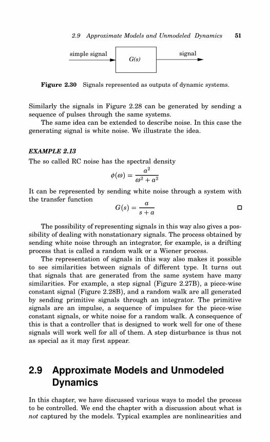
2.9 Approximate Models and Unmodeled Dynamics 51
signalG(s)
simple signal
Figure 2.30 Signals represented as outputs of dynamic systems.
Similarly the signals in Figure 2.28 can be generated by sending asequence of pulses through the same systems.The same idea can be extended to describe noise. In this case the
generating signal is white noise. We illustrate the idea.
EXAMPLE 2.13
The so called RC noise has the spectral density
φ(ω ) = a2
ω 2 + a2It can be represented by sending white noise through a system withthe transfer function
G(s) = a
s+ aThe possibility of representing signals in this way also gives a pos-
sibility of dealing with nonstationary signals. The process obtained bysending white noise through an integrator, for example, is a driftingprocess that is called a random walk or a Wiener process.The representation of signals in this way also makes it possible
to see similarities between signals of different type. It turns outthat signals that are generated from the same system have manysimilarities. For example, a step signal (Figure 2.27B), a piece-wiseconstant signal (Figure 2.28B), and a random walk are all generatedby sending primitive signals through an integrator. The primitivesignals are an impulse, a sequence of impulses for the piece-wiseconstant signals, or white noise for a random walk. A consequence ofthis is that a controller that is designed to work well for one of thesesignals will work well for all of them. A step disturbance is thus notas special as it may first appear.
2.9 Approximate Models and Unmodeled
Dynamics
In this chapter, we have discussed various ways to model the processto be controlled. We end the chapter with a discussion about what isnot captured by the models. Typical examples are nonlinearities and
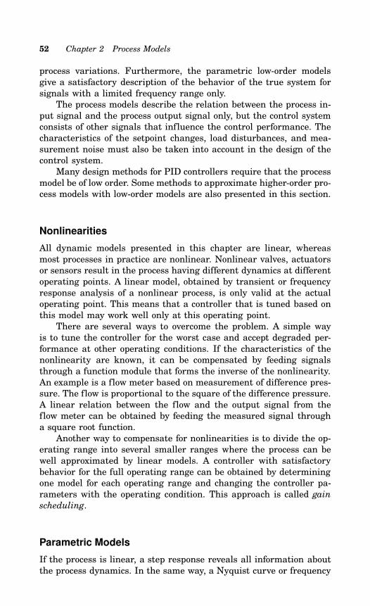
52 Chapter 2 Process Models
process variations. Furthermore, the parametric low-order modelsgive a satisfactory description of the behavior of the true system forsignals with a limited frequency range only.The process models describe the relation between the process in-
put signal and the process output signal only, but the control systemconsists of other signals that influence the control performance. Thecharacteristics of the setpoint changes, load disturbances, and mea-surement noise must also be taken into account in the design of thecontrol system.Many design methods for PID controllers require that the process
model be of low order. Some methods to approximate higher-order pro-cess models with low-order models are also presented in this section.
Nonlinearities
All dynamic models presented in this chapter are linear, whereasmost processes in practice are nonlinear. Nonlinear valves, actuatorsor sensors result in the process having different dynamics at differentoperating points. A linear model, obtained by transient or frequencyresponse analysis of a nonlinear process, is only valid at the actualoperating point. This means that a controller that is tuned based onthis model may work well only at this operating point.There are several ways to overcome the problem. A simple way
is to tune the controller for the worst case and accept degraded per-formance at other operating conditions. If the characteristics of thenonlinearity are known, it can be compensated by feeding signalsthrough a function module that forms the inverse of the nonlinearity.An example is a flow meter based on measurement of difference pres-sure. The flow is proportional to the square of the difference pressure.A linear relation between the flow and the output signal from theflow meter can be obtained by feeding the measured signal througha square root function.Another way to compensate for nonlinearities is to divide the op-
erating range into several smaller ranges where the process can bewell approximated by linear models. A controller with satisfactorybehavior for the full operating range can be obtained by determiningone model for each operating range and changing the controller pa-rameters with the operating condition. This approach is called gainscheduling.
Parametric Models
If the process is linear, a step response reveals all information aboutthe process dynamics. In the same way, a Nyquist curve or frequency
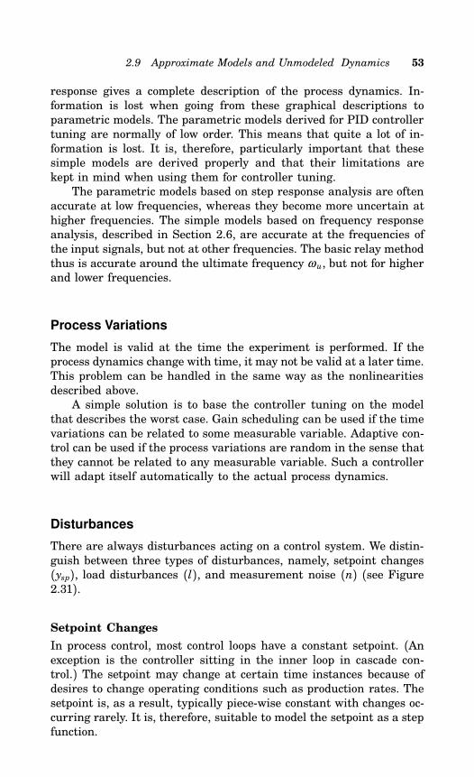
2.9 Approximate Models and Unmodeled Dynamics 53
response gives a complete description of the process dynamics. In-formation is lost when going from these graphical descriptions toparametric models. The parametric models derived for PID controllertuning are normally of low order. This means that quite a lot of in-formation is lost. It is, therefore, particularly important that thesesimple models are derived properly and that their limitations arekept in mind when using them for controller tuning.The parametric models based on step response analysis are often
accurate at low frequencies, whereas they become more uncertain athigher frequencies. The simple models based on frequency responseanalysis, described in Section 2.6, are accurate at the frequencies ofthe input signals, but not at other frequencies. The basic relay methodthus is accurate around the ultimate frequency ωu, but not for higherand lower frequencies.
Process Variations
The model is valid at the time the experiment is performed. If theprocess dynamics change with time, it may not be valid at a later time.This problem can be handled in the same way as the nonlinearitiesdescribed above.A simple solution is to base the controller tuning on the model
that describes the worst case. Gain scheduling can be used if the timevariations can be related to some measurable variable. Adaptive con-trol can be used if the process variations are random in the sense thatthey cannot be related to any measurable variable. Such a controllerwill adapt itself automatically to the actual process dynamics.
Disturbances
There are always disturbances acting on a control system. We distin-guish between three types of disturbances, namely, setpoint changes(ysp), load disturbances (l), and measurement noise (n) (see Figure2.31).
Setpoint Changes
In process control, most control loops have a constant setpoint. (Anexception is the controller sitting in the inner loop in cascade con-trol.) The setpoint may change at certain time instances because ofdesires to change operating conditions such as production rates. Thesetpoint is, as a result, typically piece-wise constant with changes oc-curring rarely. It is, therefore, suitable to model the setpoint as a stepfunction.
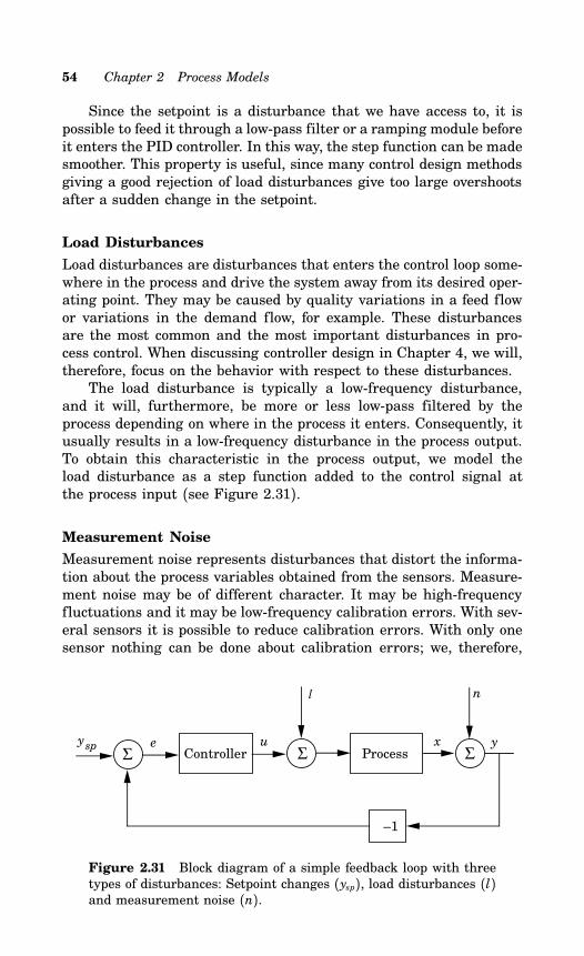
54 Chapter 2 Process Models
Since the setpoint is a disturbance that we have access to, it ispossible to feed it through a low-pass filter or a ramping module beforeit enters the PID controller. In this way, the step function can be madesmoother. This property is useful, since many control design methodsgiving a good rejection of load disturbances give too large overshootsafter a sudden change in the setpoint.
Load Disturbances
Load disturbances are disturbances that enters the control loop some-where in the process and drive the system away from its desired oper-ating point. They may be caused by quality variations in a feed flowor variations in the demand flow, for example. These disturbancesare the most common and the most important disturbances in pro-cess control. When discussing controller design in Chapter 4, we will,therefore, focus on the behavior with respect to these disturbances.The load disturbance is typically a low-frequency disturbance,
and it will, furthermore, be more or less low-pass filtered by theprocess depending on where in the process it enters. Consequently, itusually results in a low-frequency disturbance in the process output.To obtain this characteristic in the process output, we model theload disturbance as a step function added to the control signal atthe process input (see Figure 2.31).
Measurement Noise
Measurement noise represents disturbances that distort the informa-tion about the process variables obtained from the sensors. Measure-ment noise may be of different character. It may be high-frequencyfluctuations and it may be low-frequency calibration errors. With sev-eral sensors it is possible to reduce calibration errors. With only onesensor nothing can be done about calibration errors; we, therefore,
ysp uController ProcessΣΣ
eΣ
x
l
–1
y
n
Figure 2.31 Block diagram of a simple feedback loop with threetypes of disturbances: Setpoint changes (ysp), load disturbances (l)and measurement noise (n).
2.9 Approximate Models and Unmodeled Dynamics 55
will model measurement noise as a high-frequency signal added tothe process output.Since measurement noise does not contain any information about
the status of the process, it should be filtered out. Furthermore, high-frequency components in the measurement signal might be amplifiedby the controller and cause wear on the actuator. Filtering does intro-duce additional dynamics. It is therefore important to take the filterdynamics into account in the controlling design. We will model themeasurement noise as an impulse function.
Approximating Complex Models
In modeling it is often convenient to split a system into interconnectedsubsystems. An example could be to divide a system into actuator, pro-cess, and sensor. Another example occurs when general control loopsare cascaded. We may be interested then in obtaining a simplified de-scription of the closed loop. Even if the model for each part is simple,the complete model may then be quite complex. Since many of thedesign methods for PID controllers are based on simple models, weneed a procedure to simplify a complex model. Some ways to makesuch approximations are discussed below.To perform the approximations it is necessary to determine the
frequency range where the approximation should be valid. We do thissimply by saying that the models should describe the system wellaround the frequency ω 0. This frequency should be approximatelythe same as the frequency of the dominant closed-loop poles of thedesired system or the desired bandwidth of the closed-loop system.(The notion of dominant poles is discussed in Chapter 4.) Havingrestricted the modeling to a rather narrow frequency range, low-ordermodels can now be determined by fitting them to experimental data,as described previously in this section.Another possibility is to start with a complex model of the form
Gp(s) = K 1+ b1s+ b2s2 + ⋅ ⋅ ⋅+ bnsn
1+ a1s+ a2s2 + ⋅ ⋅ ⋅+ ansn e−sL
and approximate it. The approximation is done in the following way.Poles and zeros that are much slower than ω 0 are approximated byintegrators, poles, and zeros of the same order as ω 0 are retained,and poles and zeros that are much faster than ω 0 are neglected orapproximated by a small time lag. A dead time such that ω 0L ≪ 1is neglected or approximated by a time constant. The approximationof fast poles and zeros by a first order system is illustrated by anexample.
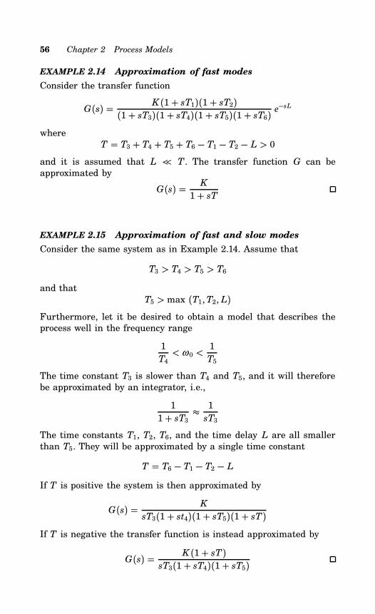
56 Chapter 2 Process Models
EXAMPLE 2.14 Approximation of fast modes
Consider the transfer function
G(s) = K (1+ sT1)(1+ sT2)(1+ sT3)(1+ sT4)(1+ sT5)(1+ sT6) e
−sL
whereT = T3 + T4 + T5 + T6 − T1 − T2 − L > 0
and it is assumed that L ≪ T . The transfer function G can beapproximated by
G(s) = K
1+ sT
EXAMPLE 2.15 Approximation of fast and slow modes
Consider the same system as in Example 2.14. Assume that
T3 > T4 > T5 > T6and that
T5 > max (T1,T2, L)Furthermore, let it be desired to obtain a model that describes theprocess well in the frequency range
1T4< ω 0 < 1
T5
The time constant T3 is slower than T4 and T5, and it will thereforebe approximated by an integrator, i.e.,
11+ sT3
1sT3
The time constants T1, T2, T6, and the time delay L are all smallerthan T5. They will be approximated by a single time constant
T = T6 − T1 − T2 − LIf T is positive the system is then approximated by
G(s) = K
sT3(1+ st4)(1+ sT5)(1+ sT)If T is negative the transfer function is instead approximated by
G(s) = K (1+ sT)sT3(1+ sT4)(1+ sT5)
2.10 Conclusions 57
Summary
To summarize: When deriving a simple model to be used for PIDcontroller tuning, it is important to ensure that the model describesthe process well for the typical input signals obtained during theprocess operations. The amplitude and frequency distribution of thesignal is of importance. Model accuracy may be poor if the process isnonlinear or time varying. Control quality can be improved by gainscheduling or adaptive control. It is also important to know what kindof disturbances are acting on the system and which limitation theyimpose.
2.10 Conclusions
Modeling is an important aspect of controller tuning. The models weneed should describe how the process reacts to control signals. Theyshould also describe the properties of the disturbances that enter thesystem. Most work on tuning of PID controllers have focused on theprocess dynamics, which is also reflected in the presentation in thischapter.A number of methods for determining the dynamics of a process
have been presented in this chapter. Some are very simple: theyare based on a direct measurement of the step response and simplegraphical constructions. Others are based on the frequency response.It has been shown that very useful information can be generated fromrelay feedback experiments. Such experiments are particularly usefulbecause the process is brought into self-oscillation at the ultimatefrequency, which is of considerable interest for design of controllers.The simple methods are useful in field work when a controller
has to be tuned and few tools are available. The methods are alsouseful to provide understanding as well as being references whenmore complicated methods are assessed. We have also presented morecomplicated methods that require significant computations.Models of different complexity have been presented. Many models
were characterized by a few parameters. Such models are useful formany purposes and are discussed in Chapter 4. When using suchmodels it should be kept in mind that they are approximations.When deriving the models we also introduced two dimension-
free quantities, the normalized dead time τ and the gain ratio κ .These parameters make it possible to make a crude assessment ofthe difficulty of controlling the process. Processes with small valuesare easy to control. The difficulty increases as the values approach 1.Tuning rules based on τ and κ are provided in Chapter 5.
58 Chapter 2 Process Models
2.11 References
Process modeling is a key element in understanding and solving a con-trol problem. Good presentations of modeling are found in standardtextbooks on control, such as (Buckley, 1964), (Smith, 1972), (Se-borg et al., 1989), and (Luyben, 1990). These books have much mate-rial on many different modeling techniques. Similar presentations aregiven in (Gille et al., 1959), (Harriott, 1964), (Oppelt, 1964), (Taka-hashi et al., 1972), (Deshpande and Ash, 1981), (Shinskey, 1988),(Stephanopoulos, 1984), and (Hägglund, 1991). There are also booksthat specialize in modeling for control system design, see (Wellstead,1979), (Nicholson, 1980), (Nicholson, 1981), and (Close and Freder-ick, 1993).In the early work much effort was devoted to characterize dynam-
ics by the step response, which at that time was called the responsecurve. See (Ziegler et al., 1943) and the books (Tucker and Wills,1960) and (Lloyd and Anderson, 1971), which were written by prac-titioners in control companies. A nice overview of step and frequencyresponse methods is given in the paper (Rake, 1980). Additional de-tails are given in (Strejc, 1959) and (Anderssen and White, 1971).Frequency response methods are presented in (Anderssen and White,1970).The relay method is treated in (Åström and Hägglund, 1984),
(Hägglund and Åström, 1991), and (Schei, 1992). The describing func-tion method is well documented in (Atherton, 1975) and (Gelb andVelde, 1968). There are many books on parameter estimation, thebook (Johansson, 1993) is quite accessible. More mathematical de-tails are found in (Ljung, 1987), (Ljung and Söderström, 1983), and(Söderström and Stoica, 1988). Many useful practical aspects on sys-tem identification are given in (Isermann, 1980).
PID Control
3.1 Introduction
The PID controller is by far the most common control algorithm. Mostfeedback loops are controlled by this algorithm or minor variationsof it. It is implemented in many different forms, as a stand-alonecontroller or as a part of a DDC (Direct Digital Control) package ora hierarchical distributed process control system. Many thousandsof instrument and control engineers worldwide are using such con-trollers in their daily work. The PID algorithm can be approachedfrom many different directions. It can be viewed as a device that canbe operated with a few rules of thumb, but it can also be approachedanalytically.This chapter gives an introduction to PID control. The basic al-
gorithm and various representations are presented in detail. A de-scription of the properties of the controller in a closed loop based onintuitive arguments is given. The phenomenon of reset windup, whichoccurs when a controller with integral action is connected to a processwith a saturating actuator, is discussed, including several methods toavoid it.Some important aspects of digital computer implementation of
PID controllers are given: issues such as prefiltering, different digi-tal approximations, noise filtering, and computer code for good imple-mentation. Operational aspects, such as bumpless transfer betweenmanual and automatic mode and between different parameter sets,are also presented. The chapter ends with some aspects on the useand misuse of PID control with examples of systems where PID con-trol works well and where it does not.
59
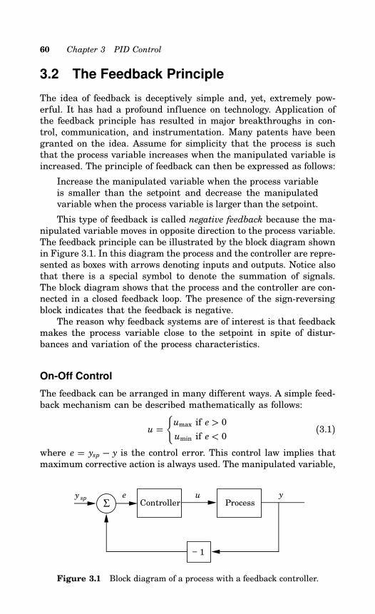
60 Chapter 3 PID Control
3.2 The Feedback Principle
The idea of feedback is deceptively simple and, yet, extremely pow-erful. It has had a profound influence on technology. Application ofthe feedback principle has resulted in major breakthroughs in con-trol, communication, and instrumentation. Many patents have beengranted on the idea. Assume for simplicity that the process is suchthat the process variable increases when the manipulated variable isincreased. The principle of feedback can then be expressed as follows:
Increase the manipulated variable when the process variableis smaller than the setpoint and decrease the manipulatedvariable when the process variable is larger than the setpoint.
This type of feedback is called negative feedback because the ma-nipulated variable moves in opposite direction to the process variable.The feedback principle can be illustrated by the block diagram shownin Figure 3.1. In this diagram the process and the controller are repre-sented as boxes with arrows denoting inputs and outputs. Notice alsothat there is a special symbol to denote the summation of signals.The block diagram shows that the process and the controller are con-nected in a closed feedback loop. The presence of the sign-reversingblock indicates that the feedback is negative.The reason why feedback systems are of interest is that feedback
makes the process variable close to the setpoint in spite of distur-bances and variation of the process characteristics.
On-Off Control
The feedback can be arranged in many different ways. A simple feed-back mechanism can be described mathematically as follows:
u =umax if e > 0umin if e < 0
(3.1)
where e = ysp − y is the control error. This control law implies thatmaximum corrective action is always used. The manipulated variable,
Controller Processe u y
Σ
1−
y sp
Figure 3.1 Block diagram of a process with a feedback controller.
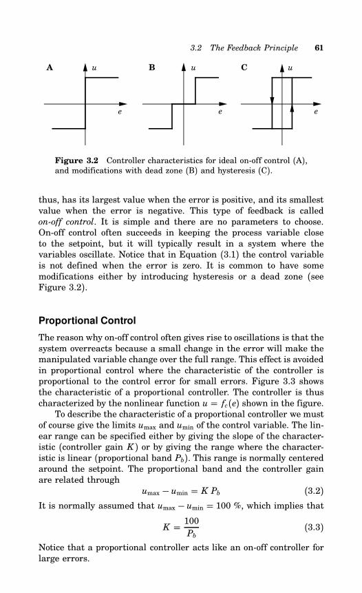
3.2 The Feedback Principle 61
u
e
Cu
e
u
e
BA
Figure 3.2 Controller characteristics for ideal on-off control (A),and modifications with dead zone (B) and hysteresis (C).
thus, has its largest value when the error is positive, and its smallestvalue when the error is negative. This type of feedback is calledon-off control. It is simple and there are no parameters to choose.On-off control often succeeds in keeping the process variable closeto the setpoint, but it will typically result in a system where thevariables oscillate. Notice that in Equation (3.1) the control variableis not defined when the error is zero. It is common to have somemodifications either by introducing hysteresis or a dead zone (seeFigure 3.2).
Proportional Control
The reason why on-off control often gives rise to oscillations is that thesystem overreacts because a small change in the error will make themanipulated variable change over the full range. This effect is avoidedin proportional control where the characteristic of the controller isproportional to the control error for small errors. Figure 3.3 showsthe characteristic of a proportional controller. The controller is thuscharacterized by the nonlinear function u = fc(e) shown in the figure.To describe the characteristic of a proportional controller we must
of course give the limits umax and umin of the control variable. The lin-ear range can be specified either by giving the slope of the character-istic (controller gain K ) or by giving the range where the character-istic is linear (proportional band Pb). This range is normally centeredaround the setpoint. The proportional band and the controller gainare related through
umax − umin = K Pb (3.2)It is normally assumed that umax − umin = 100 %, which implies that
K = 100Pb
(3.3)
Notice that a proportional controller acts like an on-off controller forlarge errors.
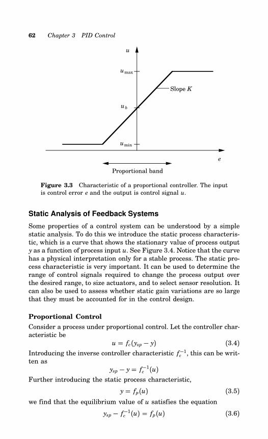
62 Chapter 3 PID Control
u
e
Proportional band
Slope K
umax
ub
umin
Figure 3.3 Characteristic of a proportional controller. The inputis control error e and the output is control signal u.
Static Analysis of Feedback Systems
Some properties of a control system can be understood by a simplestatic analysis. To do this we introduce the static process characteris-tic, which is a curve that shows the stationary value of process outputy as a function of process input u. See Figure 3.4. Notice that the curvehas a physical interpretation only for a stable process. The static pro-cess characteristic is very important. It can be used to determine therange of control signals required to change the process output overthe desired range, to size actuators, and to select sensor resolution. Itcan also be used to assess whether static gain variations are so largethat they must be accounted for in the control design.
Proportional Control
Consider a process under proportional control. Let the controller char-acteristic be
u = fc(ysp − y) (3.4)Introducing the inverse controller characteristic f−1c , this can be writ-ten as
ysp − y= f−1c (u)Further introducing the static process characteristic,
y = fp(u) (3.5)we find that the equilibrium value of u satisfies the equation
ysp − f−1c (u) = fp(u) (3.6)
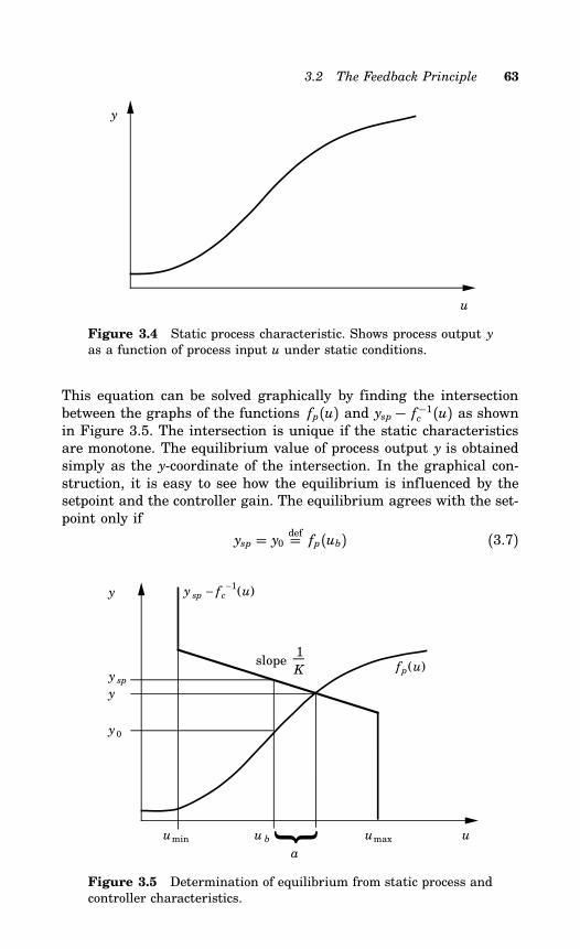
3.2 The Feedback Principle 63
y
u
Figure 3.4 Static process characteristic. Shows process output yas a function of process input u under static conditions.
This equation can be solved graphically by finding the intersectionbetween the graphs of the functions fp(u) and ysp− f−1c (u) as shownin Figure 3.5. The intersection is unique if the static characteristicsare monotone. The equilibrium value of process output y is obtainedsimply as the y-coordinate of the intersection. In the graphical con-struction, it is easy to see how the equilibrium is influenced by thesetpoint and the controller gain. The equilibrium agrees with the set-point only if
ysp = y0 def= fp(ub) (3.7)
yy
a
slope
u u b umaxumin
fp(u)
1
K
y sp − fc−1
(u)
y sp
y
y0
Figure 3.5 Determination of equilibrium from static process andcontroller characteristics.
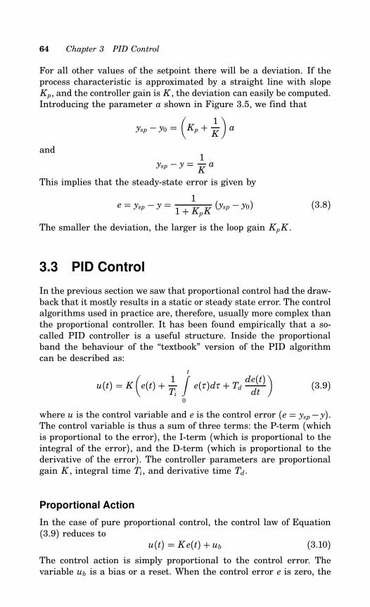
64 Chapter 3 PID Control
For all other values of the setpoint there will be a deviation. If theprocess characteristic is approximated by a straight line with slopeKp, and the controller gain is K , the deviation can easily be computed.Introducing the parameter a shown in Figure 3.5, we find that
ysp − y0 =(Kp + 1
K
)a
and
ysp − y= 1Ka
This implies that the steady-state error is given by
e = ysp − y = 11+ KpK (ysp − y0) (3.8)
The smaller the deviation, the larger is the loop gain KpK .
3.3 PID Control
In the previous section we saw that proportional control had the draw-back that it mostly results in a static or steady state error. The controlalgorithms used in practice are, therefore, usually more complex thanthe proportional controller. It has been found empirically that a so-called PID controller is a useful structure. Inside the proportionalband the behaviour of the “textbook” version of the PID algorithmcan be described as:
u(t) = K(e(t) + 1
Ti
t∫0
e(τ )dτ + Td de(t)dt
)(3.9)
where u is the control variable and e is the control error (e = ysp− y).The control variable is thus a sum of three terms: the P-term (whichis proportional to the error), the I-term (which is proportional to theintegral of the error), and the D-term (which is proportional to thederivative of the error). The controller parameters are proportionalgain K , integral time Ti, and derivative time Td.
Proportional Action
In the case of pure proportional control, the control law of Equation(3.9) reduces to
u(t) = K e(t) + ub (3.10)The control action is simply proportional to the control error. Thevariable ub is a bias or a reset. When the control error e is zero, the
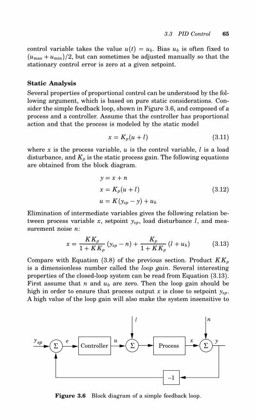
3.3 PID Control 65
control variable takes the value u(t) = ub. Bias ub is often fixed to(umax + umin)/2, but can sometimes be adjusted manually so that thestationary control error is zero at a given setpoint.
Static Analysis
Several properties of proportional control can be understood by the fol-lowing argument, which is based on pure static considerations. Con-sider the simple feedback loop, shown in Figure 3.6, and composed of aprocess and a controller. Assume that the controller has proportionalaction and that the process is modeled by the static model
x = Kp(u + l) (3.11)where x is the process variable, u is the control variable, l is a loaddisturbance, and Kp is the static process gain. The following equationsare obtained from the block diagram.
y= x + nx = Kp(u + l)u = K (ysp − y) + ub
(3.12)
Elimination of intermediate variables gives the following relation be-tween process variable x, setpoint ysp, load disturbance l, and mea-surement noise n:
x = K Kp
1+ K Kp (ysp − n) +Kp
1+ K Kp (l + ub) (3.13)
Compare with Equation (3.8) of the previous section. Product K Kpis a dimensionless number called the loop gain. Several interestingproperties of the closed-loop system can be read from Equation (3.13).First assume that n and ub are zero. Then the loop gain should behigh in order to ensure that process output x is close to setpoint ysp.A high value of the loop gain will also make the system insensitive to
ysp uController ProcessΣΣ
eΣ
x
l
–1
y
n
Figure 3.6 Block diagram of a simple feedback loop.
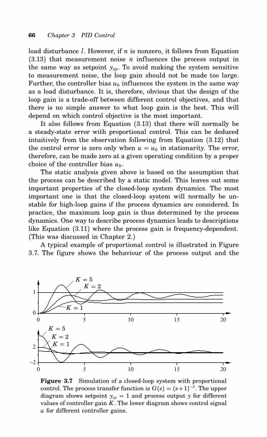
66 Chapter 3 PID Control
load disturbance l. However, if n is nonzero, it follows from Equation(3.13) that measurement noise n influences the process output inthe same way as setpoint ysp. To avoid making the system sensitiveto measurement noise, the loop gain should not be made too large.Further, the controller bias ub influences the system in the same wayas a load disturbance. It is, therefore, obvious that the design of theloop gain is a trade-off between different control objectives, and thatthere is no simple answer to what loop gain is the best. This willdepend on which control objective is the most important.It also follows from Equation (3.13) that there will normally be
a steady-state error with proportional control. This can be deducedintuitively from the observation following from Equation (3.12) thatthe control error is zero only when u = ub in stationarity. The error,therefore, can be made zero at a given operating condition by a properchoice of the controller bias ub.The static analysis given above is based on the assumption that
the process can be described by a static model. This leaves out someimportant properties of the closed-loop system dynamics. The mostimportant one is that the closed-loop system will normally be un-stable for high-loop gains if the process dynamics are considered. Inpractice, the maximum loop gain is thus determined by the processdynamics. One way to describe process dynamics leads to descriptionslike Equation (3.11) where the process gain is frequency-dependent.(This was discussed in Chapter 2.)A typical example of proportional control is illustrated in Figure
3.7. The figure shows the behaviour of the process output and the
0 5 10 15 200
1
0 5 10 15 20−2
2
K = 5K = 2
K = 1
K = 5K = 2K = 1
Figure 3.7 Simulation of a closed-loop system with proportionalcontrol. The process transfer function is G(s) = (s+1)−3. The upperdiagram shows setpoint ysp = 1 and process output y for differentvalues of controller gain K . The lower diagram shows control signalu for different controller gains.
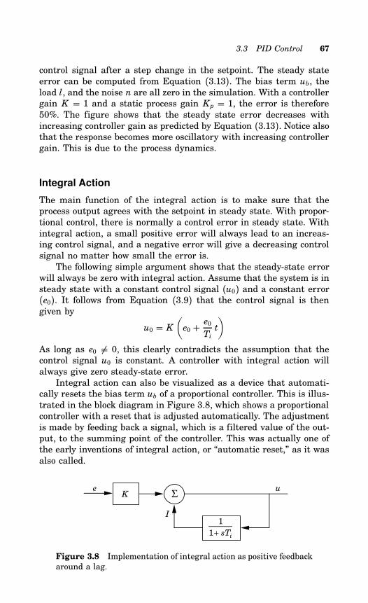
3.3 PID Control 67
control signal after a step change in the setpoint. The steady stateerror can be computed from Equation (3.13). The bias term ub, theload l, and the noise n are all zero in the simulation. With a controllergain K = 1 and a static process gain Kp = 1, the error is therefore50%. The figure shows that the steady state error decreases withincreasing controller gain as predicted by Equation (3.13). Notice alsothat the response becomes more oscillatory with increasing controllergain. This is due to the process dynamics.
Integral Action
The main function of the integral action is to make sure that theprocess output agrees with the setpoint in steady state. With propor-tional control, there is normally a control error in steady state. Withintegral action, a small positive error will always lead to an increas-ing control signal, and a negative error will give a decreasing controlsignal no matter how small the error is.The following simple argument shows that the steady-state error
will always be zero with integral action. Assume that the system is insteady state with a constant control signal (u0) and a constant error(e0). It follows from Equation (3.9) that the control signal is thengiven by
u0 = K(e0 + e0
Tit
)As long as e0 = 0, this clearly contradicts the assumption that thecontrol signal u0 is constant. A controller with integral action willalways give zero steady-state error.Integral action can also be visualized as a device that automati-
cally resets the bias term ub of a proportional controller. This is illus-trated in the block diagram in Figure 3.8, which shows a proportionalcontroller with a reset that is adjusted automatically. The adjustmentis made by feeding back a signal, which is a filtered value of the out-put, to the summing point of the controller. This was actually one ofthe early inventions of integral action, or “automatic reset,” as it wasalso called.
ΣK
I
e u
1
1+ sTi
Figure 3.8 Implementation of integral action as positive feedbackaround a lag.
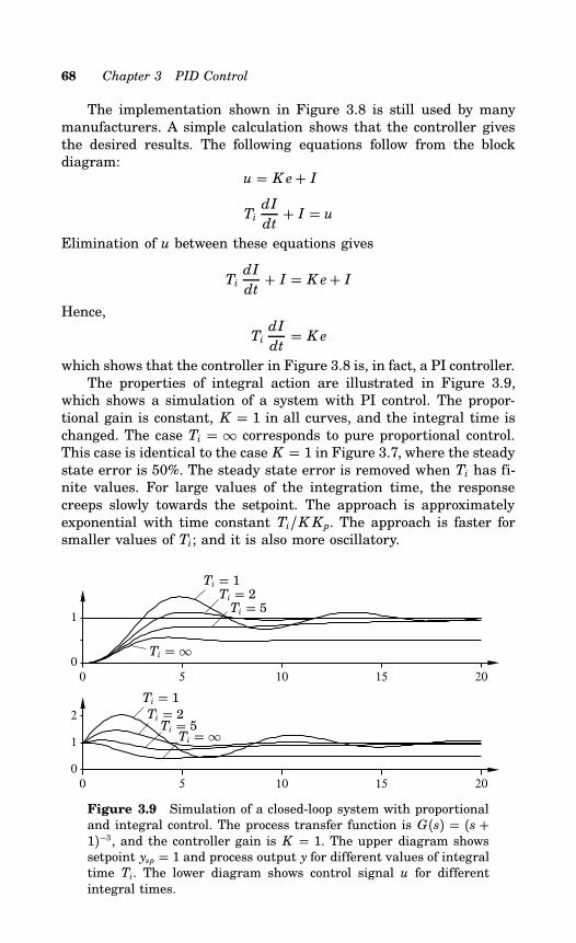
68 Chapter 3 PID Control
The implementation shown in Figure 3.8 is still used by manymanufacturers. A simple calculation shows that the controller givesthe desired results. The following equations follow from the blockdiagram:
u = K e+ I
TidI
dt+ I = u
Elimination of u between these equations gives
TidI
dt+ I = K e+ I
Hence,
TidI
dt= K e
which shows that the controller in Figure 3.8 is, in fact, a PI controller.The properties of integral action are illustrated in Figure 3.9,
which shows a simulation of a system with PI control. The propor-tional gain is constant, K = 1 in all curves, and the integral time ischanged. The case Ti = ∞ corresponds to pure proportional control.This case is identical to the case K = 1 in Figure 3.7, where the steadystate error is 50%. The steady state error is removed when Ti has fi-nite values. For large values of the integration time, the responsecreeps slowly towards the setpoint. The approach is approximatelyexponential with time constant Ti/K Kp. The approach is faster forsmaller values of Ti; and it is also more oscillatory.
0 5 10 15 200
1
0 5 10 15 200
1
2
Ti = 1Ti = 2Ti = 5
Ti = ∞
Ti = 1Ti = 2Ti = 5Ti = ∞
Figure 3.9 Simulation of a closed-loop system with proportionaland integral control. The process transfer function is G(s) = (s +1)−3, and the controller gain is K = 1. The upper diagram showssetpoint ysp = 1 and process output y for different values of integraltime Ti. The lower diagram shows control signal u for differentintegral times.
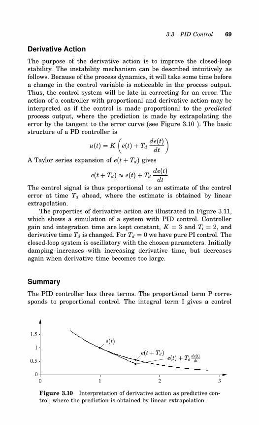
3.3 PID Control 69
Derivative Action
The purpose of the derivative action is to improve the closed-loopstability. The instability mechanism can be described intuitively asfollows. Because of the process dynamics, it will take some time beforea change in the control variable is noticeable in the process output.Thus, the control system will be late in correcting for an error. Theaction of a controller with proportional and derivative action may beinterpreted as if the control is made proportional to the predictedprocess output, where the prediction is made by extrapolating theerror by the tangent to the error curve (see Figure 3.10 ). The basicstructure of a PD controller is
u(t) = K(e(t) + Td de(t)
dt
)A Taylor series expansion of e(t+ Td) gives
e(t+ Td) e(t) + Td de(t)dt
The control signal is thus proportional to an estimate of the controlerror at time Td ahead, where the estimate is obtained by linearextrapolation.The properties of derivative action are illustrated in Figure 3.11,
which shows a simulation of a system with PID control. Controllergain and integration time are kept constant, K = 3 and Ti = 2, andderivative time Td is changed. For Td = 0 we have pure PI control. Theclosed-loop system is oscillatory with the chosen parameters. Initiallydamping increases with increasing derivative time, but decreasesagain when derivative time becomes too large.
Summary
The PID controller has three terms. The proportional term P corre-sponds to proportional control. The integral term I gives a control
0 1 2 30
0.5
1
1.5
e(t)e(t+ Td)
e(t) + Td de(t)dt
Figure 3.10 Interpretation of derivative action as predictive con-trol, where the prediction is obtained by linear extrapolation.
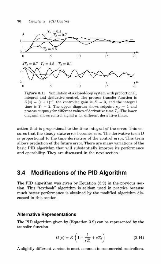
70 Chapter 3 PID Control
0 5 10 15 200
1
0 5 10 15 20−2
2
Td = 0.1Td = 0.7
Td = 4.5
Td = 0.7 Td = 4.5 Td = 0.1
Figure 3.11 Simulation of a closed-loop system with proportional,integral and derivative control. The process transfer function isG(s) = (s + 1)−3, the controller gain is K = 3, and the integraltime is Ti = 2. The upper diagram shows setpoint ysp = 1 andprocess output y for different values of derivative time Td. The lowerdiagram shows control signal u for different derivative times.
action that is proportional to the time integral of the error. This en-sures that the steady state error becomes zero. The derivative term Dis proportional to the time derivative of the control error. This termallows prediction of the future error. There are many variations of thebasic PID algorithm that will substantially improve its performanceand operability. They are discussed in the next section.
3.4 Modifications of the PID Algorithm
The PID algorithm was given by Equation (3.9) in the previous sec-tion. This “textbook” algorithm is seldom used in practice becausemuch better performance is obtained by the modified algorithm dis-cussed in this section.
Alternative Representations
The PID algorithm given by (Equation 3.9) can be represented by thetransfer function
G(s) = K(1+ 1sTi+ sTd
)(3.14)
A slightly different version is most common in commercial controllers.
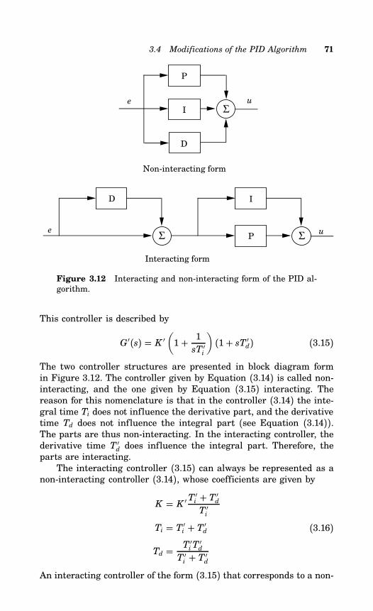
3.4 Modifications of the PID Algorithm 71
Σe u
Non-interacting form
P
D
I
Σ
D I
P Σ
Interacting form
e u
Figure 3.12 Interacting and non-interacting form of the PID al-gorithm.
This controller is described by
G ′(s) = K ′(1+ 1sT ′i
)(1+ sT ′d) (3.15)
The two controller structures are presented in block diagram formin Figure 3.12. The controller given by Equation (3.14) is called non-interacting, and the one given by Equation (3.15) interacting. Thereason for this nomenclature is that in the controller (3.14) the inte-gral time Ti does not influence the derivative part, and the derivativetime Td does not influence the integral part (see Equation (3.14)).The parts are thus non-interacting. In the interacting controller, thederivative time T ′d does influence the integral part. Therefore, theparts are interacting.The interacting controller (3.15) can always be represented as a
non-interacting controller (3.14), whose coefficients are given by
K = K ′T′i + T ′dT ′i
Ti = T ′i + T ′d
Td = T ′i T′d
T ′i + T ′d
(3.16)
An interacting controller of the form (3.15) that corresponds to a non-
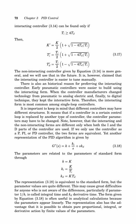
72 Chapter 3 PID Control
interacting controller (3.14) can be found only ifTi ≥ 4Td
Then,
K ′ = K2
(1+
√1− 4Td/Ti
)
T ′i =Ti
2
(1+
√1− 4Td/Ti
)
T ′d =Ti
2
(1−
√1− 4Td/Ti
)(3.17)
The non-interacting controller given by Equation (3.14) is more gen-eral, and we will use that in the future. It is, however, claimed thatthe interacting controller is easier to tune manually.There is also an historical reason for preferring the interacting
controller. Early pneumatic controllers were easier to build usingthe interacting form. When the controller manufacturers changedtechnology from pneumatic to analog electric and, finally, to digitaltechnique, they kept the interactive form. Therefore, the interactingform is most common among single-loop controllers.It is important to keep in mind that different controllers may have
different structures. It means that if a controller in a certain controlloop is replaced by another type of controller, the controller parame-ters may have to be changed. Note, however, that the interacting andthe non-interacting forms are different only when both the I and theD parts of the controller are used. If we only use the controller asa P, PI, or PD controller, the two forms are equivalent. Yet anotherrepresentation of the PID algorithm is given by
G ′′(s) = k+ kis+ skd (3.18)
The parameters are related to the parameters of standard formthrough
k = K
ki = KTi
kd = KTdThe representation (3.18) is equivalent to the standard form, but theparameter values are quite different. This may cause great difficultiesfor anyone who is not aware of the differences, particularly if parame-ter 1/ki is called integral time and kd derivative time. The form givenby Equation (3.18) is often useful in analytical calculations becausethe parameters appear linearly. The representation also has the ad-vantage that it is possible to obtain pure proportional, integral, orderivative action by finite values of the parameters.
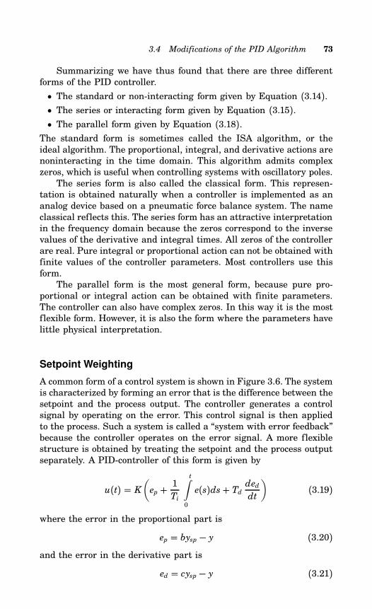
3.4 Modifications of the PID Algorithm 73
Summarizing we have thus found that there are three differentforms of the PID controller.
• The standard or non-interacting form given by Equation (3.14).• The series or interacting form given by Equation (3.15).• The parallel form given by Equation (3.18).The standard form is sometimes called the ISA algorithm, or theideal algorithm. The proportional, integral, and derivative actions arenoninteracting in the time domain. This algorithm admits complexzeros, which is useful when controlling systems with oscillatory poles.The series form is also called the classical form. This represen-
tation is obtained naturally when a controller is implemented as ananalog device based on a pneumatic force balance system. The nameclassical reflects this. The series form has an attractive interpretationin the frequency domain because the zeros correspond to the inversevalues of the derivative and integral times. All zeros of the controllerare real. Pure integral or proportional action can not be obtained withfinite values of the controller parameters. Most controllers use thisform.The parallel form is the most general form, because pure pro-
portional or integral action can be obtained with finite parameters.The controller can also have complex zeros. In this way it is the mostflexible form. However, it is also the form where the parameters havelittle physical interpretation.
Setpoint Weighting
A common form of a control system is shown in Figure 3.6. The systemis characterized by forming an error that is the difference between thesetpoint and the process output. The controller generates a controlsignal by operating on the error. This control signal is then appliedto the process. Such a system is called a “system with error feedback”because the controller operates on the error signal. A more flexiblestructure is obtained by treating the setpoint and the process outputseparately. A PID-controller of this form is given by
u(t) = K(ep + 1
Ti
t∫0
e(s)ds+ Td deddt
)(3.19)
where the error in the proportional part is
ep = bysp − y (3.20)and the error in the derivative part is
ed = cysp − y (3.21)
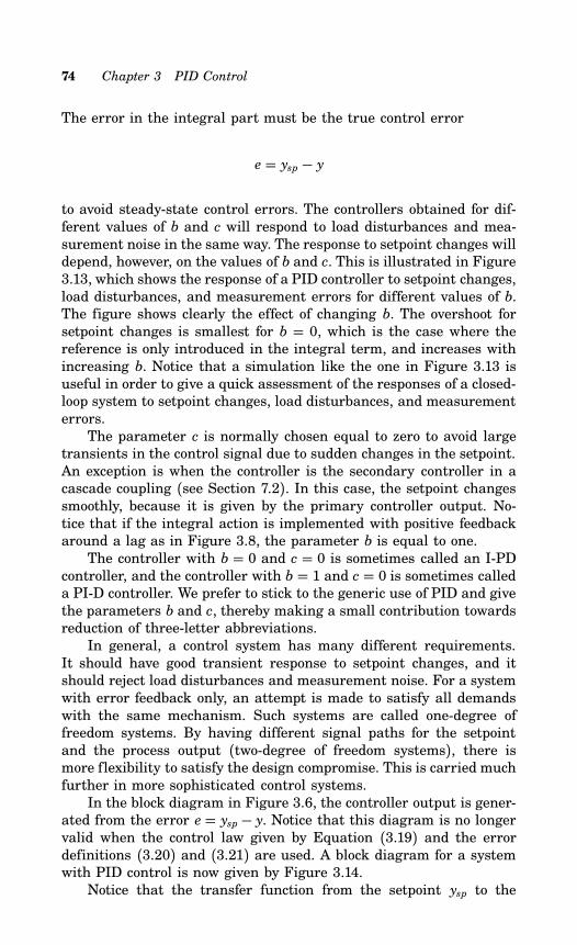
74 Chapter 3 PID Control
The error in the integral part must be the true control error
e = ysp − y
to avoid steady-state control errors. The controllers obtained for dif-ferent values of b and c will respond to load disturbances and mea-surement noise in the same way. The response to setpoint changes willdepend, however, on the values of b and c. This is illustrated in Figure3.13, which shows the response of a PID controller to setpoint changes,load disturbances, and measurement errors for different values of b.The figure shows clearly the effect of changing b. The overshoot forsetpoint changes is smallest for b = 0, which is the case where thereference is only introduced in the integral term, and increases withincreasing b. Notice that a simulation like the one in Figure 3.13 isuseful in order to give a quick assessment of the responses of a closed-loop system to setpoint changes, load disturbances, and measurementerrors.The parameter c is normally chosen equal to zero to avoid large
transients in the control signal due to sudden changes in the setpoint.An exception is when the controller is the secondary controller in acascade coupling (see Section 7.2). In this case, the setpoint changessmoothly, because it is given by the primary controller output. No-tice that if the integral action is implemented with positive feedbackaround a lag as in Figure 3.8, the parameter b is equal to one.The controller with b = 0 and c = 0 is sometimes called an I-PD
controller, and the controller with b = 1 and c = 0 is sometimes calleda PI-D controller. We prefer to stick to the generic use of PID and givethe parameters b and c, thereby making a small contribution towardsreduction of three-letter abbreviations.In general, a control system has many different requirements.
It should have good transient response to setpoint changes, and itshould reject load disturbances and measurement noise. For a systemwith error feedback only, an attempt is made to satisfy all demandswith the same mechanism. Such systems are called one-degree offreedom systems. By having different signal paths for the setpointand the process output (two-degree of freedom systems), there ismore flexibility to satisfy the design compromise. This is carried muchfurther in more sophisticated control systems.In the block diagram in Figure 3.6, the controller output is gener-
ated from the error e = ysp− y. Notice that this diagram is no longervalid when the control law given by Equation (3.19) and the errordefinitions (3.20) and (3.21) are used. A block diagram for a systemwith PID control is now given by Figure 3.14.Notice that the transfer function from the setpoint ysp to the
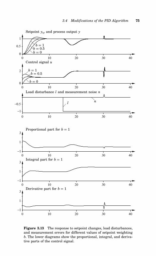
3.4 Modifications of the PID Algorithm 75
0 10 20 30 400
0.5
1
0 10 20 30 400
2
0 10 20 30 40
−1
−0.5
Setpoint ysp and process output y
Control signal u
Load disturbance l and measurement noise n
b = 1b = 0.5b = 0
b = 1b = 0.5
b = 0
ln
0 10 20 30 40−1
1
3
0 10 20 30 40−1
1
3
0 10 20 30 40−1
1
3
Proportional part for b = 1
Integral part for b = 1
Derivative part for b = 1
Figure 3.13 The response to setpoint changes, load disturbances,and measurement errors for different values of setpoint weightingb. The lower diagrams show the proportional, integral, and deriva-tive parts of the control signal.
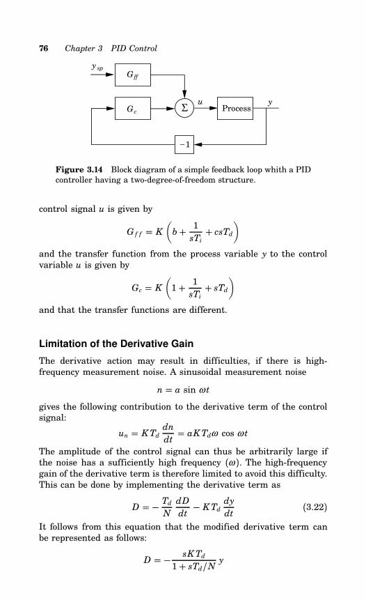
76 Chapter 3 PID Control
Processu y
Σ
1−
Gc
y sp
Gff
Figure 3.14 Block diagram of a simple feedback loop whith a PIDcontroller having a two-degree-of-freedom structure.
control signal u is given by
G f f = K(b+ 1sTi+ csTd
)
and the transfer function from the process variable y to the controlvariable u is given by
Gc = K(1+ 1sTi+ sTd
)
and that the transfer functions are different.
Limitation of the Derivative Gain
The derivative action may result in difficulties, if there is high-frequency measurement noise. A sinusoidal measurement noise
n = a sin ω t
gives the following contribution to the derivative term of the controlsignal:
un = KTd dndt= aKTdω cos ω t
The amplitude of the control signal can thus be arbitrarily large ifthe noise has a sufficiently high frequency (ω ). The high-frequencygain of the derivative term is therefore limited to avoid this difficulty.This can be done by implementing the derivative term as
D = − TdN
dD
dt− KTd dy
dt(3.22)
It follows from this equation that the modified derivative term canbe represented as follows:
D = − sKTd
1+ sTd/N y
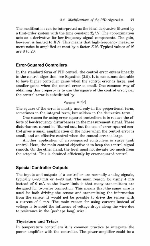
3.4 Modifications of the PID Algorithm 77
The modification can be interpreted as the ideal derivative filtered bya first-order system with the time constant Td/N. The approximationacts as a derivative for low-frequency signal components. The gain,however, is limited to KN. This means that high-frequency measure-ment noise is amplified at most by a factor KN. Typical values of Nare 8 to 20.
Error-Squared Controllers
In the standard form of PID control, the control error enters linearlyin the control algorithm, see Equation (3.9). It is sometimes desirableto have higher controller gains when the control error is large, andsmaller gains when the control error is small. One common way ofobtaining this property is to use the square of the control error, i.e.,the control error is substituted by
esquared = eeThe square of the error is mostly used only in the proportional term,sometimes in the integral term, but seldom in the derivative term.One reason for using error-squared controllers is to reduce the ef-
fects of low-frequency disturbances in the measurement signal. Thesedisturbances cannot be filtered out, but the use of error-squared con-trol gives a small amplification of the noise when the control error issmall, and an effective control when the control error is large.Another application of error-squared controllers is surge tank
control. Here, the main control objective is to keep the control signalsmooth. On the other hand, the level must not deviate too much fromthe setpoint. This is obtained efficiently by error-squared control.
Special Controller Outputs
The inputs and outputs of a controller are normally analog signals,typically 0–20 mA or 4–20 mA. The main reason for using 4 mAinstead of 0 mA as the lower limit is that many transmitters aredesigned for two-wire connection. This means that the same wire isused for both driving the sensor and transmitting the informationfrom the sensor. It would not be possible to drive the sensor witha current of 0 mA. The main reason for using current instead ofvoltage is to avoid the influence of voltage drops along the wire dueto resistance in the (perhaps long) wire.
Thyristors and Triacs
In temperature controllers it is common practice to integrate thepower amplifier with the controller. The power amplifier could be a
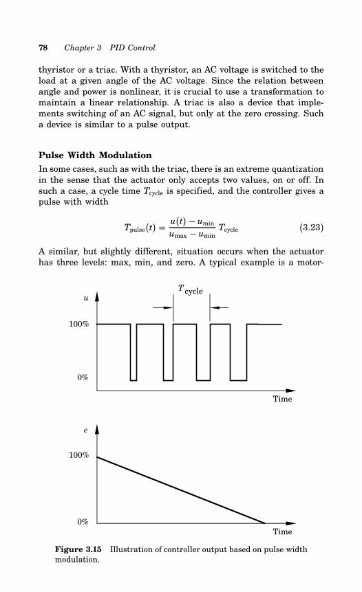
78 Chapter 3 PID Control
thyristor or a triac. With a thyristor, an AC voltage is switched to theload at a given angle of the AC voltage. Since the relation betweenangle and power is nonlinear, it is crucial to use a transformation tomaintain a linear relationship. A triac is also a device that imple-ments switching of an AC signal, but only at the zero crossing. Sucha device is similar to a pulse output.
Pulse Width Modulation
In some cases, such as with the triac, there is an extreme quantizationin the sense that the actuator only accepts two values, on or off. Insuch a case, a cycle time Tcycle is specified, and the controller gives apulse with width
Tpulse(t) = u(t) − uminumax − umin Tcycle (3.23)
A similar, but slightly different, situation occurs when the actuatorhas three levels: max, min, and zero. A typical example is a motor-
e
100%
0%
u
Time
Time
Tcycle
100%
0%
Figure 3.15 Illustration of controller output based on pulse widthmodulation.
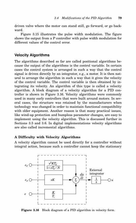
3.4 Modifications of the PID Algorithm 79
driven valve where the motor can stand still, go forward, or go back-ward.Figure 3.15 illustrates the pulse width modulation. The figure
shows the output from a P controller with pulse width modulation fordifferent values of the control error.
Velocity Algorithms
The algorithms described so far are called positional algorithms be-cause the output of the algorithms is the control variable. In certaincases the control system is arranged in such a way that the controlsignal is driven directly by an integrator, e.g., a motor. It is then nat-ural to arrange the algorithm in such a way that it gives the velocityof the control variable. The control variable is then obtained by in-tegrating its velocity. An algorithm of this type is called a velocityalgorithm. A block diagram of a velocity algorithm for a PID con-troller is shown in Figure 3.16. Velocity algorithms were commonlyused in many early controllers that were built around motors. In sev-eral cases, the structure was retained by the manufacturers whentechnology was changed in order to maintain functional compatibilitywith older equipment. Another reason is that many practical issues,like wind-up protection and bumpless parameter changes, are easy toimplement using the velocity algorithm. This is discussed further inSections 3.5 and 3.6. In digital implementations velocity algorithmsare also called incremental algorithms.
A Difficulty with Velocity Algorithms
A velocity algorithm cannot be used directly for a controller withoutintegral action, because such a controller cannot keep the stationary
ΣsK
du
dt
eK
Ti
s2KTd
1+ sTd / N ed
ep u1s
Externalintegrator
Figure 3.16 Block diagram of a PID algorithm in velocity form.
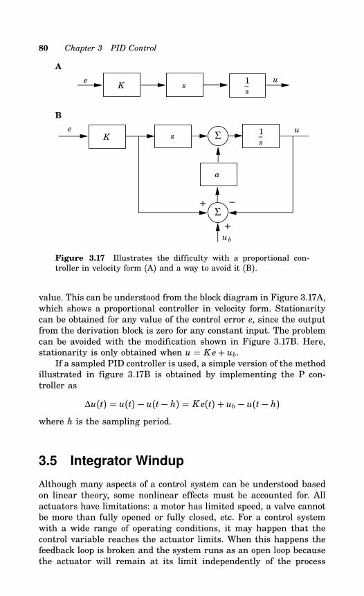
80 Chapter 3 PID Control
A
e uK s
1
s
B
e uΣ
1
sK s
a
ub
+ −
+
Σ
Figure 3.17 Illustrates the difficulty with a proportional con-troller in velocity form (A) and a way to avoid it (B).
value. This can be understood from the block diagram in Figure 3.17A,which shows a proportional controller in velocity form. Stationaritycan be obtained for any value of the control error e, since the outputfrom the derivation block is zero for any constant input. The problemcan be avoided with the modification shown in Figure 3.17B. Here,stationarity is only obtained when u = K e+ ub.If a sampled PID controller is used, a simple version of the method
illustrated in figure 3.17B is obtained by implementing the P con-troller as
∆u(t) = u(t) − u(t− h) = K e(t) + ub − u(t − h)where h is the sampling period.
3.5 Integrator Windup
Although many aspects of a control system can be understood basedon linear theory, some nonlinear effects must be accounted for. Allactuators have limitations: a motor has limited speed, a valve cannotbe more than fully opened or fully closed, etc. For a control systemwith a wide range of operating conditions, it may happen that thecontrol variable reaches the actuator limits. When this happens thefeedback loop is broken and the system runs as an open loop becausethe actuator will remain at its limit independently of the process
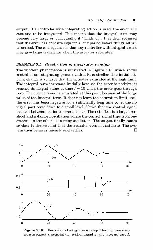
3.5 Integrator Windup 81
output. If a controller with integrating action is used, the error willcontinue to be integrated. This means that the integral term maybecome very large or, colloquially, it “winds up”. It is then requiredthat the error has opposite sign for a long period before things returnto normal. The consequence is that any controller with integral actionmay give large transients when the actuator saturates.
EXAMPLE 3.1 Illustration of integrator windup
The wind-up phenomenon is illustrated in Figure 3.18, which showscontrol of an integrating process with a PI controller. The initial set-point change is so large that the actuator saturates at the high limit.The integral term increases initially because the error is positive; itreaches its largest value at time t = 10 when the error goes throughzero. The output remains saturated at this point because of the largevalue of the integral term. It does not leave the saturation limit untilthe error has been negative for a sufficiently long time to let the in-tegral part come down to a small level. Notice that the control signalbounces between its limits several times. The net effect is a large over-shoot and a damped oscillation where the control signal flips from oneextreme to the other as in relay oscillation. The output finally comesso close to the setpoint that the actuator does not saturate. The sys-tem then behaves linearly and settles.
0 20 40 60 800
1
2
0 20 40 60 80
−0.1
0.1
0 20 40 60 80
−2
2
y
ysp
u
I
Figure 3.18 Illustration of integrator windup. The diagrams showprocess output y, setpoint ysp, control signal u, and integral part I.
82 Chapter 3 PID Control
Integrator windup may occur in connection with large setpointchanges or it may be caused by large disturbances or equipment mal-functions. Windup can also occur when selectors are used so that sev-eral controllers are driving one actuator. In cascade control, windupmay occur in the primary controller when the secondary controlleris switched to manual mode, uses its local setpoint, or if its controlsignal saturates. See Section 7.2.The phenomenon of windup was well known to manufacturers
of analog controllers who invented several tricks to avoid it. Theywere described under labels like preloading, batch unit, etc. Althoughthe problem was well understood, there were often limits imposedbecause of the analog implementations. The ideas were often keptas trade secrets and not much spoken about. The problem of windupwas rediscovered when controllers were implemented digitally andseveral methods to avoid windup were presented in the literature. Inthe following section we describe several of the ideas.
Setpoint Limitation
One way to try to avoid integrator windup is to introduce limiterson the setpoint variations so that the controller output will neverreach the actuator bounds. This often leads to conservative boundsand limitations on controller performance. Further, it does not avoidwindup caused by disturbances.
Incremental Algorithms
In the early phases of feedback control, integral action was integratedwith the actuator by having a motor drive the valve directly. In thiscase windup is handled automatically because integration stops whenthe valve stops. When controllers were implemented by analog tech-niques, and later with computers, many manufacturers used a con-figuration that was an analog of the old mechanical design. This ledto the so-called velocity algorithms discussed in Section 3.4. In thisalgorithm the rate of change of the control signal is first computedand then fed to an integrator. In some cases this integrator is a mo-tor directly connected to the actuator. In other cases the integratoris implemented internally in the controller. With this approach it iseasy to handle mode changes and windup. Windup is avoided by in-hibiting the integration whenever the output saturates. This methodis equivalent to back-calculation, which is described below. If the ac-tuator output is not measured, a model that computes the saturatedoutput can be used. It is also easy to limit the rate of change of thecontrol signal.
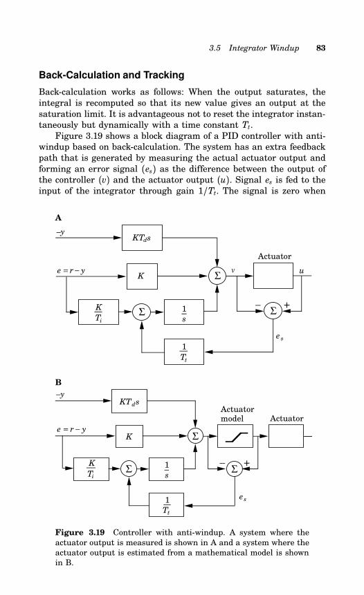
3.5 Integrator Windup 83
Back-Calculation and Tracking
Back-calculation works as follows: When the output saturates, theintegral is recomputed so that its new value gives an output at thesaturation limit. It is advantageous not to reset the integrator instan-taneously but dynamically with a time constant Tt.Figure 3.19 shows a block diagram of a PID controller with anti-
windup based on back-calculation. The system has an extra feedbackpath that is generated by measuring the actual actuator output andforming an error signal (es) as the difference between the output ofthe controller (v) and the actuator output (u). Signal es is fed to theinput of the integrator through gain 1/Tt. The signal is zero when
A
Σ
Actuator
–y
v u
– +
K Σ
Σ
e = r − y
1
Tt
K
Ti
KTds
1
s
e s
B
Actuator
– +Σ
Σ
Σ
e = r − y
KTds
K
1
s
1
Tt
K
Ti
–y
es
Actuatormodel
Figure 3.19 Controller with anti-windup. A system where theactuator output is measured is shown in A and a system where theactuator output is estimated from a mathematical model is shownin B.
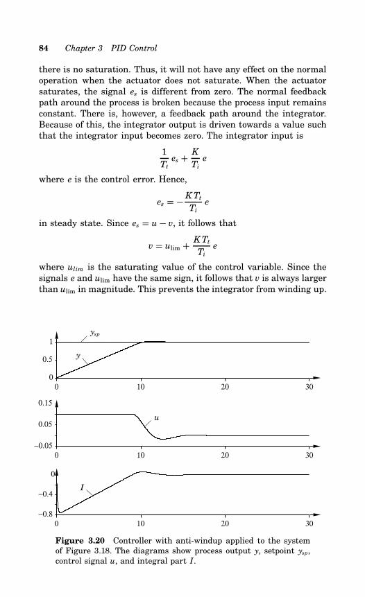
84 Chapter 3 PID Control
there is no saturation. Thus, it will not have any effect on the normaloperation when the actuator does not saturate. When the actuatorsaturates, the signal es is different from zero. The normal feedbackpath around the process is broken because the process input remainsconstant. There is, however, a feedback path around the integrator.Because of this, the integrator output is driven towards a value suchthat the integrator input becomes zero. The integrator input is
1Ttes + K
Tie
where e is the control error. Hence,
es = −KTtTie
in steady state. Since es = u− v, it follows that
v = ulim + KTtTie
where ulim is the saturating value of the control variable. Since thesignals e and ulim have the same sign, it follows that v is always largerthan ulim in magnitude. This prevents the integrator from winding up.
0 10 20 300
0.5
1
0 10 20 30−0.05
0.05
0.15
0 10 20 30−0.8
−0.4
0
ysp
y
u
I
Figure 3.20 Controller with anti-windup applied to the systemof Figure 3.18. The diagrams show process output y, setpoint ysp,control signal u, and integral part I.
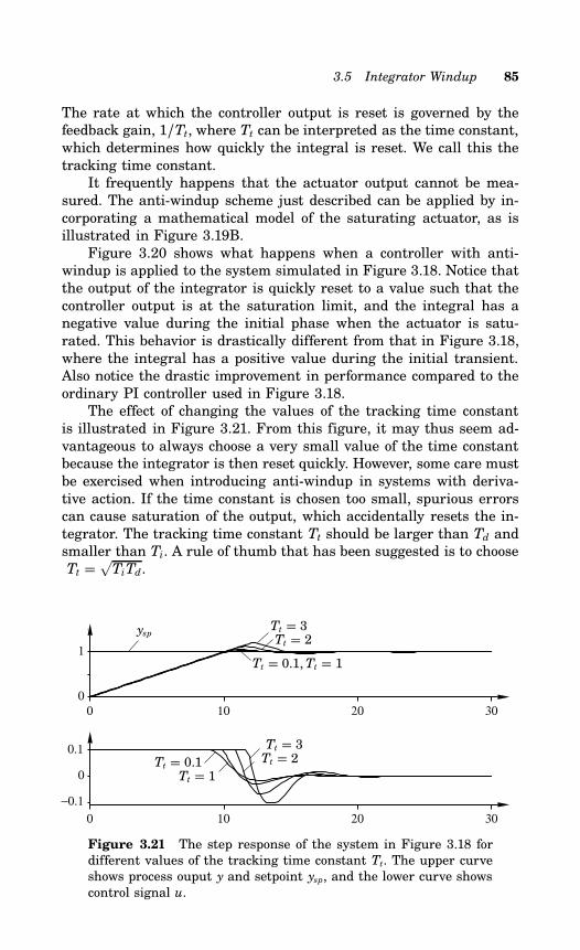
3.5 Integrator Windup 85
The rate at which the controller output is reset is governed by thefeedback gain, 1/Tt, where Tt can be interpreted as the time constant,which determines how quickly the integral is reset. We call this thetracking time constant.It frequently happens that the actuator output cannot be mea-
sured. The anti-windup scheme just described can be applied by in-corporating a mathematical model of the saturating actuator, as isillustrated in Figure 3.19B.Figure 3.20 shows what happens when a controller with anti-
windup is applied to the system simulated in Figure 3.18. Notice thatthe output of the integrator is quickly reset to a value such that thecontroller output is at the saturation limit, and the integral has anegative value during the initial phase when the actuator is satu-rated. This behavior is drastically different from that in Figure 3.18,where the integral has a positive value during the initial transient.Also notice the drastic improvement in performance compared to theordinary PI controller used in Figure 3.18.The effect of changing the values of the tracking time constant
is illustrated in Figure 3.21. From this figure, it may thus seem ad-vantageous to always choose a very small value of the time constantbecause the integrator is then reset quickly. However, some care mustbe exercised when introducing anti-windup in systems with deriva-tive action. If the time constant is chosen too small, spurious errorscan cause saturation of the output, which accidentally resets the in-tegrator. The tracking time constant Tt should be larger than Td andsmaller than Ti. A rule of thumb that has been suggested is to chooseTt =
√TiTd.
0 10 20 300
1
0 10 20 30
−0.1
0
0.1
ysp Tt = 3Tt = 2
Tt = 0.1,Tt = 1
Tt = 3Tt = 2
Tt = 1Tt = 0.1
Figure 3.21 The step response of the system in Figure 3.18 fordifferent values of the tracking time constant Tt. The upper curveshows process ouput y and setpoint ysp, and the lower curve showscontrol signal u.
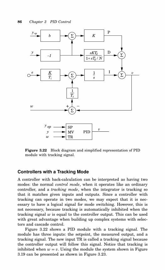
86 Chapter 3 PID Control
SP
MV
TR
PIDv
y
w
y sp
ΣvI
P
D
w
Σ
Σ
Σ
sKTd
1+ sTd / N
+ –Σ
1
Tt
1
s
K
y
e
b y sp
K
Ti
−1
Figure 3.22 Block diagram and simplified representation of PIDmodule with tracking signal.
Controllers with a Tracking Mode
A controller with back-calculation can be interpreted as having twomodes: the normal control mode, when it operates like an ordinarycontroller, and a tracking mode, when the integrator is tracking sothat it matches given inputs and outputs. Since a controller withtracking can operate in two modes, we may expect that it is nec-essary to have a logical signal for mode switching. However, this isnot necessary, because tracking is automatically inhibited when thetracking signal w is equal to the controller output. This can be usedwith great advantage when building up complex systems with selec-tors and cascade control.Figure 3.22 shows a PID module with a tracking signal. The
module has three inputs: the setpoint, the measured output, and atracking signal. The new input TR is called a tracking signal becausethe controller output will follow this signal. Notice that tracking isinhibited when w = v. Using the module the system shown in Figure3.19 can be presented as shown in Figure 3.23.
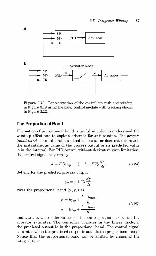
3.5 Integrator Windup 87
A
SP
MV
TR
PID Actuator
B
v u
Actuator model
SP
MV
TR
PID Actuator
Figure 3.23 Representation of the controllers with anti-windupin Figure 3.19 using the basic control module with tracking shownin Figure 3.22.
The Proportional Band
The notion of proportional band is useful in order to understand thewind-up effect and to explain schemes for anti-windup. The propor-tional band is an interval such that the actuator does not saturate ifthe instantaneous value of the process output or its predicted valueis in the interval. For PID control without derivative gain limitation,the control signal is given by
u = K (bysp − y) + I − KTd dydt
(3.24)Solving for the predicted process output
yp = y+ Td dydt
gives the proportional band (yl, yh) as
yl = bysp + I − umaxK
yh = bysp + I − uminK
(3.25)
and umin, umax are the values of the control signal for which theactuator saturates. The controller operates in the linear mode, ifthe predicted output is in the proportional band. The control signalsaturates when the predicted output is outside the proportional band.Notice that the proportional band can be shifted by changing theintegral term.
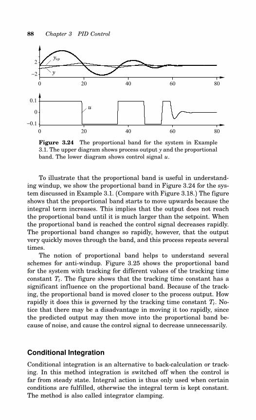
88 Chapter 3 PID Control
0 20 40 60 80
−2
2
0 20 40 60 80
−0.1
0
0.1
ysp
y
u
Figure 3.24 The proportional band for the system in Example3.1. The upper diagram shows process output y and the proportionalband. The lower diagram shows control signal u.
To illustrate that the proportional band is useful in understand-ing windup, we show the proportional band in Figure 3.24 for the sys-tem discussed in Example 3.1. (Compare with Figure 3.18.) The figureshows that the proportional band starts to move upwards because theintegral term increases. This implies that the output does not reachthe proportional band until it is much larger than the setpoint. Whenthe proportional band is reached the control signal decreases rapidly.The proportional band changes so rapidly, however, that the outputvery quickly moves through the band, and this process repeats severaltimes.The notion of proportional band helps to understand several
schemes for anti-windup. Figure 3.25 shows the proportional bandfor the system with tracking for different values of the tracking timeconstant Tt. The figure shows that the tracking time constant has asignificant influence on the proportional band. Because of the track-ing, the proportional band is moved closer to the process output. Howrapidly it does this is governed by the tracking time constant Tt. No-tice that there may be a disadvantage in moving it too rapidly, sincethe predicted output may then move into the proportional band be-cause of noise, and cause the control signal to decrease unnecessarily.
Conditional Integration
Conditional integration is an alternative to back-calculation or track-ing. In this method integration is switched off when the control isfar from steady state. Integral action is thus only used when certainconditions are fulfilled, otherwise the integral term is kept constant.The method is also called integrator clamping.
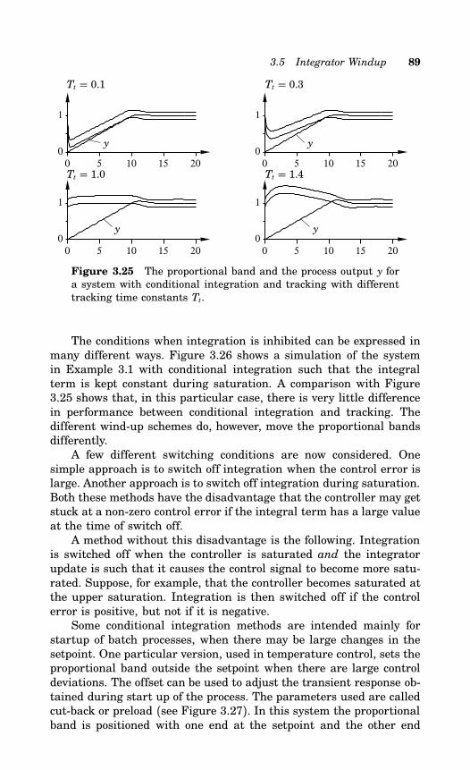
3.5 Integrator Windup 89
0 5 10 15 200
1
0 5 10 15 200
1
0 5 10 15 200
1
0 5 10 15 200
1
Tt = 0.1
Tt = 1.0
Tt = 0.3
Tt = 1.4
y y
y y
Figure 3.25 The proportional band and the process output y fora system with conditional integration and tracking with differenttracking time constants Tt.
The conditions when integration is inhibited can be expressed inmany different ways. Figure 3.26 shows a simulation of the systemin Example 3.1 with conditional integration such that the integralterm is kept constant during saturation. A comparison with Figure3.25 shows that, in this particular case, there is very little differencein performance between conditional integration and tracking. Thedifferent wind-up schemes do, however, move the proportional bandsdifferently.A few different switching conditions are now considered. One
simple approach is to switch off integration when the control error islarge. Another approach is to switch off integration during saturation.Both these methods have the disadvantage that the controller may getstuck at a non-zero control error if the integral term has a large valueat the time of switch off.A method without this disadvantage is the following. Integration
is switched off when the controller is saturated and the integratorupdate is such that it causes the control signal to become more satu-rated. Suppose, for example, that the controller becomes saturated atthe upper saturation. Integration is then switched off if the controlerror is positive, but not if it is negative.Some conditional integration methods are intended mainly for
startup of batch processes, when there may be large changes in thesetpoint. One particular version, used in temperature control, sets theproportional band outside the setpoint when there are large controldeviations. The offset can be used to adjust the transient response ob-tained during start up of the process. The parameters used are calledcut-back or preload (see Figure 3.27). In this system the proportionalband is positioned with one end at the setpoint and the other end
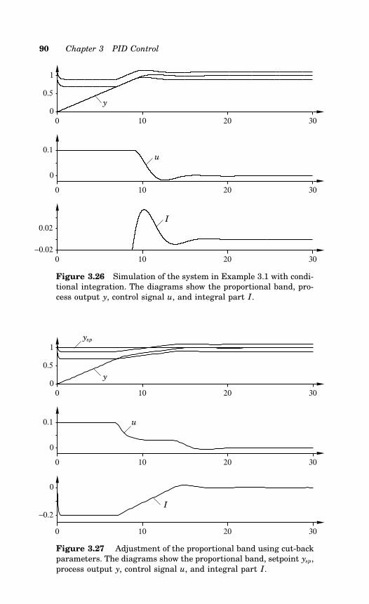
90 Chapter 3 PID Control
0 10 20 300
0.5
1
0 10 20 30
0
0.1
0 10 20 30−0.02
0.02
y
u
I
Figure 3.26 Simulation of the system in Example 3.1 with condi-tional integration. The diagrams show the proportional band, pro-cess output y, control signal u, and integral part I.
0 10 20 300
0.5
1
0 10 20 30
0
0.1
0 10 20 30
−0.2
0
ysp
y
u
I
Figure 3.27 Adjustment of the proportional band using cut-backparameters. The diagrams show the proportional band, setpoint ysp,process output y, control signal u, and integral part I.
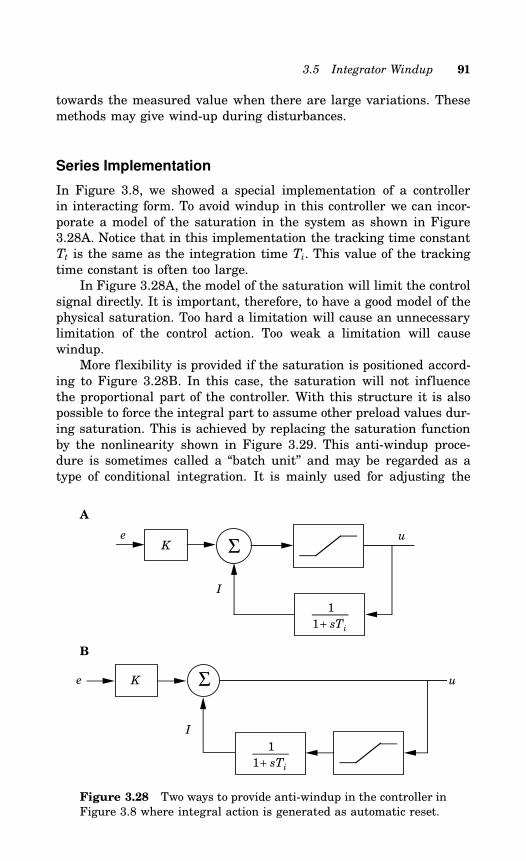
3.5 Integrator Windup 91
towards the measured value when there are large variations. Thesemethods may give wind-up during disturbances.
Series Implementation
In Figure 3.8, we showed a special implementation of a controllerin interacting form. To avoid windup in this controller we can incor-porate a model of the saturation in the system as shown in Figure3.28A. Notice that in this implementation the tracking time constantTt is the same as the integration time Ti. This value of the trackingtime constant is often too large.In Figure 3.28A, the model of the saturation will limit the control
signal directly. It is important, therefore, to have a good model of thephysical saturation. Too hard a limitation will cause an unnecessarylimitation of the control action. Too weak a limitation will causewindup.More flexibility is provided if the saturation is positioned accord-
ing to Figure 3.28B. In this case, the saturation will not influencethe proportional part of the controller. With this structure it is alsopossible to force the integral part to assume other preload values dur-ing saturation. This is achieved by replacing the saturation functionby the nonlinearity shown in Figure 3.29. This anti-windup proce-dure is sometimes called a “batch unit” and may be regarded as atype of conditional integration. It is mainly used for adjusting the
A
ΣKe
I
u
1
1+ sTi
B
1
1+ sTi
u
I
ΣKe
Figure 3.28 Two ways to provide anti-windup in the controller inFigure 3.8 where integral action is generated as automatic reset.
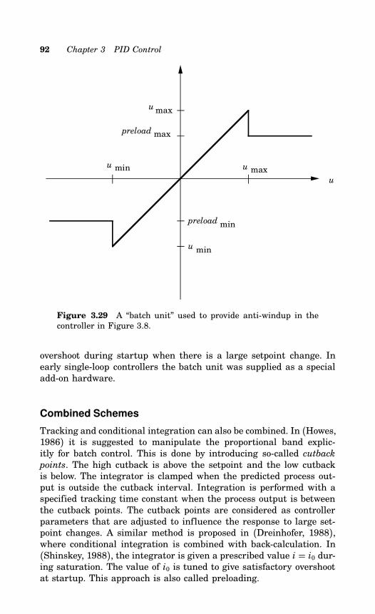
92 Chapter 3 PID Control
u
u min u max
u min
u max
maxpreload
preload min
Figure 3.29 A “batch unit” used to provide anti-windup in thecontroller in Figure 3.8.
overshoot during startup when there is a large setpoint change. Inearly single-loop controllers the batch unit was supplied as a specialadd-on hardware.
Combined Schemes
Tracking and conditional integration can also be combined. In (Howes,1986) it is suggested to manipulate the proportional band explic-itly for batch control. This is done by introducing so-called cutbackpoints. The high cutback is above the setpoint and the low cutbackis below. The integrator is clamped when the predicted process out-put is outside the cutback interval. Integration is performed with aspecified tracking time constant when the process output is betweenthe cutback points. The cutback points are considered as controllerparameters that are adjusted to influence the response to large set-point changes. A similar method is proposed in (Dreinhofer, 1988),where conditional integration is combined with back-calculation. In(Shinskey, 1988), the integrator is given a prescribed value i = i0 dur-ing saturation. The value of i0 is tuned to give satisfactory overshootat startup. This approach is also called preloading.
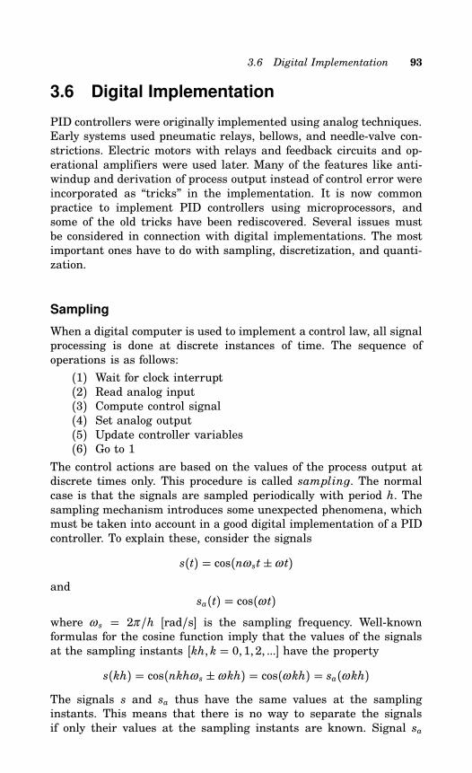
3.6 Digital Implementation 93
3.6 Digital Implementation
PID controllers were originally implemented using analog techniques.Early systems used pneumatic relays, bellows, and needle-valve con-strictions. Electric motors with relays and feedback circuits and op-erational amplifiers were used later. Many of the features like anti-windup and derivation of process output instead of control error wereincorporated as “tricks” in the implementation. It is now commonpractice to implement PID controllers using microprocessors, andsome of the old tricks have been rediscovered. Several issues mustbe considered in connection with digital implementations. The mostimportant ones have to do with sampling, discretization, and quanti-zation.
Sampling
When a digital computer is used to implement a control law, all signalprocessing is done at discrete instances of time. The sequence ofoperations is as follows:
(1) Wait for clock interrupt(2) Read analog input(3) Compute control signal(4) Set analog output(5) Update controller variables(6) Go to 1
The control actions are based on the values of the process output atdiscrete times only. This procedure is called samplin. The normalcase is that the signals are sampled periodically with period h. Thesampling mechanism introduces some unexpected phenomena, whichmust be taken into account in a good digital implementation of a PIDcontroller. To explain these, consider the signals
s(t) = cos(nω st±ω t)and
sa(t) = cos(ω t)where ω s = 2π/h [rad/s] is the sampling frequency. Well-knownformulas for the cosine function imply that the values of the signalsat the sampling instants [kh, k = 0, 1, 2, ...] have the property
s(kh) = cos(nkhω s ±ω kh) = cos(ω kh) = sa(ω kh)The signals s and sa thus have the same values at the samplinginstants. This means that there is no way to separate the signalsif only their values at the sampling instants are known. Signal sa
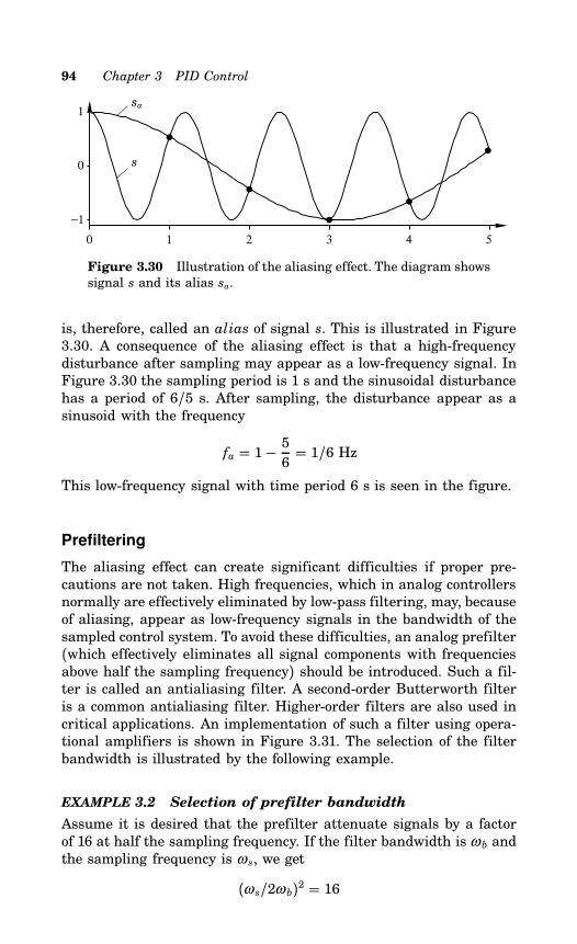
94 Chapter 3 PID Control
0 1 2 3 4 5
−1
0
1sa
s
Figure 3.30 Illustration of the aliasing effect. The diagram showssignal s and its alias sa.
is, therefore, called an alias of signal s. This is illustrated in Figure3.30. A consequence of the aliasing effect is that a high-frequencydisturbance after sampling may appear as a low-frequency signal. InFigure 3.30 the sampling period is 1 s and the sinusoidal disturbancehas a period of 6/5 s. After sampling, the disturbance appear as asinusoid with the frequency
fa = 1− 56 = 1/6 Hz
This low-frequency signal with time period 6 s is seen in the figure.
Prefiltering
The aliasing effect can create significant difficulties if proper pre-cautions are not taken. High frequencies, which in analog controllersnormally are effectively eliminated by low-pass filtering, may, becauseof aliasing, appear as low-frequency signals in the bandwidth of thesampled control system. To avoid these difficulties, an analog prefilter(which effectively eliminates all signal components with frequenciesabove half the sampling frequency) should be introduced. Such a fil-ter is called an antialiasing filter. A second-order Butterworth filteris a common antialiasing filter. Higher-order filters are also used incritical applications. An implementation of such a filter using opera-tional amplifiers is shown in Figure 3.31. The selection of the filterbandwidth is illustrated by the following example.
EXAMPLE 3.2 Selection of prefilter bandwidth
Assume it is desired that the prefilter attenuate signals by a factorof 16 at half the sampling frequency. If the filter bandwidth is ω b andthe sampling frequency is ω s, we get
(ω s/2ω b)2 = 16
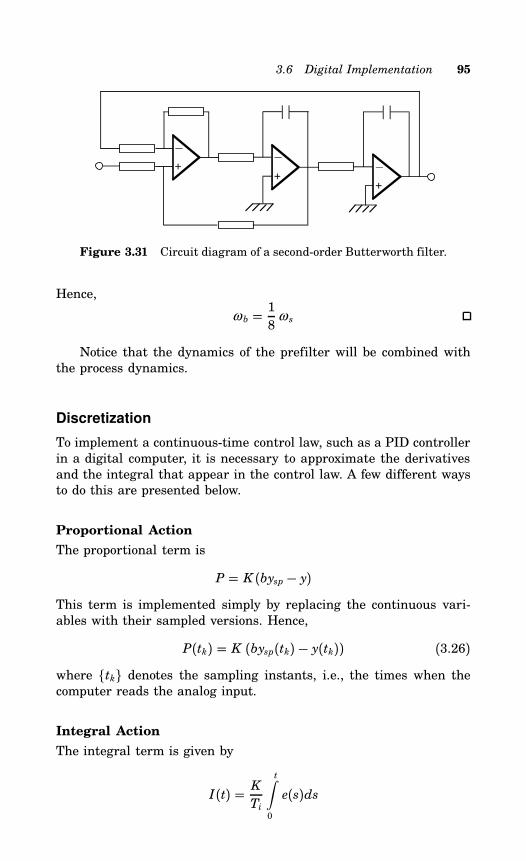
3.6 Digital Implementation 95
+
__
+_
+
Figure 3.31 Circuit diagram of a second-order Butterworth filter.
Hence,
ω b = 18 ω s
Notice that the dynamics of the prefilter will be combined withthe process dynamics.
Discretization
To implement a continuous-time control law, such as a PID controllerin a digital computer, it is necessary to approximate the derivativesand the integral that appear in the control law. A few different waysto do this are presented below.
Proportional Action
The proportional term is
P = K (bysp − y)This term is implemented simply by replacing the continuous vari-ables with their sampled versions. Hence,
P(tk) = K (bysp(tk) − y(tk)) (3.26)where tk denotes the sampling instants, i.e., the times when thecomputer reads the analog input.
Integral Action
The integral term is given by
I(t) = KTi
t∫0
e(s)ds
96 Chapter 3 PID Control
It follows thatdI
dt= KTie (3.27)
There are several ways of approximating this equation.
Forward differences: Approximating the derivative by a forwarddifference gives
I(tk+1) − I(tk)h
= KTie(tk)
This leads to the following recursive equation for the integral term
I(tk+1) = I(tk) + KhTie(tk) (3.28)
Backward differences: If the derivative in Equation (3.27) is ap-proximated instead by a backward difference, the following is ob-tained:
I(tk) − I(tk − 1)h
= KTie(tk)
This leads to the following recursive equation for the integral term
I(tk+1) = I(tk) + KhTie(tk+1) (3.29)
Tustin’s approximation and ramp equivalence: Another simpleapproximation method is due to Tustin. This approximation is
I(tk+1) = I(tk) + KhTi
e(tk+1) + e(tk)2
(3.30)
Yet another method is called ramp equivalence. This method gives ex-act outputs at the sampling instants, if the input signal is continuousand piece-wise linear between the sampling instants. The ramp equiv-alence method gives the same approximation of the integral term asthe Tustin approximation, i.e., Equation (3.30).Notice that all approximations have the same form, i.e.,
I(tk+1) = I(tk) + bi1e(tk+1) + bi2e(tk) (3.31)but with different values of parameters bi1 and bi2.
Derivative Action
The derivative term is given by Equation (3.22), i.e.,Td
N
dD
dt+ D = −KTd dy
dt(3.32)
This equation can be approximated in the same way as the integralterm.
3.6 Digital Implementation 97
Forward differences: Approximating the derivative by a forwarddifference gives
Td
N
D(tk+1) − D(tk)h
+ D(tk) = −KTd y(tk+1) − y(tk)h
This can be rewritten as
D(tk+1) =(1− Nh
Td
)D(tk) − KN (y(tk+1) − y(tk)) (3.33)
Backward differences: If the derivative in Equation (3.32) is ap-proximated by a backward difference, the following equation is ob-tained:
Td
N
D(tk) − D(tk−1)h
+ D(tk) = −KTd y(tk) − y(tk−1)h
This can be rewritten as
D(tk) = Td
Td + Nh D(tk−1) −KTdN
Td + Nh (y(tk) − y(tk−1)) (3.34)
Tustin’s approximation: Using the Tustin approximation to ap-proximate the derivative term gives
D(tk) = 2Td − Nh2Td + Nh D(tk−1) −2KTdN2Td + Nh (y(tk) − y(tk−1)) (3.35)
Ramp equivalence: Finally, the ramp equivalence approximationis
D(tk) = e−Nh/Td D(tk−1) − KTd(1− e−Nh/Td)
h(y(tk) − y(tk−1)) (3.36)
All approximations have the same form,
D(tk) = adD(tk−1) − bd (y(tk) − y(tk−1)) (3.37)but with different values of parameters ad and bd.The approximations of the derivative term are stable only when
ad < 1. The forward difference approximation requires that Td >Nh/2. The approximation becomes unstable for small values of Td.The other approximations are stable for all values of Td. Notice, how-ever, that Tustin’s approximation and the forward difference approx-imation give negative values of ad if Td is small. This is undesirablebecause the approximation will then exhibit ringing. The backwarddifference approximation will give good results for all values of Td. Itis also easier to compute than the ramp equivalence approximationand is, therefore, the most common method.
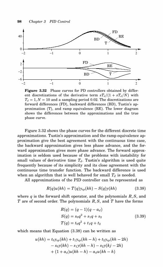
98 Chapter 3 PID Control
−2 −1 0 1 20
40
−2 −1 0 1 2−6
−2
2
FDRE
BDT
FD
BD
RE
T
Figure 3.32 Phase curves for PD controllers obtained by differ-ent discretizations of the derivative term sTd/(1 + sTd/N) withTd = 1,N = 10 and a sampling period 0.02. The discretizations areforward differences (FD), backward differences (BD), Tustin’s ap-proximation (T), and ramp equivalence (RE). The lower diagramshows the differences between the approximations and the truephase curve.
Figure 3.32 shows the phase curves for the different discrete timeapproximations. Tustin’s approximation and the ramp equivalence ap-proximation give the best agreement with the continuous time case,the backward approximation gives less phase advance, and the for-ward approximation gives more phase advance. The forward approx-imation is seldom used because of the problems with instability forsmall values of derivative time Td. Tustin’s algorithm is used quitefrequently because of its simplicity and its close agreement with thecontinuous time transfer function. The backward difference is usedwhen an algorithm that is well behaved for small Td is needed.All approximations of the PID controller can be represented as
R(q)u(kh) = T(q)ysp(kh) − S(q)y(kh) (3.38)where q is the forward shift operator, and the polynomials R,S, andT are of second order. The polynomials R,S, and T have the forms
R(q) = (q− 1)(q− ad)S(q) = s0q2 + s1q+ s2T(q) = t0q2 + t1q+ t2
(3.39)
which means that Equation (3.38) can be written asu(kh) = t0ysp(kh) + t1ysp(kh − h) + t2ysp(kh− 2h)
− s0y(kh) − s1y(kh− h) − s2y(kj − 2h)+ (1+ ad)u(kh − h) − adu(kh − h)
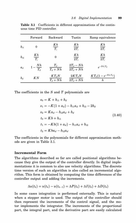
3.6 Digital Implementation 99
Table 3.1 Coefficients in different approximations of the contin-uous time PID controller.
Forward Backward Tustin Ramp equivalence
bi1 0Kh
Ti
Kh
2Ti
Kh
2Ti
bi2Kh
Ti0
Kh
2Ti
Kh
2Ti
ad 1− NhTd
Td
Td + Nh2Td − Nh2Td + Nh e−Nh/Td
bd K NKTdN
Td + Nh2KTdN2Td + Nh
KTd(1− e−Nh/Td )h
The coefficients in the S and T polynomials are
s0 = K + bi1 + bds1 = −K (1+ ad) − bi1ad + bi2 − 2bds2 = Kad − bi2ad + bdt0 = Kb+ bi1t1 = −Kb(1+ ad) − bi1ad + bi2t2 = Kbad − bi2ad
(3.40)
The coefficients in the polynomials for different approximation meth-ods are given in Table 3.1.
Incremental Form
The algorithms described so far are called positional algorithms be-cause they give the output of the controller directly. In digital imple-mentations it is common to also use velocity algorithms. The discretetime version of such an algorithm is also called an incremental algo-rithm. This form is obtained by computing the time differences of thecontroller output and adding the increments.
∆u(tk) = u(tk) − u(tk−1) = ∆P(tk) + ∆ I(tk) + ∆D(tk)In some cases integration is performed externally. This is naturalwhen a stepper motor is used. The output of the controller shouldthen represent the increments of the control signal, and the mo-tor implements the integrator. The increments of the proportionalpart, the integral part, and the derivative part are easily calculated
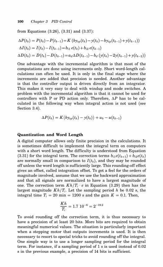
100 Chapter 3 PID Control
from Equations (3.26), (3.31) and (3.37):
∆P(tk) = P(tk)−P(tk−1)=K (bysp(tk)− y(tk)−bysp(tk−1)+ y(tk−1))∆ I(tk) = I(tk)− I(tk−1)=bi1 e(tk)+bi2 e(tk−1)
∆D(tk) = D(tk)−D(tk−1)=ad∆D(tk−1)−bd (y(tk)−2y(tk−1)+ y(tk−2))One advantage with the incremental algorithm is that most of thecomputations are done using increments only. Short word-length cal-culations can often be used. It is only in the final stage where theincrements are added that precision is needed. Another advantageis that the controller output is driven directly from an integrator.This makes it very easy to deal with windup and mode switches. Aproblem with the incremental algorithm is that it cannot be used forcontrollers with P or PD action only. Therefore, ∆P has to be cal-culated in the following way when integral action is not used (seeSection 3.4).
∆P(tk) = K(bysp(tk) − y(tk)
)+ ub − u(tk−1)
Quantization and Word Length
A digital computer allows only finite precision in the calculations. Itis sometimes difficult to implement the integral term on computerswith a short word length. The difficulty is understood from Equation(3.31) for the integral term. The correction terms bi1e(tk+1)+ bi2e(tk)are normally small in comparison to I(tk), and they may be roundedoff unless the word length is sufficiently large. This rounding-off effectgives an offset, called integration offset. To get a feel for the orders ofmagnitude involved, assume that we use the backward approximationand that all signals are normalized to have a largest magnitude ofone. The correction term Kh/Ti ⋅ e in Equation (3.29) then has thelargest magnitude Kh/Ti. Let the sampling period h be 0.02 s, theintegral time Ti = 20 min = 1200 s and the gain K = 0.1. Then,
Kh
Ti= 1.7 10−6 = 2−19.2
To avoid rounding off the correction term, it is thus necessary tohave a precision of at least 20 bits. More bits are required to obtainmeaningful numerical values. The situation is particularly importantwhen a stepping motor that outputs increments is used. It is thennecessary to resort to special tricks to avoid rounding off the integral.One simple way is to use a longer sampling period for the integralterm. For instance, if a sampling period of 1 s is used instead of 0.02s in the previous example, a precision of 14 bits is sufficient.
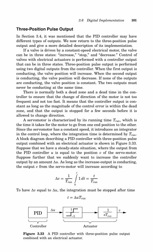
3.6 Digital Implementation 101
Three-Position Pulse Output
In Section 3.4, it was mentioned that the PID controller may havedifferent types of outputs. We now return to the three-position pulseoutput and give a more detailed description of its implementation.If a valve is driven by a constant-speed electrical motor, the valve
can be in three states: “increase,” “stop,” and “decrease.” Control ofvalves with electrical actuators is performed with a controller outputthat can be in three states. Three-position pulse output is performedusing two digital outputs from the controller. When the first output isconducting, the valve position will increase. When the second outputis conducting, the valve position will decrease. If none of the outputsare conducting, the valve position is constant. The two outputs mustnever be conducting at the same time.There is normally both a dead zone and a dead time in the con-
troller to ensure that the change of direction of the motor is not toofrequent and not too fast. It means that the controller output is con-stant as long as the magnitude of the control error is within the deadzone, and that the output is stopped for a few seconds before it isallowed to change direction.A servomotor is characterized by its running time Trun, which is
the time it takes for the motor to go from one end position to the other.Since the servomotor has a constant speed, it introduces an integratorin the control loop, where the integration time is determined by Trun.A block diagram describing a PID controller with three-position pulseoutput combined with an electrical actuator is shown in Figure 3.33.Suppose that we have a steady-state situation, where the output fromthe PID controller u is equal to the position v of the servo-motor.Suppose further that we suddenly want to increase the controlleroutput by an amount ∆u. As long as the increase-output is conducting,the output v from the servo-motor will increase according to
∆v = 1Trun
t∫0
1 dt = t
Trun
To have ∆v equal to ∆u, the integration must be stopped after time
t = ∆uTrun
PID1
–1
Controller Actuator
1
sTrun
v ∆u
Figure 3.33 A PID controller with three-position pulse outputcombined with an electrical actuator.
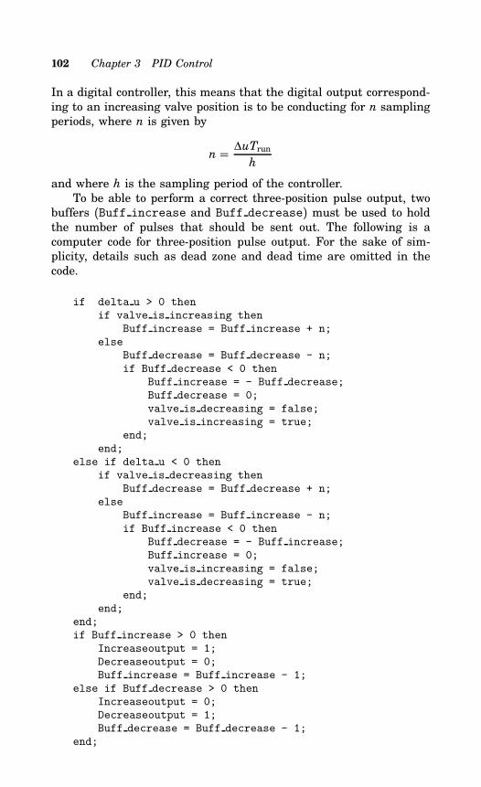
102 Chapter 3 PID Control
In a digital controller, this means that the digital output correspond-ing to an increasing valve position is to be conducting for n samplingperiods, where n is given by
n = ∆uTrun
h
and where h is the sampling period of the controller.To be able to perform a correct three-position pulse output, two
buffers (Buff increase and Buff decrease) must be used to holdthe number of pulses that should be sent out. The following is acomputer code for three-position pulse output. For the sake of sim-plicity, details such as dead zone and dead time are omitted in thecode.
if delta u > 0 thenif valve is increasing then
Buff increase = Buff increase + n;else
Buff decrease = Buff decrease - n;if Buff decrease < 0 then
Buff increase = - Buff decrease;Buff decrease = 0;valve is decreasing = false;valve is increasing = true;
end;end;
else if delta u < 0 thenif valve is decreasing then
Buff decrease = Buff decrease + n;else
Buff increase = Buff increase - n;if Buff increase < 0 then
Buff decrease = - Buff increase;Buff increase = 0;valve is increasing = false;valve is decreasing = true;
end;end;
end;if Buff increase > 0 then
Increaseoutput = 1;Decreaseoutput = 0;Buff increase = Buff increase - 1;
else if Buff decrease > 0 thenIncreaseoutput = 0;Decreaseoutput = 1;Buff decrease = Buff decrease - 1;
end;
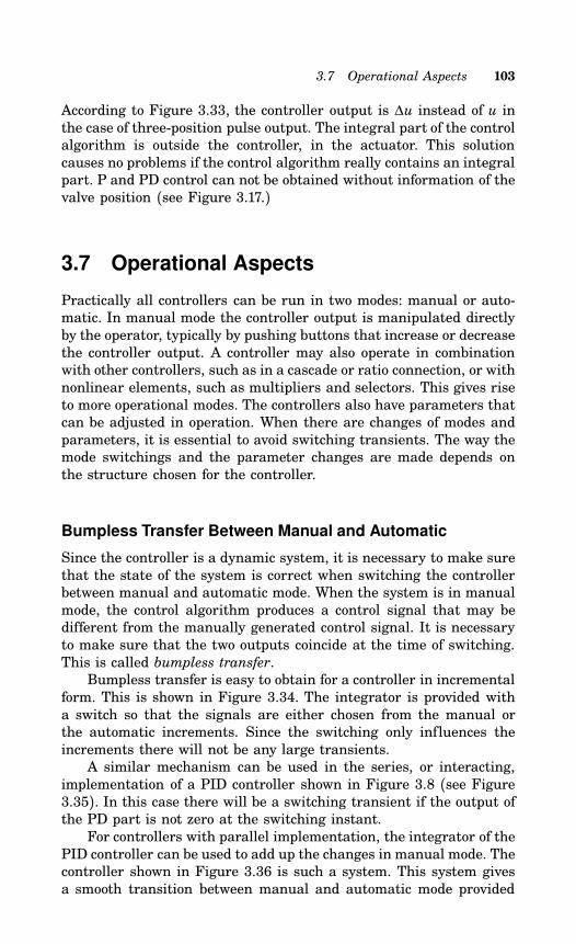
3.7 Operational Aspects 103
According to Figure 3.33, the controller output is ∆u instead of u inthe case of three-position pulse output. The integral part of the controlalgorithm is outside the controller, in the actuator. This solutioncauses no problems if the control algorithm really contains an integralpart. P and PD control can not be obtained without information of thevalve position (see Figure 3.17.)
3.7 Operational Aspects
Practically all controllers can be run in two modes: manual or auto-matic. In manual mode the controller output is manipulated directlyby the operator, typically by pushing buttons that increase or decreasethe controller output. A controller may also operate in combinationwith other controllers, such as in a cascade or ratio connection, or withnonlinear elements, such as multipliers and selectors. This gives riseto more operational modes. The controllers also have parameters thatcan be adjusted in operation. When there are changes of modes andparameters, it is essential to avoid switching transients. The way themode switchings and the parameter changes are made depends onthe structure chosen for the controller.
Bumpless Transfer Between Manual and Automatic
Since the controller is a dynamic system, it is necessary to make surethat the state of the system is correct when switching the controllerbetween manual and automatic mode. When the system is in manualmode, the control algorithm produces a control signal that may bedifferent from the manually generated control signal. It is necessaryto make sure that the two outputs coincide at the time of switching.This is called bumpless transfer.Bumpless transfer is easy to obtain for a controller in incremental
form. This is shown in Figure 3.34. The integrator is provided witha switch so that the signals are either chosen from the manual orthe automatic increments. Since the switching only influences theincrements there will not be any large transients.A similar mechanism can be used in the series, or interacting,
implementation of a PID controller shown in Figure 3.8 (see Figure3.35). In this case there will be a switching transient if the output ofthe PD part is not zero at the switching instant.For controllers with parallel implementation, the integrator of the
PID controller can be used to add up the changes in manual mode. Thecontroller shown in Figure 3.36 is such a system. This system givesa smooth transition between manual and automatic mode provided
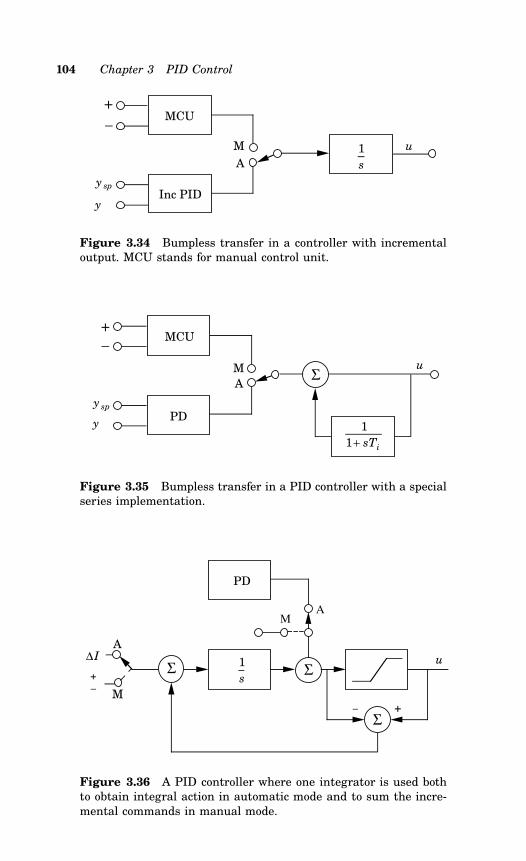
104 Chapter 3 PID Control
Inc PID
A
MCU+
–
M
1
s
u
y sp
y
Figure 3.34 Bumpless transfer in a controller with incrementaloutput. MCU stands for manual control unit.
PD
M
A
MCU
u
+
–
Σ
1
1+ sTi
y sp
y
Figure 3.35 Bumpless transfer in a PID controller with a specialseries implementation.
uΣ Σ
Σ
AM
A
M
PD
+
1
s
∆I
−
+
−
Figure 3.36 A PID controller where one integrator is used bothto obtain integral action in automatic mode and to sum the incre-mental commands in manual mode.
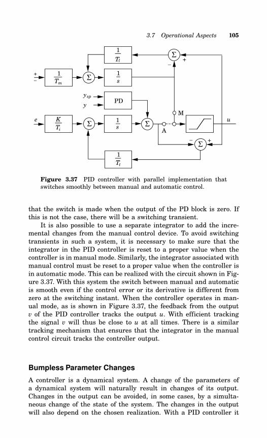
3.7 Operational Aspects 105
u
PD
e
– +
A
M
Σ Σ
Σ
K
Ti
1s
Σ
–+
Σ
+
−
1
Tm
1
Tt
1
s
1
Tt
ysp
y
Figure 3.37 PID controller with parallel implementation thatswitches smoothly between manual and automatic control.
that the switch is made when the output of the PD block is zero. Ifthis is not the case, there will be a switching transient.It is also possible to use a separate integrator to add the incre-
mental changes from the manual control device. To avoid switchingtransients in such a system, it is necessary to make sure that theintegrator in the PID controller is reset to a proper value when thecontroller is in manual mode. Similarly, the integrator associated withmanual control must be reset to a proper value when the controller isin automatic mode. This can be realized with the circuit shown in Fig-ure 3.37. With this system the switch between manual and automaticis smooth even if the control error or its derivative is different fromzero at the switching instant. When the controller operates in man-ual mode, as is shown in Figure 3.37, the feedback from the outputv of the PID controller tracks the output u. With efficient trackingthe signal v will thus be close to u at all times. There is a similartracking mechanism that ensures that the integrator in the manualcontrol circuit tracks the controller output.
Bumpless Parameter Changes
A controller is a dynamical system. A change of the parameters ofa dynamical system will naturally result in changes of its output.Changes in the output can be avoided, in some cases, by a simulta-neous change of the state of the system. The changes in the outputwill also depend on the chosen realization. With a PID controller it
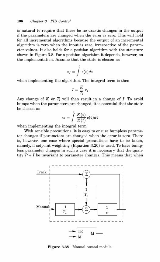
106 Chapter 3 PID Control
is natural to require that there be no drastic changes in the outputif the parameters are changed when the error is zero. This will holdfor all incremental algorithms because the output of an incrementalalgorithm is zero when the input is zero, irrespective of the param-eter values. It also holds for a position algorithm with the structureshown in Figure 3.8. For a position algorithm it depends, however, onthe implementation. Assume that the state is chosen as
xI =t∫e(τ )dτ
when implementing the algorithm. The integral term is then
I = KTixI
Any change of K or Ti will then result in a change of I. To avoidbumps when the parameters are changed, it is essential that the statebe chosen as
xI =t∫K (τ )Ti(τ ) e(τ )dτ
when implementing the integral term.With sensible precautions, it is easy to ensure bumpless parame-
ter changes if parameters are changed when the error is zero. Thereis, however, one case where special precautions have to be taken,namely, if setpoint weighting (Equation 3.20) is used. To have bump-less parameter changes in such a case it is necessary that the quan-tity P+ I be invariant to parameter changes. This means that when
Σ
ΣTrack
Manual
TR
MM
1
s
1
Tt
1
Tm
Figure 3.38 Manual control module.
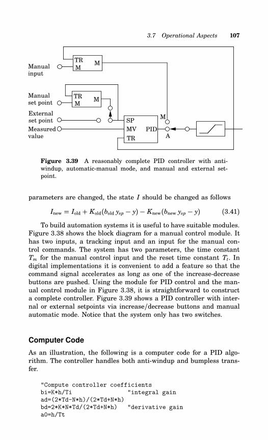
3.7 Operational Aspects 107
TR
MM
TR
MM
TR
MV
SP
PID
M
A
Manualinput
Manual set point
Externalset point
Measuredvalue
Figure 3.39 A reasonably complete PID controller with anti-windup, automatic-manual mode, and manual and external set-point.
parameters are changed, the state I should be changed as follows
Inew = Iold + Kold(bold ysp − y) − Knew(bnew ysp − y) (3.41)To build automation systems it is useful to have suitable modules.
Figure 3.38 shows the block diagram for a manual control module. Ithas two inputs, a tracking input and an input for the manual con-trol commands. The system has two parameters, the time constantTm for the manual control input and the reset time constant Tt. Indigital implementations it is convenient to add a feature so that thecommand signal accelerates as long as one of the increase-decreasebuttons are pushed. Using the module for PID control and the man-ual control module in Figure 3.38, it is straightforward to constructa complete controller. Figure 3.39 shows a PID controller with inter-nal or external setpoints via increase/decrease buttons and manualautomatic mode. Notice that the system only has two switches.
Computer Code
As an illustration, the following is a computer code for a PID algo-rithm. The controller handles both anti-windup and bumpless trans-fer.
"Compute controller coefficientsbi=K*h/Ti "integral gainad=(2*Td-N*h)/(2*Td+N*h)bd=2*K*N*Td/(2*Td+N*h) "derivative gaina0=h/Tt
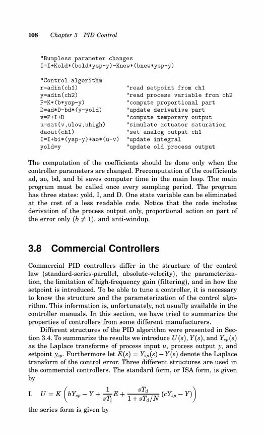
108 Chapter 3 PID Control
"Bumpless parameter changesI=I+Kold*(bold*ysp-y)-Knew*(bnew*ysp-y)
"Control algorithmr=adin(ch1) "read setpoint from ch1y=adin(ch2) "read process variable from ch2P=K*(b*ysp-y) "compute proportional partD=ad*D-bd*(y-yold) "update derivative partv=P+I+D "compute temporary outputu=sat(v,ulow,uhigh) "simulate actuator saturationdaout(ch1) "set analog output ch1I=I+bi*(ysp-y)+ao*(u-v) "update integralyold=y "update old process output
The computation of the coefficients should be done only when thecontroller parameters are changed. Precomputation of the coefficientsad, ao, bd, and bi saves computer time in the main loop. The mainprogram must be called once every sampling period. The programhas three states: yold, I, and D. One state variable can be eliminatedat the cost of a less readable code. Notice that the code includesderivation of the process output only, proportional action on part ofthe error only (b = 1), and anti-windup.
3.8 Commercial Controllers
Commercial PID controllers differ in the structure of the controllaw (standard-series-parallel, absolute-velocity), the parameteriza-tion, the limitation of high-frequency gain (filtering), and in how thesetpoint is introduced. To be able to tune a controller, it is necessaryto know the structure and the parameterization of the control algo-rithm. This information is, unfortunately, not usually available in thecontroller manuals. In this section, we have tried to summarize theproperties of controllers from some different manufacturers.Different structures of the PID algorithm were presented in Sec-
tion 3.4. To summarize the results we introduce U (s), Y(s), and Ysp(s)as the Laplace transforms of process input u, process output y, andsetpoint ysp. Furthermore let E(s) = Ysp(s)−Y(s) denote the Laplacetransform of the control error. Three different structures are used inthe commercial controllers. The standard form, or ISA form, is givenby
I. U = K(bYsp − Y + 1
sTiE + sTd
1+ sTd/N (cYsp − Y))
the series form is given by
3.9 When Can PID Control Be Used? 109
II. U = K ′((b+ 1sT ′i
) 1+ scT ′d1+ sT ′d/N
Ysp −(1+ 1sT ′i
) 1+ sT ′d1+ sT ′d/N
Y
)
and the parallel form by
III. U = K ′′ (bYsp − Y) + K′′i
sE + K ′′d s
1+ sK ′′d/(NK ′′)(cYsp − Y)
The relations between the different parameters are discussed in Sec-tion 3.4. Recall that the parameters b and c are the weightings thatinfluence the setpoint response. The values of b and c used are typi-cally 0 or 1 in commercial controllers. This does not use the power ofsetpoint weighting fully as was discussed in Section 3.4. The setpointweight factors b and c are chosen differently in different commercialcontrollers.The high-frequency gain of the derivative term is limited to avoid
noise amplification. This gain limitation can be parameterized interms of the parameter N.The sampling period is an important parameter of a digital PID
controller, which limits how fast processes can be controlled. Thevalues used in commercial controllers vary significantly.Table 3.2 summarizes the properties of some common commercial
PID controllers.
3.9 When Can PID Control Be Used?
The requirements on a control system may include many factors, suchas response to command signals, insensitivity to measurement noiseand process variations, and rejection of load disturbances. The designof a control system also involves aspects of process dynamics, actuatorsaturation, and disturbance characteristics. It may seem surprisingthat a controller as simple as the PID controller can work so well.The general empirical observation is that most industrial processescan be controlled reasonably well with PID control provided thatthe demands on the performance of the control are not too high.In the following paragraphs we delve further into this issue by firstconsidering cases where PID control is sufficient and then discussingsome generic problems where more sophisticated control is advisable.
When Is PI Control Sufficient?
Derivative action is frequently not used. It is an interesting observa-tion that many industrial controllers only have PI action and that inothers the derivative action can be (and frequently is) switched off.It can be shown that PI control is adequate for all processes where
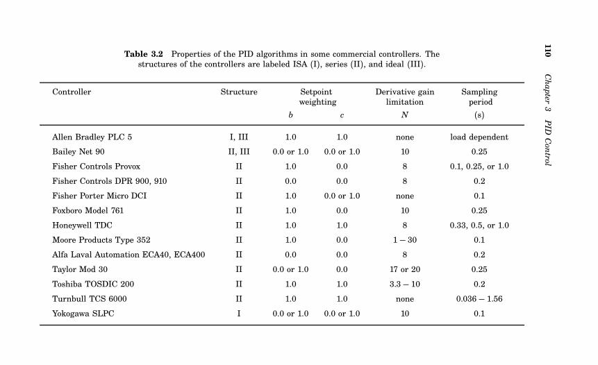
110
Chapter3PIDControl
Table 3.2 Properties of the PID algorithms in some commercial controllers. Thestructures of the controllers are labeled ISA (I), series (II), and ideal (III).
Controller Structure Setpoint Derivative gain Samplingweighting limitation period
b c N (s)
Allen Bradley PLC 5 I, III 1.0 1.0 none load dependent
Bailey Net 90 II, III 0.0 or 1.0 0.0 or 1.0 10 0.25
Fisher Controls Provox II 1.0 0.0 8 0.1, 0.25, or 1.0
Fisher Controls DPR 900, 910 II 0.0 0.0 8 0.2
Fisher Porter Micro DCI II 1.0 0.0 or 1.0 none 0.1
Foxboro Model 761 II 1.0 0.0 10 0.25
Honeywell TDC II 1.0 1.0 8 0.33, 0.5, or 1.0
Moore Products Type 352 II 1.0 0.0 1− 30 0.1
Alfa Laval Automation ECA40, ECA400 II 0.0 0.0 8 0.2
Taylor Mod 30 II 0.0 or 1.0 0.0 17 or 20 0.25
Toshiba TOSDIC 200 II 1.0 1.0 3.3− 10 0.2
Turnbull TCS 6000 II 1.0 1.0 none 0.036− 1.56Yokogawa SLPC I 0.0 or 1.0 0.0 or 1.0 10 0.1
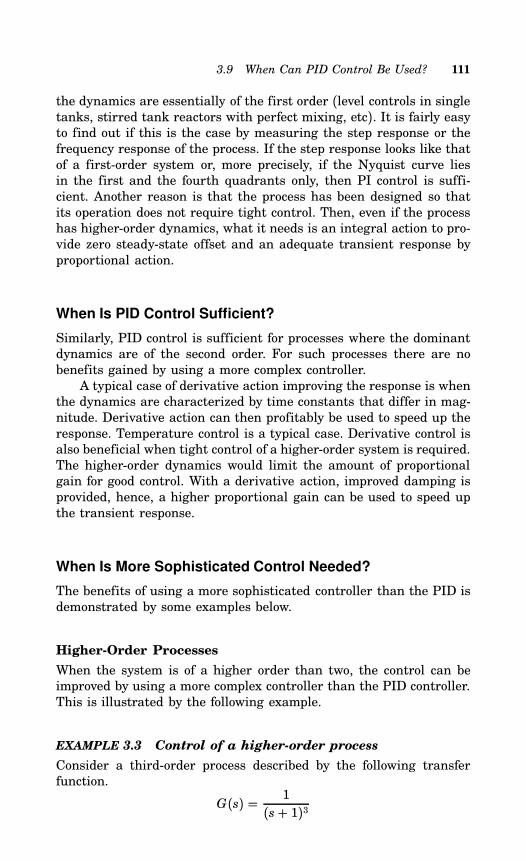
3.9 When Can PID Control Be Used? 111
the dynamics are essentially of the first order (level controls in singletanks, stirred tank reactors with perfect mixing, etc). It is fairly easyto find out if this is the case by measuring the step response or thefrequency response of the process. If the step response looks like thatof a first-order system or, more precisely, if the Nyquist curve liesin the first and the fourth quadrants only, then PI control is suffi-cient. Another reason is that the process has been designed so thatits operation does not require tight control. Then, even if the processhas higher-order dynamics, what it needs is an integral action to pro-vide zero steady-state offset and an adequate transient response byproportional action.
When Is PID Control Sufficient?
Similarly, PID control is sufficient for processes where the dominantdynamics are of the second order. For such processes there are nobenefits gained by using a more complex controller.A typical case of derivative action improving the response is when
the dynamics are characterized by time constants that differ in mag-nitude. Derivative action can then profitably be used to speed up theresponse. Temperature control is a typical case. Derivative control isalso beneficial when tight control of a higher-order system is required.The higher-order dynamics would limit the amount of proportionalgain for good control. With a derivative action, improved damping isprovided, hence, a higher proportional gain can be used to speed upthe transient response.
When Is More Sophisticated Control Needed?
The benefits of using a more sophisticated controller than the PID isdemonstrated by some examples below.
Higher-Order Processes
When the system is of a higher order than two, the control can beimproved by using a more complex controller than the PID controller.This is illustrated by the following example.
EXAMPLE 3.3 Control of a higher-order process
Consider a third-order process described by the following transferfunction.
G(s) = 1(s+ 1)3
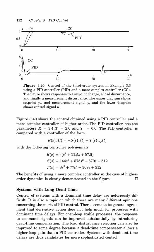
112 Chapter 3 PID Control
0 10 20 300
0.5
1
0 10 20 300
4
8
ysp CC
PID
CC
PID
Figure 3.40 Control of the third-order system in Example 3.3using a PID controller (PID) and a more complex controller (CC).The figure shows responses to a setpoint change, a load disturbance,and finally a measurement disturbance. The upper diagram showssetpoint ysp and measurement signal y, and the lower diagramshows control signal u.
Figure 3.40 shows the control obtained using a PID controller and amore complex controller of higher order. The PID controller has theparameters K = 3.4,Ti = 2.0 and Td = 0.6. The PID controller iscompared with a controller of the form
R(s)u(t) = −S(s)y(t) + T(s)ysp(t)with the following controller polynomials
R(s) = s(s2 + 11.5s+ 57.5)S(s) = 144s3 + 575s2 + 870s+ 512T(s) = 8s3 + 77s2 + 309s+ 512
The benefits of using a more complex controller in the case of higher-order dynamics is clearly demonstrated in the figure.
Systems with Long Dead Time
Control of systems with a dominant time delay are notoriously dif-ficult. It is also a topic on which there are many different opinionsconcerning the merit of PID control. There seems to be general agree-ment that derivative action does not help much for processes withdominant time delays. For open-loop stable processes, the responseto command signals can be improved substantially by introducingdead-time compensation. The load disturbance rejection can also beimproved to some degree because a dead-time compensator allows ahigher loop gain than a PID controller. Systems with dominant timedelays are thus candidates for more sophisticated control.
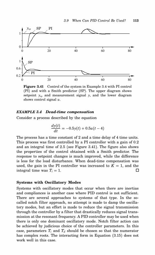
3.9 When Can PID Control Be Used? 113
0 20 40 60 800
1
0 20 40 60 800.2
0.6
1
ysp SP PI
SP
PI
Figure 3.41 Control of the system in Example 3.4 with PI control(PI) and with a Smith predictor (SP). The upper diagram showssetpoint ysp and measurement signal y, and the lower diagramshows control signal u.
EXAMPLE 3.4 Dead-time compensation
Consider a process described by the equation
dy(t)dt= −0.5y(t) + 0.5u(t− 4)
The process has a time constant of 2 and a time delay of 4 time units.This process was first controlled by a PI controller with a gain of 0.2and an integral time of 2.5 (see Figure 3.41). The figure also showsthe properties of the control obtained with a Smith predictor. Theresponse to setpoint changes is much improved, while the differenceis less for the load disturbance. When dead-time compensation wasused, the gain in the PI controller was increased to K = 1, and theintegral time was Ti = 1.
Systems with Oscillatory Modes
Systems with oscillatory modes that occur when there are inertiasand compliances is another case where PID control is not sufficient.There are several approaches to systems of that type. In the so-called notch filter approach, no attempt is made to damp the oscilla-tory modes, but an effort is made to reduce the signal transmissionthrough the controller by a filter that drastically reduces signal trans-mission at the resonant frequency. A PID controller may be used whenthere is only one dominant oscillatory mode. Notch filter action canbe achieved by judicious choice of the controller parameters. In thiscase, parameters Ti and Td should be chosen so that the numeratorhas complex roots. The interacting form in Equation (3.15) does notwork well in this case.
114 Chapter 3 PID Control
0 20 40 60
0
1
0 20 40 600
1
ysp
y
u
Figure 3.42 Response of the closed-loop system to setpoint andload disturbances. The graphs show setpoint ysp, process output y,and control signal u. The controller parameters are K = −0.25,Ti = −1, and b = 0.
EXAMPLE 3.5 PI control of a system with oscillatory modes
Consider for example a process with the transfer function
G(s) = ab2
(s+ a)(s2 + b2)where a = 1 and b = 5. The process has two undamped oscillatorypoles. If these poles are neglected, the process is simply a first-ordersystem that can conveniently be controlled by a PI controller. Attempt-ing to control the process with a PI controller, we find that controllerparameters K and Ti have to be negative. Reasonable values of theparameters are K = −0.25 and Ti = −1. Figure 3.42 shows the re-sponse of the closed-loop system to setpoint and load disturbances.Notice that the setpoint command does not excite the oscillatory polesso much. These modes are clearly visible, however, in the load distur-bance response. With a nonzero b the setpoint changes will also excitethe oscillatory modes, as is seen in Figure 3.43.
The system in Example 3.5 gives only moderate damping of theoscillatory modes. For systems where the oscillatory modes are insidethe servo bandwidth, it is necessary to have a controller with com-plex zeros. Such a controller can provide damping of the oscillatorymodes because the poles will be attracted to the controller zeros. Thecontroller zeros are the zeros of the function
1+ 1sTi+ sTd = Td
s
(s2 + 1
Tds+ 1TiTd
)(3.42)
Assume that the zeros correspond to the polynomial
s2 + 2ζ ω s+ω 2
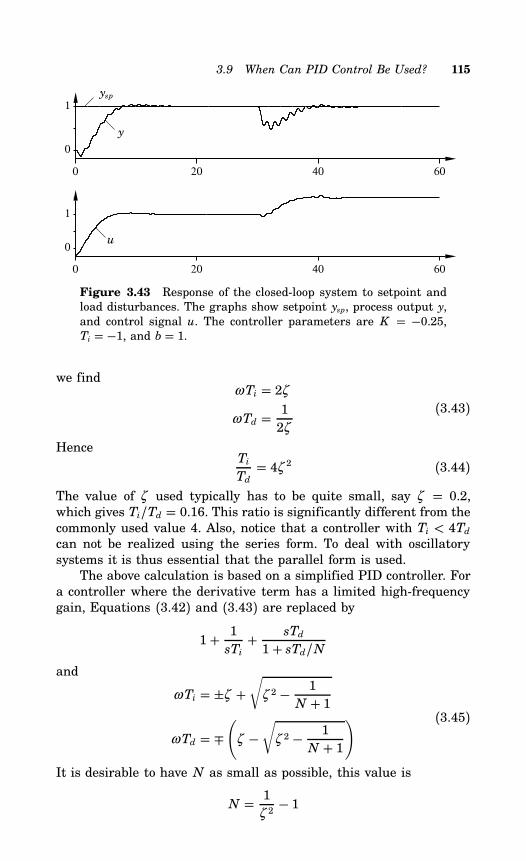
3.9 When Can PID Control Be Used? 115
0 20 40 60
0
1
0 20 40 60
0
1
ysp
y
u
Figure 3.43 Response of the closed-loop system to setpoint andload disturbances. The graphs show setpoint ysp, process output y,and control signal u. The controller parameters are K = −0.25,Ti = −1, and b = 1.
we findωTi = 2ζωTd = 1
2ζ
(3.43)
HenceTi
Td= 4ζ 2 (3.44)
The value of ζ used typically has to be quite small, say ζ = 0.2,which gives Ti/Td = 0.16. This ratio is significantly different from thecommonly used value 4. Also, notice that a controller with Ti < 4Tdcan not be realized using the series form. To deal with oscillatorysystems it is thus essential that the parallel form is used.The above calculation is based on a simplified PID controller. For
a controller where the derivative term has a limited high-frequencygain, Equations (3.42) and (3.43) are replaced by
1+ 1sTi+ sTd
1+ sTd/Nand
ωTi = ±ζ +√
ζ 2 − 1N + 1
ωTd = ∓(
ζ −√
ζ 2 − 1N + 1
) (3.45)
It is desirable to have N as small as possible, this value is
N = 1ζ 2− 1
116 Chapter 3 PID Control
which givesωTi = ζ
ωTd = Nζ(3.46)
HenceTi
Td= 1N= ζ 2
1− ζ 2(3.47)
For systems with oscillatory modes, the normal situation is that Ti ismuch smaller than Td. Notice also that the choice of parameter N iscritical for these applications.
Summary
When the dynamics of the process to be controlled are simple, a PIDcontroller is sufficient. When the dynamics become more complicated,the control performance can be improved by using a more sophisti-cated controller structure than the PID. Examples of such processeshave been given above. We end this section with some additional ex-amples.For some systems with large parameter variations it is possible to
design linear controllers that allow operation over a wide parameterrange. Such controllers are, however, often of high order.The control of process variables that are closely related to impor-
tant quality variables may be of a significant economic value. In suchcontrol loops it is frequently necessary to select the controller withrespect to the disturbance characteristics. This often leads to strate-gies that are not of the PID type. These problems are often associatedwith time delays.A general controller attempts to model the disturbances acting on
the system. Since a PID controller has limited complexity, it cannotmodel complex disturbance behavior in general nor periodic distur-bances in particular.
3.10 Conclusions
A detailed presentation of the PID algorithm has been given. Sev-eral modifications of the “textbook” version must be made to obtaina practical, useful controller. Problems that must be handled are, forexample, integral wind-up and introduction of setpoint values. In acomputer implementation, a discrete version of the PID algorithm isneeded. Several methods to derive discrete PID algorithms have beendescribed. Additional problems due to the sampling procedure must
3.11 References 117
be handled, such as the design of a prefilter to avoid aliasing. A dis-cussion of the limitations of the PID algorithm and a characterizationof processes where the PID controller manages to perform the controlhave also been given.
3.11 References
Proportional feedback in the form of a centrifugal governor was usedto regulate the speed of windmills around 1750. In 1788 James Wattused a similar system for speed control of steam engines. The benefitsof integral action was discovered a little later. Feedback control withproportional and integral action was rediscovered many times afterthat. In the early stages, the development of controllers was closelyrelated to development of sensors and actuators. Sensing, actuation,and control were often combined in the same device.The PID controller, in the form we know it today, emerged in
the period from 1915 to 1940. It coincided with the development oflegendary control companies such as Bristol, Fisher, Foxboro, Honey-well, Leeds & Northrup, and Taylor Instrument. Proportional andintegral action had been used for a long time. Integral action wasoften called automatic reset, because it replaced a manual reset thatwas used in proportional controllers to obtain the correct steady statevalue. The potential of a controller that could anticipate future controlerrors was discussed in the 1920s. However, it took some time beforethe idea could be implemented. A controller with derivative action wasintroduced by Ralph Clarridge of the Taylor Instrument Company in1935. At that time the function was called “pre-act.” An interestingoverview of the early history of PID controllers is given in (Stock, 198788). There is also much interesting material in publications from theinstrument companies. The interview with Nichols, who is one of thepioneers in our field, in (Blickley, 1990) gives a perspective on theearly development.It is interesting to observe that feedback was crucial for the con-
struction of the controller itself. The early pneumatic systems usedthe idea that an essentially linear controller can be obtained by afeedback loop composed of linear passive components and a nonlin-ear amplifier, the flapper valve. Similar ideas were used in electroniccontrollers with electric motors and relays.Many of the practically useful modifications of the controller first
appeared as special hardware functions. They were not expressed inmathematical form. An early mathematical analysis of a steam enginewith a governor was made in (Maxwell, 1868). This analysis clearlyshowed the difference between proportional and integral control. Thepapers (Minorsky, 1922), (Küpfmüller, 1928), (Nyquist, 1932), and
118 Chapter 3 PID Control
(Hazen, 1934) were available at the time when the PID controllerwas developed. However, there is little evidence that the engineers inthe process control field knew about them. Process control, therefore,developed independently. Two of the early papers were (Grebe et al.,1933), written by engineers at the Dow Chemical Company, (Ivanoff,1934), (Callender et al., 1936), and (Hartree et al., 1937).The PID controller has gone through an interesting development
because of the drastic technology changes that have happened since1940. The pneumatic controller improved drastically by making sys-tematic use of the force balance principle. Pneumatics was replacedby electronics when the operational amplifier appeared in the 1950s.A very significant development took place with the emergence of com-puter control in the 1960s. In the early computer control systems thecomputer commanded the setpoints of analog controllers. The nextstage of the development was direct digital control (DDC), where thecomputer was controlling the actuator directly, see (Webb, 1967). Adigital computer was then used to implement many PID controllers.This development led to a reconsideration of much of the fundamen-tals of PID control, see e.g. (Goff, 1966b), (L&N, 1968), (Moore et al.,1970), and (Palmor and Shinnar, 1979). The appearance of micro-processors in the 1970s made it possible to use digital control forsingle loop controllers, see (Stojić and Petrović, 1986). It also led tothe development of distributed control systems for process control,where the PID controller was a key element, see (Lukas, 1986). Asthe computing power of the microprocessors increased it was possibleto introduce tuning and adaptation in the single loop controllers. Thisdevelopment started in the 1980s and has accelerated in the 1990s,see (Åström et al., 1993).It is interesting to observe that many facts about PID control
were rediscovered in connection with the shifts in technology. Onereason being that many practical aspects of PID control were con-sidered as proprietory information that was not easily accessible inpublic literature. Much useful information was also scattered in theliterature.In spite of their wide spread use PID controllers are only treated
superficially in many textbooks and at university courses. The book(Shinskey, 1988) gives a good coverage. Implementation issues arediscussed in (Goff, 1966b), (Takahashi et al., 1972), (Clarke, 1984),(Åström and Wittenmark, 1990). The paper (Åström and Steingrímsson,1991) describes an implementation on a digital signal processor,which admits a very high sampling rate. The usefulness of a two-degree-of-freedom structure is discussed in (Horowitz, 1963). The ap-plication to PID control is treated in (Shigemasa et al., 1987).The phenomena of integral windup was well known in the early
analog implementations. The controller structures used were often
3.11 References 119
such that windup was avoided. The anti-windup schemes were redis-covered in connection with the development of direct digital control.This is discussed in (Fertik and Ross, 1967). Much work on avoid-ing windup have been done since then, and windup has now madeits way into some text books of control, see (Åström and Witten-mark, 1984). There are many papers written on the windup phe-nomena, see (Kramer and Jenkins, 1971), (Glattfelder and Schaufel-berger, 1983), (Krikelis, 1984), (Gallun et al., 1985), (Kapasourisand Athans, 1985), (Glattfelder and Schaufelberger, 1986), (Howes,1986), (Åström, 1987b), (Hanus et al., 1987), (Chen and Wang, 1988),(Glattfelder et al., 1988), (Hanus, 1988), (Zhang and Evans, 1988),(Åström and Rundqwist, 1989), (Rundqwist, 1990), and (Walgamaand Sternby, 1990). Mode switching is treated in the paper (Åström,1987b).The Smith predictor for control of systems with long time delays
was presented in (Smith, 1957). The papers (Ross, 1977) and (Meyeret al., 1976) compare the Smith predictor with the PID controller.
Controller Design
4.1 Introduction
This chapter describes some methods for determining the parame-ters of a PID controller. To obtain rational methods for designingcontrollers it is necessary to define the main purpose of the controlsystem. This is done in Section 4.2.The design methods differ with respect to the knowledge of the
process dynamics they require. A PI controller is described by twoparameters (K and Ti) and a PID controller by three or four pa-rameters (K , Ti, Td, and N). The classical Ziegler-Nichols methodsare discussed in Section 4.3. In these methods process dynamics arecharacterized by two parameters. One parameter is related to theprocess gain and the other describes how fast the process is. In thestep response method, the parameters are simple characteristics ob-tained from the step response. In the frequency response method, theparameters are the ultimate gain and the ultimate frequency.An obvious extension of the frequency response method is to de-
velop methods that are based on more knowledge of the open-looptransfer function, e.g., the slope of the transfer function or its valuesat two or more frequencies. In Section 4.4 we discuss various meth-ods that are based on attempts to shape the loop transfer function.Section 4.5 treats analytical design methods, where the controllertransfer function is obtained from the specifications and the processtransfer function by a direct calculation.One possibility for compromise between several different criteria
is to use optimization methods. This is discussed in Section 4.6. An-other way to characterize process dynamics with few parameters isto use low-order dynamic models with few parameters. Such methodsare discussed in Section 4.7 where the design goal is to position allthe poles of the closed-loop system. It is shown that methods basedon dynamic models of first and second order lead to PI and PID con-trollers.Instead of attempting to position all closed-loop poles, it can be at-
tempted to assign only a few dominating poles. Such methods are dis-
120
4.2 Specifications 121
cussed in Section 4.8. The approach leads to systematic design meth-ods and a unification of many other techniques. New simple designmethods based on the dominant pole design method are presented inChapter 5.In Section 4.9, design methods based on disturbance rejection are
presented. Finally, conclusions and references are given in Sections4.10 and 4.11.
4.2 Specifications
When solving a control problem it is necessary to understand whatthe primary goal of control is. Two common types of problems are tofollow the setpoint and to reject disturbances. It is also important tohave an assessment of the major restrictions, which can be
• System dynamics
• Nonlinearities
• Disturbances
• Process uncertainty
Typical specifications on a control system may include
• Attenuation of load disturbances
• Sensitivity to measurement noise
• Robustness to model uncertainty
• Setpoint following
Specifications can be expressed in many different ways. Features oftime responses for typical inputs is one possibility. Features of fre-quency responses or transfer functions are other possibilities. Someof the specifications such as attenuation and sensitivity to measure-ment errors, are conflicting, and others such as setpoint following andload disturbance rejection are nonconflicting.For process control applications setpoint following is often less
important than load disturbance attenuation. Setpoint changes areoften only made when the production rate is altered. Furthermore, theresponse to setpoint changes can be improved by feeding the setpointthrough ramping functions or by adjusting the setpoint weightingsdescribed in Section 3.4.
Load Disturbances
Load disturbances are disturbances that drive the process variablesaway from their desired values. Attenuation of load disturbances isof primary concern for process control. This is particularly the case
122 Chapter 4 Controller Design
for regulation problems where the processes are running in steadystate with constant setpoint for a long time. Load disturbances areoften of low frequencies. Step signals are often used as prototype dis-turbances. The disturbances may enter the system in many differentways. If nothing else is known, it is often assumed that the distur-bances enter at the process input. Typical responses due to a unitstep disturbance at the process input are shown in Figure 4.1. Thecharacteristics of the graphs in Figure 4.1 are often used to specifythe response to load disturbances. Let e be the error caused by a unitstep disturbance at the process input. Typical quantities used to char-acterize the error are: maximum error emax, time to reach maximumtmax, settling time ts, decay ratio d, and the integrated absolute error,which is defined by
IAE =∫ ∞
0e(t)dt (4.1)
The criterion IAE is in many cases a natural choice, at least forcontrol of quality variables. A severe drawback is that its evaluationrequires significant computations or a simulation of the process. Thesimulation must also be made with sufficient accuracy. Since the cri-terion is based on an infinite integral it is also necessary to simulatefor a long time.For processes that are nonoscillatory, IAE is the same as the
integrated error
IE =∫ ∞
0e(t)dt (4.2)
The quantity IE is a good approximation of IAE for systems that areoscillatory but well damped. The reason for using IE is that its valueis directly related to the controller parameters. To see this assumethat the control law is
u(t) = ke(t) + ki∫ t
0e(t)dt− kd dy
dt
and that this controller gives a stable closed-loop system. Further-more assume that the error is initially zero and that a unit stepdisturbance is applied at the process input. Since the closed-loop sys-tem is stable and has integral action the control error will go to zero.We thus find
u(∞) − u(0) = ki∫ ∞
0e(t)dt
Since the disturbance is applied at the process input, the change incontrol signal is equal to the change of the disturbance. Hence,
IE =∫ ∞
0e(t)dt = 1
ki= TiK
(4.3)
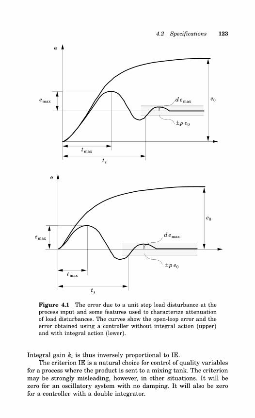
4.2 Specifications 123
e
emax
tmax
ts
e0
± p e0
d emax
emax
e0
ts
tmax
e
± p e0
d emax
Figure 4.1 The error due to a unit step load disturbance at theprocess input and some features used to characterize attenuationof load disturbances. The curves show the open-loop error and theerror obtained using a controller without integral action (upper)and with integral action (lower).
Integral gain ki is thus inversely proportional to IE.The criterion IE is a natural choice for control of quality variables
for a process where the product is sent to a mixing tank. The criterionmay be strongly misleading, however, in other situations. It will bezero for an oscillatory system with no damping. It will also be zerofor a controller with a double integrator.
124 Chapter 4 Controller Design
The quadratic criterion
ISE =∫ ∞
0e2(t)dt (4.4)
is also easy to compute. It has, however, the disadvantage that itgives a very high weight to large errors, which often leads to a poorlydamped closed loop.
Sensitivity to Measurement Noise
Measurement noise is typically of high frequency. Care should alwaysbe taken to reduce noise by appropriate filtering. For sampled systemsit is also important to choose the sampling rate properly. Measure-ment noise will be fed into the system through the feedback. It willgenerate control actions and control errors. The transmission of mea-surement noise to control actions can be described by the transferfunction
Gnu = Gc
1+ G (4.5)
where Gp is the process transfer function, Gc is the controller transferfunction, and G = GpGc is the loop transfer function. The transferfunction from measurement noise to process output is
Gny = 11+ G = S (4.6)
where S is called the sensitivity function. Since the magnitude ofG normally is small for high frequencies, we have approximatelyGnu = Gc for high frequencies.The high-frequency gain of a PID controller is
Khf = K (1+ N) (4.7)Notice that N = 0 corresponds to PI control. Multiplication of themeasurement noise by Kh f gives the fluctuations in the control signalthat are caused by the measurement noise. Also notice that theremay be a significant difference in Kh f for PI and PID control. It istypically an order of magnitude larger for a PID controller, since thegain normally is higher for a PID controller than for a PI controller,and N is typically around 10.
Sensitivity to Process Characteristics
The controller parameters are typically matched to the process char-acteristics. Since the process may change it is important that the
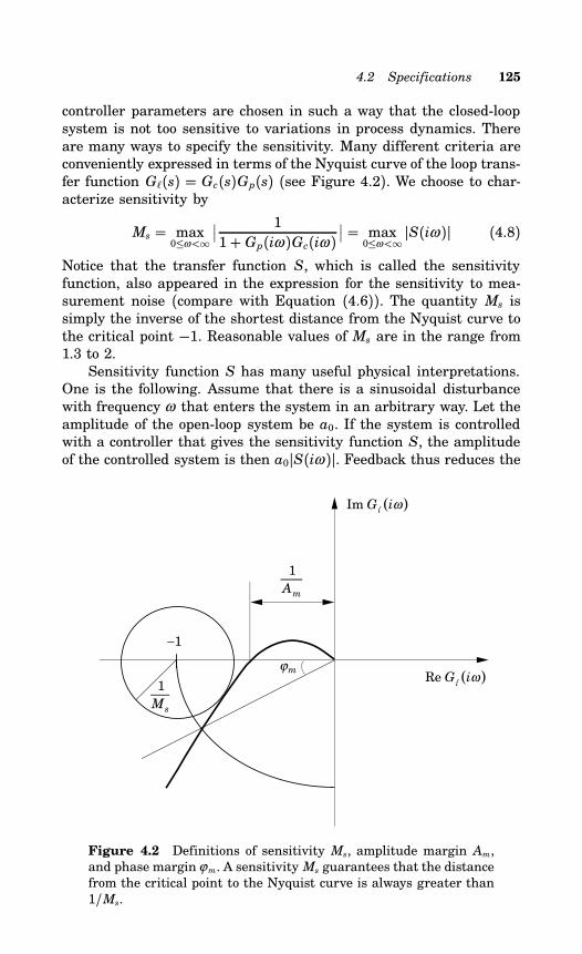
4.2 Specifications 125
controller parameters are chosen in such a way that the closed-loopsystem is not too sensitive to variations in process dynamics. Thereare many ways to specify the sensitivity. Many different criteria areconveniently expressed in terms of the Nyquist curve of the loop trans-fer function G(s) = Gc(s)Gp(s) (see Figure 4.2). We choose to char-acterize sensitivity by
Ms = max0≤ω<∞
∣∣ 11+ Gp(iω )Gc(iω )
∣∣ = max0≤ω<∞
S(iω ) (4.8)
Notice that the transfer function S, which is called the sensitivityfunction, also appeared in the expression for the sensitivity to mea-surement noise (compare with Equation (4.6)). The quantity Ms issimply the inverse of the shortest distance from the Nyquist curve tothe critical point −1. Reasonable values of Ms are in the range from1.3 to 2.Sensitivity function S has many useful physical interpretations.
One is the following. Assume that there is a sinusoidal disturbancewith frequency ω that enters the system in an arbitrary way. Let theamplitude of the open-loop system be a0. If the system is controlledwith a controller that gives the sensitivity function S, the amplitudeof the controlled system is then a0S(iω ). Feedback thus reduces the
−1
1
Ms
1
Am
ϕm
Im G iω( )
Re G iω( )l
l
Figure 4.2 Definitions of sensitivity Ms, amplitude margin Am,and phase marginϕm. A sensitivity Ms guarantees that the distancefrom the critical point to the Nyquist curve is always greater than1/Ms.
126 Chapter 4 Controller Design
effect of the disturbance if S(iω ) < 1, and it amplifies a disturbanceif S(iω ) > 1.Under very general assumptions it can be shown that the sensitiv-
ity can not be smaller than one for all frequencies. With a controllerhaving integral action we have S(0) = 0. Low frequency disturbancesthus can be reduced effectively with such a controller. When design-ing a controller it is important to be aware of the frequencies wheredisturbances are amplified. It is also important that the largest valueof the sensitivity is limited. It is common to require that the maxi-mum value of the sensitivity function, Ms be in the range of 1.3 to2.Amplitude margin (Am) and phase margin (ϕm) are other com-
mon sensitivity measures. They are defined as
Am = 1G(iωu)
ϕm = π + argG(iω )(4.9)
where the ultimate frequency ωu is the frequency where argG(iω ) =−π and the gain cross-over frequency ω is the frequency whereG(iω ) = 1. See Figure 4.2. The amplitude margin is also calledgain margin. We have the following relations
Am > Ms
Ms − 1ϕm > 2 arcsin 1
2Ms
(4.10)
Typical values of ϕm range from 30 to 60. Amplitude margins couldtypically vary from 2 to 5. A geometrical interpretation of the criteriongiven by Equation (4.8) is that the Nyquist curve of the loop transferfunction is always outside a circle around the critical point −1 withthe radius 1/Ms. An engineering interpretation is that the systemremains stable even if the gain is increased by the factor Ms/(Ms−1)or decreased by the vector Ms/(Ms + 1). The closed loop will remainstable even if a nonlinearity characterized by
xMs/(Ms + 1) < f (x) < xMs/(Ms − 1)is inserted in the loop. A small value of Ms thus ensures that the sys-tem will remain stable in spite of nonlinear actuator characteristics.
Setpoint Following
Specifications on setpoint following may include requirements on risetime, settling time, decay ratio, overshoot, and steady-state offset forstep changes in setpoint. See Figure 4.3. These quantities are definedin different ways and there are also different standards.
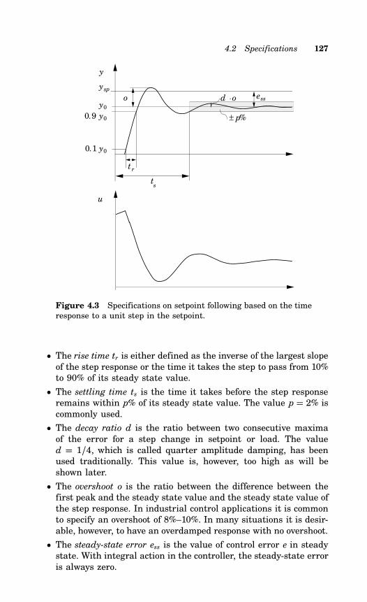
4.2 Specifications 127
y
tr
ts
o d ⋅o
u
± p%
ess
0.9 y0
0.1 y0
y0
ysp
Figure 4.3 Specifications on setpoint following based on the timeresponse to a unit step in the setpoint.
• The rise time tr is either defined as the inverse of the largest slopeof the step response or the time it takes the step to pass from 10%to 90% of its steady state value.
• The settling time ts is the time it takes before the step responseremains within p% of its steady state value. The value p = 2% iscommonly used.
• The decay ratio d is the ratio between two consecutive maximaof the error for a step change in setpoint or load. The valued = 1/4, which is called quarter amplitude damping, has beenused traditionally. This value is, however, too high as will beshown later.
• The overshoot o is the ratio between the difference between thefirst peak and the steady state value and the steady state value ofthe step response. In industrial control applications it is commonto specify an overshoot of 8%–10%. In many situations it is desir-able, however, to have an overdamped response with no overshoot.
• The steady-state error ess is the value of control error e in steadystate. With integral action in the controller, the steady-state erroris always zero.
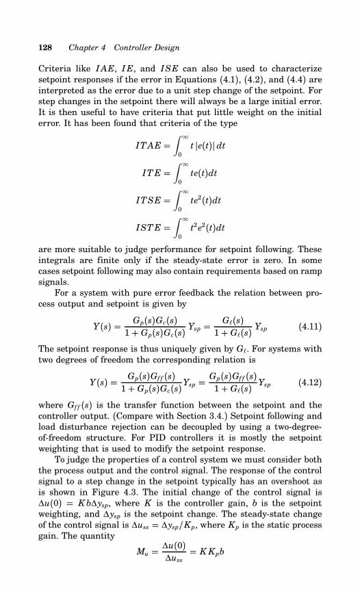
128 Chapter 4 Controller Design
Criteria like IAE, IE, and ISE can also be used to characterizesetpoint responses if the error in Equations (4.1), (4.2), and (4.4) areinterpreted as the error due to a unit step change of the setpoint. Forstep changes in the setpoint there will always be a large initial error.It is then useful to have criteria that put little weight on the initialerror. It has been found that criteria of the type
ITAE =∫ ∞
0t e(t) dt
ITE =∫ ∞
0te(t)dt
ITSE =∫ ∞
0te2(t)dt
ISTE =∫ ∞
0t2e2(t)dt
are more suitable to judge performance for setpoint following. Theseintegrals are finite only if the steady-state error is zero. In somecases setpoint following may also contain requirements based on rampsignals.For a system with pure error feedback the relation between pro-
cess output and setpoint is given by
Y(s) = Gp(s)Gc(s)1+ Gp(s)Gc(s) Ysp =
G(s)1+ G(s) Ysp (4.11)
The setpoint response is thus uniquely given by G. For systems withtwo degrees of freedom the corresponding relation is
Y(s) = Gp(s)Gf f (s)1+ Gp(s)Gc(s)Ysp =
Gp(s)Gf f (s)1+ G(s) Ysp (4.12)
where Gf f (s) is the transfer function between the setpoint and thecontroller output. (Compare with Section 3.4.) Setpoint following andload disturbance rejection can be decoupled by using a two-degree-of-freedom structure. For PID controllers it is mostly the setpointweighting that is used to modify the setpoint response.To judge the properties of a control system we must consider both
the process output and the control signal. The response of the controlsignal to a step change in the setpoint typically has an overshoot asis shown in Figure 4.3. The initial change of the control signal is∆u(0) = Kb∆ysp, where K is the controller gain, b is the setpointweighting, and ∆ysp is the setpoint change. The steady-state changeof the control signal is ∆uss = ∆ysp/Kp, where Kp is the static processgain. The quantity
Mu = ∆u(0)∆uss
= K Kpb
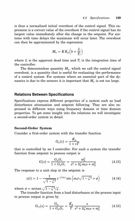
4.2 Specifications 129
is thus a normalized initial overshoot of the control signal. This ex-pression is a correct value of the overshoot if the control signal has itslargest value immediately after the change in the setpoint. For sys-tems with time delays the maximum will occur later. The overshootcan then be approximated by the expression
Mu = K Kp(b+ LTi
)where L is the apparent dead time and Ti is the integration time ofthe controller.The dimensionless quantity Mu, which we call the control signal
overshoot, is a quantity that is useful for evaluating the performanceof a control system. For systems where an essential part of the dy-namics is due to the sensors it is important that Mu is not too large.
Relations Between Specifications
Specifications express different properties of a system such as loaddisturbance attenuation and setpoint following. They are also ex-pressed in different ways using frequency domain or time domainproperties. To get some insight into the relations we will investigatea second-order system in detail.
Second-Order System
Consider a first-order system with the transfer function
Gp(s) = Kp
1+ sTthat is controlled by an I controller. For such a system the transferfunction from setpoint to process output is
G(s) = GpGc
1+ GpGc =ω 20
s2 + 2ζ ω 0s+ω 20(4.13)
The response to a unit step in the setpoint is
y(t) = 1− 1√1− ζ 2
e−ζ ω 0t sin(
ω 0t√1− ζ 2 + φ
)(4.14)
where φ = arctan√1− ζ 2/ζ .
The transfer function from a load disturbance at the process inputto process output is given by
Gly(s) = Gp
1+ GpGc =Kp
T
s
s2 + 2ζ ω 0s+ω 20(4.15)
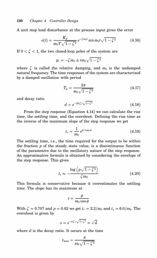
130 Chapter 4 Controller Design
A unit step load disturbance at the process input gives the error
e(t) = Kp
ω 0T√1− ζ 2
e−ζ ω 0t sinω 0t√1− ζ 2 (4.16)
If 0 < ζ < 1, the two closed-loop poles of the system are
pi = −ζ ω 0 ± iω 0√1− ζ 2
where ζ is called the relative damping, and ω 0 is the undampednatural frequency. The time responses of the system are characterizedby a damped oscillation with period
Tp = 2π
ω 0√1− ζ 2
(4.17)
and decay ratio
d = e−2πζ /√1−ζ 2 (4.18)
From the step response (Equation 4.14) we can calculate the risetime, the settling time, and the overshoot. Defining the rise time asthe inverse of the maximum slope of the step response we get
tr = 1ω 0eφ/ tanφ (4.19)
The settling time, i.e., the time required for the output to be withinthe fraction p of the steady state value, is a discontinuous functionof the parameters due to the oscillatory nature of the step response.An approximative formula is obtained by considering the envelope ofthe step response. This gives
ts −log
(p√1− ζ 2
)ζ ω 0
(4.20)
This formula is conservative because it overestimates the settlingtime. The slope has its maximum at
t = φ
ω 0 cosφ
With ζ = 0.707 and p = 0.02 we get tr = 2.2/ω 0 and ts = 6.0/ω 0. Theovershoot is given by
o = e−πζ /√1−ζ 2 =
√d
where d is the decay ratio. It occurs at the time
tmax = π
ω 0√1− ζ 2
4.2 Specifications 131
The overshoot is 4% for ζ = 0.707, 8% for ζ = 0.63, 16% for ζ = 0.5.It is 50% for quarter amplitude decay ratio.Equation (4.16) gives the error signal after a step disturbance at
the process input. This signal has the maximum
emax = Kp
ω 0T√1− ζ 2
e−φ tanφ sinφ
for
tmax = 1
ω 0√1− ζ 2
φ
The integrated error is
IE = Kp
ω 20T
This quantity is close to the IAE, if the overshoot is sufficiently small.The high-frequency gain of the controller is
Khf = 2ζ ω 0T − 1Kp
2ζ ω 0T
Kp
where the approximation holds when ω 0T is large. The sensitivity is
Ms =√1+ 8ζ 2 + (1+ 4ζ 2)
√1+ 8ζ 2
1+ 8ζ 2 + (−1+ 4ζ 2)√1+ 8ζ 2
The sensitivity function is infinite for ζ = 0 and decreases withincreasing ζ . Its values for ζ = 0.3, 0.5, and 0.7 are 2.0, 1.5, and1.3. To have a reasonable value of the sensitivity it must, therefore,be required that the relative damping is greater than 0.3. This impliesthat the decay ratio d must be smaller than 0.14.The equations given can be used to understand how the proper-
ties of the closed-loop system are influenced by ω 0 and ζ . The in-tegrated error is inversely proportional to ω−20 . The maximum error,the rise time, and the settling time are proportional to ω−10 . The high-frequency gain of the controller is proportional to ω 0. Both the loaddisturbance response and the setpoint response are improved by in-creasing ω 0. The control actions generated by noise do increase, how-ever, with ω 0. The overshoot, the decay ratio, and the sensitivity willincrease with decreasing ζ .This general pattern also holds for more complex systems. Both
load disturbance attenuation and response time to setpoint changeswill generally increase with increasing bandwidth of the system. Formore complex controllers, the load disturbance response and the set-point response can be specified separately.
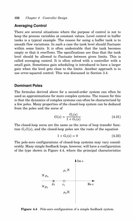
132 Chapter 4 Controller Design
Averaging Control
There are several situations where the purpose of control is not tokeep the process variables at constant values. Level control in buffertanks is a typical example. The reason for using a buffer tank is tosmooth flow variations. In such a case the tank level should fluctuatewithin some limits. It is often undesirable that the tank becomesempty or that it overflows. The specifications are thus that the tanklevel should be allowed to fluctuate between given limits. This iscalled averaging control. It is often solved with a controller with asmall gain. Sometimes gain scheduling is introduced to have a largergain when the level gets close to the limits. Another approach is touse error-squared control. This was discussed in Section 3.4.
Dominant Poles
The formulas derived above for a second-order system can often beused as approximations for more complex systems. The reason for thisis that the dynamics of complex systems can often be characterized bya few poles. Many properties of the closed-loop system can be deducedfrom the poles and the zeros of
G(s) = G(s)1+ G(s) (4.21)
The closed-loop zeros are the same as the zeros of loop transfer func-tion Gell(s), and the closed-loop poles are the roots of the equation
1+ G(s) = 0 (4.22)The pole-zero configurations of closed-loop systems may vary consid-erably. Many simple feedback loops, however, will have a configurationof the type shown in Figure 4.4, where the principal characteristics
Im s
Re s
z1
p2
p3
p5
p4
p1
Figure 4.4 Pole-zero configuration of a simple feedback system.
4.2 Specifications 133
of the response are given by a complex pair of poles, p1 and p2, calledthe dominant poles. The response is also influenced by real poles andzeros p3 and z1 close to the origin. The position of p3 and z1 may bereversed. There may also be more poles and zeros far from the origin,which typically are of less influence. Poles and zeros with real partsmuch smaller than the real part of the dominant poles have littleinfluence on the transient response.Complex poles are often characterized in terms of their frequency
ω 0, which is the distance from the origin, and their relative dampingζ . If a pair of complex poles is dominating, the formulas derived abovefor a second-order system can be used as approximation. Classicalcontrol was very much concerned with closed-loop systems havingthe pole-zero configuration shown in Figure 4.4.Even if many closed-loop systems have a pole-zero configuration
similar to the one shown in Figure 4.4, there are, however, exceptions.For instance, systems with mechanical resonances, which may havepoles and zeros close to the imaginary axis, are generic examples ofsystems that do not fit the pole-zero pattern of the figure. Anotherexample is processes with a long dead time.
Determination of the Dominant Poles from theFrequency Response
A simple method for approximate determination of the dominant polesfrom knowledge of the Nyquist curve of the loop transfer function willnow be given. Consider the loop transfer function G(s) as a mappingfrom the s-plane to the G-plane. The map of the imaginary axis inthe s-plane is the Nyquist curve G(iω ), which is indicated in Figure4.5.The closed-loop poles are the roots of the characteristic equation
1+ G(s) = 0The map of a straight vertical line through the dominant closed-looppoles in the s-plane is thus a curve through the critical point G = −1in the G-plane. This curve is shown by a dashed line in Figure4.5. Since the map is conform, the straight line A′C′ is mapped onthe curve AC, which intersects the Nyquist curve orthogonally. Thetriangle ABC is also mapped conformally to A′B′C′. If ABC can beapproximated by a triangle, we have
G(iω 2) − G(iω 1)iω 2 − iω 1 1+ G(iω 2)
σ
When ω 1 is close to ω 2 this becomes
σ = (1+ G(iω 2)) iω 2 − iω 1G(iω 2) − G(iω 1)
1+ G(iω 2)G ′(iω 2)
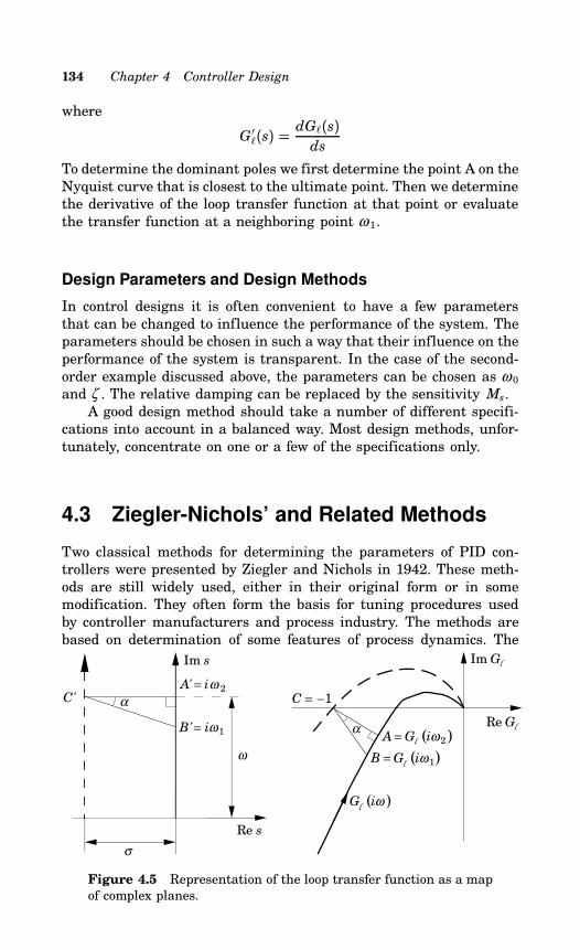
134 Chapter 4 Controller Design
where
G ′(s) =dG(s)ds
To determine the dominant poles we first determine the point A on theNyquist curve that is closest to the ultimate point. Then we determinethe derivative of the loop transfer function at that point or evaluatethe transfer function at a neighboring point ω 1.
Design Parameters and Design Methods
In control designs it is often convenient to have a few parametersthat can be changed to influence the performance of the system. Theparameters should be chosen in such a way that their influence on theperformance of the system is transparent. In the case of the second-order example discussed above, the parameters can be chosen as ω 0and ζ . The relative damping can be replaced by the sensitivity Ms.A good design method should take a number of different specifi-
cations into account in a balanced way. Most design methods, unfor-tunately, concentrate on one or a few of the specifications only.
4.3 Ziegler-Nichols’ and Related Methods
Two classical methods for determining the parameters of PID con-trollers were presented by Ziegler and Nichols in 1942. These meth-ods are still widely used, either in their original form or in somemodification. They often form the basis for tuning procedures usedby controller manufacturers and process industry. The methods arebased on determination of some features of process dynamics. The
C = −1
αRe G
Im G
A = G iω2( )
B = G iω1( )
G iω( )
l
l
l
l
l
Re s
Im s
B'= iω1
A' = iω 2C'
ω
α
σ
Figure 4.5 Representation of the loop transfer function as a mapof complex planes.
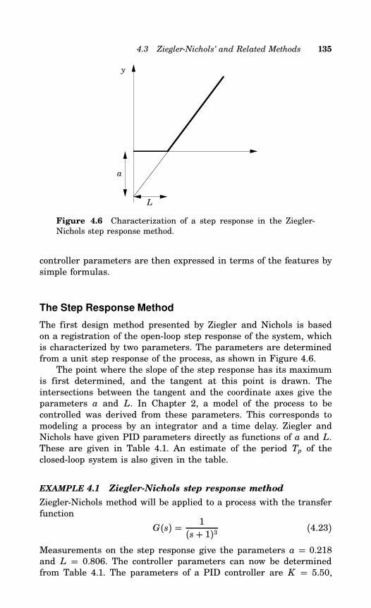
4.3 Ziegler-Nichols’ and Related Methods 135
a
L
y
Figure 4.6 Characterization of a step response in the Ziegler-Nichols step response method.
controller parameters are then expressed in terms of the features bysimple formulas.
The Step Response Method
The first design method presented by Ziegler and Nichols is basedon a registration of the open-loop step response of the system, whichis characterized by two parameters. The parameters are determinedfrom a unit step response of the process, as shown in Figure 4.6.The point where the slope of the step response has its maximum
is first determined, and the tangent at this point is drawn. Theintersections between the tangent and the coordinate axes give theparameters a and L. In Chapter 2, a model of the process to becontrolled was derived from these parameters. This corresponds tomodeling a process by an integrator and a time delay. Ziegler andNichols have given PID parameters directly as functions of a and L.These are given in Table 4.1. An estimate of the period Tp of theclosed-loop system is also given in the table.
EXAMPLE 4.1 Ziegler-Nichols step response method
Ziegler-Nichols method will be applied to a process with the transferfunction
G(s) = 1(s+ 1)3 (4.23)
Measurements on the step response give the parameters a = 0.218and L = 0.806. The controller parameters can now be determinedfrom Table 4.1. The parameters of a PID controller are K = 5.50,
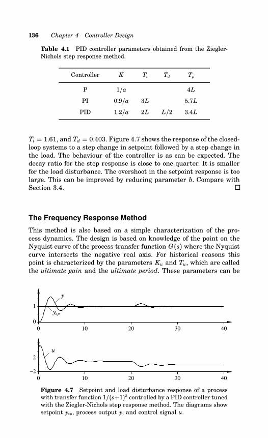
136 Chapter 4 Controller Design
Table 4.1 PID controller parameters obtained from the Ziegler-Nichols step response method.
Controller K Ti Td Tp
P 1/a 4L
PI 0.9/a 3L 5.7L
PID 1.2/a 2L L/2 3.4L
Ti = 1.61, and Td = 0.403. Figure 4.7 shows the response of the closed-loop systems to a step change in setpoint followed by a step change inthe load. The behaviour of the controller is as can be expected. Thedecay ratio for the step response is close to one quarter. It is smallerfor the load disturbance. The overshoot in the setpoint response is toolarge. This can be improved by reducing parameter b. Compare withSection 3.4.
The Frequency Response Method
This method is also based on a simple characterization of the pro-cess dynamics. The design is based on knowledge of the point on theNyquist curve of the process transfer function G(s) where the Nyquistcurve intersects the negative real axis. For historical reasons thispoint is characterized by the parameters Ku and Tu, which are calledthe ultimate gain and the ultimate period. These parameters can be
0 10 20 30 400
1
0 10 20 30 40−2
2
y
ysp
u
Figure 4.7 Setpoint and load disturbance response of a processwith transfer function 1/(s+1)3 controlled by a PID controller tunedwith the Ziegler-Nichols step response method. The diagrams showsetpoint ysp, process output y, and control signal u.
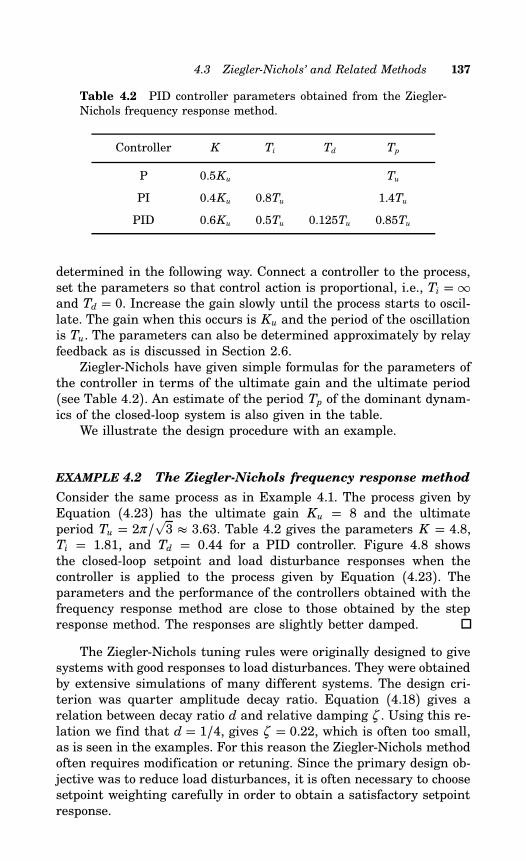
4.3 Ziegler-Nichols’ and Related Methods 137
Table 4.2 PID controller parameters obtained from the Ziegler-Nichols frequency response method.
Controller K Ti Td Tp
P 0.5Ku Tu
PI 0.4Ku 0.8Tu 1.4Tu
PID 0.6Ku 0.5Tu 0.125Tu 0.85Tu
determined in the following way. Connect a controller to the process,set the parameters so that control action is proportional, i.e., Ti = ∞and Td = 0. Increase the gain slowly until the process starts to oscil-late. The gain when this occurs is Ku and the period of the oscillationis Tu. The parameters can also be determined approximately by relayfeedback as is discussed in Section 2.6.Ziegler-Nichols have given simple formulas for the parameters of
the controller in terms of the ultimate gain and the ultimate period(see Table 4.2). An estimate of the period Tp of the dominant dynam-ics of the closed-loop system is also given in the table.We illustrate the design procedure with an example.
EXAMPLE 4.2 The Ziegler-Nichols frequency response method
Consider the same process as in Example 4.1. The process given byEquation (4.23) has the ultimate gain Ku = 8 and the ultimateperiod Tu = 2π/
√3 3.63. Table 4.2 gives the parameters K = 4.8,
Ti = 1.81, and Td = 0.44 for a PID controller. Figure 4.8 showsthe closed-loop setpoint and load disturbance responses when thecontroller is applied to the process given by Equation (4.23). Theparameters and the performance of the controllers obtained with thefrequency response method are close to those obtained by the stepresponse method. The responses are slightly better damped.
The Ziegler-Nichols tuning rules were originally designed to givesystems with good responses to load disturbances. They were obtainedby extensive simulations of many different systems. The design cri-terion was quarter amplitude decay ratio. Equation (4.18) gives arelation between decay ratio d and relative damping ζ . Using this re-lation we find that d = 1/4, gives ζ = 0.22, which is often too small,as is seen in the examples. For this reason the Ziegler-Nichols methodoften requires modification or retuning. Since the primary design ob-jective was to reduce load disturbances, it is often necessary to choosesetpoint weighting carefully in order to obtain a satisfactory setpointresponse.
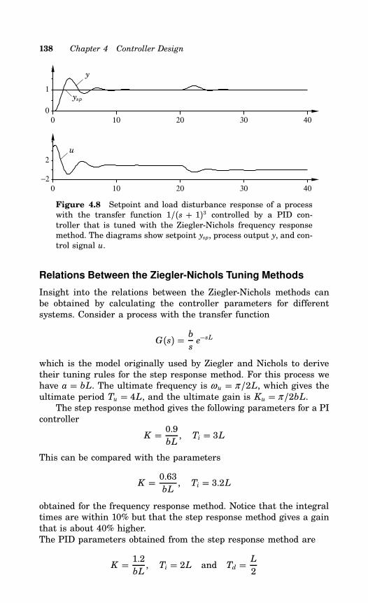
138 Chapter 4 Controller Design
0 10 20 30 400
1
0 10 20 30 40−2
2
y
ysp
u
Figure 4.8 Setpoint and load disturbance response of a processwith the transfer function 1/(s + 1)3 controlled by a PID con-troller that is tuned with the Ziegler-Nichols frequency responsemethod. The diagrams show setpoint ysp, process output y, and con-trol signal u.
Relations Between the Ziegler-Nichols Tuning Methods
Insight into the relations between the Ziegler-Nichols methods canbe obtained by calculating the controller parameters for differentsystems. Consider a process with the transfer function
G(s) = bse−sL
which is the model originally used by Ziegler and Nichols to derivetheir tuning rules for the step response method. For this process wehave a = bL. The ultimate frequency is ωu = π/2L, which gives theultimate period Tu = 4L, and the ultimate gain is Ku = π/2bL.The step response method gives the following parameters for a PI
controller
K = 0.9bL, Ti = 3L
This can be compared with the parameters
K = 0.63bL, Ti = 3.2L
obtained for the frequency response method. Notice that the integraltimes are within 10% but that the step response method gives a gainthat is about 40% higher.The PID parameters obtained from the step response method are
K = 1.2bL, Ti = 2L and Td = L2
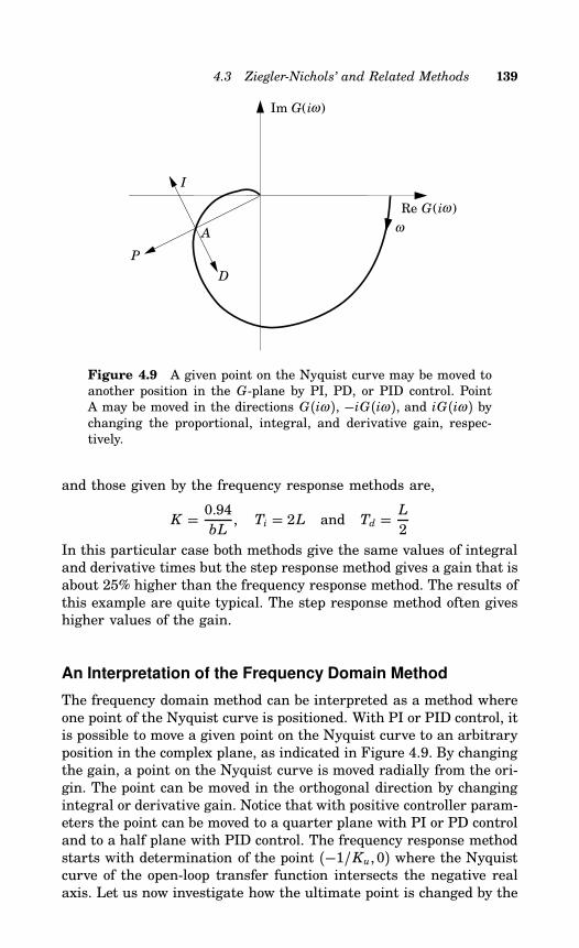
4.3 Ziegler-Nichols’ and Related Methods 139
Re G(iω )
Im G(iω )
ω
D
P
A
I
Figure 4.9 A given point on the Nyquist curve may be moved toanother position in the G-plane by PI, PD, or PID control. PointA may be moved in the directions G(iω ), −iG(iω ), and iG(iω ) bychanging the proportional, integral, and derivative gain, respec-tively.
and those given by the frequency response methods are,
K = 0.94bL, Ti = 2L and Td = L2
In this particular case both methods give the same values of integraland derivative times but the step response method gives a gain that isabout 25% higher than the frequency response method. The results ofthis example are quite typical. The step response method often giveshigher values of the gain.
An Interpretation of the Frequency Domain Method
The frequency domain method can be interpreted as a method whereone point of the Nyquist curve is positioned. With PI or PID control, itis possible to move a given point on the Nyquist curve to an arbitraryposition in the complex plane, as indicated in Figure 4.9. By changingthe gain, a point on the Nyquist curve is moved radially from the ori-gin. The point can be moved in the orthogonal direction by changingintegral or derivative gain. Notice that with positive controller param-eters the point can be moved to a quarter plane with PI or PD controland to a half plane with PID control. The frequency response methodstarts with determination of the point (−1/Ku, 0) where the Nyquistcurve of the open-loop transfer function intersects the negative realaxis. Let us now investigate how the ultimate point is changed by the
140 Chapter 4 Controller Design
controller. For a PI controller with Ziegler-Nichols tuning we haveK = 0.4Ku and ωuTi = (2π/Tu)0.8Tu = 5.02. Thererfore, the transferfunction of the PI controller at the ultimate frequency is
Gc(iωu) = K(1+ 1iωuTi
)= 0.4Ku(1− i/5.02) = Ku(0.4− 0.08i)
The ultimate point is thus moved to −0.4+ 0.08i. This means that alag of 11.2 is introduced at the ultimate frequency.For a PID controller we have K = 0.6Ku, ωuTi = π and ωuTd =
π/4. The frequency response of the controller at frequency ωu is
Gc(iωu) = K(1+ i
(ωuTd − 1
ωuTi
))= 0.6Ku
(1+ i
(π
4− 1
π
))
0.6Ku(1+ 0.467i)This controller gives a phase advance of 25 at the ultimate frequency.The loop transfer function is
G(iωu) = Gp(iωu)Gc(iωu) = −0.6(1+ 0.467i) = −0.6− 0.28iThe Ziegler-Nichols frequency response method thus moves the ulti-mate point (−1/Ku, 0) to the point −0.6 − 0.28i. The distance fromthis point to the critical point is 0.5. This means that the methodgives a sensitivity that is always greater than 2.
Modified Ziegler-Nichols Method
With the given interpretation of the frequency domain method, it isstraightforward to generalize it in the following way. Choose an arbi-trary point on the Nyquist curve of the open-loop system. Determine acontroller that moves this point to a suitable location. Let the chosenpoint be
A = Gp(iω 0) = raei(π+φa)
Determine a controller that moves this point to
B = G(iω 0) = rbei(π+φb)
Writing the frequency response of the controller as Gc(iω 0) = rceiφ cwe get
rbei(π+φb) = rarcei(π+φa+φ c)
The controller should thus be chosen so that
rc = rbra
φ c = φb − φa
4.3 Ziegler-Nichols’ and Related Methods 141
For a PI controller this implies
K = rb cos (φb − φa)ra
Ti = 1ω 0 tan (φa − φb)
(4.24)
This means that we must require φa > φb in order to have positiveTi. For a PID controller we get similarly
K = rb cos (φb − φa)ra
ω 0Td − 1ω 0Ti
= tan (φb − φa)(4.25)
The gain K is uniquely given. There is, however, only one equation todetermine parameters Ti and Td. An additional condition must thusbe introduced to determine these parameters uniquely. A commonmethod is to specify that the ratio of these parameters is constant,i.e.,
Td = αTi
as in the Ziegler-Nichols rules, where α = 0.25. Straightforwardcalculations then give
Ti = 12αω 0
(tan (φb − φa) +
√4α + tan2 (φb − φa)
)Td = αTi
(4.26)
Assuming that a Ziegler-Nichols experiment is used to determine asuitable point, we have ra = 1/Ku and φa = 0. The PI controllerparameters then become
K = Kurb cosφb
Ti = − Tu
2π tanφb
(4.27)
Notice that φb must be negative in order to have positive controllerparameters. Choosing α = 0.25, the PID controller parameters aregiven by
K = Kurb cosφb
Ti = Tuπ
(1+ sinφbcosφb
)Td = Tu4π
(1+ sinφbcosφb
) (4.28)
Notice that the tuning rules are of the same form as for the frequencyresponse method but with different values of the numerical parame-ters. Systems with better damping than the Ziegler-Nichols rules can
142 Chapter 4 Controller Design
be obtained by proper choices of rb and φb. A reasonable choice isrb = 0.5 and φb = 20.It has been suggested by Pessen to move the ultimate point to
−0.2 − 0.36i or −0.2 − 0.21i. This corresponds to rb = 0.41 andφb = 61, and rb = 0.29 and φb = 46 respectively.There are limitations with a design method where only one point
on the Nyquist curve is positioned. The properties of the closed-loopsystem can then change significantly depending on the slope of thecurve. This is illustrated in Figure 4.10, which shows the Nyquistcurves of three systems having the same amplitude margin, Am = 2,which means that the Nyquist curves of all systems pass through thepoint (−0.5, 0). The figure also shows the closed-loop responses to astep change in setpoint.
Assessment of Ziegler-Nichols Tuning
The Ziegler-Nichols tuning procedures are simple and intuitive. Theyrequire little process knowledge and they can be applied with modesteffort. These are some of the reasons why they are so widely used.The methods have, however, some limitations as we have alreadyseen. A fundamental drawback is that the basic design criterion isto obtain a closed-loop system with quarter amplitude decay ratio(d = 0.25). This gives good rejection of load disturbances, but alsocreates a closed-loop system that is very poorly damped and that haspoor stability margins. The closed-loop gain is typically 2 to 3 timestoo high. The frequency response method is more reliable than thestep response method. One reason for this is that the ultimate gain isuniquely defined, but that there are many ways to define the apparentdead time. The step response method typically also gives somewhathigher gains.The methods generally will work better for PID control than for
PI control. The reason for this will be discussed in Chapter 5. Let itsuffice here to give an example.
EXAMPLE 4.3 PI control
Consider the same process as in Examples 4.1 and 4.2, where thetransfer function has three equal lags. See Equation (4.23). Mea-surements on the step response give the parameters a = 0.218 andL = 0.806. The step response method gives a PI controller with pa-rameters K = 4.13 and Ti = 2.42. The ultimate gain is Ku = 8 andthe ultimate period is Tu = 2π/
√3 3.63. The frequency domain
method gives a PI controller with parameters K = 3.2 and Ti = 2.90.Notice that the gains obtained with the frequency response methodare lower than those obtained with the step response method. Figure
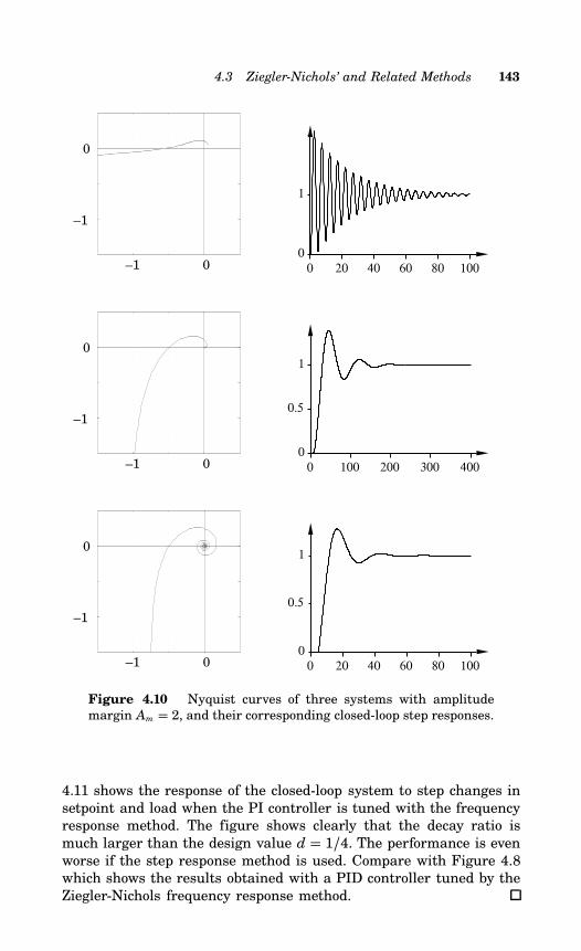
4.3 Ziegler-Nichols’ and Related Methods 143
0 20 40 60 80 1000
1
–1 0
–1
0
0 100 200 300 4000
0.5
1
–1 0
–1
0
0 20 40 60 80 1000
0.5
1
–1 0
–1
0
Figure 4.10 Nyquist curves of three systems with amplitudemargin Am = 2, and their corresponding closed-loop step responses.
4.11 shows the response of the closed-loop system to step changes insetpoint and load when the PI controller is tuned with the frequencyresponse method. The figure shows clearly that the decay ratio ismuch larger than the design value d = 1/4. The performance is evenworse if the step response method is used. Compare with Figure 4.8which shows the results obtained with a PID controller tuned by theZiegler-Nichols frequency response method.
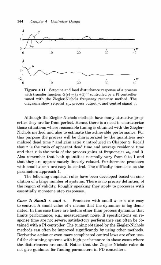
144 Chapter 4 Controller Design
0 10 20 30 400
1
0 10 20 30 40−2
2
y
ysp
u
Figure 4.11 Setpoint and load disturbance response of a processwith transfer function G(s) = (s+1)−3 controlled by a PI controllertuned with the Ziegler-Nichols frequency response method. Thediagrams show setpoint ysp, process output y, and control signal u.
Although the Ziegler-Nichols methods have many attractive prop-erties they are far from perfect. Hence, there is a need to characterizethose situations where reasonable tuning is obtained with the Ziegler-Nichols method and also to estimate the achievable performance. Forthis purpose the process will be characterized by the quantities nor-malized dead time τ and gain ratio κ introduced in Chapter 2. Recallthat τ is the ratio of apparent dead time and average residence timeand that κ is the ratio of the process gains at frequencies ωu and 0.Also remember that both quantities normally vary from 0 to 1 andthat they are approximately linearly related. Furthermore processeswith small κ or τ are easy to control. The difficulty increases as theparameters approach 1.The following empirical rules have been developed based on sim-
ulation of a large number of systems. There is no precise definition ofthe region of validity. Roughly speaking they apply to processes withessentially monotone step responses.
Case 1: Small κ and τ . Processes with small κ or τ are easyto control. A small value of τ means that the dynamics is lag domi-nated. In this case there are factors other than process dynamics thatlimits performance, e.g., measurement noise. If specifications on re-sponse time are not severe, satisfactory performance can often be ob-tained with a PI controller. The tuning obtained by the Ziegler-Nicholsmethods can often be improved significantly by using other methods.Derivative action or even more complicated control laws are often use-ful for obtaining systems with high performance in those cases wherethe disturbances are small. Notice that the Ziegler-Nichols rules donot give guidance for finding parameters in PD controllers.
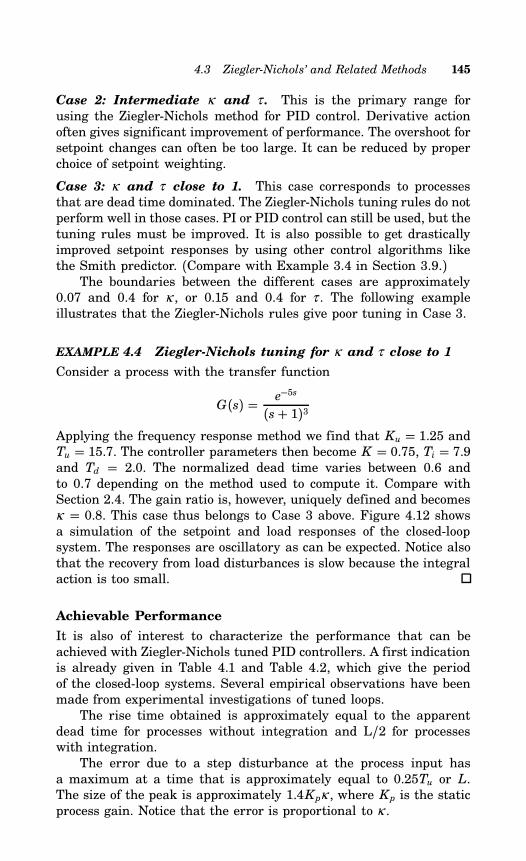
4.3 Ziegler-Nichols’ and Related Methods 145
Case 2: Intermediate κ and τ . This is the primary range forusing the Ziegler-Nichols method for PID control. Derivative actionoften gives significant improvement of performance. The overshoot forsetpoint changes can often be too large. It can be reduced by properchoice of setpoint weighting.
Case 3: κ and τ close to 1. This case corresponds to processesthat are dead time dominated. The Ziegler-Nichols tuning rules do notperform well in those cases. PI or PID control can still be used, but thetuning rules must be improved. It is also possible to get drasticallyimproved setpoint responses by using other control algorithms likethe Smith predictor. (Compare with Example 3.4 in Section 3.9.)The boundaries between the different cases are approximately
0.07 and 0.4 for κ , or 0.15 and 0.4 for τ . The following exampleillustrates that the Ziegler-Nichols rules give poor tuning in Case 3.
EXAMPLE 4.4 Ziegler-Nichols tuning for κ and τ close to 1
Consider a process with the transfer function
G(s) = e−5s
(s+ 1)3Applying the frequency response method we find that Ku = 1.25 andTu = 15.7. The controller parameters then become K = 0.75, Ti = 7.9and Td = 2.0. The normalized dead time varies between 0.6 andto 0.7 depending on the method used to compute it. Compare withSection 2.4. The gain ratio is, however, uniquely defined and becomesκ = 0.8. This case thus belongs to Case 3 above. Figure 4.12 showsa simulation of the setpoint and load responses of the closed-loopsystem. The responses are oscillatory as can be expected. Notice alsothat the recovery from load disturbances is slow because the integralaction is too small.
Achievable Performance
It is also of interest to characterize the performance that can beachieved with Ziegler-Nichols tuned PID controllers. A first indicationis already given in Table 4.1 and Table 4.2, which give the periodof the closed-loop systems. Several empirical observations have beenmade from experimental investigations of tuned loops.The rise time obtained is approximately equal to the apparent
dead time for processes without integration and L/2 for processeswith integration.The error due to a step disturbance at the process input has
a maximum at a time that is approximately equal to 0.25Tu or L.The size of the peak is approximately 1.4Kpκ , where Kp is the staticprocess gain. Notice that the error is proportional to κ .
146 Chapter 4 Controller Design
0 50 100 1500
1
0 50 100 150−1
1
ysp
y
u
Figure 4.12 Step responses of a process with the transfer func-tion G(s) = e−5s/(s + 1)3 controlled by PID controllers tuned withthe Ziegler-Nichols frequency response method. The diagrams showsetpoint ysp, process output y, and control signal u.
With Ziegler-Nichols tuning the sensitivity is always larger than2. In Section 4.2 it was shown that a quarter amplitude decay ratiocorresponds to a sensitivity Ms = 2.6.
Tuning Maps
Since the Ziegler-Nichols methods only give “ball-park” values, it isnecessary to make manual tuning to obtain the desired performance.A device called tuning maps have been developed to guide man-ual tuning. The purpose of these maps is to provide intuition abouthow changes in controller parameters influence the behaviour of theclosed-loop system. The tuning maps are simply two-dimensional ar-rays of transient responses or frequency responses organized in asystematic way.An example of a tuning map is given in Figure 4.13. The figure
illustrates how the load disturbance response is influenced by changesin gain and integral time. The process model
G(s) = 1(s+ 1)8
has been used in the example. The Ziegler-Nichols frequency responsemethod gives the controller parameters K = 1.13, Ti = 7.58, andTd = 1.9. The figure shows clearly the benefits of having a smallervalue of Ti. Judging from the figure, the values K = 1 and Ti = 5.0appear reasonable. The figure also shows that the choice of Ti isfairly critical. Also notice that controllers with Ti < 7.6 cannot beimplemented on series form (compare with Section 3.4).
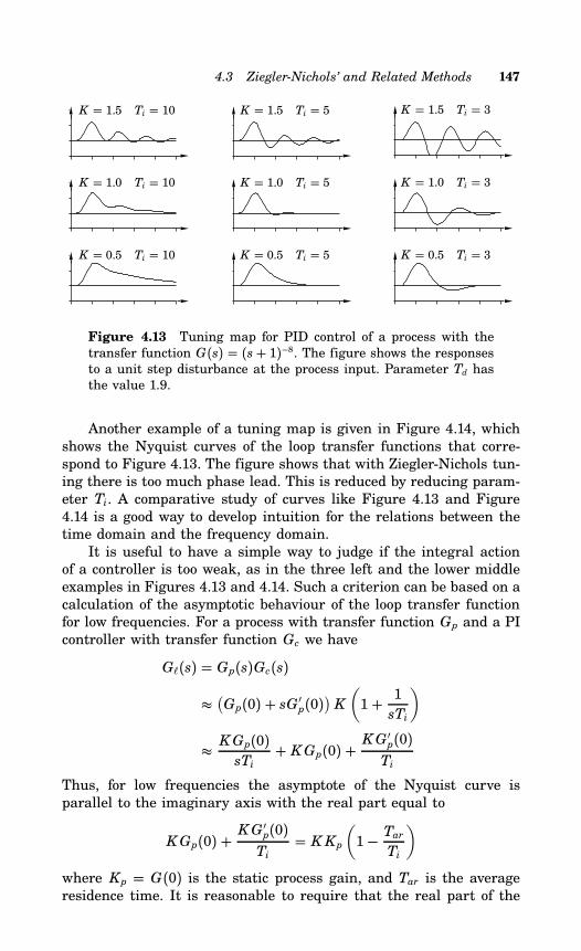
4.3 Ziegler-Nichols’ and Related Methods 147
K = 1.5 Ti = 10
K = 1.0 Ti = 10
K = 0.5 Ti = 10
K = 1.5 Ti = 5
K = 1.0 Ti = 5
K = 0.5 Ti = 5
K = 1.5 Ti = 3
K = 1.0 Ti = 3
K = 0.5 Ti = 3
Figure 4.13 Tuning map for PID control of a process with thetransfer function G(s) = (s+ 1)−8. The figure shows the responsesto a unit step disturbance at the process input. Parameter Td hasthe value 1.9.
Another example of a tuning map is given in Figure 4.14, whichshows the Nyquist curves of the loop transfer functions that corre-spond to Figure 4.13. The figure shows that with Ziegler-Nichols tun-ing there is too much phase lead. This is reduced by reducing param-eter Ti. A comparative study of curves like Figure 4.13 and Figure4.14 is a good way to develop intuition for the relations between thetime domain and the frequency domain.It is useful to have a simple way to judge if the integral action
of a controller is too weak, as in the three left and the lower middleexamples in Figures 4.13 and 4.14. Such a criterion can be based on acalculation of the asymptotic behaviour of the loop transfer functionfor low frequencies. For a process with transfer function Gp and a PIcontroller with transfer function Gc we have
G(s) = Gp(s)Gc(s)
(Gp(0) + sG ′p(0)
)K
(1+ 1sTi
)
KGp(0)sTi
+ KGp(0) +KG ′p(0)Ti
Thus, for low frequencies the asymptote of the Nyquist curve isparallel to the imaginary axis with the real part equal to
KGp(0) +KG ′p(0)Ti
= K Kp(1− Tar
Ti
)
where Kp = G(0) is the static process gain, and Tar is the averageresidence time. It is reasonable to require that the real part of the
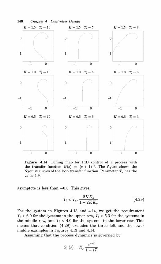
148 Chapter 4 Controller Design
x
x
K = 1.5 Ti = 10
–1 0
0
–1
x
x
K = 1.5 Ti = 5
–1 0
0
–1
x
x
K = 1.5 Ti = 3
–1 0
0
–1
x
x
x
K = 1.0 Ti = 10
–1 0
0
–1
x
x
K = 1.0 Ti = 5
–1 0
0
–1
x
x
K = 1.0 Ti = 3
–1 0
0
–1
x
x
x
K = 0.5 Ti = 10
–1 0
0
–1 x
x
x
K = 0.5 Ti = 5
–1 0
0
–1
x
x
x
K = 0.5 Ti = 3
–1 0
0
–1
Figure 4.14 Tuning map for PID control of a process withthe transfer function G(s) = (s + 1)−8. The figure shows theNyquist curves of the loop transfer function. Parameter Td has thevalue 1.9.
asymptote is less than −0.5. This gives
Ti < Tar 2K Kp1+ 2K Kp (4.29)
For the system in Figures 4.13 and 4.14, we get the requirementTi < 6.0 for the systems in the upper row, Ti < 5.3 for the systems inthe middle row, and Ti < 4.0 for the systems in the lower row. Thismeans that condition (4.29) excludes the three left and the lowermiddle examples in Figures 4.13 and 4.14.Assuming that the process dynamics is governed by
Gp(s) = Kp e−sL
1+ sT
4.3 Ziegler-Nichols’ and Related Methods 149
we find that Tar = L + T . With Ziegler-Nichols tuning of a PI con-troller, we then find that condition (4.29) is satisfied if
3L < (L + T) 1.8TL + 1.8T
This means that we must require that the normalized dead timesatisfies
τ = L
L+ T < 0.28
A similar calculation for a process described by
Gp(s) = Kp e−sL
(1+ sT)2which has
τ = L + (3− e)TL + 2T
shows that condition (4.29) holds for a PI controller tuned accordingto the Ziegler-Nichols method if
τ < 0.38We can thus conclude that the Ziegler-Nichols tuning rules for PI con-trollers can be applied only for small values of τ . The upper bound isapproximately τ = 0.3. For larger normalized dead times the integralaction is too weak.
The Chien, Hrones and Reswick Method
There has been many suggestions of modifications of the Ziegler-Nichols methods. Chien, Hrones and Reswick (CHR) changed thestep response method to give better damped closed-loop systems. Theyproposed to use “quickest response without overshoot” or “quickestresponse with 20% overshoot” as design criteria. They also madethe important observation that tuning for setpoint response or loaddisturbance response are different.To tune the controller according to the CHR method, the param-
eters a and L of the process model are first determined in the sameway as for the Ziegler-Nichols step response method. The controllerparameters for the load disturbance response method are then givenas functions of these two parameters. They are summarized in Ta-ble 4.3.The tuning rules based on the 20% overshoot design criteria in Ta-
ble 4.3 are quite similar to the Ziegler-Nichols step response methodpresented in Table 4.1. However, when the 0% overshoot design cri-teria is used, the gain and the derivative time are smaller and the
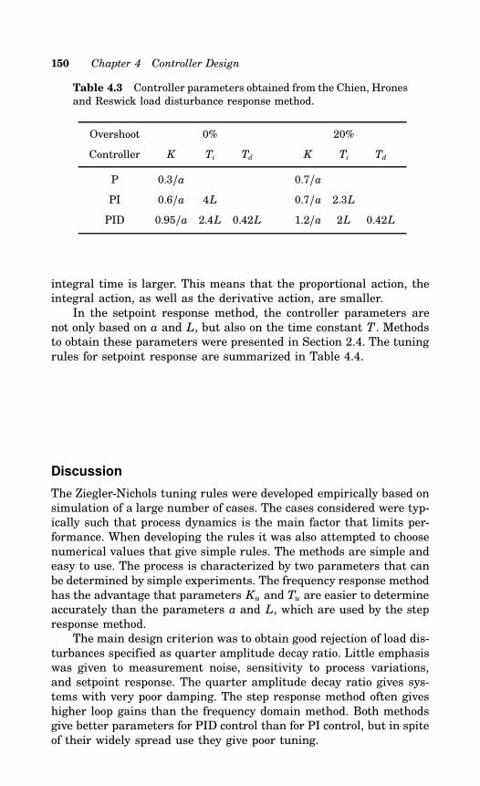
150 Chapter 4 Controller Design
Table 4.3 Controller parameters obtained from the Chien, Hronesand Reswick load disturbance response method.
Overshoot 0% 20%
Controller K Ti Td K Ti Td
P 0.3/a 0.7/aPI 0.6/a 4L 0.7/a 2.3L
PID 0.95/a 2.4L 0.42L 1.2/a 2L 0.42L
integral time is larger. This means that the proportional action, theintegral action, as well as the derivative action, are smaller.In the setpoint response method, the controller parameters are
not only based on a and L, but also on the time constant T . Methodsto obtain these parameters were presented in Section 2.4. The tuningrules for setpoint response are summarized in Table 4.4.
Discussion
The Ziegler-Nichols tuning rules were developed empirically based onsimulation of a large number of cases. The cases considered were typ-ically such that process dynamics is the main factor that limits per-formance. When developing the rules it was also attempted to choosenumerical values that give simple rules. The methods are simple andeasy to use. The process is characterized by two parameters that canbe determined by simple experiments. The frequency response methodhas the advantage that parameters Ku and Tu are easier to determineaccurately than the parameters a and L, which are used by the stepresponse method.The main design criterion was to obtain good rejection of load dis-
turbances specified as quarter amplitude decay ratio. Little emphasiswas given to measurement noise, sensitivity to process variations,and setpoint response. The quarter amplitude decay ratio gives sys-tems with very poor damping. The step response method often giveshigher loop gains than the frequency domain method. Both methodsgive better parameters for PID control than for PI control, but in spiteof their widely spread use they give poor tuning.
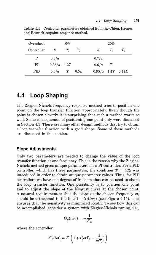
4.4 Loop Shaping 151
Table 4.4 Controller parameters obtained from the Chien, Hronesand Reswick setpoint response method.
Overshoot 0% 20%
Controller K Ti Td K Ti Td
P 0.3/a 0.7/aPI 0.35/a 1.2T 0.6/a T
PID 0.6/a T 0.5L 0.95/a 1.4T 0.47L
4.4 Loop Shaping
The Ziegler Nichols frequency response method tries to position onepoint on the loop transfer function appropriately. Even though thepoint is chosen cleverly it is surprising that such a method works sowell. Some consequences of positioning one point only were discussedin Section 4.3. There are many other design methods that try to obtaina loop transfer function with a good shape. Some of these methodsare discussed in this section.
Slope Adjustments
Only two parameters are needed to change the value of the looptransfer function at one frequency. This is the reason why the Ziegler-Nichols method gives unique parameters for a PI controller. For a PIDcontroller, which has three parameters, the condition Ti = 4Td wasintroduced in order to obtain unique parameter values. Thus, for PIDcontrollers we have one degree of freedom that can be used to shapethe loop transfer function. One possibility is to position one pointand to adjust the slope of the Nyquist curve at the chosen point.A natural requirement is that the slope at the chosen frequency ω 0should be orthogonal to the line 1 + G(iω 0) (see Figure 4.15). Thisensures that the sensitivity is minimized locally. To see how this canbe accomplished, consider a system with Ziegler-Nichols tuning, i.e.,
Gp(iωu) = − 1Ku
where the controller
Gc(iω ) = K(1+ i(ωTd − 1
ωTi
))
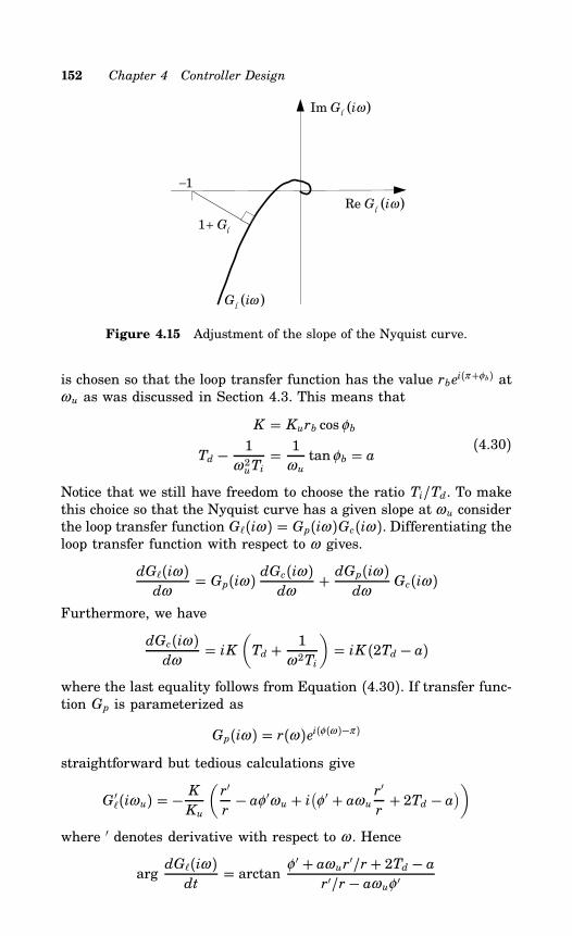
152 Chapter 4 Controller Design
−1
G iω( )
Re G iω( )
Im G iω( )
1+ Gl
l
l
l
Figure 4.15 Adjustment of the slope of the Nyquist curve.
is chosen so that the loop transfer function has the value rbei(π+φb) atωu as was discussed in Section 4.3. This means that
K = Kurb cosφb
Td − 1ω 2uTi
= 1ωutanφb = a
(4.30)
Notice that we still have freedom to choose the ratio Ti/Td. To makethis choice so that the Nyquist curve has a given slope at ωu considerthe loop transfer function G(iω ) = Gp(iω )Gc(iω ). Differentiating theloop transfer function with respect to ω gives.
dG(iω )dω
= Gp(iω ) dGc(iω )dω
+ dGp(iω )dω
Gc(iω )
Furthermore, we have
dGc(iω )dω
= iK(Td + 1
ω 2Ti
)= iK (2Td − a)
where the last equality follows from Equation (4.30). If transfer func-tion Gp is parameterized as
Gp(iω ) = r(ω )ei(φ(ω )−π )
straightforward but tedious calculations give
G ′(iωu) = −K
Ku
(r′
r− aφ ′ωu + i
(φ ′ + aωu r
′
r+ 2Td − a
))
where ′ denotes derivative with respect to ω . Hence
argdG(iω )dt
= arctan φ ′ + aωur′/r + 2Td − ar′/r − aωuφ ′
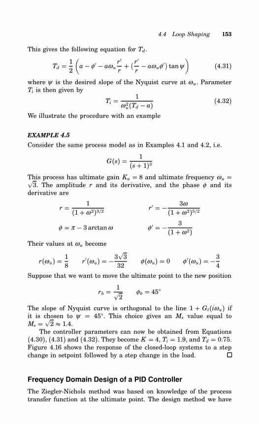
4.4 Loop Shaping 153
This gives the following equation for Td.
Td = 12(a− φ ′ − aωu r
′
r+ ( r′r− aωuφ ′
)tanψ
)(4.31)
where ψ is the desired slope of the Nyquist curve at ωu. ParameterTi is then given by
Ti = 1ω 2u(Td − a)
(4.32)
We illustrate the procedure with an example
EXAMPLE 4.5
Consider the same process model as in Examples 4.1 and 4.2, i.e.
G(s) = 1(s+ 1)3
This process has ultimate gain Ku = 8 and ultimate frequency ωu =√3. The amplitude r and its derivative, and the phase φ and itsderivative are
r = 1(1+ω 2)3/2 r′ = − 3ω
(1+ω 2)5/2
φ = π − 3 arctanω φ ′ = − 3(1+ω 2)
Their values at ωu become
r(ωu) = 18 r′(ωu) = −3√332
φ(ωu) = 0 φ ′(ωu) = −34Suppose that we want to move the ultimate point to the new position
rb = 1√2
φb = 45
The slope of Nyquist curve is orthogonal to the line 1 + G(iωu) ifit is chosen to ψ = 45. This choice gives an Ms value equal toMs =
√2 1.4.
The controller parameters can now be obtained from Equations(4.30), (4.31) and (4.32). They become K = 4, Ti = 1.9, and Td = 0.75.Figure 4.16 shows the response of the closed-loop systems to a stepchange in setpoint followed by a step change in the load.
Frequency Domain Design of a PID Controller
The Ziegler-Nichols method was based on knowledge of the processtransfer function at the ultimate point. The design method we have
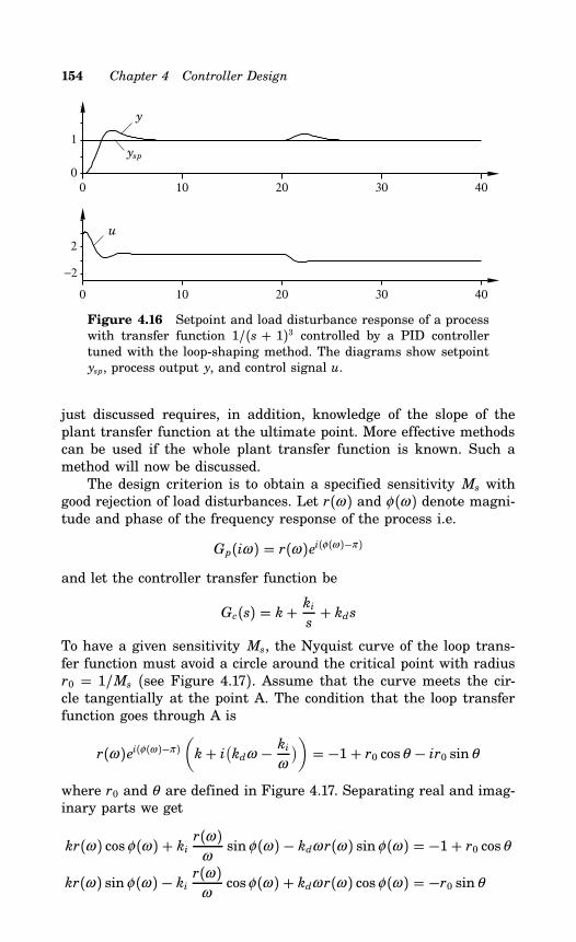
154 Chapter 4 Controller Design
0 10 20 30 400
1
0 10 20 30 40
−2
2
y
ysp
u
Figure 4.16 Setpoint and load disturbance response of a processwith transfer function 1/(s + 1)3 controlled by a PID controllertuned with the loop-shaping method. The diagrams show setpointysp, process output y, and control signal u.
just discussed requires, in addition, knowledge of the slope of theplant transfer function at the ultimate point. More effective methodscan be used if the whole plant transfer function is known. Such amethod will now be discussed.The design criterion is to obtain a specified sensitivity Ms with
good rejection of load disturbances. Let r(ω ) and φ(ω ) denote magni-tude and phase of the frequency response of the process i.e.
Gp(iω ) = r(ω )ei(φ(ω )−π )
and let the controller transfer function be
Gc(s) = k+ kis+ kds
To have a given sensitivity Ms, the Nyquist curve of the loop trans-fer function must avoid a circle around the critical point with radiusr0 = 1/Ms (see Figure 4.17). Assume that the curve meets the cir-cle tangentially at the point A. The condition that the loop transferfunction goes through A is
r(ω )ei(φ(ω )−π )(k+ i(kdω − ki
ω
)) = −1+ r0 cosθ − ir0 sinθ
where r0 and θ are defined in Figure 4.17. Separating real and imag-inary parts we get
kr(ω ) cosφ(ω ) + ki r(ω )ωsinφ(ω ) − kdω r(ω ) sinφ(ω ) = −1+ r0 cosθ
kr(ω ) sinφ(ω ) − ki r(ω )ωcosφ(ω ) + kdω r(ω ) cosφ(ω ) = −r0 sinθ
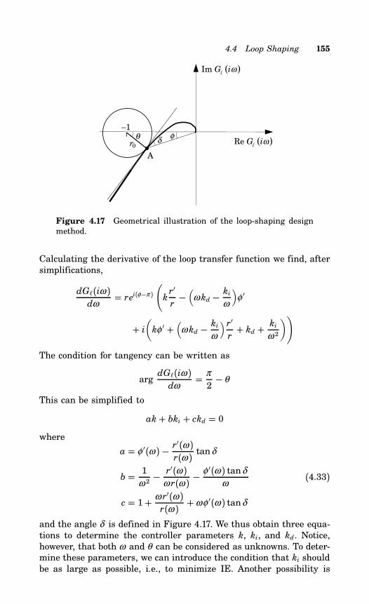
4.4 Loop Shaping 155
−1θ
A r0
δφ
Im G iω( )
Re G iω( )l
l
Figure 4.17 Geometrical illustration of the loop-shaping designmethod.
Calculating the derivative of the loop transfer function we find, aftersimplifications,
dG(iω )dω
= rei(φ−π )(kr′
r−
(ω kd − ki
ω
)φ ′
+ i(kφ ′ +
(ω kd − ki
ω
) r′r+ kd + ki
ω 2
))
The condition for tangency can be written as
argdG(iω )dω
= π
2− θ
This can be simplified to
ak+ bki + ckd = 0where
a = φ ′(ω ) − r′(ω )r(ω ) tanδ
b = 1ω 2− r
′(ω )ω r(ω ) −
φ ′(ω ) tanδ
ω
c = 1+ ω r′(ω )r(ω ) +ωφ ′(ω ) tanδ
(4.33)
and the angle δ is defined in Figure 4.17. We thus obtain three equa-tions to determine the controller parameters k, ki, and kd. Notice,however, that both ω and θ can be considered as unknowns. To deter-mine these parameters, we can introduce the condition that ki shouldbe as large as possible, i.e., to minimize IE. Another possibility is
156 Chapter 4 Controller Design
to make ω as large as possible. The design of the controller then isreduced to an optimization problem. Notice that parameter θ variesin the range (0,π/2). The value ωu can be used as an initial valuefor the optimization. Instead of minimizing IE we could also considerminimization of IAE. However, this will increase the computationaleffort considerably. Notice that when performing the optimization wealso obtain the argument ω 0 for which the optimum is achieved. Thisindicates the frequency range where model precision is needed.
4.5 Analytical Tuning Methods
There are several analytical tuning methods where the controllertransfer function is obtained from the specifications by a direct cal-culation. Let Gp and Gc be the transfer functions of the process andthe controller. The closed-loop transfer function obtained with errorfeedback is then
G0 = GpGc
1+ GpGcSolving this equation for Gc we get
Gc = 1Gp
⋅G0
1− G0 (4.34)
If the closed-loop transfer function G0 is specified and Gp is known, itis thus easy to compute Gc. The key problem is to find reasonable waysto determine G0 based on engineering specifications of the system.It follows from Equation (4.34) that all process poles and zeros
are canceled by the controller. This means that the method cannotbe applied when the process has poorly damped poles and zeros. Themethod will also give a poor load disturbance response when slowprocess poles are canceled.
λ-Tuning
The method called λ-tuning was developed for processes with longdead time L. Consider a process with the transfer function
Gp = Kp
1+ sT e−sL
Assume that the desired closed-loop transfer function is specified as
G0 = e−sL
1+ sλT
4.5 Analytical Tuning Methods 157
where λ is a tuning parameter. The time constants of the open- andclosed-loop systems are the same when λ = 1. The closed-loop systemresponds faster than the open-loop system if λ < 1. It is slower whenλ > 1.It follows from Equation (4.34) that the controller transfer func-
tion becomes
Gc = 1+ sTKp(1+ λsT − e−sL) (4.35)
The controller has integral action, because Gc(0) = ∞. The input-output relation of the controller is
(1+ sλT − e−sL)U (s) = 1
Kp(1+ sT)E(s) (4.36)
This can be written as
U (s) = 1λKp
(1+ 1sT
) (E(s) − Kp
1+ sT(1− e−sL)U (s)) (4.37)
When L = 0, this becomes a PI controller with gain K = 1/(λKp)and integral time Ti = T . The term
Kp
1+ sT(1− e−sL)U (s)
can be interpreted as a prediction of the process output at time tbased on the values of the control signal in the time interval (t−T , t).The controller given by Equation (4.37) can thus be interpreted as apredictive PI controller where the prediction is formed by correctingfor the effects of the control actions that have been taken, but have notyet appeared in the output because of the delay in the process. Thecontroller is, therefore, called a predictive PI controller (PPI). Forprocesses with long dead times, the prediction given in Equations(4.36) and (4.37) is much better than the prediction obtained byderivative action.The PPI controller can be written as
U (s) = 1λKp
(1+ 1sT
)E(s) − 1
sλT
(1− e−sL)U (s) (4.38)
In Section 4.2, it was shown that the integral error for a PIDcontroller is
IEPID = TiK
The integrated errors obtained with a PID controller and a controllerwith λ-tuning are compared. With a PID controller based on theZiegler-Nichols step response method, we obtain
IEPID = KpL2
0.6T
158 Chapter 4 Controller Design
To compute the integral error for the PPI controller it will be assumedthat the system is initially at rest and that a load disturbance in theform of a unit step is applied to the process input. Since the controllerhas integral action, we have u(∞) = 1. To integrate Equation (4.38),first note that
1λT
∫ ∞
0
(u(t) − u(t − L))dt = L
λT
Integration of Equation (4.38) from 0 to ∞ now gives
u(∞) − u(0) = 1 = 1λKpT
∫ ∞
0e(t)dt− L
λT
The integral error thus becomes
IEPPI = Kp(L + λT)The integrated error is smaller with PPI control than with PID
control when L is large. For λ = 1 the criteria are equal when L/T =1.1. The improvements with PPI control increases with decreasingvalues of λ .The sensitivity function obtained with λ-tuning is given by
S(s) = 1− e−sL
1+ sλT =1+ sλT − e−sL1+ sλT
It can be shown thatMs = max
ωS(iω )
is always less than 2. An approximate expression for Ms is given by
Ms = 2− λT
L
Thus, to have a value of Ms smaller than 2 it is important that λ issufficiently large.We note that in order to make the integrated error small it is
advantageous to have a small value of λ . A small value of λ , however,will increase the sensitivity.In practice it is common to choose λ between 0.5 and 5. The PPI
controller is particularly simple if λ = 1, i.e., if the desired closed-loop time constant is equal to the open-loop time constant. Equation(4.38) then becomes
U (s) = K(1+ 1sTi
)E(s) − 1
sTi
(1− e−sL)U (s)
where K = 1/Kp and Ti = T . This equation can also be written as
U (s) = K E(s) + e−sL
1+ sTi U (s) (4.39)
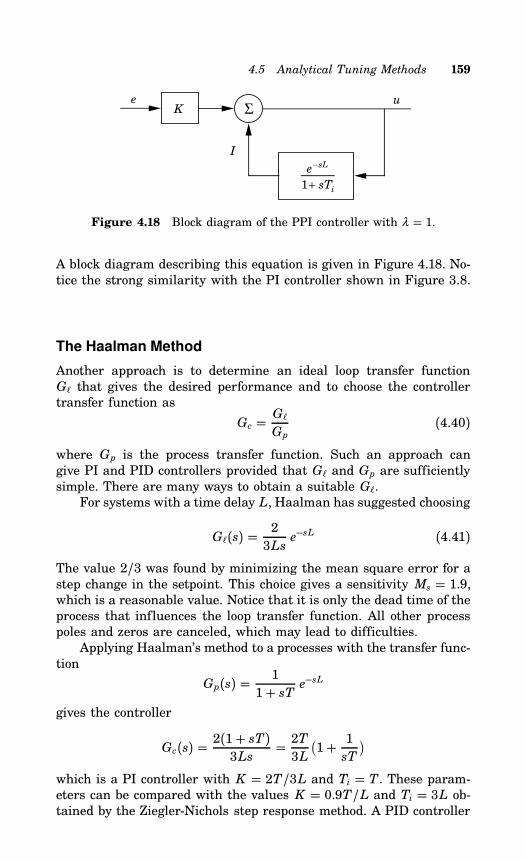
4.5 Analytical Tuning Methods 159
ΣK
e−sL
1+ sTi
e u
I
Figure 4.18 Block diagram of the PPI controller with λ = 1.
A block diagram describing this equation is given in Figure 4.18. No-tice the strong similarity with the PI controller shown in Figure 3.8.
The Haalman Method
Another approach is to determine an ideal loop transfer functionG that gives the desired performance and to choose the controllertransfer function as
Gc = GGp
(4.40)
where Gp is the process transfer function. Such an approach cangive PI and PID controllers provided that G and Gp are sufficientlysimple. There are many ways to obtain a suitable G.For systems with a time delay L, Haalman has suggested choosing
G(s) = 23Ls
e−sL (4.41)
The value 2/3 was found by minimizing the mean square error for astep change in the setpoint. This choice gives a sensitivity Ms = 1.9,which is a reasonable value. Notice that it is only the dead time of theprocess that influences the loop transfer function. All other processpoles and zeros are canceled, which may lead to difficulties.Applying Haalman’s method to a processes with the transfer func-
tion
Gp(s) = 11+ sT e
−sL
gives the controller
Gc(s) = 2(1+ sT)3Ls= 2T3L
(1+ 1sT
)which is a PI controller with K = 2T/3L and Ti = T . These param-eters can be compared with the values K = 0.9T/L and Ti = 3L ob-tained by the Ziegler-Nichols step response method. A PID controller
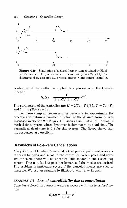
160 Chapter 4 Controller Design
0 10 20 30 40 500
1
0 10 20 30 40 50−1
1
y
ysp
u
Figure 4.19 Simulation of a closed-loop system obtained by Haal-man’s method. The plant transfer function is G(s) = e−s/(s+1). Thediagrams show setpoint ysp, process output y, and control signal u.
is obtained if the method is applied to a process with the transferfunction
Gp(s) = 1(1+ sT1)(1+ sT2) e
−sL
The parameters of the controller are K = 2(T1+T2)/3L, Ti = T1+T2,and Td = T1T2/(T1 + T2).For more complex processes it is necessary to approximate the
processes to obtain a transfer function of the desired form as wasdiscussed in Section 2.9. Figure 4.19 shows a simulation of Haalman’smethod for a system whose dynamics is dominated by dead time. Thenormalized dead time is 0.5 for this system. The figure shows thatthe responses are excellent.
Drawbacks of Pole-Zero Cancellations
A key feature of Haalman’s method is that process poles and zeros arecanceled by poles and zeros in the controller. When poles and zerosare canceled, there will be uncontrollable modes in the closed-loopsystem. This may lead to poor performance if the modes are excited.The problem is particular severe if the canceled modes are slow orunstable. We use an example to illustrate what may happen.
EXAMPLE 4.6 Loss of controllability due to cancellation
Consider a closed-loop system where a process with the transfer func-tion
Gp(s) = 11+ sT e
−sL
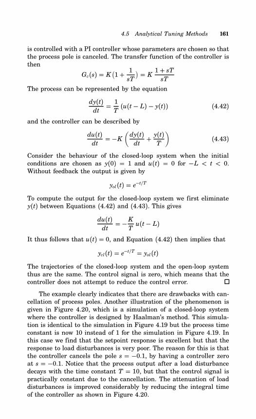
4.5 Analytical Tuning Methods 161
is controlled with a PI controller whose parameters are chosen so thatthe process pole is canceled. The transfer function of the controller isthen
Gc(s) = K(1+ 1sT
) = K 1+ sTsT
The process can be represented by the equation
dy(t)dt= 1T(u(t − L) − y(t)) (4.42)
and the controller can be described by
du(t)dt
= −K(dy(t)dt+ y(t)T
)(4.43)
Consider the behaviour of the closed-loop system when the initialconditions are chosen as y(0) = 1 and u(t) = 0 for −L < t < 0.Without feedback the output is given by
yol(t) = e−t/T
To compute the output for the closed-loop system we first eliminatey(t) between Equations (4.42) and (4.43). This gives
du(t)dt
= −KTu(t− L)
It thus follows that u(t) = 0, and Equation (4.42) then implies that
ycl(t) = e−t/T = yol(t)The trajectories of the closed-loop system and the open-loop systemthus are the same. The control signal is zero, which means that thecontroller does not attempt to reduce the control error.
The example clearly indicates that there are drawbacks with can-cellation of process poles. Another illustration of the phenomenon isgiven in Figure 4.20, which is a simulation of a closed-loop systemwhere the controller is designed by Haalman’s method. This simula-tion is identical to the simulation in Figure 4.19 but the process timeconstant is now 10 instead of 1 for the simulation in Figure 4.19. Inthis case we find that the setpoint response is excellent but that theresponse to load disturbances is very poor. The reason for this is thatthe controller cancels the pole s = −0.1, by having a controller zeroat s = −0.1. Notice that the process output after a load disturbancedecays with the time constant T = 10, but that the control signal ispractically constant due to the cancellation. The attenuation of loaddisturbances is improved considerably by reducing the integral timeof the controller as shown in Figure 4.20.
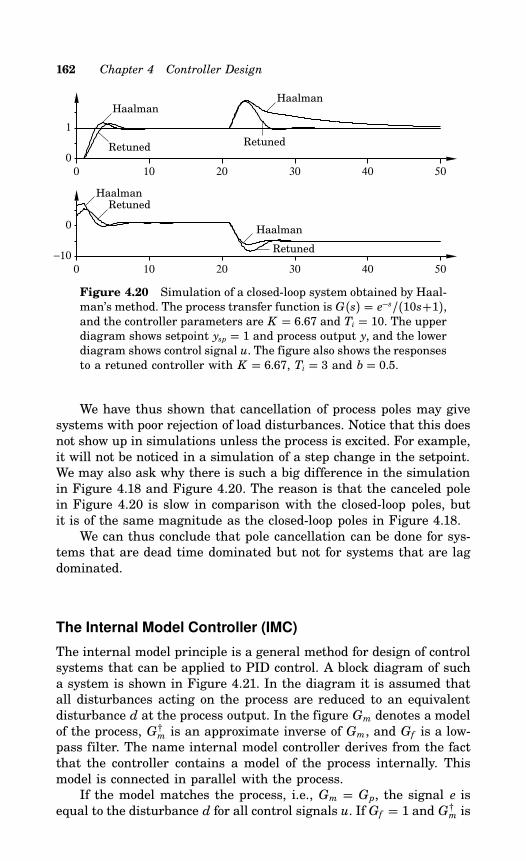
162 Chapter 4 Controller Design
0 10 20 30 40 500
1
0 10 20 30 40 50−10
0
Haalman
Retuned
Haalman
Retuned
HaalmanRetuned
Haalman
Retuned
Figure 4.20 Simulation of a closed-loop system obtained by Haal-man’s method. The process transfer function is G(s) = e−s/(10s+1),and the controller parameters are K = 6.67 and Ti = 10. The upperdiagram shows setpoint ysp = 1 and process output y, and the lowerdiagram shows control signal u. The figure also shows the responsesto a retuned controller with K = 6.67, Ti = 3 and b = 0.5.
We have thus shown that cancellation of process poles may givesystems with poor rejection of load disturbances. Notice that this doesnot show up in simulations unless the process is excited. For example,it will not be noticed in a simulation of a step change in the setpoint.We may also ask why there is such a big difference in the simulationin Figure 4.18 and Figure 4.20. The reason is that the canceled polein Figure 4.20 is slow in comparison with the closed-loop poles, butit is of the same magnitude as the closed-loop poles in Figure 4.18.We can thus conclude that pole cancellation can be done for sys-
tems that are dead time dominated but not for systems that are lagdominated.
The Internal Model Controller (IMC)
The internal model principle is a general method for design of controlsystems that can be applied to PID control. A block diagram of sucha system is shown in Figure 4.21. In the diagram it is assumed thatall disturbances acting on the process are reduced to an equivalentdisturbance d at the process output. In the figure Gm denotes a modelof the process, G†m is an approximate inverse of Gm, and Gf is a low-pass filter. The name internal model controller derives from the factthat the controller contains a model of the process internally. Thismodel is connected in parallel with the process.If the model matches the process, i.e., Gm = Gp, the signal e is
equal to the disturbance d for all control signals u. If Gf = 1 and G†m is
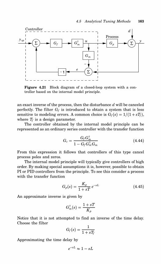
4.5 Analytical Tuning Methods 163
Σ Σ
Σ
u
d
y
Controller
Process
e
−
− 1
y sp
Gf Gm†
Gp
Gm
Figure 4.21 Block diagram of a closed-loop system with a con-troller based on the internal model principle.
an exact inverse of the process, then the disturbance d will be canceledperfectly. The filter Gf is introduced to obtain a system that is lesssensitive to modeling errors. A common choice is Gf (s) = 1/(1+ sTf ),where Tf is a design parameter.The controller obtained by the internal model principle can be
represented as an ordinary series controller with the transfer function
Gc = Gf G†m
1− Gf G†mGm(4.44)
From this expression it follows that controllers of this type cancelprocess poles and zeros.The internal model principle will typically give controllers of high
order. By making special assumptions it is, however, possible to obtainPI or PID controllers from the principle. To see this consider a processwith the transfer function
Gp(s) = Kp
1+ sT e−sL (4.45)
An approximate inverse is given by
G†m(s) =1+ sTKp
Notice that it is not attempted to find an inverse of the time delay.Choose the filter
Gf (s) = 11+ sTf
Approximating the time delay by
e−sL 1− sL
164 Chapter 4 Controller Design
Equation (4.44) now gives
Gc(s) = 1+ sTKps(L+ Tf )
which is a PI controller. If the time delay is approximated instead bya first-order Padé approximation
e−sL 1− sL/21+ sL/2
Equation (4.44) gives instead the PID controller
Gc(s) = (1+ sL/2)(1+ sT)Kps(L + Tf + sTf L/2)
(1+ sL/2)(1+ sT)Kps(L+ Tf )
For processes described by Equation (4.45), we thus find that theinternal model principle will give PI or PID controllers. Approxima-tions like the ones discussed in Section 2.9 can be used in the usualmanner to obtain PI and PID controllers for more complex processes.An interesting feature of the internal model controller is that
robustness is considered explicitly in the design. Robustness can beadjusted by selecting the filter Gf properly. A trade-off between per-formance and robustness can be made by using the filter constant as adesign parameter. The IMC can be designed to give excellent responseto setpoint changes. Since the design method inherently implies thatpoles and zeros of the plant are canceled, the response to load dis-turbances may be poor if the canceled poles are slow in comparisonwith the dominant poles. Compare with the responses in Figure 4.20.The IMC controller can also be viewed as an extension of the Smithpredictor.
4.6 Optimization Methods
Optimization is a powerful tool for design of controllers. The methodis conceptually simple. A controller structure with a few parametersis specified. Specifications are expressed as inequalities of functionsof the parameters. The specification that is most important is cho-sen as the function to optimize. The method is well suited for PIDcontrollers where the controller structure and the parameterizationare given. There are several pitfalls when using optimization. Caremust be exercised when formulating criteria and constraints; other-wise, a criterion will indeed be optimal, but the controller may stillbe unsuitable because of a neglected constraint. Another difficulty isthat the loss function may have many local minima. A third is thatthe computations required may easily be excessive. Numerical prob-lems may also arise. Nevertheless, optimization is a good tool that
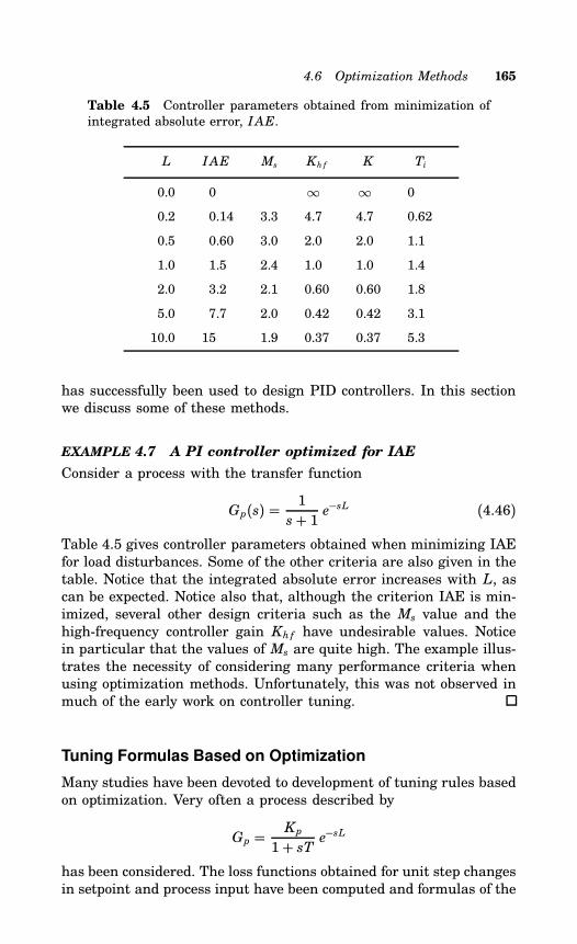
4.6 Optimization Methods 165
Table 4.5 Controller parameters obtained from minimization ofintegrated absolute error, IAE.
L IAE Ms Kh f K Ti
0.0 0 ∞ ∞ 0
0.2 0.14 3.3 4.7 4.7 0.62
0.5 0.60 3.0 2.0 2.0 1.1
1.0 1.5 2.4 1.0 1.0 1.4
2.0 3.2 2.1 0.60 0.60 1.8
5.0 7.7 2.0 0.42 0.42 3.1
10.0 15 1.9 0.37 0.37 5.3
has successfully been used to design PID controllers. In this sectionwe discuss some of these methods.
EXAMPLE 4.7 A PI controller optimized for IAE
Consider a process with the transfer function
Gp(s) = 1s+ 1 e
−sL (4.46)
Table 4.5 gives controller parameters obtained when minimizing IAEfor load disturbances. Some of the other criteria are also given in thetable. Notice that the integrated absolute error increases with L, ascan be expected. Notice also that, although the criterion IAE is min-imized, several other design criteria such as the Ms value and thehigh-frequency controller gain Khf have undesirable values. Noticein particular that the values of Ms are quite high. The example illus-trates the necessity of considering many performance criteria whenusing optimization methods. Unfortunately, this was not observed inmuch of the early work on controller tuning.
Tuning Formulas Based on Optimization
Many studies have been devoted to development of tuning rules basedon optimization. Very often a process described by
Gp = Kp
1+ sT e−sL
has been considered. The loss functions obtained for unit step changesin setpoint and process input have been computed and formulas of the
166 Chapter 4 Controller Design
type
p = a(L
T
)bwhere p is a controller parameter and a and b are constants, havebeen fitted to the numerical values obtained. In many cases thecriterion is IAE for load disturbances, which often gives systems withlow damping and poor sensitivity. The formulas given often only holdfor a small range of normalized dead times, e.g., 0.2 < τ < 0.6. Itshould also be observed that criteria based on setpoint changes canoften be misleading because it is often not observed that the setpointchanges are drastically influenced by different setpoint weightings.
Modulus and Symmetrical Optimum
Modulus Optimum (BO) and Symmetrical Optimum (SO) are twomethods for selecting and tuning controllers that are similar in spiritto Haalman’s method. The acronyms BO and SO are derived from theGerman words Betrags Optimum and Symmetrische Optimum. Thesemethods are based on the idea of finding a controller that makes thefrequency response from setpoint to plant output as close to one aspossible for low frequencies. If G(s) is the transfer function from thesetpoint to the output, the controller is determined in such a waythat G(0) = 1 and that dnG(iω )/dω n = 0 at ω = 0 for as many nas possible. We illustrate the idea with a few examples.
EXAMPLE 4.8 Second-order system
Consider the transfer function
G(s) = a2
s2 + a1s+ a2which has been chosen so that G(0) = 1. Let us first consider howthe parameters should be chosen in order to get a maximally flatfrequency response. We have
G(iω )2 = a22a21ω
2 + (a2 −ω 2)2 =a22
a22 +ω 2(a21 − 2a2) +ω 4
By choosing a1 =√2a2 we find
G(iω )2 = a22a22 +ω 4
The first three derivatives of G(iω ) will vanish at the origin. Thetransfer function then has the form
G(s) = ω 20s2 +√2ω 0s+ω 20
4.6 Optimization Methods 167
The step response of a system with this transfer function has anovershoot o = 4%. The settling time to 2% of the steady state valueis ts = 6/ω 0.If the transfer function G in the example is obtained by error
feedback of a system with the loop transfer function GBO, the looptransfer function is
GBO(s) = G(s)1− G(s) =
ω 20s(s+
√2ω 0)
(4.47)
which is the desired loop transfer function for the method calledmodulus optimum.The calculation in Example 4.8 can be performed for higher-order
systems with more effort. We illustrate by another example.
EXAMPLE 4.9 Third-order system
Consider the transfer function
G(s) = a3
s3 + a1s2 + a2s+ a3After some calculations we get
G(iω ) = a3√a23 + (a22 − 2a1a3)ω 2 + (a21 − 2a2)ω 4 +ω 6
Five derivatives of G(iω ) will vanish at ω = 0, if the parametersare such that a21 = 2a2 and a22 = 2a1a3. The transfer function thenbecomes
G(s) = ω 30s3 + 2ω 0s2 + 2ω 20s+ω 30
= ω 30(s+ω 0)(s2 +ω 0s+ω 20)
(4.48)
The step response of a system with this transfer function has anovershoot o = 8.1%. The settling time to 2% of the steady state valueis 9.4/ω 0. A system with this closed-loop transfer function can beobtained with a system having error feedback and the loop transferfunction
G(s) = ω 30s(s2 + 2ω 0s+ 2ω 20)
The closed-loop transfer function (4.48) can also be obtained fromother loop transfer functions if a two-degree of freedom controller isused. For example, if a process with the transfer function
Gp(s) = ω 20s(s+ 2ω 0)
168 Chapter 4 Controller Design
is controlled by a PI controller having parameters K = 2, Ti = 2/ω 0and b = 0, the loop transfer function becomes
GSO = ω 20(2s+ω 0)s2(s+ 2ω 0) (4.49)
The symmetric optimum aims at obtaining the loop transfer functiongiven by Equation (4.49). Notice that the Bode diagram of this trans-fer function is symmetrical around the frequency ω = ω 0. This is themotivation for the name symmetrical optimum.If a PI controller with b = 1 is used, the transfer function from
setpoint to process output becomes
G(s) = GSO(s)1+ GSO(s) =
(2s+ω 0)ω 20(s+ω 0)(s2 +ω 0s+ω 20)
This transfer function is not maximally flat because of the zero in thenumerator. This zero will also give a setpoint response with a largeovershoot, about 43%.
The methods BO and SO can be called loop-shaping methodssince both methods try to obtain a specific loop transfer function.The design methods can be described as follows. It is first establishedwhich of the transfer functions, GBO or GSO, is most appropriate.The transfer function of the controller Gc(s) is then chosen so thatG(s) = Gc(s)Gp(s), where G is the chosen loop transfer function.We illustrate the methods with the following examples.
EXAMPLE 4.10 BO control
Consider a process with the transfer function
Gp(s) = Kp
s(1+ sT) (4.50)
With a proportional controller the loop transfer function becomes
G(s) = K Kp
s(1+ sT)To make this transfer function equal to GBO given by Equation (4.47)it must be required that
ω 0 =√22T
The controller gain should be chosen as
K = ω 0√2
2Kp= 12KpT
4.6 Optimization Methods 169
EXAMPLE 4.11 SO control
Consider a process with the same transfer function as in the previousexample (Equation (4.50)). With a PI controller having the transferfunction
Gc(s) = K (1+ sTi)sTi
we obtain the loop transfer function
G(s) = KpK (1+ sTi)s2Ti(1+ sT)
This is identical to GSO if we choose
K = 12KpT
Ti = 4TTo obtain the transfer function given by Equation (4.48) betweensetpoint and process output, the controller should have the input-output relation
u(t) = K(−y(t) + 1
Ti
∫ t
(ysp(s) − y(s)) ds)
The coefficient b in the standard controller thus should be set to zero.
A Design Procedure
A systematic design procedure can be based on the methods BO andSO. The design method consists of two steps. In the first step theprocess transfer function is simplified to one of the following forms
G1(s) = Kp
1+ sT (4.51)
G2(s) = Kp
(1+ sT1)(1+ sT2) , T1 > T2 (4.52)
G3(s) = Kp
(1+ sT1)(1+ sT2)(1+ sT3) , T1 > T2 > T3 (4.53)
G4(s) = Kp
s(1+ sT) (4.54)
G5(s) = Kp
s(1+ sT1)(1+ sT2) , T1 > T2 (4.55)
Process poles may be canceled by controller zeros to obtain the desiredloop transfer function. A slow pole may be approximated by an inte-grator; fast poles may be lumped together as discussed in Section 2.9.
170 Chapter 4 Controller Design
The rule of thumb given in the original papers on the method is thattime constants such that ω 0T < 0.25 can be regarded as integrators.The controller is derived in the same way as in Examples 4.10
and 4.11 by choosing parameters so that the loop transfer functionmatches either GBO or GSO. By doing this we obtain the resultssummarized in Table 4.6. Notice, for example, that Example 4.10 and4.11 correspond to the entries Process G4 in the table. It is naturalto view the smallest time constant as an approximation of neglecteddynamics in the process. It is interesting to observe that it is this timeconstant that determines the bandwidth of the closed-loop system.The setpoint response for the BO method is excellent. Notice
that it is necessary to use a controller with a two-degree-of-freedomstructure or a prefilter to avoid a high overshoot for the SO method.Notice that process poles are canceled in the cases marked C1 or C2in Table 4.6. The response to load disturbances will be poor if thecanceled pole is slow compared to the closed-loop dynamics, which ischaracterized by ω 0 in Table 4.6.These design principles can be extended to processes other than
those listed in the table.
EXAMPLE 4.12 Application of BO and SO
Consider a process with the transfer function
G(s) = 1(1+ s)(1+ 0.2s)(1+ 0.05s)(1+ 0.01s) (4.56)
Since this transfer function is of fourth order, the design procedurecannot be applied directly. We show how different controllers are ob-tained depending on the approximations made. The performance ofthe closed-loop system depends on the approximation. We use param-eter ω 0 as a crude measure of performance.If a controller with low performance is acceptable, the process
(4.56) can be approximated with
G(s) = 11+ 1.26s (4.57)
The approximation has a phase error less than 10 for ω ≤ 1.12. Itfollows from Table 4.6 that the system (4.57) can be controlled withan integrating controller with
ki = KTi= 0.51.26
= 0.4This gives a closed-loop system with ω 0 = 0.55.A closed-loop system with better performance is obtained if the
transfer function (4.56) is approximated with
G(s) = 1(1+ s)(1+ 0.26s) (4.58)
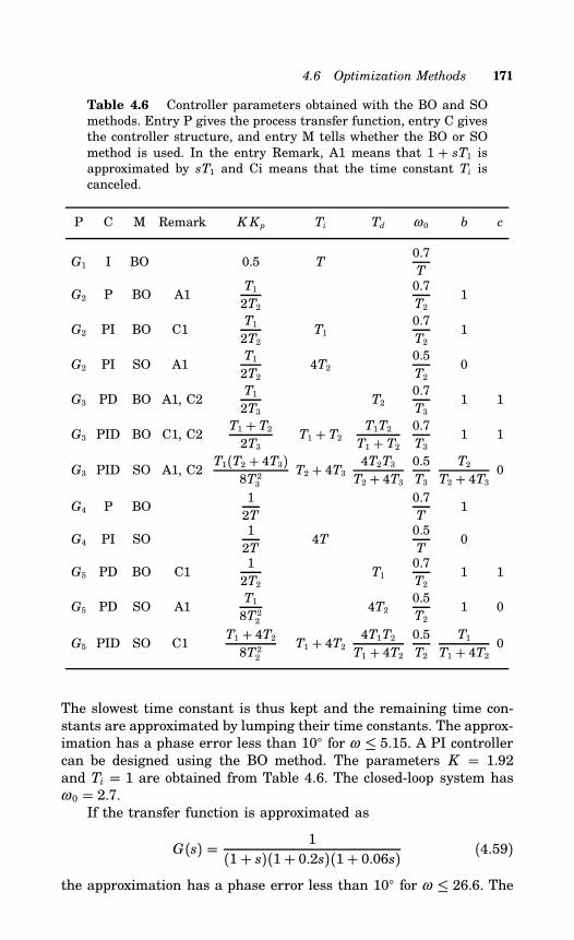
4.6 Optimization Methods 171
Table 4.6 Controller parameters obtained with the BO and SOmethods. Entry P gives the process transfer function, entry C givesthe controller structure, and entry M tells whether the BO or SOmethod is used. In the entry Remark, A1 means that 1 + sT1 isapproximated by sT1 and Ci means that the time constant Ti iscanceled.
P C M Remark KKp Ti Td ω 0 b c
G1 I BO 0.5 T0.7T
G2 P BO A1T1
2T2
0.7T2
1
G2 PI BO C1T1
2T2T1
0.7T2
1
G2 PI SO A1T1
2T24T2
0.5T2
0
G3 PD BO A1, C2T1
2T3T2
0.7T3
1 1
G3 PID BO C1, C2T1 + T22T3
T1 + T2 T1T2
T1 + T20.7T3
1 1
G3 PID SO A1, C2T1(T2 + 4T3)
8T23T2 + 4T3 4T2T3
T2 + 4T30.5T3
T2
T2 + 4T3 0
G4 P BO12T
0.7T
1
G4 PI SO12T
4T0.5T
0
G5 PD BO C112T2
T10.7T2
1 1
G5 PD SO A1T1
8T224T2
0.5T2
1 0
G5 PID SO C1T1 + 4T28T22
T1 + 4T2 4T1T2T1 + 4T2
0.5T2
T1
T1 + 4T2 0
The slowest time constant is thus kept and the remaining time con-stants are approximated by lumping their time constants. The approx-imation has a phase error less than 10 for ω ≤ 5.15. A PI controllercan be designed using the BO method. The parameters K = 1.92and Ti = 1 are obtained from Table 4.6. The closed-loop system hasω 0 = 2.7.If the transfer function is approximated as
G(s) = 1(1+ s)(1+ 0.2s)(1+ 0.06s) (4.59)
the approximation has a phase error less than 10 for ω ≤ 26.6. The
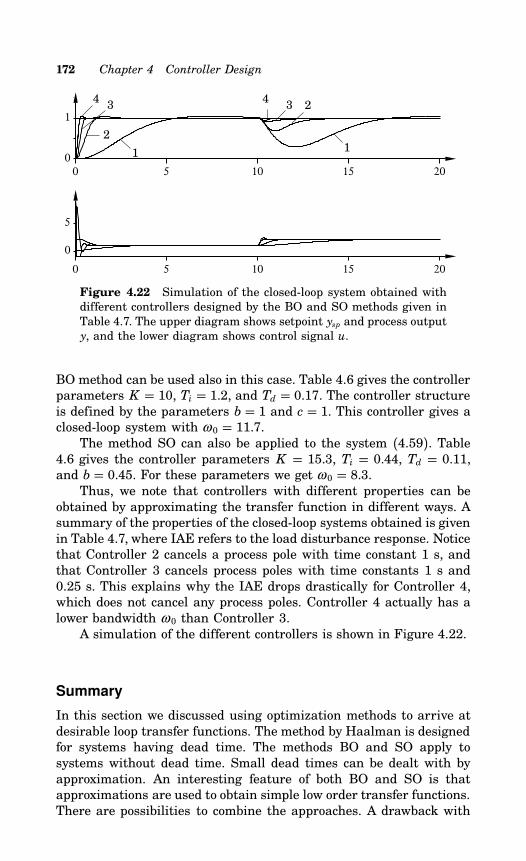
172 Chapter 4 Controller Design
0 5 10 15 200
1
0 5 10 15 20
0
5
4 3
2
1
4 3 2
1
Figure 4.22 Simulation of the closed-loop system obtained withdifferent controllers designed by the BO and SO methods given inTable 4.7. The upper diagram shows setpoint ysp and process outputy, and the lower diagram shows control signal u.
BO method can be used also in this case. Table 4.6 gives the controllerparameters K = 10, Ti = 1.2, and Td = 0.17. The controller structureis defined by the parameters b = 1 and c = 1. This controller gives aclosed-loop system with ω 0 = 11.7.The method SO can also be applied to the system (4.59). Table
4.6 gives the controller parameters K = 15.3, Ti = 0.44, Td = 0.11,and b = 0.45. For these parameters we get ω 0 = 8.3.Thus, we note that controllers with different properties can be
obtained by approximating the transfer function in different ways. Asummary of the properties of the closed-loop systems obtained is givenin Table 4.7, where IAE refers to the load disturbance response. Noticethat Controller 2 cancels a process pole with time constant 1 s, andthat Controller 3 cancels process poles with time constants 1 s and0.25 s. This explains why the IAE drops drastically for Controller 4,which does not cancel any process poles. Controller 4 actually has alower bandwidth ω 0 than Controller 3.A simulation of the different controllers is shown in Figure 4.22.
Summary
In this section we discussed using optimization methods to arrive atdesirable loop transfer functions. The method by Haalman is designedfor systems having dead time. The methods BO and SO apply tosystems without dead time. Small dead times can be dealt with byapproximation. An interesting feature of both BO and SO is thatapproximations are used to obtain simple low order transfer functions.There are possibilities to combine the approaches. A drawback with
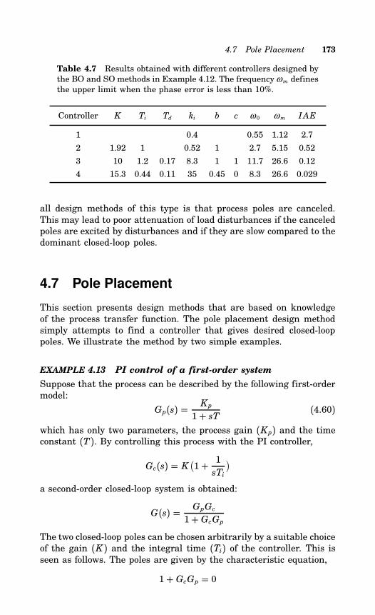
4.7 Pole Placement 173
Table 4.7 Results obtained with different controllers designed bythe BO and SO methods in Example 4.12. The frequencyωm definesthe upper limit when the phase error is less than 10%.
Controller K Ti Td ki b c ω 0 ωm IAE
1 0.4 0.55 1.12 2.7
2 1.92 1 0.52 1 2.7 5.15 0.52
3 10 1.2 0.17 8.3 1 1 11.7 26.6 0.12
4 15.3 0.44 0.11 35 0.45 0 8.3 26.6 0.029
all design methods of this type is that process poles are canceled.This may lead to poor attenuation of load disturbances if the canceledpoles are excited by disturbances and if they are slow compared to thedominant closed-loop poles.
4.7 Pole Placement
This section presents design methods that are based on knowledgeof the process transfer function. The pole placement design methodsimply attempts to find a controller that gives desired closed-looppoles. We illustrate the method by two simple examples.
EXAMPLE 4.13 PI control of a first-order system
Suppose that the process can be described by the following first-ordermodel:
Gp(s) = Kp
1+ sT (4.60)
which has only two parameters, the process gain (Kp) and the timeconstant (T). By controlling this process with the PI controller,
Gc(s) = K(1+ 1sTi
)a second-order closed-loop system is obtained:
G(s) = GpGc
1+ GcGpThe two closed-loop poles can be chosen arbitrarily by a suitable choiceof the gain (K ) and the integral time (Ti) of the controller. This isseen as follows. The poles are given by the characteristic equation,
1+ GcGp = 0
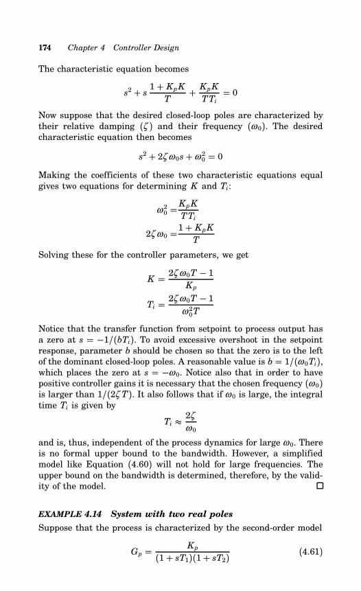
174 Chapter 4 Controller Design
The characteristic equation becomes
s2 + s 1+ KpKT
+ KpKTTi
= 0
Now suppose that the desired closed-loop poles are characterized bytheir relative damping (ζ ) and their frequency (ω 0). The desiredcharacteristic equation then becomes
s2 + 2ζ ω 0s+ω 20 = 0Making the coefficients of these two characteristic equations equalgives two equations for determining K and Ti:
ω 20 =KpK
TTi
2ζ ω 0 =1+ KpKT
Solving these for the controller parameters, we get
K = 2ζ ω 0T − 1Kp
Ti = 2ζ ω 0T − 1ω 20T
Notice that the transfer function from setpoint to process output hasa zero at s = −1/(bTi). To avoid excessive overshoot in the setpointresponse, parameter b should be chosen so that the zero is to the leftof the dominant closed-loop poles. A reasonable value is b = 1/(ω 0Ti),which places the zero at s = −ω 0. Notice also that in order to havepositive controller gains it is necessary that the chosen frequency (ω 0)is larger than 1/(2ζ T). It also follows that if ω 0 is large, the integraltime Ti is given by
Ti 2ζω 0
and is, thus, independent of the process dynamics for large ω 0. Thereis no formal upper bound to the bandwidth. However, a simplifiedmodel like Equation (4.60) will not hold for large frequencies. Theupper bound on the bandwidth is determined, therefore, by the valid-ity of the model.
EXAMPLE 4.14 System with two real poles
Suppose that the process is characterized by the second-order model
Gp = Kp
(1+ sT1)(1+ sT2) (4.61)
4.7 Pole Placement 175
This model has three parameters. By using a PID controller, whichalso has three parameters, it is possible to arbitrarily place the threepoles of the closed-loop system. The transfer function of the PIDcontroller can be written as
Gc(s) = K (1+ sTi + s2TiTd)
sTi
The characteristic equation of the closed-loop system becomes
s3 + s2( 1Ti+ 1T2+ KpKTdT1T2
)+ s( 1T1T2
+ KpKT1T2
)+ KpK
T1T2Ti= 0 (4.62)
A suitable closed-loop characteristic equation of a third-order systemis
(s+αω 0)(s2 + 2ζ ω 0s+ω 20) = 0 (4.63)which contains two dominant poles with relative damping (ζ ) andfrequency (ω 0), and a real pole located in −αω 0. Identifying thecoefficients of equal powers of s in the Equations (4.62) and (4.63)gives
1Ti+ 1T2+ KpKTdT1T2
= ω 0(α + 2ζ )1T1T2
+ KpKT1T2
= ω 20(1+ 2ζ ω 0)KpK
T1T2Ti= αω 30
Solving these equations gives the following controller parameters
K = T1T2ω20(1+ 2αζ ) − 1Kp
Ti = T1T2ω20(1+ 2αζ ) − 1T1T2αω 30
Td = T1T2ω 0(α + 2ζ ) − T1 − T2T1T2ω 20(1+ 2αζ ) − 1
Provided that c = 0, the transfer function from setpoint to processoutput has one zero at s = −1/(bTi). To avoid excessive overshoot inthe setpoint response, parameter b can be chosen so that this zerocancels the pole at s = −αω 0. This gives
b = 1αω 0Ti
= ω 20T1T2ω 20T1T2(1+ 2αζ ) − 1
Also, notice that pure PI control is obtained for
ω 0 = ω c = T1 + T2(α + 2ζ )T1T2
176 Chapter 4 Controller Design
The choice of ω 0 may be critical. The derivative time is negativefor ω 0 < ω c. Thus, the frequency (ω c) gives a lower bound to thebandwidth. The gain increases rapidly with ω 0. The upper boundto the bandwidth is given by the validity of the simplified model(Equation 4.61).The methods BO and SO, discussed in the previous section, can
clearly be interpreted as pole placement methods. The desired closed-loop characteristic polynomial is
ABO(s) = s2 +√2ω 0s+ω 20
for the modulus optimum and
ASO(s) = (s+ω 0)(s2 +ω 0s+ω 20)for the symmetrical optimum.The calculations in Example 4.14 can be done for any linear sys-
tem. The algebraic formulas obtained, however, may be quite compli-cated. Another useful example follows.
EXAMPLE 4.15 Second-order systems with a zero
Suppose that the process is characterized by the second-order model
Gp = b1s+ b2s2 + a1s+ a2 (4.64)
This model has four parameters. It has two poles that may be realor complex, and it has one zero. The model given by Equation (4.64)captures many processes, oscillatory systems, and systems with righthalf-plane zeros. The right half-plane zero can also be used as an ap-proximation of a time delay. We assume that the process is controlledby a PID controller parameterized as
Gc(s) = k+ kis+ kds (4.65)
The closed-loop system is of third order and has the characteristicequation
s(s2 + a1s+ a2) + (b1s+ b2)(kds2 + ks+ ki) = 0 (4.66)A suitable closed-loop characteristic equation of a third-order systemis
(s+αω 0)(s2 + 2ζ ω 0s+ω 20) = 0 (4.67)Equating coefficients of equal power in s in Equations (4.66) and(4.67) gives the following equations:
a1 + b2kd + b1k = (αω 0 + 2ζ ω 0)(1+ b1kd)a2 + b2k+ b1ki = (1+ 2αζ )ω 20(1+ b1kd)
b2ki = αω 30(1+ b1kd)
4.7 Pole Placement 177
This is a set of linear equations in the controller parameters. Thesolution is straightforward but tedious and is given by
k = a2b22− a2b1b2(α + 2ζ )ω 0−(b2− a1b1)(b2(1+ 2αζ )ω 20 +α b1ω
30)
b32− b1b22(α + 2ζ )ω 0+ b21b2(1+ 2αζ )ω 20−α b31ω30
ki = (−a1b1b2+ a2b21+ b22)αω 30b32− b1b22(α + 2ζ )ω 0+ b21b2(1+ 2αζ )ω 20−α b31ω
30
kd = −a1b22+ a2b1b2+ b22(α + 2ζ )ω 0− b1b2ω 20(1+ 2αζ )+ b21αω 30b32− b1b22(α + 2ζ )ω 0+ b21b2(1+ 2αζ )ω 20−α b31ω
30
These formulas are quite useful because many processes can be ap-proximately described by the transfer function given by Equation(4.64).The formulas given in Example 4.15 are particularly useful in
cases when we are “stretching” the PID controller to extreme situa-tions. The standard tuning rules will typically not work in these cases.Typical examples are systems with zeros in the right half-plane andsystems with poorly damped oscillatory modes. To illustrate this wewill consider an example.
EXAMPLE 4.16 A difficult process
Consider a system with the transfer function
G(s) = 1− ss2 + 1
This system has one right half-plane zero and two undamped complexpoles. None of the standard methods for tuning PID controllers workwell for this system. To apply the pole-placement method we requirethat the closed-loop system has the characteristic equation
s3 + 2s2 + 2s+ 1 = 0The formulas in Example 4.15 give a controller with the parametersk = 0, ki = 1/3, and kd = 2/3. This can also be verified with asimple calculation. Notice that the proportional gain is zero and thatthe controller has two complex zeros at ±i
√2. Such a controller can
only be implemented with a PID controller having the parallel form.Compare with section 3.4.
The General Case
The calculations in the examples can be extended to general linearsystems. They are, however, more complicated. It is necessary to spec-
178 Chapter 4 Controller Design
ify more closed-loop poles. Some pole patterns that are used are But-terworth configurations, where the roots of the characteristic polyno-mials are placed symmetrically in a circle, and the Bessel configura-tions, which correspond to filters that attempt to preserve the shapeof the wave form. The order of the controllers also increases with thecomplexity of the model. To obtain PID controllers it is necessary torestrict the models to first- or second-order systems. For more complexprocesses, it is, therefore, necessary to make approximations so thata process model in the form of a rational function of first or secondorder is obtained. Several ways to perform these approximations areegiven in Chapter 2. We illustrate the procedure with an example.
EXAMPLE 4.17 Pole placement with an approximate model
Consider a process described by the transfer function
Gp(s) = 1(1+ s)(1+ 0.2s)(1+ 0.05s)(1+ 0.01s) (4.68)
This process has four lags with time constants 1, 0.2, 0.05, and 0.01.The approximations can be done in several different ways. If the con-trol requirements are not too severe, we can attempt to approximatethe transfer function by
Gp(s) = 11+ 1.26s
where the time constant is the average residence time of the system.As discussed in Section 2.9, this approximation is good at low fre-quencies. The phase error is less than 10 for frequencies below 1.1rad/s. Designing a PI controller with the pole placement method withζ = 0.5, the following controller parameters are obtained
K = 1.26ω 0 − 1
Ti = 1.26ω 0 − 11.26ω 20
b = 1.26ω 01.26ω 0 − 1
where b is chosen so that the zero becomes s = −ω 0. If the processmodel would be correct, the phase margin with ζ = 0.5 would be 50.Because of the approximations made, the phase margin will be less. Itwill decrease with ω 0. For ω 0 = 1 the phase margin is ϕm = 42.Another way of applying pole placement design is given in the
next example.
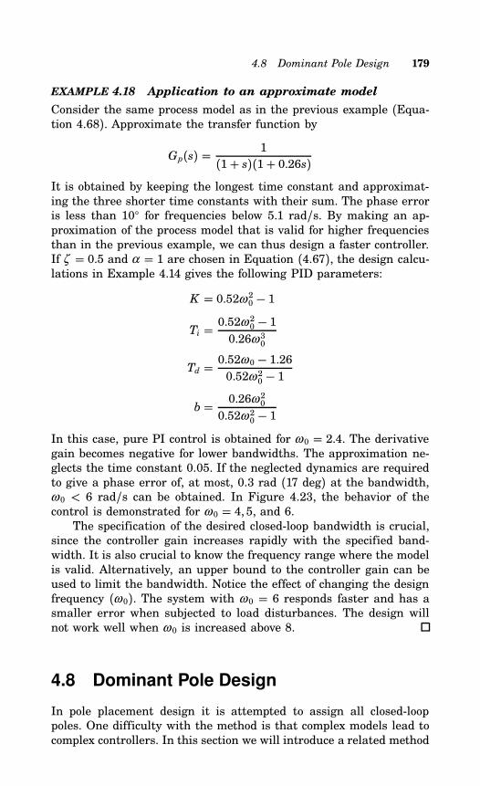
4.8 Dominant Pole Design 179
EXAMPLE 4.18 Application to an approximate model
Consider the same process model as in the previous example (Equa-tion 4.68). Approximate the transfer function by
Gp(s) = 1(1+ s)(1+ 0.26s)
It is obtained by keeping the longest time constant and approximat-ing the three shorter time constants with their sum. The phase erroris less than 10 for frequencies below 5.1 rad/s. By making an ap-proximation of the process model that is valid for higher frequenciesthan in the previous example, we can thus design a faster controller.If ζ = 0.5 and α = 1 are chosen in Equation (4.67), the design calcu-lations in Example 4.14 gives the following PID parameters:
K = 0.52ω 20 − 1
Ti = 0.52ω20 − 1
0.26ω 30
Td = 0.52ω 0 − 1.260.52ω 20 − 1
b = 0.26ω 200.52ω 20 − 1
In this case, pure PI control is obtained for ω 0 = 2.4. The derivativegain becomes negative for lower bandwidths. The approximation ne-glects the time constant 0.05. If the neglected dynamics are requiredto give a phase error of, at most, 0.3 rad (17 deg) at the bandwidth,ω 0 < 6 rad/s can be obtained. In Figure 4.23, the behavior of thecontrol is demonstrated for ω 0 = 4, 5, and 6.The specification of the desired closed-loop bandwidth is crucial,
since the controller gain increases rapidly with the specified band-width. It is also crucial to know the frequency range where the modelis valid. Alternatively, an upper bound to the controller gain can beused to limit the bandwidth. Notice the effect of changing the designfrequency (ω 0). The system with ω 0 = 6 responds faster and has asmaller error when subjected to load disturbances. The design willnot work well when ω 0 is increased above 8.
4.8 Dominant Pole Design
In pole placement design it is attempted to assign all closed-looppoles. One difficulty with the method is that complex models lead tocomplex controllers. In this section we will introduce a related method
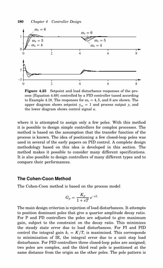
180 Chapter 4 Controller Design
0 2 4 6 80
1
0 2 4 6 8−5
5
ω 0 = 6
ω 0 = 5ω 0 = 4
ω 0 = 6ω 0 = 5
ω 0 = 4
Figure 4.23 Setpoint and load disturbance responses of the pro-cess (Equation 4.68) controlled by a PID controller tuned accordingto Example 4.18. The responses for ω 0 = 4, 5, and 6 are shown. Theupper diagram shows setpoint ysp = 1 and process output y, andthe lower diagram shows control signal u.
where it is attempted to assign only a few poles. With this methodit is possible to design simple controllers for complex processes. Themethod is based on the assumption that the transfer function of theprocess is known. The idea of positioning a few closed-loop poles wasused in several of the early papers on PID control. A complete designmethodology based on this idea is developed in this section. Themethod makes it possible to consider many different specifications.It is also possible to design controllers of many different types and tocompare their performances.
The Cohen-Coon Method
The Cohen-Coon method is based on the process model
Gp = Kp
1+ sT e−sL
The main design criterion is rejection of load disturbances. It attemptsto position dominant poles that give a quarter amplitude decay ratio.For P and PD controllers the poles are adjusted to give maximumgain, subject to the constraint on the decay ratio. This minimizesthe steady state error due to load disturbances. For PI and PIDcontrol the integral gain ki = K/Ti is maximized. This correspondsto minimization of IE, the integral error due to a unit step loaddisturbance. For PID controllers three closed-loop poles are assigned;two poles are complex, and the third real pole is positioned at thesame distance from the origin as the other poles. The pole pattern is
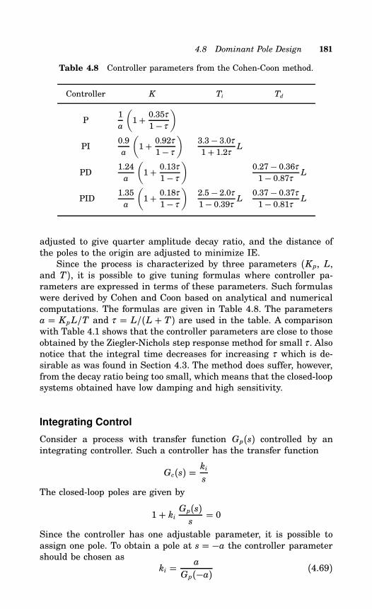
4.8 Dominant Pole Design 181
Table 4.8 Controller parameters from the Cohen-Coon method.
Controller K Ti Td
P1a
(1+ 0.35τ
1− τ
)
PI0.9a
(1+ 0.92τ
1− τ
)3.3− 3.0τ1+ 1.2τ L
PD1.24a
(1+ 0.13τ
1− τ
)0.27− 0.36τ1− 0.87τ L
PID1.35a
(1+ 0.18τ
1− τ
)2.5− 2.0τ1− 0.39τ L
0.37− 0.37τ1− 0.81τ L
adjusted to give quarter amplitude decay ratio, and the distance ofthe poles to the origin are adjusted to minimize IE.Since the process is characterized by three parameters (Kp, L,
and T), it is possible to give tuning formulas where controller pa-rameters are expressed in terms of these parameters. Such formulaswere derived by Cohen and Coon based on analytical and numericalcomputations. The formulas are given in Table 4.8. The parametersa = KpL/T and τ = L/(L + T) are used in the table. A comparisonwith Table 4.1 shows that the controller parameters are close to thoseobtained by the Ziegler-Nichols step response method for small τ . Alsonotice that the integral time decreases for increasing τ which is de-sirable as was found in Section 4.3. The method does suffer, however,from the decay ratio being too small, which means that the closed-loopsystems obtained have low damping and high sensitivity.
Integrating Control
Consider a process with transfer function Gp(s) controlled by anintegrating controller. Such a controller has the transfer function
Gc(s) = kis
The closed-loop poles are given by
1+ ki Gp(s)s= 0
Since the controller has one adjustable parameter, it is possible toassign one pole. To obtain a pole at s = −a the controller parametershould be chosen as
ki = a
Gp(−a) (4.69)
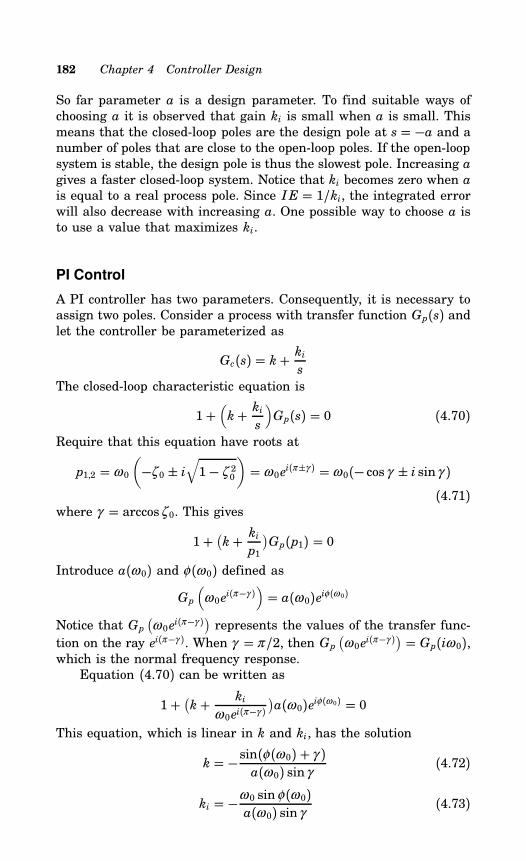
182 Chapter 4 Controller Design
So far parameter a is a design parameter. To find suitable ways ofchoosing a it is observed that gain ki is small when a is small. Thismeans that the closed-loop poles are the design pole at s = −a and anumber of poles that are close to the open-loop poles. If the open-loopsystem is stable, the design pole is thus the slowest pole. Increasing agives a faster closed-loop system. Notice that ki becomes zero when ais equal to a real process pole. Since IE = 1/ki, the integrated errorwill also decrease with increasing a. One possible way to choose a isto use a value that maximizes ki.
PI Control
A PI controller has two parameters. Consequently, it is necessary toassign two poles. Consider a process with transfer function Gp(s) andlet the controller be parameterized as
Gc(s) = k+ kis
The closed-loop characteristic equation is
1+(k+ ki
s
)Gp(s) = 0 (4.70)
Require that this equation have roots at
p1,2 = ω 0
(−ζ 0 ± i
√1− ζ 20
)= ω 0e
i(π±γ ) = ω 0(− cos γ ± i sinγ )(4.71)
where γ = arccosζ 0. This gives
1+ (k+ kip1
)Gp(p1) = 0
Introduce a(ω 0) and φ(ω 0) defined asGp
(ω 0e
i(π−γ ))= a(ω 0)eiφ(ω 0)
Notice that Gp(ω 0e
i(π−γ )) represents the values of the transfer func-tion on the ray ei(π−γ ). When γ = π/2, then Gp
(ω 0e
i(π−γ )) = Gp(iω 0),which is the normal frequency response.Equation (4.70) can be written as
1+ (k+ ki
ω 0ei(π−γ ))a(ω 0)eiφ(ω 0) = 0
This equation, which is linear in k and ki, has the solution
k = −sin(φ(ω 0) + γ )a(ω 0) sinγ
(4.72)
ki = −ω 0 sinφ(ω 0)a(ω 0) sin γ
(4.73)
4.8 Dominant Pole Design 183
Notice that φ(ω 0) is zero for ω 0 = 0 and typically negative as ω 0increases. This implies that the proportional gain is negative and theintegral gain positive but small for small ω 0. When ω 0 increases bothk and ki will increase initially. For larger values ofω 0 both parameterswill decrease. Requiring that both parameters are positive, we findthat ω 0 must be selected so that
γ < −φ(ω 0) < π
The integral time of the controller is
Ti = kki= sin(φ(ω 0) + γ )
ω 0 sinφ(ω 0) (4.74)
Notice that Ti is independent of a(ω 0).
PD Control
A PD controller has two parameters. To obtain these it is necessaryto specify two closed-loop poles. The controller is assumed to be pa-rameterized as
Gc(s) = k+ kdsSpecifying the desired poles as
p1,2 = ω 0(−ζ 0 ± i
√1− ζ 20
)and proceeding as in the derivation of the PI controller we find
k = sin(φ(ω 0) − γ )a(ω 0) sinγ
(4.75)
kd = sinφ(ω 0)ω 0a(ω 0) sinγ
(4.76)
Note that the expressions of k and kd for PD controllers are similarto those of PI controllers.
PID Control
Now we consider PID control. For simplicity, it is assumed that thecontroller is parameterized as
Gc(s) = k+ kis+ kds (4.77)
Modifications in the setpoint weighting and limitation of the deriva-tive gain are taken care of later. Since the controller has three param-eters, it is necessary to specify three poles of the closed-loop system.
184 Chapter 4 Controller Design
We choose them as
p1,2 = ω 0
(−ζ 0 ± i
√1− ζ 20
)(4.78)
p3 = −α 0ω 0. (4.79)Introduce the quantities a(ω 0), b(ω 0), and φ(ω 0) defined by
Gp
(ω 0e
i(π−γ ))= a(ω 0)eiφ(ω 0)
Gp(−αω 0) = −b(ω 0)The condition that p1, p2, and p3 are roots of
1+ Gp(s)Gc(s) = 0 (4.80)gives the conditions
k = −α 20b(ω 0) sin (γ + φ) + b(ω 0) sin (γ − φ) +α 0a(ω 0) sin 2γa(ω 0)b(ω 0)(α 20 − 2α 0 cosγ + 1) sin γ
ki = −α 0ω 0a(ω 0) sinγ + b(ω 0)(sin (γ − φ) +α 0 sinφ)a(ω 0)b(ω 0)(α 20 − 2α 0 cosγ + 1) sinγ
kd = −α 0a(ω 0) sinγ + b(ω 0)(α 0 sin (γ + φ) − sinφ)ω 0a(ω 0)b(ω 0)(α 20 − 2α 0 cosγ + 1) sin γ
PID Controller Based on PI Controller
Another way to obtain a PID controller is to start with a PI controllerand to add derivative action. This can be done as follows. Assumethat the controller
Gc(s) = k+ kis+ kds (4.81)
is used and that it is desired to have two closed-loop poles in
p1,2 = ω 0
(−ζ 0 ± i
√1− ζ 20
)
The value of the controller transfer function at these poles can bewritten as
Gc(p1) = k+ kiω 0e−i(π−γ ) + kdω 0ei(π−γ )
= k−(kdω 0 + ki
ω 0
)cosγ + i
(kdω 0 − ki
ω 0
)sin γ
This implies that
k = k′ + 2kdζ 0ω 0ki = k′i + kdω 20
4.8 Dominant Pole Design 185
where k′ and k′i are the controller parameters for a pure PI controllergiven by Equations (4.72) and (4.73). Using this parameterization thePID controller can be written
Gc(s) = G ′c(s) +kd
s
(s2 + 2ζ 0ω 0s+ω 20
) (4.82)
where G ′c(s) is a pure PI controller, i.e., Gc(s) with kd = 0. The taskis now to choose ζ 0, ω 0, and kd such that the system behaves well.The characteristic equation of the closed-loop system becomes
1+Gp(s)Gc(s) = 1+Gp(s)(G ′c(s) +
kd
s
(s2 + 2ζ 0ω 0s+ω 20
))(4.83)
For a system controlled by a PI controller we have
1+ Gp(s)G ′c(s) =(s2 + 2ζ 0ω 0s+ω 20
)R(s)
The zeros of R(s) are the free poles of the system controlled by thePI controller G ′c(s). Thus,
1+ Gp(s)Gc(s) =(s2 + 2ζ 0ω 0s+ω 20
)(R(s) + Gp(s) kd
s
)(4.84)
The root locus of 1 + Gp(s)Gc(s) with respect to kd will start in thezeros of R(s) and end in the zeros of Gp(s) or in infinity.This parameterization offers a natural way to tune a PID con-
troller: start with a well tuned PI controller and add derivative ac-tion. As kd is increased the parameter ω 0 may have to be modified,e.g., in such a way that IE is maximized.
PID Controller Based on PD controller
Another way to obtain a PID controller is to start with a PD controllerand to add integral action. Proceeding in the same way as previouslybut starting with a PD controller we get
k = k′′ + 2kiζ 0ω 0
kd = k′′d +ki
ω 20
where k′′ and k′′d are the controller parameters for a pure PD controllergiven by Equations (4.75) and (4.76).
A Design Procedure
We have shown that it is possible to find controllers that assign asmany closed-loop poles as there are free parameters in the controller.
186 Chapter 4 Controller Design
The calculations required are simply a solution of a set of linearequations. For a PI controller it is possible to assign a pair of complexpoles with given frequency ω 0 and relative damping ζ 0. The assignedpoles will be dominating if the frequency is sufficiently small. Wecan use this idea to develop systematic design procedures. To doso we start with a set of specifications and design parameters. Thespecifications considered are to express load disturbance rejection,sensitivity to measurement noise and process variations and setpointfollowing as discussed in Section 4.2.
Method DPD1: Frequency and Damping as Design Parame-
ters
One possibility is to use frequency ω 0 and relative damping ζ 0 asdesign parameters. Other specifications then have to be translatedto conditions on frequency and damping using the relations in Sec-tion 4.2.
Method DPD2: Relative Damping as Design Parameter
It is comparatively easy to give reasonable values of relative dampingζ 0. Good values are in the range of 0.4 to 1.0. It is much moredifficult to find reasonable values of frequency ω 0. This parametermay change by many orders of magnitude depending on the process. Itwould be useful, therefore, to determine parameter ω 0 automatically.This can be done by selecting a value that gives good rejection ofload disturbances. Notice that the integrated error IE is related toparameter ki through
IE = 1ki
Hence, ki should be maximized in order to minimize IE. The designprocedure then becomes a bit more complicated because the controllerparameters have to be computed for different values of ω 0, and an op-timization has to be performed. Example 4.7. illustrates this. Noticethat if relative damping is specified in a reasonable way, the crite-rion IE is a good measure of the rejection of load disturbances. Analternative is to consider the criterion IAE instead. The computa-tional burden then increases significantly and the improvement inperformance is marginal. When doing the optimization it must alsobe checked that measurement noise does not generate too much con-trol action. This can be expressed by the constraint
Khf = K (1+ N) < Kmax (4.85)It is straightforward to consider this constraint in the optimization.The optimization then also tells if performance is limited by processdynamics or measurement noise. This information is useful in order
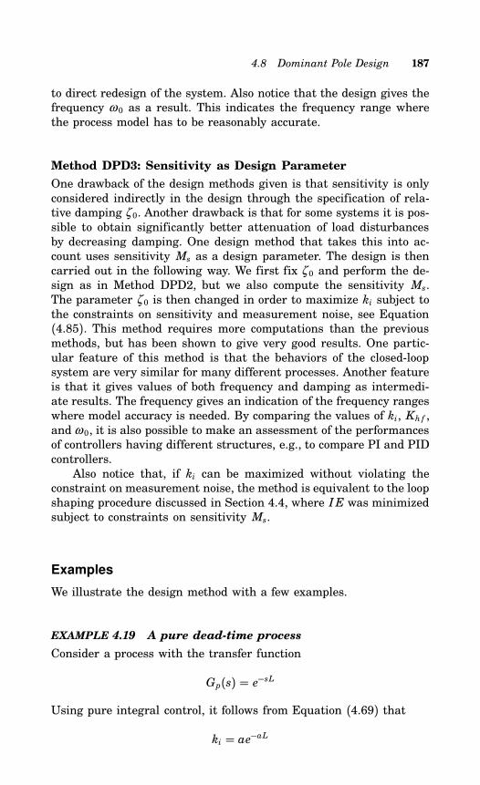
4.8 Dominant Pole Design 187
to direct redesign of the system. Also notice that the design gives thefrequency ω 0 as a result. This indicates the frequency range wherethe process model has to be reasonably accurate.
Method DPD3: Sensitivity as Design Parameter
One drawback of the design methods given is that sensitivity is onlyconsidered indirectly in the design through the specification of rela-tive damping ζ 0. Another drawback is that for some systems it is pos-sible to obtain significantly better attenuation of load disturbancesby decreasing damping. One design method that takes this into ac-count uses sensitivity Ms as a design parameter. The design is thencarried out in the following way. We first fix ζ 0 and perform the de-sign as in Method DPD2, but we also compute the sensitivity Ms.The parameter ζ 0 is then changed in order to maximize ki subject tothe constraints on sensitivity and measurement noise, see Equation(4.85). This method requires more computations than the previousmethods, but has been shown to give very good results. One partic-ular feature of this method is that the behaviors of the closed-loopsystem are very similar for many different processes. Another featureis that it gives values of both frequency and damping as intermedi-ate results. The frequency gives an indication of the frequency rangeswhere model accuracy is needed. By comparing the values of ki, Khf ,and ω 0, it is also possible to make an assessment of the performancesof controllers having different structures, e.g., to compare PI and PIDcontrollers.Also notice that, if ki can be maximized without violating the
constraint on measurement noise, the method is equivalent to the loopshaping procedure discussed in Section 4.4, where IE was minimizedsubject to constraints on sensitivity Ms.
Examples
We illustrate the design method with a few examples.
EXAMPLE 4.19 A pure dead-time process
Consider a process with the transfer function
Gp(s) = e−sL
Using pure integral control, it follows from Equation (4.69) that
ki = ae−aL
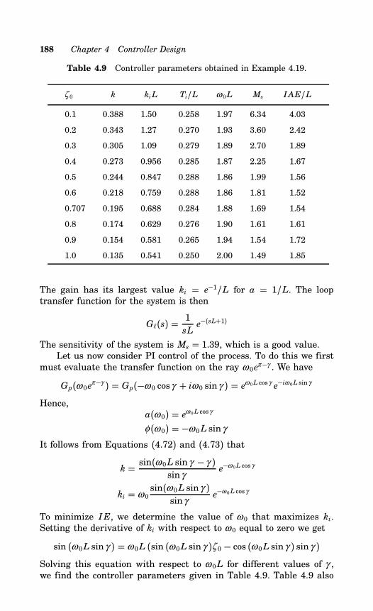
188 Chapter 4 Controller Design
Table 4.9 Controller parameters obtained in Example 4.19.
ζ 0 k kiL Ti/L ω 0L Ms IAE/L
0.1 0.388 1.50 0.258 1.97 6.34 4.03
0.2 0.343 1.27 0.270 1.93 3.60 2.42
0.3 0.305 1.09 0.279 1.89 2.70 1.89
0.4 0.273 0.956 0.285 1.87 2.25 1.67
0.5 0.244 0.847 0.288 1.86 1.99 1.56
0.6 0.218 0.759 0.288 1.86 1.81 1.52
0.707 0.195 0.688 0.284 1.88 1.69 1.54
0.8 0.174 0.629 0.276 1.90 1.61 1.61
0.9 0.154 0.581 0.265 1.94 1.54 1.72
1.0 0.135 0.541 0.250 2.00 1.49 1.85
The gain has its largest value ki = e−1/L for a = 1/L. The looptransfer function for the system is then
G(s) = 1sLe−(sL+1)
The sensitivity of the system is Ms = 1.39, which is a good value.Let us now consider PI control of the process. To do this we first
must evaluate the transfer function on the ray ω 0eπ−γ . We have
Gp(ω 0eπ−γ ) = Gp(−ω 0 cosγ + iω 0 sinγ ) = eω 0L cosγ e−iω 0L sinγ
Hence,a(ω 0) = eω 0L cosγ
φ(ω 0) = −ω 0L sin γ
It follows from Equations (4.72) and (4.73) that
k = sin(ω 0L sin γ − γ )sin γ
e−ω 0L cos γ
ki = ω 0sin(ω 0L sin γ )
sinγe−ω 0L cosγ
To minimize IE, we determine the value of ω 0 that maximizes ki.Setting the derivative of ki with respect to ω 0 equal to zero we get
sin (ω 0L sin γ ) = ω 0L (sin (ω 0L sin γ )ζ 0 − cos (ω 0L sin γ ) sin γ )Solving this equation with respect to ω 0L for different values of γ ,we find the controller parameters given in Table 4.9. Table 4.9 also
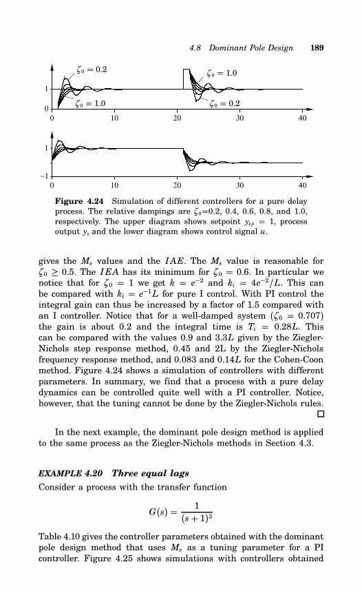
4.8 Dominant Pole Design 189
0 10 20 30 400
1
0 10 20 30 40−1
1
ζ 0 = 0.2
ζ 0 = 1.0
ζ 0 = 1.0
ζ 0 = 0.2
Figure 4.24 Simulation of different controllers for a pure delayprocess. The relative dampings are ζ 0=0.2, 0.4, 0.6, 0.8, and 1.0,respectively. The upper diagram shows setpoint ysp = 1, processoutput y, and the lower diagram shows control signal u.
gives the Ms values and the IAE. The Ms value is reasonable forζ 0 ≥ 0.5. The IEA has its minimum for ζ 0 = 0.6. In particular wenotice that for ζ 0 = 1 we get k = e−2 and ki = 4e−2/L. This canbe compared with ki = e−1L for pure I control. With PI control theintegral gain can thus be increased by a factor of 1.5 compared withan I controller. Notice that for a well-damped system (ζ 0 = 0.707)the gain is about 0.2 and the integral time is Ti = 0.28L. Thiscan be compared with the values 0.9 and 3.3L given by the Ziegler-Nichols step response method, 0.45 and 2L by the Ziegler-Nicholsfrequency response method, and 0.083 and 0.14L for the Cohen-Coonmethod. Figure 4.24 shows a simulation of controllers with differentparameters. In summary, we find that a process with a pure delaydynamics can be controlled quite well with a PI controller. Notice,however, that the tuning cannot be done by the Ziegler-Nichols rules.
In the next example, the dominant pole design method is appliedto the same process as the Ziegler-Nichols methods in Section 4.3.
EXAMPLE 4.20 Three equal lags
Consider a process with the transfer function
G(s) = 1(s+ 1)3
Table 4.10 gives the controller parameters obtained with the dominantpole design method that uses Ms as a tuning parameter for a PIcontroller. Figure 4.25 shows simulations with controllers obtained
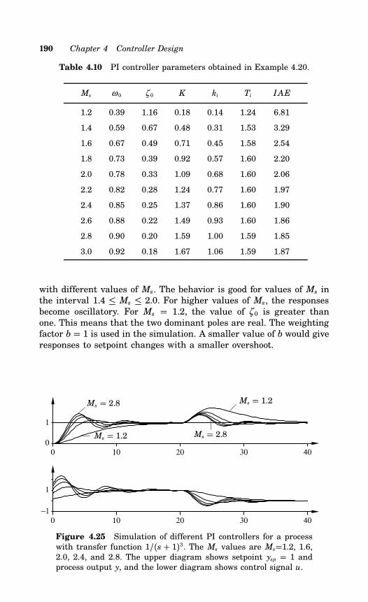
190 Chapter 4 Controller Design
Table 4.10 PI controller parameters obtained in Example 4.20.
Ms ω 0 ζ 0 K ki Ti IAE
1.2 0.39 1.16 0.18 0.14 1.24 6.81
1.4 0.59 0.67 0.48 0.31 1.53 3.29
1.6 0.67 0.49 0.71 0.45 1.58 2.54
1.8 0.73 0.39 0.92 0.57 1.60 2.20
2.0 0.78 0.33 1.09 0.68 1.60 2.06
2.2 0.82 0.28 1.24 0.77 1.60 1.97
2.4 0.85 0.25 1.37 0.86 1.60 1.90
2.6 0.88 0.22 1.49 0.93 1.60 1.86
2.8 0.90 0.20 1.59 1.00 1.59 1.85
3.0 0.92 0.18 1.67 1.06 1.59 1.87
with different values of Ms. The behavior is good for values of Ms inthe interval 1.4 ≤ Ms ≤ 2.0. For higher values of Ms, the responsesbecome oscillatory. For Ms = 1.2, the value of ζ 0 is greater thanone. This means that the two dominant poles are real. The weightingfactor b = 1 is used in the simulation. A smaller value of b would giveresponses to setpoint changes with a smaller overshoot.
0 10 20 30 400
1
0 10 20 30 40−1
1
Ms = 2.8
Ms = 1.2
Ms = 1.2
Ms = 2.8
Figure 4.25 Simulation of different PI controllers for a processwith transfer function 1/(s + 1)3. The Ms values are Ms=1.2, 1.6,2.0, 2.4, and 2.8. The upper diagram shows setpoint ysp = 1 andprocess output y, and the lower diagram shows control signal u.
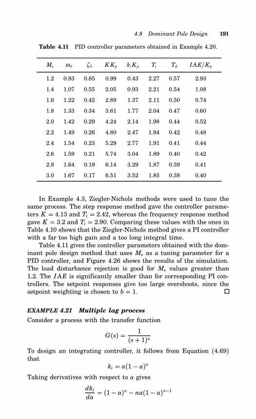
4.8 Dominant Pole Design 191
Table 4.11 PID controller parameters obtained in Example 4.20.
Ms ω 0 ζ 0 KKp kiKp Ti Td IAE/Kp
1.2 0.83 0.85 0.99 0.43 2.27 0.57 2.93
1.4 1.07 0.55 2.05 0.93 2.21 0.54 1.08
1.6 1.22 0.42 2.89 1.37 2.11 0.50 0.74
1.8 1.33 0.34 3.61 1.77 2.04 0.47 0.60
2.0 1.42 0.29 4.24 2.14 1.98 0.44 0.52
2.2 1.49 0.26 4.80 2.47 1.94 0.42 0.48
2.4 1.54 0.23 5.29 2.77 1.91 0.41 0.44
2.6 1.59 0.21 5.74 3.04 1.89 0.40 0.42
2.8 1.64 0.19 6.14 3.29 1.87 0.39 0.41
3.0 1.67 0.17 6.51 3.52 1.85 0.38 0.40
In Example 4.3, Ziegler-Nichols methods were used to tune thesame process. The step response method gave the controller parame-ters K = 4.13 and Ti = 2.42, whereas the frequency response methodgave K = 3.2 and Ti = 2.90. Comparing these values with the ones inTable 4.10 shows that the Ziegler-Nichols method gives a PI controllerwith a far too high gain and a too long integral time.Table 4.11 gives the controller parameters obtained with the dom-
inant pole design method that uses Ms as a tuning parameter for aPID controller, and Figure 4.26 shows the results of the simulation.The load disturbance rejection is good for Ms values greater than1.2. The IAE is significantly smaller than for corresponding PI con-trollers. The setpoint responses give too large overshoots, since thesetpoint weighting is chosen to b = 1.
EXAMPLE 4.21 Multiple lag process
Consider a process with the transfer function
G(s) = 1(s+ 1)n
To design an integrating controller, it follows from Equation (4.69)that
ki = a(1− a)nTaking derivatives with respect to a gives
dki
da= (1− a)n − na(1− a)n−1
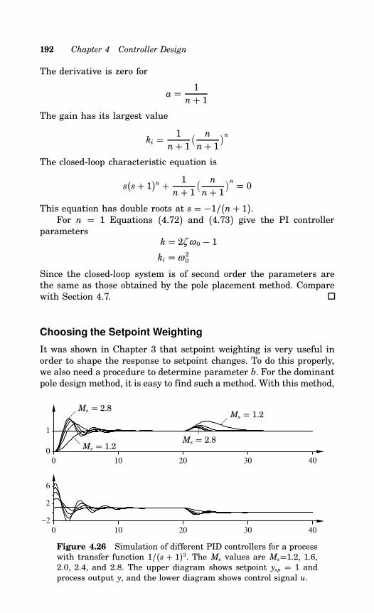
192 Chapter 4 Controller Design
The derivative is zero for
a = 1n+ 1
The gain has its largest value
ki = 1n+ 1
( n
n+ 1)n
The closed-loop characteristic equation is
s(s+ 1)n + 1n+ 1
( n
n+ 1)n = 0
This equation has double roots at s = −1/(n+ 1).For n = 1 Equations (4.72) and (4.73) give the PI controller
parametersk = 2ζ ω 0 − 1ki = ω 20
Since the closed-loop system is of second order the parameters arethe same as those obtained by the pole placement method. Comparewith Section 4.7.
Choosing the Setpoint Weighting
It was shown in Chapter 3 that setpoint weighting is very useful inorder to shape the response to setpoint changes. To do this properly,we also need a procedure to determine parameter b. For the dominantpole design method, it is easy to find such a method. With this method,
0 10 20 30 400
1
0 10 20 30 40−2
2
6
Ms = 2.8
Ms = 1.2
Ms = 1.2
Ms = 2.8
Figure 4.26 Simulation of different PID controllers for a processwith transfer function 1/(s + 1)3. The Ms values are Ms=1.2, 1.6,2.0, 2.4, and 2.8. The upper diagram shows setpoint ysp = 1 andprocess output y, and the lower diagram shows control signal u.
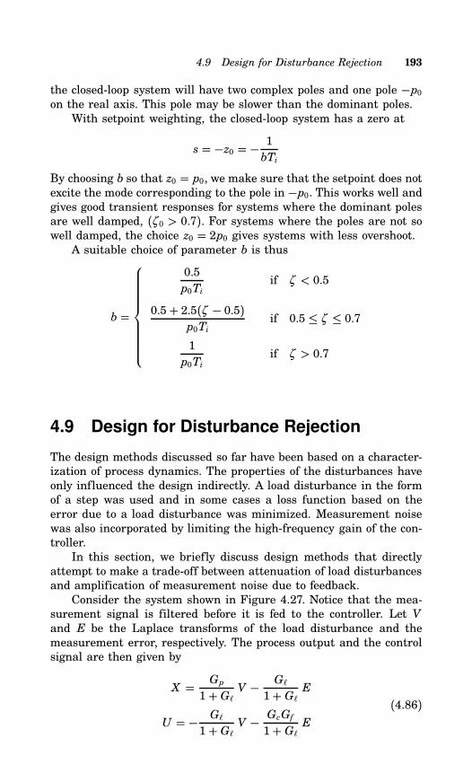
4.9 Design for Disturbance Rejection 193
the closed-loop system will have two complex poles and one pole −p0on the real axis. This pole may be slower than the dominant poles.With setpoint weighting, the closed-loop system has a zero at
s = −z0 = − 1bTi
By choosing b so that z0 = p0, we make sure that the setpoint does notexcite the mode corresponding to the pole in −p0. This works well andgives good transient responses for systems where the dominant polesare well damped, (ζ 0 > 0.7). For systems where the poles are not sowell damped, the choice z0 = 2p0 gives systems with less overshoot.A suitable choice of parameter b is thus
b =
0.5p0Ti
if ζ < 0.5
0.5+ 2.5(ζ − 0.5)p0Ti
if 0.5 ≤ ζ ≤ 0.7
1p0Ti
if ζ > 0.7
4.9 Design for Disturbance Rejection
The design methods discussed so far have been based on a character-ization of process dynamics. The properties of the disturbances haveonly influenced the design indirectly. A load disturbance in the formof a step was used and in some cases a loss function based on theerror due to a load disturbance was minimized. Measurement noisewas also incorporated by limiting the high-frequency gain of the con-troller.In this section, we briefly discuss design methods that directly
attempt to make a trade-off between attenuation of load disturbancesand amplification of measurement noise due to feedback.Consider the system shown in Figure 4.27. Notice that the mea-
surement signal is filtered before it is fed to the controller. Let Vand E be the Laplace transforms of the load disturbance and themeasurement error, respectively. The process output and the controlsignal are then given by
X = Gp
1+ G V −G1+ G E
U = − G1+ G V −
GcGf
1+ G E(4.86)
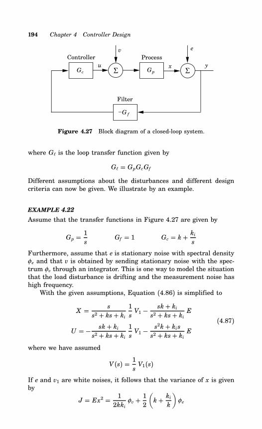
194 Chapter 4 Controller Design
Controller
−
Process
Filter
Σ Σ
v
xu
e
y
G f
Gp Gc
Figure 4.27 Block diagram of a closed-loop system.
where G is the loop transfer function given by
G = GpGcGfDifferent assumptions about the disturbances and different designcriteria can now be given. We illustrate by an example.
EXAMPLE 4.22
Assume that the transfer functions in Figure 4.27 are given by
Gp = 1s
Gf = 1 Gc = k+ kis
Furthermore, assume that e is stationary noise with spectral densityφ e and that v is obtained by sending stationary noise with the spec-trum φv through an integrator. This is one way to model the situationthat the load disturbance is drifting and the measurement noise hashigh frequency.With the given assumptions, Equation (4.86) is simplified to
X = s
s2 + ks+ ki1sV1 − sk+ ki
s2 + ks+ ki E
U = − sk+ kis2 + ks+ ki
1sV1 − s2k+ kis
s2 + ks+ ki E(4.87)
where we have assumed
V (s) = 1sV1(s)
If e and v1 are white noises, it follows that the variance of x is givenby
J = Ex2 = 12kki
φv + 12(k+ ki
k
)φ e
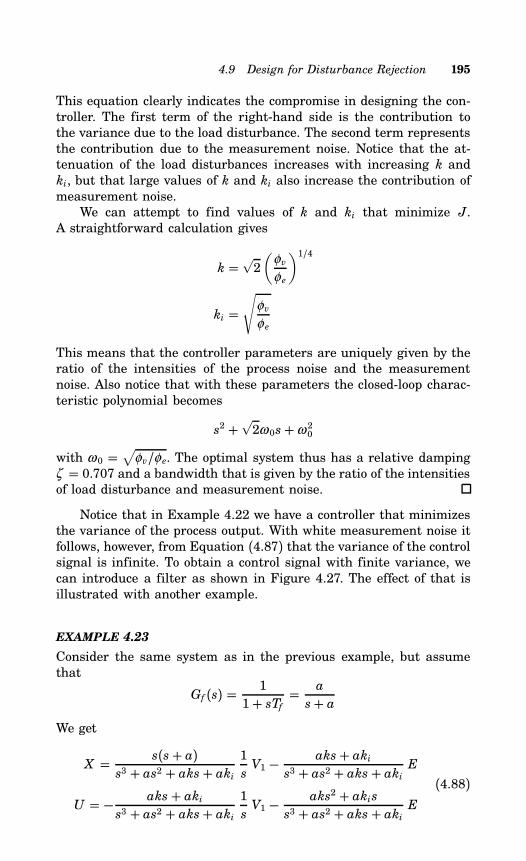
4.9 Design for Disturbance Rejection 195
This equation clearly indicates the compromise in designing the con-troller. The first term of the right-hand side is the contribution tothe variance due to the load disturbance. The second term representsthe contribution due to the measurement noise. Notice that the at-tenuation of the load disturbances increases with increasing k andki, but that large values of k and ki also increase the contribution ofmeasurement noise.We can attempt to find values of k and ki that minimize J.
A straightforward calculation gives
k =√2
(φvφ e
)1/4
ki =√
φvφ e
This means that the controller parameters are uniquely given by theratio of the intensities of the process noise and the measurementnoise. Also notice that with these parameters the closed-loop charac-teristic polynomial becomes
s2 +√2ω 0s+ω 20
with ω 0 =√
φv/φ e. The optimal system thus has a relative dampingζ = 0.707 and a bandwidth that is given by the ratio of the intensitiesof load disturbance and measurement noise.
Notice that in Example 4.22 we have a controller that minimizesthe variance of the process output. With white measurement noise itfollows, however, from Equation (4.87) that the variance of the controlsignal is infinite. To obtain a control signal with finite variance, wecan introduce a filter as shown in Figure 4.27. The effect of that isillustrated with another example.
EXAMPLE 4.23
Consider the same system as in the previous example, but assumethat
Gf (s) = 11+ sTf =
a
s+ aWe get
X = s(s+ a)s3 + as2 + aks+ aki
1sV1 − aks+ aki
s3 + as2 + aks+ aki E
U = − aks+ akis3 + as2 + aks+ aki
1sV1 − aks2 + akis
s3 + as2 + aks+ aki E(4.88)
196 Chapter 4 Controller Design
Assuming that v1 and e are white noise, the variance of the processoutput becomes
J = Ex2 = 12
(ki + a2
aki(ak− ki) φv + aki(k2 + ki)
ki(ak− ki) φ e
)
4.10 Conclusions
The PID controller is by far the most commonly used control strategy.There are many different methods to find suitable parameters of thecontrollers. The methods differ in complexity, flexibility, and in theamount of process knowledge used.There is clearly a need to have several types of tuning methods.
We need simple, easy-to-use, intuitive methods that require littleinformation and that give moderate performance. There is also a needfor sophisticated methods that give the best possible performanceeven if they require more information and more computations.To discuss the methods we must realize that there are many dif-
ferent applications. There are cases where it is desirable to have tightcontrol of the process variable. There are other cases where signifi-cant variations in the process variable is permitted. A typical case issurge tanks where the tank level is allowed to fluctuate considerably,as long as the vessel is neither flooded nor empty.A good tuning method should be based on a rational design
method that considers trade-offs between
• Load disturbance attenuation
• Effects of measurement noise
• Robustness to process variations
• Response to setpoint changes
• Model requirements
• Computational requirements
A tuning method should also be widely applicable. It should containdesign parameters that influence the performance of the closed-loopsystem, and it should admit assessment of the differences in perfor-mance between PI and PID controllers. The method should also makeit possible to judge whether controllers other than PID are more ap-propriate, and it should be applicable to different types of a prioridata. Finally, it is desirable that the method be easy to use. Sincethese requirements are conflicting, it is clear that we need severalmethods.The Ziegler-Nichols method is insufficient in spite of being simple
and widely used. For the more complex models, it is necessary to have
4.11 References 197
more information about the process. This can be obtained by fittingrational functions to frequency responses or by applying system iden-tification techniques. Methods based on cancellation of process poleslike the IMC give simple calculations, but they are not uniformlyapplicable. Methods like the dominant pole design or the frequencyresponse methods are better in this respect, but they are also more de-manding computationally. Since the available computational capacityis expected to increase over the next ten year period, we do not thinkthat this is a major disadvantage.
4.11 References
There is a very large literature on tuning of PID controllers. Good gen-eral sources are the books (Smith, 1972), (Deshpande and Ash, 1981),(Shinskey, 1988), (McMillan, 1983), (Corripio, 1990), and (Suda et al.,1992). The books clearly show the need for a variety of techniques,simple tuning rules, as well as more elaborate procedures that arebased on process modeling, formulation of specifications, and controldesign. Even if simple heuristic rules are used, it is important torealize that they are not a substitute for insight and understanding.Successful controller tuning can not be done without knowledge aboutprocess modeling and control theory. It is also necessary to be awarethat there are many different types of control problems and conse-quently many different design methods. To only use one method is asdangerous as to only believe in empirical tuning rules.Control problems can be specified in many different ways. A good
review of different ways to specify requirements on a control systemis given in (Truxal, 1955), (Maciejowski, 1989), and (Boyd and Bar-ratt, 1991). To formulate specifications it is necessary to be aware ofthe factors that fundamentally limit the performance of a control sys-tem. Simple ways to asses the achievable performance of controllersare given in (Shinskey, 1990), (Shinskey, 1991a), and (Åström, 1991).There are many papers on comparisons of control algorithms and tun-ing methods. The paper (McMillan, 1986) gives much sound advice;other useful papers are (Miller et al., 1967) and (Gerry, 1987).The paper (Ziegler and Nichols, 1942) is the classic work on
controller tuning. An interesting perspective on this paper is givenin an interview with Ziegler, see (Blickley, 1990). The CHR-method,described in (Chien et al., 1952), is a modification of the Ziegler-Nichols method. This is one of the first papers where it is mentionedthat different tuning methods are required for setpoint response andfor load disturbance response. Good response to load disturbances isoften the relevant criteria in process control applications. In spite ofthis, most papers concentrate on the setpoint response. Notice also
198 Chapter 4 Controller Design
that the responses can be tuned independently by having a controllerthat admits a two-degree-of-freedom structure. The usefulness of adesign parameter is also mentioned in the CHR-paper. In spite ofits shortcomings the Ziegler-Nichols method has been the foundationfor many tuning methods, see (Tan and Weber, 1985), (Mantz andTacconi, 1989), and (Hang et al., 1991). Tuning charts were presentedin (Wills, 1962b), (Wills, 1962a), and (Fox, 1979).The loop-shaping methods were inspired by classical control de-
sign methods based on frequency response, see (Truxal, 1955). Appli-cations to PID control are found in (Pessen, 1954), (Habel, 1980),(Chen, 1989), (Yuwana and Seborg, 1982).The analytical tuning method was originally proposed in (New-
ton et al., 1957); a more recent presentation is found in (Boyd andBarratt, 1991). The original papers on the λ-tuning method are(Dahlin, 1968) and (Higham, 1968). The method is sometimes calledthe Dahlin method, see (Deshpande and Ash, 1981). This methodis closely related to the Smith predictor and the internal model con-troller, see (Smith, 1957), (Chien, 1988), (Chien and Fruehauf, 1990),and (Rivera et al., 1986). The PPI controller, which is described in(Hägglund, 1992), and the method given in (Haalman, 1965) are spe-cial cases. The tuning technique developed in (Smith and Murrill,1966), (Pemberton, 1972a), (Pemberton, 1972b), (Smith et al., 1975),(Hwang and Chang, 1987) are also based on the analytical approach.The analytical tuning method gives controllers that cancel poles
and zeros in the transfer function of the process. This leads to lackof observability or controllability. There are severe drawbacks in thisas has been pointed out many times, e.g., in (Shinskey, 1991b) and(Morari and Lee, 1991). The response to load disturbances will bevery sluggish for processes with dominating, long time constants.Many methods for control design are based on optimization tech-
niques. This approach has the advantage that it captures many differ-ent aspects of the design problem. There is also powerful software thatcan be used. A general discussion of the use of optimization for controldesign is found in (Boyd and Barratt, 1991). The papers (Rovira et al.,1969) and (Lopez et al., 1969) give controllers optimized with respectto the criteria ISE, IAE and ITAE. Other applications to PID controlare given in (Hazebroek and van der Waerden, 1950), (Wolfe, 1951),(Oldenburg and Sartorius, 1954), (van der Grinten, 1963a), (Lopezet al., 1967), (Marsili-Libelli, 1981), (Yuwana and Seborg, 1982), (Pat-wardhan et al., 1987), (Wong and Seborg, 1988), (Polonoyi, 1989), and(Zhuang and Atherton, 1991). The methods BO and SO were intro-duced in (Kessler, 1958a) and (Kessler, 1958b). A discussion of thesemethods with many examples are found in (Fröhr, 1967) and (Fröhrand Orttenburger, 1982).Pole placement is a straightforward design method much used
4.11 References 199
in control engineering, see (Truxal, 1955). It has the advantage thatthe closed-loop poles are specified directly. Many other design meth-ods can also be interpreted as pole placement. The papers (Elgerd andStephens, 1959) and (Graham and Lathrop, 1953) show how manyproperties of the closed-loop system can be deduced from the closed-loop poles. This gives good guidance for choosing the suitable closed-loop poles. An early example of pole placement is (Cohen and Coon,1953), (Coon, 1956a), and (Coon, 1956b). It may be difficult to choosedesired closed-loop poles for high-order systems. This is avoided byspecifying only a few poles, as in the dominant pole design methoddescribed in (Persson, 1992), (Persson and Åström, 1992), and (Pers-son and Åström, 1993).There are comparatively few papers on PID controllers that con-
sider the random nature of disturbances. The papers (van der Grin-ten, 1963b), (Goff, 1966a), and (Fertik, 1975) are exceptions.
New Tuning Methods
5.1 Introduction
Many methods for designing PID controllers were presented in Chap-ter 4. From this we can conclude that there are many issues thathave to be taken into account when designing a controller, e.g., loaddisturbance response, measurement noise, setpoint following, modelrequirements, and model uncertainty. It is also clear that there is aneed for a variety of tuning methods; simple techniques that requirelittle process knowledge as well as more elaborate methods that usemore information about the process.In this chapter we use the insight obtained in Chapter 4 to develop
new methods for controller tuning. In Section 5.2 we discuss the keyrequirements on a good design method. In addition to the issuesmentioned above, we consider the choice of design parameters andthe process knowledge required. The method used to develop the newrules is quite straightforward. First we apply a reliable design methodwith the desired characteristics to a large test batch of representativeprocesses. Then we try to correlate the controller parameters obtainedwith simple features that characterize the process dynamics.In Sections 5.3 and 5.4 we present tuning rules that can be viewed
as extensions of the Ziegler-Nichols rules. The main difference is thatwe are using three parameters to characterize process dynamics in-stead of two parameters used by Ziegler and Nichols. It is shown thatthe new methods give substantial improvements in control perfor-mance while retaining much of the simplicity of the Ziegler-Nicholsrules.Methods based on the step response of the process are presented
in Section 5.3. In this case we characterize process dynamics withthe parameters a and L used by Ziegler and Nichols and, in addition,the normalized dead time τ . These parameters are easily determined.The tuning rules obtained give the normal PID parameters and, inaddition, the setpoint weighting.In Section 5.4 we present frequency-domain methods. They are
based on the parameters ultimate gain Ku, ultimate period Tu and
200
5.2 A Spectrum of Tools 201
gain ratio κ . These parameters can be obtained from the conventionalZiegler-Nichols experiment or an experiment with relay tuning com-bined with a determination of the static gain of the process.The methods used in Sections 5.3 and 5.4 are based on approxi-
mate process models. In Section 5.5 we present an efficient method ofcomputing controller gains when the transfer function of the processin known. These results make it possible to judge the advantage inobtaining more process information.In Section 5.6 we explore some consequences of the results of
the previous sections. The closed-loop systems obtained with the newtuning rules may have many poles and zeros. The behavior of theclosed-loop system, however, is dominated by a few poles and zeros.These can be related to the key features of the process. By investi-gating these relations we get interesting insight into the propertiesof the closed-loop system, which can be used to judge achievable per-formance directly from the process features.Examples of using the new tuning rules are given in Section 5.7.
5.2 A Spectrum of Tools
The results of Chapter 4 clearly indicate that a sound tuning methodshould consider many different issues such as load disturbances, mea-surement noise, model requirements, and model accuracy. A good tun-ing method should also have design parameters so that the desiredperformance can be changed easily. Unfortunately, it is not possible tofind a single tuning method that satisfies all requirements. Instead,we develop a spectrum of methods that differ in the effort requiredto use them and in the performance obtained.The wide-spread use of the Ziegler-Nichols methods and its vari-
ants clearly indicates the need for simple methods that use minimalprocess information, but there is also a need for more complex meth-ods that require more effort but, in return, give better control perfor-mance.To develop the simple methods we must first find out if it is at
all possible to obtain reliable tuning rules based on a simple charac-terization of process dynamics. We must also find features that areuseful for characterizing the process dynamics. We have approachedthis in an empirical way by trial and error.We start with a test batch of processes with known transfer func-
tions. Controllers for these processes are then designed using a goodtuning method, e.g., dominant pole design. We then attempt to findprocess features that admit simple description of the controller pa-rameters. The choice of parameters that are useful to characterizeprocess dynamics is guided by the analysis in Chapter 2. After sev-
202 Chapter 5 New Tuning Methods
eral attempts we find that it is possible to obtain reasonable tuningrules based on three parameters, and that the dimension-free param-eters relative dead time τ and relative gain κ are useful.Since the method is based on the parameters κ and τ , it is called
Kappa-Tau tuning, which we also abbreviate as KT tuning. For moreaccurate tuning, it is suggested to use dominant pole design. Thismethod will, however, require more process knowledge.
The Test Batch
The results of an investigation depend critically on the chosen testbatch. We have chosen processes that are representative for the dy-namics of typical industrial processes. The following systems wereused for stable processes.
G1(s) = e−s
(1+ sT)2 T = 0.1, . . . , 10
G2(s) = 1(s+ 1)n n = 3, 4, 8
(5.1)G3(s) = 1
(1+ s)(1+α s)(1+α 2s)(1+α 3s) α = 0.2, 0.5, 0.7
G4(s) = 1−α s
(s+ 1)3 α = 0.1, 0.2, 0.5, 1, 2
To cover processes with integration we also include models obtainedby adding an integrator to the systems listed above.The test batch (5.1) does not include the transfer function
G(s) = Kp e−sL
1+ sT (5.2)
because this model is not representative for typical industrial pro-cesses. Tuning based on the model (5.2) typically give a controllergain that is too high. This is remarkable because tuning rules havetraditionally been based on this model.
Simple Tuning Rules
To obtain the simple tuning rules we use the Ziegler-Nichols rules asa starting point. These rules are based on process data in the form oftwo parameters: a and L for the step-response method, and Tu andKu for the frequency-response method. The properties of the Ziegler-Nichols rules were discussed extensively in Section 4.3. The resultscan be summarized as follows.
5.3 Step-Response Methods 203
A. The responses are too oscillatory.
B. Different tuning rules are required for setpoint response and forload disturbance response.
C. The rules give poor results for systems with long normalized deadtime.
D. There is no tuning parameter.
Drawback A is easy to deal with. It is sufficient to modify the pa-rameters in the tables. Item B can be dealt with by tuning for loaddisturbances and using setpoint weighting to obtain the desired set-point response. Item C is more difficult to deal with because it isnecessary to have more process information. A first step is to char-acterize the process by three parameters instead of two. It turns outthat this gives a substantial improvement.As a tuning parameter we use the maximum sensitivity Ms. Recall
that this parameter is defined as
Ms = maxω
∣∣∣∣ 11+ Gp(iω )Gc(iω )
∣∣∣∣where Gc(s) is the controller transfer function and Gp(s) the processtransfer function. The parameter also has a nice geometrical interpre-tation in the Nyquist diagram. The shortest distance from the criticalpoint −1 to the Nyquist curve of GpGc is 1/Ms. This admits a directinterpretation as a robustness measure, because it tells how muchthe process can change without causing instability. Typical values ofMs are in the range of 1.2 to 2. Larger values of Ms give systems thatare faster but less robust. It is also useful that the range to consideris not too large.
5.3 Step-Response Methods
In this section we describe simple tuning rules based on step-responsedata. The need for such techniques are clear in an historical perspec-tive. A simple tuning method of this type is useful for manual tuningand it can also be incorporated into automatic tuners. It turns outthat it is possible to obtain substantial improvements compared toother approaches at the cost of a modest increase in complexity.
Stable Processes
First we consider the case when the processes are stable. Processdynamics are characterized by three parameters: the static gain Kp,the apparent lag T , and the apparent dead time L. In Chapter 2 we
204 Chapter 5 New Tuning Methods
discussed different ways to determine these parameters experimen-tally. In that section we also found that it is difficult to determinemore than three parameters from a step response. There is some ar-bitrariness in the determination of L and T . Here we determine Las the intersection of the tangent with the steepest slope with thetime axis. Parameter T is determined as the time when the step re-sponse reaches 63% of its final value. An alternative is to determinethe average residence time, Tar , by the method of moments and todetermine T from
T = Tar − LTo present the results it is convenient to reparameterize the process.Guided by the Ziegler-Nichols formula we use the parameter
a = Kp LT
instead of Kp and the relative dead time
τ = L
L + T =L
Tar
instead of T .
Integrating Processes
Parameters a and L can be determined from a step-response exper-iment for processes with integration. Since the process is not stableit will, however, not reach a steady state. The initial part of the re-sponse can be determined, but the experiment has to be interruptedafter some time.The relative dead time τ is zero for processes with integration.
It can thus be attempted to use the formulas derived for stable pro-cesses with τ = 0. It is, however, useful to base the tuning on moreinformation about the initial part of the step response. This can beobtained from the impulse response of the system, which can be ap-proximated by the pulse response if the pulse is sufficiently short. Ifthe transfer function of the process is G(s), we have
G(s) = 1sH(s)
where H(s) is a stable transfer function. A step-response experimentperformed on H(s) is equivalent to a pulse-response experiment per-formed on G(s). Thus, we can determine the steady-state gain K ′p andthe average residence time T ′ar for the transfer function H(s) usingthe methods discussed in Chapter 2. It can be shown that
a = K ′pT ′ar = K ′p(L′ + T ′)L = T ′ar = L′ + T ′
5.3 Step-Response Methods 205
Parameters a and L are therefore easy to obtain from the pulseexperiment. The normalized dead time τ ′, associated with transferfunction H(s), can be used as an additional parameter. Tuning rulesbased on a, L, and τ ′ can be developed for processes with integration.They are similar to the rules for stable processes.In the old literature on controller tuning the expression “processes
with self-regulation” was used to describe stable processes and “pro-cesses without self-regulation” was used to describe processes withintegration. It is interesting to observe that these classes always weretreated separately in classical papers on controller tuning.
Normalization of Controller Parameters
The PI controller has three parameters: the gain K , the integrationtime Ti, and the setpoint weighting b. It is convenient to representthese parameters in dimension-free form by suitable normalization.The normalized controller gain is aK , and the normalized integrationtime Ti/L. This is the same normalization used in the Ziegler-Nicholsrules. (Compare with Section 4.3.) In some cases the integration timewill be normalized by T instead of L. Notice that parameter T is notdefined for processes with integration. This is the reason why it isbetter to base the tuning on L than on T .
The Method
An empirical method is used to find the new tuning rules. Controllerparameters are computed for the different processes in the test batch,using dominant pole design. We then attempt to find relations be-tween the normalized controller parameters and the normalized pro-cess parameters. This is done by plotting the normalized controllerparameters as a function of normalized dead time τ . For example, weinvestigate whether the normalized controller gain can be expressedas
aK = f (τ )and analogous expressions for the other parameters. It turns out thatit is indeed possible to find approximations of this type. The functionsobtained can be well approximated by functions having the form
f (τ ) = a0ea1τ+a2τ 2 (5.3)Many other functions can also be used.
PI Control for Stable Processes
The simplified tuning rules for PI controllers are treated first. Fig-ure 5.1 shows the normalized controller parameters as a function of
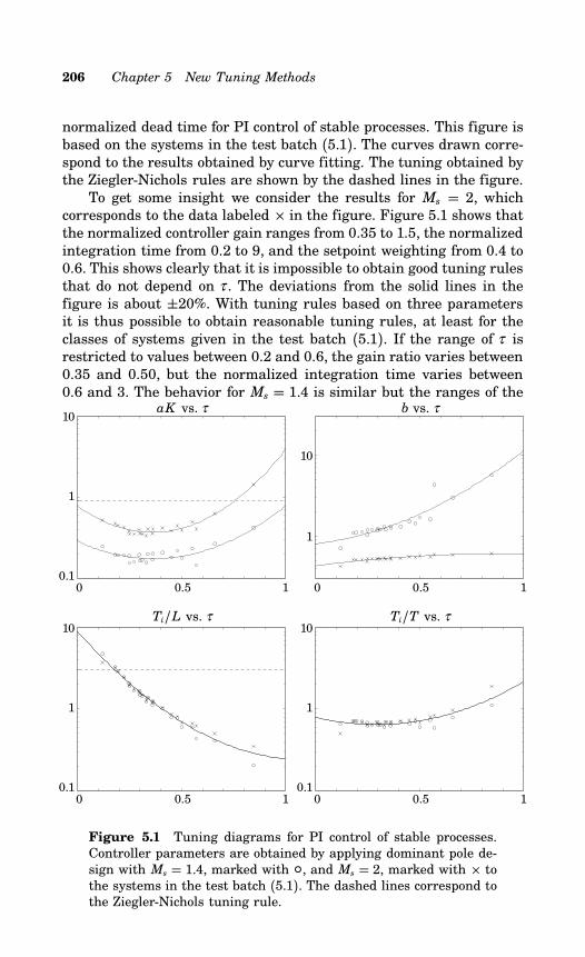
206 Chapter 5 New Tuning Methods
normalized dead time for PI control of stable processes. This figure isbased on the systems in the test batch (5.1). The curves drawn corre-spond to the results obtained by curve fitting. The tuning obtained bythe Ziegler-Nichols rules are shown by the dashed lines in the figure.To get some insight we consider the results for Ms = 2, which
corresponds to the data labeled in the figure. Figure 5.1 shows thatthe normalized controller gain ranges from 0.35 to 1.5, the normalizedintegration time from 0.2 to 9, and the setpoint weighting from 0.4 to0.6. This shows clearly that it is impossible to obtain good tuning rulesthat do not depend on τ . The deviations from the solid lines in thefigure is about ±20%. With tuning rules based on three parametersit is thus possible to obtain reasonable tuning rules, at least for theclasses of systems given in the test batch (5.1). If the range of τ isrestricted to values between 0.2 and 0.6, the gain ratio varies between0.35 and 0.50, but the normalized integration time varies between0.6 and 3. The behavior for Ms = 1.4 is similar but the ranges of the
aK vs. τ
0 0.5 10.1
1
10b vs. τ
0 0.5 1
1
10
Ti/L vs. τ
0 0.5 10.1
1
10Ti/T vs. τ
0 0.5 10.1
1
10
Figure 5.1 Tuning diagrams for PI control of stable processes.Controller parameters are obtained by applying dominant pole de-sign with Ms = 1.4, marked with , and Ms = 2, marked with tothe systems in the test batch (5.1). The dashed lines correspond tothe Ziegler-Nichols tuning rule.
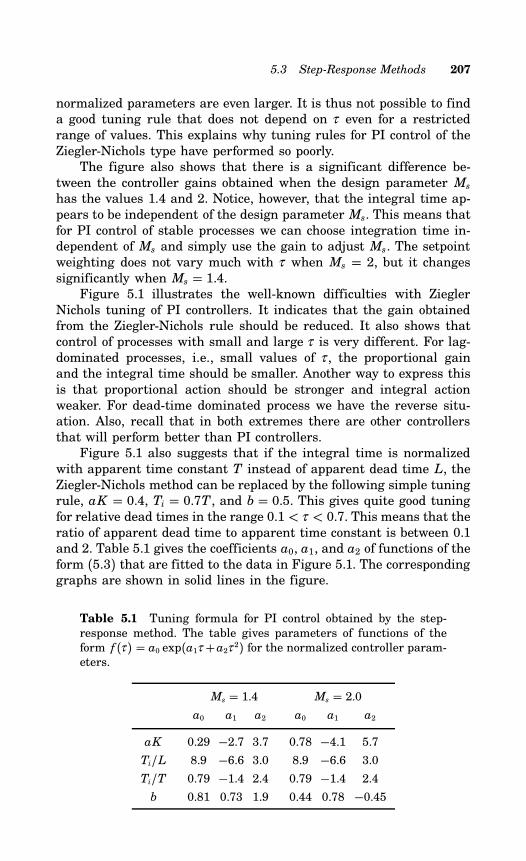
5.3 Step-Response Methods 207
normalized parameters are even larger. It is thus not possible to finda good tuning rule that does not depend on τ even for a restrictedrange of values. This explains why tuning rules for PI control of theZiegler-Nichols type have performed so poorly.The figure also shows that there is a significant difference be-
tween the controller gains obtained when the design parameter Mshas the values 1.4 and 2. Notice, however, that the integral time ap-pears to be independent of the design parameter Ms. This means thatfor PI control of stable processes we can choose integration time in-dependent of Ms and simply use the gain to adjust Ms. The setpointweighting does not vary much with τ when Ms = 2, but it changessignificantly when Ms = 1.4.Figure 5.1 illustrates the well-known difficulties with Ziegler
Nichols tuning of PI controllers. It indicates that the gain obtainedfrom the Ziegler-Nichols rule should be reduced. It also shows thatcontrol of processes with small and large τ is very different. For lag-dominated processes, i.e., small values of τ , the proportional gainand the integral time should be smaller. Another way to express thisis that proportional action should be stronger and integral actionweaker. For dead-time dominated process we have the reverse situ-ation. Also, recall that in both extremes there are other controllersthat will perform better than PI controllers.Figure 5.1 also suggests that if the integral time is normalized
with apparent time constant T instead of apparent dead time L, theZiegler-Nichols method can be replaced by the following simple tuningrule, aK = 0.4, Ti = 0.7T , and b = 0.5. This gives quite good tuningfor relative dead times in the range 0.1 < τ < 0.7. This means that theratio of apparent dead time to apparent time constant is between 0.1and 2. Table 5.1 gives the coefficients a0, a1, and a2 of functions of theform (5.3) that are fitted to the data in Figure 5.1. The correspondinggraphs are shown in solid lines in the figure.
Table 5.1 Tuning formula for PI control obtained by the step-response method. The table gives parameters of functions of theform f (τ ) = a0 exp(a1τ +a2τ 2) for the normalized controller param-eters.
Ms = 1.4 Ms = 2.0a0 a1 a2 a0 a1 a2
aK 0.29 −2.7 3.7 0.78 −4.1 5.7
Ti/L 8.9 −6.6 3.0 8.9 −6.6 3.0
Ti/T 0.79 −1.4 2.4 0.79 −1.4 2.4
b 0.81 0.73 1.9 0.44 0.78 −0.45
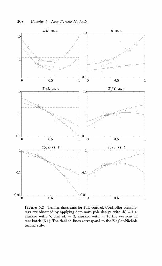
208 Chapter 5 New Tuning Methods
aK vs. τ
0 0.5 1
1
10
b vs. τ
0 0.5 10.1
1
10
Ti/L vs. τ
0 0.5 10.1
1
10Ti/T vs. τ
0 0.5 10.1
1
10
Td/L vs. τ
0 0.5 10.01
0.1
1Td/T vs. τ
0 0.5 10.01
0.1
1
Figure 5.2 Tuning diagrams for PID control. Controller parame-ters are obtained by applying dominant pole design with Ms = 1.4,marked with , and Ms = 2, marked with , to the systems intest batch (5.1). The dashed lines correspond to the Ziegler-Nicholstuning rule.
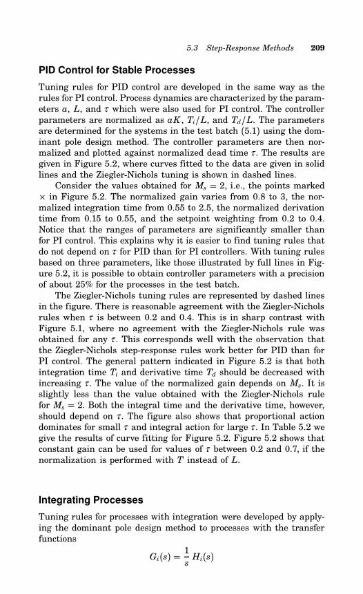
5.3 Step-Response Methods 209
PID Control for Stable Processes
Tuning rules for PID control are developed in the same way as therules for PI control. Process dynamics are characterized by the param-eters a, L, and τ which were also used for PI control. The controllerparameters are normalized as aK , Ti/L, and Td/L. The parametersare determined for the systems in the test batch (5.1) using the dom-inant pole design method. The controller parameters are then nor-malized and plotted against normalized dead time τ . The results aregiven in Figure 5.2, where curves fitted to the data are given in solidlines and the Ziegler-Nichols tuning is shown in dashed lines.Consider the values obtained for Ms = 2, i.e., the points marked
in Figure 5.2. The normalized gain varies from 0.8 to 3, the nor-malized integration time from 0.55 to 2.5, the normalized derivationtime from 0.15 to 0.55, and the setpoint weighting from 0.2 to 0.4.Notice that the ranges of parameters are significantly smaller thanfor PI control. This explains why it is easier to find tuning rules thatdo not depend on τ for PID than for PI controllers. With tuning rulesbased on three parameters, like those illustrated by full lines in Fig-ure 5.2, it is possible to obtain controller parameters with a precisionof about 25% for the processes in the test batch.The Ziegler-Nichols tuning rules are represented by dashed lines
in the figure. There is reasonable agreement with the Ziegler-Nicholsrules when τ is between 0.2 and 0.4. This is in sharp contrast withFigure 5.1, where no agreement with the Ziegler-Nichols rule wasobtained for any τ . This corresponds well with the observation thatthe Ziegler-Nichols step-response rules work better for PID than forPI control. The general pattern indicated in Figure 5.2 is that bothintegration time Ti and derivative time Td should be decreased withincreasing τ . The value of the normalized gain depends on Ms. It isslightly less than the value obtained with the Ziegler-Nichols rulefor Ms = 2. Both the integral time and the derivative time, however,should depend on τ . The figure also shows that proportional actiondominates for small τ and integral action for large τ . In Table 5.2 wegive the results of curve fitting for Figure 5.2. Figure 5.2 shows thatconstant gain can be used for values of τ between 0.2 and 0.7, if thenormalization is performed with T instead of L.
Integrating Processes
Tuning rules for processes with integration were developed by apply-ing the dominant pole design method to processes with the transferfunctions
Gi(s) = 1sHi(s)
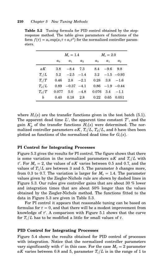
210 Chapter 5 New Tuning Methods
Table 5.2 Tuning formula for PID control obtained by the step-response method. The table gives parameters of functions of theform f (τ ) = a0 exp(a1τ +a2τ 2) for the normalized controller param-eters.
Ms = 1.4 Ms = 2.0a0 a1 a2 a0 a1 a2
aK 3.8 −8.4 7.3 8.4 −9.6 9.8
Ti/L 5.2 −2.5 −1.4 3.2 −1.5 −0.93Ti/T 0.46 2.8 −2.1 0.28 3.8 −1.6Td/L 0.89 −0.37 −4.1 0.86 −1.9 −0.44Td/T 0.077 5.0 −4.8 0.076 3.4 −1.1b 0.40 0.18 2.8 0.22 0.65 0.051
where Hi(s) are the transfer functions given in the test batch (5.1).The apparent dead time L′, the apparent time constant T ′, and thegain K ′p of the transfer functions Hi(s) were determined. The nor-malized controller parameters aK , Ti/L, Td/L, and b have then beenplotted as functions of the normalized dead time for Gi(s).
PI Control for Integrating Processes
Figure 5.3 gives the results for PI control. The figure shows that thereis some variation in the normalized parameters aK and Ti/L withτ ′. For Ms = 2, the values of aK varies between 0.5 and 0.7, and thevalues of Ti/L are between 3 and 5. The parameter b changes more,from 0.3 to 0.7. The variation is larger for Ms = 1.4. The parametervalues given by the Ziegler-Nichols rule are shown by dashed lines inFigure 5.3. Our rules give controller gains that are about 30 % lowerand integration times that are about 50% longer than the valuesobtained by the Ziegler-Nichols method. The functions fitted to thedata in Figure 5.3 are given in Table 5.3.For PI control it appears that reasonable tuning can be based on
formulas for τ = 0, and that there will be a modest improvement fromknowledge of τ ′. A comparison with Figure 5.1 shows that the curvefor Ti/L has to be modified a little for small values of τ .
PID Control for Integrating Processes
Figure 5.4 shows the results obtained for PID control of processeswith integration. Notice that the normalized controller parametersvary significantly with τ ′ in this case. For the case Ms = 2 parameteraK varies between 0.8 and 5, parameter Ti/L is in the range of 1 to
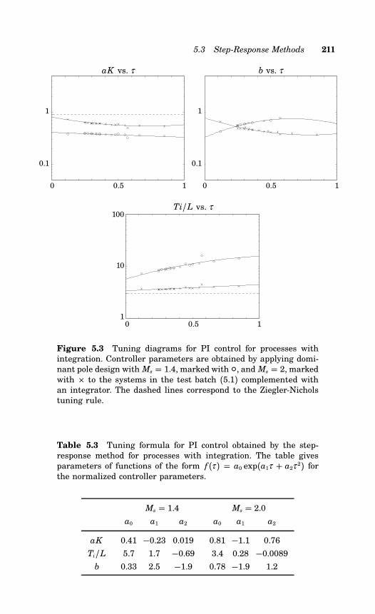
5.3 Step-Response Methods 211
aK vs. τ
0 0.5 1
0.1
1
b vs. τ
0 0.5 1
0.1
1
Ti/L vs. τ
0 0.5 11
10
100
Figure 5.3 Tuning diagrams for PI control for processes withintegration. Controller parameters are obtained by applying domi-nant pole design with Ms = 1.4, marked with , and Ms = 2, markedwith to the systems in the test batch (5.1) complemented withan integrator. The dashed lines correspond to the Ziegler-Nicholstuning rule.
Table 5.3 Tuning formula for PI control obtained by the step-response method for processes with integration. The table givesparameters of functions of the form f (τ ) = a0 exp(a1τ + a2τ 2) forthe normalized controller parameters.
Ms = 1.4 Ms = 2.0a0 a1 a2 a0 a1 a2
aK 0.41 −0.23 0.019 0.81 −1.1 0.76
Ti/L 5.7 1.7 −0.69 3.4 0.28 −0.0089b 0.33 2.5 −1.9 0.78 −1.9 1.2
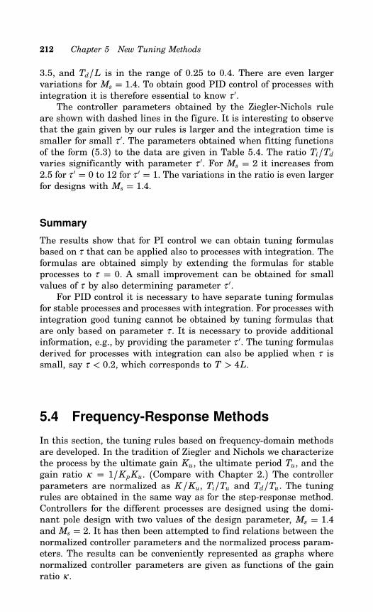
212 Chapter 5 New Tuning Methods
3.5, and Td/L is in the range of 0.25 to 0.4. There are even largervariations for Ms = 1.4. To obtain good PID control of processes withintegration it is therefore essential to know τ ′.The controller parameters obtained by the Ziegler-Nichols rule
are shown with dashed lines in the figure. It is interesting to observethat the gain given by our rules is larger and the integration time issmaller for small τ ′. The parameters obtained when fitting functionsof the form (5.3) to the data are given in Table 5.4. The ratio Ti/Tdvaries significantly with parameter τ ′. For Ms = 2 it increases from2.5 for τ ′ = 0 to 12 for τ ′ = 1. The variations in the ratio is even largerfor designs with Ms = 1.4.
Summary
The results show that for PI control we can obtain tuning formulasbased on τ that can be applied also to processes with integration. Theformulas are obtained simply by extending the formulas for stableprocesses to τ = 0. A small improvement can be obtained for smallvalues of τ by also determining parameter τ ′.For PID control it is necessary to have separate tuning formulas
for stable processes and processes with integration. For processes withintegration good tuning cannot be obtained by tuning formulas thatare only based on parameter τ . It is necessary to provide additionalinformation, e.g., by providing the parameter τ ′. The tuning formulasderived for processes with integration can also be applied when τ issmall, say τ < 0.2, which corresponds to T > 4L.
5.4 Frequency-Response Methods
In this section, the tuning rules based on frequency-domain methodsare developed. In the tradition of Ziegler and Nichols we characterizethe process by the ultimate gain Ku, the ultimate period Tu, and thegain ratio κ = 1/KpKu. (Compare with Chapter 2.) The controllerparameters are normalized as K/Ku, Ti/Tu and Td/Tu. The tuningrules are obtained in the same way as for the step-response method.Controllers for the different processes are designed using the domi-nant pole design with two values of the design parameter, Ms = 1.4and Ms = 2. It has then been attempted to find relations between thenormalized controller parameters and the normalized process param-eters. The results can be conveniently represented as graphs wherenormalized controller parameters are given as functions of the gainratio κ .
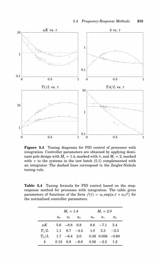
5.4 Frequency-Response Methods 213
aK vs. τ
0 0.5 10.1
1
10b vs. τ
0 0.5 1
0.1
1
Ti/L vs. τ
0 0.5 1
1
10
Td/L vs. τ
0 0.5 10.1
1
10
Figure 5.4 Tuning diagrams for PID control of processes withintegration. Controller parameters are obtained by applying domi-nant pole design with Ms = 1.4, marked with , and Ms = 2, markedwith to the systems in the test batch (5.1) complemented withan integrator. The dashed lines correspond to the Ziegler-Nicholstuning rule.
Table 5.4 Tuning formula for PID control based on the step-response method for processes with integration. The table givesparameters of functions of the form f (τ ) = a0 exp(a1τ + a2τ 2) forthe normalized controller parameters.
Ms = 1.4 Ms = 2.0a0 a1 a2 a0 a1 a2
aK 5.6 −8.8 6.8 8.6 −7.1 5.4
Ti/L 1.1 6.7 −4.4 1.0 3.3 −2.3Td/L 1.7 −6.4 2.0 0.38 0.056 −0.60b 0.12 6.9 −6.6 0.56 −2.2 1.2
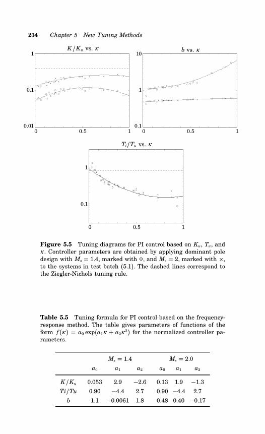
214 Chapter 5 New Tuning Methods
K/Ku vs. κ
0 0.5 10.01
0.1
1b vs. κ
0 0.5 10.1
1
10
Ti/Tu vs. κ
0 0.5 1
0.1
1
Figure 5.5 Tuning diagrams for PI control based on Ku, Tu, andκ . Controller parameters are obtained by applying dominant poledesign with Ms = 1.4, marked with , and Ms = 2, marked with ,to the systems in test batch (5.1). The dashed lines correspond tothe Ziegler-Nichols tuning rule.
Table 5.5 Tuning formula for PI control based on the frequency-response method. The table gives parameters of functions of theform f (κ ) = a0 exp(a1κ + a2κ 2) for the normalized controller pa-rameters.
Ms = 1.4 Ms = 2.0a0 a1 a2 a0 a1 a2
K/Ku 0.053 2.9 −2.6 0.13 1.9 −1.3Ti/Tu 0.90 −4.4 2.7 0.90 −4.4 2.7
b 1.1 −0.0061 1.8 0.48 0.40 −0.17
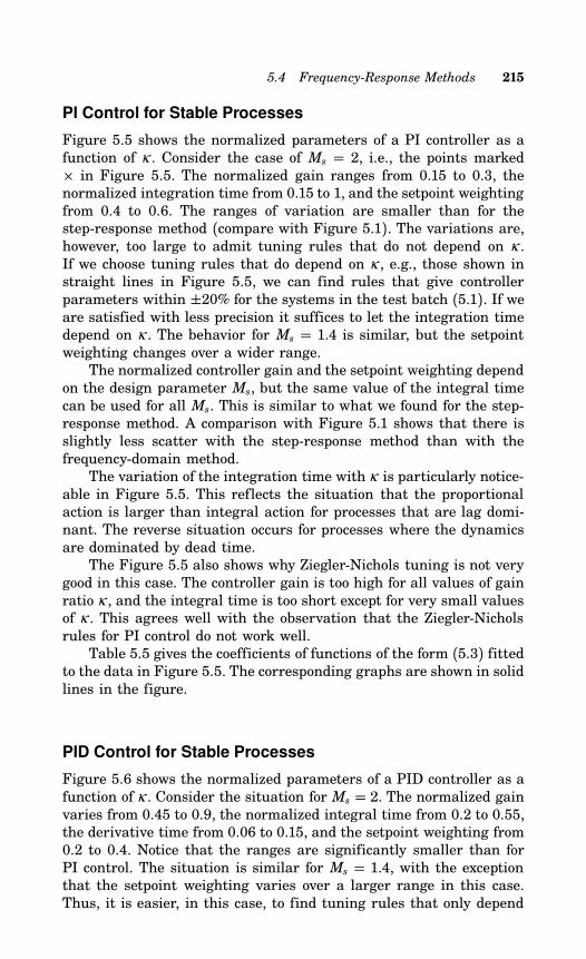
5.4 Frequency-Response Methods 215
PI Control for Stable Processes
Figure 5.5 shows the normalized parameters of a PI controller as afunction of κ . Consider the case of Ms = 2, i.e., the points marked in Figure 5.5. The normalized gain ranges from 0.15 to 0.3, thenormalized integration time from 0.15 to 1, and the setpoint weightingfrom 0.4 to 0.6. The ranges of variation are smaller than for thestep-response method (compare with Figure 5.1). The variations are,however, too large to admit tuning rules that do not depend on κ .If we choose tuning rules that do depend on κ , e.g., those shown instraight lines in Figure 5.5, we can find rules that give controllerparameters within ±20% for the systems in the test batch (5.1). If weare satisfied with less precision it suffices to let the integration timedepend on κ . The behavior for Ms = 1.4 is similar, but the setpointweighting changes over a wider range.The normalized controller gain and the setpoint weighting depend
on the design parameter Ms, but the same value of the integral timecan be used for all Ms. This is similar to what we found for the step-response method. A comparison with Figure 5.1 shows that there isslightly less scatter with the step-response method than with thefrequency-domain method.The variation of the integration time with κ is particularly notice-
able in Figure 5.5. This reflects the situation that the proportionalaction is larger than integral action for processes that are lag domi-nant. The reverse situation occurs for processes where the dynamicsare dominated by dead time.The Figure 5.5 also shows why Ziegler-Nichols tuning is not very
good in this case. The controller gain is too high for all values of gainratio κ , and the integral time is too short except for very small valuesof κ . This agrees well with the observation that the Ziegler-Nicholsrules for PI control do not work well.Table 5.5 gives the coefficients of functions of the form (5.3) fitted
to the data in Figure 5.5. The corresponding graphs are shown in solidlines in the figure.
PID Control for Stable Processes
Figure 5.6 shows the normalized parameters of a PID controller as afunction of κ . Consider the situation for Ms = 2. The normalized gainvaries from 0.45 to 0.9, the normalized integral time from 0.2 to 0.55,the derivative time from 0.06 to 0.15, and the setpoint weighting from0.2 to 0.4. Notice that the ranges are significantly smaller than forPI control. The situation is similar for Ms = 1.4, with the exceptionthat the setpoint weighting varies over a larger range in this case.Thus, it is easier, in this case, to find tuning rules that only depend
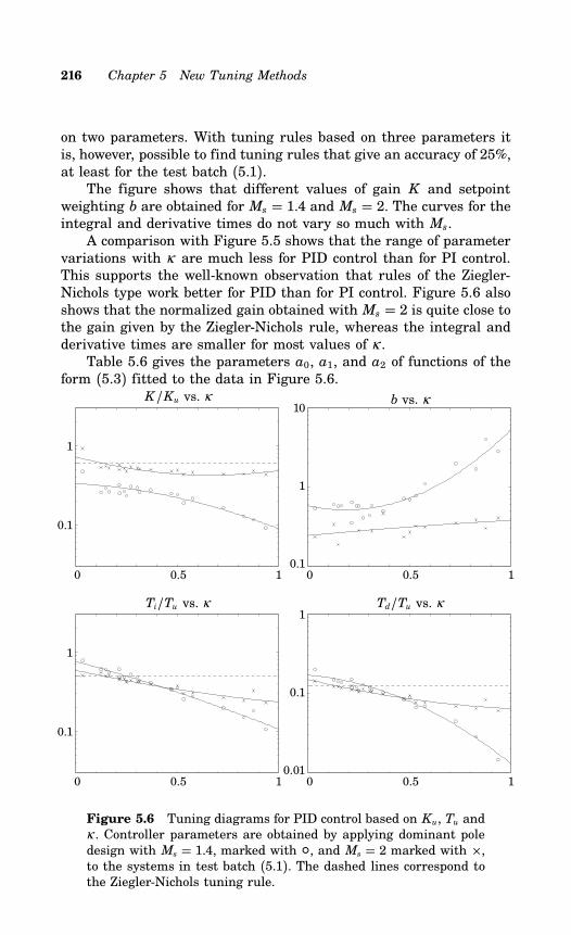
216 Chapter 5 New Tuning Methods
on two parameters. With tuning rules based on three parameters itis, however, possible to find tuning rules that give an accuracy of 25%,at least for the test batch (5.1).The figure shows that different values of gain K and setpoint
weighting b are obtained for Ms = 1.4 and Ms = 2. The curves for theintegral and derivative times do not vary so much with Ms.A comparison with Figure 5.5 shows that the range of parameter
variations with κ are much less for PID control than for PI control.This supports the well-known observation that rules of the Ziegler-Nichols type work better for PID than for PI control. Figure 5.6 alsoshows that the normalized gain obtained with Ms = 2 is quite close tothe gain given by the Ziegler-Nichols rule, whereas the integral andderivative times are smaller for most values of κ .Table 5.6 gives the parameters a0, a1, and a2 of functions of the
form (5.3) fitted to the data in Figure 5.6.K/Ku vs. κ
0 0.5 1
0.1
1
b vs. κ
0 0.5 10.1
1
10
Ti/Tu vs. κ
0 0.5 1
0.1
1
Td/Tu vs. κ
0 0.5 10.01
0.1
1
Figure 5.6 Tuning diagrams for PID control based on Ku, Tu andκ . Controller parameters are obtained by applying dominant poledesign with Ms = 1.4, marked with , and Ms = 2 marked with ,to the systems in test batch (5.1). The dashed lines correspond tothe Ziegler-Nichols tuning rule.
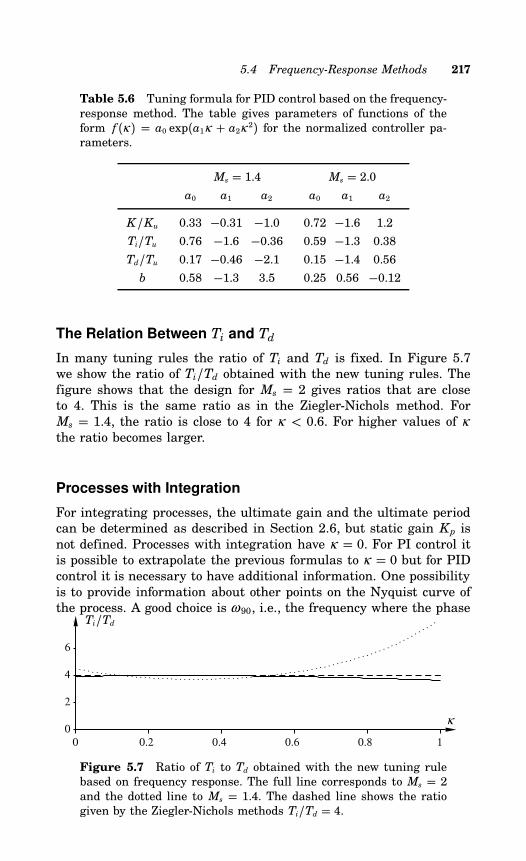
5.4 Frequency-Response Methods 217
Table 5.6 Tuning formula for PID control based on the frequency-response method. The table gives parameters of functions of theform f (κ ) = a0 exp(a1κ + a2κ 2) for the normalized controller pa-rameters.
Ms = 1.4 Ms = 2.0a0 a1 a2 a0 a1 a2
K/Ku 0.33 −0.31 −1.0 0.72 −1.6 1.2
Ti/Tu 0.76 −1.6 −0.36 0.59 −1.3 0.38
Td/Tu 0.17 −0.46 −2.1 0.15 −1.4 0.56
b 0.58 −1.3 3.5 0.25 0.56 −0.12
The Relation Between Ti and Td
In many tuning rules the ratio of Ti and Td is fixed. In Figure 5.7we show the ratio of Ti/Td obtained with the new tuning rules. Thefigure shows that the design for Ms = 2 gives ratios that are closeto 4. This is the same ratio as in the Ziegler-Nichols method. ForMs = 1.4, the ratio is close to 4 for κ < 0.6. For higher values of κthe ratio becomes larger.
Processes with Integration
For integrating processes, the ultimate gain and the ultimate periodcan be determined as described in Section 2.6, but static gain Kp isnot defined. Processes with integration have κ = 0. For PI control itis possible to extrapolate the previous formulas to κ = 0 but for PIDcontrol it is necessary to have additional information. One possibilityis to provide information about other points on the Nyquist curve ofthe process. A good choice is ω 90, i.e., the frequency where the phase
0 0.2 0.4 0.6 0.8 10
2
4
6
Ti/Td
κ
Figure 5.7 Ratio of Ti to Td obtained with the new tuning rulebased on frequency response. The full line corresponds to Ms = 2and the dotted line to Ms = 1.4. The dashed line shows the ratiogiven by the Ziegler-Nichols methods Ti/Td = 4.
218 Chapter 5 New Tuning Methods
lag is 90.
5.5 Complete Process Knowledge
The methods presented in Sections 5.3 and 5.4 are approximate meth-ods based on partial knowledge of the process. These methods aresufficient in many cases. There are, however, situations where moreaccuracy is required. This can be achieved either by on-line refine-ment or by using a more accurate model. There are many empiricalrules for on-line tuning that can be refined further by selecting dif-ferent rule sets depending on the values of τ or κ .A more accurate model can be obtained by using system iden-
tification. This will typically give a model in the form of a pulsetransfer function. This model can be transformed into an ordinarytransfer function in several different ways. Since the tuning methodsare based on the transfer function of the process, it is attractive touse frequency response techniques. The multifrequency method is atechnique where a signal that is a sum of sinusoids is chosen as theinput. The phases of the sinusoids are chosen so that the amplitudeof the signal is minimized. The frequencies chosen can be based onthe knowledge of the ultimate frequency ωu. In this way it is possibleto obtain the value of the transfer function for several frequenciesin one test. A transfer function can then be fitted to the data, andthe dominant pole design technique can then be used. In this sec-tion we present alternative methods of performing the computationsrequired for dominant pole design. An alternative to this is to deter-mine a pulse transfer function by applying the system identificationmethods discussed in Section 2.7 and to develop a design procedurethat is based on the pulse transfer function. Such a method can beobtained using ideas similar to those discussed in this chapter.
PI Control
Consider a process with the transfer function G(s). Let the PI con-troller be parameterized as
Gc(s) = k+ kis
(5.4)
In this particular case the design problem can be formulated as fol-lows. Find the parameters k and ki such that ki is as large as possibleand so that the robustness constraint
1+ G(iω ) = a(k, ki,ω ) ≥ m0 (5.5)
5.5 Complete Process Knowledge 219
where G = G(s)Gc(s) is the loop transfer function. The problem is aconstrained optimization problem that, unfortunately, is not convex.To solve it we use an iterative method with good initial conditions.The idea of the algorithm is to evaluate the function
m(k, ki) = minω∈Ωa(k, ki,ω ) = m0 (5.6)
for several values of the controller parameters and then to determinethe value of k, which maximizes ki subject to the constraint.Determination of the function m requires minimization with re-
spect to ω . This is done by a simple search over the interval Ω =[ω 1,ω 2].The function m can be locally approximated by
m(k, ki) = a+ b0ki + b1k+ 12(c0k
2i + 2c1kki + c2k2
) (5.7)
Maximizing ki with respect to k subject to the constraint (5.6) gives
b1 + c1ki + c2k = 0 (5.8)
This gives the following relation between k and ki:
k = −b1 + c1kic2
(5.9)
Inserting this into Equation (5.7) and using the condition m(k, ki) =m0 gives
A0k2i + 2A1ki + A2 = 0 (5.10)
where
A0 = c0 − c21
c2
A1 = b0 − b1c1c2
A2 = 2(a0 −m0) − b21
c2
Solving Equation (5.10) gives
ki =−A1 ±
√A21 − A0A2A0
(5.11)
Having obtained ki the value of k is then given by Equation (5.9).Parameters for PID controllers can be determined in a similar
way.
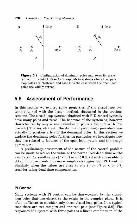
220 Chapter 5 New Tuning Methods
Re sRe s
Im s Im s
ω o ω o
− po − po− zo − zo
A B
Figure 5.8 Configuration of dominant poles and zeros for a sys-tem with PI control. Case A corresponds to systems where the open-loop poles are clustered and case B is the case when the open-looppoles are widely spread.
5.6 Assessment of Performance
In this section we explore some properties of the closed-loop sys-tems obtained with the design methods discussed in the previoussections. The closed-loop systems obtained with PID control typicallyhave many poles and zeros. The behavior of the system is, however,characterized by only a small number of poles. (Compare with Fig-ure 4.4.) The key idea with the dominant pole design procedure wasactually to position a few of the dominant poles. In this section weexplore the dominant poles further. In particular we investigate howthey are related to features of the open loop system and the designparameters.A preliminary assessment of the nature of the control problem
can be made based on the value of the normalized dead time or thegain ratio. For small values (τ < 0.1 or κ < 0.06) it is often possible toobtain improved control by more complex strategies than PID control.Similarly when the values are close to one (τ > 0.7 or κ > 0.7)consider using dead-time compensation.
PI Control
Many systems with PI control can be characterized by the closed-loop poles that are closest to the origin in the complex plane. It isoften sufficient to consider only three closed-loop poles. In a typicalcase there are two complex and one real pole (see Figure 5.8). Theresponses of a system with three poles is a linear combination of the
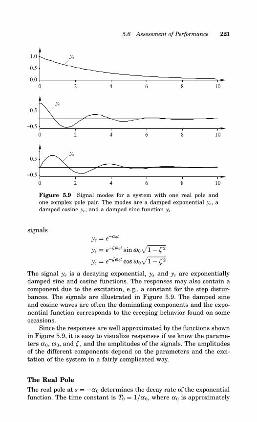
5.6 Assessment of Performance 221
0 2 4 6 8 100.0
0.5
1.0
0 2 4 6 8 10
−0.5
0.5
0 2 4 6 8 10
−0.5
0.5
ye
yc
ys
Figure 5.9 Signal modes for a system with one real pole andone complex pole pair. The modes are a damped exponential ye, adamped cosine yc, and a damped sine function ys.
signalsye = e−α 0t
ys = e−ζ ω 0t sinω 0√1− ζ 2
yc = e−ζ ω 0t cosω 0√1− ζ 2
The signal ye is a decaying exponential, ys and yc are exponentiallydamped sine and cosine functions. The responses may also contain acomponent due to the excitation, e.g., a constant for the step distur-bances. The signals are illustrated in Figure 5.9. The damped sineand cosine waves are often the dominating components and the expo-nential function corresponds to the creeping behavior found on someoccasions.Since the responses are well approximated by the functions shown
in Figure 5.9, it is easy to visualize responses if we know the parame-ters α 0, ω 0, and ζ , and the amplitudes of the signals. The amplitudesof the different components depend on the parameters and the exci-tation of the system in a fairly complicated way.
The Real Pole
The real pole at s = −α 0 determines the decay rate of the exponentialfunction. The time constant is T0 = 1/α 0, where α 0 is approximately
222 Chapter 5 New Tuning Methods
equal to 1/Ti. This explains the sluggish response obtained when Tiis too large, compare with Figure 5.9.For processes, where the open-loop poles are clustered together,
the configuration of the poles is as shown in Figure 5.8A. The polelocated in −α 0 is thus to the right of the zero −z0 = −1/Ti. Forsystems where the open-loop poles are widely separated, the poleconfiguration is as shown in Figure 5.8B, where the real pole is tothe left of the zero −z0. The cases can approximately be separatedthrough the inequality
T0 > 2(L +
n∑k=1Tk
)= 2(Tar − T0) (5.12)
where T0 is the time constant associated with the slowest pole (α 0),Tk are the time constants associated with the remaining poles, andTar is the average residence time (see Section 2.4). The inequality isobtained by analyzing the root locus of the system.
Complex Poles
The damped sine and cosine modes are determined by parameters ω 0and ζ . The period of the oscillation is
Tp = 2π
ω 0√1− ζ 2
and the ratio of two successive peaks are
d = e−2πζ /√1−ζ 2
(Compare with Section 4.2.) Knowing parameters ω 0 and ζ , it is thuseasy to visualize the shape of the mode.If the parameters of the controller are determined by the dom-
inant pole design, we can determine how ω 0, ζ , and α 0 depend onthe system and the specifications. In this way it is possible to relatethe properties of the closed-loop system directly to the features of theprocess.To find good relations we use the normalized quantities ω 0L andα 0Ti. The relative damping is dimension free by itself. Figure 5.10shows the relations obtained for the test batch (5.1). For Ms = 2 thequantity ω 0L ranges from 0.5 to 1.5; ζ ranges from 0.3 to 0.6, andα 0Ti from 0.8 to 1.2. The value of ω 0L is less than one for small τor κ and larger than one for large values. The variation with τ orκ is larger for Ms = 1.4 than for Ms = 2. For Ms = 1.4 the relativedamping depends strongly on τ or κ ; it is larger than one for largevalues of τ or κ . This means that the closed-loop system has threereal poles. The value of α 0Ti is smaller than one in most cases. This
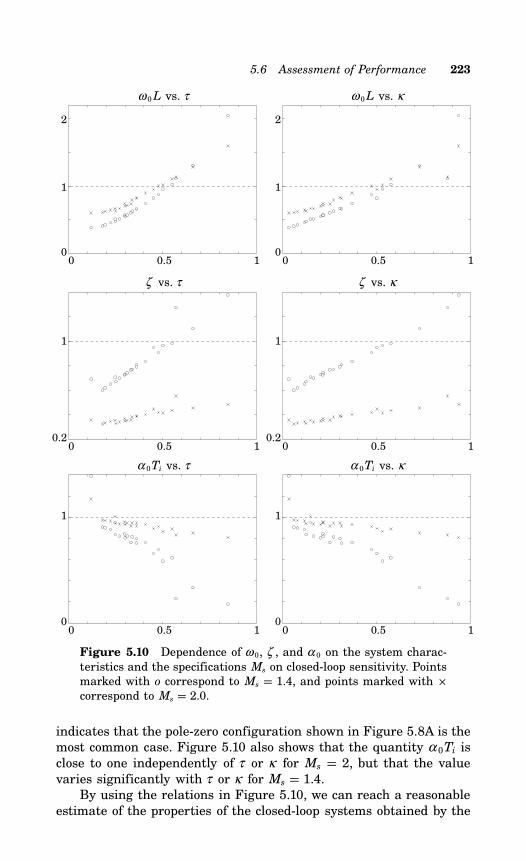
5.6 Assessment of Performance 223
ω 0L vs. τ
0 0.5 10
1
2
ω 0L vs. κ
0 0.5 10
1
2
ζ vs. τ
0 0.5 10.2
1
ζ vs. κ
0 0.5 10.2
1
α 0Ti vs. τ
0 0.5 10
1
α 0Ti vs. κ
0 0.5 10
1
Figure 5.10 Dependence of ω 0, ζ , and α 0 on the system charac-teristics and the specifications Ms on closed-loop sensitivity. Pointsmarked with o correspond to Ms = 1.4, and points marked with correspond to Ms = 2.0.
indicates that the pole-zero configuration shown in Figure 5.8A is themost common case. Figure 5.10 also shows that the quantity α 0Ti isclose to one independently of τ or κ for Ms = 2, but that the valuevaries significantly with τ or κ for Ms = 1.4.By using the relations in Figure 5.10, we can reach a reasonable
estimate of the properties of the closed-loop systems obtained by the
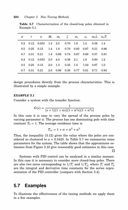
224 Chapter 5 New Tuning Methods
Table 5.7 Characterization of the closed-loop poles obtained inExample 5.1.
α τ κ Ms ω 0 ζ α 0 z0 ω 0L α 0Ti
0.2 0.12 0.033 1.4 2.5 0.70 1.9 1.4 0.38 1.4
0.5 0.25 0.15 1.4 1.0 0.70 0.93 0.97 0.51 0.96
0.7 0.31 0.21 1.4 0.69 0.74 0.67 0.68 0.57 0.81
0.2 0.12 0.033 2.0 4.0 0.36 2.1 1.8 0.60 1.2
0.5 0.25 0.15 2.0 1.3 0.35 1.0 1.02 0.67 1.0
0.7 0.31 0.21 2.0 0.86 0.36 0.77 0.81 0.71 0.94
design procedures directly from the process characteristics. This isillustrated by a simple example.
EXAMPLE 5.1
Consider a system with the transfer function.
G(s) = 1(s+ 1)(1+α s)(1+α 2s)(1+α 3s)
In this case it is easy to vary the spread of the process poles byvarying parameter α . The process has one dominating pole with timeconstant T0 = 1. The average residence time is
Tar = 1+α +α 2 +α 3
Thus, the inequality (5.12) gives the value where the poles are con-sidered as clustered to a = 0.3425. In Table 5.7 we summarize someparameters for the system. The table shows that the approximate es-timates from Figure 5.10 give reasonably good estimates in this case.
Systems with PID control can be analyzed in a similar manner.In this case it is necessary to consider more closed-loop poles. Thereare also two zeros corresponding to 1/T ′i and 1/T ′d, where T ′i and T ′dare the integral and derivative time constants for the series repre-sentation of the PID controller (compare with Section 3.4).
5.7 Examples
To illustrate the effectiveness of the tuning methods we apply themin a few examples.
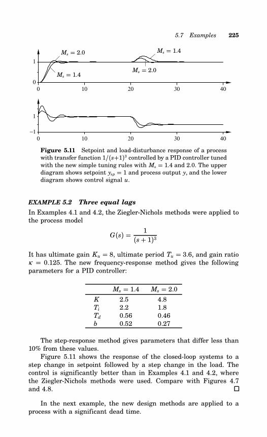
5.7 Examples 225
0 10 20 30 400
1
0 10 20 30 40−1
1
Ms = 2.0
Ms = 1.4
Ms = 1.4
Ms = 2.0
Figure 5.11 Setpoint and load-disturbance response of a processwith transfer function 1/(s+1)3 controlled by a PID controller tunedwith the new simple tuning rules with Ms = 1.4 and 2.0. The upperdiagram shows setpoint ysp = 1 and process output y, and the lowerdiagram shows control signal u.
EXAMPLE 5.2 Three equal lags
In Examples 4.1 and 4.2, the Ziegler-Nichols methods were applied tothe process model
G(s) = 1(s+ 1)3
It has ultimate gain Ku = 8, ultimate period Tu = 3.6, and gain ratioκ = 0.125. The new frequency-response method gives the followingparameters for a PID controller:
Ms = 1.4 Ms = 2.0K 2.5 4.8Ti 2.2 1.8Td 0.56 0.46b 0.52 0.27
The step-response method gives parameters that differ less than10% from these values.Figure 5.11 shows the response of the closed-loop systems to a
step change in setpoint followed by a step change in the load. Thecontrol is significantly better than in Examples 4.1 and 4.2, wherethe Ziegler-Nichols methods were used. Compare with Figures 4.7and 4.8.
In the next example, the new design methods are applied to aprocess with a significant dead time.
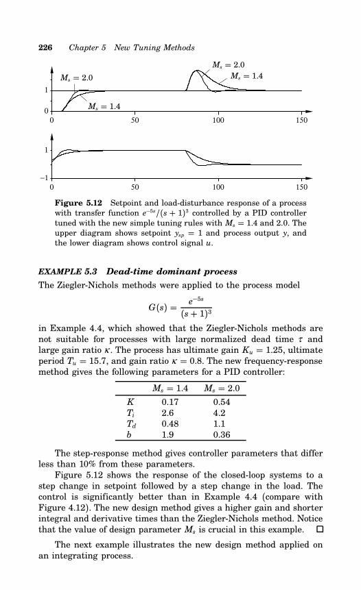
226 Chapter 5 New Tuning Methods
0 50 100 1500
1
0 50 100 150−1
1
Ms = 2.0
Ms = 1.4
Ms = 2.0Ms = 1.4
Figure 5.12 Setpoint and load-disturbance response of a processwith transfer function e−5s/(s + 1)3 controlled by a PID controllertuned with the new simple tuning rules with Ms = 1.4 and 2.0. Theupper diagram shows setpoint ysp = 1 and process output y, andthe lower diagram shows control signal u.
EXAMPLE 5.3 Dead-time dominant process
The Ziegler-Nichols methods were applied to the process model
G(s) = e−5s
(s+ 1)3in Example 4.4, which showed that the Ziegler-Nichols methods arenot suitable for processes with large normalized dead time τ andlarge gain ratio κ . The process has ultimate gain Ku = 1.25, ultimateperiod Tu = 15.7, and gain ratio κ = 0.8. The new frequency-responsemethod gives the following parameters for a PID controller:
Ms = 1.4 Ms = 2.0K 0.17 0.54Ti 2.6 4.2Td 0.48 1.1b 1.9 0.36
The step-response method gives controller parameters that differless than 10% from these parameters.Figure 5.12 shows the response of the closed-loop systems to a
step change in setpoint followed by a step change in the load. Thecontrol is significantly better than in Example 4.4 (compare withFigure 4.12). The new design method gives a higher gain and shorterintegral and derivative times than the Ziegler-Nichols method. Noticethat the value of design parameter Ms is crucial in this example.
The next example illustrates the new design method applied onan integrating process.
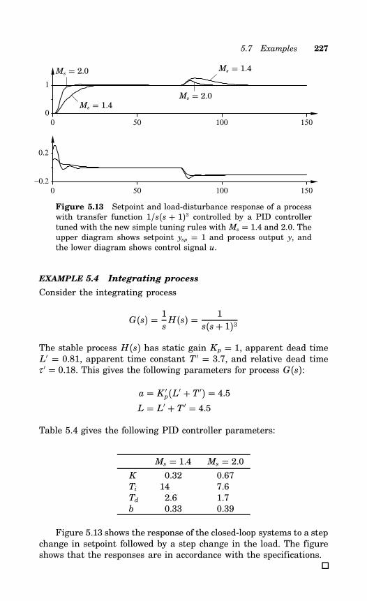
5.7 Examples 227
0 50 100 1500
1
0 50 100 150−0.2
0.2
Ms = 2.0
Ms = 1.4Ms = 2.0
Ms = 1.4
Figure 5.13 Setpoint and load-disturbance response of a processwith transfer function 1/s(s + 1)3 controlled by a PID controllertuned with the new simple tuning rules with Ms = 1.4 and 2.0. Theupper diagram shows setpoint ysp = 1 and process output y, andthe lower diagram shows control signal u.
EXAMPLE 5.4 Integrating process
Consider the integrating process
G(s) = 1sH(s) = 1
s(s+ 1)3
The stable process H(s) has static gain Kp = 1, apparent dead timeL′ = 0.81, apparent time constant T ′ = 3.7, and relative dead timeτ ′ = 0.18. This gives the following parameters for process G(s):
a = K ′p(L′ + T ′) = 4.5L = L′ + T ′ = 4.5
Table 5.4 gives the following PID controller parameters:
Ms = 1.4 Ms = 2.0K 0.32 0.67Ti 14 7.6Td 2.6 1.7b 0.33 0.39
Figure 5.13 shows the response of the closed-loop systems to a stepchange in setpoint followed by a step change in the load. The figureshows that the responses are in accordance with the specifications.
228 Chapter 5 New Tuning Methods
5.8 Conclusions
In this section we have developed new methods for tuning PID con-trollers. The methods are based on specifications in terms of rejectionof load disturbances and measurement noise, sensitivity to model-ing errors, and setpoint response. Rejection of load disturbances isthe primary design criterion that is optimized by minimizing the in-tegrated error. Modeling errors are captured by requiring that themaximum sensitivity be less than a specified value Ms. This valueis a design variable that can be chosen by the user. Reasonable vari-ables range from Ms = 1.4 to Ms = 2. The standard value is Ms = 2,but smaller values can be chosen if responses without overshoot aredesired.The method is based on the dominant pole design, wich requires
that the transfer function of the process is known. The methods de-scribed in this section require the same parameters as the Ziegler-Nichols methods, and, in addition, κ for the frequency domain methodand τ for the step response method. The tuning method, therefore, iscalled the Kappa-Tau method or the KT method for short. The tuningmethod works for processes that are typically encountered in processcontrol. The KT-tuning techniques may be viewed as a generalizationof the Ziegler-Nichols method.For the step-response method the process is characterized by the
apparent dead time, the apparent time constant, and the static gain.For the frequency-domain method, the parameters ultimate gain, ul-timate period, and static gain characterize the process. The tuningrules are conveniently expressed using the normalized variables gainratio κ and normalized dead time τ .The KT method gives insight into the shortcomings of the Ziegler-
Nichols rules. First, they avoid the poor damping obtained with theZiegler-Nichols rule. Secondly, they give good tuning also for processeswith long dead time. The results also show that knowledge aboutthe gain ratio or the normalized dead time is required for tuninga PI controller. For PID control with small values of κ and τ , e.g.,processes with integration, it is shown that improved tuning requiresadditional knowledge. This can be obtained from the impulse responseof the system. The results admit assessment of the performance thatcan be achieved with the new tuning rules based on simple processcharacteristics.
5.9 References
The results given in this chapter were motivated by the desire toobtain tuning rules that are simple and significantly better than the
5.9 References 229
Ziegler-Nichols rules. The chapter is based on the ideas in (Hanget al., 1991), (Åström et al., 1992). The idea to use dimension-freeparameters was used there. Notice, however, that the definitions ofnormalized dead time τ , and gain ratio κ are different. The reasonfor making changes is that it is helpful to have parameters thatrange from zero to one. Much more primitive tuning procedures wereused in the previous work. The dominant pole design, which is thebasis for the work, is given in (Persson, 1992), see also (Persson andÅström, 1992), (Persson and Åström, 1993), and (Persson, 1992). Theidea of using dimension-free quantities for performance assessment isdiscussed in (Åström, 1991). They are also useful for an autonomouscontroller, see (Åström, 1992).
Automatic Tuningand Adaptation
6.1 Introduction
By combining the methods for determination of process dynamics (de-scribed in Chapter 2) with the methods for computing the parametersof a PID controller (described in Chapter 4), methods for automatictuning of PID controllers can be obtained. By automatic tuning (orauto-tuning) we mean a method where the controller is tuned auto-matically on demand from a user. Typically the user will either pusha button or send a command to the controller. An automatic tuningprocedure consists of three steps:
• Generation of a process disturbance.
• Evaluation of the disturbance response.
• Calculation of controller parameters.
This is the same procedure that an experienced operator uses whentuning a controller manually. The process must be disturbed in someway in order to determine the process dynamics. This can be donein many ways, e.g., by adding steps, pulses, or sinusoids to the pro-cess input. The evaluation of the disturbance response may include adetermination of a process model or a simple characterization of theresponse.Industrial experience has clearly indicated that automatic tuning
is a highly desirable and useful feature. Automatic tuning is some-times called tuning on demand or one-shot tuning. Commercial PIDcontrollers with automatic tuning facilities have only been available
since the beginning of the eighties. There are several reasons for this.The recent development of microelectronics has made it possible toincorporate the additional program code needed for the automatictuning at a reasonable cost. The interest in automatic tuning at uni-versities is also quite new. Most of the research effort has been devotedto the related, but more difficult, problem of adaptive control.
230
6.1 Introduction 231
Automatic tuning can also be performed using external equip-ment. These devices are connected to the control loop only duringthe tuning phase. When the tuning experiment is finished, the prod-ucts suggest controller parameters. Since these products are supposedto work together with controllers from different manufacturers, theymust be provided with quite a lot of information about the controllerin order to give an appropriate parameter suggestion. The informationrequired includes controller structure (standard, series, or parallelform), sampling rate, filter time constants, and units of the differentcontroller parameters (gain or proportional band, minutes or seconds,time or repeats/time). The fact that PID controllers are parameter-ized in so many ways creates unnecessary difficulties.Tuning facilities are also starting to appear in the distributed
control systems. In this case it is possible to have a very powerfulinteraction of the user because of the graphics and computationalcapabilities available in the system.Even when automatic tuning devices are used, it is important to
obtain a certain amount of process knowledge. This is discussed inthe next section. Automatic tuning is only one way to use the adap-tive technique. Section 6.3 gives an overview of several adaptive tech-niques, as well as a discussion about the use of these techniques.The automatic tuning approaches can be divided into two categories,namely model-based approaches and rule-based approaches. In themodel-based approaches, a model of the process is obtained explicitly,and the tuning is based on this model. Section 6.4 treats approacheswere the model is obtained from transient response experiments, fre-quency response experiments, and parameter estimation. In the rule-based approaches, no explicit process model is obtained. The tuning isbased instead on rules similar to those rules that an experienced op-erator uses to tune the controller manually. The rule-based approachis treated in Section 6.5.Some industrial products with adaptive facilities are presented
in Section 6.6. Four single-station controllers are presented: FoxboroEXACT (760/761), Alfa Laval Automation ECA400, Honeywell UDC6000, and Yokogawa SLPC-181 and 281. Three tuning packages to beused within DCS systems, Fisher-Rosemount Intelligent Tuner andGain Scheduler, Honeywell Looptune, and ABB DCS Tuner are alsopresented, as well as the process analyzer Techmation Protuner.Adaptive techniques are closely related to diagnosis procedures.
Section 6.7 gives an overview of both manual and automatic on-linediagnosis procedures. The chapter ends with conclusions and refer-ences in Sections 6.8 and 6.9
232 Chapter 6 Automatic Tuning and Adaptation
6.2 Process Knowledge
In this chapter we will discuss several methods for automatic tuning.Before going into details we must remark that poor behavior of acontrol loop can not always be corrected by tuning the controller. It isabsolutely necessary to understand the reason for the poor behavior.The process may be poorly designed so that there are long dead
times, long time constants, nonlinearities, and inverse responses. Sen-sors and actuators may be poorly placed or badly mounted, and theymay have bad dynamics. Typical examples are thermocouples withheavy casings that make their response slow, or on-off valve motorswith long travel time. Valves may be oversized so that they only actover a small region. The sensor span may be too wide so that poorresolution is obtained, or it may also have excessive sensor noise. Theprocedure of investigating whether a process is well designed from acontrol point of view is called loop auditing.There may also be failure and wear in the process equipment.
Valves may have excessive stiction. There may be backlash due towear. Sensors may drift and change their properties because of con-tamination.If a control loop is behaving unsatisfactorily, it is essential that
we first determine the reason for this before tuning is attempted. Itwould, of course, be highly desirable to have aids for the process engi-neer to do the diagnosis. Automatic tuning may actually do the wrongthing if it is not applied with care. For example, consider a controlloop that oscillates because of friction in the actuator. Practically alltuning devices will attempt to stabilize the oscillation by reducing thecontroller gain. This will only increase the period of the oscillation!Remember—no amount of so called “intelligence” in equipment
can replace real process knowledge.
6.3 Adaptive Techniques
Techniques for automatic tuning grew out of research in adaptive con-trol. Adaptation was originally developed to deal with processes withcharacteristics that were changing with time or with operating con-ditions. Practically all adaptive techniques can be used for automatictuning. The adaptive controller is simply run until the parametershave converged and the parameters are then kept constant. The draw-back with this approach is that adaptive controllers may require priorinformation. There are many special techniques that can be used forthis purpose. Industrial experience has shown that this is probablythe most useful application of adaptive techniques. Gain scheduling isalso a very effective technique to cope with processes that change their
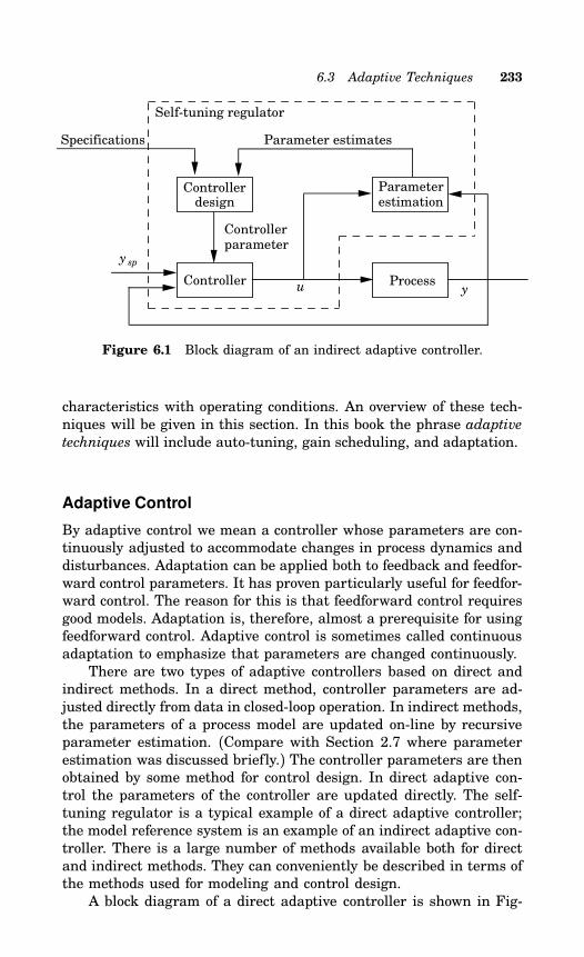
6.3 Adaptive Techniques 233
designController
Controller Process
Controllerparameter
Parameter estimatesSpecifications
Self-tuning regulator
yu
y sp
Parameterestimation
Figure 6.1 Block diagram of an indirect adaptive controller.
characteristics with operating conditions. An overview of these tech-niques will be given in this section. In this book the phrase adaptivetechniques will include auto-tuning, gain scheduling, and adaptation.
Adaptive Control
By adaptive control we mean a controller whose parameters are con-tinuously adjusted to accommodate changes in process dynamics anddisturbances. Adaptation can be applied both to feedback and feedfor-ward control parameters. It has proven particularly useful for feedfor-ward control. The reason for this is that feedforward control requiresgood models. Adaptation is, therefore, almost a prerequisite for usingfeedforward control. Adaptive control is sometimes called continuousadaptation to emphasize that parameters are changed continuously.There are two types of adaptive controllers based on direct and
indirect methods. In a direct method, controller parameters are ad-justed directly from data in closed-loop operation. In indirect methods,the parameters of a process model are updated on-line by recursiveparameter estimation. (Compare with Section 2.7 where parameterestimation was discussed briefly.) The controller parameters are thenobtained by some method for control design. In direct adaptive con-trol the parameters of the controller are updated directly. The self-tuning regulator is a typical example of a direct adaptive controller;the model reference system is an example of an indirect adaptive con-troller. There is a large number of methods available both for directand indirect methods. They can conveniently be described in terms ofthe methods used for modeling and control design.A block diagram of a direct adaptive controller is shown in Fig-
234 Chapter 6 Automatic Tuning and Adaptation
ure 6.1. There is a parameter estimator that determines the param-eters of the model based on observations of process inputs and out-puts. There is also a design block that computes controller parametersfrom the model parameters. If the system is operated as a tuner, theprocess is excited by an input signal. The parameters can either beestimated recursively or in batch mode. Controller parameters arecomputed and the controller is commissioned. If the system is oper-ated as an adaptive controller, parameters are computed recursivelyand controller parameters are updated when new parameter valuesare obtained.
Automatic Tuning
By automatic tuning (or auto-tuning) we mean a method where a con-troller is tuned automatically on demand from a user. Typically theuser will either push a button or send a command to the controller.Industrial experience has clearly indicated that this is a highly desir-able and useful feature. Automatic tuning is sometimes called tuningon demand or one-shot tuning. Auto-tuning can be built into the con-trollers. Practically all controllers can benefit from tools for automatictuning. This will drastically simplify the use of controllers. Single loopcontrollers and distributed systems for process control are importantapplication areas. Most of these controllers are of the PID type. Thisis a vast application area because there are millions of controllers ofthis type in use. Automatic tuning is currently widely used in PIDcontrollers.Auto-tuning can also be performed with external devices that are
connected to a process. Since these systems have to work with con-trollers from different manufacturers, they must be provided withinformation about the controller structure in order to give an ap-propriate parameter suggestion. Such information includes controllerstructure (standard, series, or parallel form), sampling rate, filtertime constants, and units of the different controller parameters (gainor proportional band, minutes or seconds, time or repeats/time).
Gain Scheduling
Gain scheduling is a technique that deals with nonlinear processes,processes with time variations, or situations where the requirementson the control change with the operating conditions. To use thetechnique it is necessary to find measurable variables, called schedul-ing variables, that correlate well with changes in process dynam-ics. The scheduling variable can be, for instance, the measured sig-nal, the control signal, or an external signal. For historical reasonsthe phrase gain scheduling is used even if other parameters than
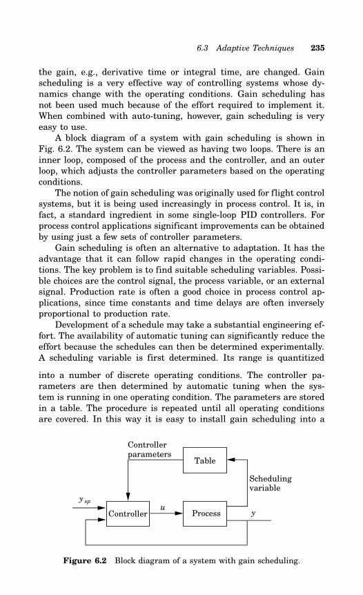
6.3 Adaptive Techniques 235
the gain, e.g., derivative time or integral time, are changed. Gainscheduling is a very effective way of controlling systems whose dy-namics change with the operating conditions. Gain scheduling hasnot been used much because of the effort required to implement it.When combined with auto-tuning, however, gain scheduling is veryeasy to use.A block diagram of a system with gain scheduling is shown in
Fig. 6.2. The system can be viewed as having two loops. There is aninner loop, composed of the process and the controller, and an outerloop, which adjusts the controller parameters based on the operatingconditions.The notion of gain scheduling was originally used for flight control
systems, but it is being used increasingly in process control. It is, infact, a standard ingredient in some single-loop PID controllers. Forprocess control applications significant improvements can be obtainedby using just a few sets of controller parameters.Gain scheduling is often an alternative to adaptation. It has the
advantage that it can follow rapid changes in the operating condi-tions. The key problem is to find suitable scheduling variables. Possi-ble choices are the control signal, the process variable, or an externalsignal. Production rate is often a good choice in process control ap-plications, since time constants and time delays are often inverselyproportional to production rate.Development of a schedule may take a substantial engineering ef-
fort. The availability of automatic tuning can significantly reduce theeffort because the schedules can then be determined experimentally.A scheduling variable is first determined. Its range is quantitized
into a number of discrete operating conditions. The controller pa-rameters are then determined by automatic tuning when the sys-tem is running in one operating condition. The parameters are storedin a table. The procedure is repeated until all operating conditionsare covered. In this way it is easy to install gain scheduling into a
ProcessController
Table
y sp
yu
Controllerparameters
Schedulingvariable
Figure 6.2 Block diagram of a system with gain scheduling.
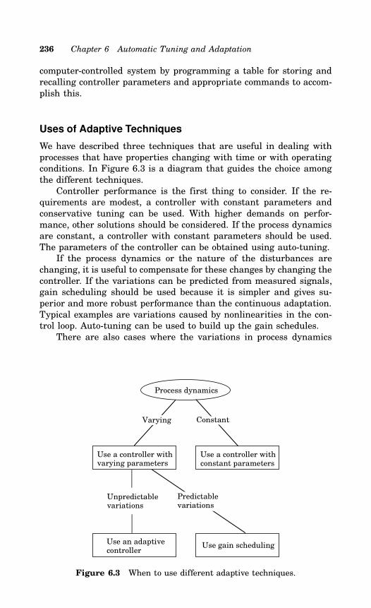
236 Chapter 6 Automatic Tuning and Adaptation
computer-controlled system by programming a table for storing andrecalling controller parameters and appropriate commands to accom-plish this.
Uses of Adaptive Techniques
We have described three techniques that are useful in dealing withprocesses that have properties changing with time or with operatingconditions. In Figure 6.3 is a diagram that guides the choice amongthe different techniques.Controller performance is the first thing to consider. If the re-
quirements are modest, a controller with constant parameters andconservative tuning can be used. With higher demands on perfor-mance, other solutions should be considered. If the process dynamicsare constant, a controller with constant parameters should be used.The parameters of the controller can be obtained using auto-tuning.If the process dynamics or the nature of the disturbances are
changing, it is useful to compensate for these changes by changing thecontroller. If the variations can be predicted from measured signals,gain scheduling should be used because it is simpler and gives su-perior and more robust performance than the continuous adaptation.Typical examples are variations caused by nonlinearities in the con-trol loop. Auto-tuning can be used to build up the gain schedules.There are also cases where the variations in process dynamics
Use a controller withvarying parameters
Unpredictablevariations
Process dynamics
Use a controller withconstant parameters
Use an adaptivecontroller
Use gain scheduling
Varying Constant
Predictable variations
Figure 6.3 When to use different adaptive techniques.
6.4 Model-Based Methods 237
are not predictable. Typical examples are changes due to unmeasur-able variations in raw material, wear, fouling etc. These variationscannot be handled by gain scheduling, since no scheduling variableis available, but must be dealt with by adaptation. An auto-tuningprocedure is often used to initialize the adaptive controller. It is thensometimes called pre-tuning or initial tuning.Feedforward control deserves special mentioning. It is a very pow-
erful method for dealing with measurable disturbances. Use of feed-forward control, however, requires good models of process dynamics.It is difficult to tune feedforward control loops automatically on de-mand, since the operator often cannot manipulate the disturbanceused for the feedforward control. To tune the feedforward controllerit is necessary to wait for an appropriate disturbance. Adaptation,therefore, is particularly useful for the feedforward controller.
6.4 Model-Based Methods
This section gives an overview of automatic tuning approaches thatare based on an explicit derivation of a process model. Models can beobtained in many ways, as seen in Chapter 2. In this section we dis-cuss approaches based on transient responses, frequency responses,and parameter estimation.
Transient Response Methods
Auto-tuners can be based on open-loop or closed-loop transient re-sponse analysis. Methods for determining the transient response werediscussed in Section 2.3. The most common methods are based on stepor pulse responses, but there are also methods that can use manyother types of perturbations.
Open-Loop Tuning
A simple process model can be obtained from an open-loop transientresponse experiment. A step or a pulse is injected at the process input,and the response is measured. To perform such an experiment, theprocess must be stable. If a pulse test is used, the process may includean integrator. It is necessary that the process be in equilibrium whenthe experiment is begun.There are, in principle, only one or two parameters that must
be set a priori, namely the amplitude and the signal duration. Theamplitude should be chosen sufficiently large, so that the responseis easily visible above the noise level. On the other hand, it should
238 Chapter 6 Automatic Tuning and Adaptation
be as small as possible in order not to disturb the process more thannecessary and to keep the dynamics linear. The noise level can bedetermined automatically at the beginning of the tuning experiment.However, even if the noise level is known, we cannot decide a suitablemagnitude of a step in the control signal without knowing the gain ofthe process. Therefore, it must be possible for the operator to decidethe magnitude.The duration of the experiment is the second parameter that
normally is set a priori. If the process is unknown, it is very difficultto determine whether a step response has settled or not. An intuitiveapproach is to say that the measurement signal has reached its newsteady state if its rate of change is sufficiently small. The rate ofchange is related, however, to the time constants of the process, whichare unknown. If a pulse test is used, the duration of the pulse shouldalso be related to the process time constants.Many methods can be used to extract process characteristics from
a transient response experiment. Most auto-tuners determine thestatic gain, the dominant time constant, and the apparent dead time.The static gain is easy to find accurately from a step-response exper-iment by comparing the stationary values of the control signal andthe measurement signal before and after the step change. The timeconstant and the dead time can be obtained in several ways (see Sec-tion 2.3). The method of moments, presented in Section 2.4, is anappealing method, which is relatively insensitive to high-frequencydisturbances.The transient response methods are often used in a pre-tuning
mode in more complicated tuning devices. The main advantage ofthe methods, namely that they require little prior knowledge, is thenexploited. It is also easy to explain the methods to plant personnel.The main drawback with the transient response methods is that theyare sensitive to disturbances. This drawback is less important if theyare used only in the pre-tuning phase.
Closed-Loop Tuning
Automatic tuning based on transient response identification can alsobe performed on line. The steps or pulses are then added either tothe setpoint or to the control signal. There are also auto-tuners thatdo not introduce any transient disturbances. Perturbations caused bysetpoint changes or load disturbances are used instead. In these casesit is necessary to detect that the perturbations are sufficiently largecompared to the noise level.Closed-loop tuning methods cannot be used on unknown pro-
cesses. Some kind of pre-tuning must always be performed in orderto close the loop in a satisfactory way. On the other hand, they do notusually require any additional a priori information. The magnitude of
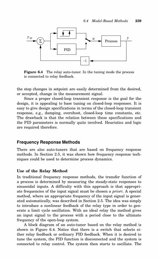
6.4 Model-Based Methods 239
ProcessΣ
−1
PID
yu y sp
Figure 6.4 The relay auto-tuner. In the tuning mode the processis connected to relay feedback.
the step changes in setpoint are easily determined from the desired,or accepted, change in the measurement signal.Since a proper closed-loop transient response is the goal for the
design, it is appealing to base tuning on closed-loop responses. It iseasy to give design specifications in terms of the closed-loop transientresponse, e.g., damping, overshoot, closed-loop time constants, etc.The drawback is that the relation between these specifications andthe PID parameters is normally quite involved. Heuristics and logicare required therefore.
Frequency Response Methods
There are also auto-tuners that are based on frequency responsemethods. In Section 2.5, it was shown how frequency response tech-niques could be used to determine process dynamics.
Use of the Relay Method
In traditional frequency response methods, the transfer function ofa process is determined by measuring the steady-state responses tosinusoidal inputs. A difficulty with this approach is that appropri-ate frequencies of the input signal must be chosen a priori. A specialmethod, where an appropriate frequency of the input signal is gener-ated automatically, was described in Section 2.5. The idea was simplyto introduce a nonlinear feedback of the relay type in order to gen-erate a limit cycle oscillation. With an ideal relay the method givesan input signal to the process with a period close to the ultimatefrequency of the open-loop system.A block diagram of an auto-tuner based on the relay method is
shown in Figure 6.4. Notice that there is a switch that selects ei-ther relay feedback or ordinary PID feedback. When it is desired totune the system, the PID function is disconnected and the system isconnected to relay control. The system then starts to oscillate. The
240 Chapter 6 Automatic Tuning and Adaptation
period and the amplitude of the oscillation is determined when steady-state oscillation is obtained. This gives the ultimate period and theultimate gain. The parameters of a PID controller can then be de-termined from these values, e.g., using the Ziegler-Nichols frequencyresponse method. The PID controller is then automatically switchedin again, and the control is executed with the new PID parameters.This tuning device has one parameter that must be specified in
advance, namely, the initial amplitude of the relay. A feedback loopfrom measurement of the amplitude of the oscillation to the relayamplitude can be used to ensure that the output is within reasonablebounds during the oscillation. It is also useful to introduce hysteresisin the relay. This reduces the effects of measurement noise and alsoincreases the period of the oscillation. With hysteresis there is anadditional parameter. This can be set automatically, however, basedon a determination of the measurement noise level. Notice that thereis no need to know time scales a priori since the ultimate frequencyis determined automatically.In the relay method, an oscillation with suitable frequency is
generated by a static nonlinearity. Even the order of magnitude ofthe time constant of the process can be unknown. Therefore, thismethod is not only suitable as a tuning device; it can also be used inpre-tuning. It is also suitable for determination of sampling periodsin digital controllers.The relay tuning method also can be modified to identify several
points on the Nyquist curve. This can be accomplished by makingseveral experiments with different values of the amplitude and thehysteresis of the relay. A filter with known characteristics can alsobe introduced in the loop to identify other points on the Nyquistcurve. If the static process gain is determined, the KT tuning methodpresented in Chapter 5 can be used.
On-Line Methods
Frequency response analysis can also be used for on-line tuning of PIDcontrollers. The relay feedback technique can be used, as describedin Section 2.5. By introducing bandpass filters, the signal contentat different frequencies can be investigated. From this knowledge, aprocess model given in terms of points on the Nyquist curve can beidentified on line. In this auto-tuner the choice of frequencies in thebandpass filters is crucial. This choice can be simplified by using thetuning procedure described above in a pre-tuning phase.
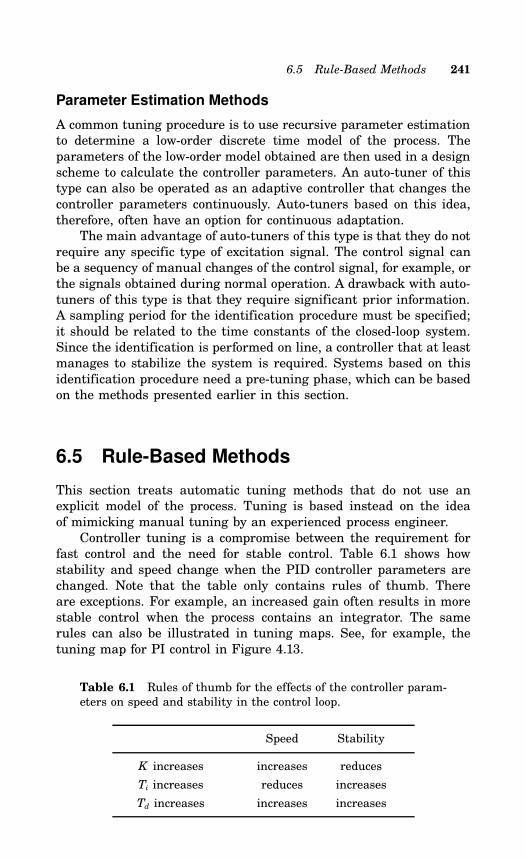
6.5 Rule-Based Methods 241
Parameter Estimation Methods
A common tuning procedure is to use recursive parameter estimationto determine a low-order discrete time model of the process. Theparameters of the low-order model obtained are then used in a designscheme to calculate the controller parameters. An auto-tuner of thistype can also be operated as an adaptive controller that changes thecontroller parameters continuously. Auto-tuners based on this idea,therefore, often have an option for continuous adaptation.The main advantage of auto-tuners of this type is that they do not
require any specific type of excitation signal. The control signal canbe a sequency of manual changes of the control signal, for example, orthe signals obtained during normal operation. A drawback with auto-tuners of this type is that they require significant prior information.A sampling period for the identification procedure must be specified;it should be related to the time constants of the closed-loop system.Since the identification is performed on line, a controller that at leastmanages to stabilize the system is required. Systems based on thisidentification procedure need a pre-tuning phase, which can be basedon the methods presented earlier in this section.
6.5 Rule-Based Methods
This section treats automatic tuning methods that do not use anexplicit model of the process. Tuning is based instead on the ideaof mimicking manual tuning by an experienced process engineer.Controller tuning is a compromise between the requirement for
fast control and the need for stable control. Table 6.1 shows howstability and speed change when the PID controller parameters arechanged. Note that the table only contains rules of thumb. Thereare exceptions. For example, an increased gain often results in morestable control when the process contains an integrator. The samerules can also be illustrated in tuning maps. See, for example, thetuning map for PI control in Figure 4.13.
Table 6.1 Rules of thumb for the effects of the controller param-eters on speed and stability in the control loop.
Speed Stability
K increases increases reduces
Ti increases reduces increases
Td increases increases increases
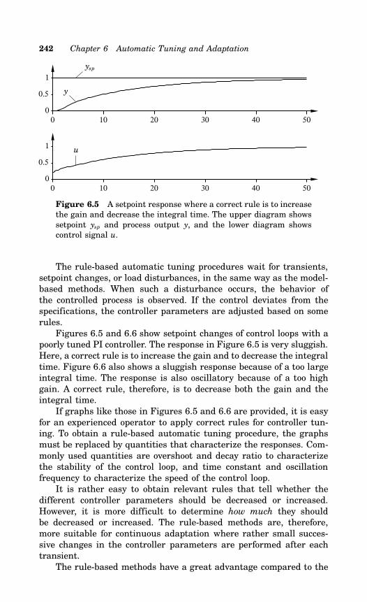
242 Chapter 6 Automatic Tuning and Adaptation
0 10 20 30 40 500
0.5
1
0 10 20 30 40 500
0.5
1
ysp
y
u
Figure 6.5 A setpoint response where a correct rule is to increasethe gain and decrease the integral time. The upper diagram showssetpoint ysp and process output y, and the lower diagram showscontrol signal u.
The rule-based automatic tuning procedures wait for transients,setpoint changes, or load disturbances, in the same way as the model-based methods. When such a disturbance occurs, the behavior ofthe controlled process is observed. If the control deviates from thespecifications, the controller parameters are adjusted based on somerules.Figures 6.5 and 6.6 show setpoint changes of control loops with a
poorly tuned PI controller. The response in Figure 6.5 is very sluggish.Here, a correct rule is to increase the gain and to decrease the integraltime. Figure 6.6 also shows a sluggish response because of a too largeintegral time. The response is also oscillatory because of a too highgain. A correct rule, therefore, is to decrease both the gain and theintegral time.If graphs like those in Figures 6.5 and 6.6 are provided, it is easy
for an experienced operator to apply correct rules for controller tun-ing. To obtain a rule-based automatic tuning procedure, the graphsmust be replaced by quantities that characterize the responses. Com-monly used quantities are overshoot and decay ratio to characterizethe stability of the control loop, and time constant and oscillationfrequency to characterize the speed of the control loop.It is rather easy to obtain relevant rules that tell whether the
different controller parameters should be decreased or increased.However, it is more difficult to determine how much they shouldbe decreased or increased. The rule-based methods are, therefore,more suitable for continuous adaptation where rather small succes-sive changes in the controller parameters are performed after eachtransient.The rule-based methods have a great advantage compared to the
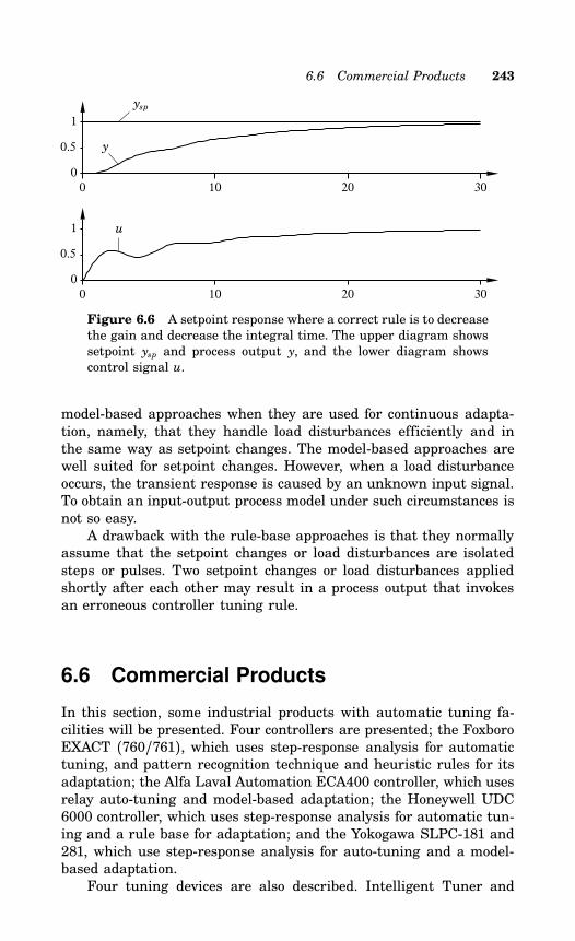
6.6 Commercial Products 243
0 10 20 300
0.5
1
0 10 20 300
0.5
1
ysp
y
u
Figure 6.6 A setpoint response where a correct rule is to decreasethe gain and decrease the integral time. The upper diagram showssetpoint ysp and process output y, and the lower diagram showscontrol signal u.
model-based approaches when they are used for continuous adapta-tion, namely, that they handle load disturbances efficiently and inthe same way as setpoint changes. The model-based approaches arewell suited for setpoint changes. However, when a load disturbanceoccurs, the transient response is caused by an unknown input signal.To obtain an input-output process model under such circumstances isnot so easy.A drawback with the rule-base approaches is that they normally
assume that the setpoint changes or load disturbances are isolatedsteps or pulses. Two setpoint changes or load disturbances appliedshortly after each other may result in a process output that invokesan erroneous controller tuning rule.
6.6 Commercial Products
In this section, some industrial products with automatic tuning fa-cilities will be presented. Four controllers are presented; the FoxboroEXACT (760/761), which uses step-response analysis for automatictuning, and pattern recognition technique and heuristic rules for itsadaptation; the Alfa Laval Automation ECA400 controller, which usesrelay auto-tuning and model-based adaptation; the Honeywell UDC6000 controller, which uses step-response analysis for automatic tun-ing and a rule base for adaptation; and the Yokogawa SLPC-181 and281, which use step-response analysis for auto-tuning and a model-based adaptation.Four tuning devices are also described. Intelligent Tuner and
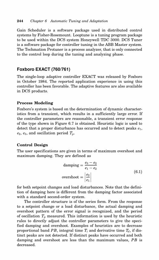
244 Chapter 6 Automatic Tuning and Adaptation
Gain Scheduler is a software package used in distributed controlsystems by Fisher-Rosemount. Looptune is a tuning program packageto be used within the DCS system Honeywell TDC 3000. DCS Tuneris a software package for controller tuning in the ABB Master system.The Techmation Protuner is a process analyzer, that is only connectedto the control loop during the tuning and analyzing phase.
Foxboro EXACT (760/761)
The single-loop adaptive controller EXACT was released by Foxboroin October 1984. The reported application experience in using thiscontroller has been favorable. The adaptive features are also availablein DCS products.
Process Modeling
Foxboro’s system is based on the determination of dynamic character-istics from a transient, which results in a sufficiently large error. Ifthe controller parameters are reasonable, a transient error responseof the type shown in Figure 6.7 is obtained. Heuristic logic is used todetect that a proper disturbance has occurred and to detect peaks e1,e2, e3, and oscillation period Tp.
Control Design
The user specifications are given in terms of maximum overshoot andmaximum damping. They are defined as
damping = e3 − e2e1 − e2
overshoot =∣∣∣∣ e2e1
∣∣∣∣(6.1)
for both setpoint changes and load disturbances. Note that the defini-tion of damping here is different from the damping factor associatedwith a standard second-order system.The controller structure is of the series form. From the response
to a setpoint change or a load disturbance, the actual damping andovershoot pattern of the error signal is recognized, and the periodof oscillation Tp measured. This information is used by the heuristicrules to directly adjust the controller parameters to give the speci-fied damping and overshoot. Examples of heuristics are to decreaseproportional band PB, integral time Ti and derivative time Td, if dis-tinct peaks are not detected. If distinct peaks have occurred and bothdamping and overshoot are less than the maximum values, PB isdecreased.
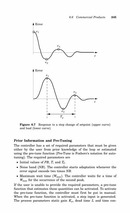
6.6 Commercial Products 245
Error
t
Error
e3
e2
e1
t
Tp
e2
e1
e3
Figure 6.7 Response to a step change of setpoint (upper curve)and load (lower curve).
Prior Information and Pre-Tuning
The controller has a set of required parameters that must be giveneither by the user from prior knowledge of the loop or estimatedusing the pre-tune function (Pre-Tune is Foxboro’s notation for auto-tuning). The required parameters are
• Initial values of PB, Ti and Td.
• Noise band (NB). The controller starts adaptation whenever theerror signal exceeds two times NB.
• Maximum wait time (Wmax). The controller waits for a time ofWmax for the occurrence of the second peak.
If the user is unable to provide the required parameters, a pre-tunefunction that estimates these quantities can be activated. To activatethe pre-tune function, the controller must first be put in manual.When the pre-tune function is activated, a step input is generated.The process parameters static gain Kp, dead time L and time con-
246 Chapter 6 Automatic Tuning and Adaptation
stant T are then obtained from a simple analysis of the process reac-tion curve. The controller parameters are calculated using a Ziegler-Nichols-like formula:
PB = 120KpL/TTi = 1.5LTd = Ti/6
(6.2)
Notice that the controller is parameterized in the series form. Max-imum wait time, Wmax, is also determined from the step responseas:
Wmax = 5L
The noise band is determined during the last phase of the pre-tunemode. The control signal is first returned to the level before the stepchange. With the controller still in manual and the control signal heldconstant, the output is passed through a high-pass filter. The noiseband is calculated as an estimate of the peak-to-peak amplitude ofthe output from the high-pass filter.The estimated noise band (NB) is used to initialize the derivative
term. Derivative action is decreased when the noise level is high inorder to avoid large fluctuations in the control signal. The derivativeterm is initialized using the following logic:
1. Calculate a quantity Z = (3.0− 2NB)/2.5;2. if Z > 1 then set Td = Ti/6;3. if Z < 0 then set Td = 0;4. if 0 < Z < 1 then set Td = Z ⋅ Ti/6.Apart from the set of required parameters, there is also a set ofoptional parameters. If these are not supplied by the user then thedefault values will be used. The optional parameters are as follows(default values in parenthesis):
• Maximum allowed damping (0.3)• Maximum allowed overshoot (0.5)• Derivative factor (1). The derivative term is multiplied by thederivative factor. This allows the derivative influence to be ad-justed by the user. Setting the derivative factor to zero results inPI control.
• Change Limit (10). This factor limits the controller parametersto a certain range. Thus, the controller will not set the PB, Ti andTd values higher than ten times or lower than one tenth of theirinitial values if the default of 10 is used for the change limit.
6.6 Commercial Products 247
Alfa Laval Automation ECA400
This controller was announced by Alfa Laval Automation in 1988. Ithas the adaptive functions of automatic tuning, gain scheduling, andcontinuous adaptation of feedback and feedforward control. An earlierproduct, ECA40, which only has auto-tuning and gain scheduling wasannounced in 1986.
Automatic Tuning
The auto-tuning is performed using the relay method in the followingway. The process is brought to a desired operating point, either bythe operator in manual mode or by a previously tuned controller inautomatic mode. When the loop is stationary, the operator presses atuning button. After a short period, when the noise level is measuredautomatically, a relay with hysteresis is introduced in the loop, andthe PID controller is temporarily disconnected (see Figure 6.4). Thehysteresis of the relay is determined automatically from the noiselevel. During the oscillation, the relay amplitude is adjusted so thata desired level of the oscillation amplitude is obtained. When anoscillation with constant amplitude and period is obtained, the relayexperiment is interrupted and Gp(iω 0), i.e., the value of the transferfunction Gp at oscillation frequency ω 0, is calculated using describingfunction analysis.
Control Design
The PID algorithm in the ECA400 controller is of series form. Theidentification procedure provides a process model in terms of onepoint Gp(iω 0) on the Nyquist curve. By introducing the PID controllerGc(iω ) in the control loop, it is possible to give the Nyquist curve ofthe compensated system GpGc a desired location at frequency ω 0.For most purposes, the PID parameters are chosen so that Gp(iω 0)is moved to the point where
Gp(iω 0)Gc(iω 0) = 0.5e−i135π /180 (6.3)This design method can be viewed as a combination of phase- andamplitude-margin specification. Since there are three adjustable pa-rameters, K , Ti, and Td, and the design criterion (6.3) only specifiestwo parameters, it is required, furthermore, that
Ti = 4Td (6.4)For some simple control problems, where the process is approximatelya first-order system, the derivative action is switched off and only aPI controller is used. This kind of process is automatically detected.
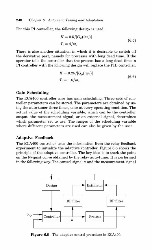
248 Chapter 6 Automatic Tuning and Adaptation
For this PI controller, the following design is used:
K = 0.5/Gp(iω 0)Ti = 4/ω 0
(6.5)
There is also another situation in which it is desirable to switch offthe derivative part, namely for processes with long dead time. If theoperator tells the controller that the process has a long dead time, aPI controller with the following design will replace the PID controller.
K = 0.25/Gp(iω 0)Ti = 1.6/ω 0
(6.6)
Gain Scheduling
The ECA400 controller also has gain scheduling. Three sets of con-troller parameters can be stored. The parameters are obtained by us-ing the auto-tuner three times, once at every operating condition. Theactual value of the scheduling variable, which can be the controlleroutput, the measurement signal, or an external signal, determineswhich parameter set to use. The ranges of the scheduling variablewhere different parameters are used can also be given by the user.
Adaptive Feedback
The ECA400 controller uses the information from the relay feedbackexperiment to initialize the adaptive controller. Figure 6.8 shows theprinciple of the adaptive controller. The key idea is to track the pointon the Nyquist curve obtained by the relay auto-tuner. It is performedin the following way. The control signal u and the measurement signal
y u
y sp
Controller
Design Estimator
BP filter
Process
BP filter
Figure 6.8 The adaptive control procedure in ECA400.
6.6 Commercial Products 249
y are filtered through narrow band-pass filters centered at frequencyω 0. This frequency is obtained from the relay experiment. The signalsare then analyzed in a least-squares estimator which, provides anestimate of the point Gp(iω 0).
Adaptive Feedforward Control
Adaptive feedforward is another feature in ECA400. The adaptivefeedforward control procedure is initialized by the relay auto-tuner.A least-squares algorithm is used to identify parameters a and b inthe model
y(t) = au(t − 4h) + bv(t− 4h) (6.7)where y is the measurement signal, u is the control signal and v is thedisturbance signal that should be fed forward. The sampling intervalh is determined from the relay experiment as h = T0/8, where T0 isthe oscillation period. The feedforward compensator has the simplestructure
∆uf f (t) = kf f (t)∆v(t) (6.8)where the feedforward gain kf f is calculated from the estimated pro-cess parameters
kf f (t) = −0.8 b(t)a(t) (6.9)
Operator Interface
The initial relay amplitude is given a default value suitable for a widerange of process control applications. This parameter is not criticalsince it will be adjusted after the first half period to give an admissibleamplitude of the limit cycle oscillation. The operation of the auto-tuner is then very simple. To use the tuner, the process is simplybrought to an equilibrium by setting a constant control signal inmanual mode. The tuning is activated by pushing the tuning switch.The controller is automatically switched to automatic mode when thetuning is complete.The width of the hysteresis is set automatically, based on mea-
surement of the noise level in the process. The lower the noise level,the lower the amplitude required from the measured signal. The relayamplitude is controlled so that the oscillation is kept at a minimumlevel above the noise level.The following are some optional settings that may be set by the
operator:
Control Design [normal, PI, dead time]. The default design method[normal] can result in either a PI or a PID controller depending onwhether the process is of first order or not. (See the discussion about
250 Chapter 6 Automatic Tuning and Adaptation
control design above.) The operator can force the controller to be PIby selecting [PI]. The PI design method suited for processes with longdead time is chosen by selecting the option [dead time]. The controldesign can be changed either before or after a tuning, as well asduring the adaptation.
Reset [Yes/No]. A reset of information concerning the auto-tuner,the gain-scheduling, or the adaptive controller can be done. Someinformation from a tuning is saved and used to improve the accuracyof the subsequent tunings, including the noise level, the initial relayamplitude, and the period of the oscillation. If a major change ismade in the control loop, for instance if the controller is moved toanother loop, the operator can reset the tuning information. Resettingthe adaptive controller will reset the controller parameters to thoseobtained by the relay auto-tuner.
Initial relay amplitude. In some very sensitive loops, the initialinput step of the relay experiment may be too large. The initial stepcan then be changed by the operator.
Gain scheduling reference. The switches between the differentsets of PID parameters in the gain-scheduling table can be performedwith different choices of the scheduling reference. The scheduling canbe based on the control signal, the measurement signal, or an externalsignal. The gain scheduling is active only when a reference signal isconfigured.
Honeywell UDC 6000
The Honeywell UDC 6000 controller has an adaptive function calledAccutune. Accutune uses both model-based procedures and rule-basedprocedures. It can only be used on stable processes. Consequently,integrating processes can not be treated.
Initial Tuning
The adaptive procedure is initialized by a step-response experiment.The user brings the process variable to a point some distance awayfrom the desired setpoint in manual and waits for steady state.Switching to automatic mode will initiate an open-loop step responseexperiment, where the size of the step is calculated to be so large thatit is supposed to take the process variable to the setpoint.During the experiment, the process variable and its derivative
are continuously monitored. Dead time L is calculated as the timeinterval between the step change and the moment the process variablecrosses a certain small limit.If the derivative of the process variable continuously decreases
from the start, it is concluded that the process is of first order. Static
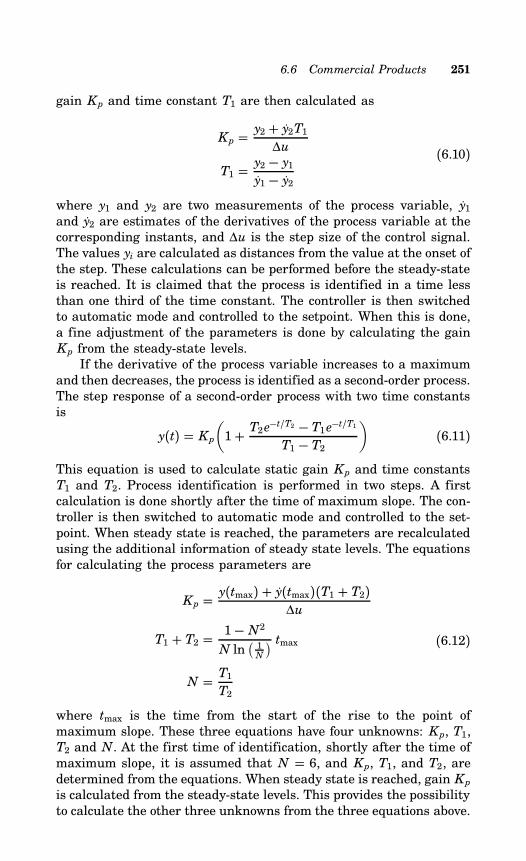
6.6 Commercial Products 251
gain Kp and time constant T1 are then calculated as
Kp = y2 + y2T1∆u
T1 = y2 − y1y1 − y2
(6.10)
where y1 and y2 are two measurements of the process variable, y1and y2 are estimates of the derivatives of the process variable at thecorresponding instants, and ∆u is the step size of the control signal.The values yi are calculated as distances from the value at the onset ofthe step. These calculations can be performed before the steady-stateis reached. It is claimed that the process is identified in a time lessthan one third of the time constant. The controller is then switchedto automatic mode and controlled to the setpoint. When this is done,a fine adjustment of the parameters is done by calculating the gainKp from the steady-state levels.If the derivative of the process variable increases to a maximum
and then decreases, the process is identified as a second-order process.The step response of a second-order process with two time constantsis
y(t) = Kp(1+ T2e
−t/T2 − T1e−t/T1T1 − T2
)(6.11)
This equation is used to calculate static gain Kp and time constantsT1 and T2. Process identification is performed in two steps. A firstcalculation is done shortly after the time of maximum slope. The con-troller is then switched to automatic mode and controlled to the set-point. When steady state is reached, the parameters are recalculatedusing the additional information of steady state levels. The equationsfor calculating the process parameters are
Kp = y(tmax) + y(tmax)(T1 + T2)∆u
T1 + T2 = 1− N2N ln
(1N
) tmaxN = T1
T2
(6.12)
where tmax is the time from the start of the rise to the point ofmaximum slope. These three equations have four unknowns: Kp, T1,T2 and N. At the first time of identification, shortly after the time ofmaximum slope, it is assumed that N = 6, and Kp, T1, and T2, aredetermined from the equations. When steady state is reached, gain Kpis calculated from the steady-state levels. This provides the possibilityto calculate the other three unknowns from the three equations above.
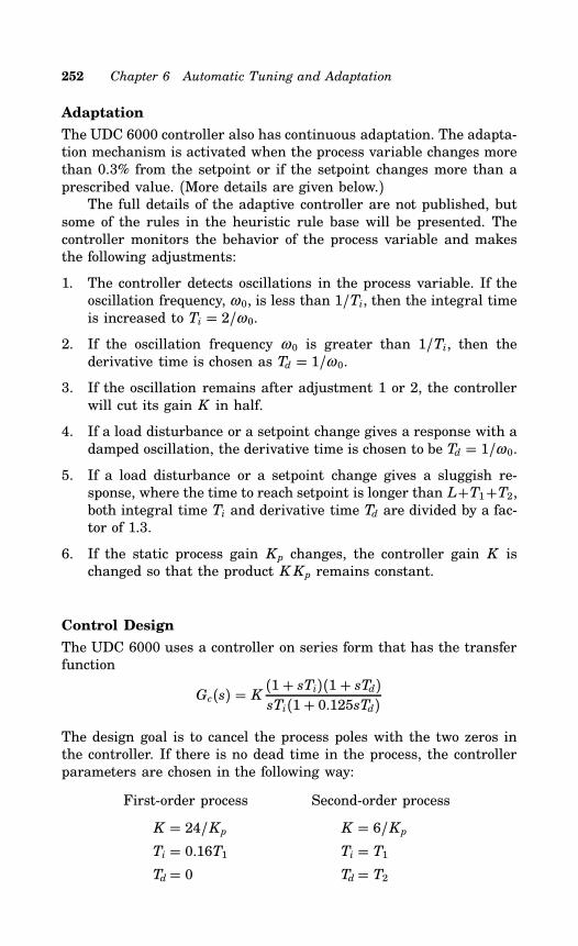
252 Chapter 6 Automatic Tuning and Adaptation
Adaptation
The UDC 6000 controller also has continuous adaptation. The adapta-tion mechanism is activated when the process variable changes morethan 0.3% from the setpoint or if the setpoint changes more than aprescribed value. (More details are given below.)The full details of the adaptive controller are not published, but
some of the rules in the heuristic rule base will be presented. Thecontroller monitors the behavior of the process variable and makesthe following adjustments:
1. The controller detects oscillations in the process variable. If theoscillation frequency, ω 0, is less than 1/Ti, then the integral timeis increased to Ti = 2/ω 0.
2. If the oscillation frequency ω 0 is greater than 1/Ti, then thederivative time is chosen as Td = 1/ω 0.
3. If the oscillation remains after adjustment 1 or 2, the controllerwill cut its gain K in half.
4. If a load disturbance or a setpoint change gives a response with adamped oscillation, the derivative time is chosen to be Td = 1/ω 0.
5. If a load disturbance or a setpoint change gives a sluggish re-sponse, where the time to reach setpoint is longer than L+T1+T2,both integral time Ti and derivative time Td are divided by a fac-tor of 1.3.
6. If the static process gain Kp changes, the controller gain K ischanged so that the product K Kp remains constant.
Control Design
The UDC 6000 uses a controller on series form that has the transferfunction
Gc(s) = K (1+ sTi)(1+ sTd)sTi(1+ 0.125sTd)
The design goal is to cancel the process poles with the two zeros inthe controller. If there is no dead time in the process, the controllerparameters are chosen in the following way:
First-order process Second-order process
K = 24/Kp K = 6/KpTi = 0.16T1 Ti = T1Td= 0 Td= T2
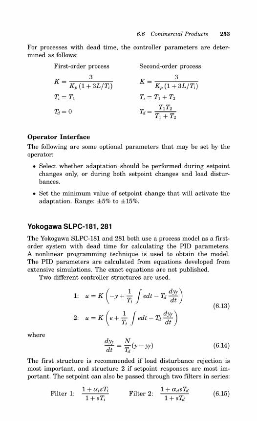
6.6 Commercial Products 253
For processes with dead time, the controller parameters are deter-mined as follows:
First-order process Second-order process
K = 3Kp (1+ 3L/Ti) K = 3
Kp (1+ 3L/Ti)Ti = T1 Ti = T1 + T2Td= 0 Td= T1T2
T1 + T2
Operator Interface
The following are some optional parameters that may be set by theoperator:
• Select whether adaptation should be performed during setpointchanges only, or during both setpoint changes and load distur-bances.
• Set the minimum value of setpoint change that will activate theadaptation. Range: ±5% to ±15%.
Yokogawa SLPC-181, 281
The Yokogawa SLPC-181 and 281 both use a process model as a first-order system with dead time for calculating the PID parameters.A nonlinear programming technique is used to obtain the model.The PID parameters are calculated from equations developed fromextensive simulations. The exact equations are not published.Two different controller structures are used.
1: u = K(−y+ 1
Ti
∫edt− Td dyf
dt
)
2: u = K(e+ 1Ti
∫edt− Td dyf
dt
) (6.13)
wheredyf
dt= NTd(y− yf ) (6.14)
The first structure is recommended if load disturbance rejection ismost important, and structure 2 if setpoint responses are most im-portant. The setpoint can also be passed through two filters in series:
Filter 1:1+α isTi1+ sTi Filter 2:
1+α dsTd1+ sTd (6.15)
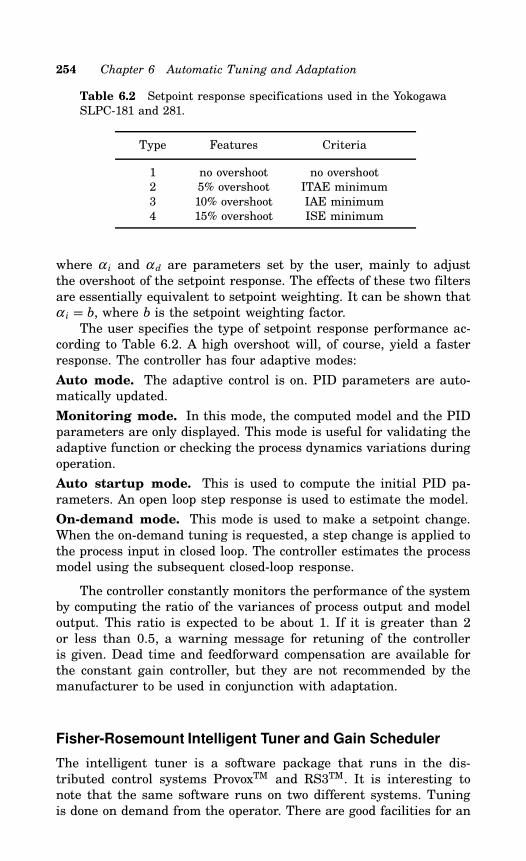
254 Chapter 6 Automatic Tuning and Adaptation
Table 6.2 Setpoint response specifications used in the YokogawaSLPC-181 and 281.
Type Features Criteria
1 no overshoot no overshoot2 5% overshoot ITAE minimum3 10% overshoot IAE minimum4 15% overshoot ISE minimum
where α i and α d are parameters set by the user, mainly to adjustthe overshoot of the setpoint response. The effects of these two filtersare essentially equivalent to setpoint weighting. It can be shown thatα i = b, where b is the setpoint weighting factor.The user specifies the type of setpoint response performance ac-
cording to Table 6.2. A high overshoot will, of course, yield a fasterresponse. The controller has four adaptive modes:
Auto mode. The adaptive control is on. PID parameters are auto-matically updated.
Monitoring mode. In this mode, the computed model and the PIDparameters are only displayed. This mode is useful for validating theadaptive function or checking the process dynamics variations duringoperation.
Auto startup mode. This is used to compute the initial PID pa-rameters. An open loop step response is used to estimate the model.
On-demand mode. This mode is used to make a setpoint change.When the on-demand tuning is requested, a step change is applied tothe process input in closed loop. The controller estimates the processmodel using the subsequent closed-loop response.
The controller constantly monitors the performance of the systemby computing the ratio of the variances of process output and modeloutput. This ratio is expected to be about 1. If it is greater than 2or less than 0.5, a warning message for retuning of the controlleris given. Dead time and feedforward compensation are available forthe constant gain controller, but they are not recommended by themanufacturer to be used in conjunction with adaptation.
Fisher-Rosemount Intelligent Tuner and Gain Scheduler
The intelligent tuner is a software package that runs in the dis-tributed control systems ProvoxTM and RS3TM. It is interesting tonote that the same software runs on two different systems. Tuningis done on demand from the operator. There are good facilities for an
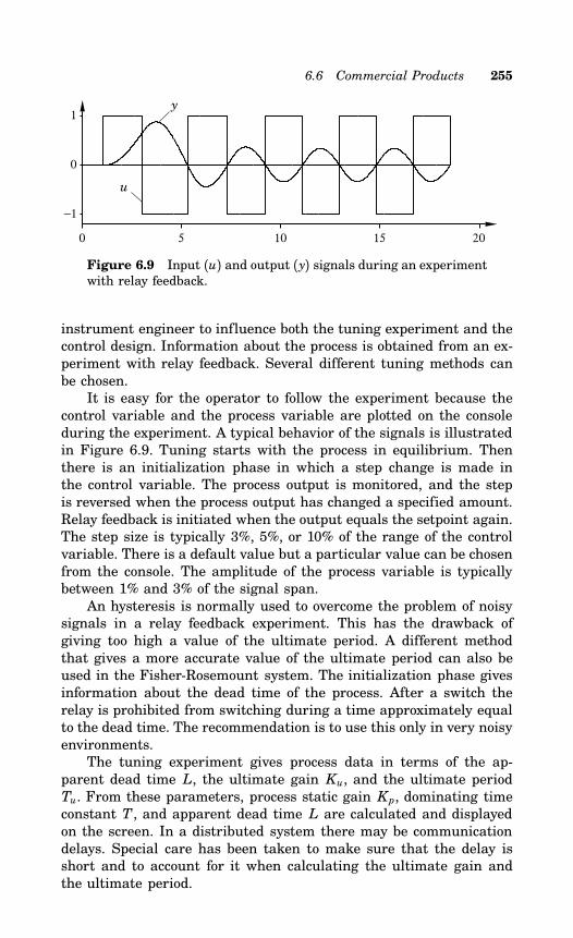
6.6 Commercial Products 255
0 5 10 15 20
−1
0
1y
u
Figure 6.9 Input (u) and output (y) signals during an experimentwith relay feedback.
instrument engineer to influence both the tuning experiment and thecontrol design. Information about the process is obtained from an ex-periment with relay feedback. Several different tuning methods canbe chosen.It is easy for the operator to follow the experiment because the
control variable and the process variable are plotted on the consoleduring the experiment. A typical behavior of the signals is illustratedin Figure 6.9. Tuning starts with the process in equilibrium. Thenthere is an initialization phase in which a step change is made inthe control variable. The process output is monitored, and the stepis reversed when the process output has changed a specified amount.Relay feedback is initiated when the output equals the setpoint again.The step size is typically 3%, 5%, or 10% of the range of the controlvariable. There is a default value but a particular value can be chosenfrom the console. The amplitude of the process variable is typicallybetween 1% and 3% of the signal span.An hysteresis is normally used to overcome the problem of noisy
signals in a relay feedback experiment. This has the drawback ofgiving too high a value of the ultimate period. A different methodthat gives a more accurate value of the ultimate period can also beused in the Fisher-Rosemount system. The initialization phase givesinformation about the dead time of the process. After a switch therelay is prohibited from switching during a time approximately equalto the dead time. The recommendation is to use this only in very noisyenvironments.The tuning experiment gives process data in terms of the ap-
parent dead time L, the ultimate gain Ku, and the ultimate periodTu. From these parameters, process static gain Kp, dominating timeconstant T , and apparent dead time L are calculated and displayedon the screen. In a distributed system there may be communicationdelays. Special care has been taken to make sure that the delay isshort and to account for it when calculating the ultimate gain andthe ultimate period.
256 Chapter 6 Automatic Tuning and Adaptation
Tuning is done from a display that can be brought up on theconsole. The display shows curves; it also has menus and buttonsto execute the tuning. The program has the following methods forcomputing the controller parameters.
PID Standard PID controller with a design that gives a mod-erately fast response with small overshoot and a phasemargin of about 45.
PID-60 PID controller with slow response and small overshoot.
P Proportional controller with Ziegler-Nichols design.
PI PI control based on Ziegler-Nichols design.
PID-ZN PID controller based on Ziegler-Nichols design, fast butwith considerable overshoot.
PID-45N PID control for a noisy control loop. The controller has 45
phase margin and less derivative action than the standardPID design.
PID-60N Similar to PID-45N but with less overshoot.
PI-DT PI design for processes with dominating dead time, smallergain and integral time than the PI design.
IMC Design based on the internal model principle. (See Section4.5.) The details are not available. This design does notwork for processes with integral action.
IMC-NSR Similar to IMC design for processes with integral action.
There are also recommendations for choosing different control de-signs. PI control is the primary choice for flow-pressure and levelcontrol, while PID is recommended for pH and temperature control.In addition, the closed loop can be modified by selecting SLOW, NOR-MAL, or FAST. With these choices the controller gain is multipliedwith the factors 0.50, 1.00, and 1.25. It is possible to change the designwithout retuning the process.After a tuning the new controller parameters are displayed to-
gether with the old controller parameters. It is then possible to accept,reject, redesign, or modify the controller parameters.The intelligent gain scheduler is a complement to the tuner. The
scheduling variable is the process variable, the control variable, or anexternal signal. The range of the scheduling variable is divided intothree regions. The values of the controller parameters in each regionare stored in a table. Interpolation between the entries is done witha fuzzy scheme. Values from the tuner are entered automatically inthe tables. They can also be entered manually.Typical applications of gain scheduling are pH control, split-range
control, level control in vessels with unusual geometries, and surgetank control.
6.6 Commercial Products 257
Honeywell Looptune
Looptune is a tuning-program package for the DCS system HoneywellTDC 3000. It offers the following features:
• A search algorithm, which performs incremental improvementsof the controller parameters until an optimum is reached.
• A relay feedback technique to tune the controller according to theZiegler-Nichols frequency response method.
• Gain scheduling, where the schedule contains three sets of con-troller parameters.
In this presentation, we focus on the search algorithm.
The Objective Function
The control performance is optimized by adjusting the controller pa-rameters in such a way that an objective function (J) is minimized.The objective function is
J = (1−w)σ 2e +wσ 2u
where σ 2e is the variance of the control error e = ysp − y; σ 2u is thevariance of the control signal; and w is a weighting factor with range0 ≤ w ≤ 1, specified by the user. (This is the only parameter thathas to be specified by the user.) If a small value of w is chosen, theerror variance term dominates the objective function. This means thatobjective function J is minimized if the controller is tuned for tightcontrol. If w is large, the control signal variance term dominates, andobjective function J is minimized when the controller is tuned to givea smoother control with smaller control actions.The objective function is calculated in the following way. Setpoint
ysp, process output y, and control signal u are registered during anevaluation period. The variance of the control error (σ 2e ) and thevariance of the control signal (σ 2u) are then calculated in the followingway:
σ 2e =1n
n∑i=1(ysp(i) − y(i))2
σ 2u =1n
n∑i=1(u(i) − u)2
where n is the number of data points and
u = 1n
n∑i=1u(i)
is the mean value of the control signal during the evaluation period.
258 Chapter 6 Automatic Tuning and Adaptation
The Search Procedure
The procedure consists of the following steps:
1. Collect n new values of ysp, y, and u during an evaluation period.
2. Compute the value of the objective function and compare it withthe previous value.
3. If the value of the objective function has decreased, the controllerparameter is adjusted further in the same direction, otherwisethe direction is reversed.
4. If the value of the objective function has reached its minimum,then stop the adjustment. If not, go back to step 1 again.
When a controller parameter has been adjusted according to theserules, the Looptuner goes on to the next controller parameter andstarts to adjust it to an optimal value. It is claimed that normallyseveral passes through the tuning constants are needed in order toarrive at the optimal controller parameters.The evaluation period is a crucial parameter in this tuning pro-
cedure. It is determined automatically and it should be as short aspossible in order to get a fast tuning procedure. On the other hand,it is important that it is long enough, so that a representative num-ber of disturbances occur within the period. At least eight significantdisturbances must occur within the evaluation period. The Looptunealso has a rule-base that compensates the objective functions for vari-ations in the disturbance behavior between the different evaluationperiods.The search procedure in the Looptune has two modes of operation:
One-shot tuning. The tuning is deactivated when all controllerparameters have reached their optimal values.
Continuous adaptation. The adjustments goes on until it is inter-rupted by the operator.
ABB DCS Tuner
This DCS Tuner is a software package for on-line and off-line auto-matic tuning of PID controllers in the ABB Master system. It runs onpersonal computers and is connected to the ABB Master by a seriallink interface. The DCS Tuner has four main functions: process iden-tification, controller tuning, process analysis, and simulation. Thesefour functions are described below.
Process Identification
The process identification can be based on either historical data oron-line data. The on-line data acquisition can be event initiated. This
6.6 Commercial Products 259
means that the data used for process identification can be controlledbased on a high- or low-level triggering. The triggering signal canbe the control error, the process variable, or any other signal loggedduring the session. The major steps performed during the processmodel identification are:
1. Signal filering using Butterworth filters
2. Process dead-time estimation
3. Process model order identification
4. Least-squares identification of continuous-time and discrete-timemodels
5. Process model validation
These steps are normally performed automatically, but the operatormay interfere by changing parameters.
Controller Tuning
The tuning procedure uses the discrete-time model to obtain thecontroller parameters. The tuning method is based on a dominantpole design procedure. The user may select among three differentclosed-loop performances: Fast, Normal, or Damped.
Process Analysis
Three functions are available for process analysis. They are calledStatistics, FFT, and Correlation. The Statistics function provides sta-tistical information about the different data series, such as mean,standard deviation etc. Frequency spectra of the different signalsand frequency domain models of the process can be obtained usingthe Fast Fourier Transform (FFT). Finally, the Correlation functiongives results of auto- and cross-correlation analysis.
Simulation
In the simulation mode, both open-loop and closed-loop simulationare available. The user has access to both controller and process pa-rameters. This provides a possibility to check how different controllersettings suit a certain process model, and also how changes in theprocess model influence the control loop performance.
Techmation Protuner
The Protuner is a process analyzer from Techmation Inc. It consistsof a software package for personal computers and an interface mod-ule with cables to be connected to the process output and the control
260 Chapter 6 Automatic Tuning and Adaptation
signal of the control loop to be analyzed. The Protuner monitors astep-response experiment, calculates the frequency response of theprocess based on the experimental data, and suggests controller pa-rameters based on several methods for controller tuning.
Prior Information
Before the process analysis is performed, the user must provide someinformation about the process and the controller. This is done usinga couple of “Set-up menus.” The following process information mustbe given:
• The ranges of the control and the measurement signals.
• It must be determined if the process is stable or if it has integralaction.
To be able to set relevant controller parameters, the following dataabout the controller must be provided:
• P-type (gain or proportional band)• I-type (seconds, seconds/repeat, minutes, or minutes/repeat)• Controller structure (ideal, series, or parallel)• Sampling rate
• Filter time constant (if there is a low-pass filter connected to themeasurement signal).
Before the tuning experiment can be performed, the user must alsospecify a sample time. This is the time during which data will becollected during the experiment. It is important to choose the sampletime long enough, so that the step response settles before the sampletime has ended. In case of an open-loop experiment of an integratingprocess, the response must reach a constant rate of change when theexperiment ends.
Determining the Process Model
The tuning procedure is based on a step-response experiment. It canbe performed either in open or closed loop. The open-loop experimentis recommended. When the user gives a start command, the processoutput and the control signal are displayed on the screen, with a timeaxis that is given by the sample time defined by the user. The userthen makes a step change in the control signal. If the experiment isperformed in closed loop a step is instead introduced in the setpoint.There are several facilities for editing the data obtained from the
step-response experiment. Outliers can be removed and data can befiltered. These features are very useful because they make it possi-ble to overcome problems that are often encountered when makingexperiments on industrial processes.
6.6 Commercial Products 261
When the data has been edited the Protuner calculates the fre-quency response of the process. The result can be displayed in a Bodediagram, a Nyquist diagram, or a Nichols diagram. The static gain,the dominant time constant and the apparent dead time are also dis-played, as well as the ultimate gain and the ultimate period.
Design Calculations
The controller parameters are calculated from the frequency response.A special technique is used. This is based on cancellation of processpoles by controller zeros. The integral time and the derivative timeare first determined to perform this cancellation. The gain is thendetermined to meet predetermined gain and phase margins.The Protuner provides several design options. Controller param-
eters are given for the following closed-loop responses:
Slow: Critically damped response.
Medium: Slightly underdamped response.
Fast: Response with decay ratio 0.38.
The different design options are obtained by specifying different val-ues of the gain and the phase margins. The Protuner provides differ-ent controller parameters depending on whether setpoint or load dis-turbances are considered. Both P, PI, and PID controller parametersare provided. The setpoint weightings for proportional and derivativeaction and the high frequency gain at the derivative part must besupplied by the user.
Evaluation
It is possible to evaluate the performance of the closed-loop systemin several ways. The combined frequency response, i.e., the frequencyresponse of the loop transfer function
G(iω ) = Gp(iω )Gc(iω )
where Gp(iω ) is the process transfer function and Gc(iω ) is the con-troller transfer function, can be plotted in a Bode diagram, a Nyquistdiagram, or a Nichols diagram. In this way, the phase and amplitudemargins or the Ms value can be checked.The Protuner also has a simulation facility. It is possible to sim-
ulate the closed-loop response of the process and the suggested con-troller. To do this, it is necessary to provide some additional controllerparameters, namely setpoint weightings b and c, and derivative gainlimitation factor N. Using the simulation facility, it is also possibleto investigate the effects of noise and to design filters to reduce theseeffects.
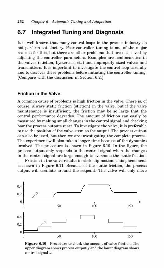
262 Chapter 6 Automatic Tuning and Adaptation
6.7 Integrated Tuning and Diagnosis
It is well known that many control loops in the process industry donot perform satisfactory. Poor controller tuning is one of the majorreasons for this, but there are other problems that are not solved byadjusting the controller parameters. Examples are nonlinearities inthe valves (stiction, hysteresis, etc) and improperly sized valves andtransmitters. It is important to investigate the control loop carefullyand to discover these problems before initiating the controller tuning.(Compare with the discussion in Section 6.2.)
Friction in the Valve
A common cause of problems is high friction in the valve. There is, ofcourse, always static friction (stiction) in the valve, but if the valvemaintenance is insufficient, the friction may be so large that thecontrol performance degrades. The amount of friction can easily bemeasured by making small changes in the control signal and checkinghow the process outputs react. To investigate the valve, it is preferableto use the position of the valve stem as the output. The process outputcan also be used, but then we are investigating the complete process.The experiment will also take a longer time because of the dynamicsinvolved. The procedure is shown in Figure 6.10. In the figure, theprocess output only responds to the control signal when the changesin the control signal are large enough to overcome the static friction.Friction in the valve results in stick-slip motion. This phenomena
is shown in Figure 6.11. Because of the static friction, the processoutput will oscillate around the setpoint. The valve will only move
0 50 100 1500
0.2
0.4
0 50 100 1500
0.2
0.4
y
u
Figure 6.10 Procedure to check the amount of valve friction. Theupper diagram shows process output y and the lower diagram showscontrol signal u.
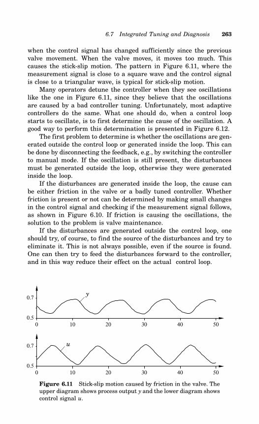
6.7 Integrated Tuning and Diagnosis 263
when the control signal has changed sufficiently since the previousvalve movement. When the valve moves, it moves too much. Thiscauses the stick-slip motion. The pattern in Figure 6.11, where themeasurement signal is close to a square wave and the control signalis close to a triangular wave, is typical for stick-slip motion.Many operators detune the controller when they see oscillations
like the one in Figure 6.11, since they believe that the oscillationsare caused by a bad controller tuning. Unfortunately, most adaptivecontrollers do the same. What one should do, when a control loopstarts to oscillate, is to first determine the cause of the oscillation. Agood way to perform this determination is presented in Figure 6.12.The first problem to determine is whether the oscillations are gen-
erated outside the control loop or generated inside the loop. This canbe done by disconnecting the feedback, e.g., by switching the controllerto manual mode. If the oscillation is still present, the disturbancesmust be generated outside the loop, otherwise they were generatedinside the loop.If the disturbances are generated inside the loop, the cause can
be either friction in the valve or a badly tuned controller. Whetherfriction is present or not can be determined by making small changesin the control signal and checking if the measurement signal follows,as shown in Figure 6.10. If friction is causing the oscillations, thesolution to the problem is valve maintenance.If the disturbances are generated outside the control loop, one
should try, of course, to find the source of the disturbances and try toeliminate it. This is not always possible, even if the source is found.One can then try to feed the disturbances forward to the controller,and in this way reduce their effect on the actual control loop.
0 10 20 30 40 500.5
0.7
0 10 20 30 40 500.5
0.7
y
u
Figure 6.11 Stick-slip motion caused by friction in the valve. Theupper diagram shows process output y and the lower diagram showscontrol signal u.
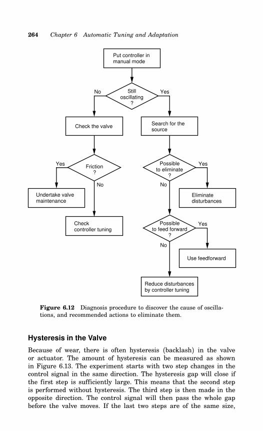
264 Chapter 6 Automatic Tuning and Adaptation
Put controller in manual mode
Possible to feed forward
?
Friction?
Possibleto eliminate
?
Check the valveSearch for the source
Undertake valve maintenance
Eliminate disturbances
Use feedforward
Reduce disturbancesby controller tuning
Check controller tuning
Stilloscillating
?
No Yes
Yes Yes
No No
No
Yes
Figure 6.12 Diagnosis procedure to discover the cause of oscilla-tions, and recommended actions to eliminate them.
Hysteresis in the Valve
Because of wear, there is often hysteresis (backlash) in the valveor actuator. The amount of hysteresis can be measured as shownin Figure 6.13. The experiment starts with two step changes in thecontrol signal in the same direction. The hysteresis gap will close ifthe first step is sufficiently large. This means that the second stepis performed without hysteresis. The third step is then made in theopposite direction. The control signal will then pass the whole gapbefore the valve moves. If the last two steps are of the same size,
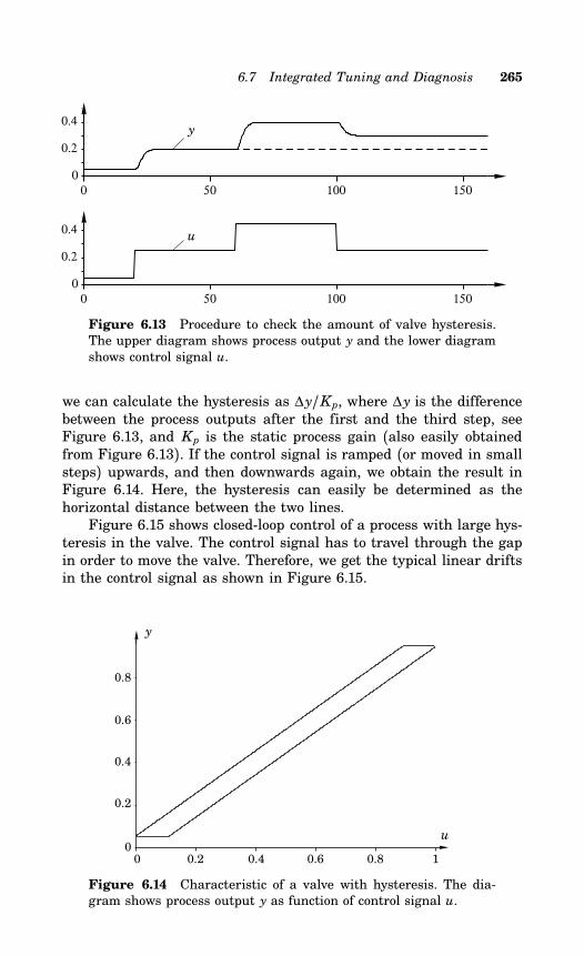
6.7 Integrated Tuning and Diagnosis 265
0 50 100 1500
0.2
0.4
0 50 100 1500
0.2
0.4
y
u
Figure 6.13 Procedure to check the amount of valve hysteresis.The upper diagram shows process output y and the lower diagramshows control signal u.
we can calculate the hysteresis as ∆y/Kp, where ∆y is the differencebetween the process outputs after the first and the third step, seeFigure 6.13, and Kp is the static process gain (also easily obtainedfrom Figure 6.13). If the control signal is ramped (or moved in smallsteps) upwards, and then downwards again, we obtain the result inFigure 6.14. Here, the hysteresis can easily be determined as thehorizontal distance between the two lines.Figure 6.15 shows closed-loop control of a process with large hys-
teresis in the valve. The control signal has to travel through the gapin order to move the valve. Therefore, we get the typical linear driftsin the control signal as shown in Figure 6.15.
u
y
0 0.2 0.4 0.6 0.8 10
0.2
0.4
0.6
0.8
Figure 6.14 Characteristic of a valve with hysteresis. The dia-gram shows process output y as function of control signal u.
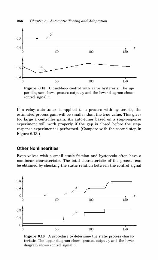
266 Chapter 6 Automatic Tuning and Adaptation
0 50 100 1500.4
0.5
0 50 100 1500.4
0.5
y
u
Figure 6.15 Closed-loop control with valve hysteresis. The up-per diagram shows process output y and the lower diagram showscontrol signal u.
If a relay auto-tuner is applied to a process with hysteresis, theestimated process gain will be smaller than the true value. This givestoo large a controller gain. An auto-tuner based on a step-responseexperiment will work properly if the gap is closed before the step-response experiment is performed. (Compare with the second step inFigure 6.13.)
Other Nonlinearities
Even valves with a small static friction and hysteresis often have anonlinear characteristic. The total characteristic of the process canbe obtained by checking the static relation between the control signal
0 50 100 1500
0.4
0.8
0 50 100 1500
0.4
0.8
y
u
Figure 6.16 A procedure to determine the static process charac-teristic. The upper diagram shows process output y and the lowerdiagram shows control signal u.
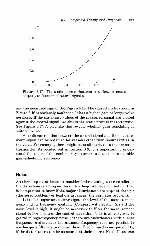
6.7 Integrated Tuning and Diagnosis 267
u
y
0 0.2 0.4 0.6 0.8 10
0.2
0.4
0.6
0.8
Figure 6.17 The static process characteristic, showing processoutput y as function of control signal u.
and the measured signal. See Figure 6.16. The characteristic shown inFigure 6.16 is obviously nonlinear. It has a higher gain at larger valvepositions. If the stationary values of the measured signal are plottedagainst the control signal, we obtain the static process characteristic.See Figure 6.17. A plot like this reveals whether gain scheduling issuitable or not.A nonlinear relation between the control signal and the measure-
ment signal can be obtained for reasons other than nonlinearities inthe valve. For example, there might be nonlinearities in the sensor ortransmitter. As pointed out in Section 6.3, it is important to under-stand the cause of the nonlinearity in order to determine a suitablegain-scheduling reference.
Noise
Another important issue to consider before tuning the controller isthe disturbances acting on the control loop. We have pointed out thatit is important to know if the major disturbances are setpoint changes(the servo problem) or load disturbances (the regulator problem).It is also important to investigate the level of the measurement
noise and its frequency content. (Compare with Section 2.8.) If thenoise level is high, it might be necessary to filter the measurementsignal before it enters the control algorithm. This is an easy way toget rid of high-frequency noise. If there are disturbances with a largefrequency content near the ultimate frequency, it is not possible touse low-pass filtering to remove them. Feedforward is one possibility,if the disturbances can be measured at their source. Notch filters can
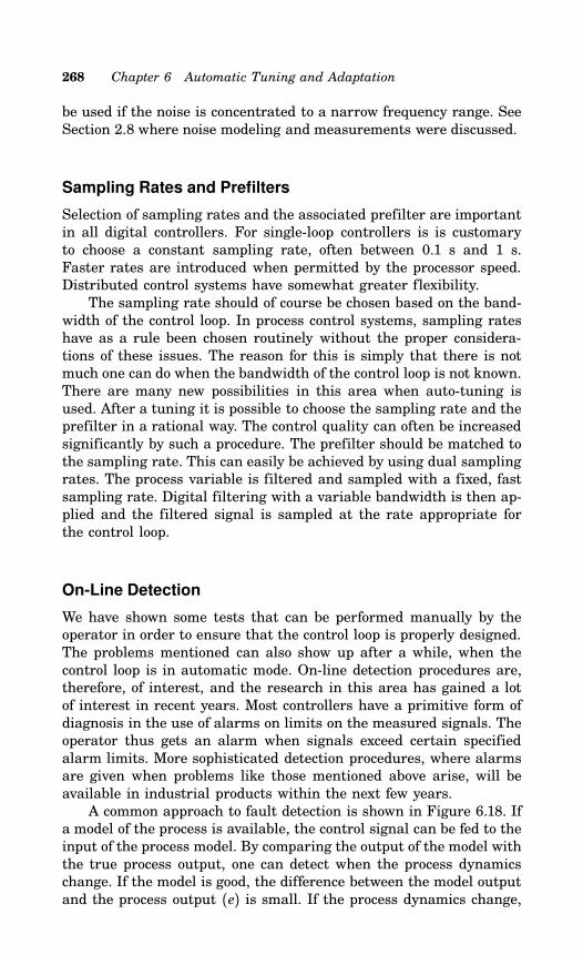
268 Chapter 6 Automatic Tuning and Adaptation
be used if the noise is concentrated to a narrow frequency range. SeeSection 2.8 where noise modeling and measurements were discussed.
Sampling Rates and Prefilters
Selection of sampling rates and the associated prefilter are importantin all digital controllers. For single-loop controllers is is customaryto choose a constant sampling rate, often between 0.1 s and 1 s.Faster rates are introduced when permitted by the processor speed.Distributed control systems have somewhat greater flexibility.The sampling rate should of course be chosen based on the band-
width of the control loop. In process control systems, sampling rateshave as a rule been chosen routinely without the proper considera-tions of these issues. The reason for this is simply that there is notmuch one can do when the bandwidth of the control loop is not known.There are many new possibilities in this area when auto-tuning isused. After a tuning it is possible to choose the sampling rate and theprefilter in a rational way. The control quality can often be increasedsignificantly by such a procedure. The prefilter should be matched tothe sampling rate. This can easily be achieved by using dual samplingrates. The process variable is filtered and sampled with a fixed, fastsampling rate. Digital filtering with a variable bandwidth is then ap-plied and the filtered signal is sampled at the rate appropriate forthe control loop.
On-Line Detection
We have shown some tests that can be performed manually by theoperator in order to ensure that the control loop is properly designed.The problems mentioned can also show up after a while, when thecontrol loop is in automatic mode. On-line detection procedures are,therefore, of interest, and the research in this area has gained a lotof interest in recent years. Most controllers have a primitive form ofdiagnosis in the use of alarms on limits on the measured signals. Theoperator thus gets an alarm when signals exceed certain specifiedalarm limits. More sophisticated detection procedures, where alarmsare given when problems like those mentioned above arise, will beavailable in industrial products within the next few years.A common approach to fault detection is shown in Figure 6.18. If
a model of the process is available, the control signal can be fed to theinput of the process model. By comparing the output of the model withthe true process output, one can detect when the process dynamicschange. If the model is good, the difference between the model outputand the process output (e) is small. If the process dynamics change,
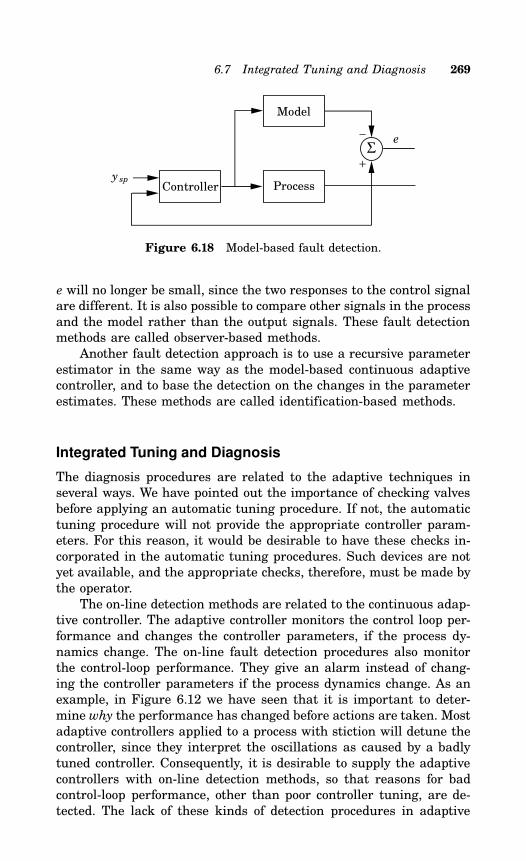
6.7 Integrated Tuning and Diagnosis 269
Σ
Model
e
ProcessController y sp
+
−
Figure 6.18 Model-based fault detection.
e will no longer be small, since the two responses to the control signalare different. It is also possible to compare other signals in the processand the model rather than the output signals. These fault detectionmethods are called observer-based methods.Another fault detection approach is to use a recursive parameter
estimator in the same way as the model-based continuous adaptivecontroller, and to base the detection on the changes in the parameterestimates. These methods are called identification-based methods.
Integrated Tuning and Diagnosis
The diagnosis procedures are related to the adaptive techniques inseveral ways. We have pointed out the importance of checking valvesbefore applying an automatic tuning procedure. If not, the automatictuning procedure will not provide the appropriate controller param-eters. For this reason, it would be desirable to have these checks in-corporated in the automatic tuning procedures. Such devices are notyet available, and the appropriate checks, therefore, must be made bythe operator.The on-line detection methods are related to the continuous adap-
tive controller. The adaptive controller monitors the control loop per-formance and changes the controller parameters, if the process dy-namics change. The on-line fault detection procedures also monitorthe control-loop performance. They give an alarm instead of chang-ing the controller parameters if the process dynamics change. As anexample, in Figure 6.12 we have seen that it is important to deter-mine why the performance has changed before actions are taken. Mostadaptive controllers applied to a process with stiction will detune thecontroller, since they interpret the oscillations as caused by a badlytuned controller. Consequently, it is desirable to supply the adaptivecontrollers with on-line detection methods, so that reasons for badcontrol-loop performance, other than poor controller tuning, are de-tected. The lack of these kinds of detection procedures in adaptive
270 Chapter 6 Automatic Tuning and Adaptation
controllers are perhaps the major reason for the relatively few appli-cations of continuous adaptive control available today.
6.8 Conclusions
The adaptive techniques are relatively new. Even though they havebeen tried industrially for only a few years, there are currently sev-eral thousand loops where adaptive techniques are used. This is nota negligible number, but it is still a very small fraction of all con-trol loops in operation. It is clear that auto-tuning is useful. It cancertainly help operators and instrument engineers keep the controlloops well tuned. The benefits are even larger for more complex loops.For example, the derivative action is often switched off in manuallytuned systems because of tuning problems, in spite of the fact that itimproves performance.Concerning the particular method to use, it is too early to draw
definite conclusions. There are many different ways to determine pro-cess characteristics, many methods for design of PID controllers, andmany ways of combining such techniques to create auto-tuners. Judg-ing from the systems that are now on the market, it appears thatmany different ideas have been successfully implemented. However,some patterns do emerge. It appears that more sophisticated meth-ods require more prior information. This is probably what has led tothe introduction of the pre-tune mode, which often has been an af-terthought. It would seem that a useful approach to this problem isto combine several different approaches. It also seems very naturalto combine adaptive techniques with diagnosis and loop assessment.
6.9 References
Controllers with automatic tuning grew out of research on automaticcontrol. Overviews of adaptive techniques are found in (Dumont,1986), (Åström, 1987a), and (Bristol, 1970). More detailed treat-ments are found in the books (Harris and Billings, 1981), (Åströmand Wittenmark, 1989), and (Hang et al., 1993b). Overviews of dif-ferent approaches and different products are found in (Isermann,1982), (Gawthrop, 1986), (Kaya and Titus, 1988), (Morris, 1987), (Ya-mamoto, 1991), and (Åström et al., 1993).Many different approaches are used in the automatic tuners. The
systems described in (Nishikawa et al., 1984), (Kraus and Myron,1984), and (Takatsu et al., 1991) are based on transient response tech-niques. The paper (Hang and Sin, 1991) is based on cross correlation.
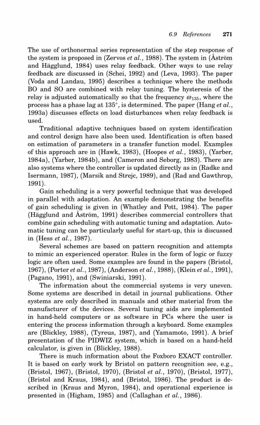
6.9 References 271
The use of orthonormal series representation of the step response ofthe system is proposed in (Zervos et al., 1988). The system in (Åströmand Hägglund, 1984) uses relay feedback. Other ways to use relayfeedback are discussed in (Schei, 1992) and (Leva, 1993). The paper(Voda and Landau, 1995) describes a technique where the methodsBO and SO are combined with relay tuning. The hysteresis of therelay is adjusted automatically so that the frequency ω 135, where theprocess has a phase lag at 135, is determined. The paper (Hang et al.,1993a) discusses effects on load disturbances when relay feedback isused.Traditional adaptive techniques based on system identification
and control design have also been used. Identification is often basedon estimation of parameters in a transfer function model. Examplesof this approach are in (Hawk, 1983), (Hoopes et al., 1983), (Yarber,1984a), (Yarber, 1984b), and (Cameron and Seborg, 1983). There arealso systems where the controller is updated directly as in (Radke andIsermann, 1987), (Marsik and Strejc, 1989), and (Rad and Gawthrop,1991).Gain scheduling is a very powerful technique that was developed
in parallel with adaptation. An example demonstrating the benefitsof gain scheduling is given in (Whatley and Pott, 1984). The paper(Hägglund and Åström, 1991) describes commercial controllers thatcombine gain scheduling with automatic tuning and adaptation. Auto-matic tuning can be particularly useful for start-up, this is discussedin (Hess et al., 1987).Several schemes are based on pattern recognition and attempts
to mimic an experienced operator. Rules in the form of logic or fuzzylogic are often used. Some examples are found in the papers (Bristol,1967), (Porter et al., 1987), (Anderson et al., 1988), (Klein et al., 1991),(Pagano, 1991), and (Swiniarski, 1991).The information about the commercial systems is very uneven.
Some systems are described in detail in journal publications. Othersystems are only described in manuals and other material from themanufacturer of the devices. Several tuning aids are implementedin hand-held computers or as software in PCs where the user isentering the process information through a keyboard. Some examplesare (Blickley, 1988), (Tyreus, 1987), and (Yamamoto, 1991). A briefpresentation of the PIDWIZ system, which is based on a hand-heldcalculator, is given in (Blickley, 1988).There is much information about the Foxboro EXACT controller.
It is based on early work by Bristol on pattern recognition see, e.g.,(Bristol, 1967), (Bristol, 1970), (Bristol et al., 1970), (Bristol, 1977),(Bristol and Kraus, 1984), and (Bristol, 1986). The product is de-scribed in (Kraus and Myron, 1984), and operational experience ispresented in (Higham, 1985) and (Callaghan et al., 1986).
272 Chapter 6 Automatic Tuning and Adaptation
The systems based on relay feedback are also well documented.The principles are presented in (Åström and Hägglund, 1984). Manydetails about implementation and applications are given in (Åströmand Hägglund, 1988) and (Hägglund and Åström, 1991). The con-trollers of this type now include automatic tuning, gain scheduling,and continuous adaptation of feedback and feedforward gains.The papers (McMillan et al., 1993b) and (McMillan et al., 1993a)
describe the Fisher Rosemount products for tuning and gain schedul-ing. The Yokogawa systems are discussed in (Takatsu et al., 1991)and (Yamamoto, 1991).We have not found any journal articles describing the Protuner
and Honeywell’s tuners. The interested reader is recommended tocontact the companies directly.There have been comparisons of different auto-tuners and adap-
tive controllers, but few results from those studies have reached thepublic domain. Some papers that deal with the issue are (Nachtigal,1986a), (Nachtigal, 1986b), (Dumont, 1986), (Dumont et al., 1989).Fault detection and isolation is discussed in (Frank, 1990), (Is-
ermann, 1984), (Isermann et al., 1990), and (Patton et al., 1989).The paper (Hägglund, 1993) describes a fault detection techniquethat has been incorporated in a commercial controller. More elabo-rate controllers that combine control and diagnosis are discussed in(Antsaklis et al., 1991) and (Åström, 1992).
Control Paradigms
7.1 Introduction
So far we have only discussed simple control problems with one controlvariable and one measured signal. Typical process control systemscan be much more complex with many control variables and manymeasured signals. The bottom-up approach is one way to design suchsystems. In this procedure the system is built up from simple com-ponents. The systems can be implemented in many different ways.Originally it was done by interconnection of separate boxes built ofpneumatic or electronic components. Today the systems are typicallyimplemented in distributed control systems consisting of several hi-erarchically connected computers. The software for the distributedcontrol system is typically constructed so that programming can bedone by selecting and interconnecting the components. The key com-ponent, the PID controller, has already been discussed in detail. InSection 3.5 we showed that integrator windup could be avoided byintroducing nonlinearities in the PID controller. In Chapter 6 it wasdemonstrated that controllers could be tuned automatically, also thatthe changes in system behavior could be dealt with by gain schedulingand adaptation. In this chapter, we present some of the other compo-nents required to build complex automation systems. We also presentsome of the key paradigms that guide the construction of complexsystems.A collection of paradigms for control are used to build complex
systems from simple components. The components are controllers ofthe PID type, linear filters, and static nonlinearities. Typical nonlin-earities are amplitude and rate limiters and signal selectors. Feed-back is an important paradigm. Simple feedback loops are used tokeep process variables constant or to make them change in speci-fied ways. (Feedback has been discussed extensively in the previouschapters.) The key problem is to determine the control variables thatshould be chosen to control given process variables. Another problemis that there may be interaction between different feedback loops. Inthis chapter we discuss other paradigms for control. Cascade control
273
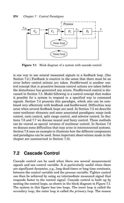
274 Chapter 7 Control Paradigms
Process
Inner loop
y u P1
P2
y sp
y s
Outer loop
CsCp
Figure 7.1 Block diagram of a system with cascade control.
is one way to use several measured signals in a feedback loop. (SeeSection 7.2.) Feedback is reactive in the sense that there must be anerror before control actions are taken. Feedforward is another con-trol concept that is proactive because control actions are taken beforethe disturbance has generated any errors. Feedforward control is dis-cussed in Section 7.3. Model following is a control concept that makesit possible for a system to respond in a specified way to commandsignals. Section 7.4 presents this paradigm, which also can be com-bined very effectively with feedback and feedforward. Difficulties mayarise when several feedback loops are used. In Section 7.5 we describesome nonlinear elements and some associated paradigms: surge tankcontrol, ratio control, split range control, and selector control. In Sec-tions 7.6 and 7.7 we discuss neural and fuzzy control. These methodscan be viewed as special versions of nonlinear control. In Section 7.8we discuss some difficulties that may arize in interconnected systems.Section 7.9 uses an example to illustrate how the different componentsand paradigms can be used. Some important observations made in thechapter are summarized in Section 7.10.
7.2 Cascade Control
Cascade control can be used when there are several measurementsignals and one control variable. It is particularly useful when thereare significant dynamics, e.g., long dead times or long time constants,between the control variable and the process variable. Tighter controlcan then be achieved by using an intermediate measured signal thatresponds faster to the control signal. Cascade control is built up bynesting the control loops, as shown in the block diagram in Figure 7.1.The system in this figure has two loops. The inner loop is called thesecondary loop; the outer loop is called the primary loop. The reason
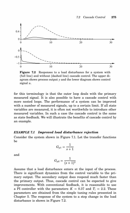
7.2 Cascade Control 275
0 10 20 300
0.4
0 10 20 30−1
−0.5
0
Figure 7.2 Responses to a load disturbance for a system with(full line) and without (dashed line) cascade control. The upper di-agram shows process output y and the lower diagram shows controlsignal u.
for this terminology is that the outer loop deals with the primarymeasured signal. It is also possible to have a cascade control withmore nested loops. The performance of a system can be improvedwith a number of measured signals, up to a certain limit. If all statevariables are measured, it is often not worthwhile to introduce othermeasured variables. In such a case the cascade control is the sameas state feedback. We will illustrate the benefits of cascade control byan example.
EXAMPLE 7.1 Improved load disturbance rejection
Consider the system shown in Figure 7.1. Let the transfer functionsbe
Gp1 = 1s+ 1
and
Gp2 = 1(s+ 1)3
Assume that a load disturbance enters at the input of the process.There is significant dynamics from the control variable to the pri-mary output. The secondary output does respond much faster thanthe primary output. Thus, cascade control can be expected to giveimprovements. With conventional feedback, it is reasonable to usea PI controller with the parameters K = 0.37 and Ti = 2.2. Theseparameters are obtained from the simple tuning rules presented inChapter 5. The response of the system to a step change in the loaddisturbance is shown in Figure 7.2.
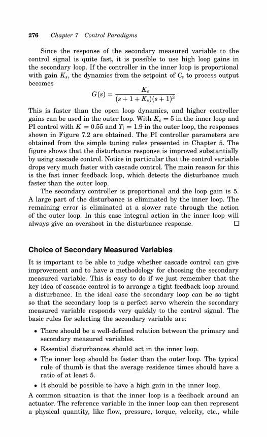
276 Chapter 7 Control Paradigms
Since the response of the secondary measured variable to thecontrol signal is quite fast, it is possible to use high loop gains inthe secondary loop. If the controller in the inner loop is proportionalwith gain Ks, the dynamics from the setpoint of Cs to process outputbecomes
G(s) = Ks
(s+ 1+ Ks)(s+ 1)3This is faster than the open loop dynamics, and higher controllergains can be used in the outer loop. With Ks = 5 in the inner loop andPI control with K = 0.55 and Ti = 1.9 in the outer loop, the responsesshown in Figure 7.2 are obtained. The PI controller parameters areobtained from the simple tuning rules presented in Chapter 5. Thefigure shows that the disturbance response is improved substantiallyby using cascade control. Notice in particular that the control variabledrops very much faster with cascade control. The main reason for thisis the fast inner feedback loop, which detects the disturbance muchfaster than the outer loop.The secondary controller is proportional and the loop gain is 5.
A large part of the disturbance is eliminated by the inner loop. Theremaining error is eliminated at a slower rate through the actionof the outer loop. In this case integral action in the inner loop willalways give an overshoot in the disturbance response.
Choice of Secondary Measured Variables
It is important to be able to judge whether cascade control can giveimprovement and to have a methodology for choosing the secondarymeasured variable. This is easy to do if we just remember that thekey idea of cascade control is to arrange a tight feedback loop arounda disturbance. In the ideal case the secondary loop can be so tightso that the secondary loop is a perfect servo wherein the secondarymeasured variable responds very quickly to the control signal. Thebasic rules for selecting the secondary variable are:
• There should be a well-defined relation between the primary andsecondary measured variables.
• Essential disturbances should act in the inner loop.
• The inner loop should be faster than the outer loop. The typicalrule of thumb is that the average residence times should have aratio of at least 5.
• It should be possible to have a high gain in the inner loop.
A common situation is that the inner loop is a feedback around anactuator. The reference variable in the inner loop can then representa physical quantity, like flow, pressure, torque, velocity, etc., while
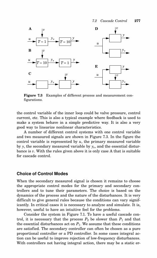
7.2 Cascade Control 277
T = 10 T = 1
ys
ys
ys
T = 10T = 1y
y
y
u
u
u
ys
v
u
y
ys
u
y
vv
v
v
A D
B
C
E
Figure 7.3 Examples of different process and measurement con-figurations.
the control variable of the inner loop could be valve pressure, controlcurrent, etc. This is also a typical example where feedback is used tomake a system behave in a simple predictive way. It is also a verygood way to linearize nonlinear characteristics.A number of different control systems with one control variable
and two measured signals are shown in Figure 7.3. In the figure thecontrol variable is represented by u, the primary measured variableby y, the secondary measured variable by ys, and the essential distur-bance is v. With the rules given above it is only case A that is suitablefor cascade control.
Choice of Control Modes
When the secondary measured signal is chosen it remains to choosethe appropriate control modes for the primary and secondary con-trollers and to tune their parameters. The choice is based on thedynamics of the process and the nature of the disturbances. It is verydifficult to give general rules because the conditions can vary signif-icantly. In critical cases it is necessary to analyze and simulate. It is,however, useful to have an intuitive feel for the problems.Consider the system in Figure 7.1. To have a useful cascade con-
trol, it is necessary that the process P2 be slower than P1 and thatthe essential disturbances act on P1. We assume that these conditionsare satisfied. The secondary controller can often be chosen as a pureproportional controller or a PD controller. In some cases integral ac-tion can be useful to improve rejection of low-frequency disturbances.With controllers not having integral action, there may be a static er-
278 Chapter 7 Control Paradigms
ror in the secondary loop. This may not be a serious drawback. Thesecondary loop, as a rule, is used to eliminate fast disturbances. Slowdisturbances can easily be eliminated by the primary loop, which willtypically have integral action. There are also drawbacks to using in-tegral control in the secondary loop. With such a system there willalways be an overshoot in the response of the primary control loop.Integral action is needed if the process P2 contains essential time de-lays and the process P1 is such that the loop gain in the secondaryloop must be limited.The special case when the process P2 is a pure integrator is quite
common. In this case integral action in the inner loop is equivalent toproportional control in the outer loop. If integral action is used in theinner loop, the proportional action in the outer loop must be reduced.This is a significant disadvantage for the performance of the system.A good remedy is to remove the integrator in the inner loop and toincrease the gain in the outer loop.
Tuning and Commissioning
Cascade controllers must be tuned in a correct sequence. The outerloop should first be put in manual when the inner loop is tuned. Theinner loop should then be put in automatic when tuning the outerloop. The inner loop is often tuned for critical or overcritical dampingor equivalently for a small sensitivity (Ms). If this is not done thereis little margin for using feedback in the outer loop.Commissioning of cascade loops also requires some considera-
tions. The following procedure can be used if we start from scratchwith both controllers in manual mode.
1. Adjust the setpoint of the secondary controller to the value of thesecondary process variable.
2. Set the secondary controller in automatic with internal setpointselected.
3. Adjust the primary controller so that its setpoint is equal to theprocess variable and so that its control signal is equal to thesetpoint of the secondary controller.
4. Switch the secondary controller to external setpoint.
5. Switch the primary controller to automatic mode.
The steps given above are automated to different degrees in differentcontrollers. If the procedure is not done in the right way there will beswitching transients.
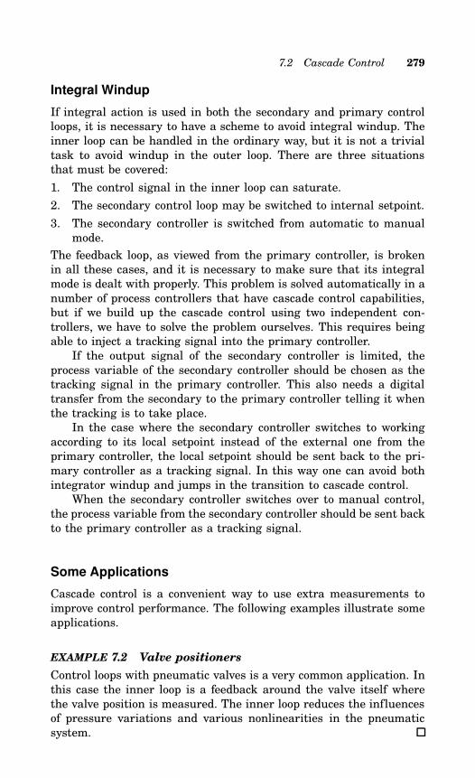
7.2 Cascade Control 279
Integral Windup
If integral action is used in both the secondary and primary controlloops, it is necessary to have a scheme to avoid integral windup. Theinner loop can be handled in the ordinary way, but it is not a trivialtask to avoid windup in the outer loop. There are three situationsthat must be covered:
1. The control signal in the inner loop can saturate.
2. The secondary control loop may be switched to internal setpoint.
3. The secondary controller is switched from automatic to manualmode.
The feedback loop, as viewed from the primary controller, is brokenin all these cases, and it is necessary to make sure that its integralmode is dealt with properly. This problem is solved automatically in anumber of process controllers that have cascade control capabilities,but if we build up the cascade control using two independent con-trollers, we have to solve the problem ourselves. This requires beingable to inject a tracking signal into the primary controller.If the output signal of the secondary controller is limited, the
process variable of the secondary controller should be chosen as thetracking signal in the primary controller. This also needs a digitaltransfer from the secondary to the primary controller telling it whenthe tracking is to take place.In the case where the secondary controller switches to working
according to its local setpoint instead of the external one from theprimary controller, the local setpoint should be sent back to the pri-mary controller as a tracking signal. In this way one can avoid bothintegrator windup and jumps in the transition to cascade control.When the secondary controller switches over to manual control,
the process variable from the secondary controller should be sent backto the primary controller as a tracking signal.
Some Applications
Cascade control is a convenient way to use extra measurements toimprove control performance. The following examples illustrate someapplications.
EXAMPLE 7.2 Valve positioners
Control loops with pneumatic valves is a very common application. Inthis case the inner loop is a feedback around the valve itself wherethe valve position is measured. The inner loop reduces the influencesof pressure variations and various nonlinearities in the pneumaticsystem.
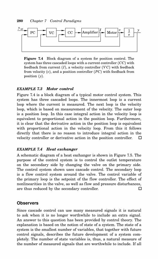
280 Chapter 7 Control Paradigms
Amplifier MotorI v
y sp y1s
CCVCPC
Figure 7.4 Block diagram of a system for position control. Thesystem has three cascaded loops with a current controller (CC) withfeedback from current (I), a velocity controller (VC) with feedbackfrom velocity (v), and a position controller (PC) with feedback fromposition (y).
EXAMPLE 7.3 Motor control
Figure 7.4 is a block diagram of a typical motor control system. Thissystem has three cascaded loops. The innermost loop is a currentloop where the current is measured. The next loop is the velocityloop, which is based on measurement of the velocity. The outer loopis a position loop. In this case integral action in the velocity loop isequivalent to proportional action in the position loop. Furthermore,it is clear that the derivative action in the position loop is equivalentwith proportional action in the velocity loop. From this it followsdirectly that there is no reason to introduce integral action in thevelocity controller or derivative action in the position controller.
EXAMPLE 7.4 Heat exchanger
A schematic diagram of a heat exchanger is shown in Figure 7.5. Thepurpose of the control system is to control the outlet temperatureon the secondary side by changing the valve on the primary side.The control system shown uses cascade control. The secondary loopis a flow control system around the valve. The control variable ofthe primary loop is the setpoint of the flow controller. The effect ofnonlinearities in the valve, as well as flow and pressure disturbances,are thus reduced by the secondary controller.
Observers
Since cascade control can use many measured signals it is naturalto ask when it is no longer worthwhile to include an extra signal.An answer to this question has been provided by control theory. Theexplanation is based on the notion of state of a system. The state of asystem is the smallest number of variables, that together with futurecontrol signals, describes the future development of a system com-pletely. The number of state variables is, thus, a natural measure ofthe number of measured signals that are worthwhile to include. If all
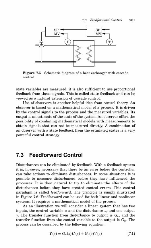
7.3 Feedforward Control 281
SPMV
F
SPMV
T
Figure 7.5 Schematic diagram of a heat exchanger with cascadecontrol.
state variables are measured, it is also sufficient to use proportionalfeedback from these signals. This is called state feedback and can beviewed as a natural extension of cascade control.Use of observers is another helpful idea from control theory. An
observer is based on a mathematical model of a process. It is drivenby the control signals to the process and the measured variables. Itsoutput is an estimate of the state of the system. An observer offers thepossibility of combining mathematical models with measurements toobtain signals that can not be measured directly. A combination ofan observer with a state feedback from the estimated states is a verypowerful control strategy.
7.3 Feedforward Control
Disturbances can be eliminated by feedback. With a feedback systemit is, however, necessary that there be an error before the controllercan take actions to eliminate disturbances. In some situations it ispossible to measure disturbances before they have influenced theprocesses. It is then natural to try to eliminate the effects of thedisturbances before they have created control errors. This controlparadigm is called feedforward. The principle is simply illustratedin Figure 7.6. Feedforward can be used for both linear and nonlinearsystems. It requires a mathematical model of the process.As an illustration we will consider a linear system that has two
inputs, the control variable u and the disturbance v, and one outputy. The transfer function from disturbance to output is Gv, and thetransfer function from the control variable to the output is Gu. Theprocess can be described by the following equation:
Y(s) = Gu(s)U (s) + Gv(s)V (s) (7.1)
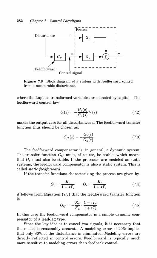
282 Chapter 7 Control Paradigms
Gff
y
v
u
Gu
Gv
Σ
Process
Control signalFeedforward
Disturbance
Figure 7.6 Block diagram of a system with feedforward controlfrom a measurable disturbance.
where the Laplace transformed variables are denoted by capitals. Thefeedforward control law
U (s) = −Gv(s)Gu(s) V (s) (7.2)
makes the output zero for all disturbances v. The feedforward transferfunction thus should be chosen as:
Gf f (s) = −Gv(s)Gu(s) (7.3)
The feedforward compensator is, in general, a dynamic system.The transfer function Gf f must, of course, be stable, which meansthat Gv must also be stable. If the processes are modeled as staticsystems, the feedforward compensator is also a static system. This iscalled static feedforward.If the transfer functions characterizing the process are given by
Gu = Ku
1+ sTu Gv = Kv
1+ sTv (7.4)
it follows from Equation (7.3) that the feedforward transfer functionis
Gf f = − KvKu
⋅1+ sTu1+ sTv (7.5)
In this case the feedforward compensator is a simple dynamic com-pensator of a lead-lag type.Since the key idea is to cancel two signals, it is necessary that
the model is reasonably accurate. A modeling error of 20% impliesthat only 80% of the disturbance is eliminated. Modeling errors aredirectly reflected in control errors. Feedforward is typically muchmore sensitive to modeling errors than feedback control.
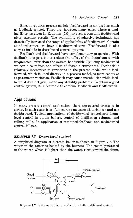
7.3 Feedforward Control 283
Since it requires process models, feedforward is not used as muchas feedback control. There are, however, many cases where a lead-lag filter, as given in Equation (7.5), or even a constant feedforwardgives excellent results. The availability of adaptive techniques hasdrastically increased the range of applicability of feedforward. Certainstandard controllers have a feedforward term. Feedforward is alsoeasy to include in distributed control systems.Feedback and feedforward have complementary properties. With
feedback it is possible to reduce the effect of the disturbances withfrequencies lower than the system bandwidth. By using feedforwardwe can also reduce the effects of faster disturbances. Feedback isrelatively insensitive to variations in the process model while feed-forward, which is used directly in a process model, is more sensitiveto parameter variation. Feedback may cause instabilities while feed-forward does not give rise to any stability problems. To obtain a goodcontrol system, it is desirable to combine feedback and feedforward.
Applications
In many process control applications there are several processes inseries. In such cases it is often easy to measure disturbances and usefeedforward. Typical applications of feedforward control are: drum-level control in steam boilers, control of distillation columns androlling mills. An application of combined feedback and feedforwardcontrol follows.
EXAMPLE 7.5 Drum level control
A simplified diagram of a steam boiler is shown in Figure 7.7. Thewater in the raiser is heated by the burners. The steam generatedin the raiser, which is lighter than the water, rises toward the drum.
F F
L Drum
TurbineOil
Air
Feedwater
Steam valve
Raiser Down comer
Figure 7.7 Schematic diagram of a drum boiler with level control.
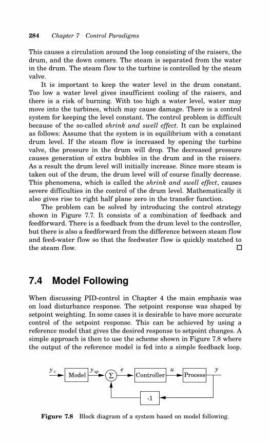
284 Chapter 7 Control Paradigms
This causes a circulation around the loop consisting of the raisers, thedrum, and the down comers. The steam is separated from the waterin the drum. The steam flow to the turbine is controlled by the steamvalve.It is important to keep the water level in the drum constant.
Too low a water level gives insufficient cooling of the raisers, andthere is a risk of burning. With too high a water level, water maymove into the turbines, which may cause damage. There is a controlsystem for keeping the level constant. The control problem is difficultbecause of the so-called shrink and swell effect. It can be explainedas follows: Assume that the system is in equilibrium with a constantdrum level. If the steam flow is increased by opening the turbinevalve, the pressure in the drum will drop. The decreased pressurecauses generation of extra bubbles in the drum and in the raisers.As a result the drum level will initially increase. Since more steam istaken out of the drum, the drum level will of course finally decrease.This phenomena, which is called the shrink and swell effect, causessevere difficulties in the control of the drum level. Mathematically italso gives rise to right half plane zero in the transfer function.The problem can be solved by introducing the control strategy
shown in Figure 7.7. It consists of a combination of feedback andfeedforward. There is a feedback from the drum level to the controller,but there is also a feedforward from the difference between steam flowand feed-water flow so that the feedwater flow is quickly matched tothe steam flow.
7.4 Model Following
When discussing PID-control in Chapter 4 the main emphasis wason load disturbance response. The setpoint response was shaped bysetpoint weighting. In some cases it is desirable to have more accuratecontrol of the setpoint response. This can be achieved by using areference model that gives the desired response to setpoint changes. Asimple approach is then to use the scheme shown in Figure 7.8 wherethe output of the reference model is fed into a simple feedback loop.
uΣModel
e yController
-1
Process y spy c
Figure 7.8 Block diagram of a system based on model following.
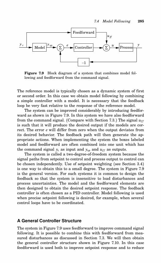
7.4 Model Following 285
y c uΣModel
e y
−1
Processy sp
Feedforward
ΣController
uff
Figure 7.9 Block diagram of a system that combines model fol-lowing and feedforward from the command signal.
The reference model is typically chosen as a dynamic system of firstor second order. In this case we obtain model following by combininga simple controller with a model. It is necessary that the feedbackloop be very fast relative to the response of the reference model.The system can be improved considerably by introducing feedfor-
ward as shown in Figure 7.9. In this system we have also feedforwardfrom the command signal. (Compare with Section 7.3.) The signal uf fis such that it will produce the desired output if the models are cor-rect. The error e will differ from zero when the output deviates fromits desired behavior. The feedback path will then generate the ap-propriate actions. When implementing the system the boxes labeledmodel and feedforward are often combined into one unit which hasthe command signal yc as input and ysp and uf f as outputs.The system is called a two-degree-of-freedom system because the
signal paths from setpoint to control and process output to control canbe chosen independently. Use of setpoint weighting (see Section 3.4)is one way to obtain this to a small degree. The system in Figure 7.9is the general version. For such systems it is common to design thefeedback so that the system is insensitive to load disturbances andprocess uncertainties. The model and the feedforward elements arethen designed to obtain the desired setpoint response. The feedbackcontroller is often chosen as a PID controller. Model following is usedwhen precise setpoint following is desired, for example, when severalcontrol loops have to be coordinated.
A General Controller Structure
The system in Figure 7.9 uses feedforward to improve command signalfollowing. It is possible to combine this with feedforward from mea-sured disturbances as discussed in Section 7.3. We will then obtainthe general controller structure shown in Figure 7.10. In this casefeedforward is used both to improve setpoint response and to reduce
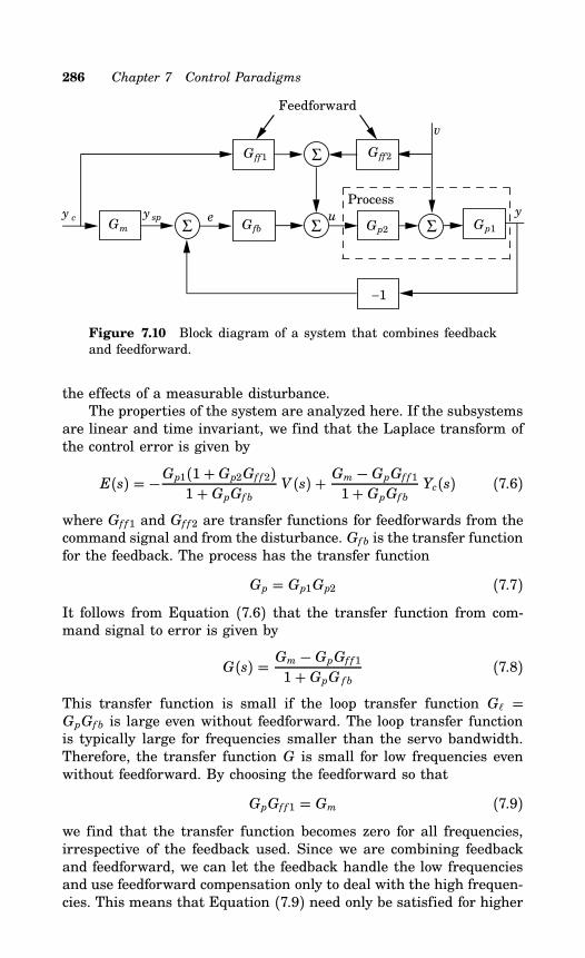
286 Chapter 7 Control Paradigms
yGp1Σ
v
y c e
−1
Process
uΣ
y sp
Feedforward
Σ
ΣGm
Gff2Gff1
Gfb Gp2
Figure 7.10 Block diagram of a system that combines feedbackand feedforward.
the effects of a measurable disturbance.The properties of the system are analyzed here. If the subsystems
are linear and time invariant, we find that the Laplace transform ofthe control error is given by
E(s) = −Gp1(1+ Gp2Gf f2)1+ GpGfb V (s) + Gm − GpGf f1
1+ GpGfb Yc(s) (7.6)
where Gf f1 and Gf f2 are transfer functions for feedforwards from thecommand signal and from the disturbance. Gfb is the transfer functionfor the feedback. The process has the transfer function
Gp = Gp1Gp2 (7.7)It follows from Equation (7.6) that the transfer function from com-mand signal to error is given by
G(s) = Gm − GpGf f11+ GpG fb (7.8)
This transfer function is small if the loop transfer function G =GpGfb is large even without feedforward. The loop transfer functionis typically large for frequencies smaller than the servo bandwidth.Therefore, the transfer function G is small for low frequencies evenwithout feedforward. By choosing the feedforward so that
GpGf f1 = Gm (7.9)we find that the transfer function becomes zero for all frequencies,irrespective of the feedback used. Since we are combining feedbackand feedforward, we can let the feedback handle the low frequenciesand use feedforward compensation only to deal with the high frequen-cies. This means that Equation (7.9) need only be satisfied for higher
7.5 Nonlinear Elements 287
frequencies. This makes the feedforward compensator simpler. Sim-ilarly it follows from Equation (7.6) that the transfer function fromthe disturbance to the control error is given by
Gv = −Gp1(1+ Gp2Gf f2)1+ GpGfbIn an analogy with the previous discussion, we find that this transferfunction will be zero if
Gp2Gf f2 = −1holds. The transfer function will also be small if the loop transferfunction G is large.These simple calculations illustrate the differences between feed-
back and feedforward. In particular they show that feedforward re-duces disturbances by canceling two terms, while feedback reducesthe disturbances by dividing them by a large number. This clearlydemonstrates why feedforward is more sensitive than feedback.
Tuning Feedforward Controllers
Feedforward controllers must be well tuned. Unfortunately, it is dif-ficult to tune such controllers. The main difficulty is that it is oftennot possible to change the disturbances in order to investigate thedisturbance response. Therefore, it is necessary to wait for a nat-ural disturbance before the performance of the feedforward can beobserved. This makes tuning very time consuming.
7.5 Nonlinear Elements
Nonlinear elements have been discussed before. In Section 3.5 we useda limiter to avoid integral windup, in Section 3.4 we discussed the ad-dition of nonlinearities to obtain “error squared on proportional” andsimilar control functions. In Chapter 6 it was shown that performancecould be improved by gain scheduling. In this section we describemore nonlinear elements and also present some control paradigmsthat guide the use of these elements.
Limiters
Since all physical values are limited, it is useful to have limitingdevices in control systems too. A simple amplitude limiter is shownin Figure 7.11. The limiter can mathematically be described as the
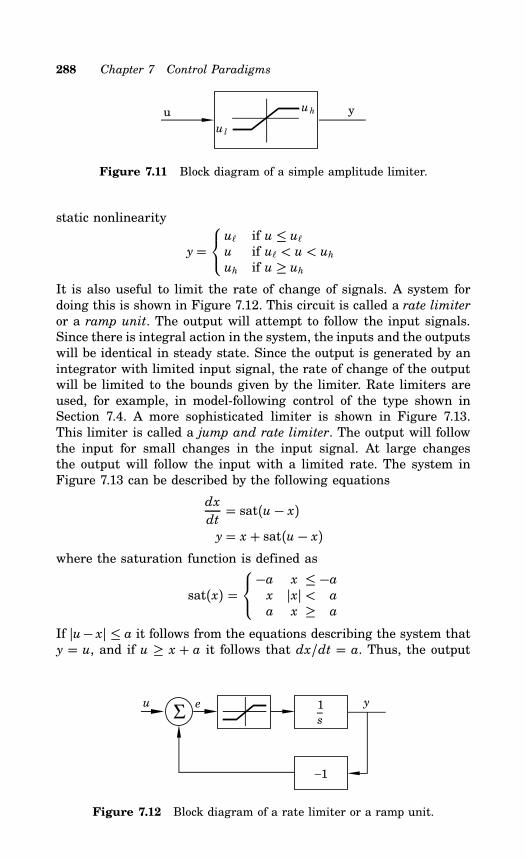
288 Chapter 7 Control Paradigms
ul
uhu y
Figure 7.11 Block diagram of a simple amplitude limiter.
static nonlinearity
y=u if u ≤ uu if u < u < uhuh if u ≥ uh
It is also useful to limit the rate of change of signals. A system fordoing this is shown in Figure 7.12. This circuit is called a rate limiteror a ramp unit. The output will attempt to follow the input signals.Since there is integral action in the system, the inputs and the outputswill be identical in steady state. Since the output is generated by anintegrator with limited input signal, the rate of change of the outputwill be limited to the bounds given by the limiter. Rate limiters areused, for example, in model-following control of the type shown inSection 7.4. A more sophisticated limiter is shown in Figure 7.13.This limiter is called a jump and rate limiter. The output will followthe input for small changes in the input signal. At large changesthe output will follow the input with a limited rate. The system inFigure 7.13 can be described by the following equations
dx
dt= sat(u − x)y = x + sat(u− x)
where the saturation function is defined as
sat(x) =−a x ≤ −ax x < a
a x ≥ a
If u− x ≤ a it follows from the equations describing the system thaty = u, and if u ≥ x + a it follows that dx/dt = a. Thus, the output
yuΣ
1
s
−1
e
Figure 7.12 Block diagram of a rate limiter or a ramp unit.
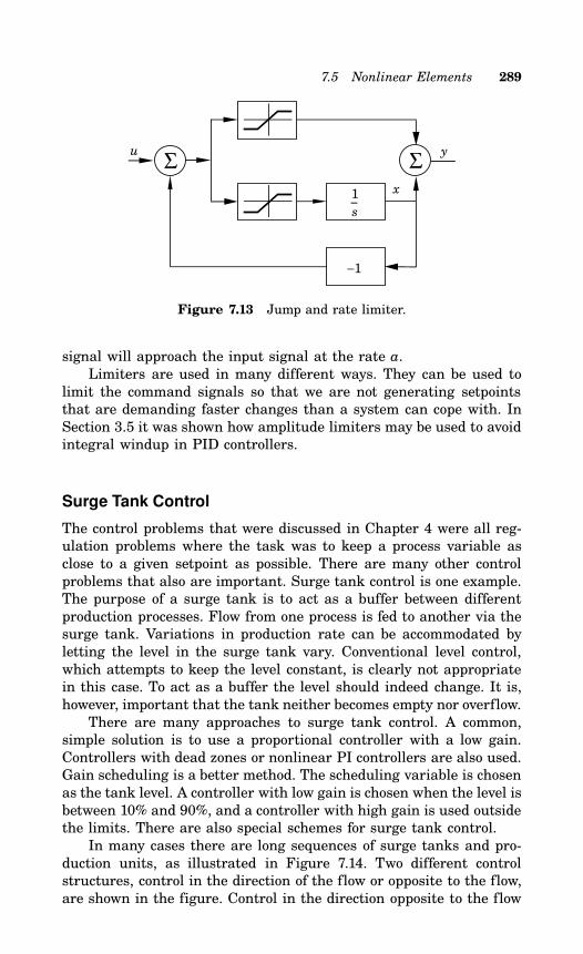
7.5 Nonlinear Elements 289
yΣ
uΣ
1
s
−1
x
Figure 7.13 Jump and rate limiter.
signal will approach the input signal at the rate a.Limiters are used in many different ways. They can be used to
limit the command signals so that we are not generating setpointsthat are demanding faster changes than a system can cope with. InSection 3.5 it was shown how amplitude limiters may be used to avoidintegral windup in PID controllers.
Surge Tank Control
The control problems that were discussed in Chapter 4 were all reg-ulation problems where the task was to keep a process variable asclose to a given setpoint as possible. There are many other controlproblems that also are important. Surge tank control is one example.The purpose of a surge tank is to act as a buffer between differentproduction processes. Flow from one process is fed to another via thesurge tank. Variations in production rate can be accommodated byletting the level in the surge tank vary. Conventional level control,which attempts to keep the level constant, is clearly not appropriatein this case. To act as a buffer the level should indeed change. It is,however, important that the tank neither becomes empty nor overflow.There are many approaches to surge tank control. A common,
simple solution is to use a proportional controller with a low gain.Controllers with dead zones or nonlinear PI controllers are also used.Gain scheduling is a better method. The scheduling variable is chosenas the tank level. A controller with low gain is chosen when the level isbetween 10% and 90%, and a controller with high gain is used outsidethe limits. There are also special schemes for surge tank control.In many cases there are long sequences of surge tanks and pro-
duction units, as illustrated in Figure 7.14. Two different controlstructures, control in the direction of the flow or opposite to the flow,are shown in the figure. Control in the direction opposite to the flow
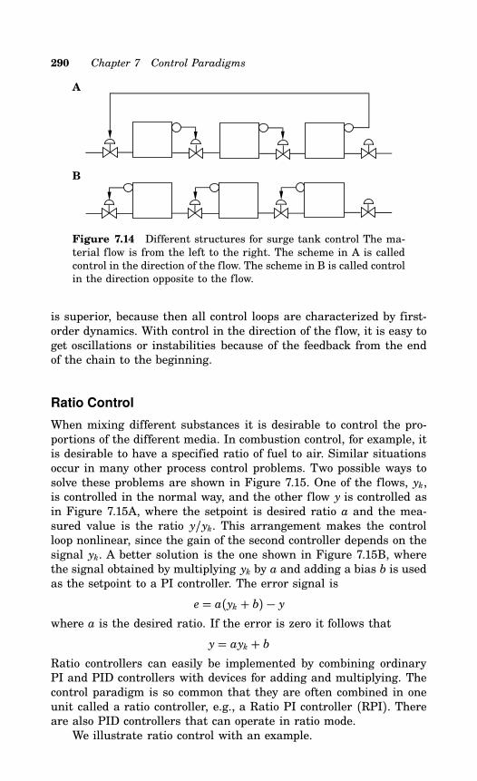
290 Chapter 7 Control Paradigms
A
B
Figure 7.14 Different structures for surge tank control The ma-terial flow is from the left to the right. The scheme in A is calledcontrol in the direction of the flow. The scheme in B is called controlin the direction opposite to the flow.
is superior, because then all control loops are characterized by first-order dynamics. With control in the direction of the flow, it is easy toget oscillations or instabilities because of the feedback from the endof the chain to the beginning.
Ratio Control
When mixing different substances it is desirable to control the pro-portions of the different media. In combustion control, for example, itis desirable to have a specified ratio of fuel to air. Similar situationsoccur in many other process control problems. Two possible ways tosolve these problems are shown in Figure 7.15. One of the flows, yk,is controlled in the normal way, and the other flow y is controlled asin Figure 7.15A, where the setpoint is desired ratio a and the mea-sured value is the ratio y/yk. This arrangement makes the controlloop nonlinear, since the gain of the second controller depends on thesignal yk. A better solution is the one shown in Figure 7.15B, wherethe signal obtained by multiplying yk by a and adding a bias b is usedas the setpoint to a PI controller. The error signal is
e = a(yk + b) − ywhere a is the desired ratio. If the error is zero it follows that
y= ayk + bRatio controllers can easily be implemented by combining ordinaryPI and PID controllers with devices for adding and multiplying. Thecontrol paradigm is so common that they are often combined in oneunit called a ratio controller, e.g., a Ratio PI controller (RPI). Thereare also PID controllers that can operate in ratio mode.We illustrate ratio control with an example.
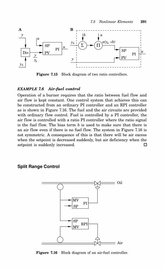
7.5 Nonlinear Elements 291
a(yk +b)Σ
ykΠ
y
PISP
PV
u
b aa
yk
y
Divy
PISP
PV
u
ky
A B
Figure 7.15 Block diagram of two ratio controllers.
EXAMPLE 7.6 Air-fuel control
Operation of a burner requires that the ratio between fuel flow andair flow is kept constant. One control system that achieves this canbe constructed from an ordinary PI controller and an RPI controlleras is shown in Figure 7.16. The fuel and the air circuits are providedwith ordinary flow control. Fuel is controlled by a PI controller, theair flow is controlled with a ratio PI controller where the ratio signalis the fuel flow. The bias term b is used to make sure that there isan air flow even if there is no fuel flow. The system in Figure 7.16 isnot symmetric. A consequence of this is that there will be air excesswhen the setpoint is decreased suddenly, but air deficiency when thesetpoint is suddenly increased.
Split Range Control
SP
MVRPI
MV
SPPI
Oil
Air
Figure 7.16 Block diagram of an air-fuel controller.
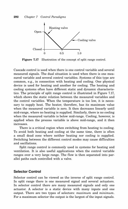
292 Chapter 7 Control Paradigms
Open
Closed
0 0.5 1.0
Cooling valve
Heating valve
Figure 7.17 Illustration of the concept of split range control.
Cascade control is used when there is one control variable and severalmeasured signals. The dual situation is used when there is one mea-sured variable and several control variables. Systems of this type arecommon, e.g., in connection with heating and cooling. One physicaldevice is used for heating and another for cooling. The heating andcooling systems often have different static and dynamic characteris-tics. The principle of split range control is illustrated in Figure 7.17,which shows the static relation between the measured variables andthe control variables. When the temperature is too low, it is neces-sary to supply heat. The heater, therefore, has its maximum valuewhen the measured variable is zero. It then decreases linearly untilmid-range, where no heating is supplied. Similarly, there is no coolingwhen the measured variable is below mid-range. Cooling, however, isapplied when the process variable is above mid-range, and it thenincreases.There is a critical region when switching from heating to cooling.
To avoid both heating and cooling at the same time, there is oftena small dead zone where neither heating nor cooling is supplied.Switching between the different control modes may cause difficultiesand oscillations.Split range control is commonly used in systems for heating and
ventilation. It is also useful applications when the control variableranges over a very large range. The flow is then separated into par-allel paths each controlled with a valve.
Selector Control
Selector control can be viewed as the inverse of split range control.In split range there is one measured signal and several actuators.In selector control there are many measured signals and only oneactuator. A selector is a static device with many inputs and oneoutput. There are two types of selectors: maximum and minimum.For a maximum selector the output is the largest of the input signals.
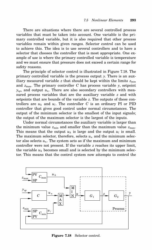
7.5 Nonlinear Elements 293
There are situations where there are several controlled processvariables that must be taken into account. One variable is the pri-mary controlled variable, but it is also required that other processvariables remain within given ranges. Selector control can be usedto achieve this. The idea is to use several controllers and to have aselector that chooses the controller that is most appropriate. One ex-ample of use is where the primary controlled variable is temperatureand we must ensure that pressure does not exceed a certain range forsafety reasons.The principle of selector control is illustrated in Figure 7.18. The
primary controlled variable is the process output y. There is an aux-iliary measured variable z that should be kept within the limits zminand zmax. The primary controller C has process variable y, setpointysp, and output un. There are also secondary controllers with mea-sured process variables that are the auxiliary variable z and withsetpoints that are bounds of the variable z. The outputs of these con-trollers are uh and ul . The controller C is an ordinary PI or PIDcontroller that gives good control under normal circumstances. Theoutput of the minimum selector is the smallest of the input signals;the output of the maximum selector is the largest of the inputs.Under normal circumstances the auxiliary variable is larger than
the minimum value zmin and smaller than the maximum value zmax.This means that the output uh is large and the output ul is small.The maximum selector, therefore, selects un and the minimum selec-tor also selects un. The system acts as if the maximum and minimumcontroller were not present. If the variable z reaches its upper limit,the variable uh becomes small and is selected by the minimum selec-tor. This means that the control system now attempts to control the
MAX
MIN
Cmin
Cmax
C
u l
zmin
zmax
y
u h
Process
u zG2G1
u n
SP
PV
ysp
SP
PV
Figure 7.18 Selector control.
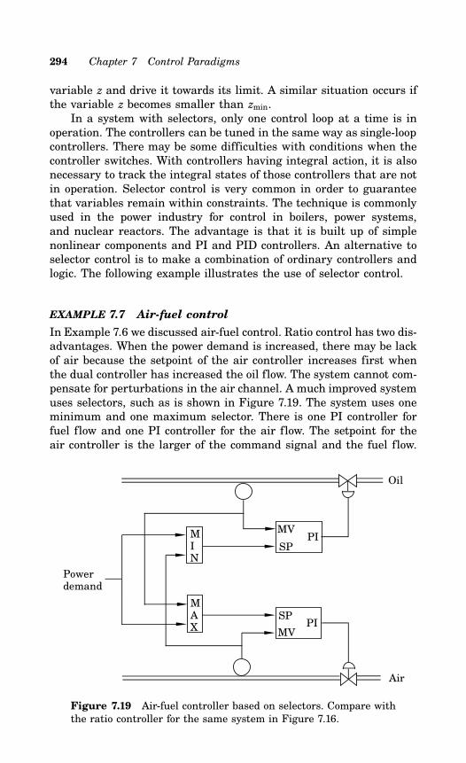
294 Chapter 7 Control Paradigms
variable z and drive it towards its limit. A similar situation occurs ifthe variable z becomes smaller than zmin.In a system with selectors, only one control loop at a time is in
operation. The controllers can be tuned in the same way as single-loopcontrollers. There may be some difficulties with conditions when thecontroller switches. With controllers having integral action, it is alsonecessary to track the integral states of those controllers that are notin operation. Selector control is very common in order to guaranteethat variables remain within constraints. The technique is commonlyused in the power industry for control in boilers, power systems,and nuclear reactors. The advantage is that it is built up of simplenonlinear components and PI and PID controllers. An alternative toselector control is to make a combination of ordinary controllers andlogic. The following example illustrates the use of selector control.
EXAMPLE 7.7 Air-fuel control
In Example 7.6 we discussed air-fuel control. Ratio control has two dis-advantages. When the power demand is increased, there may be lackof air because the setpoint of the air controller increases first whenthe dual controller has increased the oil flow. The system cannot com-pensate for perturbations in the air channel. A much improved systemuses selectors, such as is shown in Figure 7.19. The system uses oneminimum and one maximum selector. There is one PI controller forfuel flow and one PI controller for the air flow. The setpoint for theair controller is the larger of the command signal and the fuel flow.
MAX
MIN
SP
MVPI
MV
SPPI
Oil
Air
Powerdemand
Figure 7.19 Air-fuel controller based on selectors. Compare withthe ratio controller for the same system in Figure 7.16.
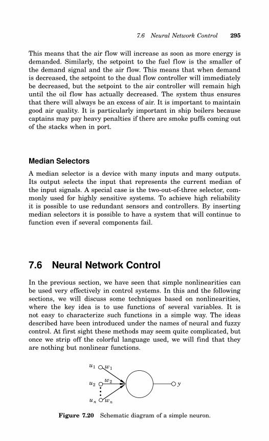
7.6 Neural Network Control 295
This means that the air flow will increase as soon as more energy isdemanded. Similarly, the setpoint to the fuel flow is the smaller ofthe demand signal and the air flow. This means that when demandis decreased, the setpoint to the dual flow controller will immediatelybe decreased, but the setpoint to the air controller will remain highuntil the oil flow has actually decreased. The system thus ensuresthat there will always be an excess of air. It is important to maintaingood air quality. It is particularly important in ship boilers becausecaptains may pay heavy penalties if there are smoke puffs coming outof the stacks when in port.
Median Selectors
A median selector is a device with many inputs and many outputs.Its output selects the input that represents the current median ofthe input signals. A special case is the two-out-of-three selector, com-monly used for highly sensitive systems. To achieve high reliabilityit is possible to use redundant sensors and controllers. By insertingmedian selectors it is possible to have a system that will continue tofunction even if several components fail.
7.6 Neural Network Control
In the previous section, we have seen that simple nonlinearities canbe used very effectively in control systems. In this and the followingsections, we will discuss some techniques based on nonlinearities,where the key idea is to use functions of several variables. It isnot easy to characterize such functions in a simple way. The ideasdescribed have been introduced under the names of neural and fuzzycontrol. At first sight these methods may seem quite complicated, butonce we strip off the colorful language used, we will find that theyare nothing but nonlinear functions.
u1
u2
un
w1
w2
wn
y
Figure 7.20 Schematic diagram of a simple neuron.
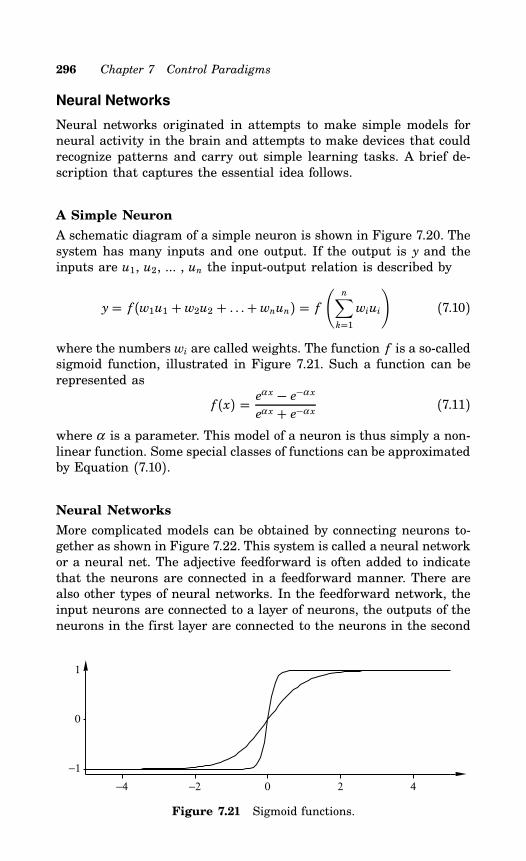
296 Chapter 7 Control Paradigms
Neural Networks
Neural networks originated in attempts to make simple models forneural activity in the brain and attempts to make devices that couldrecognize patterns and carry out simple learning tasks. A brief de-scription that captures the essential idea follows.
A Simple Neuron
A schematic diagram of a simple neuron is shown in Figure 7.20. Thesystem has many inputs and one output. If the output is y and theinputs are u1, u2, ... , un the input-output relation is described by
y= f (w1u1 +w2u2 + . . .+wnun) = f(n∑k=1wiui
)(7.10)
where the numbers wi are called weights. The function f is a so-calledsigmoid function, illustrated in Figure 7.21. Such a function can berepresented as
f (x) = eα x − e−α x
eα x + e−α x(7.11)
where α is a parameter. This model of a neuron is thus simply a non-linear function. Some special classes of functions can be approximatedby Equation (7.10).
Neural Networks
More complicated models can be obtained by connecting neurons to-gether as shown in Figure 7.22. This system is called a neural networkor a neural net. The adjective feedforward is often added to indicatethat the neurons are connected in a feedforward manner. There arealso other types of neural networks. In the feedforward network, theinput neurons are connected to a layer of neurons, the outputs of theneurons in the first layer are connected to the neurons in the second
−4 −2 0 2 4
−1
0
1
Figure 7.21 Sigmoid functions.
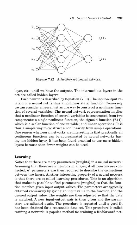
7.6 Neural Network Control 297
u1
u2 y1
y2
u5
u4
u3
Figure 7.22 A feedforward neural network.
layer, etc., until we have the outputs. The intermediate layers in thenet are called hidden layers.Each neuron is described by Equation (7.10). The input-output re-
lation of a neural net is thus a nonlinear static function. Converselywe can consider a neural net as one way to construct a nonlinear func-tion of several variables. The neural network representation impliesthat a nonlinear function of several variables is constructed from twocomponents: a single nonlinear function, the sigmoid function (7.11),which is a scalar function of one variable; and linear operations. It isthus a simple way to construct a nonlinearity from simple operations.One reason why neural networks are interesting is that practically allcontinuous functions can be approximated by neural networks hav-ing one hidden layer. It has been found practical to use more hiddenlayers because then fewer weights can be used.
Learning
Notice that there are many parameters (weights) in a neural network.Assuming that there are n neurons in a layer, if all neurons are con-nected, n2 parameters are then required to describe the connectionsbetween two layers. Another interesting property of a neural networkis that there are so-called learning procedures. This is an algorithmthat makes it possible to find parameters (weights) so that the func-tion matches given input-output values. The parameters are typicallyobtained recursively by giving an input value to the function and thedesired output value. The weights are then adjusted so that the datais matched. A new input-output pair is then given and the param-eters are adjusted again. The procedure is repeated until a good fithas been obtained for a reasonable data set. This procedure is calledtraining a network. A popular method for training a feedforward net-
298 Chapter 7 Control Paradigms
work is called back propagation. For this reason the feedforward netis sometimes called a back-propagation network.
Control Applications
A feedforward neural network is nothing but a nonlinear function ofseveral variables with a training procedure. The function has manyparameters (weights) that can be adjusted by the training procedureso that the function will match given data. Even if this is an extremelysimplistic model of a real neuron, it is a very useful system compo-nent. In process control we can often make good use of nonlinearfunctions. Sensor calibration is one case. There are many situationswhere an instrument has many different sensors, the outputs of whichmust be combined nonlinearly to obtain the desired measured value.Nonlinear functions can also be used for pattern recognition.
7.7 Fuzzy Control
Fuzzy control is an old control paradigm that has received a lot ofattention recently. In this section we will give a brief description ofthe key ideas. We will start with fuzzy logic, which has inspired thedevelopment.
Fuzzy Logic
Ordinary Boolean logic deals with quantities that are either true orfalse. Fuzzy logic is an attempt to develop a method for logic reasoningthat is less sharp. This is achieved by introducing linguistic variablesand associating them with membership functions, which take valuesbetween 0 and 1. In fuzzy control the logical operations and, or, andnot are operations on linguistic variables. These operations can beexpressed in terms of operations on the membership functions ofthe linguistic variables. Consider two linguistic variables with themembership functions fA(x) and fB(x). The logical operations aredefined by the following operations on the membership functions.
fA and B = min ( fA(x), fB(x))fA or B = max ( fA(x), fB(x))fnot A = 1− fA(x)
A linguistic variable, where the membership function is zero every-where except for one particular value, is called a crisp variable.Assume for example that we want to reason about temperature.
For this purpose we introduce the linguistic variables cold, moderate,
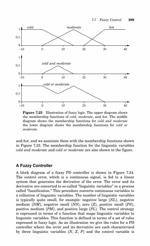
7.7 Fuzzy Control 299
−10 0 10 20 30 400
0.5
1
−10 0 10 20 30 400
0.5
1
−10 0 10 20 30 400
0.5
1
cold moderate hot
cold and moderate
cold or moderate
Figure 7.23 Illustration of fuzzy logic. The upper diagram showsthe membership functions of cold, moderate, and hot. The middlediagram shows the membership functions for cold and moderatethe lower diagram shows the membership functions for cold ormoderate.
and hot, and we associate them with the membership functions shownin Figure 7.23. The membership function for the linguistic variablescold and moderate and cold or moderate are also shown in the figure.
A Fuzzy Controller
A block diagram of a fuzzy PD controller is shown in Figure 7.24.The control error, which is a continuous signal, is fed to a linearsystem that generates the derivative of the error. The error and itsderivative are converted to so-called “linguistic variables” in a processcalled “fuzzification.” This procedure converts continuous variables toa collection of linguistic variables. The number of linguistic variablesis typically quite small, for example: negative large (NL), negativemedium (NM), negative small (NS), zero (Z), positive small (PS),positive medium (PM), and positive large (PL). The control strategyis expressed in terms of a function that maps linguistic variables tolinguistic variables. This function is defined in terms of a set of rulesexpressed in fuzzy logic. As an illustration we give the rules for a PDcontroller where the error and its derivative are each characterizedby three linguistic variables (N, Z, P) and the control variable is
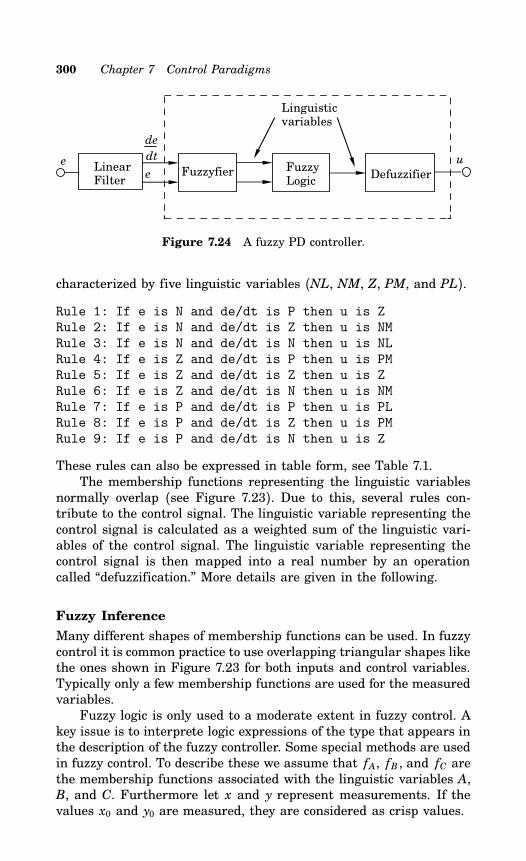
300 Chapter 7 Control Paradigms
FuzzyfierLinearFilter
Fuzzy Logic
Defuzzifier
Linguistic variables
de
dtee
u
Figure 7.24 A fuzzy PD controller.
characterized by five linguistic variables (NL, NM, Z, PM, and PL).Rule 1: If e is N and de/dt is P then u is ZRule 2: If e is N and de/dt is Z then u is NMRule 3: If e is N and de/dt is N then u is NLRule 4: If e is Z and de/dt is P then u is PMRule 5: If e is Z and de/dt is Z then u is ZRule 6: If e is Z and de/dt is N then u is NMRule 7: If e is P and de/dt is P then u is PLRule 8: If e is P and de/dt is Z then u is PMRule 9: If e is P and de/dt is N then u is Z
These rules can also be expressed in table form, see Table 7.1.The membership functions representing the linguistic variables
normally overlap (see Figure 7.23). Due to this, several rules con-tribute to the control signal. The linguistic variable representing thecontrol signal is calculated as a weighted sum of the linguistic vari-ables of the control signal. The linguistic variable representing thecontrol signal is then mapped into a real number by an operationcalled “defuzzification.” More details are given in the following.
Fuzzy Inference
Many different shapes of membership functions can be used. In fuzzycontrol it is common practice to use overlapping triangular shapes likethe ones shown in Figure 7.23 for both inputs and control variables.Typically only a few membership functions are used for the measuredvariables.Fuzzy logic is only used to a moderate extent in fuzzy control. A
key issue is to interprete logic expressions of the type that appears inthe description of the fuzzy controller. Some special methods are usedin fuzzy control. To describe these we assume that fA, fB , and fC arethe membership functions associated with the linguistic variables A,B, and C. Furthermore let x and y represent measurements. If thevalues x0 and y0 are measured, they are considered as crisp values.
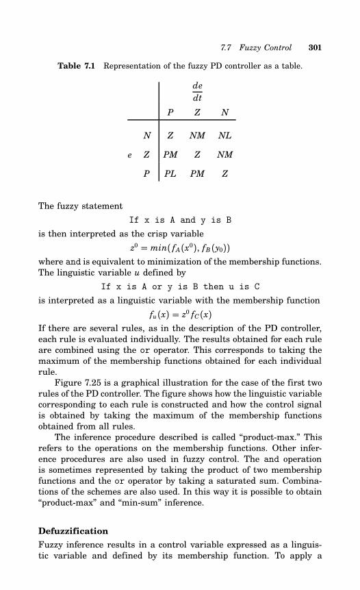
7.7 Fuzzy Control 301
Table 7.1 Representation of the fuzzy PD controller as a table.
de
dt
P Z N
N Z NM NL
e Z PM Z NM
P PL PM Z
The fuzzy statement
If x is A and y is B
is then interpreted as the crisp variable
z0 = min( fA(x0), fB(y0))where and is equivalent to minimization of the membership functions.The linguistic variable u defined by
If x is A or y is B then u is C
is interpreted as a linguistic variable with the membership function
fu(x) = z0 fC(x)If there are several rules, as in the description of the PD controller,each rule is evaluated individually. The results obtained for each ruleare combined using the or operator. This corresponds to taking themaximum of the membership functions obtained for each individualrule.Figure 7.25 is a graphical illustration for the case of the first two
rules of the PD controller. The figure shows how the linguistic variablecorresponding to each rule is constructed and how the control signalis obtained by taking the maximum of the membership functionsobtained from all rules.The inference procedure described is called “product-max.” This
refers to the operations on the membership functions. Other infer-ence procedures are also used in fuzzy control. The and operationis sometimes represented by taking the product of two membershipfunctions and the or operator by taking a saturated sum. Combina-tions of the schemes are also used. In this way it is possible to obtain“product-max” and “min-sum” inference.
Defuzzification
Fuzzy inference results in a control variable expressed as a linguis-tic variable and defined by its membership function. To apply a
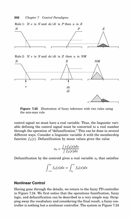
302 Chapter 7 Control Paradigms
Rule 1: If e is N and de/dt is P then u is Z
Rule 2: If e is N and de/dt is Z then u is NM
N
N
P
Z
Z
NM
e de
dt
Figure 7.25 Illustration of fuzzy inference with two rules usingthe min-max rule.
control signal we must have a real variable. Thus, the linguistic vari-able defining the control signal must be converted to a real numberthrough the operation of “defuzzification.” This can be done in severaldifferent ways. Consider a linguistic variable A with the membershipfunction fA(x). Defuzzification by mean values gives the value
x0 =∫x fA(x)dx∫fA(x)dx
Defuzzification by the centroid gives a real variable x0 that satisfies∫ x0
−∞fA(x)dx =
∫ ∞
x0
fA(x)dx
Nonlinear Control
Having gone through the details, we return to the fuzzy PD controllerin Figure 7.24. We first notice that the operations fuzzification, fuzzylogic, and defuzzification can be described in a very simple way. Strip-ping away the vocabulary and considering the final result, a fuzzy con-troller is nothing but a nonlinear controller. The system in Figure 7.24
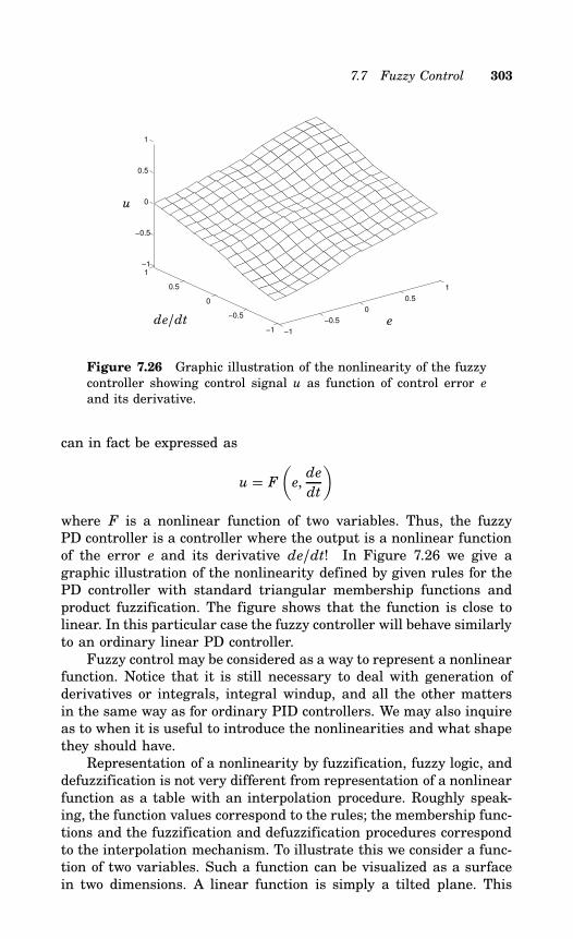
7.7 Fuzzy Control 303
−1
−0.5
0
0.5
1
−1
−0.5
0
0.5
1−1
−0.5
0
0.5
1
u
de/dt e
Figure 7.26 Graphic illustration of the nonlinearity of the fuzzycontroller showing control signal u as function of control error eand its derivative.
can in fact be expressed as
u = F(e,de
dt
)
where F is a nonlinear function of two variables. Thus, the fuzzyPD controller is a controller where the output is a nonlinear functionof the error e and its derivative de/dt! In Figure 7.26 we give agraphic illustration of the nonlinearity defined by given rules for thePD controller with standard triangular membership functions andproduct fuzzification. The figure shows that the function is close tolinear. In this particular case the fuzzy controller will behave similarlyto an ordinary linear PD controller.Fuzzy control may be considered as a way to represent a nonlinear
function. Notice that it is still necessary to deal with generation ofderivatives or integrals, integral windup, and all the other mattersin the same way as for ordinary PID controllers. We may also inquireas to when it is useful to introduce the nonlinearities and what shapethey should have.Representation of a nonlinearity by fuzzification, fuzzy logic, and
defuzzification is not very different from representation of a nonlinearfunction as a table with an interpolation procedure. Roughly speak-ing, the function values correspond to the rules; the membership func-tions and the fuzzification and defuzzification procedures correspondto the interpolation mechanism. To illustrate this we consider a func-tion of two variables. Such a function can be visualized as a surfacein two dimensions. A linear function is simply a tilted plane. This
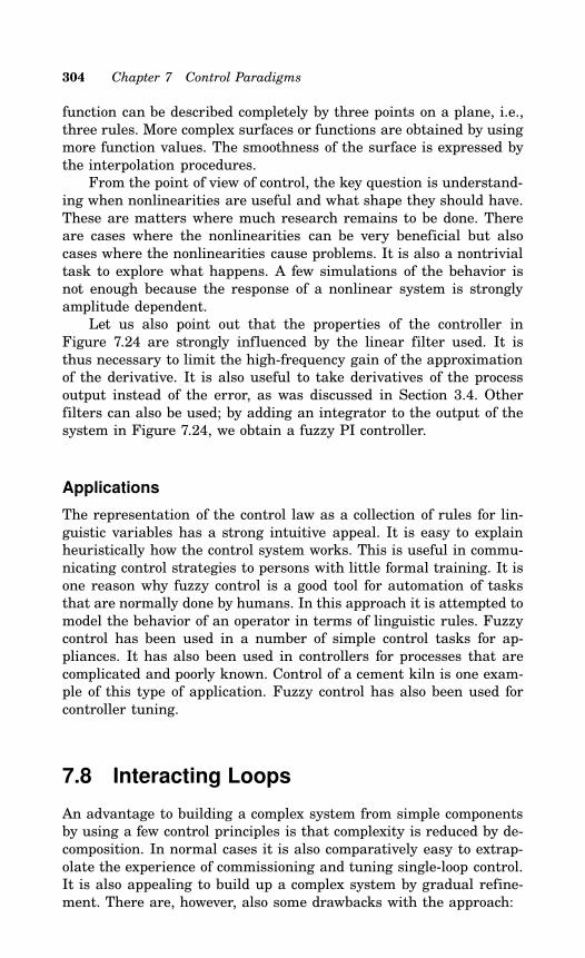
304 Chapter 7 Control Paradigms
function can be described completely by three points on a plane, i.e.,three rules. More complex surfaces or functions are obtained by usingmore function values. The smoothness of the surface is expressed bythe interpolation procedures.From the point of view of control, the key question is understand-
ing when nonlinearities are useful and what shape they should have.These are matters where much research remains to be done. Thereare cases where the nonlinearities can be very beneficial but alsocases where the nonlinearities cause problems. It is also a nontrivialtask to explore what happens. A few simulations of the behavior isnot enough because the response of a nonlinear system is stronglyamplitude dependent.Let us also point out that the properties of the controller in
Figure 7.24 are strongly influenced by the linear filter used. It isthus necessary to limit the high-frequency gain of the approximationof the derivative. It is also useful to take derivatives of the processoutput instead of the error, as was discussed in Section 3.4. Otherfilters can also be used; by adding an integrator to the output of thesystem in Figure 7.24, we obtain a fuzzy PI controller.
Applications
The representation of the control law as a collection of rules for lin-guistic variables has a strong intuitive appeal. It is easy to explainheuristically how the control system works. This is useful in commu-nicating control strategies to persons with little formal training. It isone reason why fuzzy control is a good tool for automation of tasksthat are normally done by humans. In this approach it is attempted tomodel the behavior of an operator in terms of linguistic rules. Fuzzycontrol has been used in a number of simple control tasks for ap-pliances. It has also been used in controllers for processes that arecomplicated and poorly known. Control of a cement kiln is one exam-ple of this type of application. Fuzzy control has also been used forcontroller tuning.
7.8 Interacting Loops
An advantage to building a complex system from simple componentsby using a few control principles is that complexity is reduced by de-composition. In normal cases it is also comparatively easy to extrap-olate the experience of commissioning and tuning single-loop control.It is also appealing to build up a complex system by gradual refine-ment. There are, however, also some drawbacks with the approach:
7.8 Interacting Loops 305
• Since we have not determined the fundamental limitations, itis difficult to decide when further refinements do not give anysignificant benefits.
• It is easy to get systems that are unnecessarily complicated. Wemay get systems where several control loops are fighting eachother.
• There are cases where it is difficult to arrive at a good overallsystem by a loop-by-loop approach.
If there are difficulties, it is necessary to use a systematic approachbased on mathematical modeling analysis and simulation. This is,however, more demanding than the empirical approach. In this sectionwe illustrate some of the difficulties that may arise.
Parallel Systems
Systems that are connected in parallel are quite common. Typicalexamples are motors that are driving the same load, power systemsand networks for steam distribution. Control of such systems requirespecial consideration. To illustrate the difficulties that may arise wewill consider the situation with two motors driving the same load. Aschematic diagram of the system is shown in Figure 7.27.Let ω be the angular velocity of the shaft, J the total moment
of inertia, and D the damping coefficient. The system can then bedescribed by the equation
Jdω
dt+ Dω = M1 + M2 − ML (7.12)
where M1 and M2 are the torques from the motors and ML is the loadtorque.
ω wsp
A1
A2 C2
C1
Gearbox
Figure 7.27 Schematic diagram of two motors that drive the sameload.
306 Chapter 7 Control Paradigms
Proportional Control
Assume each motor is provided with a proportional controller. Thecontrol strategies are then
M1 = M10 + K1(ω sp −ω )M2 = M20 + K2(ω sp −ω ) (7.13)
In these equations the parameters M10 and M20 give the torques pro-vided by each motor when ω = ω sp and K1 and K2 are the controllergains. It follows from Equations (7.12) and (7.13) that
Jdω
dt+ (D + K1 + K2)ω = M10 + M20 − ML + (K1 + K2)ω sp
The closed-loop system is, thus, a dynamical system of first order.After perturbations the angular velocity reaches its steady state witha time constant
T = J
D + K1 + K2The response speed is thus given by the sum of the damping and thecontroller gains. The stationary value of the angular velocity is givenby
ω = ω 0 = K1 + K2D + K1 + K2 ω sp + M10 +M20 − ML
D + K1 + K2This implies that there normally will be a steady state error. Similarlywe find from Equation (7.13) that
M1 − M10M2 − M20 =
K1
K2
The ratio of the controller gains will indicate how the load is sharedbetween the motors.
Proportional and Integral Control
The standard way to eliminate a steady state error is to introduceintegral action. In Figure 7.28 we show a simulation of the systemin which the motors have identical PI controllers. The setpoint ischanged at time 0. A load disturbance in the form of a step in theload torque is introduced at time 10 and a pulse-like measurementdisturbance in the second motor controller is introduced at time 20.When the measurement error occurs the balance of the torques ischanged so that the first motor takes up much more of the load afterthe disturbance. In this particular case the second motor is actuallybreaking. This is highly undesirable, of course.To understand the phenomena we show the block diagram of the
system in Figure 7.29. The figure shows that there are two parallel
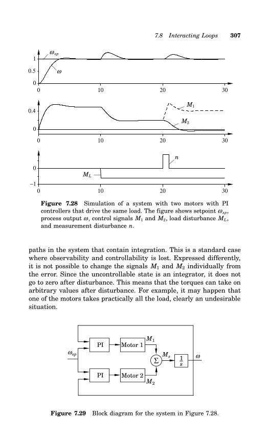
7.8 Interacting Loops 307
0 10 20 300
0.5
1
0 10 20 30
0
0.4
0 10 20 30−1
0
ω sp
ω
M1
M2
n
ML
Figure 7.28 Simulation of a system with two motors with PIcontrollers that drive the same load. The figure shows setpoint ω sp,process output ω , control signals M1 and M2, load disturbance ML,and measurement disturbance n.
paths in the system that contain integration. This is a standard casewhere observability and controllability is lost. Expressed differently,it is not possible to change the signals M1 and M2 individually fromthe error. Since the uncontrollable state is an integrator, it does notgo to zero after disturbance. This means that the torques can take onarbitrary values after disturbance. For example, it may happen thatone of the motors takes practically all the load, clearly an undesirablesituation.
M1
M2
PI
PI
Σ Ms ω
Motor 2
Motor 1
1s
ωsp
Figure 7.29 Block diagram for the system in Figure 7.28.
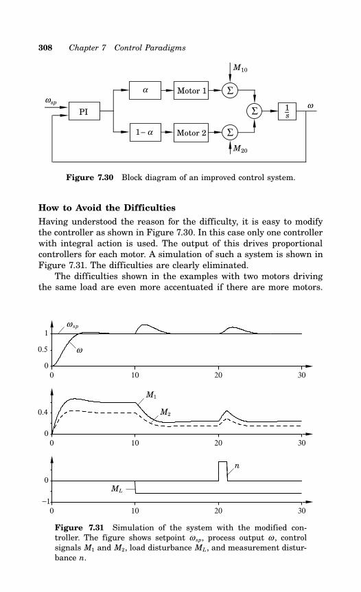
308 Chapter 7 Control Paradigms
1− α
α
ωsp
Σ
M20
Σ
M10
ΣPIω
Motor 1
Motor 2
1s
Figure 7.30 Block diagram of an improved control system.
How to Avoid the Difficulties
Having understood the reason for the difficulty, it is easy to modifythe controller as shown in Figure 7.30. In this case only one controllerwith integral action is used. The output of this drives proportionalcontrollers for each motor. A simulation of such a system is shown inFigure 7.31. The difficulties are clearly eliminated.The difficulties shown in the examples with two motors driving
the same load are even more accentuated if there are more motors.
0 10 20 300
0.5
1
0 10 20 300
0.4
0 10 20 30−1
0
ω sp
ω
M1
M2
n
ML
Figure 7.31 Simulation of the system with the modified con-troller. The figure shows setpoint ω sp, process output ω , controlsignals M1 and M2, load disturbance ML, and measurement distur-bance n.
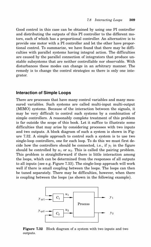
7.8 Interacting Loops 309
Good control in this case can be obtained by using one PI controllerand distributing the outputs of this PI controller to the different mo-tors, each of which has a proportional controller. An alternative is toprovide one motor with a PI controller and let the other have propor-tional control. To summarize, we have found that there may be diffi-culties with parallel systems having integral action. The difficultiesare caused by the parallel connection of integrators that produce un-stable subsystems that are neither controllable nor observable. Withdisturbances these modes can change in an arbitrary manner. Theremedy is to change the control strategies so there is only one inte-grator.
Interaction of Simple Loops
There are processes that have many control variables and many mea-sured variables. Such systems are called multi-input multi-output(MIMO) systems. Because of the interaction between the signals, itmay be very difficult to control such systems by a combination ofsimple controllers. A reasonably complete treatment of this problemis far outside the scope of this book. Let it suffice to illustrate somedifficulties that may arise by considering processes with two inputsand two outputs. A block diagram of such a system is shown in Fig-ure 7.32. A simple approach to control such a system is to use twosingle-loop controllers, one for each loop. To do this we must first de-cide how the controllers should be connected, i.e., if y1 in the figureshould be controlled by u1 or u2. This is called the pairing problem.This problem is straightforward if there is little interaction amongthe loops, which can be determined from the responses of all outputsto all inputs (see e.g. Figure 7.33). The single-loop approach will workwell if there is small coupling between the loops. The loops can thenbe tuned separately. There may be difficulties, however, when thereis coupling between the loops (as shown in the following example).
Process
y1
y2
C1
C2
y sp1
y sp2
u2
u1
Figure 7.32 Block diagram of a system with two inputs and twooutputs.
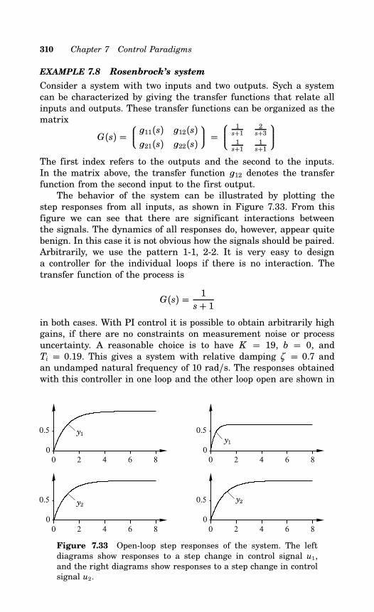
310 Chapter 7 Control Paradigms
EXAMPLE 7.8 Rosenbrock’s system
Consider a system with two inputs and two outputs. Sych a systemcan be characterized by giving the transfer functions that relate allinputs and outputs. These transfer functions can be organized as thematrix
G(s) =11(s) 12(s)21(s) 22(s)
= 1s+1
2s+3
1s+1
1s+1
The first index refers to the outputs and the second to the inputs.In the matrix above, the transfer function 12 denotes the transferfunction from the second input to the first output.The behavior of the system can be illustrated by plotting the
step responses from all inputs, as shown in Figure 7.33. From thisfigure we can see that there are significant interactions betweenthe signals. The dynamics of all responses do, however, appear quitebenign. In this case it is not obvious how the signals should be paired.Arbitrarily, we use the pattern 1-1, 2-2. It is very easy to designa controller for the individual loops if there is no interaction. Thetransfer function of the process is
G(s) = 1s+ 1
in both cases. With PI control it is possible to obtain arbitrarily highgains, if there are no constraints on measurement noise or processuncertainty. A reasonable choice is to have K = 19, b = 0, andTi = 0.19. This gives a system with relative damping ζ = 0.7 andan undamped natural frequency of 10 rad/s. The responses obtainedwith this controller in one loop and the other loop open are shown in
0 2 4 6 80
0.5
0 2 4 6 80
0.5
0 2 4 6 80
0.5
0 2 4 6 80
0.5
y1
y2
y1
y2
Figure 7.33 Open-loop step responses of the system. The leftdiagrams show responses to a step change in control signal u1,and the right diagrams show responses to a step change in controlsignal u2.
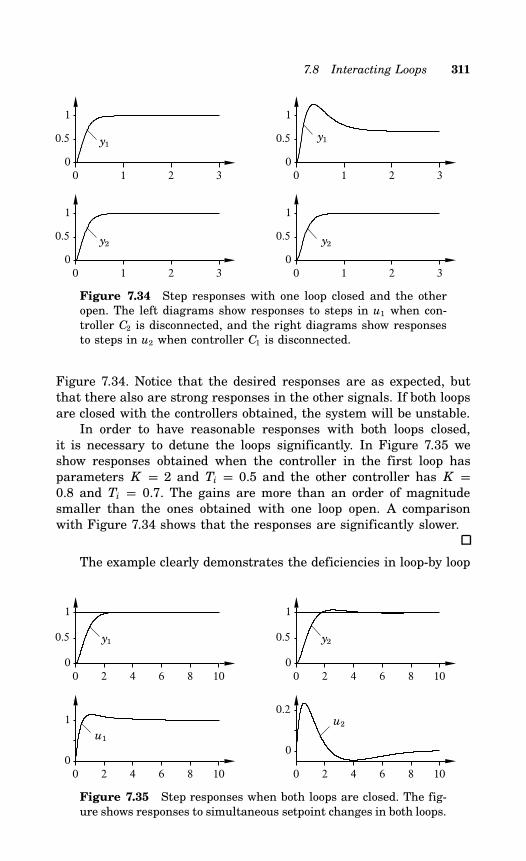
7.8 Interacting Loops 311
0 1 2 30
0.5
1
0 1 2 30
0.5
1
0 1 2 30
0.5
1
0 1 2 30
0.5
1
y1
y2
y1
y2
Figure 7.34 Step responses with one loop closed and the otheropen. The left diagrams show responses to steps in u1 when con-troller C2 is disconnected, and the right diagrams show responsesto steps in u2 when controller C1 is disconnected.
Figure 7.34. Notice that the desired responses are as expected, butthat there also are strong responses in the other signals. If both loopsare closed with the controllers obtained, the system will be unstable.In order to have reasonable responses with both loops closed,
it is necessary to detune the loops significantly. In Figure 7.35 weshow responses obtained when the controller in the first loop hasparameters K = 2 and Ti = 0.5 and the other controller has K =0.8 and Ti = 0.7. The gains are more than an order of magnitudesmaller than the ones obtained with one loop open. A comparisonwith Figure 7.34 shows that the responses are significantly slower.
The example clearly demonstrates the deficiencies in loop-by loop
0 2 4 6 8 100
0.5
1
0 2 4 6 8 100
1
0 2 4 6 8 100
0.5
1
0 2 4 6 8 10
0
0.2
y1
u1
y2
u2
Figure 7.35 Step responses when both loops are closed. The fig-ure shows responses to simultaneous setpoint changes in both loops.
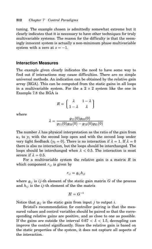
312 Chapter 7 Control Paradigms
tuning. The example chosen is admittedly somewhat extreme but itclearly indicates that it is necessary to have other techniques for trulymultivariable systems. The reason for the difficulty is that the seem-ingly innocent system is actually a non-minimum phase multivariablesystem with a zero at s = −1.
Interaction Measures
The example given clearly indicates the need to have some way tofind out if interactions may cause difficulties. There are no simpleuniversal methods. An indication can be obtained by the relative gainarray (RGA). This can be computed from the static gains in all loopsin a multivariable system. For the a 2 2 system like the one inExample 7.8 the RGA is
R = λ 1− λ
1− λ λ
where
λ = 11(0)22(0)11(0)22(0) − 12(0)21(0)
The number λ has physical interpretation as the ratio of the gain fromu1 to y1 with the second loop open and with the second loop undervery tight feedback (y2 = 0). There is no interaction if λ = 1. If λ = 0there is also no interaction, but the loops should be interchanged. Theloops should be interchanged when λ < 0.5. The interaction is mostsevere if λ = 0.5.For a multivariable system the relative gain is a matrix R in
which component ri j is given by
ri j = i jhjiwhere i j is i j-th element of the static gain matrix G of the processand hij is the i j-th element of the the matrix
H = G−1
Notice that i j is the static gain from input j to output i.Bristol’s recommendation for controller pairing is that the mea-
sured values and control variables should be paired so that the corre-sponding relative gains are positive, and as close to one as possible.If the gains are outside the interval 0.67 < λ < 1.5, decoupling canimprove the control significantly. Since the relative gain is based onthe static properties of the system, it does not capture all aspects ofthe interaction.
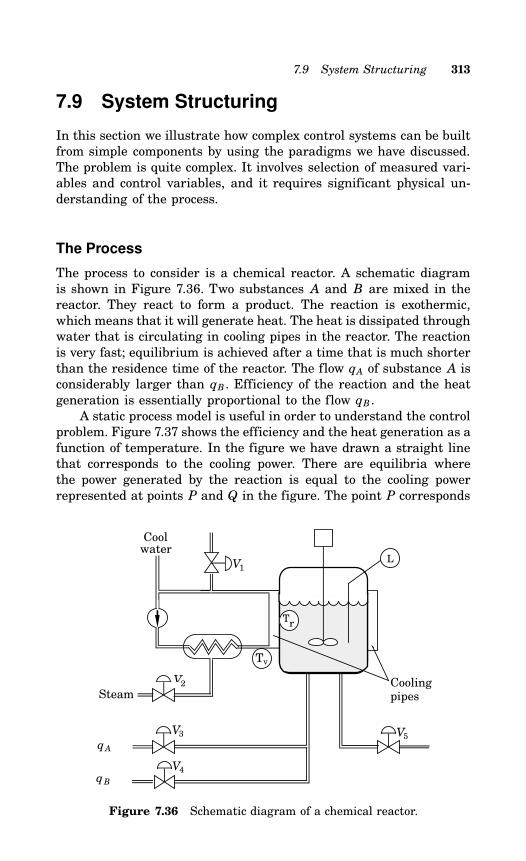
7.9 System Structuring 313
7.9 System Structuring
In this section we illustrate how complex control systems can be builtfrom simple components by using the paradigms we have discussed.The problem is quite complex. It involves selection of measured vari-ables and control variables, and it requires significant physical un-derstanding of the process.
The Process
The process to consider is a chemical reactor. A schematic diagramis shown in Figure 7.36. Two substances A and B are mixed in thereactor. They react to form a product. The reaction is exothermic,which means that it will generate heat. The heat is dissipated throughwater that is circulating in cooling pipes in the reactor. The reactionis very fast; equilibrium is achieved after a time that is much shorterthan the residence time of the reactor. The flow qA of substance A isconsiderably larger than qB . Efficiency of the reaction and the heatgeneration is essentially proportional to the flow qB .A static process model is useful in order to understand the control
problem. Figure 7.37 shows the efficiency and the heat generation as afunction of temperature. In the figure we have drawn a straight linethat corresponds to the cooling power. There are equilibria wherethe power generated by the reaction is equal to the cooling powerrepresented at points P and Q in the figure. The point P corresponds
L
Coolingpipes
Tv
qA
qB
V3
V4
V5
Tr
Steam
waterCool
V1
V2
Figure 7.36 Schematic diagram of a chemical reactor.
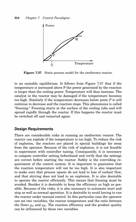
314 Chapter 7 Control Paradigms
Power
TemperatureTc
P
Q
Figure 7.37 Static process model for the exothermic reactor.
to an unstable equilibrium. It follows from Figure 7.37 that if thetemperature is increased above P the power generated by the reactionis larger than the cooling power. Temperature will thus increase. Thecatalyst in the reactor may be damaged if the temperature becomestoo high. Similarly if the temperature decreases below point P it willcontinue to decrease and the reaction stops. This phenomena is called“freezing.” Freezing starts at the surface of the cooling tube and willspread rapidly through the reactor. If this happens the reactor mustbe switched off and restarted again.
Design Requirements
There are considerable risks in running an exothermic reactor. Thereactor can explode if the temperature is too high. To reduce the riskof explosion, the reactors are placed in special buildings far awayfrom the operator. Because of the risk of explosion, it is not feasibleto experiment with controller tuning. Consequently, it is necessaryto compute controller setting beforehand and verify that the settingsare correct before starting the reactor. Safety is the overriding re-quirement of the control system. It is important to guarantee thatthe reaction temperature will not be too high. It is also importantto make sure that process upsets do not lead to loss of coolant flow,and that stirring does not lead to an explosion. It is also desirableto operate the reactor efficiently. This means that freezing must beavoided. Besides it is desirable to keep the efficiency as high as pos-sible. Because of the risks, it is also necessary to automate start andstop as well as normal operation. It is desirable to avoid having to runthe reactor under manual control. In this particular case the operatorcan set two variables, the reactor temperature and the ratio betweenthe flows qA and qB . The reaction efficiency and the product qualitycan be influenced by these two variables.
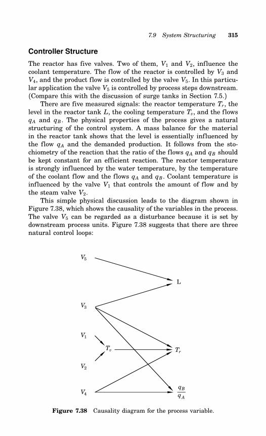
7.9 System Structuring 315
Controller Structure
The reactor has five valves. Two of them, V1 and V2, influence thecoolant temperature. The flow of the reactor is controlled by V3 andV4, and the product flow is controlled by the valve V5. In this particu-lar application the valve V5 is controlled by process steps downstream.(Compare this with the discussion of surge tanks in Section 7.5.)There are five measured signals: the reactor temperature Tr, the
level in the reactor tank L, the cooling temperature Tv, and the flowsqA and qB . The physical properties of the process gives a naturalstructuring of the control system. A mass balance for the materialin the reactor tank shows that the level is essentially influenced bythe flow qA and the demanded production. It follows from the sto-chiometry of the reaction that the ratio of the flows qA and qB shouldbe kept constant for an efficient reaction. The reactor temperatureis strongly influenced by the water temperature, by the temperatureof the coolant flow and the flows qA and qB . Coolant temperature isinfluenced by the valve V1 that controls the amount of flow and bythe steam valve V2.This simple physical discussion leads to the diagram shown in
Figure 7.38, which shows the causality of the variables in the process.The valve V5 can be regarded as a disturbance because it is set bydownstream process units. Figure 7.38 suggests that there are threenatural control loops:
Tv Tr
L
V5
V3
V1
V2
V4
qB
qA
Figure 7.38 Causality diagram for the process variable.
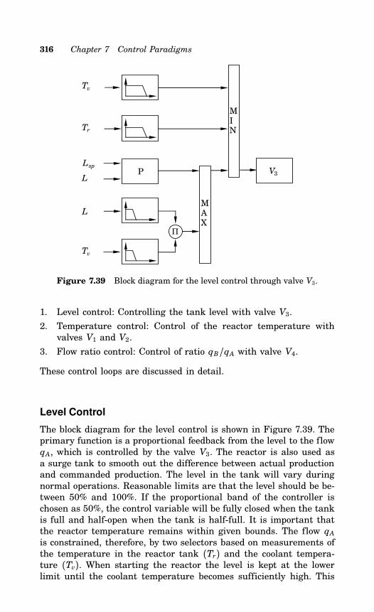
316 Chapter 7 Control Paradigms
Π
MAX
MIN
P
Tv
Tr
Tv
L
L V3
Lsp
Figure 7.39 Block diagram for the level control through valve V3.
1. Level control: Controlling the tank level with valve V3.
2. Temperature control: Control of the reactor temperature withvalves V1 and V2.
3. Flow ratio control: Control of ratio qB/qA with valve V4.These control loops are discussed in detail.
Level Control
The block diagram for the level control is shown in Figure 7.39. Theprimary function is a proportional feedback from the level to the flowqA, which is controlled by the valve V3. The reactor is also used asa surge tank to smooth out the difference between actual productionand commanded production. The level in the tank will vary duringnormal operations. Reasonable limits are that the level should be be-tween 50% and 100%. If the proportional band of the controller ischosen as 50%, the control variable will be fully closed when the tankis full and half-open when the tank is half-full. It is important thatthe reactor temperature remains within given bounds. The flow qAis constrained, therefore, by two selectors based on measurements ofthe temperature in the reactor tank (Tr) and the coolant tempera-ture (Tv). When starting the reactor the level is kept at the lowerlimit until the coolant temperature becomes sufficiently high. This
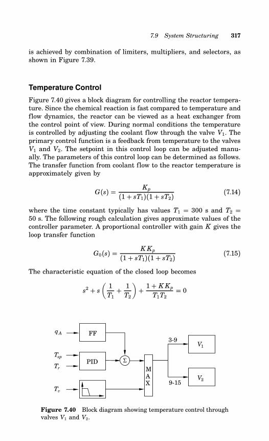
7.9 System Structuring 317
is achieved by combination of limiters, multipliers, and selectors, asshown in Figure 7.39.
Temperature Control
Figure 7.40 gives a block diagram for controlling the reactor tempera-ture. Since the chemical reaction is fast compared to temperature andflow dynamics, the reactor can be viewed as a heat exchanger fromthe control point of view. During normal conditions the temperatureis controlled by adjusting the coolant flow through the valve V1. Theprimary control function is a feedback from temperature to the valvesV1 and V2. The setpoint in this control loop can be adjusted manu-ally. The parameters of this control loop can be determined as follows.The transfer function from coolant flow to the reactor temperature isapproximately given by
G(s) = Kp
(1+ sT1)(1+ sT2) (7.14)
where the time constant typically has values T1 = 300 s and T2 =50 s. The following rough calculation gives approximate values of thecontroller parameter. A proportional controller with gain K gives theloop transfer function
G0(s) = K Kp
(1+ sT1)(1+ sT2) (7.15)
The characteristic equation of the closed loop becomes
s2 + s(1T1+ 1T2
)+ 1+ K Kp
T1T2= 0
MAX
3-9
9-15
Σ
FF
PID
V2
V1
Tv
qA
Tr
Tsp
Figure 7.40 Block diagram showing temperature control throughvalves V1 and V2.
318 Chapter 7 Control Paradigms
The closed system is thus of second order. The relative damping ζand the the undamped natural frequency ω are given by
2ζ ω = 1T1+ 1T2 1T2
(7.16)
and
2ζ ω 2 = 1+ K KpT1T2
(7.17)
The approximation in the first expression is motivated by T1 ≫ T2.With a relative damping ζ = 0.5 the Equation (7.16) then givesω 1/T2. Furthermore it follows from Equation (7.17) that
1+ K Kp = T1T2= 30050= 6
The loop gain is thus essentially determined by the ratio of the timeconstants. The controller gain becomes
K = 5Kp
and the closed-loop system has the undamped natural frequency.
ω = 1/T2 = 0.02 rad/sIf PI control is chosen instead, it is reasonable to choose a value ofthe integration time.
T1 5T2Control can be improved by using derivative action. The achievableimprovement depends on the time constant of the temperature sensor.In typical cases this time constant is between 10 s and 40 s. If it isas low as 10 s it is indeed possible to obtain improved control byintroducing a derivative action in the controller. The derivative timecan be chosen to eliminate the time constant T2. We then obtain asystem with the time constants 300 s and 10 s. The gain can then beincreased so that
1+ K Kp = 30010 = 30and the undamped natural frequency of the system then becomesω 0.1 rad/s. If the time constant of the temperature sensor isaround 40 s, the derivative action gives only marginal improvements.The heat generated by the chemical reaction is proportional to
the flow qA. To make sure that variations in qA are compensatedrapidly we have also introduced a feedforward from the flow qA. Thisfeedforward will only operate when the tank level is larger than 50%in order to avoid freezing when the reactor is started.To start the reaction the reactor must be heated so that the
temperature in the reaction vessel is larger than Tc (compare with
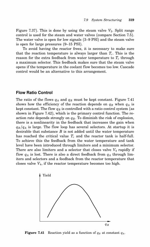
7.9 System Structuring 319
Figure 7.37). This is done by using the steam valve V2. Split rangecontrol is used for the steam and water valves (compare Section 7.5).The water valve is open for low signals (3–9 PSI) and the steam valveis open for large pressures (9–15 PSI).To avoid having the reactor freez, it is necessary to make sure
that the reaction temperature is always larger than Tc. This is thereason for the extra feedback from water temperature to Tv througha maximum selector. This feedback makes sure that the steam valveopens if the temperature in the coolant flow becomes too low. Cascadecontrol would be an alternative to this arrangement.
Flow Ratio Control
The ratio of the flows qA and qB must be kept constant. Figure 7.41shows how the efficiency of the reaction depends on qB when qA iskept constant. The flow qB is controlled with a ratio control system (asshown in Figure 7.42), which is the primary control function. The re-action rate depends strongly on qB. To diminish the risk of explosion,there is a nonlinearity in the feedback that increases the gain whenqB/qA is large. The flow loop has several selectors. At startup it isdesirable that substance B is not added until the water temperaturehas reached the critical value Tc and the reactor tank is half-full.To achieve this the feedback from the water temperature and tanklevel have been introduced through limiters and a minimum selector.There are also limiters and a selector that closes valve V4 rapidly ifflow qA is lost. There is also a direct feedback from qA through lim-iters and selectors and a feedback from the reactor temperature thatcloses valve V4, if the reactor temperature becomes too high.
qB
Yield
Figure 7.41 Reaction yield as a function of qB at constant qA.
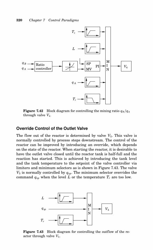
320 Chapter 7 Control Paradigms
MIN
Tv
Tr
L
qB
q A
q A
PIRatiocontroller
SPV4
MV
Figure 7.42 Block diagram for controlling the mixing ratio qB/qAthrough valve V4.
Override Control of the Outlet Valve
The flow out of the reactor is determined by valve V5. This valve isnormally controlled by process steps downstream. The control of thereactor can be improved by introducing an override, which dependson the state of the reactor. When starting the reactor, it is desirable tohave the outlet valve closed until the reactor tank is half-full and thereaction has started. This is achieved by introducing the tank leveland the tank temperature to the setpoint of the valve controller vialimiters and minimum selectors as is shown in Figure 7.43. The valveV5 is normally controlled by qsp. The minimum selector overrides thecommand qsp when the level L or the temperature Tr are too low.
MIN
Tr
L
qsp V5
Figure 7.43 Block diagram for controlling the outflow of the re-actor through valve V5.
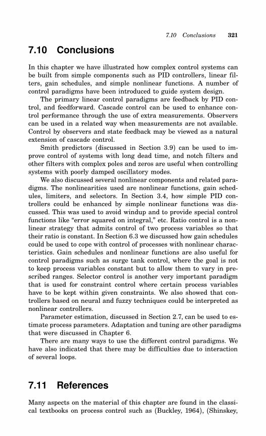
7.10 Conclusions 321
7.10 Conclusions
In this chapter we have illustrated how complex control systems canbe built from simple components such as PID controllers, linear fil-ters, gain schedules, and simple nonlinear functions. A number ofcontrol paradigms have been introduced to guide system design.The primary linear control paradigms are feedback by PID con-
trol, and feedforward. Cascade control can be used to enhance con-trol performance through the use of extra measurements. Observerscan be used in a related way when measurements are not available.Control by observers and state feedback may be viewed as a naturalextension of cascade control.Smith predictors (discussed in Section 3.9) can be used to im-
prove control of systems with long dead time, and notch filters andother filters with complex poles and zeros are useful when controllingsystems with poorly damped oscillatory modes.We also discussed several nonlinear components and related para-
digms. The nonlinearities used are nonlinear functions, gain sched-ules, limiters, and selectors. In Section 3.4, how simple PID con-trollers could be enhanced by simple nonlinear functions was dis-cussed. This was used to avoid windup and to provide special controlfunctions like “error squared on integral,” etc. Ratio control is a non-linear strategy that admits control of two process variables so thattheir ratio is constant. In Section 6.3 we discussed how gain schedulescould be used to cope with control of processes with nonlinear charac-teristics. Gain schedules and nonlinear functions are also useful forcontrol paradigms such as surge tank control, where the goal is notto keep process variables constant but to allow them to vary in pre-scribed ranges. Selector control is another very important paradigmthat is used for constraint control where certain process variableshave to be kept within given constraints. We also showed that con-trollers based on neural and fuzzy techniques could be interpreted asnonlinear controllers.Parameter estimation, discussed in Section 2.7, can be used to es-
timate process parameters. Adaptation and tuning are other paradigmsthat were discussed in Chapter 6.There are many ways to use the different control paradigms. We
have also indicated that there may be difficulties due to interactionof several loops.
7.11 References
Many aspects on the material of this chapter are found in the classi-cal textbooks on process control such as (Buckley, 1964), (Shinskey,
322 Chapter 7 Control Paradigms
1988), and (Seborg et al., 1989). A more specialized presentation isgiven in (Hägglund, 1991). The books (Shinskey, 1981) and (Klefenz,1986) focus on applications to energy systems.The methods discussed in this chapter can all be characterized as
bottom-up procedures in the sense that a complex system is built upby combining simple components. An interesting view of this is pre-sented in (Bristol, 1980). A top-down approach is another possibility.A discussion of this, which is outside the scope of this book, is foundin (Seborg et al., 1986).Cascade and feedforward control are treated in the standard texts
on control. A presentation with many practical aspects is found in(Tucker and Wills, 1960). Selector control is widely used in practice.A general presentation is given in (Åström, 1987b). Many applicationsare given in the books (Shinskey, 1978) and (Klefenz, 1986). Analysisof a simple scheme is given in (Foss, 1981). It is difficult to analysenonlinear systems. A stability analysis of a system with selectors isgiven in (Foss, 1981).Fuzzy control has been around for a long time, see (Mamdani,
1974), (Mamdani and Assilian, 1974), (King and Mamdani, 1977),and (Tong, 1977). It has recently received a lot of attention particu-larly in Japan: see (Zadeh, 1988), (Tong, 1984), (Sugeno, 1985), (Dri-ankov et al., 1993), and (Wang, 1994). The technique has been usedfor automation of complicated processes that have previously beencontrolled manually. Control of cement kilns is a typical example, see(Holmblad and stergaard, 1981). There has been a similar devel-opment in neural networks, see, for example, (Hecht-Nielsen, 1990),(Pao, 1990), and (Åström and McAvoy, 1992). There was a lot of activ-ity in neural networks during the late 1960s, which vanished rapidly.There was a rapid resurgence of interest in the 1980s. There are alot of exaggerations both in fuzzy and neural techniques, and no bal-anced view of the relevance of the fields for control has yet emerged.The paper (Willis et al., 1991) gives an overview of possible uses ofneural networks for process control, and the paper (Pottman and Se-borg, 1993) describes an application to control of pH. The papers (Lee,1990), (Huang, 1991), and (Swiniarski, 1991) describe applications toPID controllers and their tuning. There have also been attempts tomerge fuzzy and neural control, see (Passino and Antsaklis, 1992)and (Brown and Harris, 1994).Some fundamental issues related to interaction in systems are
treated in (Rijnsdorp, 1965a), (Rijnsdorp, 1965b), and (McAvoy, 1983).The relative gain array was described in (Bristol, 1966). Control ofsystems with strong interaction between many loops require tech-niques that are very different from those discussed in this chapter,see, for example, (Cutler and Ramaker, 1980) and (Seborg et al.,1986). Section 7.9 is based on (Buckley, 1970).
INDEX
Index Terms Links
Ms-value 125
λ-tuning 156 198
A
ABB 258
Accutune 250
adaptive control 233
adaptive feedforward 249
adaptive techniques 232
adaptive techniques, adaptive
control 233
adaptive techniques, adaptive
feedforward 249
adaptive techniques, automatic
tuning 230 234
adaptive techniques, gain
scheduling 232 234
adaptive techniques, uses of 236
air-fuel ratio control 291 294
Alfa Laval Automation 247
aliasing 94
amplitude margin 125 126
analytical tuning 156
This page has been reformatted by Knovel to provide easier navigation.
Index Terms Links
anti-windup 80
antialiasing filter 94
anticipating action 117
apparent dead time 16
apparent time constant 16
approximate models 51
area methods 24
auto-tuning 233 234
automatic reset 67 117
automatic tuning 230 234
average residence time 13 27
averaging control 132
B
back propagation 298
back-calculation 83
backlash 264
batch unit 91
BO, modulus optimum 166 198
bumpless transfer 103 105
Butterworth filter 94
C
cancellation of process poles 163 169
cascade control 274
cascade control, applications 279
cascade control, control
modes 277
This page has been reformatted by Knovel to provide easier navigation.
Index Terms Links
cascade control, disturbance
rejection 275
cascade control, tuning 278
cascade control, use of 276
cascade control, windup 278
centrifugal governor 117
Chien, Hrones and Reswick
method 149
CHR method 149
Cohen-Coon method 180
commercial controllers 108
conditional integration 88
control error 60
control paradigms 273
control signal overshoot 129
control variable 5
controllability ratio 16
controller design 120
controller gain K 61 64
controller outputs 77
crisp variable 298
cut-back 89
D
D-term 64
Dahlin method 198
DCS Tuner 258
dead time 13
This page has been reformatted by Knovel to provide easier navigation.
Index Terms Links
dead time, λ-tuning 156
dead time, apparent 16
dead time, compensation 112
dead time, normalized 16
dead time, PPI controller 157
dead time, Smith predictor 113
decay ratio 127
defuzzification 301
derivative action 69 117
derivative gain limitation 76
derivative time Td 64
describing function 38
diagnosis 262
digital signal processors 118
direct adaptive control 233
disturbance models 46
disturbance rejection 193
disturbance representation 50
disturbances 53
dominant pole design 179
dominant poles 132
drum level control 283
dynamic model 8
E
ECA400 247
error feedback 73
error-squared controllers 77
This page has been reformatted by Knovel to provide easier navigation.
Index Terms Links
EXACT 244
F
feedback 60 273
feedforward control 281
feedforward control, adaptive 249
feedforward control, dynamic 282
feedforward control, static 282
feedforward control, tuning 287
Fisher-Rosemount 254
four-parameter model 19
Foxboro 244
frequence curve 10
frequency response 9 34
friction 262
fuzzy control 298
fuzzy inference 300
fuzzy logic 298
G
gain margin 126
gain ratio k 36
gain scheduling 232 234
H
Haalmans method 159
Honeywell 250 257
This page has been reformatted by Knovel to provide easier navigation.
Index Terms Links
hysteresis 264
I
I-PD controller 74
I-term 64
IAE 122
IE 122
IMC, internal model control 162
impulse 47
impulse response 9 21
incremental algorithm 79
incremental algorithm,
discretization 99
incremental algorithm,
windup 82
indirect adaptive control 233
integral action 67 117
integral time Ti 64
integral windup, SEE
WINDUP 80
integrated absolute error,
IAE 122
integrated error, IE 122
integrated squared error,
ISE 124
integrator clamping 88
integrator windup, SEE
This page has been reformatted by Knovel to provide easier navigation.
Index Terms Links
integrator windup, SEE (Cont.)
WINDUP 80
interacting loops 304
interaction 309
interaction measures 312
internal model control,
IMC 162
ISE 124
ISTE 128
ITAE 128
ITE 128
ITSE 128
J
jump- and rate limiter 288
K
Kappa-Tau tuning 202
KT tuning 202
KT tuning, examples 224
KT tuning, frequency response
methods 212
KT tuning, performance
assessment 220
KT tuning, step response
methods 203
This page has been reformatted by Knovel to provide easier navigation.
Index Terms Links
L
lambda tuning 156 198
Laplace transform 11
least squares 44
least squares, recursive 45
limiters 287
linear time-invariant system 8
load disturbances 54
load disturbances,
specifications 121
loop gain 65
loop shaping 151
Looptune 257
M
manipulated variable 5
maximum selector 292
measurement noise 54 121
median selector 295
methods of moments 24
minimum selector 292
mode switches 103
model approximation 55
model following 284
model uncertainty 121
This page has been reformatted by Knovel to provide easier navigation.
Index Terms Links
model-based tuning 237
modulus optimum, BO 166
N
negative feedback 5 60
neural network 295
neural network, hidden
layers 297
neural network, learning 297
neuron 296
noise 47
non-minimum phase 13
nonlinear elements 287
nonlinearities 52
normalized dead time τ 16
notch filter 113
Nyquist curve 10
O
observers 280
on-off control 60
operational aspects 103
optimization methods 164
oscillatory systems 23
overshoot 127
overshoot, control signal 129
This page has been reformatted by Knovel to provide easier navigation.
Index Terms Links
P
P-term 64
pairing 309
parallel systems 305
parameter estimation 43 241
parametric models 43
phase margin 126
PI-D controller 74
PID control 59 64
PID, classical form 73
PID, digital implementation 93
PID, discretization 95
PID, ideal form 73
PID, interacting form 71
PID, ISA form 73
PID, non-interacting form 71
PID, parallel form 73
PID, series form 73
PID, standard form 73
pole placement 173
pole-zero cancellation 160 261
PPI controller 157
pre-act 117
predictive PI controller 157
prefiltering 94
preload 89
process gain 13
This page has been reformatted by Knovel to provide easier navigation.
Index Terms Links
process models 5
process noise 7
process variable, PV 5
process variations 53
proportional action 64 117
proportional band 61 87
proportional control 61
proportional control, static
analysis 62
Protuner 259
ProvoxTM 254
pulse transfer function 43
pulse width modulation 78
PV, process variable 5
Q
quantization 100
R
ramp 47
ramp unit 288
rate limiter 288
ratio control 290
ratio control, for air-fuel 291
ratio controllers 290
ratio PI controller 290
reaction curve 9
This page has been reformatted by Knovel to provide easier navigation.
Index Terms Links
reference variable, SEE
SETPOINT 5
relative damping 130
relative gain array 312
relay auto-tuning 239
relay feedback 37
relay with hysteresis 39
reset 64 67
residence time approximation 14
response curve 58
RGA, relative gain array 312
rise time 127
robustness 164
Rosenbrock’s system, 310
RPI controller 290
RS3TM 254
rule-based methods 241
S
sampling 93
selector control 292
selector control, applications 294
selector control, of air-fuel 294
selector control, tuning 294
sensitivity 124
sensitivity function 124 125 158
sensitivity, maximum Ms 125
This page has been reformatted by Knovel to provide easier navigation.
Index Terms Links
sensitivity, to measurement
noise 124
sensitivity, to process
characteristics 124
series form 91
setpoint limitation 82
setpoint, following 53
setpoint, SP 5
setpoint, specifications 121 126
setpoint, weighting 73 192
settling time 127
sinusoid 47
SLPC-181 281 253
Smith predictor 113
SO, symmetrical optimum 166 198
SP, setpoint 5
specifications 121
spectral density 48
split range control 291 319
state feedback 281
static analysis 62
static model 6
static process characteristic 6 62
steady-state error 64 66 127
step 47
step response 9
step response models 11
step response, integrating 12
This page has been reformatted by Knovel to provide easier navigation.
Index Terms Links
step response, monotone 12
step response, oscillating 12
step response, parametric
models 53
stick-slip motion 262
stiction 262
superposition principle 8
surge tank control 289
symmetrical optimum, SO 166
system structuring 313
T
Techmation 259
three-parameter model 15 28 32
three-position pulse output 101
thyristors 77
tracking 83 105
tracking time constant 85 88
transfer function 11
transient response 8 11
triacs 77
tuning maps 146
two-degree-of-freedom controller 74 285
two-parameter model 13
U
UDC 6000 250
ultimate frequency 10
This page has been reformatted by Knovel to provide easier navigation.
Index Terms Links
ultimate gain 36
ultimate point 10
undamped natural frequency 130
unmodeled dynamics 51
V
velocity algorithms 79 99
W
weighted moments 32
windup 80
windup, back-calculation 83
windup, cascade control 278
windup, conditional integration 88
windup, incremental algorithm 82
windup, selector control 294
windup, setpoint limitation 82
windup, tracking 83
word length 100
Y
Yokogawa 253
Z
Ziegler-Nichols methods 134
Ziegler-Nichols, frequency
response method 34 136
This page has been reformatted by Knovel to provide easier navigation.

Index Terms Links
Ziegler-Nichols, modified 140
Ziegler-Nichols, properties 142
Ziegler-Nichols, relations 138
Ziegler-Nichols, step response
method 135
This page has been reformatted by Knovel to provide easier navigation.
Bibliography
Anderson, K. L., G. L. Blankenship, and L. G. Lebow (1988): “A rule-based PID controller.” In Proc. IEEE Conference on Decision andControl, Austin, Texas.
Anderssen, A. S. and E. T. White (1970): “Parameter estimation bythe transfer function method.” Chemical Engineering Science, 25,pp. 1015–1021.
Anderssen, A. S. and E. T. White (1971): “Parameter estimation bythe weighted moments method.” Chemical Engineering Science,26, pp. 1203–1221.
Antsaklis, P. J., K. M. Passino, and S. J. Wang (1991): “An intro-duction to autonomous control systems.” IEEE Control SystemsMagazine, 11:4, pp. 5–13.
Åström, K. J. (1987a): “Adaptive feedback control.” Proc. IEEE, 75,February, pp. 185–217. Invited paper.
Åström, K. J. (1987b): “Advanced control methods—Survey and as-sessment of possibilities.” In Morris and Williams, Eds., Ad-vanced Control in Computer Integrated Manufacturing, Proceed-ings 13th Annual Advanced Control Conference. Purdue Univer-sity, West Lafayette, Indiana.
Åström, K. J. (1991): “Assessment of achievable performance of simplefeedback loops.” International Journal of Adaptive Control andSignal Processing, 5, pp. 3–19.
Åström, K. J. (1992): “Autonomous control.” In Bensoussan and Ver-jus, Eds., Future Tendencies in Computer Science, Control andApplied Mathematics, volume 653 of Lecture Notes in ComputerScience, pp. 267–278. Springer-Verlag.
Åström, K. J. and T. Hägglund (1984): “Automatic tuning of simpleregulators with specifications on phase and amplitude margins.”Automatica, 20, pp. 645–651.
Åström, K. J. and T. Hägglund (1988): Automatic Tuning of PIDControllers. Instrument Society of America, Research TrianglePark, North Carolina.
323
324 Bibliography
Åström, K. J., T. Hägglund, C. C. Hang, and W. K. Ho (1993): “Au-tomatic tuning and adaptation for PID controllers—A survey.”Control Engineering Practice, 1:4, pp. 699–714.
Åström, K. J., C. C. Hang, P. Persson, and W. K. Ho (1992): “Towardsintelligent PID control.” Automatica, 28:1, pp. 1–9.
Åström, K. J. and T. J. McAvoy (1992): “Intelligent control.” Journalof Process Control, 2:2, pp. 1–13.
Åström, K. J. and L. Rundqwist (1989): “Integrator windup and howto avoid it.” In Proceedings of the American Control Conference(ACC ’89), pp. 1693–1698, Pittsburgh, Pennsylvania.
Åström, K. J. and H. Steingrímsson (1991): “Implementation of a PIDcontroller on a DSP.” In Ahmed, Ed., Digital Control Applicationswith the TMS 320 Family, Selected Application Notes, pp. 205–238. Texas Instruments.
Åström, K. J. and B. Wittenmark (1984): Computer ControlledSystems—Theory and Design. Prentice-Hall, Englewood Cliffs,New Jersey.
Åström, K. J. and B. Wittenmark (1989): Adaptive Control. Addison-Wesley, Reading, Massachusetts.
Åström, K. J. and B. Wittenmark (1990): Computer Controlled Sys-tems—Theory and Design. Prentice-Hall, Englewood Cliffs, NewJersey, second edition.
Atherton, D. P. (1975): Nonlinear Control Engineering—DescribingFunction Analysis and Design. Van Nostrand Reinhold Co., Lon-don, UK.
Bialkowski, W. L. (1993): “Dreams versus reality: A view from bothsides of the gap.” Pulp and Paper Canada, 94:11.
Blickley, G. (1990): “Modern control started with ziegler-nichols tun-ing.” Control Engineering, October, pp. 11–17.
Blickley, G. J. (1988): “PID tuning made easy with hand-held com-puter.” Control Engineering, November, p. 99.
Boyd, S. P. and C. H. Barratt (1991): Linear Controller Design – Limitsof Performance. Prentice Hall Inc., Englewood Cliffs, New Jersey.
Bristol, E. (1966): “On a new measure of interaction for multivariableprocess control.” IEEE Transactions on Automatic Control, 11,p. 133.
Bristol, E. H. (1967): “A simple adaptive system for industrial control.”Instrumentation Technology, June.
Bristol, E. H. (1970): “Adaptive control odyssey.” In ISA Silver JubileeConference, Paper 561–570, Philadelphia.
Bristol, E. H. (1977): “Pattern recognition: An alternative to param-
Bibliography 325
eter identification in adaptive control.” Automatica, 13, pp. 197–202.
Bristol, E. H. (1980): “After DDC: Idiomatic (structured) control.”In Proceedings American Institute of Chemical Engineering(AIChE), Philadelphia.
Bristol, E. H. (1986): “The EXACT pattern recognition adaptive con-troller, a user-oriented commercial success.” In Narendra, Ed.,Adaptive and Learning Systems, pp. 149–163, New York. PlenumPress.
Bristol, E. H., G. R. Inaloglu, and J. F. Steadman (1970): “Adaptiveprocess control by pattern recognition.” Instrum. Control Systems,pp. 101–105.
Bristol, E. H. and T. W. Kraus (1984): “Life with pattern adaptation.”In Proc. 1984 American Control Conference, San Diego, Califor-nia.
Brown, M. and C. Harris (1994): Neurofuzzy Adaptive Modelling andControl. Prentice Hall.
Buckley, P. S. (1964): Techniques of Process Control. John Wiley &Sons, Inc.
Buckley, P. S. (1970): “Protective controls for a chemical reactor.”Chemical Engineering, April, pp. 145–150.
Callaghan, P. J., P. L. Lee, and R. B. Newell (1986): “Evaluation offoxboro controller.” Process Control Engineering, May, pp. 38–40.
Callender, A., D. R. Hartree, and A. Porter (1936): “Time lag in acontrol system.” Philos. Trans. A., 235, pp. 415–444.
Cameron, F. and D. E. Seborg (1983): “A self-tuning controller witha PID structure.” Int. J. Control, 38:2, pp. 401–417.
Chen, B.-S. and S.-S. Wang (1988): “The stability of feedback con-trol with nonlinear saturating actuator: Time domain approach.”IEEE Transactions on Automatic Control, 33, pp. 483–487.
Chen, C.-L. (1989): “A simple method for on-line identification andcontroller tuning.” AIChE Journal, 35:12, pp. 2037–2039.
Chien, I. L. (1988): “IMC-PID controller design—an extension.”In IFAC Symposium, Adaptive Control of Chemical Processes,pp. 155–160, Copenhagen, Denmark.
Chien, I.-L. and P. S. Fruehauf (1990): “Consider IMC tuning toimprove controller performance.” Chemical Engineering Progress,October, pp. 33–41.
Chien, K. L., J. A. Hrones, and J. B. Reswick (1952): “On the auto-matic control of generalized passive systems.” Trans. ASME, 74,pp. 175–185.
326 Bibliography
Clarke, D. W. (1984): “PID algorithms and their computer implemen-tation.” Trans. Inst. M. C., 6:6, pp. 305–316.
Close, C. M. and D. K. Frederick (1993): Modeling and Analysis ofDynamic Systems. Houghton Mifflin.
Cohen, G. H. and G. A. Coon (1953): “Theoretical consideration ofretarded control.” Trans. ASME, 75, pp. 827–834.
Coon, G. A. (1956a): “How to find controller settings from processcharacteristics.” Control Engineering, 3, pp. 66–76.
Coon, G. A. (1956b): “How to set three-term controller.” Control En-gineering, 3, pp. 71–76.
Corripio, A. B. (1990): Tuning of Industrial Control Systems. Instru-ment Society of America.
Cutler, C. R. and B. C. Ramaker (1980): “Dynamic matrix control—A computer control algorithm.” In Proceedings Joint AutomaticControl Conference, Paper WP5-B, San Francisco, California.
Dahlin, E. B. (1968): “Designing and tuning digital controllers.” In-struments and Control Systems, 42, June, pp. 77–83.
Deshpande, P. B. and R. H. Ash (1981): Elements of Computer ProcessControl with Advanced Control Applications. Instrument Societyof America, Research Triangle Park, North Carolina.
Dreinhofer, L. H. (1988): “Controller tuning for a slow nonlinear pro-cess.” IEEE Control Systems Magazine, 8:2, pp. 56–60.
Driankov, D., H. Hellendoorn, and M. Reinfrank (1993): An Introduc-tion to Fuzzy Control. Springer-Verlag.
Dumont, G. A. (1986): “On the use of adaptive control in the pro-cess industries.” In Morari and McAvoy, Eds., Proceedings ThirdInternational Conference on Chemical Process Control–CPCIII,Amsterdam. Elsevier.
Dumont, G. A., J. M. Martin-S nchez, and C. C. Zervos (1989): “Com-parison of an auto-tuned PID regulator and an adaptive predic-tive control system on an industrial bleach plant.” Automatica,25, pp. 33–40.
Elgerd, O. I. and W. C. Stephens (1959): “Effect of closed-loop transferfunction pole and zero locations on the transient response oflinear control systems.” Applications and Industry, 42, pp. 121–127.
Ender, D. B. (1993): “Process control performance: Not as good as youthink.” Control Engineering, 40:10, pp. 180–190.
Fertik, H. A. (1975): “Tuning controllers for noisy processes.” ISATransactions, 14, pp. 292–304.
Fertik, H. A. and C. W. Ross (1967): “Direct digital control algorithms
Bibliography 327
with anti-windup feature.” ISA Trans., 6:4, pp. 317–328.
Foss, A. M. (1981): “Criterion to assess stability of a ‘lowest wins’control strategy.” IEEE Proc. Pt. D, 128:1, pp. 1–8.
Foxboro, Inc. (1979): Controller Tuning Guide, PUB 342A.Frank, P. M. (1990): “Fault diagnosis in dynamic systems using an-
alytical and knowledge-based redundancy—A survey and somenew results.” Automatica, 26:3, pp. 459–474.
Fröhr, F. (1967): “Optimierung von Regelkreisen nach dem Betrag-soptimum und dem symmetrischen Optimum.” Automatik, 12,January, pp. 9–14.
Fröhr, F. and F. Orttenburger (1982): Introduction to Electronic Con-trol Engineering. Siemens Aktiengesellschaft, Heyden & Son Ltd,London.
Gallun, S. E., C. W. Matthews, C. P. Senyard, and B. Slater (1985):“Windup protection and initialization for advanced digital con-trol.” Hydrocarbon Processing, June, pp. 63–68.
Gawthrop, P. J. (1986): “Self-tuning PID controllers: Algorithms andimplementation.” IEEE Transactions on Automatic Control, 31,pp. 201–209.
Gelb, A. and W. E. V. Velde (1968): Multiple-Input Describing Func-tions and Nonlinear System Design. McGraw-Hill, New York.
Gerry, J. P. (1987): “A comparison of PID controller algorithms.” Con-trol Engineering, March, pp. 102–105.
Gille, J. C., M. J. Pelegrin, and P. Decaulne (1959): Feedback ControlSystems. McGraw-Hill, New York.
Glattfelder, A. H., L. Guzzella, and W. Schaufelberger (1988): “Bump-less transfer, anti-reset-windup, saturating and override controls:A status report on self-tuning regulators.” In Proceedings ofIMACS-88, Part 2, pp. 66–72, Paris, France.
Glattfelder, A. H. and Schaufelberger (1983): “Stability analysis ofsingle loop systems with saturation and antireset-windup cir-cuits.” IEEE Transactions on Automatic Control, 28, pp. 1074–1081.
Glattfelder, A. H. and W. Schaufelberger (1986): “Start-up per-formance of different proportional-integral-anti-wind-up regula-tors.” International Journal of Control, 44, pp. 493–505.
Goff, K. W. (1966a): “Dynamics in direct digital control I—Estimatingcharacteristics and effects of noisy signals.” ISA Journal, 13,November, pp. 45–49.
Goff, K. W. (1966b): “Dynamics in direct digital control II—A sys-tematic approach to DDC design.” ISA Journal, 13, December,
328 Bibliography
pp. 44–54.
Graham, D. and R. C. Lathrop (1953): “The synthesis of ‘optimum’transient response: Criteria and standard forms.” Transactionsof the AIEE, 72, November, pp. 273–288.
Grebe, J. J., R. H. Boundy, and R. W. Cermak (1933): “The controlof chemical processes.” Trans. of American Institute of ChemicalEngineers, 29, pp. 211–255.
Haalman, A. (1965): “Adjusting controllers for a deadtime process.”Control Engineering, July-65, pp. 71–73.
Habel, F. (1980): “Ein Verfahren zur Bestimmung der Parameternvon PI-, PD- und PID-Reglern.” Regelungstechnik, 28:6, pp. 199–205.
Hägglund, T. (1991): Process Control in Practice. Chartwell-Bratt Ltd,Bromley, UK.
Hägglund, T. (1992): “A predictive PI controller for processes withlong dead times.” IEEE Control Systems Magazine, 12:1, pp. 57–60.
Hägglund, T. (1993): “Disturbance supervision in feedback loops.” InPreprints Tooldiag’93, International Conference on Fault Diagno-
sis, Toulouse, France.
Hägglund, T. and K. J. Åström (1991): “Industrial adaptive con-trollers based on frequency response techniques.” Automatica, 27,pp. 599–609.
Hang, C. C., K. J. Åström, and W. K. Ho (1991): “Refinements of theZiegler-Nichols tuning formula.” IEE Proceedings, Part D, 138:2,pp. 111–118.
Hang, C. C., K. J. Åström, and W. K. Ho (1993a): “Relay auto-tuningin the presence of static load disturbance.” Automatica, 29:2,pp. 563–564.
Hang, C. C., T. H. Lee, and W. K. Ho (1993b): Adaptive Control.Instrument Society of America, Research Triangle Park, NorthCarolina.
Hang, C. C. and K. K. Sin (1991): “An on-line auto-tuning methodbased on cross-correlation.” IEEE Transactions on IndustrialElectronics, 38:6, pp. 428–437.
Hanus, R. (1988): “Antiwindup and bumpless transfer: a survey.” InProceedings of IMACS-88, Part 2, pp. 59–65, Paris, France.
Hanus, R., M. Kinnaert, and J.-L. Henrotte (1987): “Conditioningtechnique, a general anti-windup and bumpless transfer method.”Automatica, 23:729–739.
Harriott, P. (1964): Process Control. McGraw-Hill, New York.
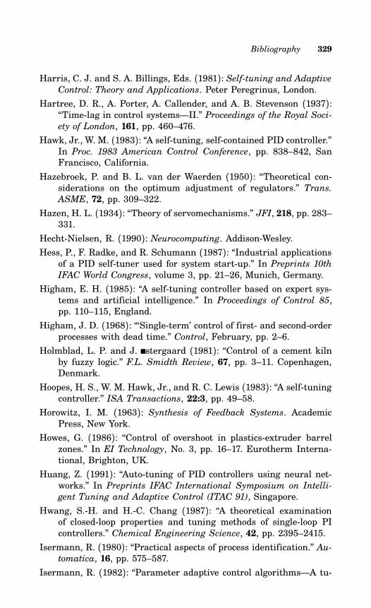
Bibliography 329
Harris, C. J. and S. A. Billings, Eds. (1981): Self-tuning and AdaptiveControl: Theory and Applications. Peter Peregrinus, London.
Hartree, D. R., A. Porter, A. Callender, and A. B. Stevenson (1937):“Time-lag in control systems—II.” Proceedings of the Royal Soci-ety of London, 161, pp. 460–476.
Hawk, Jr., W. M. (1983): “A self-tuning, self-contained PID controller.”In Proc. 1983 American Control Conference, pp. 838–842, SanFrancisco, California.
Hazebroek, P. and B. L. van der Waerden (1950): “Theoretical con-siderations on the optimum adjustment of regulators.” Trans.ASME, 72, pp. 309–322.
Hazen, H. L. (1934): “Theory of servomechanisms.” JFI, 218, pp. 283–331.
Hecht-Nielsen, R. (1990): Neurocomputing. Addison-Wesley.Hess, P., F. Radke, and R. Schumann (1987): “Industrial applications
of a PID self-tuner used for system start-up.” In Preprints 10thIFAC World Congress, volume 3, pp. 21–26, Munich, Germany.
Higham, E. H. (1985): “A self-tuning controller based on expert sys-tems and artificial intelligence.” In Proceedings of Control 85,pp. 110–115, England.
Higham, J. D. (1968): “‘Single-term’ control of first- and second-orderprocesses with dead time.” Control, February, pp. 2–6.
Holmblad, L. P. and J. stergaard (1981): “Control of a cement kilnby fuzzy logic.” F.L. Smidth Review, 67, pp. 3–11. Copenhagen,Denmark.
Hoopes, H. S., W. M. Hawk, Jr., and R. C. Lewis (1983): “A self-tuningcontroller.” ISA Transactions, 22:3, pp. 49–58.
Horowitz, I. M. (1963): Synthesis of Feedback Systems. AcademicPress, New York.
Howes, G. (1986): “Control of overshoot in plastics-extruder barrelzones.” In EI Technology, No. 3, pp. 16–17. Eurotherm Interna-tional, Brighton, UK.
Huang, Z. (1991): “Auto-tuning of PID controllers using neural net-works.” In Preprints IFAC International Symposium on Intelli-gent Tuning and Adaptive Control (ITAC 91), Singapore.
Hwang, S.-H. and H.-C. Chang (1987): “A theoretical examinationof closed-loop properties and tuning methods of single-loop PIcontrollers.” Chemical Engineering Science, 42, pp. 2395–2415.
Isermann, R. (1980): “Practical aspects of process identification.” Au-tomatica, 16, pp. 575–587.
Isermann, R. (1982): “Parameter adaptive control algorithms—A tu-
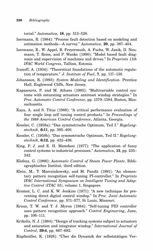
330 Bibliography
torial.” Automatica, 18, pp. 513–528.
Isermann, R. (1984): “Process fault detection based on modeling andestimation methods—A survey.” Automatica, 20, pp. 387–404.
Isermann, R., W. Appel, B. Freyermuth, A. Fuchs, W. Janik, D. Neu-mann, T. Reiss, and P. Wanke (1990): “Model based fault diag-nosis and supervision of machines and drives.” In Preprints 11thIFAC World Congress, Tallinn, Estonia.
Ivanoff, A. (1934): “Theoretical foundations of the automatic regula-tion of temperature.” J. Institute of Fuel, 7, pp. 117–138.
Johansson, R. (1993): System Modeling and Identification. PrenticeHall, Englewood Cliffs, New Jersey.
Kapasouris, P. and M. Athans (1985): “Multivariable control sys-tems with saturating actuators antireset windup strategies.” InProc. Automatic Control Conference, pp. 1579–1584, Boston, Mas-sachusetts.
Kaya, A. and S. Titus (1988): “A critical performance evaluation offour single loop self tuning control products.” In Proceedings ofthe 1988 American Control Conference, Atlanta, Georgia.
Kessler, C. (1958a): “Das symmetrische Optimum, Teil I.” Regelung-stechnik, 6:11, pp. 395–400.
Kessler, C. (1958b): “Das symmetrische Optimum, Teil II.” Regelung-stechnik, 6:12, pp. 432–436.
King, P. J. and E. H. Mamdani (1977): “The application of fuzzycontrol systems to industrial processes.” Automatica, 13, pp. 235–242.
Klefenz, G. (1986): Automatic Control of Steam Power Plants. Bibli-ographisches Institut, third edition.
Klein, M., T. Marczinkowsky, and M. Pandit (1991): “An elemen-tary pattern recognition self-tuning PI-controller.” In PreprintsIFAC International Symposium on Intelligent Tuning and Adap-
tive Control (ITAC 91), volume 1, Singapore.
Kramer, L. C. and K. W. Jenkins (1971): “A new technique for pre-venting direct digital control windup.” In Proc. Joint AutomaticControl Conference, pp. 571–577, St Louis, Missouri.
Kraus, T. W. and T. J. Myron (1984): “Self-tuning PID controlleruses pattern recognition approach.” Control Engineering, June,pp. 106–111.
Krikelis, N. J. (1984): “Design of tracking systems subject to actuatorsand saturation and integrator windup.” International Journal ofControl, 39:4, pp. 667–682.
Küpfmüller, K. (1928): “Über die Dynamik der selbststätigen Ver-
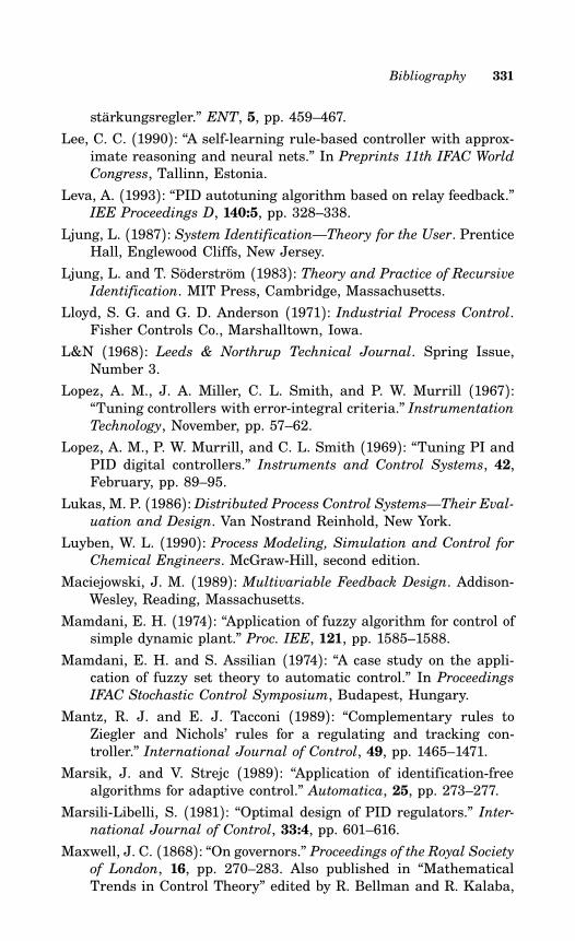
Bibliography 331
stärkungsregler.” ENT, 5, pp. 459–467.
Lee, C. C. (1990): “A self-learning rule-based controller with approx-imate reasoning and neural nets.” In Preprints 11th IFAC WorldCongress, Tallinn, Estonia.
Leva, A. (1993): “PID autotuning algorithm based on relay feedback.”IEE Proceedings D, 140:5, pp. 328–338.
Ljung, L. (1987): System Identification—Theory for the User. PrenticeHall, Englewood Cliffs, New Jersey.
Ljung, L. and T. Söderström (1983): Theory and Practice of RecursiveIdentification. MIT Press, Cambridge, Massachusetts.
Lloyd, S. G. and G. D. Anderson (1971): Industrial Process Control.Fisher Controls Co., Marshalltown, Iowa.
L&N (1968): Leeds & Northrup Technical Journal. Spring Issue,Number 3.
Lopez, A. M., J. A. Miller, C. L. Smith, and P. W. Murrill (1967):“Tuning controllers with error-integral criteria.” InstrumentationTechnology, November, pp. 57–62.
Lopez, A. M., P. W. Murrill, and C. L. Smith (1969): “Tuning PI andPID digital controllers.” Instruments and Control Systems, 42,February, pp. 89–95.
Lukas, M. P. (1986): Distributed Process Control Systems—Their Eval-uation and Design. Van Nostrand Reinhold, New York.
Luyben, W. L. (1990): Process Modeling, Simulation and Control forChemical Engineers. McGraw-Hill, second edition.
Maciejowski, J. M. (1989): Multivariable Feedback Design. Addison-Wesley, Reading, Massachusetts.
Mamdani, E. H. (1974): “Application of fuzzy algorithm for control ofsimple dynamic plant.” Proc. IEE, 121, pp. 1585–1588.
Mamdani, E. H. and S. Assilian (1974): “A case study on the appli-cation of fuzzy set theory to automatic control.” In ProceedingsIFAC Stochastic Control Symposium, Budapest, Hungary.
Mantz, R. J. and E. J. Tacconi (1989): “Complementary rules toZiegler and Nichols’ rules for a regulating and tracking con-troller.” International Journal of Control, 49, pp. 1465–1471.
Marsik, J. and V. Strejc (1989): “Application of identification-freealgorithms for adaptive control.” Automatica, 25, pp. 273–277.
Marsili-Libelli, S. (1981): “Optimal design of PID regulators.” Inter-national Journal of Control, 33:4, pp. 601–616.
Maxwell, J. C. (1868): “On governors.” Proceedings of the Royal Societyof London, 16, pp. 270–283. Also published in “MathematicalTrends in Control Theory” edited by R. Bellman and R. Kalaba,
332 Bibliography
Dover Publications, New York 1964, pp. 3–17.
McAvoy, T. J. (1983): Interaction Analysis: Principles and Applica-tions. Instrument Society of America, Research Triangle Park,North Carolina.
McMillan, G. K. (1983): Tuning and Control Loop Performance. In-strument Society of America, Research Triangle Park, North Car-olina, second edition.
McMillan, G. K. (1986): “Advanced control algorithms: Beware of falseprophecies.” InTech, January, pp. 55–57.
McMillan, G. K., W. K. Wojsznis, and G. T. Borders, Jr (1993a):“Flexible gain scheduler.” In Advances in Instrumentation andControl, volume 48 of ISA Conference, pp. 811–818.
McMillan, G. K., W. K. Wojsznis, and K. Meyer (1993b): “Easy tunerfor DCS.” In Advances in Instrumentation and Control, volume 48of ISA Conference, pp. 703–710.
Meyer, C., D. E. Seborg, and R. K. Wood (1976): “A comparison ofthe Smith predictor and conventional feedback control.” ChemicalEngineering Science, 31, pp. 775–778.
Miller, J. A., A. M. Lopez, C. L. Smith, and P. W. Murrill (1967): “Acomparison of controller tuning techniques.” Control Engineering,December, pp. 72–75.
Minorsky, N. (1922): “Directional stability of automatically steeredbodies.” J. Amer. Soc. of Naval Engineers, 34:2, pp. 280–309.
Moore, C. F., C. L. Smith, and P. W. Murrill (1970): “Improved algo-rithm for direct digital control.” Instruments & Control Systems,43, January, pp. 70–74.
Morari, M. and J. H. Lee (1991): “Model predictive control: The good,the bad, and the ugly.” In Chemical Process Control, CPCIV,pp. 419–442, Padre Island, Texas.
Morris, H. M. (1987): “How adaptive are adaptive process con-trollers?” Control Engineering, 34-3, pp. 96–100.
Nachtigal, C. L. (1986a): “Adaptive controller performance evaluation:Foxboro EXACT and ASEA Novatune.” In Proceedings ACC-86,pp. 1428–1433.
Nachtigal, C. L. (1986b): “Adaptive controller simulated process re-sults: Foxboro EXACT and ASEA Novatune.” In ProceedingsACC-86, pp. 1434–1439.
Newton, Jr, G. C., L. A. Gould, and J. F. Kaiser (1957): AnalyticalDesign of Linear Feedback Controls. John Wiley & Sons.
Nicholson, H., Ed. (1980): Modelling of Dynamical Systems, Vol. 1.Peter Peregrinus.
Bibliography 333
Nicholson, H., Ed. (1981): Modelling of Dynamical Systems, Vol. 2.Peter Peregrinus.
Nishikawa, Y., N. Sannomiya, T. Ohta, and H. Tanaka (1984): “Amethod for auto-tuning of PID control parameters.” Automatica,20, pp. 321–332.
Nyquist, H. (1932): “Regeneration theory.” Bell System TechnicalJournal, 11, pp. 126–147. Also published in “MathematicalTrends in Control Theory” edited by R. Bellman and R. Kalaba,Dover Publications, New York 1964, pp. 83–105.
Oldenburg, R. C. and H. Sartorius (1954): “A uniform approach to theoptimum adjustment of control loops.” Transactions of the ASME,76, November, pp. 1265–1279.
Oppelt, W. (1964): Kleines Handbuch technischer Regelvorgänge. Ver-lag Chemie, Weinheim.
Pagano, D. (1991): “Intelligent tuning of PID controllers based onproduction rules system.” In Preprints IFAC International Sym-posium on Intelligent Tuning and Adaptive Control (ITAC 91),Singapore.
Palmor, Z. J. and R. Shinnar (1979): “Design of sampled data con-trollers.” Ind. Eng. Chem. Process Design and Development, 18:1,pp. 8–30.
Pao, H. H. (1990): “Use of neural-net technology in control: A sur-vey and a perspective.” In Preprints 11th IFAC World Congress,Tallinn, Estonia.
Passino, K. M. and P. J. Antsaklis, Eds. (1992): An Introduction toIntelligent and Autonomous Control. Kluwer Academic Publish-ers.
Patton, R. J., P. M. Frank, and R. N. Clark (1989): Fault Diagno-sis in Dynamic Systems, Theory and Applications. Prentice-Hall,Englewood Cliffs, New Jersey.
Patwardhan, A. A., M. N. Karim, and R. Shah (1987): “Controllertuning by a least squares method.” AIChE Journal, 33, October,pp. 1735–1737.
Pemberton, T. J. (1972a): “PID: The logical control algorithm.” ControlEngineering, May, pp. 66–67.
Pemberton, T. J. (1972b): “PID: The logical control algorithm–II.”Control Engineering, July, pp. 61–63.
Persson, P. (1992): Towards Autonomous PID Control. PhD thesisISRN LUTFD2/TFRT--1037--SE, Department of Automatic Con-trol, Lund Institute of Technology, Lund, Sweden.
Persson, P. and K. J. Åström (1992): “Dominant pole design—A uni-fied view of PID controller tuning.” In Preprints 4th IFAC Sym-
334 Bibliography
posium on Adaptive Systems in Control and Signal Processing,pp. 127–132, Grenoble, France.
Persson, P. and K. J. Åström (1993): “PID control revisited.” InPreprints IFAC 12th World Congress, Sydney, Australia.
Pessen, B. W. (1954): “How to ‘tune in’ a three mode controller.”Instrumentation, Second Quarter, pp. 29–32.
Polonoyi, M. J. G. (1989): “PID controller tuning using standard formoptimization.” Control Engineering, March, pp. 102–106.
Porter, B., A. H. Jones, and C. B. McKeown (1987): “Real-time ex-pert tuners for PI controllers.” IEE Proceedings Part D, 134:4,pp. 260–263.
Pottman, M. and D. E. Seborg (1993): “A radial basis function controlstrategy and its application to a pH neutralization process.” InProceedings 2nd European Control Conference, ECC ’93, Gronin-gen, The Netherlands.
Rad, A. B. and P. J. Gawthrop (1991): “Explicit PID self-tuning controlfor systems with unknown time delay.” In Preprints IFAC Inter-national Symposium on Intelligent Tuning and Adaptive Control
(ITAC 91), volume 5, Singapore.
Radke, F. and R. Isermann (1987): “A parameter-adaptive PID con-troller with stepwise parameter optimization.” Automatica, 23,pp. 449–457.
Rake, H. (1980): “Step response and frequency response methods.”Automatica, 16, pp. 519–526.
Rijnsdorp, J. (1965a): “Interaction in two-variable control systems fordistillation columns – I.” Automatica, 1, p. 15.
Rijnsdorp, J. (1965b): “Interaction in two-variable control systems fordistillation columns – II.” Automatica, 1, pp. 29–51.
Rivera, D. E., M. Morari, and S. Skogestad (1986): “Internal modelcontrol—4. PID controller design.” Ind. Eng. Chem. Proc. Des.Dev., 25, pp. 252–265.
Ross, C. W. (1977): “Evaluation of controllers for deadtime processes.”ISA Transactions, 16:3, pp. 25–34.
Rovira, A. A., P. W. Murrill, and C. L. Smith (1969): “Tuning con-trollers for setpoint changes.” Instruments and Control Systems,December, pp. 67–69.
Rundqwist, L. (1990): “Anti-reset windup for PID controllers.” InPreprints 11th IFAC World Congress, Tallinn, Estonia.
Schei, T. S. (1992): “A method for closed loop automatic tuning of PIDcontrollers.” Automatica, 28:3, pp. 587–591.
Seborg, D. E., T. F. Edgar, and D. A. Mellichamp (1989): Process
Bibliography 335
Dynamics and Control. Wiley, New York.
Seborg, D. E., T. F. Edgar, and S. L. Shah (1986): “Adaptive con-trol strategies for process control: A survey.” AIChE Journal, 32,pp. 881–913.
Shigemasa, T., Y. Iino, and M. Kanda (1987): “Two degrees of free-dom PID auto-tuning controller.” In Proceedings of ISA AnnualConference, pp. 703–711.
Shinskey, F. G. (1978): Energy Conservation through Control. Aca-demic Press, New York.
Shinskey, F. G. (1981): Controlling Multivariable Processes. Instru-ment Society of America, Research Triangle Park, North Car-olina.
Shinskey, F. G. (1988): Process-Control Systems. Application, Design,and Tuning. McGraw-Hill, New York, third edition.
Shinskey, F. G. (1990): “How good are our controllers in absolute per-formance and robustness?” Measurement and Control, 23, May,pp. 114–121.
Shinskey, F. G. (1991a): “Evaluating feedback controllers challengesusers and vendors.” Control Engineering, September, pp. 75–78.
Shinskey, F. G. (1991b): “Model predictors: The first smart con-trollers.” Instruments and Control Systems, September, pp. 49–52.
Smith, C. L. (1972): Digital Computer Process Control. Intext Educa-tional Publishers, Scranton, Pennsylvania.
Smith, C. L., A. B. Corripio, and J. J. Martin (1975): “Controllertuning from simple process models.” Instrumentation Technology,December, pp. 39–44.
Smith, C. L. and P. W. Murrill (1966): “A more precise method fortuning controllers.” ISA Journal, May, pp. 50–58.
Smith, O. J. M. (1957): “Close control of loops with dead time.” Chem-ical Engineering Progress, 53, May, pp. 217–219.
Söderström, T. and P. Stoica (1988): System Identification. Prentice-Hall International, Hemel Hempstead, UK.
Stephanopoulos (1984): Chemical Process Control. An Introduction toTheory and Practice. Prentice-Hall.
Stock, J. T. (1987–88): “Pneumatic process controllers: The ancestryof the proportional-integral-derivative controller.” Trans. of theNewcomen Society, 59, pp. 15–29.
Stojić, M. R. and T. B. Petrović (1986): “Design of a digital PID stand-alone single-loop controller.” International Journal of Control,43:4, pp. 1229–1242.
336 Bibliography
Strejc, V. (1959): “Näherungsverfahren für Aperiodische Übertrags-characteristiken.” Regelungstechnik, 7:7, pp. 124–128.
Suda, N. et al. (1992): PID Control. Asakura Shoten Co., Ltd., Japan.Sugeno, M., Ed. (1985): Industrial Applications of Fuzzy Control.
Elsevier Science Publishers BV, The Netherlands.
Swiniarski, R. W. (1991): “Neuromorphic self-tuning PID controlleruses pattern recognition approach.” In Preprints IFAC Interna-tional Symposium on Intelligent Tuning and Adaptive Control
(ITAC 91), Singapore.
Takahashi, Y., M. J. Rabins, and D. M. Auslander (1972): Control andDynamic Systems. Addison-Wesley, Reading, Massachusetts.
Takatsu, H., T. Kawano, and K. ichi Kitano (1991): “Intelligent self-tuning PID controller.” In Preprints IFAC International Sympo-sium on Intelligent Tuning and Adaptive Control (ITAC 91), Sin-gapore.
Tan, L.-Y. and T. W. Weber (1985): “Controller tuning of a third-orderprocess under proportional-integral control.” Industrial & Engi-neering Chemistry Process Design and Development, 24, pp. 1155–1160.
Tong, R. M. (1977): “A control engineering review of fuzzy system.”Automatica, 13, pp. 559–569.
Tong, R. M. (1984): “A retrospective view of fuzzy control systems.”Fuzzy Sets and Systems, 14, pp. 199–210.
Truxal, J. (1955): Automatic Feedback Control System Synthesis.McGraw-Hill, New York.
Tucker, G. K. and D. M. Wills (1960): A Simplified Technique ofControl System Engineering. Minneapolis-Honeywell RegulatorCompany, Philadelphia, Pennsylvania.
Tyreus, B. (1987): “TUNEX – an expert system for controller tuning.”Technical Report, du Pont.
van der Grinten, P. M. E. M. (1963a): “Determining plant controlla-bility.” Control Engineering, October, pp. 87–89.
van der Grinten, P. M. E. M. (1963b): “Finding optimum controllersettings.” Control Engineering, December, pp. 51–56.
Voda, A. and I. D. Landau (1995): “A method for the auto-calibrationof pid controllers.” Automatica, 31:2.
Walgama, K. S. and J. Sternby (1990): “Inherent observer propertyin a class of anti-windup compensators.” International Journalof Control, 52:3, pp. 705–724.
Wang, L.-X. (1994): Adaptive Fuzzy Systems and Control: Design andStability Analysis. Prentice Hall.
Bibliography 337
Webb, J. C. (1967): “Representative DDC systems.” Instruments &Control Systems, 40, October, pp. 78–83.
Wellstead, P. E. (1979): Introduction to Physical System Modelling.Academic Press.
Whatley, M. J. and D. C. Pott (1984): “Adaptive gain improves reactorcontrol.” Hydrocarbon Processing, May, pp. 75–78.
Willis, M. J., C. Di Massimo, G. A. Montague, M. T. Tham, and A. J.Morris (1991): “Artificial neural networks in process engineer-ing.” IEE Proceedings D, 138:3, pp. 256–266.
Wills, D. M. (1962a): “A guide to controller tuning.” Control Engineer-ing, August, pp. 93–95.
Wills, D. M. (1962b): “Tuning maps for three-mode controllers.” Con-trol Engineering, April, pp. 104–108.
Wolfe, W. A. (1951): “Controller settings for optimum control.” Trans-actions of the ASME, 64, pp. 413–418.
Wong, S. K. P. and D. E. Seborg (1988): “Control strategy for single-input single-output non-linear systems with time delays.” Inter-national Journal of Control, 48:6, pp. 2303–2327.
Yamamoto, S. (1991): “Industrial developments in intelligent andadaptive control.” In Preprints IFAC International Symposium onIntelligent Tuning and Adaptive Control (ITAC 91), Singapore.
Yamamoto, S. and I. Hashimoto (1991): “Present status and fu-ture needs: The view from Japanese industry.” In Arkun andRay, Eds., Chemical Process Control—CPCIV. Proceedings ofthe Fourth Internation Conference on Chemical Process Control,Texas.
Yarber, W. H. (1984a): “Electromax V plus, A logical progression.” InProceedings, Control Expo 84.
Yarber, W. H. (1984b): “Single loop, self-tuning algorithm applied.” InPreprints AIChE Anaheim Symposium.
Yuwana, M. and D. E. Seborg (1982): “A new method for on-linecontroller tuning.” AIChE Journal, 28:3, pp. 434–440.
Zadeh, L. A. (1988): “Fuzzy logic.” IEEE Computer, April, pp. 83–93.Zervos, C., P. R. Bélanger, and G. A. Dumont (1988): “On PID con-
troller tuning using orthonormal series identification.” Automat-ica, 24:2, pp. 165–175.
Zhang, C. and R. J. Evans (1988): “Rate constrained adaptive control.”International Journal of Control, 48:6, pp. 2179–2187.
Zhuang, M. and D. Atherton (1991): “Tuning PID controllers withintegral performance criteria.” In Control ’91, Heriot-Watt Uni-versity, Edinburgh, UK.
338 Bibliography
Ziegler, J. G. and N. B. Nichols (1942): “Optimum settings for auto-matic controllers.” Trans. ASME, 64, pp. 759–768.
Ziegler, J. G., N. B. Nichols, and N. Y. Rochester (1943): “Process lagsin automatic-control circuits.” Trans. ASME, 65, July, pp. 433–444.