Analytical Design of PID Controllers - Springer Link

Appendix AApplication Examples

In this appendix, we present several examples to which various results developed inearlier chapters apply. The examples are largely from practical applications wherePI and PID controllers are used.

A.1 Introduction

In this appendix, we present some examples that are related to practical applica-tions. SectionA.2 deals with AC drives which utilizes the σ-Hurwitz design dis-cussed in Chap.2. SectionA.3 deals with a Half-Bridge Voltage Source Inverterwhich utilizes gain and phase margin design for continuous-time systems discussedin Chap.6. SectionA.4 deals with harmonic distortion which utilizes the H∞ designfor continuous-time systems discussed in Chap.9. SectionA.5 deals with positioncontrol of a metal plate which utilizes the H∞ design for discrete-time systemsdiscussed in Chap. 10.

A.2 AC Drives

Three-phase systems can be modeled as complex transfer functions. The complextransfer function representation assumes that the input and output signals are also ofa complex form. For current control, in particular, the Surface-Mounted Permanent-Magnet (SMPM) synchronous machine is modeled by a first-order complex transferfunction P(s), and the tracking PI controller C(s) is tuned to cancel the plant polewhich is stable

© Springer Nature Switzerland AG 2019I. D. Díaz-Rodríguez et al., Analytical Design of PID Controllers,https://doi.org/10.1007/978-3-030-18228-1

261

https://doi.org/10.1007/978-3-030-18228-1_2

https://doi.org/10.1007/978-3-030-18228-1_6

https://doi.org/10.1007/978-3-030-18228-1_9

https://doi.org/10.1007/978-3-030-18228-1_10

https://doi.org/10.1007/978-3-030-18228-1

262 Appendix A: Application Examples

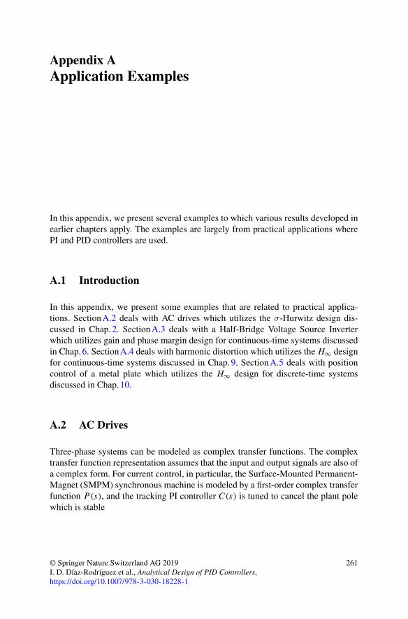
Fig. A.1 Unity feedbackcontrol loop r

C(s)u

P(s)y

−

P(s) := 1

Ls + jωeL + Re−sTd (A.1)

C(s) := k(Ls + jωeL + R)

s. (A.2)

In Fig.A.1, r is the reference current input, u is the voltage input to the plant P(s),and y is themeasured output current. All complex signals and plant and the controllertransfer functions are in the rotating dq frame. ωe is the synchronous frequency, Land R are stator inductance and resistance, Td is the computation and modulationtime delay, and k is a design parameter of the controller.

We set ωe = 50Hz, L = 17.6mH, and R = 2.8 �. We replaced the delay terme−sTd with the second-order Padé approximation. Then, the resulting closed-loopsystem is the same as in Fig. 2.1, where

C(s) = k

s, P(s) = 1 − 1

2Tds + 112T

2d s

2

1 + 12Tds + 1

12T2d s

2. (A.3)

Setting kp = 0, ki = k, and kd = 0 in (2.165), we have

δ′(s ′) = (s ′ − σ)

(1

12T 2d (s ′ − σ)2 + 1

2Td(s

′ − σ) + 1

)

+ k

(1

12T 2d (s ′ − σ)2 − 1

2Td(s

′ − σ) + 1

)

N ′(−s ′) = 1

12T 2d (s ′ + σ)2 + 1

2Td(s

′ + σ) + 1

and

ν ′(s ′) = δ′(s ′)N ′(−s ′)ν ′( jω) = p1(ω,σ, Td) + kp2(ω,σ, Td) + jq(ω,σ, Td),

where

p1(ω,σ, Td) = − 1

12

(1

12σT 4

d − T 3d

)ω4

−(

1

72T 4d σ3 − 1

12T 3d σ2 − 5

12T 2d σ + Td

)ω2

https://doi.org/10.1007/978-3-030-18228-1_2

https://doi.org/10.1007/978-3-030-18228-1_2

Appendix A: Application Examples 263

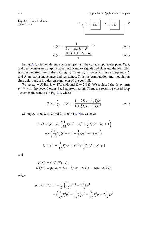
Fig. A.2 Stabilizing kbounds versus σ. © 2018IEEE. Reproduced from [6]with permission

0 500 1000 1500 2000 2500 30000

1000

2000

3000

4000

5000Upper boundLower boundk = 1230

− 1

144T 4d σ5 + 1

12T 2d σ3 − σ,

p2(ω,σ, Td) = 1

144T 4d ω4 + 1

12

(1

6T 4d σ2 + T 3

d σ + T 2d

)ω2

+ 1

144T 4d σ4 + 1

12T 3d σ3 + 5

12T 2d σ2 + Tdσ + 1,

q(ω,σ, Td) = 1

144T 4d ω5 + 1

12

(1

6T 4d σ2 + T 3

d σ − 5T 2d

)ω3

+ 1

12

(1

12T 4d σ4 + T 3

d σ3 − T 2d σ2

)ω + (−Tdσ + 1) ω.

The sets S(σ) are intervals on the k axis and the upper and lower bounds foreach interval with a prescribed σ are plotted in Fig.A.2. S(σ) just becomes empty ataround σ = 3356 and the corresponding k is around 1230.

A.3 Half-Bridge Voltage Source Inverter

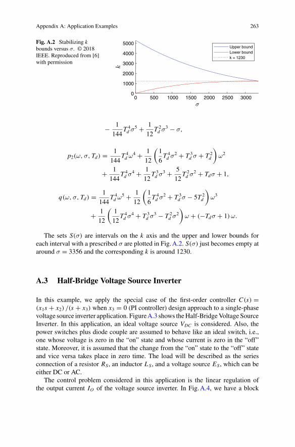
In this example, we apply the special case of the first-order controller C(s) =(x1s + x2) /(s + x3) when x3 = 0 (PI controller) design approach to a single-phasevoltage source inverter application. FigureA.3 shows theHalf-BridgeVoltage SourceInverter. In this application, an ideal voltage source VDC is considered. Also, thepower switches plus diode couple are assumed to behave like an ideal switch, i.e.,one whose voltage is zero in the “on” state and whose current is zero in the “off”state. Moreover, it is assumed that the change from the “on” state to the “off” stateand vice versa takes place in zero time. The load will be described as the seriesconnection of a resistor RS , an inductor LS , and a voltage source ES , which can beeither DC or AC.

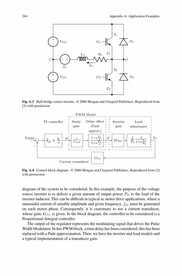
The control problem considered in this application is the linear regulation ofthe output current IO of the voltage source inverter. In Fig.A.4, we have a block


−+

VDC

− +

Es

Ls Rs

IO

−+

VDC

S2

G2

E2

D2

D1

S1

G1

E1

C O

Fig. A.3 Half-bridge source inverter. © 2006 Morgan and Claypool Publishers. Reproduced from[3] with permission

IOREFkp + ki

s

m 1CPK

1−s Ts4

1+s Ts4

d2VDC

1Rs

11+s Ls

Rs

IO

GTI

−

PWM Model

Staticgain

Delay effect(Pade

approx.)

Invertergain

Loadadmittance

PI controller

Current transducer

Fig. A.4 Control block diagram. © 2006 Morgan and Claypool Publishers. Reproduced from [3]with permission

diagram of the system to be considered. In this example, the purpose of the voltagesource inverter is to deliver a given amount of output power PO to the load of theinverter inductor. This can be difficult in typical ac motor drive applications, where asinusoidal current of suitable amplitude and given frequency, fO , must be generatedon each motor phase. Consequently, it is customary to use a current transducer,whose gain, GT I , is given. In the block diagram, the controller to be considered is aProportional–Integral controller.

The output of the regulator represents the modulating signal that drives the PulseWidthModulator. In this PWMblock, a time delay has been considered; this has beenreplaced with a Pade approximation. Then, we have the inverter and load models anda typical implementation of a transducer gain.


A. Computation of the Stabilizing Set

First, the open-loop transfer function is as follows:

GOL(s) = C(s)P(s)

GOL(s) =(kp + ki

s

)2VDC

CPK

1 − s TS4

1 + s TS4

GT I

RS

1

1 + s LSRS

, (A.4)

where VDC = 250 (V), CPK = 4 (V ), T s = 0.00002 (s), GT I = 0.1 (V/A), RS =1 (�), LS = 1.5 (mH). We will consider the notation of the PI controller in (A.4) tobe x1 := kp, x2 := ki , and x3 = 0 for our special case of first-order controller.

We have

GOL(s) =(x1s + x2

s

) −6.25 × 10−5s + 12.5

7.5 × 10−9s2 + 0.0015 s + 1. (A.5)

The closed-loop characteristic polynomial is

δ(s, x1, x2) = 7.5 × 10−9s3 + (0.0015 − 6.25 × 10−5x1)s2

+ (12.5x1 − 6.25 × 10−5x2 + 1)s + 12.5x2. (A.6)

Here, n = 2, m = 1, and N (−s) = 12.5 + 6.25 × 10−5s. Therefore, we obtain

ν(s) = δ(s, x1, x2)N (−s)

= 4.69 × 10−13s4 + (1.87 × 10−7 − 3.91 × 10−9x1)s3

+ (0.0188 − 3.91 × 10−9x2)s2 + (156x1 + 12.5)s + 156x2 (A.7)

so that

ν( jω,x1, x2) = 4.69 × 10−13ω4 + (3.91 × 10−9x2 − 0.0188)ω2 + 156x2

+ j[(3.91 × 10−9x1 − 1.87 × 10−7)ω3 + (156x1 + 12.5)ω]= p(ω) + jq(ω). (A.8)

We find that z+ = 1 so that the signature requirement on ν(s) for stability is

n − m + 1 + 2z+ = 4. (A.9)

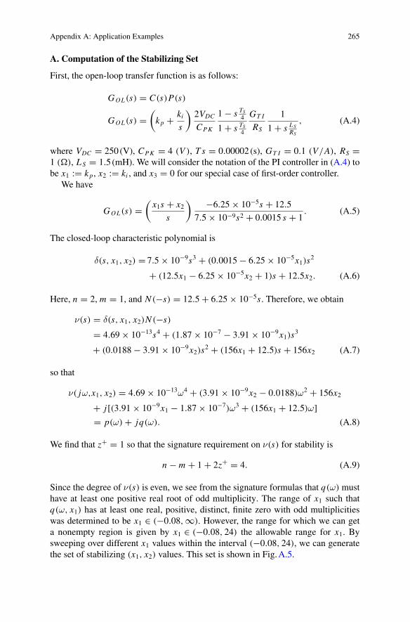
Since the degree of ν(s) is even, we see from the signature formulas that q(ω) musthave at least one positive real root of odd multiplicity. The range of x1 such thatq(ω, x1) has at least one real, positive, distinct, finite zero with odd multiplicitieswas determined to be x1 ∈ (−0.08,∞). However, the range for which we can geta nonempty region is given by x1 ∈ (−0.08, 24) the allowable range for x1. Bysweeping over different x1 values within the interval (−0.08, 24), we can generatethe set of stabilizing (x1, x2) values. This set is shown in Fig.A.5.


0 1 2 3 4 5 6 7 8 9

x2 105

-5

0

5

10

15

20

25

x 1

Fig. A.5 Stability region for −0.08 ≤ x1 ≤ 24

0 20 40 60 80 100 120 140

Phase margin (degree)

100

101

102

103

104

Gai

n m

argi

n

wg = 1000

wg = 3000

wg = 5000

wg = 7000

wg = 9000

wg = 11000

wg = 13000

wg = 15000

wg = 17000

wg = 19000

wg = 21000

wg = 23000

wg = 25000

wg = 27000

wg = 29000

wg = 31000

wg = 33000

wg = 35000

wg = 37000

wg = 39000

wg = 41000

wg = 43000

wg = 45000

wg = 47000

wg = 49000

wg = 51000

wg = 53000

wg = 55000

wg = 57000

wg = 59000

wg = 61000

wg = 63000

wg = 65000

wg = 67000

wg = 69000

PM: 34GM: 5327

PM: 120GM: 167

PM: 9.003GM: 267.3

PM: 14GM: 746

PM: 100GM: 65.28

PM: 94GM: 39.77

PM: 60GM: 3.768

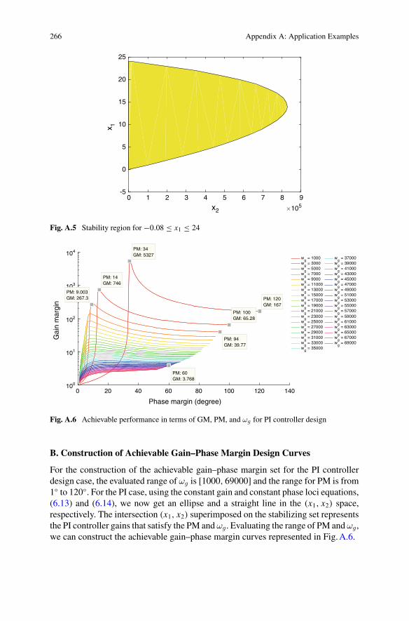
Fig. A.6 Achievable performance in terms of GM, PM, and ωg for PI controller design

B. Construction of Achievable Gain–Phase Margin Design Curves

For the construction of the achievable gain–phase margin set for the PI controllerdesign case, the evaluated range of ωg is [1000, 69000] and the range for PM is from1◦ to 120◦. For the PI case, using the constant gain and constant phase loci equations,(6.13) and (6.14), we now get an ellipse and a straight line in the (x1, x2) space,respectively. The intersection (x1, x2) superimposed on the stabilizing set representsthe PI controller gains that satisfy the PM andωg. Evaluating the range of PM andωg,we can construct the achievable gain–phase margin curves represented in Fig.A.6.

https://doi.org/10.1007/978-3-030-18228-1_6

https://doi.org/10.1007/978-3-030-18228-1_6


C. Simultaneous Performance Specifications and Retrieval of Controller Gains

In Fig.A.6, we display the achievable gain–phase margin set of curves indexed bya fixed ωg in different colors. Notice that we can get more GM and PM for lowervalues of ωg . For example, for ωg = 1000 rad/s, the maximum GM that we can getis 5327 with a PM of 34◦. For ωg = 3000 rad/s, the maximum GM is 746 with aPM = 14◦. Using Fig.A.6, the designer has the liberty to choose values for GM,PM, and ωg that best suits his design needs.

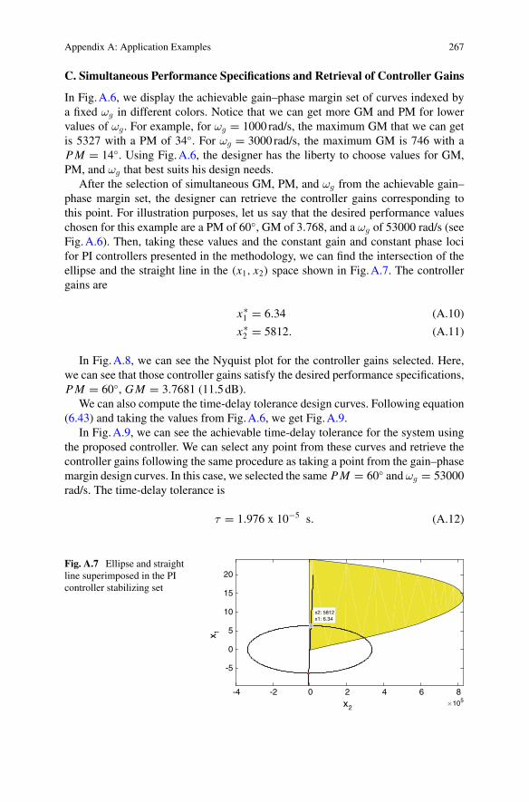
After the selection of simultaneous GM, PM, and ωg from the achievable gain–phase margin set, the designer can retrieve the controller gains corresponding tothis point. For illustration purposes, let us say that the desired performance valueschosen for this example are a PM of 60◦, GM of 3.768, and a ωg of 53000 rad/s (seeFig.A.6). Then, taking these values and the constant gain and constant phase locifor PI controllers presented in the methodology, we can find the intersection of theellipse and the straight line in the (x1, x2) space shown in Fig.A.7. The controllergains are

x∗1 = 6.34 (A.10)

x∗2 = 5812. (A.11)

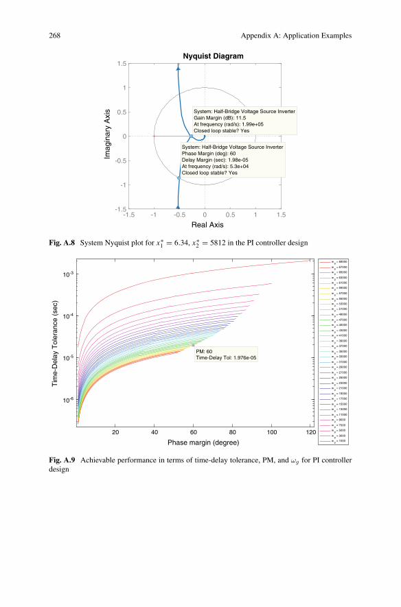
In Fig.A.8, we can see the Nyquist plot for the controller gains selected. Here,we can see that those controller gains satisfy the desired performance specifications,PM = 60◦, GM = 3.7681 (11.5dB).

We can also compute the time-delay tolerance design curves. Following equation(6.43) and taking the values from Fig.A.6, we get Fig.A.9.

In Fig.A.9, we can see the achievable time-delay tolerance for the system usingthe proposed controller. We can select any point from these curves and retrieve thecontroller gains following the same procedure as taking a point from the gain–phasemargin design curves. In this case, we selected the same PM = 60◦ and ωg = 53000rad/s. The time-delay tolerance is

τ = 1.976 x 10−5 s. (A.12)

Fig. A.7 Ellipse and straightline superimposed in the PIcontroller stabilizing set

-4 -2 0 2 4 6 8x2

105

-5

0

5

10

15

20

x 1

x2: 5812x1: 6.34

https://doi.org/10.1007/978-3-030-18228-1_6


-1.5 -1 -0.5 0 0.5 1 1.5-1.5

-1

-0.5

0

0.5

1

1.5Nyquist Diagram

Real Axis

Imag

inar

y A

xis System: Half-Bridge Voltage Source Inverter

Gain Margin (dB): 11.5 At frequency (rad/s): 1.99e+05Closed loop stable? Yes

System: Half-Bridge Voltage Source InverterPhase Margin (deg): 60 Delay Margin (sec): 1.98e-05 At frequency (rad/s): 5.3e+04Closed loop stable? Yes

Fig. A.8 System Nyquist plot for x∗1 = 6.34, x∗

2 = 5812 in the PI controller design

20 40 60 80 100 120

Phase margin (degree)

10-6

10-5

10-4

10-3

Tim

e-D

elay

Tol

eran

ce (

sec)

wg = 69000

wg = 67000

wg = 65000

wg = 63000

wg = 61000

wg = 59000

wg = 57000

wg = 55000

wg = 53000

wg = 51000

wg = 49000

wg = 47000

wg = 45000

wg = 43000

wg = 41000

wg = 39000

wg = 37000

wg = 35000

wg = 33000

wg = 31000

wg = 29000

wg = 27000

wg = 25000

wg = 23000

wg = 21000

wg = 19000

wg = 17000

wg = 15000

wg = 13000

wg = 11000

wg = 9000

wg = 7000

wg = 5000

wg = 3000

wg = 1000

PM: 60Time-Delay Tol: 1.976e-05

Fig. A.9 Achievable performance in terms of time-delay tolerance, PM, and ωg for PI controllerdesign


A.4 Selective Mitigation of Harmonic Distortion

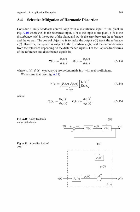
Consider a unity feedback control loop with a disturbance input to the plant inFig.A.10 where r(t) is the reference input, u(t) is the input to the plant, ξ(t) is thedisturbance, y(t) is the output of the plant, and e(t) is the error between the referenceand the output. The control objective is to make the output y(t) track the referencer(t). However, the system is subject to the disturbance ξ(t) and the output deviatesfrom the reference depending on the disturbance signals. Let the Laplace transformsof the reference and disturbance signals be

R(s) := nr (s)

dr (s), �(s) := nξ(s)

dξ(s), (A.13)

where nr (s), dr (s), nξ(s), dξ(s) are polynomials in s with real coefficients.We assume that (see Fig.A.11)

Y (s) = [Pu(s) Pξ(s)

]︸︷︷︸

=:P(s)

[U (s)�(s),

](A.14)

where

Pu(s) = nPu(s)

dPu(s)

, Pξ(s) = nPξ(s)

dPξ(s)

. (A.15)

Fig. A.10 Unity feedbackunder disturbance

r(t) + e(t)C(s)

u(t)P (s)

y(t)

−

ξ(t)

Fig. A.11 A detailed look ofP(s)

u(t) Pu(s)yu(t) +

y(t)

yξ(t)

+

Pξ(s)

ξ(t)

P (s)


Assumption A.1 dPu(s) = dPξ

(s).

Since

E(s) = R(s) − Y (s), (A.16)

U (s) = C(s)E(s), (A.17)

where

C(s) = nC(s)

dC(s)(A.18)

we have by AssumptionA.1 that

E(s) = dPu(s)dC(s)

dcl(s)R(s) − dPu

(s)dC(s)nPξ(s)

dcl(s)�(s), (A.19)

where the closed-loop characteristic polynomial is

dcl(s) = dC(s)dP(s) + nC(s)nP(s). (A.20)

Assumption A.2 C(s) is of a PID type.

By AssumptionA.2, yu(t) tracks the arbitrary constant reference input r(t) inthe steady state provided that the closed loop is stable. Since e(t) = r(t) − y(t),e(t) → yξ(t) as t → ∞. Thus, the error signal only has the closed-loop responseto the disturbance ξ(t) in the steady state. Let Yξ(s) be the Laplace transform ofyξ(t) and the disturbance ξ(t) be a linear combination of sinusoidal signals of fixedfrequencies, say ω1, . . . ,ωq

ξ(t) =q∑

i=1

ξi (t) =q∑

i=1

Aisin(ωi t), (A.21)

where Ai is the amplitude of i th sinusoidal. If the frequencies of signals are multiplesof a fundamental frequency, say ω1, we call each signal ξi (t) a harmonic of ξ1(t).

∣∣Yξ( jωi )∣∣ =

∣∣∣∣ Pξ( jωi )

1 + C( jωi )Pu( jωi )

∣∣∣∣ Ai (A.22)

Let γ̃i be a prescribed upper bound for the amplitude of yξ(t) at frequency ωi , thatis, ∣∣Yξ( jωi )

∣∣ < γ̃i . (A.23)


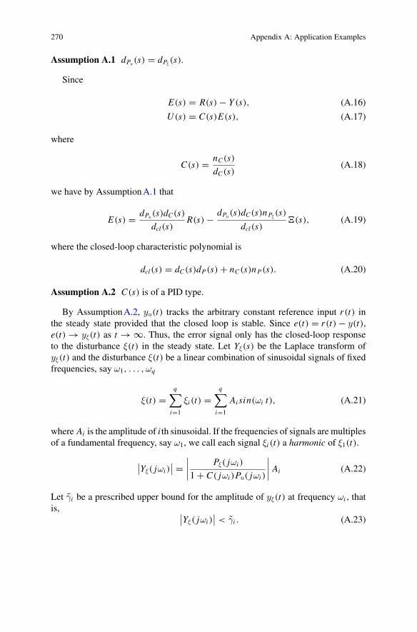
Fig. A.12 The stabilizingcontrollers satisfying theharmonic mitigation are theintersection of the outside ofthe ellipses and inside thestabilizing set

ki

kp

Stabilizing set|Su(jω1)| = γ1

|Su(jω2)| = γ2 |Su(jω3)| = γ3

Then,

∣∣Yξ( jωi )∣∣ < γ̃i ⇔

∣∣∣∣ 1

1 + C( jωi )Pu( jωi )

∣∣∣∣︸︷︷︸=:Su( jωi )

<γ̃i∣∣Pξ( jωi )

∣∣ Ai︸︷︷︸=:γi

⇔ |1 + C( jωi )Pu( jωi )| >1

γi.

(A.24)

Thus, it is possible to design a stabilizing controller that compensates each harmonicpresent in the disturbance.

In the sequel, we graphically design a PI controller that renders the closed-loopsystem to have the frequency response of the error signal less than a prescribedvalue γi at each fixed frequency ωi . This is illustrated in Fig.A.12. The stabilizingcontrollers are simultaneously outside of the ellipses (dashed lines) and inside of thestabilizing set (solid line).

Let us consider the following continuous-time LTI plant:

Pu(s) = s − 5

10 s2 + 16 s + 2, (A.25)

and the disturbance transfer function:

Pξ(s) = 20 s2 + 8 s + 1

10 s2 + 16 s + 2. (A.26)

Suppose that the controller to be designed is a PI controller given by

C(s) = kp + kis

, (A.27)

the reference input for this system is a unit step and it is subject to a disturbancesignal ξ(t) = ξ1(t) + ξ2(t) with


ξ1(t) = 0.6 sin(2t) (A.28)

ξ2(t) = 0.4 sin(3t). (A.29)

Suppose also that the specifications to be attained are

• Amplitude of the harmonic at 2 rad/s is less than 2.• Amplitude of the harmonic at 3 rad/s is less than 2.

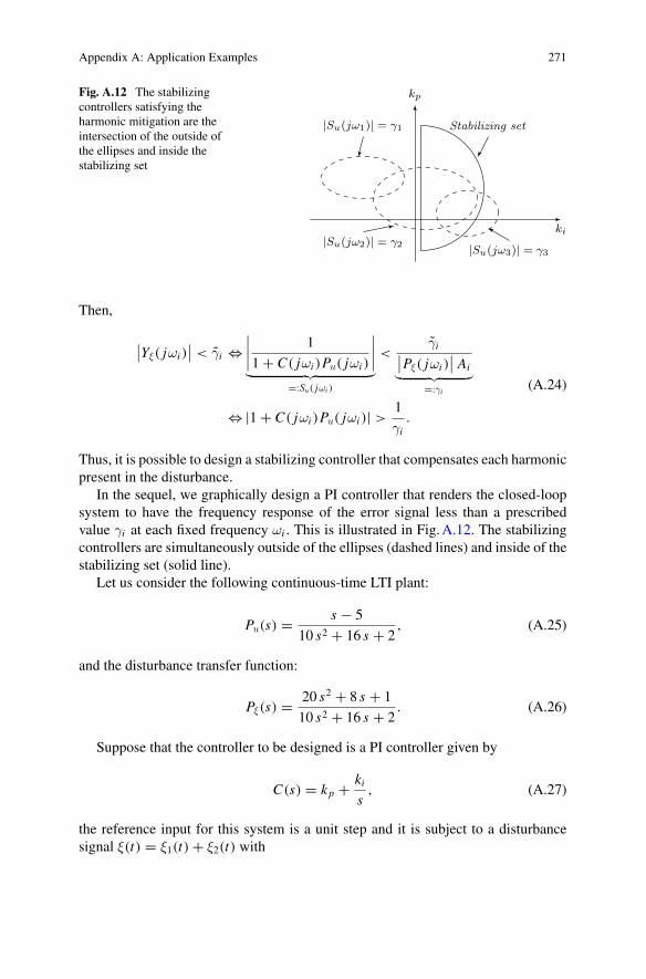
The stabilizing set of PI controllers for the given plant is computed first. Fromthe disturbance signal characterization, we identify that A1 = 0.6, A2 = 0.4, ω1 =2 rad/s, and ω2 = 3 rad/s. From the specifications, we have γ̃1 = 2 and γ̃2 = 2.Substituting (9.28) and (9.29) into (A.24), we obtain that γ1 ≈ 2.0544, γ2 ≈ 2.7752,and the set of all possible controllers in the stabilizing set attaining the specifications.This is shown in Fig.A.13. We select four sample points, shown in TableA.1, andexamine whether or not the chosen controllers achieve the specifications.

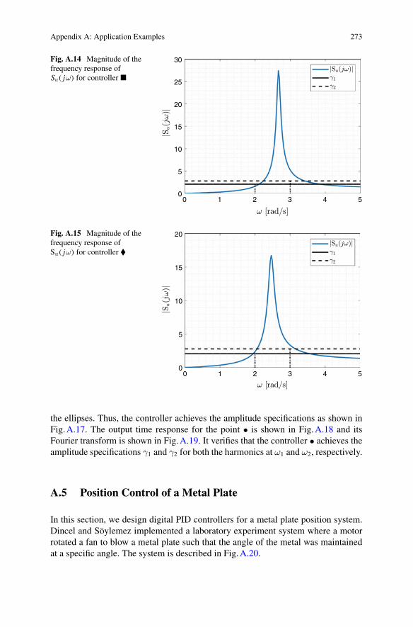
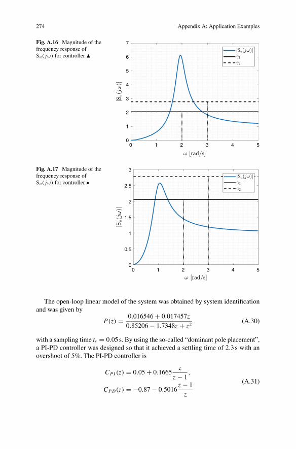
The controller� lies outside of the ellipse |Su( jω1)| = γ1 but inside of the ellipse|Su( jω2)| = γ2. The controller guarantees yξ(t) to have the harmonic amplitude lessthan 2 at ω1 but not for ω2 as shown in Fig.A.14. The controller � lies inside of theellipse |Su( jω1) = γ1| and the ellipse |Su( jω2)| = γ2. This means that the controllerdoes not guarantee any of the amplitude specifications. This is shown in Fig.A.15.The controller � lies inside of the ellipse |Su( jω1)| = γ1 and outside of the ellipse|Su( jω2)| = γ2. This controller achieves the amplitude specification for the harmonicat ω2 but not for ω1 as shown in Fig.A.16. The controller • lies outside of both

Fig. A.13 Stabilizing setwith harmonic mitigationspecifications

-20 -10 0 10 20-25

-20

-15

-10

-5

0

Table A.1 Selected controllers

� � � •kp −14.0861 −12.2734 −7.9683 −2.7568

ki −1.1521 −2.4424 −3.0876 −1.5207

https://doi.org/10.1007/978-3-030-18228-1_9

https://doi.org/10.1007/978-3-030-18228-1_9


Fig. A.14 Magnitude of thefrequency response ofSu( jω) for controller �

0

5

10

15

20

25

30

0 1 2 3 4 5


0 1 2 3 4 50

5

10

15

20

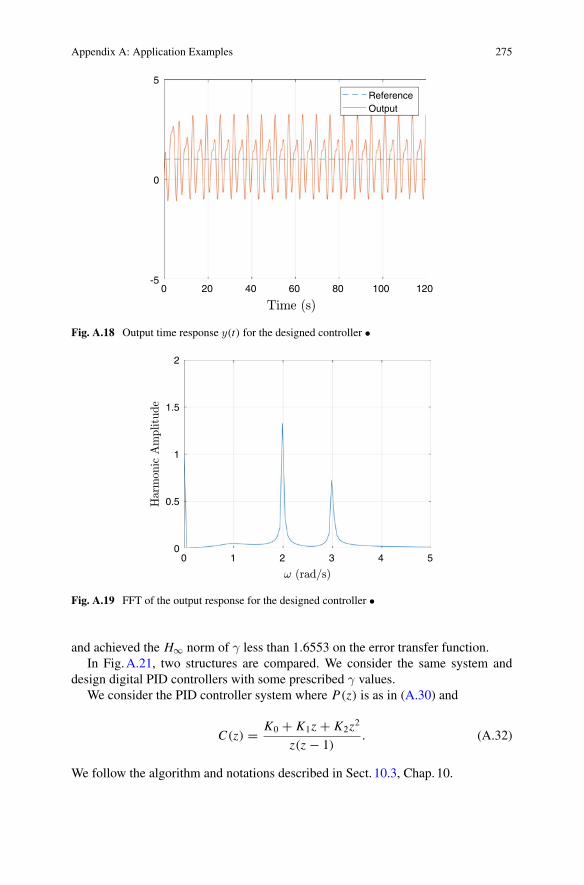
the ellipses. Thus, the controller achieves the amplitude specifications as shown inFig.A.17. The output time response for the point • is shown in Fig.A.18 and itsFourier transform is shown in Fig.A.19. It verifies that the controller • achieves theamplitude specifications γ1 and γ2 for both the harmonics at ω1 and ω2, respectively.

A.5 Position Control of a Metal Plate

In this section, we design digital PID controllers for a metal plate position system.Dincel and Söylemez implemented a laboratory experiment system where a motorrotated a fan to blow a metal plate such that the angle of the metal was maintainedat a specific angle. The system is described in Fig.A.20.



0 1 2 3 4 50

1

2

3

4

5

6

7

Fig. A.17 Magnitude of thefrequency response ofSu( jω) for controller •

0 1 2 3 4 50

0.5

1

1.5

2

2.5

3

The open-loop linear model of the system was obtained by system identificationand was given by

P(z) = 0.016546 + 0.017457z

0.85206 − 1.7348z + z2(A.30)

with a sampling time ts = 0.05s. By using the so-called “dominant pole placement”,a PI-PD controller was designed so that it achieved a settling time of 2.3s with anovershoot of 5%. The PI-PD controller is

CPI (z) = 0.05 + 0.1665z

z − 1,

CPD(z) = −0.87 − 0.5016z − 1

z

(A.31)


0 20 40 60 80 100 120-5

0

5

ReferenceOutput

Fig. A.18 Output time response y(t) for the designed controller •

0 1 2 3 4 50

0.5

1

1.5

2

Fig. A.19 FFT of the output response for the designed controller •

and achieved the H∞ norm of γ less than 1.6553 on the error transfer function.In Fig.A.21, two structures are compared. We consider the same system and

design digital PID controllers with some prescribed γ values.We consider the PID controller system where P(z) is as in (A.30) and

C(z) = K0 + K1z + K2z2

z(z − 1). (A.32)

We follow the algorithm and notations described in Sect. 10.3, Chap. 10.

https://doi.org/10.1007/978-3-030-18228-1_10


Metal plate

Angle measured by a potentiometer

MotorFan

Fig. A.20 A metal plate system

Fig. A.21 a Digital PI-PDcontroller structure, b DigitalPID controller structure

r[k] +CPI(z)

+P (z)

y[k]

CPD(z)

−−

(a)

r[k] +C(z) P (z)

y[k]

−

(b)

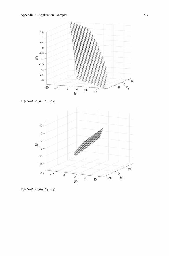
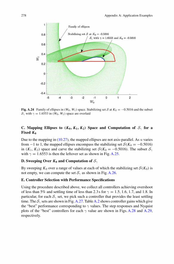
A. Computation of the Stabilizing Set SThe stabilizing set S for PID controllers in (K1, K2, K3) space is described inChap.4. Since K3 := K2 − K0, we can convert the stabilizing set S(K1, K2, K3)

into S(K0, K1, K2) using the following relationship

⎡⎣K0

K1

K2

⎤⎦ =

⎡⎣0 1 −11 0 00 1 0

⎤⎦

⎡⎣K1

K2

K3

⎤⎦ . (A.33)

Two stabilizing sets are shown in Figs.A.22 and A.23.

B. Computation of Family of Ellipses in (W0,W1) Space

Let us first choose γ = 1.6553 and K0 = −0.5016 since the PI-PD controller in(A.31) renders the H∞ norm less than 1.6533 and the constant term in the numeratorof the PD controller is equal to −0.5016. Since the ellipse in (10.43) is an axis-parallel ellipse, the family of ellipses must be a collection of axis-parallel ellipses in(W0,W1) space as shown in Fig.A.24. The stabilizing set S at K0 = −0.5016 andthe subset Sγ with γ = 1.6553 space are to be determined in the next step.

https://doi.org/10.1007/978-3-030-18228-1_4

https://doi.org/10.1007/978-3-030-18228-1_10


Fig. A.22 S(K1, K2, K3)

Fig. A.23 S(K0, K1, K2)


Fig. A.24 Family of ellipses in (W0,W1) space. Stabilizing set S at K0 = −0.5016 and the subsetSγ with γ = 1.6553 in (W0,W1) space are overlaid

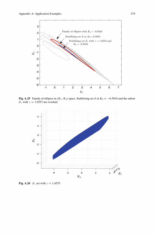
C. Mapping Ellipses to (K0, K1, K2) Space and Computation of Sγ for aFixed K0

Due to the mapping in (10.27), the mapped ellipses are not axis-parallel. As u variesfrom −1 to 1, the mapped ellipses encompass the stabilizing set S(K0 = −0.5016)in (K1, K2) space and carve the stabilizing set S(K0 = −0.5016). The subset Sγ

with γ = 1.6553 is then the leftover set as shown in Fig.A.25.

D. Sweeping Over K0 and Computation of Sγ

By sweeping K0 over a range of values at each of which the stabilizing set S(K0) isnot empty, we can compute the set Sγ as shown in Fig.A.26.

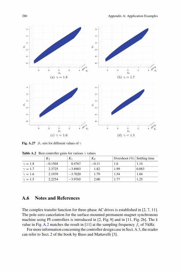
E. Controller Selection with Performance Specifications

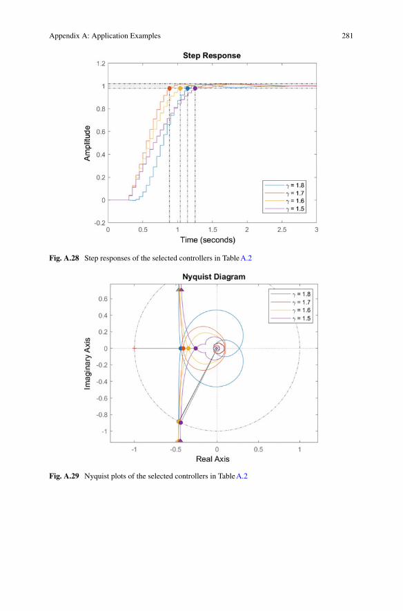
Using the procedure described above, we collect all controllers achieving overshootof less than 5% and settling time of less than 2.3s for γ = 1.5, 1.6, 1.7, and 1.8. Inparticular, for each Sγ set, we pick such a controller that provides the least settlingtime. TheSγ sets are shown in Fig.A.27. TableA.2 shows controller gains which givethe “best” performance corresponding to γ values. The step responses and Nyquistplots of the “best” controllers for each γ value are shown in Figs.A.28 and A.29,respectively.

https://doi.org/10.1007/978-3-030-18228-1_10


-1 0 1 2 3 4 5 6 7-6

-5

-4

-3

-2

-1

0

1

2

3

Fig. A.25 Family of ellipses in (K1, K2) space. Stabilizing set S at K0 = −0.5016 and the subsetSγ with γ = 1.6553 are overlaid

Fig. A.26 Sγ set with γ = 1.6553


(a) γ = 1.8 (b) γ = 1.7

(c) γ = 1.6 (d) γ = 1.5

Fig. A.27 Sγ sets for different values of γ

Table A.2 Best controller gains for various γ values

K2 K1 K0 Overshoot (%) Settling time

γ = 1.8 −0.1504 0.4767 −0.11 1.6 1.14

γ = 1.7 2.3725 −3.8903 1.82 1.99 0.883

γ = 1.6 2.1939 −3.7020 1.79 1.54 1.04

γ = 1.5 2.2254 −3.9765 2.00 1.77 1.25

A.6 Notes and References

The complex transfer function for three-phase AC drives is established in [2, 7, 11].The pole-zero cancelation for the surface-mounted permanent-magnet synchronousmachine using PI controllers is introduced in [2, Fig. 9] and in [11, Fig. 2b]. The kvalue in Fig.A.2 matches the result in [11] at the sampling frequency fs of 5kHz.

Formore information concerning the controller design case in Sect.A.3, the readercan refer to Sect. 2 of the book by Buso and Mattavelli [3].


Fig. A.28 Step responses of the selected controllers in TableA.2

Fig. A.29 Nyquist plots of the selected controllers in TableA.2


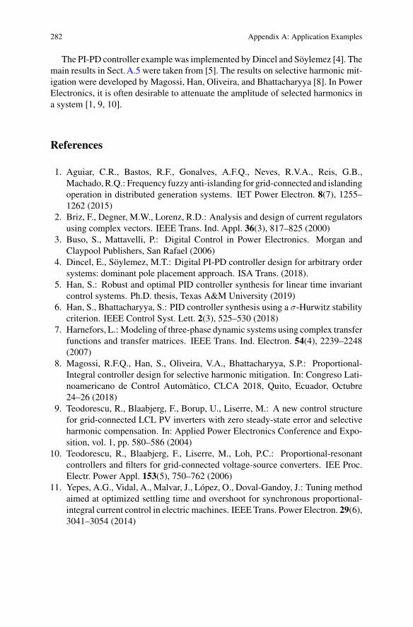
The PI-PD controller example was implemented byDincel and Söylemez [4]. Themain results in Sect.A.5 were taken from [5]. The results on selective harmonic mit-igation were developed by Magossi, Han, Oliveira, and Bhattacharyya [8]. In PowerElectronics, it is often desirable to attenuate the amplitude of selected harmonics ina system [1, 9, 10].

References

1. Aguiar, C.R., Bastos, R.F., Gonalves, A.F.Q., Neves, R.V.A., Reis, G.B.,Machado,R.Q.: Frequency fuzzy anti-islanding for grid-connected and islandingoperation in distributed generation systems. IET Power Electron. 8(7), 1255–1262 (2015)

2. Briz, F., Degner, M.W., Lorenz, R.D.: Analysis and design of current regulatorsusing complex vectors. IEEE Trans. Ind. Appl. 36(3), 817–825 (2000)

3. Buso, S., Mattavelli, P.: Digital Control in Power Electronics. Morgan andClaypool Publishers, San Rafael (2006)

4. Dincel, E., Söylemez, M.T.: Digital PI-PD controller design for arbitrary ordersystems: dominant pole placement approach. ISA Trans. (2018).

5. Han, S.: Robust and optimal PID controller synthesis for linear time invariantcontrol systems. Ph.D. thesis, Texas A&M University (2019)

6. Han, S., Bhattacharyya, S.: PID controller synthesis using a σ-Hurwitz stabilitycriterion. IEEE Control Syst. Lett. 2(3), 525–530 (2018)

7. Harnefors, L.: Modeling of three-phase dynamic systems using complex transferfunctions and transfer matrices. IEEE Trans. Ind. Electron. 54(4), 2239–2248(2007)

8. Magossi, R.F.Q., Han, S., Oliveira, V.A., Bhattacharyya, S.P.: Proportional-Integral controller design for selective harmonic mitigation. In: Congreso Lati-noamericano de Control Automàtico, CLCA 2018, Quito, Ecuador, Octubre24–26 (2018)

9. Teodorescu, R., Blaabjerg, F., Borup, U., Liserre, M.: A new control structurefor grid-connected LCL PV inverters with zero steady-state error and selectiveharmonic compensation. In: Applied Power Electronics Conference and Expo-sition, vol. 1, pp. 580–586 (2004)

10. Teodorescu, R., Blaabjerg, F., Liserre, M., Loh, P.C.: Proportional-resonantcontrollers and filters for grid-connected voltage-source converters. IEE Proc.Electr. Power Appl. 153(5), 750–762 (2006)

11. Yepes, A.G., Vidal, A., Malvar, J., López, O., Doval-Gandoy, J.: Tuning methodaimed at optimized settling time and overshoot for synchronous proportional-integral current control in electric machines. IEEE Trans. Power Electron. 29(6),3041–3054 (2014)

Appendix BSample MATLAB Codes

We present sample MATLAB codes and the associated figures. The purpose is tohelp the readers to understand the results developed and used in this book. Moreover,they can readily apply the codes to their research problems as a starting point. Werecommend readers to use the latest version of the MATLAB software.

B.1 Sample MATLAB Codes for Continuous-TimeSystems

We present how to graphically visualize the stabilizing set of PI and PID controllersfor a given continuous-time system. The mathematical account of the stabilizing setis discussed in Part I. The computation of the stabilizing set is a foundation of all ofthe design methods we developed in the rest of this book. Following the stabilizingset, we provide how to get the design curves for gain and phase margin design inPart II. Next, we show the MATLAB codes for all stabilizing PI and PID controllerssatisfying an H∞ criterion in Part III.

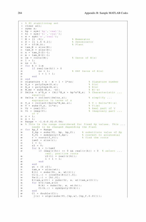
B.1.1 PI Controller Stabilizing Set

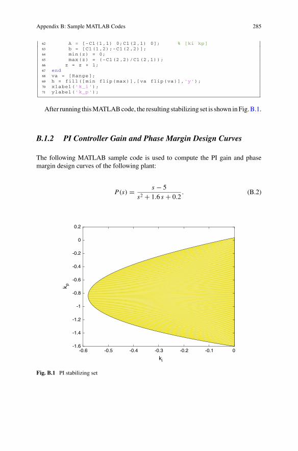
The following MATLAB sample code is used to compute the PI stabilizing set of thefollowing plant:

P(s) = s − 5

s2 + 1.6 s + 0.2. (B.1)


283

https://doi.org/10.1007/978-3-030-18228-1

284 Appendix B: Sample MATLAB Codes

1 % PI stabilizing set2 clear all;3 syms s;4 kp = sym('kp','real');5 ki = sym('ki','real');6 w = sym('w','real');7 N = [1 -5]; % Numerator8 D = [1 1.6 0.2]; % Denominator9 P = tf(N,D); % Plant10 tam_N = size(N);11 tam_D = size(D);12 n = tam_D (2) -1;13 m = tam_N (2) -1;14 ze = roots(N); % Zeros of N(s)15 l = 1;16 nz = 0;17 for k = 1:m18 if real(ze(k)) > 019 nz = l; % RHP Zeros of N(s)20 l = l + 1;21 end22 end23 signature = n - m + 1 + 2*nz; % Signature number24 D_s = poly2sym(D,s); % D(s)25 N_s = poly2sym(N,s); % N(s)26 N_ms = subs(N_s , -s); % N(-s)27 Delta = s*D_s + (ki)*N_s + kp*s*N_s; % Characteristic ...

equation28 Delta = collect(Delta ,s); % simplify ...

expression in terms of s29 V_s = collect(Delta*N_ms ,s); % V = Delta*N(-s)30 V = subs(V_s , 1i*w); % V(jw)31 Vr = real(V); % Real part of V32 Vi = imag(V); % Imaginary part ...

of V33 z = 1;34 e = 1;35 Range = -1.6:0.01:0.04;36 % This is the range considered for fixed Kp values. This ...

needs to be changed depending the Plant37 for kp_f = Range38 f_kp = subs(Vi , kp , kp_f); % substitute value of Kp39 f_Vi = sym2poly(f_kp); % convert to polynomial40 r = roots(f_Vi); % find the roots41 tam3 = size(r);42 l = 1;43 r2 = 0;44 for k = 1:tam345 if imag(r(k)) == 0 && real(r(k)) > 0 % select ...

real , positive roots46 r2(l) = real(r(k));47 l = l + 1;48 end49 end50 wt = [0 r2];51 tam_w = size(wt);52 R(1) = subs(Vr , w, wt(1));53 C1(1,:) = [coeffs(R(1)) ,0];54 Te(1,:) = [ki ,0];55 R(tam_w (2)) = subs(Vr, w, wt(tam_w (2)));56 for k=2: tam_w (2)57 R(k) = subs(Vr , w, wt(k));58 C1(k,:) = sym2poly(R(k));59 end60 C1 = double(C1);61 j(z) = sign(subs(Vi ,[kp ,w],[kp_f ,0.01]));

Appendix B: Sample MATLAB Codes 285

62 A = [-C1(1,1) 0;C1(2,1) 0]; % [ki kp]63 b = [C1(1,2);-C1(2,2)];64 min(z) = 0;65 max(z) = (-C1(2,2)/C1(2,1));66 z = z + 1;67 end68 va = [Range ];69 h = fill([min flip(max)],[va flip(va)],'y');70 xlabel('k_i');71 ylabel('k_p');

After running thisMATLABcode, the resulting stabilizing set is shown inFig.B.1.

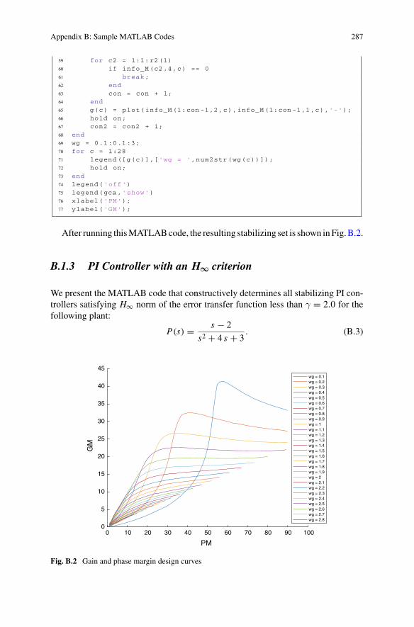
B.1.2 PI Controller Gain and Phase Margin Design Curves

The following MATLAB sample code is used to compute the PI gain and phasemargin design curves of the following plant:

P(s) = s − 5

s2 + 1.6 s + 0.2. (B.2)

-0.6 -0.5 -0.4 -0.3 -0.2 -0.1 0

ki

-1.6

-1.4

-1.2

-1

-0.8

-0.6

-0.4

-0.2

0

0.2

k p

Fig. B.1 PI stabilizing set


1 %% Gain and Phase Margin Design Curves2 N = [1 -5]; % Numerator of the plant3 D = [1 1.6 0.2]; % Denominator of the plant4 P = tf(N,D); % Plant5 PM = [1:90]; % Phase margin range6 z = 1;7 z2 = 1;8 z4 = 1;9 r = size(PM);10 for wg = 0.1:0.1:3 % Gain crossover frequency range11 z = 1;12 for k = 1:1:r(2)13 [MP,PP] = bode(P,wg);14 syms kp;15 syms ki;16 phi = pi + PM(k)*pi/180 - PP*pi/180;17 m2 = 1/(MP^2);18 m = sqrt(m2);19 a2 = m2;20 b2 = m2*(wg^2);21 c = wg*tan(phi);22 f1(z4) = ((kp)^2)/(a2) + (ki^2)/(b2) - 1;23 f2(z4) = kp*c + ki;24 hold on;25 X = solve([f1(z4) , f2(z4) ], [kp, ki]);26 z4 = z4 + 1;27 x1_1 = double(X.kp (1));28 x1_2 = double(X.ki (1));29 x2_1 = double(X.kp (2));30 x2_2 = double(X.ki (2));31 C1 = tf([x2_1 x2_2],[1 0]);32 S1 = allmargin(C1*P);33 E2 = S1.Stable;34 C2 = tf([x1_1 x1_2],[1 0]);35 S2 = allmargin(C2*P);36 E1 = S2.Stable;37 if E1 == 138 R_E1 = allmargin(C2*P);39 [Gm2(z),Pm2(z),Wgm2(z),Wpm2(z)] = margin(C2*P);40 Gm_dB2(z) = 20* log10(Gm2(z));41 info_M(z,:,z2) = ...

[Gm_dB2(z),Pm2(z),Wgm2(z),Wpm2(z),R_E1.DelayMargin ];42 end43 if E2 == 144 [Gm1(z),Pm1(z),Wgm1(z),Wpm1(z)] = margin(C1*P);45 R_E2 = allmargin(C1*P);46 Gm_dB1(z) = 20* log10(Gm1(z));47 info_M(z,:,z2) = ...

[Gm_dB1(z),Pm1(z),Wgm1(z),Wpm1(z),R_E2.DelayMargin ];48 end49 z = z + 1;50 end51 z2 = z2 + 1;52 end53 %% Plot of the PM vs GM design curves54 figure (1)55 r2 = size(info_M);56 con2 = 1;57 for c = 1:1:r2(3)58 con = 1;


59 for c2 = 1:1:r2(1)60 if info_M(c2 ,4,c) == 061 break;62 end63 con = con + 1;64 end65 g(c) = plot(info_M (1:con -1,2,c),info_M (1:con -1,1,c),'-');66 hold on;67 con2 = con2 + 1;68 end69 wg = 0.1:0.1:3;70 for c = 1:2871 legend ([g(c)],['wg = ',num2str(wg(c))]);72 hold on;73 end74 legend('off')75 legend(gca ,'show')76 xlabel('PM');77 ylabel('GM');


B.1.3 PI Controller with an H∞ criterion

We present the MATLAB code that constructively determines all stabilizing PI con-trollers satisfying H∞ norm of the error transfer function less than γ = 2.0 for thefollowing plant:

P(s) = s − 2

s2 + 4 s + 3. (B.3)

0 10 20 30 40 50 60 70 80 90 100

PM

0

5

10

15

20

25

30

35

40

45

GM

wg = 0.1wg = 0.2wg = 0.3wg = 0.4wg = 0.5wg = 0.6wg = 0.7wg = 0.8wg = 0.9wg = 1wg = 1.1wg = 1.2wg = 1.3wg = 1.4wg = 1.5wg = 1.6wg = 1.7wg = 1.8wg = 1.9wg = 2wg = 2.1wg = 2.2wg = 2.3wg = 2.4wg = 2.5wg = 2.6wg = 2.7wg = 2.8

Fig. B.2 Gain and phase margin design curves


1 close all;2 clear;3 syms s;4 % plant5 N = [1 -2]; % Numerator6 D = [1 4 3]; % Denominator7 P_tf=tf(N,D);8 N_s=poly2sym(N,s);9 D_s=poly2sym(D,s);10 P=N_s/D_s;11 theta_rad=-pi:0.01:pi;12 resol =0.01;13

14 % 1. Load the stabilizing set15 % We assume the stabilizing set is readily available16 load stab_pi_plant_00.mat;17 stabset = [[ Ki_bounds (:,1); flipud(Ki_bounds (:,2))], ...18 [Kp_range; flipud(Kp_range);]];19 poly_stabset = ...

simplify(polyshape(stabset ,'Simplify ',false));20 clear Ki_bounds Kp_range;21

22 % 2. Initial Sgamma is the stabilizing set23 poly_Sgamma = poly_stabset;24

25 % 3. Fix gamma and constructively determine S gamma set26 gamma =2.0;27 w_freqs=linspace (0.01 ,3.0 ,300);28 for idx = 1: numel(w_freqs)29 w=w_freqs(idx);30 Pr=double(real(subs(P,s,1i*w)));31 Pi=double(imag(subs(P,s,1i*w)));32 % (x - c1)^2 / a^2 + (y - c2)^2 / b^2 = 133 c1 = -(w*Pi)/(Pr^2 + Pi^2);34 c2 = -Pr/(Pr^2 + Pi^2);35 bb = 1/(( gamma ^2)*(Pr^2 + Pi^2));36 aa = (w^2)*bb;37 x=c1+sqrt(aa)*cos(theta_rad);38 y=c2+sqrt(bb)*sin(theta_rad);39

40 poly_Sgamma = ...subtract(poly_Sgamma ,polyshape(x,y,'Simplify ',true));

41 end42

43 % 4. Collect sample ellipses for display (optional)44 clear idx w_freqs w Pr Pi;45 gamma =2;46 w_freqs =0.1:0.2:5;47 coords_x = NaN(numel(w_freqs),numel(theta_rad));48 coords_y = NaN(numel(w_freqs),numel(theta_rad));49 parfor idx = 1:numel(w_freqs)50 w=w_freqs(idx);51 Pr=real(subs(P,s,1i*w));52 Pi=imag(subs(P,s,1i*w));53 % (x - c1)^2 / a^2 + (y - c2)^2 / b^2 = 154 c1 = -(w*Pi)/(Pr^2 + Pi^2);55 c2 = -Pr/(Pr^2 + Pi^2);56 bb = 1/(( gamma ^2)*(Pr^2 + Pi^2));57 aa = (w^2)*bb;58 x=c1+sqrt(aa)*cos(theta_rad);59 y=c2+sqrt(bb)*sin(theta_rad);60 coords_x(idx ,:)=x;61 coords_y(idx ,:)=y;62 end63

64 figure;


65 fill(poly_stabset.Vertices (:,1), ...66 poly_stabset.Vertices (:,2),'y');67 hold on;68 plot(poly_Sgamma.Vertices (:,1), ...69 poly_Sgamma.Vertices (:,2),'-',...70 'LineWidth ',2, 'Color ', [0 0 0]);71 for idx = 1:size(coords_x ,1)72 x=coords_x(idx ,:) ';73 y=coords_y(idx ,:) ';74 plot(x,y,'k:');75 end76 xlabel('$$k_i$$ ','interpreter ','latex ');77 ylabel('$$k_p$$ ','interpreter ','latex ');78 axis([-4.4 1.2 -4.5 2.0]);79 str = '$$\mathcal{S}_{\gamma = 2.0}$$';80 loc = mean(poly_Sgamma.Vertices);81 text(loc(1),loc(2),str , ...82 'Interpreter ','latex ',...83 'FontSize ' ,14);84 hold off;

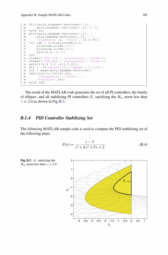
The result of the MATLAB code generates the set of all PI controllers, the familyof ellipses, and all stabilizing PI controllers Sγ satisfying the H∞ norm less thanγ = 2.0 as shown in Fig.B.3.

B.1.4 PID Controller Stabilizing Set

The following MATLAB sample code is used to compute the PID stabilizing set ofthe following plant:

P(s) = s − 3

s3 + 4 s2 + 5 s + 2. (B.4)

Fig. B.3 Sγ satisfying theH∞ norm less than γ = 2.0

-4 -3.5 -3 -2.5 -2 -1.5 -1 -0.5 0 0.5 1

-4

-3

-2

-1

0

1

2


1 % PID stabilizing set2 clear all;3 syms s;4 kp = sym('kp','real');5 ki = sym('ki','real');6 kd = sym('kd','real');7 w = sym('w','real');8 N = [1 -3]; % Numerator9 D = [1 4 5 2]; % Denominator10 tam_N = size(N);11 tam_D = size(D);12 n = tam_D (2) -1;13 m = tam_N (2) -1;14 ze = roots(N); % Zeros of N(s)15 l = 1;16 nz = 0;17 for k = 1:m18 if real(ze(k)) > 019 nz = l; % RHP Zeros of N(s)20 l = l + 1;21 end22 end23 signature = n - m + 1 + 2*nz; % Signature number24 D_s = poly2sym(D,s); % D(s)25 N_s = poly2sym(N,s); % N(s)26 N_ms = subs(N_s , -s); % N(-s)27 Delta = s*D_s + (ki+kd*s^2)*N_s + kp*s*N_s; % ...

Characteristic equation28 Delta = collect(Delta ,s); % simplify expression in ...

terms of s29 V_s = collect(Delta*N_ms ,s); % V = Delta*N(-s)30 V = subs(V_s , 1i*w); % V(jw)31 Vr = real(V); % Real part of V32 Vi = imag(V); % Imaginary part of V33 for kp_f = -4:0.2:0.65 % Evaluate for a fixed Kp34 f_kp = subs(Vi , kp , kp_f); % substitute value of Kp35 f_Vi = sym2poly(f_kp); % convert to polynomial36 r = roots(f_Vi); % find the roots37 tam3 = size(r);38 l = 1;39 r2 = 0;40 for k = 1:tam341 if imag(r(k)) == 0 && real(r(k)) > 0 % select ...

real , positive roots42 r2(l) = real(r(k));43 l = l + 1;44 end45 end46 wt = [0 r2(2) r2(1)] ;47 tam_w = size(wt);48 R(1) = subs(Vr , w, wt(1));49 C1(1,:) = [0,coeffs(R(1)), 0];50 Te(1,:) = [0,ki ,0];51 R(tam_w (2)) = subs(Vr, w, wt(tam_w (2)));52 for k=2: tam_w (2)53 R(k) = subs(Vr , w, wt(k));54 [C1(k,:),Te(k,:)] = coeffs(R(k));55 end56 C1 = double(C1);57 A = -[C1(1,1) C1(1,2) 0;-C1(2,1) -C1(2,2) 0;C1(3,1) ...

C1(3,2) 0]; % [kd ki kp]58 b = -[-C1(1,3);C1(2,3);-C1(3,3)];59 lb = [-300,-300,kp_f];60 ub = [300,300, kp_f];61 plotregion(A,b,lb ,ub,'y');62 hold on;


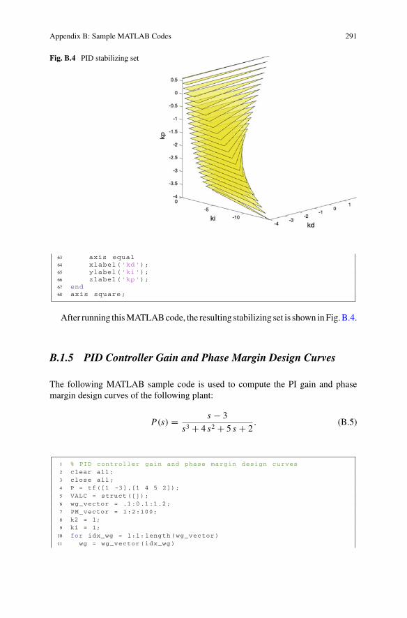
Fig. B.4 PID stabilizing set

63 axis equal64 xlabel('kd');65 ylabel('ki');66 zlabel('kp');67 end68 axis square;


B.1.5 PID Controller Gain and Phase Margin Design Curves

The following MATLAB sample code is used to compute the PI gain and phasemargin design curves of the following plant:

P(s) = s − 3

s3 + 4 s2 + 5 s + 2. (B.5)

1 % PID controller gain and phase margin design curves2 clear all;3 close all;4 P = tf([1 -3],[1 4 5 2]);5 VALC = struct ([]);6 wg_vector = .1:0.1:1.2;7 PM_vector = 1:2:100;8 k2 = 1;9 k1 = 1;10 for idx_wg = 1:1: length(wg_vector)11 wg = wg_vector(idx_wg)


12 k1 = 1;13 k2 = 1;14 for idx_PM = 1:1: length(PM_vector)15 k1 = 1;16 k4 = 1;17 PM = PM_vector(idx_PM)18 [MP ,PP] = bode(P,wg);19 phi = pi + PM*pi/180 - PP*pi /180;20 M2 = 1/(MP^2);21 Kp1 = sqrt(M2/(1+ tan(phi)^2));22 [A1 ,b1] = pid_set_continuous (Kp1);23 if (¬(isempty(A1)))24 for x = -6:0.1:625 Ki = x*wg^2 - wg*tan(phi)*Kp1;26 C = tf([x,Kp1 ,Ki],[1 0]);27 STA = isstable(feedback(C*P,1));28 if STA == 129 VALC{idx_PM ,idx_wg }(k1 ,:) = [x,Ki ,Kp1 ,wg ,PM];30 k1 = k1 + 1;31 else32 VALC{idx_PM ,idx_wg }(k1 ,:) = [0,0,0,0,0];33 k1 = k1 + 1;34 end35 end36 tam = size(VALC{idx_PM ,idx_wg });37 for k3 = 1:tam (1)38 if VALC{idx_PM ,idx_wg }(k3 ,:) �= [0,0,0,0,0]39 C = tf([VALC{idx_PM ,idx_wg }(k3 ,1),...40 VALC{idx_PM ,idx_wg }(k3 ,3),...41 VALC{idx_PM ,idx_wg }(k3 ,2)],[1,0]);42 Result = allmargin(C*P);43 if abs(Result.PhaseMargin (1)-PM) > 244 else45 info_GMPM{idx_PM ,idx_wg }(k4 ,:) = ...

[Result.GainMargin (1),Result.PhaseMargin (1),...46 Result.PMFrequency (1),Result.Stable ];47 k4 = k4 + 1;48 end49 end50 end51 end52 Kp2 = -sqrt(M2/(1+ tan(phi)^2));53 [A2 ,b2] = pid_set_continuous (Kp2);54 if (¬(isempty(A2)))55 for x = -6:0.1:656 Ki = x*wg^2 - wg*tan(phi)*Kp2;57 C = tf([x,Kp2 ,Ki],[1 0]);58 STA = isstable(feedback(C*P,1));59 if STA == 160 VALC{idx_PM ,idx_wg }(k1 ,:) = [x,Ki ,Kp2 ,wg ,PM];61 k1 = k1 + 1;62 else63 VALC{idx_PM ,idx_wg }(k1 ,:) = [0,0,0,0,0];64 k1 = k1 + 1;65 end66 end67 tam = size(VALC{idx_PM ,idx_wg });68 for k3 = 1:tam (1)69 if VALC{idx_PM ,idx_wg }(k3 ,:) �= [0,0,0,0,0]70 C = tf([VALC{idx_PM ,idx_wg }(k3 ,1),...71 VALC{idx_PM ,idx_wg }(k3 ,3),...72 VALC{idx_PM ,idx_wg }(k3 ,2)],[1,0]);


73 Result = allmargin(C*P);74 if abs(Result.PhaseMargin (1)-PM) > 275 else76 info_GMPM{idx_PM ,idx_wg }(k4 ,:) = ...

[Result.GainMargin (1),Result.PhaseMargin (1),...77 Result.PMFrequency (1),Result.Stable ];78 k4 = k4 + 1;79 end80 end81 end82 end83 end84 end85 %% Plot of PID gain and phase margin design curves86 figure (1)87 colors = hsv(length(wg_vector));88 legendInfo=cell(length(wg_vector) ,1);89 H = gobjects(length(wg_vector) ,1);90 for idx_wg = 1:1: length(wg_vector)91 wg = wg_vector(idx_wg);92 for idx_PM = 1:1: length(PM_vector) -293 h = plot3(wg*ones(1,length(info_GMPM{idx_PM ,idx_wg}...94 (:,1))),info_GMPM{idx_PM ,idx_wg }(: ,2),...95 info_GMPM{idx_PM ,idx_wg }(: ,1),'-','LineWidth ',1.5);96 hold on;97 set(h,'Color ',colors(idx_wg ,:));98 if(isempty(legendInfo{idx_wg }))99 legendInfo{idx_wg} = ['w_g = ' ...

num2str(wg_vector(idx_wg))];100 H(idx_wg ,1)=h;101 end102 end103 end104 legend(H,legendInfo);105 set(gca ,'zscale ','log')106 axis ([0 1.2 0 100 1 40])107 grid on108 ylabel('Phase Margin (deg)');109 xlabel('\omega_g (rad/s)');110 zlabel('Gain Margin ');

The following code corresponds to the function “pid_set_continuous()” used inthe previous sample code.

1 function [A, b] = pid_set_continuous(Kp)2 syms s;3 kp = sym('kp','real');4 ki = sym('ki','real');5 kd = sym('kd','real');6 w = sym('w','real');7 if Kp < -4 || Kp > 0.658 A = [];9 b = [];10 else11 N = [1 -3];12 D = [1 4 5 2];13 tam_N = size(N);14 tam_D = size(D);


15 n = tam_D (2) -1;16 m = tam_N (2) -1;17 ze = roots(N);18 l = 1;19 nz = 0;20 for k = 1:m21 if real(ze(k)) > 022 nz = l;23 l = l + 1;24 end25 end26 signature = n - m + 1 + 2*nz;27 D_s = poly2sym(D,s);28 N_s = poly2sym(N,s);29 N_ms = subs(N_s , -s);30 Delta = s*D_s + (ki+kd*s^2)*N_s + kp*s*N_s;31 Delta = collect(Delta ,s);32 V_s = collect(Delta*N_ms ,s);33 V = subs(V_s , 1i*w);34 Vr = real(V);35 Vi = imag(V);36 for kp_f = Kp:0.2:Kp37 f_kp = subs(Vi , kp , kp_f);38 f_Vi = sym2poly(f_kp);39 r = roots(f_Vi);40 tam3 = size(r);41 l = 1;42 r2 = 0;43 for k = 1:tam344 if imag(r(k)) == 0 && real(r(k)) > 045 r2(l) = real(r(k));46 l = l + 1;47 end48 end49 wt = [0 r2(2) r2(1)] ;50 tam_w = size(wt);51 R(1) = subs(Vr , w, wt(1));52 C1(1,:) = [0,coeffs(R(1)), 0];53 Te(1,:) = [0,ki ,0];54 R(tam_w (2)) = subs(Vr , w, wt(tam_w (2)));55 for k=2: tam_w (2)56 R(k) = subs(Vr , w, wt(k));57 [C1(k,:),Te(k,:)] = coeffs(R(k));58 end59 C1 = double(C1);60 A = -[C1(1,1) C1(1,2) 0;-C1(2,1) ...

-C1(2,2) 0;C1(3,1) C1(3,2) 0];61 b = -[-C1(1,3);C1(2,3);-C1(3,3)];62 lb = [-300,-300,kp_f];63 ub = [300,300, kp_f];64 end65 end66 end


100

Phase Margin (deg)

50100

g (rad/s)

Gai

n M

argi

n 101

0 0.2 00.4 0.6 0.8 1 1.2

wg = 0.1

wg = 0.2

wg = 0.3

wg = 0.4

wg = 0.5

wg = 0.6

wg = 0.7

wg = 0.8

wg = 0.9

wg = 1

wg = 1.1

wg = 1.2

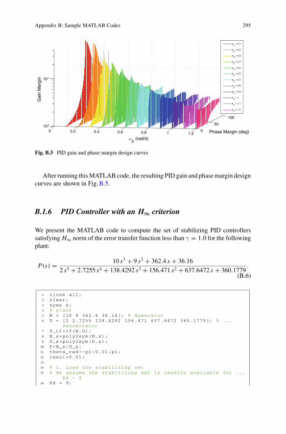
Fig. B.5 PID gain and phase margin design curves

After running thisMATLABcode, the resulting PID gain and phasemargin designcurves are shown in Fig.B.5.

B.1.6 PID Controller with an H∞ criterion

We present the MATLAB code to compute the set of stabilizing PID controllerssatisfying H∞ norm of the error transfer function less than γ = 1.0 for the followingplant:

P(s) = 10 s3 + 9 s2 + 362.4 s + 36.16

2 s5 + 2.7255 s4 + 138.4292 s3 + 156.471 s2 + 637.6472 s + 360.1779.

(B.6)

1 close all;2 clear;3 syms s;4 % plant5 N = [10 9 362.4 36.16]; % Numerator6 D = [2 2.7255 138 .4292 156 .471 637 .6472 360 .1779 ]; % ...

Denominator7 P_tf=tf(N,D);8 N_s=poly2sym(N,s);9 D_s=poly2sym(D,s);10 P=N_s/D_s;11 theta_rad=-pi:0.01:pi;12 resol =0.01;13

14 % 1. Load the stabilizing set15 % We assume the stabilizing set is readily available for ...

Kd = 916 Kd = 9;


17 load stab_pid_hinf_plant_00.mat;18 stabset = [Ki_data ,Kp_data ];19 poly_stabset = ...

simplify(polyshape(stabset ,'Simplify ',false));20 clear Ki_data Kp_data;21

22 % 2. Initial Sgamma is the stabilizing set23 poly_Sgamma = poly_stabset;24

25 % 3. Fix gamma and constructively determine S gamma set26 gamma =1.0;27 P_s = N_s/D_s;28 syms w 'real';29 P_jw= subs(P_s ,s,1i*w);30 P_r = simplify(real(P_jw));31 P_i = simplify(imag(P_jw)/w);32 P_mag2 = simplify(P_r*P_r + w*w*P_i*P_i);33

34 Ea2 = w^2/( gamma ^2* P_mag2);35 Eb2 = 1/( gamma ^2* P_mag2);36 Ec1 = -w^2*P_i/P_mag2;37 Ec2 = -P_r/P_mag2;38

39 w_freqs =[ linspace (1 ,20 ,800), linspace (1 ,20 ,800)];40 for idx = 1: numel(w_freqs)41 wr=w_freqs(idx);42 % (x - c1)^2 / a^2 + (y - c2)^2 / b^2 = 143 c1 = double(subs(Ec1 ,w,wr)) + wr*wr*Kd;44 c2 = double(subs(Ec2 ,w,wr));45 bb = double(subs(Eb2 ,w,wr));46 aa = double(subs(Ea2 ,w,wr));47 x=c1+sqrt(aa)*cos(theta_rad);48 y=c2+sqrt(bb)*sin(theta_rad);49

50 poly_Sgamma = ...subtract(poly_Sgamma ,polyshape(x,y,'Simplify ',true));

51 end52

53 % 4. Collect sample ellipses for display (optional)54 clear idx w_freqs;55 gamma =1;56 w_freqs=linspace (1 ,200 ,800);57 coords_x = NaN(numel(w_freqs),numel(theta_rad));58 coords_y = NaN(numel(w_freqs),numel(theta_rad));59 parfor idx = 1:numel(w_freqs)60 wr=w_freqs(idx);61 % (x - c1)^2 / a^2 + (y - c2)^2 / b^2 = 162 c1 = double(subs(Ec1 ,w,wr)) + wr*wr*Kd;63 c2 = double(subs(Ec2 ,w,wr));64 bb = double(subs(Eb2 ,w,wr));65 aa = double(subs(Ea2 ,w,wr));66 x=c1+sqrt(aa)*cos(theta_rad);67 y=c2+sqrt(bb)*sin(theta_rad);68

69 coords_x(idx ,:)=x;70 coords_y(idx ,:)=y;71 end72

73 figure;74 fill(poly_stabset.Vertices (:,1), ...75 poly_stabset.Vertices (:,2),'y');76 hold on;77 plot(poly_Sgamma.Vertices (:,1), ...78 poly_Sgamma.Vertices (:,2),'-',...79 'LineWidth ',2, 'Color ', [0 0 0]);80 for idx = 1:size(coords_x ,1)81 x=coords_x(idx ,:) ';


Fig. B.6 Sγ satisfying the H∞ norm less than γ = 1.0 with kd = 9

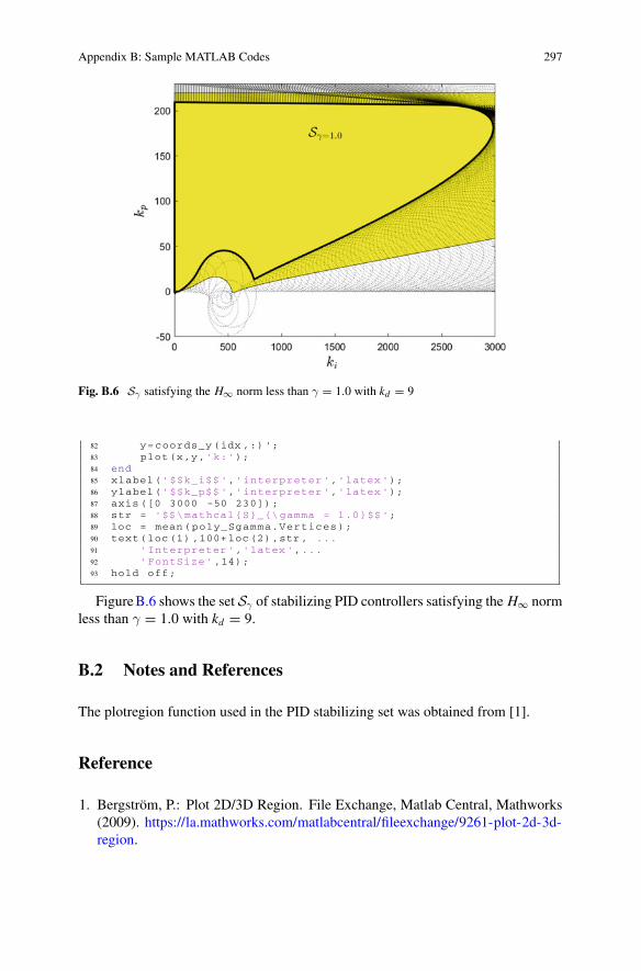
82 y=coords_y(idx ,:) ';83 plot(x,y,'k:');84 end85 xlabel('$$k_i$$ ','interpreter ','latex ');86 ylabel('$$k_p$$ ','interpreter ','latex ');87 axis ([0 3000 -50 230]);88 str = '$$\mathcal{S}_{\gamma = 1.0}$$';89 loc = mean(poly_Sgamma.Vertices);90 text(loc(1) ,100+loc(2),str , ...91 'Interpreter ','latex ',...92 'FontSize ' ,14);93 hold off;

FigureB.6 shows the set Sγ of stabilizing PID controllers satisfying the H∞ normless than γ = 1.0 with kd = 9.

B.2 Notes and References

The plotregion function used in the PID stabilizing set was obtained from [1].

Reference

1. Bergström, P.: Plot 2D/3D Region. File Exchange, Matlab Central, Mathworks(2009). https://la.mathworks.com/matlabcentral/fileexchange/9261-plot-2d-3d-region.

https://la.mathworks.com/matlabcentral/fileexchange/9261-plot-2d-3d-region

https://la.mathworks.com/matlabcentral/fileexchange/9261-plot-2d-3d-region

Index

SymbolsH∞, 29H∞ criterion, 287, 295H∞ norm, 24, 25, 27, 235, 236, 238, 252H∞ optimal, 249Sγ , 235, 239, 241–243, 246–248, 251, 255,

259, 260, 276, 278σ-Hurwitz, 63, 64, 261σ-signature, 64

AAC drives, 261, 280Achievable Gain–Phase Margin Design

Curves, 163, 167, 173, 177, 181, 187,205, 212, 266

Achievable performance, 178, 182, 189, 191,192, 195, 198, 227–229, 266, 268

Adaptive, 31Admissible range, 66Algebraic Riccati equation, 24Allowable range, 56, 60, 265Antiwindup, 30Automatic PID tuning, 30Axis-parallel ellipse, 240, 245, 254, 258–

260, 276

BBandwidth, 158, 162Black’s amplifier, 21Bode magnitude plot, 131Bode plot, 130, 139, 148, 149, 155–157

CCharacteristic equation, 15, 165, 220

Characteristic polynomial, 38, 50, 98, 99,226, 265, 270

Circle Cγ , 240Closed half-plane, 64Closed-loop system, 2, 4, 5, 13, 14, 17Cohen-Coon, 11, 16, 30Complex Hurwitz Signature, 129Complex root boundary, 73Constant gain, 44, 177, 193, 197, 224, 266,

267Constant gain stabilization, 47, 50, 52Constant magnitude, 155Constant phase, 159, 162, 177, 193, 197, 224Continuous-time systems, 29, 201Control engineering, 1, 71Control error, 20Control signal, 18, 20Control theory, 1, 20Convex set, 55, 59Coprime, 44, 73Critical point, 235, 242, 243, 255Cylinder, 161, 164, 178, 193, 197

DData-based design, 146Data-driven synthesis, 123Deadbeat control, 98Delay-free systems, 80, 84, 156Design curves, 283Desired performance, 9, 17, 208Diagonal controller matrix, 219Diagonalization, 217Diagonal polynomial matrix, 219Diagonal transfer function, 219Digital control, 97, 117, 120Digital controllers, 201


299

https://doi.org/10.1007/978-3-030-18228-1

300 Index

Digital PI, 201Digital PID controllers, 97, 98, 273, 275Discrete-time, 203, 251Discrete-time feedback control system, 98Discrete-time integrator, 98Discrete-time system, 112Disturbance rejection, 3, 30, 39Disturbances, 2, 24, 269–271Disturbance signal, 271, 272Dominant pole placement, 16, 30, 77, 274Dynamic observer, 20Dynamic systems, 1, 251

EEllipse, 159, 160, 162, 164, 181, 187, 190,

203, 210, 211, 289Ellipse Eγ(ω), 241Elliptical cylinder, 160, 186Error signal, 7, 17, 18, 37, 239, 270, 271Error transfer function, 30, 235, 236, 238,

241, 245, 247, 249, 251, 252, 275Even and odd decomposition, 44, 45, 54, 55,

58, 60

FFamily of ellipses, 242, 246, 259, 260, 276Feasible range, 113, 141, 143, 204, 212Feasible strings, 47, 49, 53Feedback, 2Final Value Theorem, 221First-order controllers, 72, 249First-order plant, 95Fragile, 21, 25, 26, 28Fragility, 21, 26, 29, 31Frequency response, 123, 124, 131, 156,

161, 185, 201, 208Full state feedback, 23

GGain and phase margins, 17, 31, 156, 222Gain crossover frequency, 17, 155, 156, 163,

217, 224, 227–229Gain margin, 17, 20, 29, 156, 205, 217, 218,

220, 222, 224, 225, 227, 229, 244,246

Gain–phase margin design, 205Gain–phase margin design curves, 156, 163,

164, 170, 174, 207, 224, 225, 285,291, 295

Geometric figures, 155Guaranteed gain margin, 237, 238, 243

Guaranteed phase margin, 237, 238, 243

HHalf-bridge voltage source inverter, 261, 263Harmonic, 270–272Hermite–Biehler theorem, 79Hermite–Biehler-type result, 98High-order controllers, 21, 26Hurwitz, 38, 44, 45, 47, 63, 64, 220Hurwitz Signature, 126

IIdentified analytical model, 123Identified model, 123Independent SISO loops, 217Industrial processes, 1Inputs, 2, 4, 24Integral absolute error, 17Integral action, 6, 19, 39Integral control, 3Integral square error, 17Integral time-weighted absolute error, 17Integrator, 3–5, 18, 19, 220, 247Interlacing conditions, 102, 103Internal model control, 13

JJury’s test, 109

LLaplace, 38, 269, 270Left half-plane, 24, 25, 41Linear inequalities, 65, 98, 119, 143Linear programming, 97, 98, 125Linear-Quadratic Regulator (LQR), 20, 21,

77Linear time-invariant systems, 79, 155Loci, 159, 162, 203, 210, 224Loop-shaping, 249Low-frequency band, 123

MMajor and minor axes, 240, 245, 246MATLAB, 283, 285, 287, 289, 291, 295Maximal delay tolerance, 120Maximally deadbeat control, 117Maximum achievable, 63–65, 67, 70MIMO controller, 217, 219MIMO plant, 217

Index 301

Minimum achievable, 242Model-based approach, 123Model-based design, 146Model-free approach, 123Monic polynomial, 63Multivariable, 231Multivariable controller, 29, 217, 222, 231Multivariable plant, 224Multivariable stability margins, 222Multivariable systems, 217

NNeimark’s D-decomposition, 72, 248Net change in phase, 41, 64Nichols charts, 155Nonlinear, 2, 18Nyquist plot, 17, 124, 139, 155, 255

OOddmultiplicities, 43, 46, 51, 52, 54, 56, 58,

60, 66, 67, 106, 107, 111, 115, 167,172, 177, 265

Open half-plane, 64Open-loop stable, 186, 191Open-loop stable plant, 80Open-loop system, 9, 11, 17Open-loop unstable, 188, 195Open-loop unstable plant, 80Optimal control, 20, 21Optimization, 21, 25, 31Outputs, 2, 24Overshoot, 247, 274, 278

PPadé approximation, 13, 262Parametrization, 27, 155, 158Perturbation matrix, 222Phase, 125, 126, 128, 129, 131–133, 139,

145, 149Phase crossover frequency, 17, 156Phase margin, 17, 20, 22, 23, 29, 156, 163,

222Phase unwrapping, 104, 108PI and PD controller, 274, 276, 282PI and PID controllers, 13, 14, 16, 17, 235,

239PI controller, 14, 54, 155, 201, 239, 242, 255,

287, 289PID controller, 6–8, 21, 29, 160, 208, 283,

295, 297PID stabilization, 79, 91

PID stabilizing set, 88, 91, 97, 114, 136, 164,177, 180, 194, 197, 199, 201

PI or PID controller, 14, 44, 235PI stabilizing set, 80, 81, 84, 110, 168, 173Pole placement, 14Pole-zero cancellation, 280Position control, 261Proper, 73, 114, 137, 156, 218, 220–222,

225, 236Proportional, 201

QQuasipolynomials, 79, 95

RRational, 38, 73, 246Rational function, 97–99, 103, 104, 109,

125, 128, 129Real polynomials, 100, 102, 103, 105Real rational function, 125, 144Real root boundary, 73Reference, 3, 262, 269–271Reference signal, 239Relative degree, 130, 131, 136, 145, 220, 221Relay feedback, 30Resonant controller, 62Right half-plane, 29, 41Robustness, 3, 20–22, 26, 29, 235, 246–248Robust stability, 5Root clustering, 100, 102, 119Root counting, 40, 97, 98, 100, 104, 105, 109Root distribution, 104Root invariant region, 72, 74, 146, 179, 181Rotating dq frame, 262Routh–Hurwitz criterion, 39

SSampling period, 97, 108, 117, 201, 208Schur stability, 97–99, 102, 103Schur stable, 98Servomechanisms, 3Setpoint, 18Settling time, 69, 247, 274, 278Signature, 41, 43, 46, 55, 56, 76, 125, 126,

128, 129, 135, 146, 148, 242Signature formulas, 40, 44, 60, 97, 167, 172,

177, 265Signature-invariant regions, 146Signature method, 246, 258Signature requirement, 54, 58–60, 62, 167,

172, 177, 265

302 Index

Simultaneous specifications, 155, 164, 173,178, 181, 188, 190, 194, 205

Single-input single-output, 217Sinusoidal signals, 270SISO loops, 217, 219, 220, 224Smith form, 218, 224Smith-McMillan, 217–219, 222, 224, 225,

231Smith-McMillan plants, 219, 225Stability, 58, 59, 84, 134, 145, 167, 172, 177,

220, 247, 265Stability margins, 39, 71, 235Stabilizing controllers, 47, 247, 271Stabilizing region, 117Stabilizing set, 38, 79, 136, 203, 211, 224,

225, 283, 285, 287, 289, 291, 297State feedback, 20, 21, 77Steady-state gain, 80, 87Step response, 9, 69, 170, 174, 208, 213, 278Straight line, 139, 146, 155, 159, 164, 165,

169, 173, 181, 187, 190, 203, 210,211

Strictly proper, 218, 236, 246Sweeping, 55, 57, 59, 61, 65, 67, 74, 76, 242,

260, 265, 278Synchronous machine, 261, 280System identification, 31, 274

TTchebyshev polynomials, 98, 100, 101, 110,

122Tchebyshev representation, 97, 98, 100, 103,

105, 107, 112, 203, 211Telescoping, 67, 69, 70, 242Time constant, 14, 19, 80, 87

Time-delay, 79, 80, 87, 185Time-delay tolerance, 163, 222Time response, 7, 8, 15, 16, 63, 247, 273Tracking, 3, 39, 218, 220, 261Tracking error, 98Transfer function matrix, 218Transient response, 6, 39, 247, 248Trial and error method, 8Two-input two-output system, 224

UUncertainty, 3Unimodular matrix, 220Unimodular polynomial matrices, 219, 221Unit circle, 97, 102, 112, 115, 116, 204, 211Unity feedback control loop, 63, 73, 241,

251, 255, 269

WWeighting function, 245Windup, 18

YYJBK parametrization, 124

ZZero steady-state error, 6, 247Ziegler–Nichols frequency response, 10Ziegler–Nichols plant, 79–89, 91, 93, 94,

186, 188, 191, 195Ziegler–Nichols step response, 9, 11

Documents

Analytical Design of PID Controllers - Springer Link