Poverty and FoodConsumption in

Urban Zaire

Hamid Tabatabai

OCTOBER 1993

WORKING PAPER 47

CORNELL FOOD AND NUTRITION POLICY PROGRAM

POVERTY AND FOOD CONSUMPTION IN URBAN ZAIRE

Hamid Tabatabai*

* The author is a senior economist at the International Labour Office,Po1i ci es and Programmes for Development Branch, Employment and DevelopmentDepartment, Geneva.

The Cornell Food and Nutrition Policy Program (CFNPP) was created in 1988 withinthe Division of Nutritional Sciences, College of Human Ecology, CornellUniversity, to undertake research, training, and technical assistance in food andnutrition policy with emphasis on developing countries.

CFNPP is served by an advisory committee of faculty from the Division ofNutritional Sciences, College of Human Ecology; the Departments of AgriculturalEconomics, Nutrition, City and Regional Planning, Rural Sociology; and from theCornell Institute for International Food, Agriculture and Development. Graduatestudents and faculty from these units sometimes coll aborate with CFNPP onspecific projects. The CFNPP professional staff includes nutritionists,economists, and anthropologists.

CFNPP is funded by several donors including the Agency for InternationalDevelopment, the World Bank, UNICEF, the United States Department of Agriculture,the New York State Department of Health, The Thrasher Research Fund, andindividual country governments.

Preparation of this document was financed by the U.S. Agency for InternationalDevelopment under USAID Cooperative Agreement AFR-000-A-0-8045-00.

For information about ordering this manuscript and other working papers in theseries contact:

This Working Paper series provides a vehicle for rapid and informal reporting ofresults from CFNPP research. Some of the findings may be preliminary and subjectto further analysis.

This document was word processed and formatted by Gaudencio Dizon. Themanuscri pt was ed ited by El izabeth Mercado. The cover was produced by BrentBeckley.

ISBN 1-56401-147-X~ 1993 Cornell Food and Nutrition Policy Program

CFNPP Publications Department315 Savage Hall

Cornell UniversityIthaca, NY 14853

607-255-8093

CONTENTS

LIST OF TABLES

LIST OF FIGURES

LIST OF ABBREVIATIONS

ACKNOWLEDGEMENTS

FOREWORD

1. INTRODUCTION

2. REVIEW OF THE LITERATURE

General BackgroundPoverty, Food Consumption, and Nutrition

Sources of Empirical InformationThe Evolution of Consumption Expenditures in KinshasaFood Consumption and Nutritional Status

3. DATA AND METHODOLOGY

The SurveysThe Methodology

Poverty LinePoverty Indices and Profiles

4. POVERTY AND FOOD CONSUMPTION: A PRELIMINARY ANALYSIS

Household Size in "Consumption Units"Calorie "Consumption"The Choice of RDAHousehold Demographic and Socioeconomic Characteristics

Demographic Characteristics of Households byExpenditure Category

Socioeconomic Characteristics of Households byExpenditure Category

v

vii

viii

ix

x

1

3

3666

10

14

14161719

22

22243235

35

37·

5. POVERTY PROFILES 42

Determination of Poverty Lines 42Poverty Incidence 44Poverty Profiles 47Multivariate Analysis 50Extent of Inequality 52

6. CONCLUSIONS 57

APPENDIX - AXIOMATIC APPROACH TO THE CONSTRUCTION OF POVERTYINDICES: A REVIEW

REFERENCES

-iv-

59

64

1

2

3

4

5

6

7

8

9

10

11

12

LIST OF TABLES

Socioeconomic and Human Welfare Indicators

Kinshasa: Evolution of Consumption Expenditures, 1969,1975 and 1986

Kinshasa: Consumption of Food Commodities, 1969, 1975,and 1986

Kinshasa and Bandundu Town: Distribution of Samplesby "Strate"

Alternative Sets of Conversion Coefficients for theCalculation of Household Size in Consumption Units

Kinshasa and Bandundu Town: Frequency Distributionof Calories for Sample Households

Kinshasa and Bandundu Town: Comparison of Full andRestricted Samples

Kinshasa and Bandundu Town: Demographic Indicatorsby Monthly Consumption Expenditures per ConsumptionUnit Category .

Kinshasa and Bandundu Town: Distribution of Householdsby Monthly Consumption Expenditures per ConsumptionUnit and "Strate"

Kinshasa and Bandundu Town: Distribution of Householdsby Monthly Consumption Expenditures per Consumption Unitand Socio-Professional Category of the Household Head

Kinshasa and Bandundu Town: Level and Structure ofExpenditures by Monthly Consumption Expendituresper Consumption Unit

Kinshasa and Bandundu Town: Alternative Specificationsof Calorie Cost Function

-v-

5

9

11

15

23

28

33

36

38

40

41

43

13

14

15

16

17

18

Kinshasa and Bandundu Town: Poverty Lines and Incidence

Kinshasa: Decompositions of Poverty (Medium Poverty Line)

Bandundu Town: Decompositions of Poverty(Medium Poverty Line)

Kinshasa and Bandundu Town: Typical Results ofMultivariate Analysis

Kinshasa and Bandundu Town: Do Female-Headed HouseholdsSpend Money "Better?"

Kinshasa: Distribution of Expenditures Among ExpenditureGroups, 1969 and 1986

45

48

49

51

53

54

19 Kinshasa and Bandundu Town: Gini Coefficients of ExpenditureDistribution 56

-vi-

la

lb

2

LIST OF FIGURES

Alternative Sets of Conversion Coefficients: Males

Alternative Sets of Conversion Coefficients: Females

Kinshasa and Bandundu Town: Frequency Distributionof Calories per Consumption Unit per Day

-vii-

25

26

29

CEPLANUT

CU

INS

MCE

RDA

LIST OF ABBREVIATIONS

Centre de Planification Nutritionelle

consumption unit

Institut National de la Statistique

monthly consumption expenditures

recommended dietary allowance

-viii-

ACKNOWLEDGEMENTS

This study would not have been possible without the kind assistance of theInstitut National de la Statistique (INS), Kinshasa, which provided the relevantdata from the 1985/86 household surveys of Kinshasa and Bandundu Town. Some ofthe key variables used in the study were constructed by the INS at author'srequest. My thanks go in particular to Messrs. Kayembe Lunganga, Lukaku Nzinga,Kasongo Mbaya, and Kubindikila Kalenga for their help at crucial moments.

Many useful discussions were held at various stages with other researchersinvolved in the larger Cornell project on Zaire. I would especially like tothank Prof. Erik Thorbecke, the principal investigator of the project, Mr. waBilenga Tshishimbi, its coordinator, and Dr. Blane Lewis of Cornell University;Dr. Glenn Rogers of the USAID, Kinshasa; Prof. Jef Maton of the University ofGent; and Prof. Kalonji Ntalaja of the University of Kinshasa for sharing withme their knowledge of Zaire as well as their own'findings in the course of theproject. I am also grateful for the comments of David Sahn of CFNPP and PeterPeek, Jean Majeres, and Steve Miller of the ILO on an earlier draft. Responsi­bility for any errors rests solely with the author.

-ix-

FOREWORD

Zaire is one of the most resource rich countries in sub-Saharan Africa, andtherefore, perhaps is the best illustration of the failure of state interventionin the economy, as manifested by economic decline and great social hardship. Inaddition, Zaire stands out in terms of the failure to pursue and sustain anyserious effort at economic reform. Whatever start was made toward removing thedistortions that discriminated against small-scale agriculture and manufacturingduri ng the 1980s they were reversed, contri but i ng to the present pol it ica1,social and economic crisis that grips Zaire.

While the magnitude of Zaire's policy failures are greater than mostAfrican countries, there is nonetheless much to be learned by exploring not onlythe genesis of the crisis, but what are the appropriate adjustment policies toreverse the declining growth rates and deteriorating living standards. It is inthis context that Zaire, one of the most populous and well endowed countries inAfrica, is included in a multi-country research study of the Cornell Food andNutrition Policy Program (CFNPP), exploring the impact of economic reform ongrowth, income distribution, and poverty.

Each of the country studies undertaken by CFNPP involve a combination ofanalytical approaches. These include a descriptive analysis of the evolution ofpolicy, and complete understanding of the structure of the economy, including thefunctioning of markets and incentive structures. This provides a basis forunderstanding the contribution of structure, pol icy and external factors toeconomic performance and living standards. Such an effort for Zaire is found inCFNPP Monograph 16, by wa Bilenga Tshishimbi and Peter Glick. Asecond componentof the research strategy involved a thorough analysis of the characteristics ofpoverty. In particular, the concern is identifying the incidence of poverty, andprofiling who the poor are, including understanding issues such as thecontribution of education, the sector of employment and gender of household headto consumption and poverty. This Working Paper, prepared by Hamid Tabatabai,presents the findings of such an effort.

The third component of the research strategy involved bringing together thework on the functioning of the economy as a whole, including various factor andproduct markets, and the poverty profile, into a more formal analytic frameworkfor policy analysis. This is done for Zaire through the construction of a SocialAccounting Matrix, and a input-output model, as discussed in the companionWorking Paper 55, by Solomane Kon~ and Erik Thorbecke.

The research undertaken by CFNPP has been a collaborative effort. In thecase of Zaire, this has involved a large number of contributors to the project,from a number of Zairian and international institutions. Special note of theassistance of the Institut National de la Statistique (INS) in Kinshasa iswarranted. Furthermore, the author of this report, Hamid Tabatabai, while having

-x-

historical roots with Cornell University, is presently working at the Policiesand Programmes for Development Branch, Employment and Development Department,International Labour Office (ILO). This research is the result of acollaborative effort bewteen CFNPP and the ILO and was financed from a grantreceived by CFNPP from the Africa Bureau anf Zaire Mission of the U.S. Agency forInternational Development.

David SahnDirector/Cornell Food and Nutrition Policy Program

Samir RadwanChief/Policies and Programmes for Development Branch, Employment and DevelopmentDepartment, International Labour Organization

-xi-

I

1. INTRODUCTION

Zaire is the second largest sub-Saharan African country by area (after theSudan) and the third largest by population (after Nigeria and Ethiopia). Despiteimmense natural resources, its population is among the poorest in the region andin the world. Long beset with problems, the economy of Zaire has gone from badto worse, despite perennial efforts at stabilization with the cooperation ofinternational financial agencies. The changes in the exchange rate, to take aparticularly sensitive indicator, illustrate the dramatic loss of control overthe economy in recent years: in April 1990, the parallel market rate was 500zaires to one US dollar; by early 1993, a dollar could be exchanged for severalmillion zaires!

The deepening economic crisis and the patent failure of past attempts toconta in it have roots that go far deeper than the economi c sphere alone. 1

Whatever these roots may be, however, the most vulnerable victims of the crisisare the impoverished masses whose ranks have continued to swell in recent years.Their plight is of all the more concern as their abject poverty contrasts sosharply with the wealth of the country's natural resources and the ostentatiouslifestyles of its elite.

This study is concerned with certain dimensions of poverty in urban Zaire:the extent of the poverty, the ident i fi cat i on of the poor, and the factorsassociated with their poverty. As part of the larger Cornell project on Zaire,this study covers Kinshasa, the capital city, and Bandundu Town. The analysisis based mainly on data from two household surveys carried out by the InstitutNational de la Statistique in 1985/86.

The study is organized as follows. Section 2, which provides a selectivereview of the literature, begins by highlighting the salient features of theeconomy and the overall state of welfare of the population. The main emphasisin this section, however, is on an analytical review of the significant researchstudies now available relating to poverty, food consumption, and nutritionalstatus in Kinshasa. The three sections that follow constitute the core of thestudy. Sect i on 3 descri bes the survey data and the methodology used in theanalysis of poverty. Section 4 is concerned with the initial stages of theanalysis that involve the construction of key variables and the presentation ofsome descriptive preliminary results. Section 5 presents the poverty profilesof Kinshasa and Bandundu Town, which constitute the main results of the study.

Indeed the current economic crlS1S is accompanied by a profound politicalcrisis that is probably even more intractable.

-2-

Some additional results based on multivariate techniques are also reported inthis section as are some statistics of inequality in the distribution ofexpenditures. The final section offers the ma"in conclusions of the analysis.The appendix briefly reviews the axiomatic approach to the construction ofpoverty indices, several of which are used in the study.

2. REVIEW OF THE LITERATURE

This section presents some general background observations on the Zairiansocioeconomic situation before reviewing selected studies on poverty, foodconsumption, and nutrition. Given the scope of the study and the availableliterature, this review focuses primarily on Kinshasa, but relevant evidencerelating to the country as a whole, its rural and urban areas, and smaller towns,especially Bandundu Town, will also be noted as appropriate.

GENERAL BACKGROUND

With a per capita income estimated at US$ 220 in 1990, Zaire is one of thelowest-income countries in the world (UNDP 1993, p. 139). This estimate iswidely believed to be too low because of the inadequate coverage of subsistenceproduction and informal sector activities, both of which are pervasive. 2 A morecomprehensive accounting of the subsistence and informal sectors may raise theestimated per capita income by as much as 50 to 70 percent or more, as recentwork by the Institut National de 1a Statistique suggests (INS 1990).3 Even so,however, the country's level of poverty relative to other nations is unlikely tochange significantly: the underestimation of such activities is not specific toZaire, even if a case could be made that it is relatively larger in this countrythan in most other low-income countries. The economy of Zaire is a desperatelypoor economy.

One would not come away with this impression by observing the country'sresource base. Indeed, few countries can boast of equally immense mineral andagri cultura1 resources. The most important mi nera1s are copper, diamonds,cobalt, zinc, and oil. Many other minerals are found there as well, althoughmost of them are exploited only on a small scale. Mineral exports accounted, in1988, for about two-thirds of foreign exchange earnings of the country and morethan half of government revenues (Tshishimbi and Glick 1990, p. 13).

Agriculture is, of course, the dominant sector for employment, providingjobs to more than 70 percent of the economically active population in 1986-1989(UNDP 1992). But its growth rate per capita has been poor (-0.7 percent a yearduring the 1980s). Despite this anaemic growth, the sector's share in GOP

2 See, for example, MacGaffey (1983) and several other studies by hermentioned in World Bank (1989b).

3 According to one estimate, if informal and unrecorded activities are takeninto account, GOP per capita in 1987 was US$ 360 rather than the official figureof US$ 160 (World Bank, 1989b, p. i, citing Cour, n.d.).

-4-

actually rose from 20 percent in 1965 to 30 percent in 1990 because the economyperformed di sma11 y, with GDP per cap ita dec1in i ng at an average rate of 2.2percent over the same 25-year period (World Bank 1992, pp. 218 and 222). Natureis not to blame for any of this. The agricultural sector in Zaire enjoys naturaladvantages that would be the envy of many other sub-Saharan African countries.The popul at i on dens ity is low and about half of the 1and area is covered byforests. The climate is favorable and rainfall is always plentiful throughoutthe country. The northern and southern halves of the country, which is dividedin the mi ddl e by the equator, enjoy complementary weather patterns with awarm/cool cycle in the north coinciding with a cool/warm cycle in the south(Tshishimbi and Glick 1990). This complementarity has long been regarded as amajor stabilizing factor in ensuring food supplies throughout the year.Agricultural production pattern is dualistic: millions of subsistence farmerscoexist with a plantation sector that produces primarily industrial and exportcrops. The potential for producing hydroelectric power is virtually unrivaledin sub-Saharan Africa.

The modern manufacturing sector is relatively small and relies largely onforeign capital and managerial skills. It coexists with a pervasive informalsector, which is more often than not revealingly referred to as the "secondeconomy," the "underground economy," the "unrecorded economy," or the "paralleleconomy." The sector is notable both for its enormity and for its extensiverange of doubtful practices. It is a refuge sector that figures prominently inthe survival strategy of most Zairians.

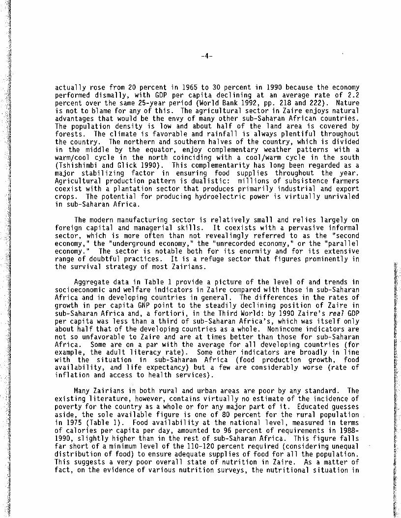
Aggregate data in Table 1 provide a picture of the level of and trends insocioeconomic and welfare indicators in Zaire compared with those in sub-SaharanAfrica and in developing countries in general. The differences in the rates ofgrowth in per capita GNP point to the steadily declining position of Zaire insub-Saharan Africa and, a fortiori, in the Third World: by 1990 Zaire's real GDPper capita was less than a third of sub-Saharan Africa's, which was itself onlyabout half that of the developing countries as a whole. Nonincome indicators arenot so unfavorable to Zaire and are at times better than those for sub-SaharanAfrica. Some are on a par with the average for all developing countries (forexample, the adult literacy rate). Some other indicators are broadly in linewith the situation in sub-Saharan Africa (food production growth, foodavailability, and life expectancy) but a few are considerably worse (rate ofinflation and access to health services).

Many Zairians in both rural and urban areas are poor by any standard. Theexisting literature, however, contains virtually no estimate of the incidence ofpoverty for the country as a whole or for any major part of it. Educated guessesaside, the sole available figure is one of 80 percent for the rural populationin 1975 (Table 1). Food availability at the national level, measured in termsof calories per capita per day, amounted to 96 percent of requirements in 1988­1990, slightly higher than in the rest of sub-Saharan Africa. This figure fallsfar short of a minimum level of the 110-120 percent required (considering unequaldistribution of food) to ensure adequate supplies of food for all the population.This suggests a very poor overall state of nutrition in Zaire. As a matter offact, on the evidence of various nutrition surveys, the nutritional situation in

-5-

Table 1 - Socioeconomic and Human Welfare Indicators

AllYear or Sub-Saharan Developing Tables

Indicator Period Zaire Africa Countries in Source

1. GNP per capita (US$) 1990 220 490 810 2, 51Average annual growth rate (%) 1965-80 -1.3 1.5 2.9 27, 51Average annual growth rate (%) 1980-90 -1.5 -1.1 2.5 27, 51

2. Real GDP per capita (PPP $) 1990 367 1,200 2,170 2, 51

3. Average annual rate ofinflation (%) 1980-90 60.9 22.3 27.9 27, 51

4. Food production per capita(1979-81 = 100) 1988-90 97 95 115 13, 51

5. Food availability(kcals per capita per day) 1988-90 2,130 2,250 2,490 13, 51

As percent of requirements 1988-90 96 93 107 13, 51

6. Life expectancy at birth (years) 1990 53.0 51.8 62.8 2, 51

7. Adul t 1i teracy rate (% 15+) 1990 72 47 65 5, 51Male 1990 84 58 75 5, 51Female 1990 61 36 55 5, 51

8. Percent of population withaccess to health services 1987-90 26 48 64 2

Urban 1987-90 40 80 90 10Rural 1987-90 17 36 49 10

9. Percent of population withaccess to safe water 1987-90 34 40 68 2

Urban 1987-90 59 65 82 10Rura 1 1987-90 17 28 60 10

10. Under-5 mortality rate (per1,000 live births) 1990 130 165 104 11 , 51

11. Infant mortality rate (per 1,000live births) 1991 96 103 71 11, 51

12. Incidence of poverty (%)Urban 1977-87 34 27 16Rural 1977-87 80' 61 35 16

• This actually refers to 1975; see World Bank (1988b).

Source: UNDP (1993), except for items 8 and 9 (UNDP 1992) and item 12 (UNDP 1990).

-6-

Zaire might be even worse than in the rest of sub-Saharan Africa (World Bank1989c, p. 12). The poorer state of access to health services (Table 1) may wellbe relevant in explaining this discrepancy.

POVERTY, FOOD CONSUMPTION, AND NUTRITION

This subsection reviews the findings of a few major studies on poverty, foodconsumption, and nutrition in order to set the stage for the detailed analysisthat follows. The available literature is overwhelmingly concerned withKinshasa.

Sources of Empirical Information

Detailed evidence on incomes and food consumption in urban areas isavailable in a series of studies by Joseph Houyoux and his collaborators thatreport the results of household budget surveys conducted in a number of cities.In the case of Kinshasa, time-series data are available from three householdbudget surveys carried out in 1969, 1975, and 1986. The INS also undertook arather ambitious set of surveys in 1985/86 covering Kinshasa and Bandundu Town,the two urban areas in the present study, and other cities. Some preliminaryresults of the analysis of INS surveys have been published (INS 1989a, 1989b).Adraft report by the World Bank (1989b) is the most comprehensive review to dateof poverty in Zaire, although it does not incorporate the results of the 1985/86INS surveys. Much of what follows in this review relies on the relevant materialassembled in the World Bank report but the original Houyoux studies and otherWorld Bank documents were also drawn upon as needed. This review is not merelydescriptive: the use of evidence and the interpretations provided here differ,at times, from those of the studies being reviewed, particularly in the case ofthe World Bank's poverty report. These differences will be pointed out asappropriate. Also, this review will not include the recently publishedpreliminary analysis of the INS survey data, as a full analysis of these datawill be presented in later sections of this study.

The Evolution of Consumption Expenditures in Kinshasa

Following a pilot survey in 1968 covering 60 households (Houyoux and Houyoux1970) a full-scale budget survey was conducted in Kinshasa in 1969 using astratified random sample of 1,471 African households (Houyoux 1973). This wasfollowed by a second full-scale survey in 1975 involving a similarly stratifiedrandom sample of 1,367 households. The third survey in the series in 1986(Houyoux 1987), however, was far more modest in both scale (only 205 households)and sampling technique. The latter survey sought to ensure roughly equal numbersof households in each of six expenditure categories, taking into account suchcharacteristics as the occupation and ethnic origin of the household head as wellas the zone of habitation).

-7-

The World Bank poverty report (1989b, hereafter called the Report) reliesheavily on the results of the first and third of these Kinshasa surveys,virtually ignoring the second one. The principal conclusions of the Report,which are essentially those arrived at by Houyoux himself (Houyoux 1973, 1987),are as follows (Report, pp. 27-30 and Annex I, pp. 3-9; see also World Bank1989a, pp. iii-iv):

(a) There is a positive relationship between household size and totalhousehold expenditure, and an inverse relationship between householdsize and expenditure per person.

(b) Average expenditure differentials between all income levels seem tohave narrowed from 1969 to 1986. The leveling-off between incomelevels is believed to arise from what Houyoux has referred to as thedua7isme culture7 of Kinshasa: the increase in economic level issystematically accompanied by an increase in obligations toward theextended family (whose poorer members will go to live with the better­off household, increasing its size and reducing the gap in expendituresbetween income levels).

(c) While the share of the food expenditure is inversely related to thelevel of income, the structure of expenditure (its division among food,housing, clothing, and miscellaneous items) remained the same for allincome levels.

(d) Most households surveyed in Kinshasa spend between 60 percent and 80percent of their total expenditure on food. (This was more or less thecase in 1969 but not in 1986).

(e) Expenditures over the 17 years separating the two surveys (1969-1986)kept pace with variations in the Kinshasa consumer price index.Despite food price increases, however, the average person consumed thesame quantity of food in Kinshasa in 1986 as in 1969 (about 17 kg permonth) .

(f) The Gini coefficients of per capita expenditure distribution areestimated to be 0.482 for 1969 and 0.490 for 1986. These estimates,which are based on grouped data from the Houyoux surveys, "indicate amoderately unequal size distribution of income in Kinshasa in 1969,becoming slightly more unequal in 1986" (Report, Annex I, p. 3). TheReport notes that "this trend can be explained by the opening up of theextended family and higher undeclared earnings" (ibid., fn 2).

(g) The pattern of food consumption changed somewhat (consumption of themain sources of vitamins and of the traditional sources of proteindecreased and consumption of bread, ri ce, and meat increased). Thechange has probably worsened the overall nutritional level of the poorwho cannot, for instance, replace fish with meat as an alternativesource of protein.

-8-

(h) Households headed by cadres or females had the highest per capitaconsumption expenditure and spent the lowest proportion of their incomeon food in both 1969 and 1986. By contrast, manual worker"s (bothsemiskilled and unskilled) and the unemployed appear to be worse off.

(i) Official wages in 1986 represented less than a third of reportedincome, wi th the 1argest share bei ng deri ved from i nforma1 sectoractivities. "Undeclared earnings" match official wages as a source ofincome.

The anal ys is in subsequent sections wi 11 provi de evi dence from the INSKi nshasa survey that bear on some of the above fi ndi ngs. A few of these,however, appear to be based on erroneous calculations or a misinterpretation ofthe evidence from the Houyoux surveys. These are discussed below.

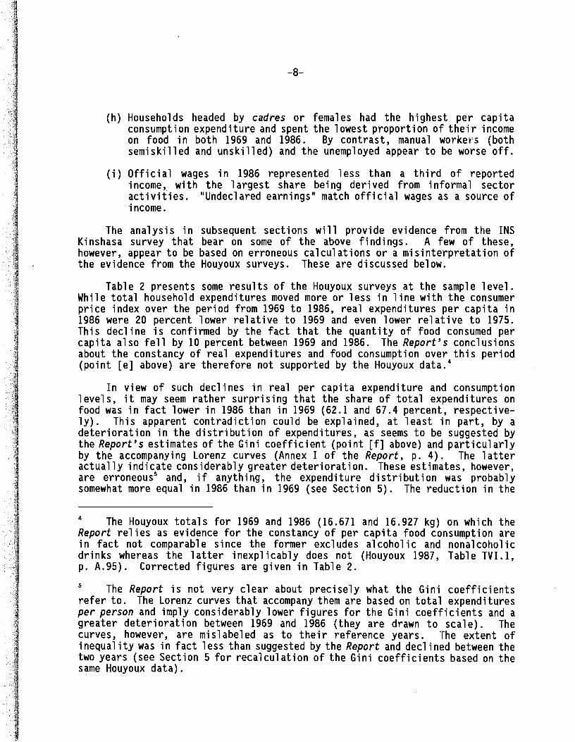
Table 2 presents some results of the Houyoux surveys at the sample level.While total household expenditures moved more or less in line with the consumerprice index over the period from 1969 to 1986, real expenditures per capita in1986 were 20 percent lower relative to 1969 and even lower relative to 1975.This decline is confirmed by the fact that the quantity of food consumed percapita also fell by 10 percent between 1969 and 1986. The Report's conclusionsabout the constancy of real expenditures and food consumption over this period(point [e] above) are therefore not supported by the Houyoux data. 4

In view of such declines in real per capita expenditure and consumptionlevels, it may seem rather surprising that the share of total expenditures onfood was in fact lower in 1986 than in 1969 (62.1 and 67.4 percent, respective­ly). This apparent contradiction could be explained, at least in part, by adeterioration in the distribution of expenditures, as seems to be suggested bythe Report's estimates of the Gini coefficient (point [f] above) and particularlyby the accompanyi ng Lorenz curves (Annex I of the Report, p. 4). The 1atteractually indicate considerably greater deterioration. These estimates, however,are erroneous5 and, if anything, the expenditure distribution was probablysomewhat more equal in 1986 than in 1969 (see Section 5). The reduction in the

4 The Houyoux totals for 1969 and 1986 (16.671 and 16.927 kg) on which theReport relies as evidence for the constancy of per capita food consumption arein fact not comparable since the former excludes alcoholic and nonalcoholicdrinks whereas the latter inexplicably does not (Houyoux 1987, Table TVI.l,p. A.95). Corrected figures are given in Table 2.

5 The Report is not very clear about precisely what the Gini coefficientsrefer to. The Lorenz curves that accompany them are based on total expendituresper person and imply considerably lower figures for the Gini coefficients and agreater deteri orat i on between 1969 and 1986 (they are drawn to scale). Thecurves, however, are mislabeled as to their reference years. The extent ofinequality was in fact less than suggested by the Report and declined between thetwo years (see Section 5 for recalculation of the Gini coefficients based on thesame Houyoux data).

-9-

Table 2 - Kinshasa: Evolution of Consumption Expenditures, 1969, 1975, and 1986

1969 1975 1986

Average expenditure per household (current zaires/month)Average expenditure per household (1969 = 100)

Consumer price index

Real average expenditure per household (1969 = 100)Real average expenditure per capita (1969 = 100)

Food consumption per capita (kg per month) (ex. beverages)

Percent share in consumption expendituresFoodHousingClothingMiscellaneous

Elasticity of expendituresFoodHousingClothingMiscellaneous

Number of sample householdsAverage number of members per household

• Refers to January-June." Refers to May.

31.42100

100

100100

16.671

100.067.414.97.3

10.4

0.781.211.532.33

1,4175.9

79.59253

244"

104105

16.051

100.059.615.99.3

15.2

1,3675.8

8,56327,253

27,701"

9880

15.048

100.062.115.84.7

17.4

0.621. 021. 872.55

2057.3

Source: Houyoux (1987), Tables TIl .3, p. A.44, TII.4, p. 45, and TVI.l, p. A.95.

-10-

food share in 1986 relative to 1969 is almost certainly due to the overrepresent­ation of the richer households in Houyoux's much smaller 1986 sample.

When incomes decline, the incidence of poverty will generally rise if theincome distribution remains the same or becomes more skewed. It may also risewhen income distribution improves (inequality declines) but not sufficiently.6As was argued above, per capita expenditures in Kinshasa were significantly lowerin 1986 than in 1969 and 1975. Expenditure distribution, however, was probablysomewhat more equal in 1986 than in 1969, as shown later in Section 5. The neteffect on poverty is therefore difficult to establish although, in view of themagnitudes involved, it probably increased.

Houyoux does not try to estimate the incidence of poverty in Kinshasa in anyof his studies even though his three surveys provided enough data to do so. TheReport takes a small step in this direction by adopting the simple method ofusing the "food adequacy standard" as a proxy, i.e., the fraction of householdbudget spent on food. It defines those spending 70 percent or more of theirexpenditures on food as poor and those spending 80 percent or more as ultrapoor(p. 28). This approach, however, is not taken to its logical conclusion toestimate the incidence of poverty or of ultrapoverty. It nevertheless permittedthe ident ifi cat ion of household categori es that were worse off. The Reportidentifies these, for 1986, as manual workers (semiskilled and unskilled) and theunemployed. An analysis of the 1985/86 INS data, however, suggests that thedispersion of expenditures within individual occupational groups is large andpoverty groups cannot easily be identified by reference to a single characteris­tic (see below).

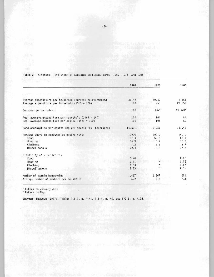
Food Consumption and Nutritional Status

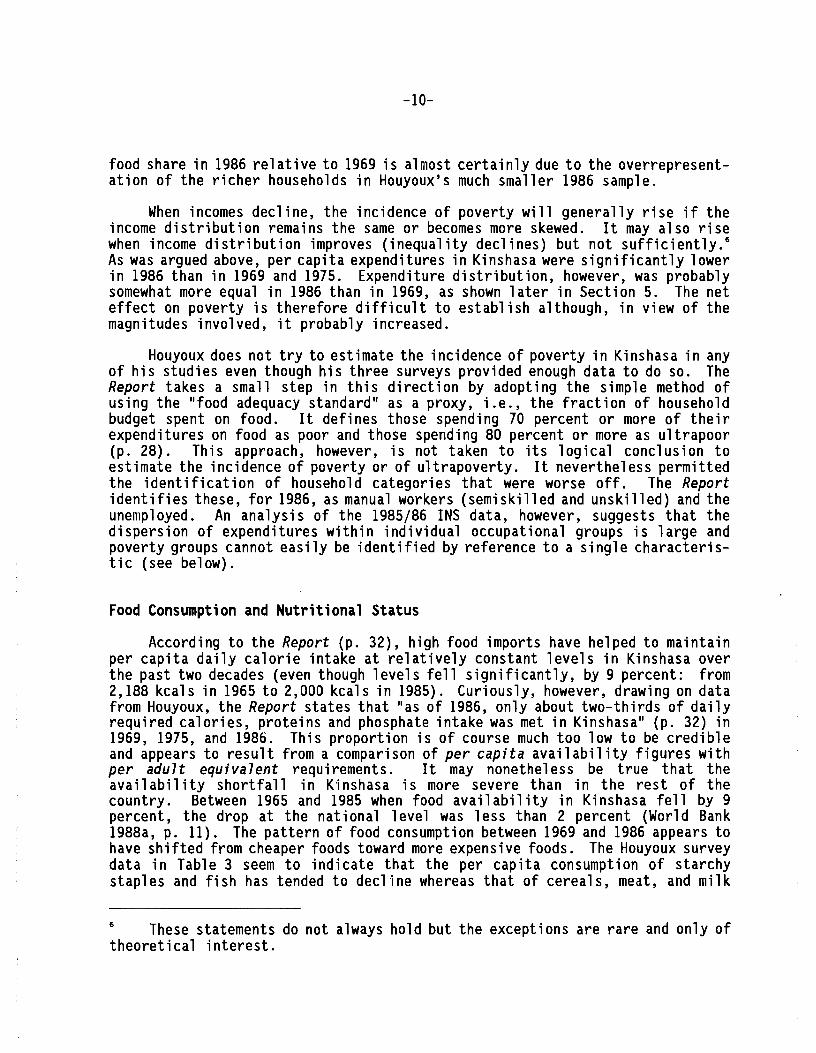
According to the Report (p. 32), high food imports have helped to maintainper capita daily calorie intake at relatively constant levels in Kinshasa overthe past two decades (even though levels fell significantly, by 9 percent: from2,188 kcals in 1965 to 2,000 kcals in 1985). Curiously, however, drawing on datafrom Houyoux, the Report states that "as of 1986, only about two-thirds of dailyrequired calories, proteins and phosphate intake was met in Kinshasa" (p. 32) in1969, 1975, and 1986. This proportion is of course much too low to be credibleand appears to result from a comparison of per capita availability figures withper adult equivalent requirements. It may nonetheless be true that theavailability shortfall in K"inshasa is more severe than in the rest of thecountry. Between 1965 and 1985 when food availability in Kinshasa fell by 9percent, the drop at the national level was less than 2 percent (World Bank1988a, p. 11). The pattern of food consumption between 1969 and 1986 appears tohave shifted from cheaper foods toward more expensive foods. The Houyoux surveydata in Table 3 seem to indicate that the per capita consumption of starchystaples and fish has tended to decline whereas that of cereals, meat, and mi"lk

6 These statements do not always hold but the exceptions are rare and only oftheoretical interest.

-]1-

Table 3 - Kinshasa: Consumption of Food Commodity, 1969, 1975, and 1986

Food Commodity Group 1969 1975

(Kilo per person per month)

1986

Cereals 2.644 2.342 2.990

Starchy staples 6.604 5.890 5.096

Sugar 0.351 0.496 0.437

Leguminous plants 0.635 0.652 0.510

Nuts (noix) 0.014 0.160 0.038

Vegetables (legumes) 2.715 2.394 2.412

Fruits 0.630 0.488 0.265

Fish 1. 418 1.305 1.058

Condiments 0.171 0.284 0.339

Meat 0.726 0.801 0.819

Alcoholic beverages 1.904 3.699 1.535

Milk 0.143 0.143 0.236

Oils 0.620 1.096 0.848

Nonalcoholic beverages 0.426 0.791 0.344

Total (excluding alcohol ic andnonalcoholic beverages)

Source: Houyoux (1986, p. 9).

16.671 16.051 15.048

-12-

has tended to rise. In a period of declining incomes and food consumption (seeTable 2), such a shift would imply a significant deterioration in incomedistribution, which is unlikely (see above and Section 5). Once again, it isprobably the overrepresentation of the richer households in the Houyoux's small1986 sample that accounts for this apparent shift. Maton (1992) in fact arguesconvincingly that the shift was in the opposite direction. Maton suggests thatas incomes declined, cassava has increased in importance as a source of caloriesin the diet of the Zairians, particularly in that of the poor. He estimates thatcassava accounts for about 45 percent of calories consumed in the country, aswell as in Kinshasa, and that this share exceeds 55 percent for the poor (Maton1992, p. 32). The increasing reliance on cassava as a cheap source of calorieshas been taking place in the context of a gradual decline in average availabilityof calories in the country since the mid-1970s (Maton 1992, p. 8).

Concerning nutritional status, available indicators point to a major problemof malnutrition throughout Zaire. A 1975 national sample survey coveringchildren below seven years of age indicated that 4.8 percent were wasted (acutelymalnourished, defined as weight-for-height lower than 2 standard deviations belowthe median), 44.8 percent were stunted (chronically malnourished, as evidencedby height-for-age less than 2 standard deviations below the median) and 28.8percent showed low weight-for-age (less than 2 standard deviations below themedian) (WHO 1989, p. 28). Current national estimates suggest that a quarter ofall young children are undernourished, although local surveys have often yieldedeven higher rates (World Bank 1989c, p. 11).

The evidence at subnational levels points to a wide regional variation andgenerally higher rates of malnutrition in rural than in urban areas (Report,pp. 33-34). In Kinshasa, however, rates are often as high as or higher than inrural areas (World Bank 1989c, p. 11). In the poorest parts of Kinshasa'sextension areas, such as Kimbanseke, the prevalence of malnutrition has beenfound to approach 70 percent. Nutritional surveys in Kinshasa indicated that in1986, 47.7 percent of children (up to five years of age) were mildly malnour­ished, 12.7 percent were moderately malnourished, and 2.3 percent suffered fromsevere malnutrition (Kalisa 1989, as cited 'in Kalonji et al. 1991, p.33).Another study reports that a Centre de Planification Nutritionelle's (CEPLANUT)survey in the same year revealed that about 30 percent of children in Kinshasawere chronically malnourished, with a height-for-age below two standarddeviations of WHO norms (Drosin 1988, as cited in Kalonji et al. 1991, p. 37).Comparable time-series data on nutritional indicators are not readily available,but indirect evidence suggests a strong likelihood of a deterioration in recentyears (declines in incomes and food consumption as discussed earlier).

While in the rural areas covered by "Health Zones" the prevalence ofmalnutrition does not in general exceed 20-25 percent, it can be as high as 60percent in areas outside of Health Zones. Various surveys in rural Bandundu havearrived at estimates of around 16 percent for the prevalence of low weight-for­age in the mi d-1980s (WHO 1989, p. 30) and more than 36 percent for theprevalence of chronic malnutrition (height-for-age below 90 percent ofinternational norm), again in the mid-1980s (Report, p. 34). In an interestingprel"iminary analysis of the pattern of differences over time and across

-13-

localities in the prevalence of malnutrition in the Kwilu, Bandundu, and itsproximate causes, Rogers (1990) distinguishes among three types of factors thatdetermine the prevalence: cyclical (including seasonal), transitional, andchronic. Based on available evidence from five health zones in the Kwilu, hearrives at a tentative breakdown of their respective contributions, whichhighlights the extreme volatility of rural malnutrition and its underlyingfactors. His evidence suggests that malnutrition could be significantly reducedif adaptive mechanisms were built into existing development activities. Forexample, primary health care needs to be complemented by greater efforts in theareas of family planning and nutrition education to increase child survivalrates. Similarly, in addition to improved transport infrastructure thatincreases access to markets, farmers may require assistance in boostingproduction to adapt more quickly to the new marketing opportunities.

3. DATA AND METHODOLOGY

The analysis in this study relies mainly on data from two household surveyscarried out in Kinshasa and Bandundu Town by the INS in 1985/86. 7 These surveysprovide, for the first time, fairly comprehensive data on sufficiently largesamples of households in these cities to permit a reasonably detailed analysisof poverty, expenditures, and food consumption. This section describes thesesurveys and the methods used in the ensuing analysis of poverty.

THE SURVEYS

The INS surveys of Kinshasa and Bandundu Town follow essentially the samemethodological approach. The description below relates ma"inly to the K"inshasasurvey, but the distinguishing features of the Bandundu survey will also be notedbri efly. 8

The sampling unit is a parcelle, which is a built-up piece of land that wasinhabited at the time of the survey in 1985/86. Most parcelles comprise a singlehousehold, but some may be inhabited by two or more households. There were atotal of 214,579 parcelles in the survey area, which encompassed the 22 of the24 zones of Kinshasa that have the characteristics of urban areas. These zoneswere grouped into five strata:

1. Residential: Gombe, Ngaliema, and Limete;2. Old neighborhoods: Kinshasa,Barumbu, Lingwala, and Kintambo;3. New developments: Ngiri-Ngiri and Kasa-Vubu;4. Planned developments: Bandalungwa, Kalamu, Lemba, Metete, and Ndjili);

and5. Extension areas: Mont-Ngafula, Selembao, Bumbu, Makala, Ngaba, Kisenso,

Masina, and Kimbanseke.

Within each of the five strata, the sampling ratio was set at 1/200. The sampletherefore consisted of 1,073 parcelles, of which 1,027 could be surveyed. Therewere 1,290 households in the surveyed parcelles, but comprehensive data could beobtained from only 83.7 percent of them, i.e., 1,080 households. The nonresponserate tended to be higher in the better-off strata. Details are given in Table 4.

The Kinshasa survey was unique among the urban surveys carried out in Zairein that the data were collected in four successive rounds over a full calendar

7

8

These surveys were part of a series covering several other cities as well.

For details on how the surveys were conducted, see INS (1984).

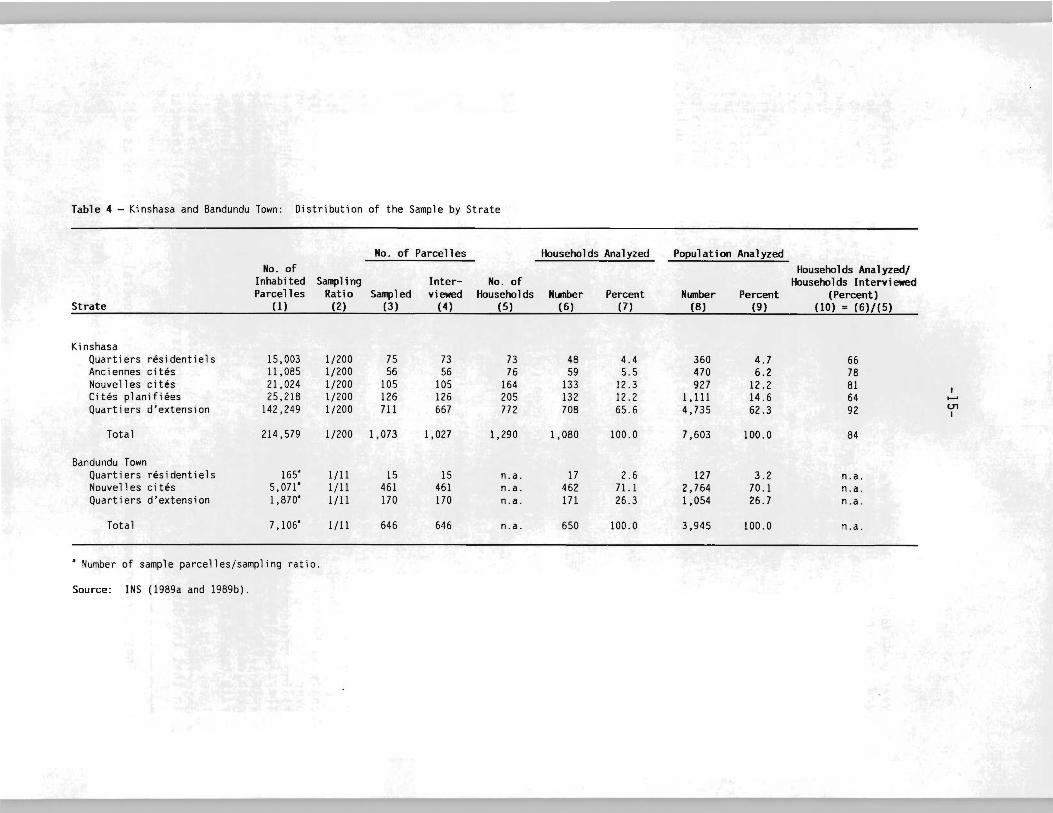
Table 4 - Kinshasa and Bandundu Town: Distribution of the Sample by Strate

No. of Parcelles Households Analyzed Population AnalyzedNo. of Households Analyzed/

Inhabited Sampling Inter- No. of Households InterviewedParcelles Ratio Sampled viewed Households N..mer Percent Ntnber Percent (Percent)

Strate (1) (2) (3) (4) (5) (6) (7) (8) (9) (10) = (6){(5)

KinshasaQuartiers residentiels 15,003 1/200 75 73 73 48 4.4 360 4.7 66Anciennes cites 11 ,085 1/200 56 56 76 59 5.5 470 6.2 78Nouve11 es ci tes 21,024 1/200 105 105 164 133 12.3 927 12.2 81 ICites planifiees 25,218 1/200 126 126 205 132 12.2 1,111 14.6 64 ......Quartiers d'extension 142,249 1/200 711 667 772 708 65.6 4,735 62.3 92 U"I

I

Total 214,579 1/200 1,073 1,027 1,290 1,080 100.0 7,603 100.0 84

Bandundu TownQuartiers residentiels 165' 1/11 15 15 n.a. 17 2.6 127 3.2 n.a.Nouvelles cites 5,071' 1/11 461 461 n.a. 462 71.1 2,764 70.1 n.a.Quartiers d'extension 1,870' 1/11 170 170 n.a. 171 26.3 1,054 26.7 n.a.

Total 7,106' 1/11 646 646 n.a. 650 100.0 3,945 100.0 n.a.

, Number of sample parcelles/sampling ratio.

Source: INS (1989a and 1989b).

-16-

year (February 1985 to February 1986). The average data for the year, therefore,are free from the i nfl uence of seasonal factors (a lthough seasonal ity is notoften a problem in a large city). The survey used two types of questionnaires.A demographic questionnaire gathered data on household size and composition andthe occupational characteristics of the household head (sector of activity, typeof employment, etc.), among other variables. A budget questionnaire in turncollected data, in four sections, on: (a) revenues (wages and salaries, netincome from self-employment, capital income, and other regular and irregularsources of income); (b) nonconsumption expenditures (purchases for the familyenterprise, repayment of loans, gifts in cash or kind, contributions to savingsassociations, and savings); (c) inventory of household durable possessions; and(d) consumption expenditures (on food, housing, clothing, and other items), bothin terms of quantity and value. Only a part of these data (mostly related tohousehold characteristics and expenditures) is available for the analysis in thisstudy.

The Bandundu Town survey differed from the Kinshasa survey in the followingmain respects:

(a) Three strata were covered (Residential, New development, and Extensionareas), each with a sampling ratio of 1/11;

(b) Three urban zones were included (Disasi, Mayoyo, and Basoko);

(c) The survey was carried out in a single round during the 3D-day periodfrom February 11 to March 12, 1985.

The sample consists of 650 households with full data. For more details, seeTable 4.

THE METHODOLOGY

The methodology used in the subsequent analysis of poverty rel ies onexpenditure rather than income data. The latter were not available for thisstudy, but expenditure data are in any case normally preferred for povertyanalysis because they tend to be more reliable and subject to less variabilityover time. Expenditures are also more relevant than income when the focus is onliving standards. In order to improve comparability across households ofdifferent sizes and composition, household-level variables are normalized, asappropriate, by dividing them by the size of the household into "consumptionunits." A consumption unit is taken to be a 25-year-old male 1iving in Kinshasa(see next section for details of calculation). The "poverty line" refers to thelevel determined for a consumption unit. The method of its est-imation isdescribed next.

-17-

Poverty Line

Using the available data, the poverty line can be estimated through severalfeasible methods. The one used here involves two stages. The first consists ofderiving the level of food expenditures needed to provide an exogenously setlevel of calorie requirements. The second stage involves determining totalneeded expenditures by "grossing up" food expenditures to cover nonfood minimumneeds. The procedure is applied separately to Kinshasa and to Bandundu Town.This subsection describes the method used and comments on the main alternativesthat are available.

The setting of a poverty line involves, in the first instance, determiningthe minimum consumption requirements for food and nonfood items that would haveto be satisfied if the individual (consumer) is not to be considered as poor.This line is expressed in monetary units (zaires per month per consumption unit)and represents the level of income (expenditure) that would permit the individualto meet his minimum consumption needs.

How are these minimum requirements to be set? For food items we shallspecify a recommended dietary allowance (RDA) for a consumption unit in calorieterms. Using calories alone to represent all food (nutritional) requirements isa simple and, on the evidence of many studies, sufficient indicator of foodconsumption. Adequate calorie intake normally guarantees sufficient intake ofother nutrients as well (with possible exceptions of small children and pregnantor lactating women). The more controversial aspect is the determination of aparticular level of need. FAD/WHO guidelines often serve as benchmarks in thiscontext with alternative levels also tried to test the sensitivity of the resultsto the choice of the RDA. We shall follow the same approach while consideringsome other factors to fac'ilitate comparison of our results with those of otherresearchers on Zaire.

How is the cost of meeting the chosen level of calorie requirements to bedetermined? Calorie needs are normally met, fully or partially, by consuming arange of different, foods, not just the staple (s) with the lowest cost percalorie. (Indeed, this is the only way to ensure that the need for othernutrients will also be met.) The method of calculating the minimum cost shouldtherefore reflect this reality by considering the prevailing diets (influencedby tastes, relative prices, as well as income constraints). This can be ensuredby relating actual levels of calorie consumed and the corresponding expenditures.In this case the (implicit) calorie price would reflect actual diet preferences,whereas the price of calories from the cheapest available food items may not.But there is a myriad of functional forms from which to choose. An operationallysimple and methodologically satisfactory approach is to estimate a cost-of­calorie function by regressing household food expenditures on household calorieconsumption (both expressed per consumption unit) and then to calculate the foodexpenditures required for the chosen level of RDA. A possible specification isthe following (used by Greer and Thorbecke 1986):

1n XF ,1 = a + b C;' ( 1)

-18-

where XF,1 represents food expenditures per consumption unit for household i andC1 is calorie consumption per consumption unit. The log-linear specificationimplies that the cost per calorie not only rises as calorie consumptionincreases, but it does so at an increasing rate. Alternative specifications -­for example, log- log, which implies constant elasticity of calorie consumptionwith respect to food expenditures- are also available and may fit empirical databetter (as it in fact does in the present study; see next section). Once theappropriate form is established, the cost of the minimum calorie requirements canbe determined from the estimated function.

One advantage of this method is that it heeds the actual diet of thepopulation concerned (for example Kinshasa households). But diets are likely tobe different among population groups at different levels of income. The log­linear specification already allows for this to a considerable extent. (Theproperty of rising price per calorie at an increasing rate with an increase incalorie consumption is well-suited to a situation where the richer the household,the more expensive the calories consumed.) The procedure can be gearedexplicitly to the more relevant diets by limiting the sample to the poorersections of the population (say the poorer half) for the estimation of caloriecost functions. In this case the "extravagant" diet of the richer householdswill not influence the determination of the minimum food expenditures required(or the poverty line). The best specification, of course, may depend on thesample used (whether full or limited to poorer households).

As noted above, the cost-of-calories function (in either log-linear or log­log form) is only one of several possible specifications. This specification waschosen because it reverses the dependent and independent variables, while theusual practice is to regress the calorie variable on expenditures (see, forexample, Kyereme and Thorbecke 1987). Apart from its appealing intuitiveinterpretation, the cost-of-calories function is justified by the very purposefor which the relationship between the dependent and independent variables isbeing established, namely, to estimate the expenditure required to purchase theRDA level of calories. The expenditure thus depends on the exogenously set RDA,and in regression analysis the dependent variable is predicted for particularva1ues of the independent vari abl e. The treatment of expenditures as thedependent variable also opens up the possibility of estimating a confidenceinterval for its predicted value corresponding to the RDA. Taking the upperlimit of this interval as the food poverty line then ensures that all but 5percent of the households with at least that level of food expenditures would infact reach the RDA level (if the confidence level is 10 percent). The predictedvalue at the center of interval ensures this possibility to only half thehouseholds.

What about the cost of nonfood requirements? There are several alternativeways of going from the minimum necessary expenditure on food to the poverty 1ine,and they all amount to grossing up the former by dividing it by the ratio of foodexpenditure to the sum of food and nonfood expenditures. This ratio is sometimesassumed; more satisfactorily, it is derived from household budget survey data.In the latter case, variations would depend on exactly what was considered to be

-19-

nonfood (some nonfood items - for example, alcoholic beverages - may beexcluded) and whether the data for all or only part of the entire sample are used(for example, the poorest half). The different alternatives mayor may not beconsequential in actually estimating the poverty line.

A short-cut method might involve relating calorie consumption directly tototal expenditures rather than to food expenditures only. This approach bypassesthe need to separately estimate nonfood expenditures and may be used to estimateminimum expenditures (income) needed to fulfill caloric RDA (explicitly) and theaccompanying nonfood needs (implicitly). This short-cut method, however, is notas common as the two-stage procedure discussed above. The main reason may bethat the estimated regression linking calories and total expenditure tends to be,as might be expected, weaker as a predictive tool (i.e., with a lower R2

) thanthe one that relates calorie consumption to food expenditure alone. This wasindeed the case in this study.

In the specification where the expenditure appears as the independentvariable, other explanatory variables may also be added to better account for thevariations in calorie consumption. One main reason for doing so would be toaccount for the economies of scale at the household level (a household twice aslarge as another of the same age and sex composition would not need to spendtwice as much to acquire the same level of calorie consumption if scale economiesare present) (see, for example, van Ginneken 1980). Given our cost-of-caloriesspecification, an attempt has been made to incorporate the economies of scale ina different way (to be explained later). However, because the underlyingassumptions may not be valid, the main results are presented without taking sucheconomies into account.

Poverty Indices and Profiles

Once the poverty line is determined, individual households (or theirmembers) may be ident i fi ed as poor or non poor depend i ng on whether the i rexpenditure per consumption unit falls below or above the poverty line. Theincidence of poverty is then easily determined. But the generation of povertyprofiles also involves other indices of poverty that do a better job ofaggregating information on the poverty of individuals or households. (Theappendix reviews the indices used in this study in the context of the progressivedevelopment of the axiomatic approach to the construction of poverty indices.)The emphasis in this subsection is on the relationships among the three measuresused in this study.

The simplest, and most inadequate, of these indices is the headcount ratio,or the poverty incidence. This summary statistic retains very little of theinformation from the data used in its derivation. It also lacks a number ofproperties that are commonly viewed as desirable in a poverty index. From thestandpoint of both theory and practical utility, a far more appealing way ofaggregating information on the poverty of individuals or households is to employa class of poverty measures suggested by Foster, Greer, and Thorbecke (1984).

-20-

where wj is the proportion of the population in subgroup j and m is the numberof subgroups. The share or "contribution" of each subgroup to total poverty isgiven by:

(2)

(3)

a ~ 0,

W. P. ,J J,O

m

p. = Lj -I

q

Po = (ljn) L ([z - y;)jzr1.1

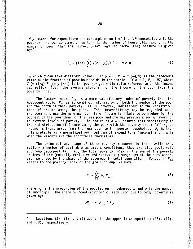
If y; stands for expenditure per consumption unit of the ith household, z is thepoverty line per consumption unit, n is the number of households, and q is thenumber of poor, then the Foster, Greer, and Thorbecke (FGT) measure is givenby:9

The latter index, PI' is a more satisfactory index of poverty than theheadcount ratio, Po, as it combines information on both the number of the poorand the depth of their poverty. It is, however, indifferent to the redistribu­t ion of income among the poor. Th is insens it ivi ty may be regarded as ashortcoming since the marginal utility of income is likely to be higher for thepoorest of the poor than for the less poor and one may presume a social aversionto extreme levels of poverty. The choice of a = 2 ensures this sensitivity tothe redistribution of income among the poor with the poverty index falling asincome is transferred from the less poor to the poorer households. P2 is theninterpretable as a normalized weighted sum of expenditure (income) shortfallswhen the weights are the shortfalls themselves.

The principal advantage of these poverty measures is that, while theysatisfy a number of desirable axiomatic conditions, they are also additivelysubgroup decomposable, i.e., the total poverty index is the sum of the povertyindices of the (mutually exclusive and exhaustive) subgroups of the population,each weighted by the share of the subgroup in total population. Hence, if Pj ••

refers to the poverty index of the jth subgroup, we have:

in which a can take different values. If a = 0, Po = H (=qjn) is the headcountratio or the fraction of poor households in the sample. If a = 1, PI = HI, whereI (= (1jq) L [(Z-Yi)jZ]) is the poverty gap ratio (also referred to as the incomegap rat i0), i. e., the average short fall of the income of the poor from thepoverty line.

(4)

9 Equations (2), (3), and (5) appear in the appendix as equations (15), (17),and (18), respectively.

-21-

It is the property of decomposability that permits us to create a profileof poverty in each of the two areas under consideration. This profile providesa decompos it i on of total poverty by selected criteri a, such as occupat i ona1category of the household head or his or her education, household size, etc.

The FGT index is now routinely employed in the literature on poverty. Asimilar index has recently been proposed by Ray (1989). It is written as:

q

Pa = (g/nz) E (91

/ g)a (5)1 -1

where g = (l/q) L 9; is the "mean poverty gap." It differs from the FGT indexin that the income gap of the poor in the expression on the right-hand side ofthe summation sign is divided by the mean poverty gap rather than by the povertyline as in the FGT index. The Ray index satisfies the same axioms as the FGTindex and some more besides (see the appendix). The poverty profiles of Kinshasaand Bandundu Town in Section 5 report both these indices side by side for acomparison (see Tables 14 and 15).

4. POVERTY AND FOOD CONSUMPTION: A PRELIMINARY ANALYSIS

This section is concerned with the preliminary stages of the analysis ofpoverty in Kinshasa and Bandundu Town. It describes the calculation of householdsize in consumption units, the estimation of calorie "consumption,1I and thechoice of the recommended dietary allowance of calories. The section thenpresents some prel iminary results focusing on differences in major householdcharacteristics by expenditure category.

HOUSEHOLD SIZE IN "CONSUMPTION UNITS"

Households differ in size and composition. These differences have to beaccounted for when compari ng certain types of household data, for exampleexpenditures. A common approach is to use conversion coefficients that expressthe needs of each individual member, normally in terms of calories, relative tothat of a "consumption unit," typically an adult. These coefficients are thenaggregated for each household to determine its size in "consumption units." Thevariables of interest can be normalized by dividing them by this indicator toimprove interhousehold comparisons.

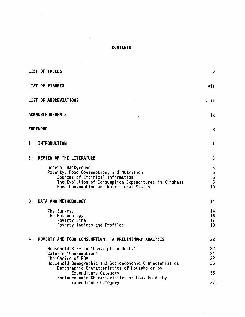
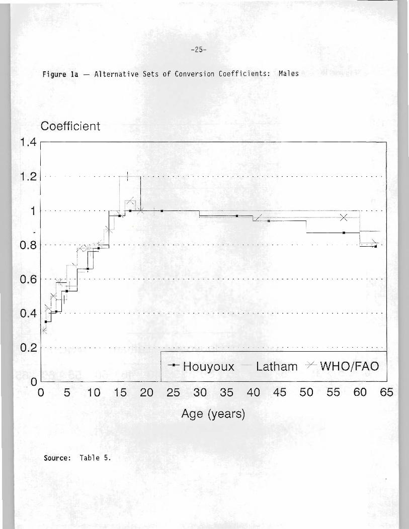
Houyoux (1973) made the first attempt to use such conversion coefficientsin Zaire. He applied them in the analysis of his 1969 Kinshasa survey data.Houyoux derived the age- and sex-specific coefficients while estimating theappropriate level· of the recommended dietary allowance (RDA) of calories inKinshasa (see below). The procedure amounts to simply dividing the RDA of eachtype of individual, as specified by the FAD (1957), by that of the "consumptionunit," a 25-year-old male of 65 kg (the average weight of male adults inKinshasa). This procedure yielded the coefficients for individuals up to 19years of age; for those 20 or more the coefficients were assumed. The resultsare presented in Table 5, top panel.

Because the FAD source from which some of the coefficients are derived datesback to the 1950s and the rest are assumed by Houyoux himself, it would beinstructive to compare this set of coefficients with others that exist. Two ofthese are presented in the middle and bottom panels of Table 5. The former(Latham 1965) is recommended specifically for East Africa, and the latter (WHO1990) is the latest in the series of official recommendations that are issuedfrom time to time by the FAO or WHO. 10 The comparison is best made graphically.

10 WHO (1990) gives FAD (l987) as a source and provides recommended dietaryintakes with respect to energy for various age groups. The coefficients arecalculated by dividing the recommended intake of each group by that of a 25-year­old man weighing 65 kg, our consumption unit, which is 2,700 kcal.

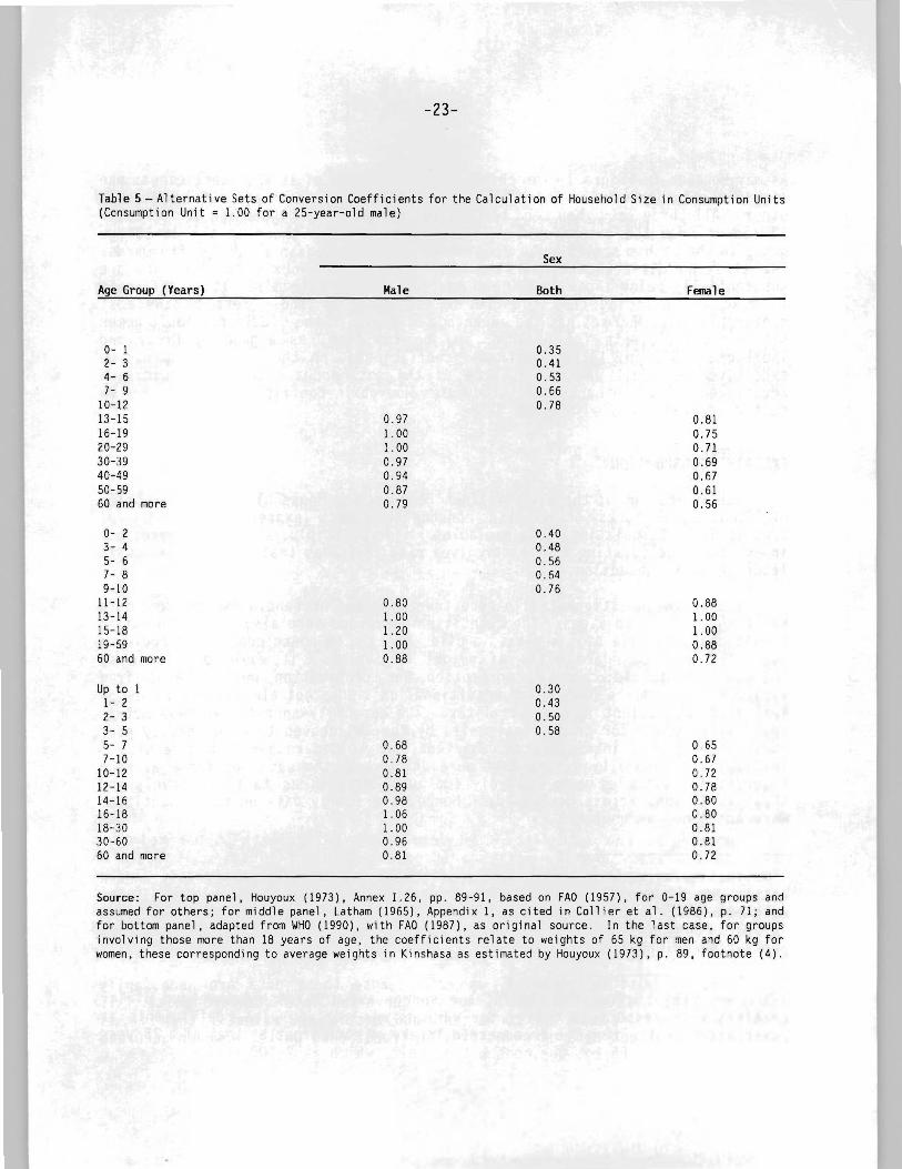
-23-

Table 5 - Alternative Sets of Conversion Coefficients for the Calculation of Household Size in Consumption Units(Consumption Unit = 1.00 for a 25-year-old male)

Sex

Age Group (Years) Hale Both Female

0- 1 0.352- 3 0.414- 6 0.537- 9 0.66

10-12 0.7813-15 0.9716-19 1. 0020-29 1. 0030-39 0.9740-49 0.9450-59 0.8760 and more 0.79

0- 2 0.403- 4 0.485- 6 0.567- 8 0.649-10 0.76

11-12 0.8013-14 1. 0015-18 1. 2019-59 1. 0060 and more 0.88

Up to 0.301- 2 0.432- 3 0.503- 5 0.585- 7 0.687-10 0.78

10-12 0.8112-14 0.8914-16 0.9816-18 1. 0618-30 1. 0030-60 0.9660 and more 0.81

0.810.750.710.690.670.610.56

0.881. 001. 000.880.72

0.650.670.720.780.800.600.610.610.72

Source: For top panel, Houyoux (1973), Annex 1.26, pp. 69-91, based on FAD (1957), for 0-19 age 9rouPS andassumed for others; for middle panel, Latham (1965), Appendix 1, as cited in Collier et a1. (1986), p. 71; andfor bottom panel. adapted from WHD (1990), with FAD (1987), as original source. In the last case, for groupsinvolving those more than 18 years of age, the coefficients relate to weights of 65 kg for men and 60 kg forwomen, these corresponding to average weights in Kinshasa as estimated by Houyoux (1973), p. 89, footnote (4).

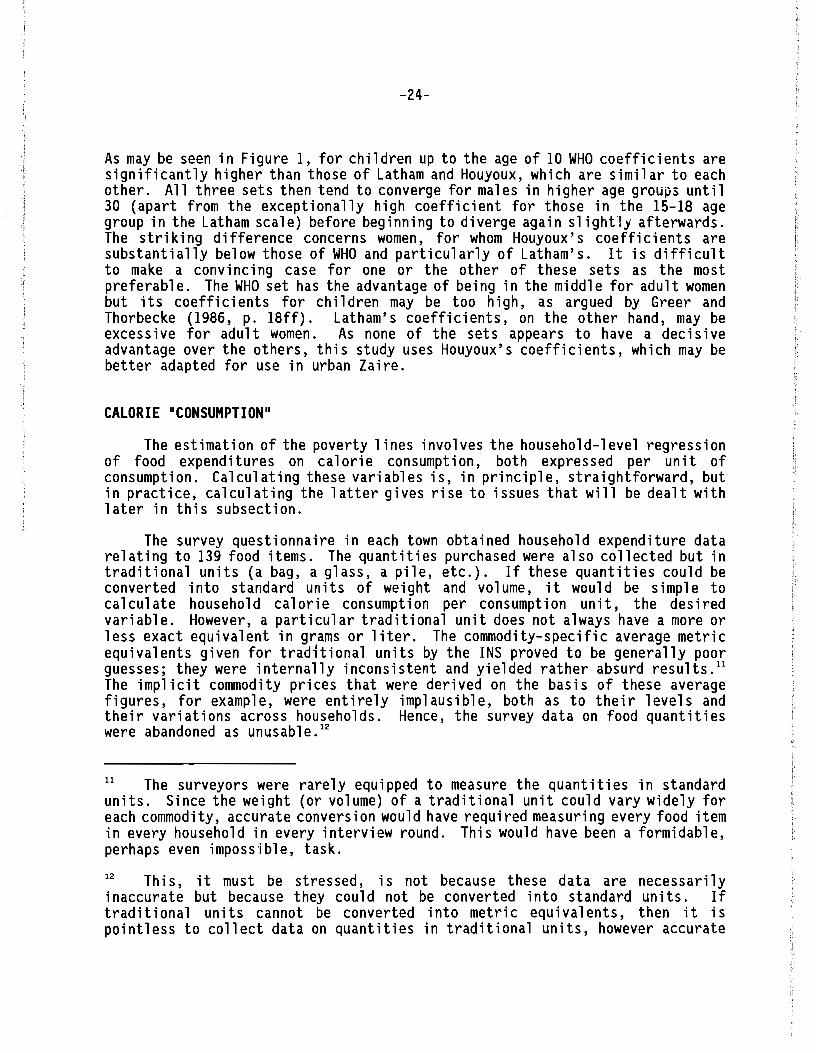
-24-

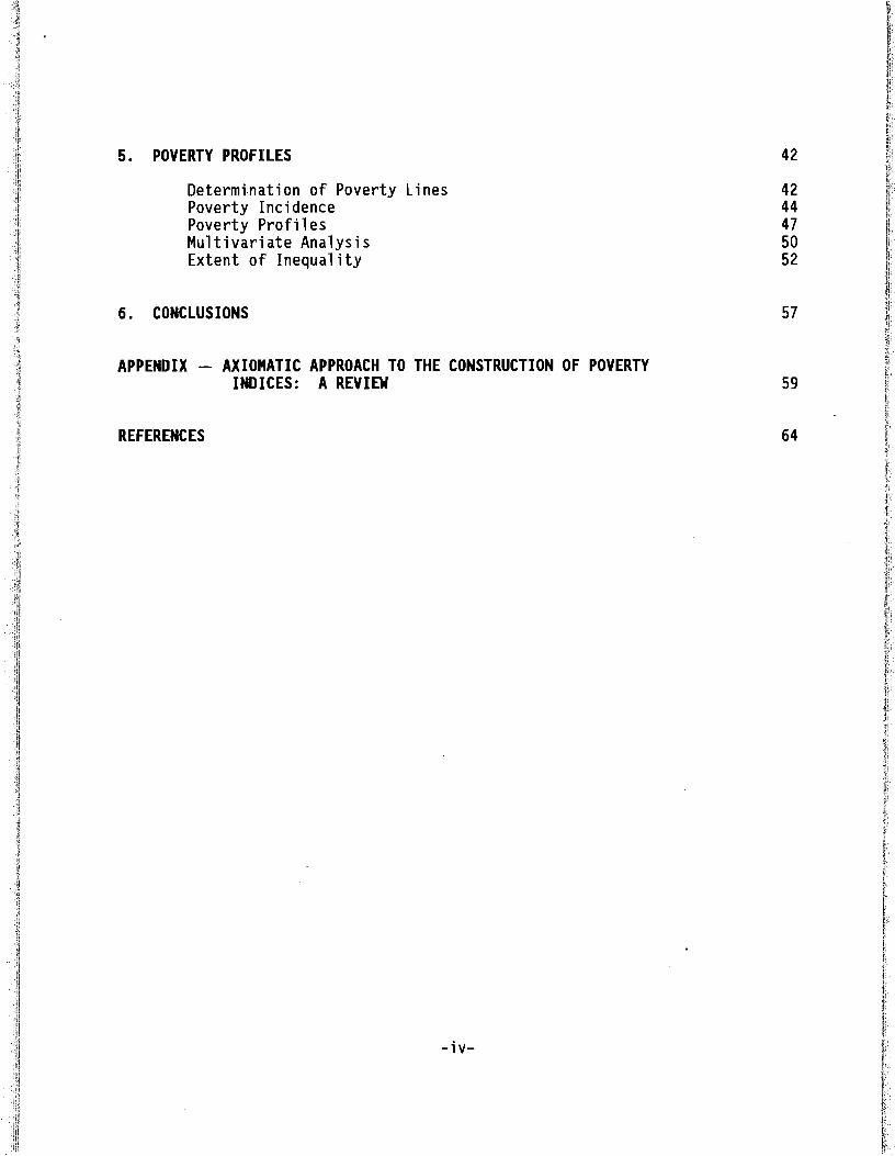
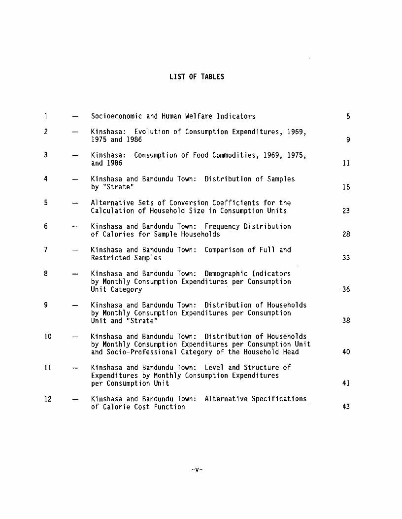
As may be seen in Figure 1, for children up to the age of 10 WHO coefficients aresignificantly higher than those of Latham and Houyoux, which are similar to eachother. All three sets then tend to converge for males in higher age groups until30 (apart from the exceptionally high coefficient for those in the 15-18 agegroup in the Latham scale) before beginning to diverge again sl ight"!j afterwards.The striking difference concerns women, for whom Houyoux's coefficients aresubstantially below those of WHO and particularly of Latham's. It is difficultto make a convincing case for one or the other of these sets as the mostpreferable. The WHO set has the advantage of being in the middle for adult womenbut its coefficients for children may be too high, as argued by Greer andThorbecke (1986, p. 18ff). Latham's coefficients, on the other hand, may beexcessive for adult women. As none of the sets appears to have a decisiveadvantage over the others, this study uses Houyoux's coefficients, which may bebetter adapted for use in urban Zaire.

CALORIE "CONSUMPTION"

The estimation of the poverty lines involves the household-level regressionof food expenditures on calorie consumption, both expressed per unit ofconsumption. Calculating these variables is, in principle, straightforward, butin practice, calculating the latter gives rise to issues that will be dealt withlater in this subsection.

The survey questionnaire in each town obtained household expenditure datarelating to 139 food items. The quantities purchased were also collected but intraditional units (a bag, a glass, a pile, etc.). If these quantities could beconverted into standard units of weight and volume, it would be simple tocalculate household calorie consumption per consumption unit, the desiredvariable. However, a particular traditional unit does not always have a more orless exact equivalent in grams or liter. The commodity-specific average metricequivalents given for traditional units by the INS proved to be generally poorguesses; they were internally inconsistent and yielded rather absurd results. 11

The implicit commodity prices that were derived on the basis of these averagefigures, for example, were entirely implausible, both as to their levels andtheir variations across households. Hence, the survey data on food quantitieswere abandoned as unusabl e. 12

11 The surveyors were rarely equipped to measure the quantities in standardunits. Since the weight (or volume) of a traditional unit could vary widely foreach commodity, accurate conversion would have required measuring every food itemin every household in every interview round. This would have been a formidable,perhaps even impossible, task.

12 This, it must be stressed, is not because these data are necessarilyinaccurate but because they could not be converted into standard units. Iftraditional units cannot be converted into metric equivalents, then it ispointless to collect data on quantities in traditional units, however accurate

-25-

Figure la --- Alternative Sets of Conversion Coefficients: Males

Coefficient1.4r-----------------------------,

,.......:-~---'----------,-_..._-- tz~======~--"7·/;:-----l' . -...---- ._-;-r'- ,

1 ... ---- ..... -

1.2 ... --. -.. -.... ---III .'

7,1,

0.8 "- . . - . . .[~~\c; .-:-'i

I'"••__..1..

'... _ __ ._- .. - - _ .. __ . __ .--.--_.----.~.

o.6 ...~~ ~~~ . -. . .. -. . . . . . . . --. --. . . . . . . . . - . . . . . . . . - .. ---. - . . -. . . --. -. . . . . .

r<"I~"1 .

0.4

0.2

-- Houyoux - Latham -7)/.- WHO/FAaOL..------------.l------------------o 5 10 15 20 25 30 35 40 45 50 55 60 65

Age (years)

Source: Table 5.

-26-

Figure lb -- Alternative Sets of Conversion Coefficients: Females

Coefficient1.2 r-------------------------------,

1 -. -. - - ..,---+-------,- - - .. - , .. -. - - .. - --

0.8

0.6

~/ '/ I..... ,'.; ~.:o .· c.C~··c ~---.. - "'-T_<'.. ,.. .." .~'------ .....---

~:..., " I•------- -.- ---- -- -- -.. ---"'--'---L'

; I

, ~ I0.4 .r· - ----- - - - 'I"

0.2 -

- Houyoux-- Latham y. WHO/FADo IL---- ----'-- ----'

o 5 10 15 20 25 30 35 40 45 50 55 60 65

Age (years)

Source: Table 5.

-27-

Parallel to the main surveys, the INS had also carried out price surveys inthe main food markets of Kinshasa and Bandundu Town. The surveyors hadsystematically measured the quantities in standard units on site. The averageprice per kilogram or liter of each item in each town are reported in INS (1989cand 1989d). We have relied on these average prices to estimate the purchasedquantities of various food items for each sample household. These quantitieswere then converted into calories,lJ summed over all food items, and divided byhousehold size in consumption units to estimate the household calorie purchaseper consumption unit.

The use of a citywide average price to arrive at the purchased quantity ofeach food is a common practice that would not bias the results unduly if allsample households paid more or less the same price. Where this is not the case,a bias is introduced in the derived quantity figures. Poorer households tend topay less than average prices and richer ones more. For a given food expenditure,therefore, the use of a single average price for all households would understatethe quantity (calories) purchased by the poor and to overstate that by the rich.The derived calorie distribution is, therefore, flatter and displays greatervariation than the actual distribution. Thus, while exceedingly low orexceedingly high calorie figures are 1ikely to suggest erroneous food expendituredata, a certain amount of underestimation at the lower end of the distributionand some overestimation at the higher end is to be expected and would not signifyinaccuracy in the underlying data. This fact must be borne in mind in selectingan "acceptable" range for the calorie variable (see below).

Another source of bias is the difference between consumption and expendi­ture: a11 foods purchased duri ng the surveys' reference peri ods are notnecessarily consumed during that same period. This difference is less likely tobe consequential in Kinshasa, where the survey period was a full year, than inBandundu Town, where it was only one month. The quest ion of seasonality,therefore, may arise in the latter case although not much can be done about it.

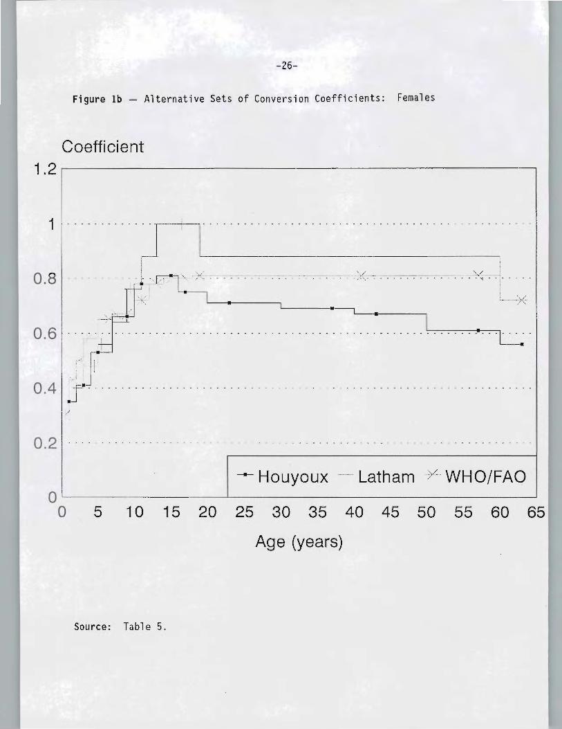
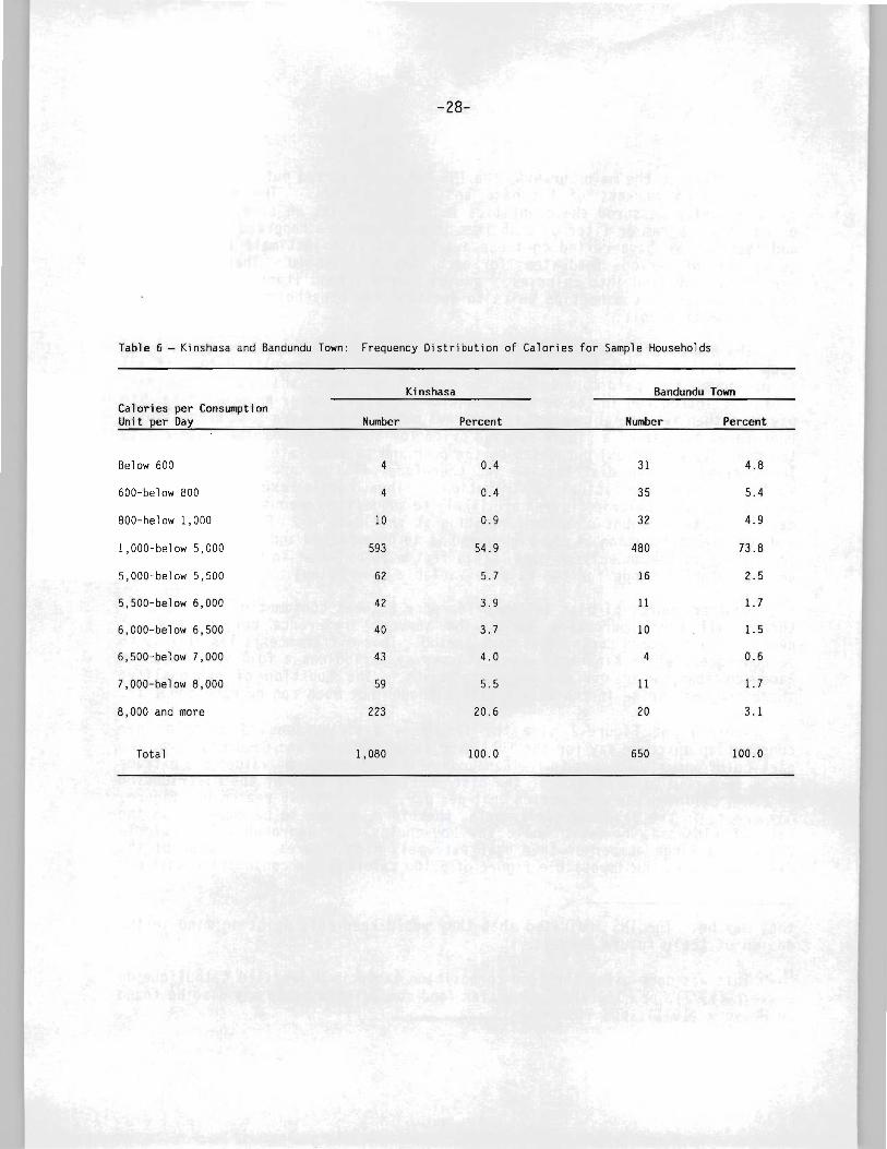
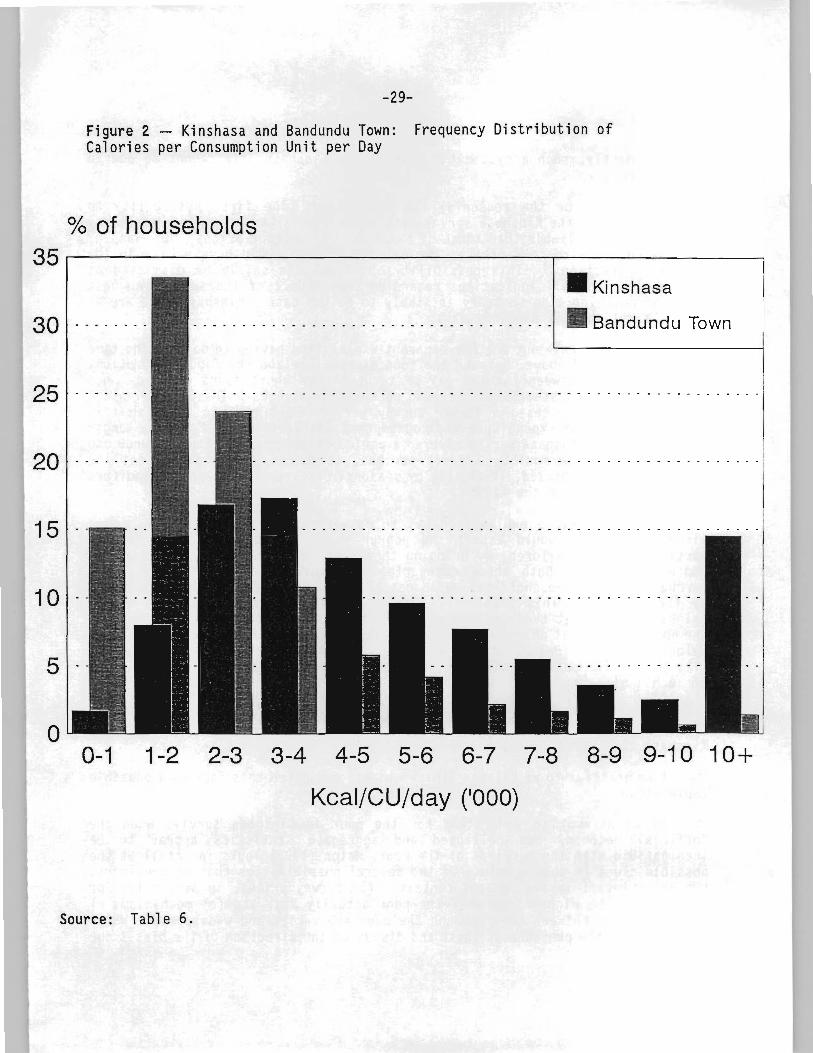
Table 6 and Figure 2 give the frequency distributions of calories perconsumption unit per day for the full samples of Kinshasa and Bandundu Town. Noparticular anomaly appears in the Bandundu distribution: some values are extremeto be sure, but at both ends of the distribution. The mean of the distributionis 2,744 calories per consumption unit per day, an apparently reasonable figure.Any errors in the Bandundu survey data, therefore, appear to be random. In thecase of Kinshasa, however, while few households have improbably low caloriefigures, a large number of them have extremely high figures. The mean of thedistribution is the impossible figure of 6,106 calories per consumption unit per

they may be. The INS indicated that they would keep this point in mind in thedesign of their future surveys.

13 This was done using the food composition table in Universite Catholique deLouvain (1977), pp. 167-172. Asimilar food composition table may also be foundin Houyoux (1971), pp. 118-142.

-28-

Table 6 - Kinshasa and Bandundu Town: Frequency Distribution of Calories for Sample Households

Kinshasa Bandundu TownCalories per ConsumptionUnit per Day Number Percent Number Percent

Below 600 4 0.4 31 4.8

600-below 800 4 0.4 35 5.4

800-below 1,000 10 0.9 32 4.9

l,OOO-below 5,000 593 54.9 480 73.8

5,OOO-below 5,500 62 5.7 16 2.5

5,500-below 6,000 42 3.9 11 1.7

6,000-below 6,500 40 3.7 10 1.5

6,500-below 7,000 43 4.0 4 0.6

7,000-below 8,000 59 5.5 11 1.7

8,000 and more 223 20.6 20 3.1

Total 1,080 100.0 650 100.0

-29-

Figure 2 -- Kinshasa and Bandundu Town: Frequency Distribution ofCalories per Consumption Unit per Day

% of households35 r------------------,.----------,

30 ... -.. -.

25 -.

20 '" -.-_.

15 ..

10 ..

5 ..

o

• Kinshasa

Bandundu Town

I. . - .. - . '. - - . - ..... - - .. - .... - .. - .. - .. - - . - - . - - . - - . - - - - _!

0-1 1-2 2-3 3-4 4-5 5-6 6-7 7-8 8-9 9-10 10+

Kcal/CU/day ('000)

Source: Table 6.

-30-

dayl Evidently, such a systematic bias in the Kinshasa data cannot be due torandom errors.

What might be the reason(s) for this bias? The first possibility toconsider is that the Kinshasa survey data (food expenditures and/or prices) maysimply be less reliable than those of Bandundu. If average prices, for example,are biased downward in Kinshasa, the calorie figures would have a bias in theopposite direction. 14 This possibility, however, can safely be dismissed asimprobable since all indications regarding the conduct of the surveys s~ggest

that, if anything, the contrary is likely to be the case. Kinshasa data are atleast as reliable as Bandundu data.

We can also rule out another apparent explanation having to do with the timelag, as mentioned above, between the food expenditure and the food consumption.While the link between the two may be tenuous over short spans of time (whenexpenditures can systematically exceed consumption as households take advantageof low seasonal prices), a longer survey period would tend to diminish thisdiscrepancy. Food expenditure and consumption would average out over a longertime span. The Kinshasa survey covered a period of one year but the Bandundu oneconcerned only one month. Ceteris paribus, therefore, one would expect theformer to be less biased, if at all, by seasonal discrepancy between expenditureand consumption than the latter.

A more plausible explanation has to do with cultural obligations: manyricher households would assist the poorer members of the extended family,particularly the children, by bringing them over to live with them. They alsoemploy servants. Both these categori es share in the consumption of foodspurchased by the household but would not have counted as its bona fide membersby the survey.lS This possibility, which would give an upward bias to thecalorie variable at the high end of the income scale, accords rather well withthe observation that only the Kinshasa sample suffers significantly from inflatedcalorie figures. (Both practices are likely to be far more common in the capitalcity than in the poorer Bandundu.) We have no indication, however, of the extentof such a bias. 16

14 Average prices for the major food items were almost always higher inKinshasa than in Bandundu, often substantially.

15 I am grateful to wa Bilenga Tshishimbi who suggested this fact as a possibleexplanation.

16 In an attempt to understand how the poor in Kinshasa survive when the"official" economy has collapsed and aggregate statistics appear to beincompatible with the survival of the poor, Maton (1992) looks in detail at thepossible clues to this puzzle. Of the several possibilities that he considers,two are relevant in the present context: (a) survey prices, in particular forcassava, may be higher than what the poor actually pay; and (b) mechanisms ofredistribution between the rich and the poor are varied and widespread. Whilewe have noted the presence of these and discussed the direction of the biases due

-31-

Survey data of the kind under consideration often yield values of caloriesper consumption unit per day, which are outside of a "reasonable" range. In asimilar study of rural Kenya, for example, some 23 percent of the observationshad to be excluded because the resulting values of this variable were outside ofa 1,000-5,000 range, or the implied consumption of some major food items wereexcessive (Greer and Thorbecke 1986, Appendix A). Another study on Ghana imposeda range of 800-5,500 as realistic from a nutritional viewpoint but did notspecify the proportion of the observations that were thereby excluded (Kyeremeand Thorbecke 1987, p. 1198).

In our case, the choice of any "reasonable" range would el iminate anoverwhelming proportion of higher-income sample households in Kinshasa. InBandundu Town households at both ends of the scale would be eliminated more orless equally. In the less problematic case of Bandundu, where there is nothingunusual about the frequency distribution, a range of 800-6,000 calories perconsumption unit per day has been selected to identify usable observations. Thisrange was chosen after a series of experimental runs and consultations withZairian experts. It is slightly larger than is normally allowed on nutritionalgrounds alone (see above) because two additional factors, working in oppositedirections, were also considered in setting the limits. On the one hand, asmentioned earlier, our use of average commodity prices leads to calorie figureswhose distribution is more spread out than is actually the case. A wider rangeretains some of the observations with accurate data that would otherwise havebeen unjustifiably excluded because of the inherent bias in the method ofcalculating the calorie variable. On the other hand, the range cannot be allowedto be too wide because of the risk of including observations for which foodpurchases do indeed differ from consumption during the survey period (apotentially serious problem in Bandundu where the survey period was only onemonth). The selected range is therefore a compromise, intended to strike abalance between the need to retain accurate observations and the necessity ofexcluding erroneous observations or observations with significant divergencebetween expenditure and consumption. The choice of the 800-6,000 range retained539 observations out of a total sample size of 650 in Bandundu Town (a "loss" of17 percent of the sample).

Similar considerations also influenced the selection of the range inKinshasa, but the upper limit is set at the higher level of 7,000 on account ofthe greater diversity of prices,17 hospitality given to poorer members of the

to them, these factors are probably insufficient to account for the excessivelevel of average calorie figure in Kinshasa and particularly for its distributionin the sample.

17 Prices in Kinshasa for the same item are likely to vary much more than inBandundu Town because, among other reasons, of the greater diversity in the typeand quality of foods available (Kinshasa being many times larger than BandunduTown). Tollens et al. (1992), for example, found a wide divergence in the pricesof a key staple food, cassava, in the different markets of Kinshasa (cited inMaton 1992, p. 2).

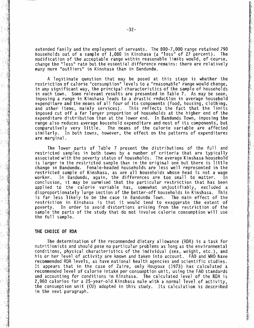
-32-

extended family and the employment of servants. The 800-7,000 range retained 790households out of a sample of 1,080 in Kinshasa (a "loss" of 27 percent). Themodification of the acceptable range within reasonable limits would, of course,change the "loss" rate but the essential difference remains: there are relativelymany more "outliers" in Kinshasa than in Bandundu.

A legitimate question that may be posed at this stage is whether therestriction of calorie "consumption" levels to a "reasonable" range would change,in any significant way, the principal characteristics of the sample of householdsin each town. Some relevant results are presented in Table 7. As may be seen,imposing a range in Kinshasa leads to a drastic reduction in average householdexpenditure and the means of all four of its components (food, housing, clothing,and other items, mainly services). This reflects the fact that the limitsimposed cut off a far larger proportion of households at the higher end of theexpenditure distribution than at the lower end. In Bandundu Town, imposing therange also reduces average household expenditure and most of its components, butcomparatively very little. The means of the calorie variable are affectedsimilarly. In both towns, however, the effect on the patterns of expendituresare marginal.

The lower parts of Table 7 present the distributions of the full andrestricted samples in both towns by a number of criteria that are typicallyassociated with the poverty status of households. The average Kinshasa householdis larger in the restricted sample than in the original one but there is littlechange in Bandundu. Female-headed households are less well represented in therestricted sample of Kinshasa, as are all households whose head is not a wageworker. In Bandundu, again, the differences are too small to matter. Inconclusion, it may be surmised that the particular restriction that has beenapplied to the calorie variable has, somewhat unjustifiably, excluded adisproportionately large section of the better-off households in Kinshasa. Thisis far less likely to be the case in Bandundu Town. The main effect of therestriction in Kinshasa is that it would tend to exaggerate the extent ofpoverty. In order to avoid distortions arising from the restriction of thesample the parts of the study that do not involve calorie consumption will usethe full sample.

THE CHOICE OF RDA

The determination of the recommended dietary allowance (RDA) is a task fornutritionists and should pose no particular problems as long as the environmentalconditions, physical characteristics of the individual (sex, weight, etc.), andhis or her level of activity are known and taken into account. FAD and WHD haverecommended RDA levels, as have national health agencies and scientific studies.It appears that in the case of Zaire, only Houyoux (1973) has calculated arecommended level of calorie intake per consumption unit, using the FAD standardsand accounting for conditions in Kinshasa. The calculated level of the RDA is2,960 calories for a 25-year-old Kinshasa male with a normal level of activity,the consumption unit (CU) adopted in this study. Its calculation is describedin the next paragraph.

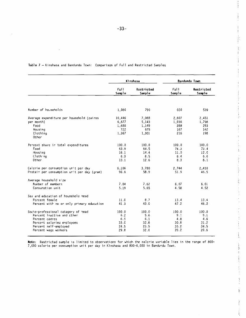
-33-

Table 7 - Kinshasa and Bandundu Town: Comparison of Full and Restricted Samples

Kinshasa Bandundu Town

Number of households

Average expenditure per household (zairesper month)

FoodHousingClothingOther

Percent share in total expendituresFoodHousingClothingOther

Calorie per consumption unit per dayProtein per consumption unit per day (gram)

Average household sizeNumber of membersConsumption unit

Sex and education of household headPercent femalePercent with no or only primary education

Socio-professional category of headPercent inactive and otherPercent cadresPercent salaried employeesPercent self-employedPercent wage workers

FullSample

1,080

10,4466,6771,680

7221,367

100.063.916.16.9

13.1

6,10696.6

7.045.19

11. 041.3

100.06.26.5

33.024.529.8

RestrictedSample

790

7,9685,1431,149

6751,001

100.064.514.48.5

12.6

3,78058.9

7.625.65

8.743.0

100.05.66.1

32.823.532.0

FullSample

650

2,6071,936

288167216

100.074.311.06.48.3

2,74451.9

6.074.58

13.447.2

100.09.14.8

30.835.220.2

RestrictedSample

539

2,4511,798

293162198

100.073.412.06.68.1

2,41046.5

6.014.52

13.446.2

100.09.14.6

31.234.520.6

Note: Restricted sample is limited to observations for which the calorie variable lies in the range of 800­7,000 calorie per consumption unit per day in Kinshasa and 800-6,000 in Bandundu Town.

The comparisons are approximate because the age ranges are not the same.

-34-

Assuming that the population is divided equally between males and females,the simple average of Houyoux's figures, 2,960 for a male adult and 2,099 for afemale one, yields an RDA of 2,530 for an adult. This average may be comparedwith the basic RDA of 2,250 in the Kenya study (which is 9 percent lower) and thecalculated average figure of 1,880 in the Ghana study (26 percent lower).18Accordingly, we shall treat the Houyoux RDA as the "high" variant in ouranalysis.

The point of departure for Houyoux's procedure (1973, Annex 1.26, pp. 89-92)is to adopt the FAO-specified level of 3,200 kcals per day for a 25-year-old maleof 65 kg 1i vi ng in an area with a mean temperature of 10°C and engaged in"normal" activities. The average weight of male adults in Kinshasa, heestimated, was 65 kg but the mean temperature was 25°C. The adjustment fortemperature difference was made by reducing calorie requirements by 0.5 percentfor each 1°C rise in temperature (a total of 7.5 percent in this case). A 25­year-old male in Kinshasa is therefore estimated to require 2,960 kcals per day.A similar procedure for a 25-year-old female weighing 59 kg yielded, startingfrom the FAO figure of 2,269 kcals per day, an RDA of 2,099 kcals in Kinshasa (71percent of the corresponding figure for a male counterpart).

Is the level of RDA for a consumption unit as calculated above, 2,960 kcalsper day, an appropriate level for use in this study? Without entering into thevariety of arguments that oppose nutritionists in setting the m"inimum levelrequired, it may be noted that various poverty studies have used rather differentRDAs. Thi s fact underl i nes the somewhat arbi trary nature of the resul t i ngpoverty est imates since the 1eve1 of the RDA is a major determi nant of thepoverty incidence. FAO-recommended 1evel s, it has sometimes been argued,exaggerate average requirements, ignoring intra-individual (over time) and inter­individual differences. Greer and Thorbecke (1986) appear to share this view anduse a basic RDA of 2,250 kcals per adult equivalent (defined as any male orfemale above 15 years of age) in their analysis of Kenyan smallholders. Giventhe uncertainty, they also carry out a sensitivity test of the results using twoother RDA levels, one 15 percent below the basic level and another 15 percentabove. In the Ghana study mentioned earl ier, Kyereme and Thorbecke (1987,pp. 1190-1191, and Note 5, p. 1198) used the FAO-recommended level of 2,092 kcalsper adult equivalent, based on adult weights of 58 kg (male) and 50 kg (female),with sensitivity tests involving figures that are 10 percent below and above thebasic level. It appears, however, that in this study an adult equivalent isactually a ma7e person of 15 years of age and above since the coefficient appliedto a female adult is 0.8 (Kyereme and Thorbecke 1986). If this interpretationis correct, the basic RDA for an adult equivalent would be only 1,880 when anadult is equally likely to be male or female. Finally, the WHO source referredto earlier recommends, following another FAO recommendation (FAO 1987), a levelof 2,700 for a man and one of 2,200 for a woman in the 18-30 age bracket (WHO1990, p. 168).

18

-35-

Ben-Senia (1991), in his analysis of rural Bandundu, also regards the FAO­norms-based Houyoux estimate of 2,960 for a (male) consumption unit (which headjusts slightly upward to 3,000 to account for the more strenuous work performedby the rural populations) as too high. His sensitivity tests use several lowerfigures as well, of which the lowest, 2,550, is his preferred alternative. Thisis 15 percent lower than the starting figure and is considered more realistic,in part because the measured calorie intakes in his survey were "certainlyunderestimated" (Ben-Senia 1991, pp. 26-27). Partly to be able to compare urbanand rural areas in Bandundu, we also adopt a variant with an RDA that is 15percent lower than the high case, i.e., 2,516.

As the final variant in our sensitivity tests, we opt for an RDA level thatis 30 percent lower than the "high" case. This implies a figure of 2,072 for a(male) consumption unit, which is just below the basic level used in the Ghanastudy, i.e. 2,092 for a (male) adult equivalent. We consider this level to bemuch too low to provide realistic estimates of the extent of poverty in ouranalysis. This level is probably more appropriate for identifying "extreme"poverty, but the justification for its adoption is simply to have a wide enoughrange for the RDA in tests of sensitivity. Our "high," "medium," and "low"variants for the RDA are, therefore, 2,960, 2,516, and 2,072 calories per day,respectively, for a (male) consumption unit. The middle figure probably comesclosest to what an "appropriate" RDA level would have been for our study, had itbeen known.

HOUSEHOLD DEMOGRAPHIC AND SOCIOECONOMIC CHARACTERISTICS

In a preliminary effort to identify the differences in characteristicsbetween poorer and richer households (i .e., before poverty lines are establishedin the next section), sample households are grouped by the level of monthlyconsumption expenditures (MCE) per consumption unit (CU). These compriseexpenditures on food, lodging, clothing, and other items that are intended forthe actual consumption of household members. They exclude expenditures on itemsto be given away (gifts, etc.), to be resold, or to be used in household businessactivities (which collectively constitute nonconsumption expenditures).

Four categories of households are identified in each of the two urbancenters (Kinshasa and Bandundu Town) by the level of MCE per CU: the poorest 30percent of households (LOW30), the next 30 percent with intermediate levels ofthe variable (MED30), the richer 30 percent (HIGH30), and the richest 10 percentof households (TOPI0). This grouping of households is designed to be both simpleand able to capture the essential differences that may exist between poorer andricher households.

Demographic Characteristics of Households by Expenditure Category

Table 8 assembles the results relating to some household demographiccharacteristics by expenditure category. Kinshasa households are fairly large,averaging seven members. The average household in Bandundu Town is somewhat

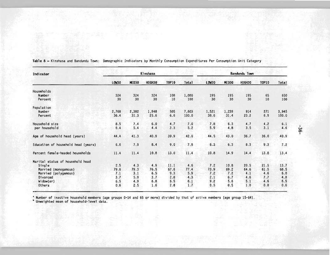
Table 8 - Kinshasa and Bandundu Town: Demographic Indicators by Monthly Consumption Expenditures Per Consumption Unit Category

Indicator Kinshasa Bandundu Town

l0W30 MED30 HIGH30 TOP10 Total l0W30 MED30 HIGH30 TOPIO Total

HouseholdsNumber 324 324 324 108 1,080 195 195 195 65 650Percent 30 30 30 10 100 30 30 30 10 100

PopulationNumber 2,768 2,382 1,948 505 7,603 1,521 1,239 914 271 3,945Percent 36.4 31.3 25.6 6.6 100.0 38.6 31.4 23.2 6.9 100.0

Household size 8.5 7.4 6.0 4.7 7.0 7.8 6.3 4.7 4.2 6.1per household 6.4 5.4 4.4 3.3 5.2 5.9 4.8 3.5 3.1 4.6 I

wClI

Age of household head (years) 44.4 41.3 40.9 39.9 42.0 44.5 43.0 36.7 36.0 40.9

Education of household head (years) 6.6 7.9 8.4 9.0 7.8 6.3 6.3 8.3 9.3 7.2

Percent female-headed households 11.4 11.4 10.8 13.0 11. 4 10.8 14.9 14.4 13.8 13.4

Marital status of household headSi ngl e 2.5 4.3 4.9 11. 1 4.6 7.2 10.8 20.5 21.5 13.7Married (monogamous) 79.6 79.3 76.5 67.6 77 .4 73.9 69.2 64.6 61. 5 68.5Married (polygamous) 7.1 3.1 6.5 9.3 5.9 7.2 7.2 4.1 4.6 6.0Divorced 3.7 5.9 3.7 2.8 4.3 2.1 6.7 4.6 7.7 4.8Widow(er) 6.5 4.9 6.8 6.5 6.1 9.2 5.6 5.1 4.6 6.5Others 0.6 2.5 1.6 2.8 1.7 0.5 0.5 1.0 0.0 0.6

• Number of inactive household members (age groups 0-14 and 65 or more) divided by that of active members (age group 15-64).• Unweighted mean of household-level data.

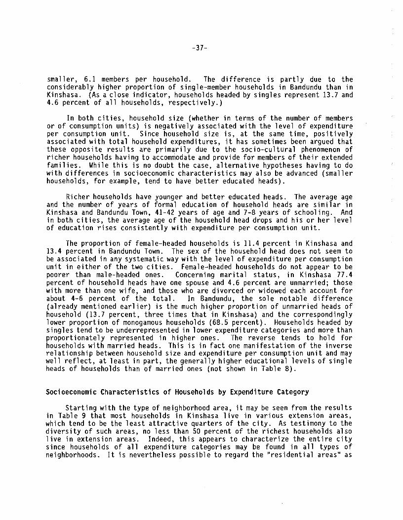
-37-

smaller, 6.1 members per household. The difference is partly due to theconsiderably higher proportion of single-member households in Bandundu than inKinshasa. (As a close indicator, households headed by singles represent 13.7 and4.6 percent of all households, respectively.)

In both cities, household size (whether in terms of the number of membersor of consumption units) is negatively associated with the level of expenditureper consumption unit. Since household size is, at the same time, positivelyassociated with total household expenditures, it has sometimes been argued thatthese opposite results are primarily due to the socio-cultural phenomenon ofricher households having to accom~odate and provide for members of their extendedfamilies. While this is no doubt the case, alternative hypotheses having to dowith differences in socioeconomic characteristics may also be advanced (smallerhouseholds, for example, tend to have better educated heads).

Richer households have younger and better educated heads. The average ageand the number of years of formal education of household heads are similar inKinshasa and Bandundu Town, 41-42 years of age and 7-8 years of schooling. Andin both cities, the average age of the household head drops and his or her levelof education rises consistently with expenditure per consumption unit.

The proportion of female-headed households is 11.4 percent in Kinshasa and13.4 percent in Bandundu Town. The sex of the household head does not seem tobe associated in any systematic way with the level of expenditure per consumptionunit in either of the two cities. Female-headed households do not appear to bepoorer than male-headed ones. Concern ing mari ta1 status, inKi nshasa 77.4percent of household heads have one spouse and 4.6 percent are unmarried; thosewith more than one wife, and those who are divorced or widowed each account forabout 4-6 percent of the total. In Bandundu, the sole notable difference(already mentioned earlier) is the much higher proportion of unmarried heads ofhousehold (13.7 percent, three times that in Kinshasa) and the correspondinglylower proportion of monogamous households (68.5 percent). Households headed bysingles tend to be underrepresented in lower expenditure categories and more thanproportionately represented in higher ones. The reverse tends to hold forhouseholds with married heads. This is in fact one manifestation of the inverserelationship between household size and expenditure per consumption unit and maywell reflect, at least in part, the generally higher educational levels of singleheads of households than of married ones (not shown in Table 8).

Socioeconomic Characteristics of Households by Expenditure Category

Starting with the type of neighborhood area, it may be seen from the resultsin Table 9 that most households in Kinshasa live in various extension areas,which tend to be the least attractive quarters of the city. As testimony to thediversity of such areas, no less than 50 percent of the richest households alsolive in extension areas. Indeed, this appears to characterize the entire citysince households of all expenditure categories may be found in all types ofneighborhoods. It is nevertheless possible to regard the "residential areas" as

-38-

Table 9 - Kinshasa and Bandundu Town: Distribution of Households by Monthly Consumption Expenditures perConsumption Unit and Strate

Percent of Households "CEfelT'

Strate LOW30 HED30 HIGH30 TOPI0 Total Heanb (za ires)

KinshasaQuartiers residentiels 2.5 3.4 4.3 13.9 4.4 9,862Anciennes cites 3.4 5.9 6.8 6.5 5.5 3,837Nouve11 es ci tes 14.2 11. 7 12.0 9.3 12.3 2,318Cites planifiees 13.0 9.6 11.4 20.4 12.2 2,592Quartiers d'extension 67.0 69.4 65.4 50.0 65.6 2,060

Total 100.0 100.0 100.0 100.0 100.0 2,385

Bandundu TownQuartiers residentiels 1.0 2.6 1.5 10.8 2.6 2,006Nouve11 es cites 74.4 72 .8 68.7 63.1 71.1 662Quartiers d'extension 24.6 24.6 29.7 26.2 26.3 715

Total 100.0 100.0 100.0 100.0 100.0 711

• Monthly consumption expenditures per consumption unit.b Unweighted.

-39-

the most privileged, followed by old neighborhoods and planned developments. Newdevelopments come next, followed by the extension areas.

Bandundu Town is much younger than Kinshasa. Some 71 percent of householdslive in new developments which, however, may not be any more attractive thanextension areas where more than a quarter of the town's population lives.Indeed, the mean expenditure per consumption unit is lower in new developmentsthan in extension areas. As with Kinshasa, "residential areas" have a higherconcentration of the rich than the town as a whole, although nearly 90 percentof the rich live elsewhere.

As regards the possible association between the expenditure level and thesocio-professional category of the household head, it may be observed in Table 10that the relationship appears to be particularly weak in Kinshasa. In Bandunduit can more readily be seen that the "cadres" are most heavily represented in thehighest expenditure group and the working class in the lowest. Interestingly,the inactive (sans objet) tend to be rather better off than expected in BandunduTown but not in Kinshasa.

Finally, Table 11 reports some results regarding the level and the structureof expenditures in the four groups in each city. The average expenditure perconsumption unit of the top 10 percent of the sample households is more than 10times that of the lowest 30 percent in both Kinshasa and Bandundu Town. Thestructure of expenditures in each city moves in line with expectations, with theshare of food declining as the average expenditure rises. The poorer status ofBandundu Town relative to Kinshasa may also be seen in the higher share of foodin the average budget. The poorest 30 percent of the Bandundu households spendmore than four-fifths of their expenditure on food.

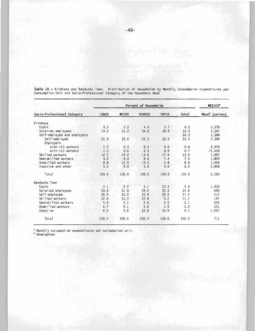
-40-

Table 10 - Kinshasa and Bandundu Town: Distribution of Households by Monthly Consumption Expenditures perConsumption Unit and Socio-Professional Category of the Household Head

Percent of Households HCE/Cu"

Socio-Professional Category LOW30 HE030 HIGH30 TOP10 Total Hean" (zaires)

KinshasaCadre 5.3 2.2 4.0 3.7 6.5 3,578Salaried employees 14.2 31.2 34.6 38.9 33.0 2,347Self-employed and employers 24.5 3,388

Self-employed 21.9 25.0 22.5 23.2 23.2 2,389Employers

with <10 workers 1.5 0.3 0.3 0.0 0.6 6,974with >10 workers 1.2 0.6 0.3 0.9 0.7 31,450

Skilled workers 12.7 14.2 13.6 17.6 13.9 1,997Semiskilled workers 5.2 8.0 8.6 7.4 7.3 1,895Unskilled workers 6.8 10.5 10.5 2.8 8.6 1,954Inactive and other 5.3 8.0 5.6 5.6 6.2 2,896

Total 100.0 100.0 100.0 100.0 100.0 2,385

Bandundu TownCadre 2.1 6.2 3.1 13.9 4.8 1,453Salaried employees 30.8 31.8 29.2 32.3 30.8 685Self-employed 36.9 34.9 35.9 29.2 35.2 617Skilled workers 12.8 13.3 10.8 6.2 11. 7 587Semiskilled workers 4.6 3.1 2.6 0.0 3.1 643Unskilled workers 6.7 5.1 5.6 1.5 5.4 531Inactive 6.2 5.6 12.8 16.9 9.1 1,062

Total 100.0 100.0 100.0 100.0 100.0 711

• Monthly consumption expenditures per consumption unit.b Unweighted.

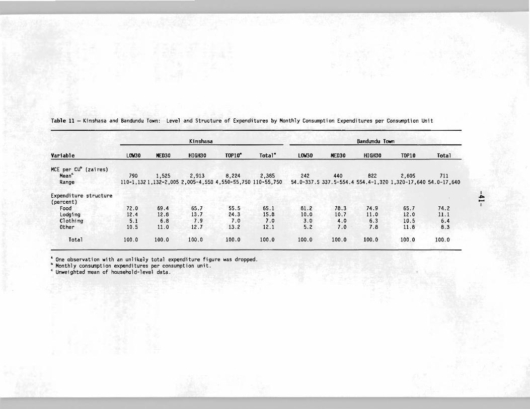
Table 11 - Kinshasa and Bandundu Town: Level and Structure of Expenditures by Monthly Consumption Expenditures per Consumption Unit

Variable L0W30 MED30

Kinshasa

HI6H30 TOPIO" Total- L0W30 MED30

Bandundu Town

HI6H30 TOPI0 Total

MCE per cLf (zaires)Meane

Range790 1,525 2,913 8,224 2,385

110-1,1321,132-2,005 2,005-4,550 4,550-55,750 110-55,750242 440 822 2,605 711

54.0-337.5337.5-554.4554.4-1,320 1,320-17,640 54.0-17,640

Expenditure structure(percent)

FoodLodgingClothingOther

Total

I~......

65.7 55.5 78.3 74.9I

72.0 69.4 65.1 81.2 65.7 74.212.4 12.8 13.7 24.3 15.8 10.0 10.7 11.0 12.0 11.15.1 6.8 7.9 7.0 7.0 3.0 4.0 6.3 10.5 6.4

10.5 11. 0 12.7 13.2 12.1 5.2 7.0 7.8 11.8 8.3

100.0 100.0 100.0 100.0 100.0 100.0 100.0 100.0 100.0 100.0

• One observation with an unlikely total expenditure figure was dropped.b Monthly consumption expenditures per consumption unit.e Unweighted mean of household-level data.

5. POVERTY PROFILES

This section builds on the preparatory work of the preceding one toconstruct poverty profiles for Kinshasa and Bandundu Town in the mid-1980s. Itbegins by describing the determination of poverty lines under differentassumptions and then presents estimates of poverty incidence for various groupsof households in each town. Next, poverty profiles are generated for Kinshasaand Bandundu Town by decomposing total poverty according to household character­istics that were earlier found to be associated with poverty. The main resultsof a multivariate analysis are discussed, and some statistics of inequality arepresented at the end.

DETERMINATION OF POVERTY LINES

The cost-of-calorie function is the basic relationship required to derivethe poverty lines. Alternative functional forms will have different propertiesfrom a theoretical point of view and may differ in the goodness-of-fit to thedata. Several specifications with reasonable properties were tried, and Table 12presents the results of two that are statistically the most significant. Thesemilog specification, used in both the Kenya and Ghana studies mentionedearl i er, assumes that cost per cal ori e ri ses wi th increased consumption ofcalories, and at an ever-increasing rate. 19 This is a reasonable expectationunder many circumstances but the scattergram of our data indicated that thisspecification was not the most appropriate in this instance. The log-logspecification, which assumes a constant elasticity of calorie consumption withrespect to food expenditures, proved to be somewhat better for both cities, asevidenced by the higher values of the coefficient of determination. This resultsuggests that the differences in food composition between the richer and poorerhousehol ds are not dramat i c, at 1east insofar as cost per cal ori e is thecriterion for the differentiation of food items. For th~ base run of the resultsthe selected regression has been used to derive the level of food expenditure perconsumption unit that is necessary to permit meeting the RDA.

In order to estimate the poverty 1ine, food expenditures have to besuppl emented with the mi nimum expendi tures necessary to sat i sfy essent i al nonfoodneeds. The procedures commonly used to arrive at the latter are usually simple

19 This assumption is not necessarily at odds with our earlier use of averageprices for individual food items in the derivation of calorie consumption. Sincefood compos i t ion differs across households, with ri cher ones consumi ng moreexpensive foods than poorer ones, cost per calorie would be higher for the formerwhen all foods are lumped together although it would be the same for all typesof households as far as each particular food item is concerned.

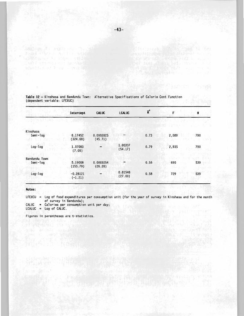
Figures in parentheses are t-statistics.

-43-

Log of food expenditures per consumption unit (for the year of survey in Kinshasa and for the monthof survey in Bandundu);Calories per consumption unit per day;Log of CALUC.

N

539

539

790

790

F

729

690

2,089

2,935

0.56

0.58

0.79

0.73

LCAlUCCAlUCInterCept

Notes:

KinshasaSemi-log 8.17452 0.0002825

(324.68) (45.71)

Log-log 1.07083 1.00307

(7.09) (54.17)

Bandundu TownSemi-log 5.19008 0.0003254

(155.79) (26.28)

Log-log -0.28121 0.81548

(-1.21) (27.00)

LFEXCU

CALUCLCALUC

Table 12 - Kinshasa and Bandundu Town: Alternative Specifications of Calorie Cost Function(dependent variable: LFEXUC)

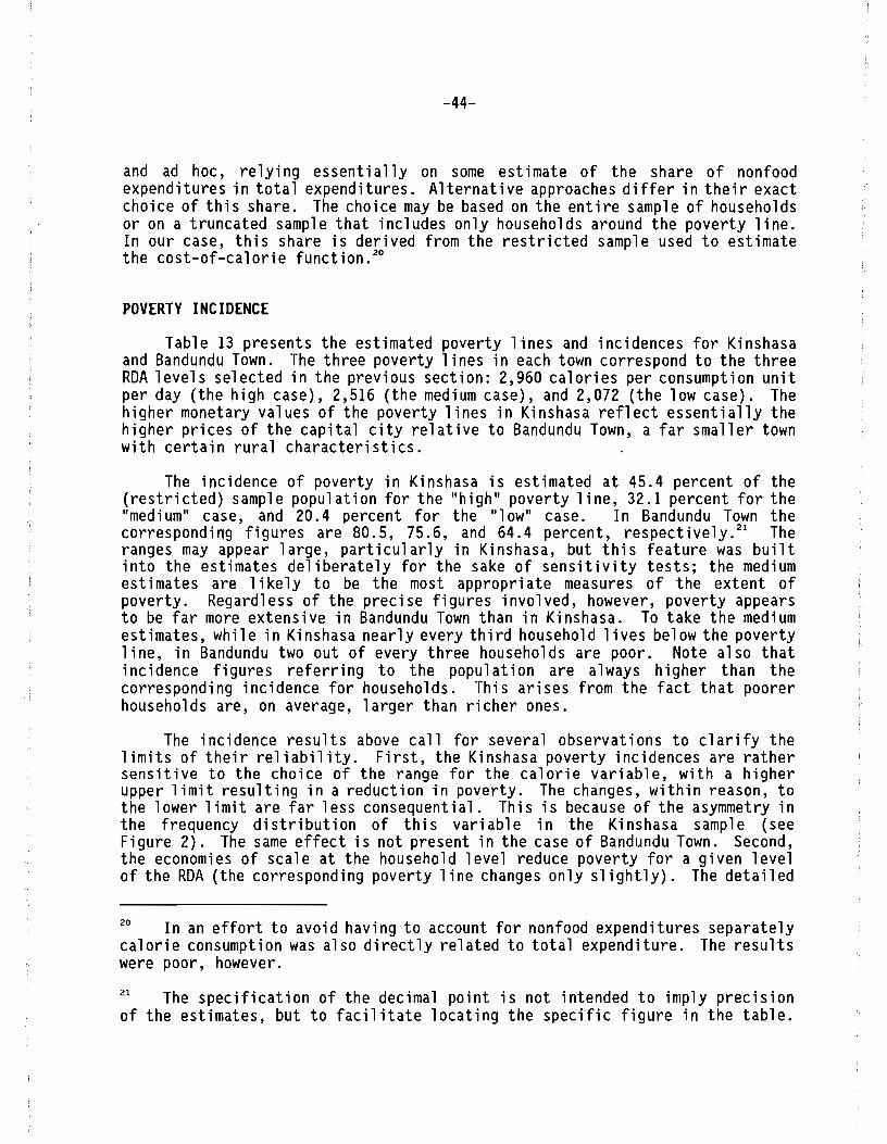
-44-

and ad hoc, relying essentially on some estimate of the share of nonfoodexpenditures in total expenditures. Alternative approaches differ in their exactchoice of this share. The choice may be based on the entire sample of householdsor on a truncated sample that includes only households around the poverty line.In our case, this share is derived from the restricted sample used to estimatethe cost-of-calorie function. 20

POVERTY INCIDENCE

Table 13 presents the estimated poverty lines and incidences for Kinshasaand Bandundu Town. The three poverty lines in each town correspond to the threeRDA levels selected in the previous section: 2,960 calories per consumption unitper day (the high case), 2,516 (the medium case), and 2,072 (the low case). Thehigher monetary values of the poverty lines in Kinshasa reflect essentially thehigher prices of the capital city relative to Bandundu Town, a far smaller townwith certain rural characteristics.

The incidence of poverty in Kinshasa is estimated at 45.4 percent of the(restricted) sample population for the "high" poverty line, 32.1 percent for the"med i urn" case, and 20.4 percent for the "low" case. In Bandundu Town thecorresponding figures are 80.5, 75.6, and 64.4 percent, respectively.21 Theranges may appear large, particularly in Kinshasa, but this feature was builtinto the estimates deliberately for the sake of sensitivity tests; the mediumest imates are 1ike1y to be the most appropri ate measures of the extent ofpoverty. Regardless of the precise figures involved, however, poverty appearsto be far more extensive in Bandundu Town than in Kinshasa. To take the mediumestimates, while in Kinshasa nearly every third household lives below the povertyline, in Bandundu two out of every three households are poor. Note also thatincidence figures referring to the population are always higher than thecorresponding incidence for households. This arises from the fact that poorerhouseholds are, on average, larger than richer ones.

The incidence results above call for several observations to clarify thelimits of their reliability. First, the Kinshasa poverty incidences are rathersensitive to the choice of the range for the calorie variable, with a higherupper limit resulting in a reduction in poverty. The changes, within reason, tothe lower limit are far less consequential. This is because of the asymmetry inthe frequency distribution of this variable in the Kinshasa sample (seeFigure 2). The same effect is not present in the case of Bandundu Town. Second,the economies of scale at the household level reduce poverty for a given levelof the RDA (the corresponding poverty line changes only slightly). The detailed

20 In an effort to avoid having to account for nonfood expenditures separatelycalorie consumption was also directly related to total expenditure. The resultswere poor, however.

21 The specification of the decimal point is not intended to imply precisionof the estimates, but to facilitate locating the specific figure in the table.

-45-

Table 13 - Kinshasa and Bandundu Town: Poverty Lines and Incidence

Kinshasa

Poverty li ne

Bandundu Town

Poverty li neSampleSize High Medium Low

SampleSize High Medium low

Poverty lines (zaires per consumptionunit per month) 790 1,143 971 799 539 697 611 521

Food 738 627 516 511 448 382Nonfood 405 344 283 186 163 139

Poverty incidencePercent of population 6,022 45.4 32.1 20.4 3,240 80.5 75.6 64.4Percent of households 790 40.6 28.0 17.5 539 73 .3 67.7 56.4

By gender of household headMale 721 41.1 27.9 17. 1 467 73.9 68.5 57.6Female 69 36.2 29.0 21.7 72 69.4 62.5 48.6

By education of household headNone 68 44.1 27.9 16.2 65 84.6 76.9 66.2Primary 272 51.1 36.4 24.6 184 83.2 78.3 67.9Secondary 383 36.3 25.6 15.1 253 67.2 61.7 49.0Higher 67 19.4 7.5 3.0 37 45.9 40.5 32.4

By socio-professional categoryof household head

Inactive and other 44 34.1 25.0 15.9 49 67.3 57.1 49.0Cadres 48 22.9 14.6 6.3 25 44.0 36.0 32.0Employees 259 39.8 31.7 20.1 168 74.4 66.7 51. 8Self-employed 186 37.1 25.8 14.5 186 76.3 72.6 60.8Skilled workers 109 46.8 25.7 16.5 65 72.3 72.3 64.6Semiskilled workers 63 57.1 36.5 23.8 16 81.3 68.8 56.3Unskilled workers 81 44.4 27.2 19.8 30 80.0 76.7 70.0

By household size1-3 members 58 13.8 8.6 5.2 126 47.6 42.1 31.04-5 147 24.4 10.9 6.1 113 73.5 62.8 48.76-7 203 39.4 27.1 15.8 147 81.0 76.9 66.08-9 189 48.7 35.4 22.8 86 84.9 81.4 72 .110 or more 193 54.4 40.4 26.4 67 89.6 86.6 76.1

-46-

empirical results are not presented here but the effect has in general been toreduce the household-level incidence by 5-10 percentage points depending on theunderlying assumptions. 22 Finally, it should be recalled that these estimatesrefer to 1985/86; the situation has almost certainly deteriorated since then.

In the context of the present discussion mention may be made of the resultsobtained by Ben-Senia (1991) for rural Bandundu. The survey was carried out inthe latter part of 1990 and the methodology used in the analysis is similar tothe one applied here. The range of RDA in his study is 2,550-3,000 for aconsumption unit and the incidence of poverty is 43-53 percent for households and50-61 percent for the population, the exact figure depending mainly on the levelof the RDA. Differences in the reference periods, the survey methods, etc., mustnot be ignored; but poverty incidence in Bandundu Town turns out to be higherthan i n rural Bandundu. It is di ffi cult to be too categori cal about thereliability of this conclusion, but it is perhaps not that surprising after all.Bandundu Town is small and characterized by many features usually found in ruralsettings. In many ways it may be thought of as a village, albeit a very largeone. For example, some 37 percent of the work force in Bandundu's two largestcities, Kikwit and Bandundu Town, is employed in agriculture23 (Shapiro 1992,p. 7). In urban Bandundu, no fewer than three out of every four independentworkers work in the agricultural sector (Shapiro 1992, p. 8) and as much as 88percent of households in Bandundu Town derive at least some income (in kind) byproducing agricultural output or livestock for their own consumption (Shapiro1992, p. 18).

The rest of Table 13 presents estimates of poverty incidence by certaincharacteristics of the household head and household size. In regard to thegender difference, female-headed households, perhaps somewhat surprisingly, donot appear to be consistently worse off than male-headed ones. In Bandundu, infact, relatively fewer households with female heads live in poverty, regardlessof the choice of the poverty line. In Kinshasa, the situation is rather morenuanced. With a high poverty 1ine, female-headed households have a sl ightlylower incidence of poverty than their male-headed counterparts, but as thepoverty line is lowered, the tables turn and households with female heads doincreasingly worse than those with male heads. This fact, in conjunction withthe addit i onal evi dence that female-headed househol ds have an average expenditurethat is as hi gh as that of male-headed ones, suggests that wh i1e the genderdifference may not matter as far as sample averages are concerned, there is moreinequality among female-headed households than among male-headed households.

22 The approach involved the estimation of household size in terms of adjustedconsumption units. The scale factors for households of various sizes (inconsumption units) were borrowed, as by Coll ier et al. (1986), from Deaton(1981).

23 The percentage is probably significantly higher in Bandundu Town, which ismuch smaller than Kikwit, Bandundu's largest town.

-47-

The level of education and the socio-professional category of the householdhead have a significant bearing on poverty status. As far as education isconcerned, the association with poverty is clearly negative, although this is notso clear cut when it comes to distinguishing between those with no education andthose with only a primary education. As regards socio-professional status, byfar the lowest poverty levels are found among households headed by cadres,regardless of the poverty line. Households with inactive heads (sans objet) dorelatively well too. The two largest groups are salaried employees and the self­employed. The first is somewhat worse off in Kinshasa than the second, but thesituation is reversed in Bandundu. Among wage workers, skill differentiationseems to lead to rather mixed results, depending on the poverty line and the townin question. The effects of skill and the level of education will be analyzedin more detail below. Finally, the positive association of poverty withhousehold size comes out unambiguously from the results at the bottom of thetable, a conclusion that was already reached above from the fact that incidenceof poverty in the population was higher than among the households. In Kinshasahouseholds with 10 or more members have an incidence of poverty which is four tofive times higher than that for households with up to three members. In BandunduTown the disparity is less, about twice as high.

POVERTY PROFILES

Tables 14 and 15 report the decomposition of poverty by several character­istics of the household or of its head. The index Pz represents, in both Fosteret al. (FGT) and Ray forms, the severity of poverty-and can only be interpretedrelative to its average value or to the values referring to other groups. Itsabsolute value has no significance as such. According to the FGT index, povertyin Kinshasa is more severe for male-headed households than for female-headed oneseven though the incidence of poverty is slightly higher among the latter. As aresult, the contribution of the former to total poverty, 92.1 percent, issomewhat larger than its share of households in the sample, 91.3 percent. Thiscontrast points to the value of a more complete index of poverty than the simpleheadcount ratio. The Ray index conveys the same story.

When Kinshasa households are grouped according to the level of education ofthe household head, all three indices - the poverty incidence and the FGT andRay indices - point in the same direction: poverty is highest and most severeamong those with a primary education and lowest and least severe among those withmore education. More than half of total poverty is attributable to thosehouseholds whose heads have a primary education although they constitute onlyjust over a third of the sample. Similarly, semiskilled workers are the mostaffected group among the various socio-professional groupings and cadres are theleast affected. As far as household size is concerned, all three indicators riseuniformly, with the level and severity of poverty increasing as household sizegrows. Furthermore, it should be noted that all these results are based on thesample of households, not individuals. If individuals were to be the unit ofanalysis, both the levels and the severity of poverty would be still more to the

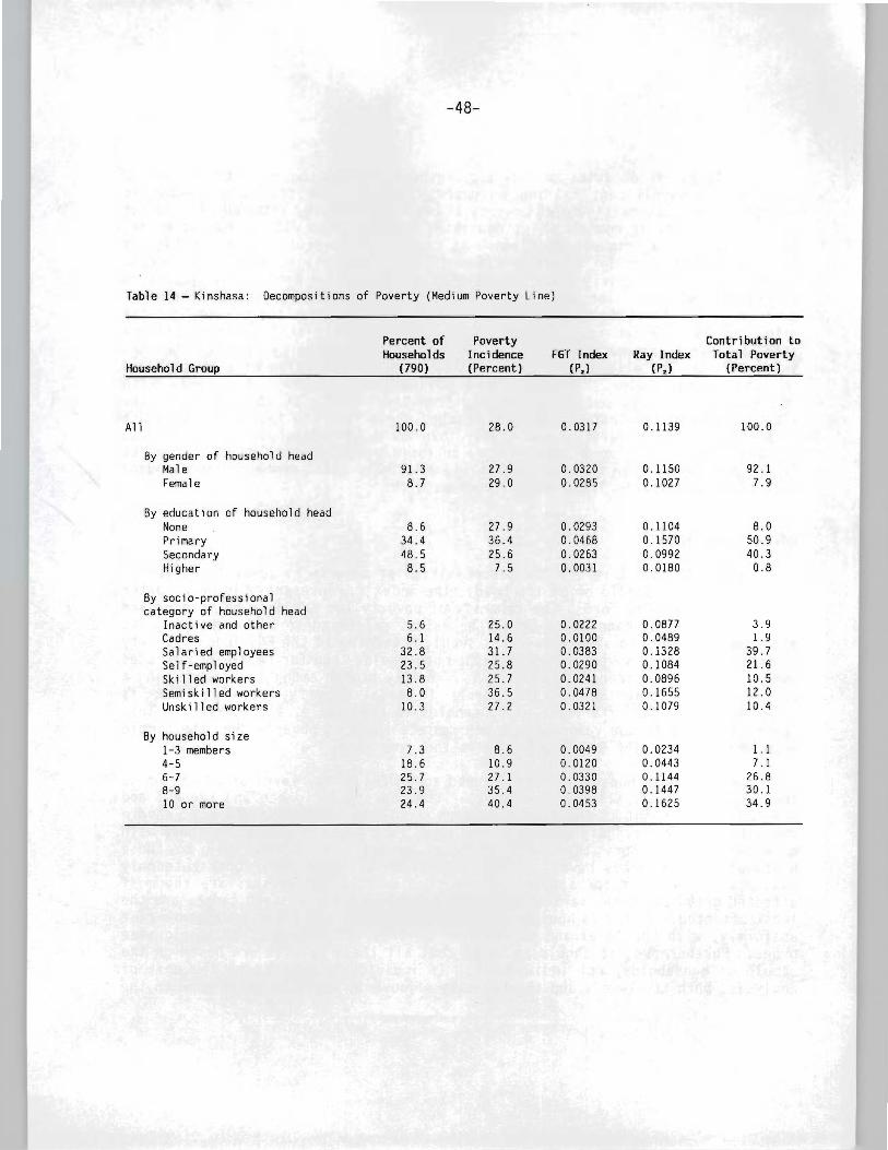
-48-

Table 14 - Kinshasa: Decompositions of Poverty (Medium Poverty Line)

Household Group

Percent ofHouseholds

(790)

PovertyIncidence(Percent)

FGT Index(P,)

Ray Index(P,)

Contribution toTotal Poverty

(Percent)

All 100.0 28.0 0.0317 0.1139 100.0

8y gender of household headMale 91.3 27.9 0.0320 0.1150 92.1Female 8.7 29.0 0.0285 0.1027 7.9

By education of household headNone 8.6 27.9 0.0293 0.1104 8.0Primary 34.4 36.4 0.0468 0.1570 50.9Secondary 48.5 25.6 0.0263 0.0992 40.3Higher 8.5 7.5 0.0031 0.0180 0.8

By socio-professionalcategory of household head

Inactive and other 5.6 25.0 0.0222 0.0877 3.9Cadres 6.1 14.6 0.0100 0.0489 1.9Salaried employees 32.8 31.7 0.0383 0.1328 39.7Self-employed 23.5 25.8 0.0290 0.1084 21.6Sk ill ed workers 13.8 25.7 0.0241 0.0896 10.5Semiskilled workers 8.0 36.5 0.0478 0.1655 12.0Unskilled workers 10.3 27.2 0.0321 0.1079 10.4

By household size1-3 members 7.3 8.6 0.0049 0.0234 1.14-5 18.6 10.9 0.0120 0.0443 7. 16-7 25.7 27.1 0.0330 0.1144 26.88-9 23.9 35.4 0.0398 0.1447 30.110 or more 24.4 40.4 0.0453 0.1625 34.9

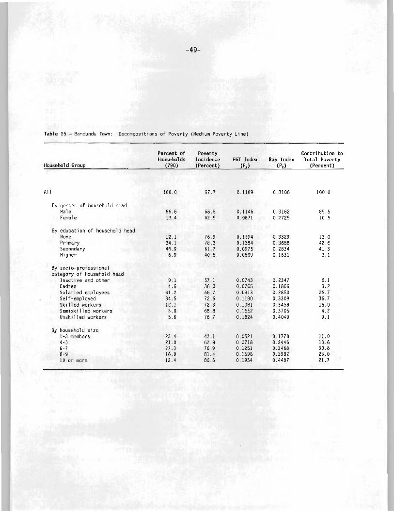
-49-

Table 15 - Bandundu Town: Decompositions of Poverty (Medium Poverty Line)

Household Group

Percent ofHouseholds

(790)

PovertyIncidence(Percent)

FGT Index(P.)

Ray Index(P.)

Contribution toTotal Poverty

(Percent)

All 100.0 57.7 0.1109 0.3106 100.0

By gender of household headMale 85.5 58.5 0.1145 0.3152 89.5Female 13.4 52.5 0.0871 0.2725 10.5

By education of household headNone 12. I 75.9 0.1194 0.3329 13.0Primary 34.1 78.3 0.1384 0.3688 42.5Secondary 46.9 61. 7 0.0975 0.2834 41.3Higher 5.9 40.5 0.0509 0.1531 3.1

By socio-professionalcategory of household head

Inactive and other 9.1 57.1 0.0743 0.2347 6.1Cadres 4.6 36.0 0.0765 0.1866 3.2Salaried employees 31.2 66.7 0.0913 0.2850 25.7Self-employed 34.5 72.6 0.1180 0.3309 36.7Sk ill ed worke,rs 12.1 72.3 0.1381 0.3458 15.0Semiskilled workers 3.0 68.8 0.1552 0.3705 4.2Unskilled workers 5.6 76.7 0.1824 0.4049 9.1

By household size1-3 members 23.4 42.1 0.0521 0.1770 11. 04-5 21.0 62.8 0.0718 0.2446 13.66-7 27.3 76.9 0.1251 0.3468 30.88-9 16.0 81.4 O. 1598 0.3982 23.010 or more 12.4 86.6 0.1934 0.4487 21.7

-50-

disadvantage of the larger households since, as we saw in Table 13, povertyincidence is higher among individuals than among households.

The situation in Bandundu Town may be similarly analyzed. Briefly, male­headed households come out worse off than female-headed ones regardless of theindicator; the contrast noted in the case of Kinshasa between the incidence andseverity of poverty is not present here. Another noteworthy difference comparedto Kinshasa is that among socio-professional groups in Bandundu Town, theunskilled workers are worse off than the semiskilled ones, but cadres do besthere as well. The effect of household size is the same as in Kinshasa.

Finally, the rankings of groups obtained from the FGT and Ray indices areusually the same, but not always; differences may be seen, for instance, in acomparison of the self-employed and the unskilled workers in Kinshasa.

MULTIVARIATE ANALYSIS

The analysis so far has been concerned with the association of poverty witha number of characteristics of the household or of its head one at a time. Wewill now consider the possible joint effects of these characteristics. With amultivariate analysis we can begin to discern the individual effect of each inthe presence of others, a situation resembling the real world.

The basic issue is the identification of factors that independently affecthousehold income or expenditure. For this purpose a number of regressionequations were estimated with the logarithm of total household expenditures perconsumption unit as the dependent variable and the following as independentvariables: household size (in both consumption units and number of members),educational attainment of the household head (represented as a continuousvariable with the number of years of schooling), the sex of the household head(as a dummy variable), and the socio-professional category of the household head(dummy variables distinguishing among wage-earning workers, independent workers,and the rest). Some specifications also included interaction terms among pairsof the following three variables: education, sex, and socio-professionalcategory of the household head. In each of the two cities under consideration,the regressions were run on both the full samples of households and therestricted samples used to derive the poverty profiles.

Table 16 presents some typical results, using the simplest specifications.The most important point to emphasize is that the size of the household and theeducational level and sex of its head are statistically highly significant (at1 percent level) in both Kinshasa and Bandundu Town. This suggests that each ofthese three vari abl es has an effect that is independent of the other two.Household size is negatively associated with total expenditures per consumptionunit, but is positively associated with the level of education of the householdhead. The positive sign of the sex dummy indicates that, when the effects ofother included variables are accounted for, female-headed households have ahigher expenditure level than male-headed ones, an interesting result. The dummyvariables relating to the socio-professional category of the household head are,

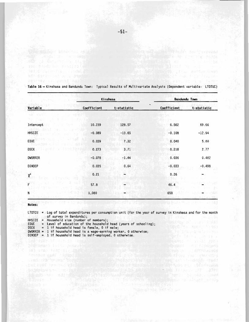
-51-

Table 16 - Kinshasa and Bandundu Town: Typical Results of Multivariate Analysis (Dependent variable: LTOTUC)

Kinshasa Bandundu Town

Variable Coefficient t-statistic Coefficient t-statistic

Intercept

HHSIZE

EDUC

DSEX

DWORKER

DINDEP

F

N

Notes:

LTOTCU

HHSIZEEDUCDSEXDWORKER =DINDEP =

10.239 128.57 6.562 69.66

-0.089 -13.65 -0.108 -12.94

0.039 7.32 0.040 5.80

0.273 3.71 0.218 2.77

-0.078 -1.44 0.036 0.482

0.035 0.64 -0.033 -0.498

0.21 0.26

57.8 46.4

1,080 650

Log of total expenditures per consumption unit (for the year of survey in Kinshasa and for the monthof survey in Bandundu);Household size (number of members);Level of education of the household head (years of schooling);1 if household head is female, 0 if male;1 if household head is a wage-earning worker, 0 otherwise;1 if household head is self-employed, 0 otherwise.

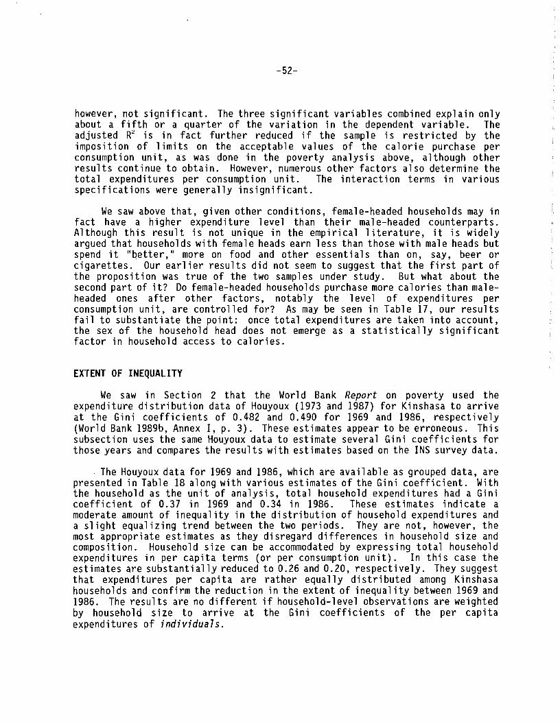
-52-

however, not significant. The three significant variables combined explain onlyabout a fifth or a quarter of the variation in the dependent variable. Theadjusted R2 is in fact further reduced if the sample is restricted by theimposition of limits on the acceptable values of the calorie purchase perconsulllpt i on un it, as was done in the poverty anal ys is above, although otherresults continue to obtain. However, numerous other factors also determine thetotal expenditures per consumption unit. The interaction terms in variousspecifications were generally insignificant.

We saw above that, given other conditions, female-headed households may infact have a hi gher expenditure 1eve1 than thei r male-headed counterparts.Although this result is not unique in the empirical 1iterature, it is widelyargued that households with female heads earn less than those with male heads butspend it "better," more on food and other essentials than on, say, beer orcigarettes. Our earlier results did not seem to suggest that the first part ofthe proposition was true of the two samples under study. But what about thesecond part of it? Do female-headed households purchase more calories than male­headed ones after other factors, notably the level of expenditures perconsumption unit, are controlled for? As may be seen in Table 17, our resultsfail to substantiate the point: once total expenditures are taken into account,the sex of the household head does not emerge as a statistically significantfactor in household access to calories.

EXTENT OF INEQUALITY

We saw inSect ion 2 that the Worl d Bank Report on poverty used theexpenditure distribution data of Houyoux (1973 and 1987) for Kinshasa to arriveat the Gini coefficients of 0.482 and 0.490 for 1969 and 1986, respectively(World Bank 1989b, Annex I, p. 3). These estimates appear to be erroneous. Thissubsection uses the same Houyoux data to estimate several Gini coefficients forthose years and compares the results with estimates based on the INS survey data.

The Houyoux data for 1969 and 1986, which are available as grouped data, arepresented in Table 18 along with various estimates of the Gini coefficient. Withthe household as the unit of analysis, total household expenditures had a Ginicoefficient of 0.37 in 1969 and 0.34 in 1986. These estimates indicate amoderate amount of inequality in the distribution of household expenditures anda slight equalizing trend between the two periods. They are not, however, themost appropriate estimates as they disregard differences in household size andcomposition. Household size can be accommodated by expressing total householdexpenditures in per capita terms (or per consumption unit). In this case theestimates are substantially reduced to 0.26 and 0.20, respectively. They suggestthat expenditures per capita are rather equally distributed among Kinshasahouseholds and confirm the reduction in the extent of inequality between 1969 and1986. The results are no different if household-level observations are weightedby household size to arrive at the Gini coefficients of the per capitaexpenditures of individua7s.

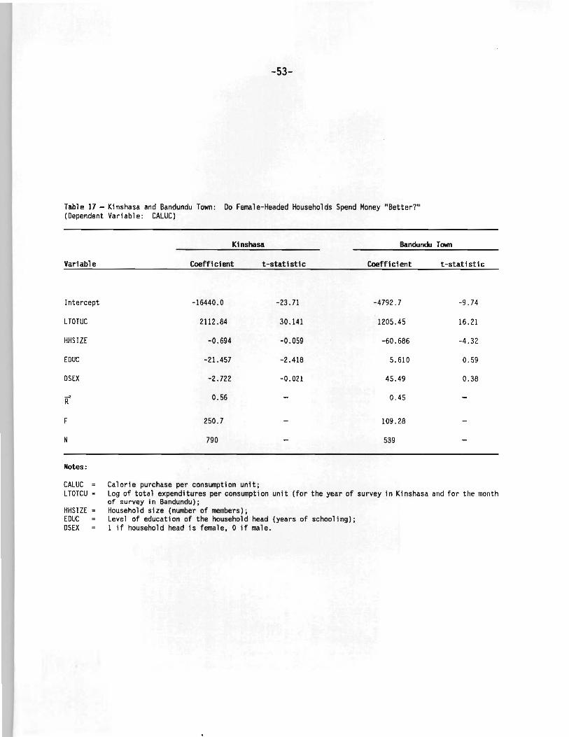
-53-

Table 17 - Kinshasa and Bandundu Town: Do Female-Headed Households Spend Money "Better?"(Dependent Variable: CALUC)

Kinshasa Bandundu Town

Variable Coefficient t-statistic Coefficient t-statistic

Intercept

LTDTUC

HHSIZE

EDUC

DSEX

F

N

Notes:

CALUCLTOTCU =

HHSIZEEDUCDSEX

-16440.0 -23.71 -4792.7 -9.74

2112.84 30.141 1205.45 16.21

-0.694 -0.059 -60.686 -4.32

-21. 457 -2.418 5.610 0.59

-2.722 -0.021 45.49 0.38

0.56 0.45

250.7 109.28

790 539

Calorie purchase per consumption unit;Log of total expenditures per consumption unit (for the year of survey in Kinshasa and for the monthof survey in Bandundu);Household size (number of members);Level of education of the household head (years of schooling);1 if household head is female, 0 if male.

Table 18 - Kinshasa: Distribution of Expenditures Among Expenditure Groups, 1969 and 1986

Expenditure per Expenditure per Expendi ture perHousehold Capita Household Size Consumption Unit

110. of 110. of Household Size (zaires per (zaires per (conslDption (zaires perAverage Household Expenditures Households Menmers (Menmers) IOI'lth) month) units) month)(zai res per IIIonth) (1) (2) (3) (4) (5) (6) (7)

19691. Less than 15 298 1,331 4.47 10.96 2.45 3.16 3.472. 15 - < 20 259 1,340 5.17 17.63 3.41 3.71 4.753. 20 - < 25 261 1,515 5.80 22.49 3.87 4.16 5.414. 25 - < 35 273 1,626 5.96 29.25 4.91 4.23 6.915. 35 - < 60 240 1,648 6.87 44.51 6.48 4.93 9.036. 60 and more 140 1,171 8.36 99.04 11.84 5.97 16.59

Total 1,471 8,631 5.87 31.43 5.36 4.19 7.50

19861. Less than 4,000 34 143 4.2 3,105 739 I

U'12. 4,000 - < 5,250 34 228 6.7 4,649 694 ~

3. 5,250 - < 6,500 35 235 6.7 5,850 873 I

4. 6,500 - < 8,000 33 241 7.3 7,131 9775. 8,000 - < 13,000 35 298 8.5 10,046 1,1826. 13,000 and more 34 357 10.5 20,912 1,992

Total 205 1,502 7.3 8,563 1,173

Gini Coefficients, Grouped Data 1969 1986

Total expenditure per household (household sample) 0.37 0.34Total expenditure per capita (household sample) 0.26 0.20Total expenditure per consumption unit

(household sample) 0.26Total expenditure per capita (weighted by

household size) 0.27 0.21Total expenditure per consumption unit (weighted by

household size) 0.27

Source: For 1969, Houyoux (1973), p. 107 for items 1 and 4, p. 51 for item 2 and p. 108 for item 6; for 1986, Houyoux (1987), p. AS1 for items1, 3 and 4. Other columns can be easily derived.

-55-

The reduction in expenditure "inequal ity is generally attributed to thephenomenon of dualisme culturel (see Section 2) whereby better-off families opentheir homes to the less fortunate members of the extended family in times ofeconomic distress. Notwithstanding its estimates of the Gini coefficient and theaccompanying Lorenz curves, which indicated a deterioration in the expendituredistribution, the World Bank Report also examined the expenditure differentialsamong income groups. The Report concl udes that incomes tended to 1eve1 offbetween 1969 and 1986. This evidence "seems to confirm the hypothesis that oneof the by-products of the deteriorating economic environment has been the higherlevels of migration within Kinshasa to wealthier households (or from rural areasto visit relatives in Kinshasa), rather than a dramatic increase in overallpoverty levels in the capital" (World Bank 1989b, Annex I, p. 6, emphasis in theoriginal).

We saw that expenditures per capita appear to be rather equally distributedin Kinshasa. But the relevant Gini coefficients are subject to a downward biaswhose extent is not readily determi ned. The fi rst source of bi as is theunderreporting of expenditures, which tends to be considerably greater among thericher households than among the poorer ones. This is a perennial problem inhousehold surveys and leads to an underestimation of the extent of inequality.A second source of downward bi as is the use of ~rouped data, whi ch removeswithin-group variations in the averaging process. 2 The latter does not arisefrom the expenditure data from the INS surveys, which are available forindividual households. The estimated Gini coefficients of expendituredistribution for 1985/86 based on the INS data are presented in Table 19 forKinshasa and Bandundu Town.

The results in Table 19, and their comparison with those in Table 18, permitseveral observations. First, the Gini coefficient of the distribution ofhousehold expenditures in Kinshasa is 0.40. This estimate, which refers to1985/86, is somewhat larger than the downward-biased estimate for 1986 based onHouyoux's grouped data (0.34). If the samples were comparable, the differencecould be essentially attributed to the effect of grouping. Secondly, householdexpenditures per capita or per consumption unit are distributed slightly moreunequally than household expenditures, despite the positive association betweenexpenditures and household size. This finding stands in contrast with theearlier result based on the Houyoux data for 1986 where the Gini coefficientdropped sharply from 0.34 to 0.20 as a result of the conversion of expendituresinto per capita terms. This contrast points to the pitfalls of using groupeddata to estimate inequality indices. Thirdly, food expenditures are, as mightbe expected, more equally distributed than total expenditures for correspondingdefinitions of the expenditure variable. Finally, the extent of inequality inBandundu Town is much the same as in Kinshasa for all variables. The greaterpoverty in the former town is therefore ent ire1y due to its lower 1eve1 ofaverage income and expenditure relative to Kinshasa.

24 The use of expenditure data also tends to understate income inequality,which is normally greater than expenditure inequality.

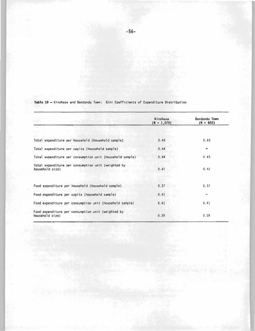
-56-

Table 19 - Kinshasa and Bandundu Town: Gini Coefficients of Expenditure Distribution

Kinshasa(M = 1,079)

Bandundu Town(M = 650)

Total expenditure per household (household sample) 0.40 0.40

Total expenditure per capita (household sample) 0.44

Total expenditure per consumption unit (household sample) 0.44 0.45

Total expenditure per consumption unit (weighted byhousehold size) 0.41 0.42

Food expenditure per household (household sample) 0.37 0.37

Food expenditure per capita (household sample) 0.41

Food expenditure per consumption unit (household sample) 0.41 0.41

Food expenditure per consumption unit (weighted byhousehold size) 0.39 0.39

1"'1 /_ '7

6. CONCLUSIONS

The economy of Zaire has been going through a deepening crisis for at leasta decade. Various attempts at stabilization and structural adjustment, whichwere never seriously pursued, have failed to stop the rapid deterioration, andthe problem is now compounded by the paralysis of the political process. Theinternational financial agencies have virtually abandoned the country to itsfate, pending the outcome of the political crisis. And, obviously, no seriousinitiatives may be expected from either of the two parallel governments thatcurrently "run" the country to put the economic house in order. Under thesecircumstances, the poverty-stricken people in Zaire are likely to face evenharder days ahead in their struggle to survive.

This study focused on determining the poverty profiles of Kinshasa, thecapital city, and Bandundu Town, a town with a population of about 60,000 in theneighboring Bandundu region. The main data came from two household surveyscarried out by the INS in 1985/86. Although the samples were reasonably largefor the purpose, the analysis was hampered occasionally by the poor quality ofthe data, and the results must accordingly be treated with caution.

The main findings may be summarized as follows. The incidence of povertyin Kinshasa is estimated at about a third of the population as of the mid-1980s.This level, which is based on a "medium" poverty line, is likely to haveincreased substantially since then as a result of the deteriorating economicsituation. Poverty in Bandundu Town is estimated to have been much higher,affecting as much as three-quarters of the population.

Several household characteristics are found to be significantly associatedwith poverty in both cities. Households with younger and better educated headstend to be less poor than those headed by older people with less education. Thesocio-professional status of the household head is also associated with poverty,with the lowest poverty being found among households headed by cadres and thehighest poverty among manual and semiskilled workers. Household size is thevariable that is most significantly (and positively) related to poverty:Kinshasa households with 10 or more members have an incidence of poverty four tofive times higher than that for households with up to 3 members. The correspond­ing disparity in Bandundu Town is less marked, about twice as high. Householdswith different income levels inhabit all types of neighborhoods in both citiesbut, on the whole, "residential areas" tend to be populated by the richerhouseholds and extension areas by the poorer ones.

The gender of the household head is also found to be associated with povertyin both cities but in a rather surprising direction: female-headed householdshave on average higher "incomes and lower poverty incidence than male-headedhouseholds. This is true at all levels of the poverty line in Bandundu Town but

-58-

becomes less pronounced and is eventually reversed in Kinshasa with the loweringof the poverty threshold. Even then, however, the severi ty of poverty, asmeasured by the FGT and Ray indices, remains higher for male-headed than forfemale-headed households. The argument that, for a given level of resources,female-headed households tend to spend relatively more on essentials, such asfood, than male-headed households is not supported by our empirical results.

Finally, based on grouped data from other surveys, estimates of the Ginicoefficient of expenditure distribution reveal a certain reduction in the extentof inequal ity in Kinshasa between 1969 and 1986, an improvement that isattributed to the opening up of the richer households to the poorer members oftheir extended families as economic conditions deteriorated. On the basis ofungrouped data from the INS surveys, however, the extent of inequality is foundto be rather significant, with Gini coefficients of approximately 0.40 in bothKinshasa and Bandundu Town.

-59-

APPENDIXAXIOMATIC APPROACH TO THE CONSTRUCTION OF POVERTY INDICES:

A REVIEW

The headcount ratio is the simplest aggregate measure of the extent ofpoverty in a population of individuals or households. It is also the leasti nformat i ve for it captures no more than the proport i on of the poor in thepopulation. It may be expressed as:

H = q/n, (6)

where q is the number of the poor and n is the total population.

Among the shortcomings of the headcount index (and there are several) is itsinsensitivity to how poor the poor are, i.e., the extent to which their incomes(or expenditures) fall short of the poverty 1ine.. There is a measure thatcaptures this dimension of poverty. It relies on the notion of the poverty gapof a poor individual, which is defined as:

(7)

where z is the poverty line and Y1 is the income of individual i. These gaps maybe expressed as proportions of the poverty line (common to all individuals) andaveraged over all poor individuals to arrive at the so-called poverty gap ratio:

q

I = (l/q) L g)z = g/z,i -1

-where g is the "mean poverty gap."

(8)

As a stand-alone poverty index, the poverty gap ratio suffers itself fromthe serious shortcoming of being insensitive to the proportion of the poor in thepopulation. It is therefore more appropriately viewed as a complement to theheadcount ratio than as a substitute for it. Some empirical studies, therefore,report both H and I side by side (see, for example, Chan 1990). This has theinconvenience of making intergroup and interternporal comparisons difficult. Asingle index is generally preferable, and a substantial and growing literatureis devoted to the construction of different indices that combine variousproperties commonly viewed as being desirable. These properties are normallyformulated as axioms.

The axiomatic approach to the construction of poverty indices was pioneeredby Sen (1976, 1979). He formulated two appealing axioms:

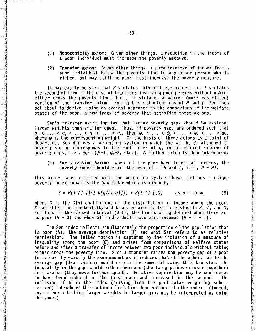
-60-

where G is the Gini coefficient of the distribution of income among the poor.S satisfies the monotonicity and transfer axioms, is increasing in H, I, and G,and lies in the closed interval (0,1), the limits being defined when there areno poor (H = 0) and when all individuals have zero incomes (H = I = 1).

The Sen index reflects simultaneously the proportion of the population thatis poor (H), the average deprivation (1) and what Sen refers to as relativedeprivation. The latter notion is captured by the inclusion of a measure ofinequality among the poor (G) and arises from comparisons of welfare statesbefore and after a transfer of income between two poor individuals without makingeither cross the poverty line. Such a transfer raises the poverty gap of a poorindividual by exactly the same amount as it reduces that of the other. While theaverage gap (deprivation) would remain the same following this transfer, theinequality in the gaps would either decrease (the two gaps move closer together)or increase (they move further apart). Relative deprivation may be consideredto have been reduced in the fi rst case and increased in the second. Theinclusion of G in the index (arising from the particular weighting schemederived) introduces this notion of relative deprivation into the index. (Indeed,any scheme attaching larger weights to larger gaps may be interpreted as doingthe same.)

(9)as q ---) 00,S = H(l-(l-I)(l-G[qj(l+q)]}) = H[I+(l-I)G]

(1) Monotonicity Axiom: Given other things, a reduction in the income ofa poor individual must increase the poverty measure.

(2) Transfer Axiom: Given other things, a pure transfer of income from apoor individual below the poverty line to any other person who isricher, but may still be poor, must increase the poverty measure.

It may easily be seen that Hviolates both of these axioms, and I violatesthe second of them in the case of transfers involving poor persons without makingeither cross the poverty line, i.e., it violates a weaker (more restricted)version of the transfer axiom. Noting these shortcomings of H and I, Sen thenset about to derive, using an ordinal approach to the comparison of the welfarestates of the poor, a new index of poverty that satisfied these axioms.

Sen's transfer axiom implies that larger poverty gaps should be assignedlarger weights than smaller ones. Thus, if poverty gaps are ordered such that91 ~ ••• ~ 9j ~ ••• ~ 9k ~ ••• ~ 9q , then <PI ~ ••• ~ <Pj ~ ••• ~ <Pk ~ ••• ~ <Pq '

where <P is the corresponding weight. On the basis of three axioms as a point ofdeparture, Sen derives a weighting system in which the weight <Pi attached topoverty gap 9i corresponds to the rank order of 9; in an ordered ranking ofpoverty gaps, i.e., <p;=i (<P1=1, <p2=2, etc.). A further axiom is then introduced:

(3) Normalization Axiom: When all the poor have identical incomes, thepoverty index should equal the product of H and I, i.e., P = HI.

This axiom, when combined with the weighting system above, defines a uniquepoverty index known as the Sen index which is given by:

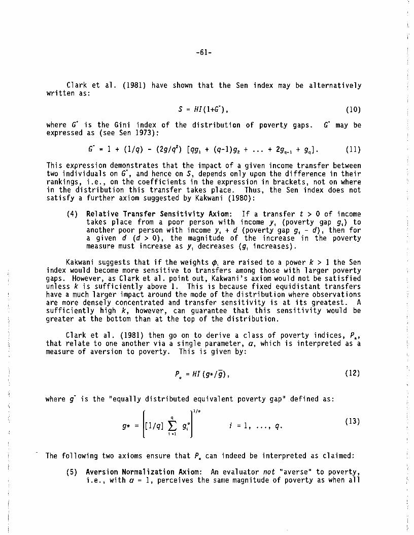
-61-

Clark et al. (1981) have shown that the Sen index may be alternativelywritten as:

S = HI(l+Go), (10)

where GO is the Gini index of the distribution of poverty gaps. GO may beexpressed as (see Sen 1973):

GO = 1 + (l/q) - (2g/qZ) [qgl + (q-l)gz + ... + 2gq_1 + gq]' (11)

This expression demonstrates that the impact of a given income transfer betweentwo individuals on GO, and hence on S, depends only upon the difference in theirrankings, i.e., on the coefficients in the expression in brackets, not on wherein the distribution this transfer takes place. Thus, the Sen index does notsatisfy a further axiom suggested by Kakwani (1980):

(4) Relative Transfer Sensitivity Axiom: If a transfer t > 0 of incometakes pl ace from a poor person with income Yi (poverty gap gil toanother poor person with income Yi + d (poverty gap gi - d), then fora given d (d > 0), the magnitude of the increase in the povertymeasure must increase as Yi decreases (gj increases).

Kakwani suggests that if the weights ¢i are raised to a power k > 1 the Senindex would become more sensitive to transfers among those with larger povertygaps. However, as Clark et al. point out, Kakwani's axiom would not be satisfiedunless k ;s sufficiently above 1. This is because fixed equidistant transfershave a much larger impact around the mode of the distribution where observationsare more densely concentrated and transfer sensitivity is at its greatest. Asufficiently high k, however, can guarantee that this sensitivity would begreater at the bottom than at the top of the distribution.

Clark et al. (1981) then go on to derive a class of poverty indices, p.,that relate to one another via a single parameter, G, which is interpreted as ameasure of aversion to poverty. This is given by:

where g is the "equally distributed equivalent poverty gap" defined as:

(I2)

i =1, ... , q. (13)

- The following two axioms ensure that p. can indeed be interpreted as claimed:

(5) Aversion Normalization Axiom: An evaluator not "averse" to poverty,i.e., with G = 1, perceives the same magnitude of poverty as when all

-62-

where w. > 0 is the weight attached to the poverty of subgroup j and m is thenumber ~f subgroups. Anew class of poverty indices that does have this propertyis that introduced by Foster, Greer, and Thorbecke (1984), which is written asfollows:

(14)

(15)

(16)a ~ O.

q

Po = (lin) L ([z -Y;l/zt;1 -I

q

Po = (lIn) L (g;l zri -1

poverty gaps are equal, i.e., PI (with all gj'S equal) = HI, where itis assumed that (3) holds.

(6) Aversion Normalization Axiom: p. increases monotonically with a, i.e.,the more "averse" one is to poverty, the greater does he perceive thelevel of poverty to be, all other things being constant.

The above poverty indices lack an essential property in the generation ofpoverty profiles, namely, decomposability. A poverty index is said to be"additively decomposable" if:

or,

Two further axioms relate to this class of poverty indices:

(7) Weak Additive Decomposability Axiom: The weights, w~, vary directlywith the subgroup's population share, njln, where nj 1S the number ofindividuals in the subgroup and n = L nj is the total population; inother words, the larger the population share, the greater the impactof a rise in subgroup poverty.

(8) Strong Additive Decomposability Axiom: The weights, wj ' vary directlywith the subgroup's "mean poverty gap" relative to that for the wholepopulation; in other words, ceteris paribus, the poorer a subgroup'spoor are on average, the greater the impact of a ri se in thatsubgroup's poverty on aggregate poverty.

A final axiom, introduced by Ray (l989) , seeks to combine the "povertyaversion" notion in the Clark et al. approach with the "additive decomposability"of the Foster, Greer, and Thorbecke poverty measure:

-63-

(9) Addit; ve Decomposabil ity and Avers; on Monoton; city Ax; om: p. wi 11satisfy this axiom if it can be written as:

W. P. ,J.Q J.Q(17)

where the subgroup poverty indices, Pj ., increase with a, while the correspondingwe i ghts, wj ,.' increase with a for subgroups with "above average" poverty, anddecrease for those with "below average" poverty; moreover, in keeping with thespirit of "poverty aversion" and axiom (6) above, p. itself must increase witha.

Ray (1989) notes that of those poverty indices mentioned above, nonesatisfies all of the nine axioms: the Sen index violates (4), among others; thatby Clark et al. violates (7) to (9); and the Foster, Greer, and Thorbecke indexviolates (5), (6), and (9). Ray proposes an alternative measure given by:

q

PQ

= (g/nz) L (9J9 r,i .. 1

(18)

where 9 is the "mean poverty gap." This measure satisfies a77 of the nine axioms(for proof, see Ray 1989). It may easily be shown that for a = 2 the contribu­tion of each subgroup to total poverty is the same in the Ray index as in theFoster et al. (1984) index.

This study uses the headcount ratio, the Foster et al. index, and the Rayindex. For a discussion of the relationships among these three indices, seeSection 3.

-64-

REFERENCES

Ben-Senia, Mohamed. 1991. Agricultural Production, Poverty and Consumption inRural Bandundu. Paper prepared for the research project on the Impact ofStructural Adjustment on Low-income Population Groups in Zaire, CornellUniversity Food and Nutrition Policy Program. September. Mimeographed.

Chan, Elaine K. 1990. ACompendium of Data on Poverty and Income Distribution.Background paper for the World Development Report. Washington, D.C.:World Bank. Mimeographed.

Clark, Stephen, Richard Hemming, and David Ulph. 1981. liOn Indices for theMeasurement of Poverty." In Economic Journal. 91 (June): 515-526.

Collier, Paul, Samir Radwan, Samuel Wangwe (with Albert Wagner). 1986. Labourand Poverty in Rural Tanzania. Oxford: Clarendon Press.

Cour, Jean-Marie. NO. The Unrecorded Economy in Zaire and Its Contribution tothe Real Economy.

Deaton, Angus. 1981. Three Essays on a Sri Lanka Household Survey. LSMSWorking Paper No. 11. Washington, D.C.: World Bank.

Drosin, J.A. 1988. Combatting Malnutrition in Urban Kinshasa. USAID/ORT Foodfor Peace PL480, Title II, MCH Project. Mimeographed.

Foster, James, Joel Greer, and Erik Thorbecke. 1984. "A Class of DecomposablePoverty Measures." Econometrica. 52(3): 761-766.

Food and Agriculture Organization. 1957. Besoins en Calories. Rome: FAO.

1987. The Fifth World Food Survey. Rome: FAO.

Greer, Joel, and Erik Thorbecke. 1986. Food Poverty and Consumption Patternsin Kenya. Geneva: ILO.

Houyoux, C., and J. Houyoux. 1970. ilLes conditions de vie dans soixantefamilles ~ Kinshasa." In Cahiers Economiques et Sociaux, Vol. VIII, No.1,Mars. (Institut de Recherches Economiques et Sociales (IRES), UniversiteLovanium, Kinshasa.)

Houyoux, Joseph. 1971. Resultats partiels de l'enquete sur les conditions devie ~ Kinshasa. Mimeographed.

__.,.,........--,-. 1973. Budgets menagers, nutrition et mode de vie a Kinshasa.Kinshasa: Presses Universitaires du Zaire.

-65-

1986. Consommation des produits vivriers a Kinshasa et dans lesgrandes vi7les du Zaire. ICHEC (Bruxelles) and BEAU (Bureau d'Etudesd'Amenagement et d'Urbanisme, Kinshasa).

____________ . 1987. Budgets menagers. Annex B in BEAU et la Banque Mondiale.

INS (Institut National de la Statistique - Zaire). 1984. Projet Enquete BudgetConsommation des Menages: Manuel d'enqueteur. Kinshasa: INS. Mimeo­graphed.

1989a. Enquete budgets menagers: Principaux resultatsBandundu, 1985. Kinshasa: INS.

Vi7lede

1989b. Enquete budgets menagers: Principaux resultats -- Ville deKinshasa, 1985. Kinshasa: INS.

1989c. Quantite reelle consomee par personne et par mois: Villede Kinshasa, EBCM - 1985. Kinshasa: INS. Mimeographed.

1989d. Quantite reelle consomee par personne et par mois: Villede Bandundu, EBCM - 1985. Kinshasa: INS. Mimeographed.

1990. Resultats du programme de revision des comptes nationaux auZaire. Kinshasa: INS. Mimeographed.

Kalisa, M. 1989. Programme d'aide alimentaire canadienne en relation avec lasituation alimentaire au Zaire. Kinshasa: Centre de Cooperation Zaire­Canada. Kinshasa.

Kalonji, Ntalaja, Sita Lumbuenamo, and Kashoba Ngelengwa. 1991. Consommationalimentaire, etat nutritionnel et pauvrete dans les Villes de Kinshasa etde Bandundu: Revue de litterature. Paper prepared for the research projecton the Impact of Structural Adjustment on Low-income Population Groups inZaire, Cornell University Food and Nutrition Policy Program. Mimeographed.

Kakwani, N. 1980. "On a Class of Poverty Measures." Econometrica. 48(March): 437-446.

Kyereme, Stephen S., and Eri k Thorbecke. 1987. "Food Poverty Prof; 1e andDecomposition Applied to Ghana." World Development. 15(9): 1189-1199.

Latham, M.C. 1965. Human Nutrition in Tropical Africa. Rome: FAO.

Maton, Jef. 1992. How do the Poor in Kinshasa Survive: Miracle, Enigma orBl ack Box? Paper prepared for the research project on the Impact ofStructural Adjustment on Low-income Population Groups in Zaire, CornellUniversity Food and Nutrition Policy Program. March. Mimeographed.

-66-

MacGaffey, Janet. 1983. "How to Survive and Become Rich Amidst Devastation:The Second Economy in Zaire." African Affairs. 82(328): 351-366.

Ray, Ranjan. 1989. "A New Class of Decomposable Poverty Measures." IndianEconomic Journal. 36(4): 30-38.

Rogers, Glenn. 1990. "Evidence on Causes of Malnutrition in' the Kwilu,Bandundu, and Quality of Data from Rural Health Clinic Archives."USAID/Zaire Internal Memorandum, 11 September.

Sen, Amartya Kumar. 1973. On Economic Inequality. Oxford: Clarendon Press.

1976. "Poverty: An Ordinal Approach to Measurement." Econo­metrica. 44 (March): 219-231.

1979. "lssues in the Measurement of Poverty. II ScandinavianJournal of Economics. 91: 285-307.

Shapiro, David. 1992. Final Report on labor Markets in Kinshasa and Bandundu.Paper prepared for the research project on the Impact of StructuralAdjustment on low-income Population Groups in Zaire, Cornell UniversityFood and Nutrition Policy Program, June. Mimeographed.

Tollens, E., F. Goossens, and B. Minten. 1992. "Nourrir Kinshasa: Une analysedu systeme d'approvisionnement en produits vivriers." leuven: KatholiekeUniversiteit leuven, ClEEO.

Tshishimbi, wa Bilenga, and Peter Glick. 1990. Stabilization and StructuralAdjustment in Zaire Since 1983. Document prepared for the research projecton the Impact of Structural Adjustment on low-income Population Groups inZaire, Cornell University Food and Nutrition Policy Program. Mimeographed.

Universite Catholique de louvain, Centre de Recherches Sociologiques. 1977.Enquetes demographiques et budgetaires des vi77es de 7'ouest du Zaire:No. 16, Kinshasa, Annexe 111.2, pp. 167-172.

van Ginneken, Wouter. 1980. "Some Methods of Poverty Analysis: An Applicationto Iranian Data, 1975-1976." World Deve70pment. 8(9): 639-646.

-67-

WHO (World Health Organization). 1989. Global Nutritional Status: Anthropomet­ric Indicators, Update 1989. Geneva: WHO.

· 1990. Diet, Nutrition, and the Prevention of Chronic Diseases.-----T~e-c~h-nical Report Series No. 797. Geneva: WHO.

World Bank. 1988a. Agriculture Sector Memorandum -- Zaire: Toward SustainedAgricultural Development. Report No. 7356-ZR, 26 September. Washington,DC: World Bank.

1988b. Social Indicators of Development. Washington, DC: WorldBank.

· 1989a. Urban Sector Development in Zaire: A New Approach to-----P~o-v-e-rty Alleviation. Report No. 6930-ZR, 8 August. Washington, DC: World

Bank.

· 1989b. "Zaire: Country Assessment and Policy Issues -- Vols. I (A----....----Poverty Profile) and II (Annexes)". Report No. 7812-ZR, 25 May.Washington, DC: World Bank.

· 1989c. Zaire: Population, Health and Nutrition. Report No. 713­----~ZR~,~15 May. Washington, DC: World Bank.

1992. World Development Report. Washington, DC: World Bank.

CFNPP WORKING PAPER SERIES

# 1 NUTRITIONAL STATUS IN GHANA AND ITSDETERMINANTSISBN 1-56401-101-1

# 2 THE IMPACT OF EXPORT CROP PRODUCTION ONNUTRITIONAL STATUS IN COTE D'IVOIREISBN 1-56401-102-X

# 3 STRUCTURAL ADJUSTMENT AND RURAL SMALLHOLDERWELFARE: A COMPARATIVE ANALYSIS FROM SUB­SAHARAN AFRICAISBN 1-56401-103-8

# 4 A SOCIAL ACCOUNTING MATRIX FOR CAMEROONISBN 1-56401-104-6

# 5 THE USES AND LIMITATIONS OF INFORMATIONIN THE IRINGA NUTRITION PROGRAM, TANZANIAISBN 1-56401-105-4

# 6 A SOCIAL ACCOUNTING MATRIX FOR MADAGASCAR:METHODOLOGY AND RESULTSISBN 1-56401-106-2

# 6 UNE MATRICE DE COMPTABILITE SOCIALE POURMADAGASCAR: METHODOLOGIE ET RESULTATSISBN 1-56401-200-X

# 7 DEVELOPING COUNTRIES IN SUGAR MARKETSISBN 1-56401-107-0

# 8 MONETARY MANAGEMENT IN GHANAISBN 1-56401-108-9

# 9 DEVELOPMENT THROUGH DUALISM? LAND TENURE,POLICY, AND POVERTY IN MALAWIISBN 1-56401-109-7

# 10 PRICES AND MARKETS IN GHANAISBN 1-56401-110-0

Harold Alderman

David Sahn

David Sahn &Alexander Sarris

Madeleine Gauthier&Steven Kyle

David Pelletier

Paul Dorosh et al.

Paul Dorosh et al.

Cathy Jabara &Alberto Valdes

Stephen Younger

David Sahn &Jehan Arulpragasam

Harold Alderman &Gerald Shively

# 11 THE ECONOMICS OF CAIN AND ABEL: AGRO­PASTORAL PROPERTY RIGHTS IN THE SAHELISBN 1-56401-111-9

# 12 COMPETITIVE ALLOCATION OF GLOBAL CREDITCEILINGSISBN 1-56401-112-7

# 13 AN ECONOMETRIC MODEL FOR MALAWI: MEASURINGTHE EFFECTS OF EXTERNAL SHOCKS AND POLICIESISBN 1-56401-113-5

# 14 THE TAMIL NADU INTEGRATED NUTRITION PROJECT:A REVIEW OF THE PROJECT WITH SPECIAL EMPHASISON THE MONITORING AND INFORMATION SYSTEMISBN 1-56401-114-3

# 15 THE MICROECONOMICS OF AN INDIGENOUS AFRICANINSTITUTION: THE ROTATING SAVINGS AND CREDITASSOCIATIONISBN 1-56401-115-1

# 16 INCOME DISTRIBUTION, POVERTY, AND CONSUMERPREFERENCES IN CAMEROONISBN 1-56401-116-X

# 17 AID AND THE DUTCH DISEASE: MACROECONOMICMANAGEMENT WHEN EVERYBODY LOVES YOUISBN 1-56401-117-8

# 18 A SOCIAL ACCOUNTING MATRIX FOR NIGER:METHODOLOGY AND RESULTSISBN 1-56401-118-6

# 19 THE ENCLOSURES REVISITED: PRIVATIZATION,TITLING, AND THE QUEST FOR ADVANTAGE INAFRICAISBN 1-56401-119-4

# 20 A SOCIAL ACCOUNTING MATRIX FOR THE GAMBIAISBN 1-56401-120-8

# 21 A USER'S MANUAL FOR CONDUCTING CHILDNUTRITION SURVEYS IN DEVELOPING COUNTRIESISBN 1-56401-121-6

Rogier van denBrink et al.

Stephen D. Younger

Yves Van Frausum &David E. Sahn

Meera Shekar

Rogier van denBrink &Jean-PaulChavas

Sarah G. Lynch

Stephen D. Younger

Paul A. Dorosh &B. Essama Nssah

Rogier van den Brink &Daniel W. Bromley

Cathy L. Jabara, MattiasK. A. Lundberg, andAbdoulie Sireh Jallow

Victoria J. Quinn

#

# 22 AGRICULTURAL GROWTH LINKAGES IN MADAGASCARISBN 1-56401-122-4

# 23 NUTRITIONAL STATUS OF RWANDAN HOUSEHOLDS:SURVEY EVIDENCE ON THE ROLE OF HOUSEHOLDCONSUMPTION BEHAVIORISBN 1-56401-123-2

24 TESTING THE LINK BETWEEN DEVALUATION ANDINFLATION: TIME-SERIES EVIDENCE FROM GHANAISBN 1-56401-124-0

Paul Dorosh et al.

Randall D. Schnepf

Stephen D. Younger

#

#

#

#

#

#

#

#

25 THE POLITICAL ECONOMY OF ECONOMIC DECLINEAND REFORM IN AFRICA: THE ROLE OF THESTATE, MARKETS, AND CIVIL INSTITUTIONSISBN 1-56401-125-9

26 INCOMES AND FOOD SECURITY IN GHANAISBN 1-56401-126-7

27 FOOD AND NUTRITIONAL ADEQUACY IN GHANAISBN 1-56401-127-5

28 FOOD SECURITY AND GRAIN TRADE IN GHANAISBN 1-56401-128-3

29 THE ADVERSE NUTRITION EFFECTS OF TAXINGEXPORT CROPS ON NUTRITIONISBN 1-56401-129-1

30 PARTICIPATION RATES, EFFICIENCY, ANDCHARACTERISTICS OF WORKERSISBN 1-56401-130-5

31 AGRICULTURAL INPUT POLICIES UNDER STRUCTURALADJUSTMENT: THEIR DISTRIBUTIONAL IMPLICATIONSISBN 1-56401-131-3

32 TOLERATING THE PRIVATE SECTOR: GRAIN TRADEIN TANZANIA AFTER ADJUSTMENTISBN 1-56401-132-1

David E. Sahn &Alexander Sarris

Harold Alderman

Harold Alderman &Paul Higgins

Harold Alderman

David E. Sahn,Yves Van Frausum, &Gerald Shively

R. S. Canagarajah

Charles D. Jebuniand Wayo Seini

H.K.R. Amani, Rogiervan den Brink, andW. E. Maro

# 36 SHORT-TERM CONSUMPTION BEHAVIOR, SEASONALITY, Sudharshan CanagarajahAND LABOR MARKET UNCERTAINTY IN RURAL INDIA and S. E. PudneyISBN 1-56401-136-4

# 37

Nancy Benjamin

Paul A. Dorosh andB. Essama Nssah

Alexander H. Sarris

Bradford Mills andDavid E. Sahn

Paul A. Higgins andHarold Alderman

Peter Glick andDavid E. Sahn

Stephen D. Younger

Rene Bernier andPaul A. Dorosh

Paul A. Dorosh andDavid E. Sahn

Harold Alderman,Sudharshan Canagarajah,and Stephen D. Younger

LABOR AND WOMEN'S NUTRITION: A STUDY OFENERGY EXPENDITURE, FERTILITY, ANDNUTRITIONAL STATUS IN GHANAISBN 1-56401-137-2

# 38 EXCHANGE RATE MANAGEMENT IN GHANAISBN 1-56401-138-0

# 39 A GENERAL EQUILIBRIUM ANALYSIS OFTHE EFFECT OF MACROECONOMIC ADJUSTMENTON POVERTY IN AFRICAISBN 1-56401-139-9

# 40 EXTERNAL SHOCKS, POLICY REFORM ANDINCOME DISTRIBUTION IN NIGERISBN 1-56401-140-2

# 41 INCOME DISTRIBUTION AND ADJUSTMENTIN AN AGRICULTURAL ECONOMY: A GENERALEQUILIBRIUM ANALYSIS OF CAMEROONISBN 1-56401-141-0

# 42 IS THERE LIFE AFTER PUBLIC SERVICE:THE FATE OF RETRENCHED WORKERS INCONAKRY, GUINEAISBN 1-56401-142-9

# 43 LABOR FORCE PARTICIPATION, SECTORALCHOICE, AND EARNINGS IN CONAKRY,GUINEAISBN 1-56401-143-7

# 33 HOUSEHOLD WELFARE DURING CRISIS ANDADJUSTMENT IN GHANAISBN 1-56401-133-X

# 34 CONSTRAINTS ON RICE PRODUCTION INMADAGASCAR: THE FARMER'S PERSPECTIVEISBN 1-56401-134-8

# 35 CONSEQUENCES OF PERMANENT LAY-OFF FROM THECIVIL SERVICE: RESULTS FROM A SURVEY OFRETRENCHED WORKERS IN GHANAISBN 1-56401-135-6

# 44 SMALL SCALE URBAN ENTERPRISES IN Mboya S.D. Bagachwa,TANZANIA: RESULTS FROM A 1991 SURVEY Alexander H. Sarris,ISBN 1-56401-144-5 and Platon Tinios

# 45 EVIDENCE FROM AFRICA ON THE INTRASECTORAL David E. Sahn andALLOCATION OF SOCIAL SECTOR EXPENDITURES Rene BernierISBN 1-56401-145-3

# 46 A GENERAL EQUILIBRIUM ANALYSIS OF Paul A. Dorosh andADJUSTMENT AND THE POOR IN GAMBIA Mattias K. A. LundbergISBN 1-56401-146-1

For -j nformat ion about orderi ng CFNPP work-j ng papers and other· publ icat ionscontact:

CFNPP Publications Department308 Savage Hall

Cornell UniversityIthaca, NY 14853

607-255-8093