Poverty statics and dynamics: does the accounting period matter?

POVERTY STATICS AND DYNAMICS: DOES THE ACCOUNTING PERIOD MATTER?

Autores: Olga Cantó Coral del Río

Carlos Gradín(*)

P. T. N.o 22/02

Universidad de Vigo.

Address for correspondence: Carlos Gradín, Departamento de Economía Aplicada, Facultad de Económicas, Universidade de Vigo, Campus de Lagoas Marcosende s/n, 36200 Vigo, Spain. Tel: +34 986812514, Fax: +34 986812401, e-mail: [email protected].

(*) The authors acknowledge financial support from Instituto de Estudios Fiscales through project “Nuevos enfoques en el análisis de la pobreza: de la estática a la dinámica” as well as very helpful comments from Jacobo de Uña. Olga Cantó thanks for finance from the Ministerio de Ciencia y Tecnología –Programa Nacional de Promoción General del Conocimiento– Proyecto BEC2000-415.

N.B.: Las opiniones expresadas en este trabajo son de la exclusiva responsabilidad de los autores, pudiendo no coincidir con las del Instituto de Estudios Fiscales.

Desde el año 1998, la colección de Papeles de Trabajo del Instituto de Estudios Fiscales está disponible en versión electrónica, en la dirección: >http://www.minhac.es/ief/principal.htm.

http://www.minhac.es/ief/principal.htm

mailto:[email protected]

Edita: Instituto de Estudios Fiscales

N.I.P.O.: 111-02-004-2

I.S.S.N.: 1578-0252

Depósito Legal: M-23772-2001

4.

4.

INDEX

1. INTRODUCTION

2. SOME PREVIOUS RESULTS IN THE LITERATURE

3. DATA AND DEFINITIONS

3.1. The Encuesta Continua de Presupuestos Familiares Survey and our sample

3.2. Relevant definitions

4. THE EFFECT OF THE ACCOUNTING PERIOD ON POVERTY AND INEQUALITY DURING ONE YEAR

5. THE SENSITITITY OF INCOME DYNAMICS TO THE CHOICE OF ACCOUNTING PERIOD

6. CONCLUSIONS

APPENDIX A

APPENDIX B. TABLES

REFERENCES

— 3 —

ABSTRACT

Deciding on over what period should household income be measured in order to assess poverty may have significant effects on the incidence, the characterisation of poverty and its persistence. In general, there are two possible household income variables available in household surveys: Annual or current in-come. Surprisingly, the literature on poverty offers few pieces of research on this matter. In this paper we use a sub-annual panel on incomes for Spain in order to measure the effects of the income accounting period on both the statics (incidence and characterisation) and dynamics of poverty (mobility, exit and entry rates). Our analysis indicates that the accounting period option matters for results on poverty statics and dynamics.

JEL Classification: D1, D31, I32. Keywords: income distribution, sensitivity analysis, accounting period, po

verty statics, poverty dynamics, Spain.

— 5 —

Instituto de Estudios Fiscales

1. INTRODUCTION

The study of poverty in industrialised countries has largely developed in recent years mainly due to the large availability of cross-sectional and longitudinal micro-data. The percentage of households or individuals who are poor in a given country at any given moment in time is usually calculated using a definition of personal equivalent income during a certain accounting period and some definition of poverty line, e.g. 50 percent of mean personal equivalent income or 60 percent of median. An extensive literature has been devoted to the sensitivity of the obtained results on poverty to the choice of equivalence scale or poverty line1 but has always avoided to check the sensitivity of results to the income accounting period chosen. As Bradbury et al. (2001) point out, a relevant question to address in any sensitivity analysis of poverty measurement using income as a relevant variable is: Over what period and how often should in-comes be measured?.

Even if little efforts have been made in analysing the effects of the choice of accounting period on income distribution results, the question has been often discussed in the literature and we find recurrent references to the need of some sensitivity analysis on how results on poverty change depending on the income accounting period used and on what is to be considered the "correct" period of measurement. For instance, Ruggles (1990) suggests that “an annual income is not really as natural as it might seem when it comes to measuring poverty”. Further, the British Department of Health and Social Security indicates that not annual income but “[a] Quarterly income [period] was recognised as being ideal [in order to measure poverty] in that is was long enough to avoid very shortterm fluctuations but not so long to run the risk of producing an averaged figure that may not reflect reality at a particular point in time”[DHSS, 1988]2. Other authors, like Gottschalk (1997), have recurrently stressed that since individuals with low permanent earnings are most likely to face borrowing constraints, an income accounting period shorter than a year might be more appropriate in order to measure poverty.

In any case, one should be aware that the length of the accounting period of income used in measuring poverty is much more than a technical question. Any public policy aimed at reducing the effects of deprivation should be conscious of

1 See Buhmann et al. (1988), Coulter, Cowell and Jenkins (1992a, 1992b), Duclos and Mercader-Prats (1999) or Jenkins and Lambert (1997, 1998a, 1998b). 2 Reference found in Walker (1994).

— 7 —

the effects of its decisions on the income accounting period used in determining a households' or individuals' eligibility for a poverty alleviating program. Social analysts concerned with the effectiveness of these programs should be aware too. In fact, according to Ruggles (1990) “a very large proportion of those who spend some time in poverty are not poor on the basis of their annual incomes and are consequently not picked up in the official poverty statistics. This finding is particularly important in considering issues such as the estimated size of the population eligible for means-tested programs”. In fact, as Bradbury et al. (2001) underline, many income-tested cash benefits in industrialised countries are assessed on the basis of income over a month or even a shorter period, underlying Gottschalk's (1997) view that smoothing consumption is very difficult for households at the bottom of the income distribution. Moreover, Ruggles (1990) uses an illustrative example in order to show that one could be evaluating a poverty alleviating program as inefficient due to the fact that the test of resources uses a monthly income accounting period while official poverty rates use an annual one.

The consideration of shorter periods of reference in the analysis of poverty may not be costless. Some readers may be considering that the risk of using in-come accounting periods shorter than a year is that one may consider poor a person with large long-term incomes passing a short period with low income. However, this is the “college professors taking the summer off” scenario that Ruggles (1990) rejects as being the typical one in the US given that almost 90 percent of poverty entrants according to a monthly poor criterion had an annual income below the median.

The crucial problem in contrasting the effects of the choice of an accounting period in the literature, both regarding poverty statics and dynamics, has been the lack of adequate data. Indeed, most of the available longitudinal surveys are annually based, e.g. Panel Survey of Income Dynamics (PSID) for the US, the German Socio-Economic Panel (GSOEP) for Germany, the British Household Panel Survey (BHPS) for the UK or the European Household Panel (ECHP) for EU countries. In these surveys the most relevant information on incomes is collected for an annual reference period or for a given month and it is rare for longitudinal surveys to yield month-by-month sequences of monthly income from which one could reconstruct annual incomes. As a consequence, most poverty analysis have used annual income and the choice, instead, has been to undertake some sensitivity analysis of results using incomes over periods larger than a year searching for long-term income changes3. However, one source that does have this information is the US Survey of Income and Program Participation (SIPP) which yields a monthly income sequence about three years long from inter

3 For this case, see for instance the short review in Ruggles (1990).

— 8 —


views carried out every four months i.e. nine interviews. Ruggles (1990) and Ruggles and Williams (1989) use the SIPP in order to illustrate in detail the differences in poverty rates in the US when choosing different income accounting periods. At the European level, efforts have been made in order to overcome the problem of not having longitudinal data in SIPP form and research has utilised some income information available in European longitudinal surveys in order to construct two concepts of income which could reflect, to some extent, different accounting periods. For instance, the BHPS and the ECHP collect information on the individual's total annual income and also some information on incomes on a monthly basis. This allows for the construction of two different income variables for individuals: current and annual income. Annual income refers to the total amount of income received over a year: the natural year previous to household interview in the ECHP and the year between two Septembers in the BHPS4 . Current income is the total income received in the month just prior to the interview moment each year. Using these definitions Böheim and Jenkins (2000) studied the sensitivity of results on the income distribution, both cross-section and longitudinal, to the choice of income accounting period. However, the problem these authors face in their comparison is that most current incomes in their information take the form of usual income given that employment earnings refer to the usual amount received for the relevant period rather than the last amount received and income from selfemployment, savings and investments are annual incomes converted to monthly equivalent values. Thus their current income is a smoothed current income concept which becomes particularly close to annual income5. Further, as Bradbury et al. (2001) indicate, this definition of current income provides an in-complete picture of incomes over the year as a whole because one is not able to reconstruct annual income from current income for a given household. Clearly, this makes it impossible to analyse the actual instability of individual or household incomes within the year.

The aim of this paper is to provide additional evidence on the effect of the accounting period on income distribution, mainly on the analysis of poverty incidence, transitions into and out of poverty and the composition of the poor. With that purpose in mind we undertake the analysis of the sensitivity of in-come distribution estimates using a longitudinal survey which is similar to the SIPP: the Spanish “Encuesta Continua de Presupuestos Familiares” (ECPF). This survey yields a quarterly income sequence of about two years long (eight

4 Note that in the BHPS annual income is reconstructed from information on monthly income and retrospective information on the labour status situation of household members during the relevant months of the year. 5 See Buck et al. (1995) for a discussion about the implications of different panel designs and examples.

— 9 —

interviews carried out every three months). Using this data source we are able to use sub-annual periods of income and to reconstruct the household's complete picture of incomes over the year. More precisely, in our static approach we compare the annual income of households observed four times in the survey (the sum of their first four quarterly incomes) with their quarterly income obtained between their third and their fourth interview in the survey. In the dynamic approach, instead, we analyse the income change experienced by a household observed during two years in the panel. Here we must contrast the level of income mobility obtained if comparing household quarterly income at fourth and eighth quarters with the level of income mobility obtained if comparing the first year's annual income (the sum of their first four quarterly incomes) and the second year's annual income (the sum of their last four quarterly incomes).

The paper is organized as follows. The next section revises the most relevant results on income accounting period sensitivity analysis. Section three details the main definitions and describes most precisely the data source and the samples used, while sections four and five will deal with the sensitivity of poverty estimates and poverty dynamics indicators when changing the accounting period. The last section summarizes our main findings.

2. SOME PREVIOUS RESULTS IN THE LITERATURE

Should we expect different income accounting periods to give us a different picture of the income distribution? Income inequality is known to decrease with the increase of the income accounting period under quite general conditions – see Shorrocks (1978)– but the effects on poverty incidence at a moment in time are not clear except in some special cases –see Böheim and Jenkins (2000). It is true though, that annual income accounting periods are expected to underestimate the percentage of individuals ever touched by poverty as a consequence of income smoothing. That is, some of the individuals who are found not-poor using annual income accounting periods might be below the poverty line during one, two or three of the year’s quarters. However, this does not predict the difference in poverty indices when using each of these accounting periods. For example, the relative poverty line at each quarter will be different to the annual poverty line given the changes in the demographic structure that households experience within the year6. Thus, no clear result on either poverty incidence,

6 Some exception to this is Ruggles (1990) who uses as monthly poverty line by dividing by 12 the annual threshold. In this case the line is an absolute poverty line (the US official one) based on consumption patterns, which are more difficult to adjust in a monthly basis.

— 10 —


the intensity of poverty or poverty dynamics is to be expected from the extension of the accounting period. Nevertheless, it is clear that the lower the income mobility within the year, the smaller the differences we would expect to see in poverty estimates for different accounting periods.

The differences in both the number of poor individuals or households and their characteristics between sub-annual income accounting periods and annual ones depend on a variety of factors. First, they depend on the structure of in-come flows to households. For example, if employed individuals receive more than twelve annual payments some differences should be expected when considering quarterly and yearly accounting periods. Secondly, they depend on the number of individuals in the sample who experience high income instability within the year. This is clearly linked to either the labour market status of household members and the structure of labour market institutions and policies in the country or to the functioning of the social safety net. Finally, differences will also directly depend on household demographic dynamics within the year: the number of demographic events taking place within the year to household members (children are born, individuals leave or arrive to the household, death of members, marriages or partnership splits, etc.).

In this section we will try to describe most accurately the main results obtained by the few studies we know that undertook the analysis of sensitivity of in-come distribution patterns comparing a sub-annual period (say current income) and annual income. The list of studies is quite limited: Morris and Preston (1986), Nolan (1987), Ruggles and Williams (1986, 1989), Ruggles (1990) and most recently Böheim and Jenkins (2000).

Both Nolan (1987) and Morris and Preston (1986) made the comparison using cross-sectional Family Expenditure Survey data for the UK. The first study found that annual income yields a less unequal income distribution than current income does even if the difference is rather small. The second of these studies confirms the view that the use of a smoothed definition of current earnings (called normal) rather than current earnings has a very strong smoothing effect. This makes the results on inequality and poverty ratios using normal and current in-come differ the most, however the effect of the accounting period on poverty and inequality is not clear and depends on the year under consideration.

Böheim and Jenkins (2000) use the two definitions of annual and current in-come provided by the BHPS data for the UK and conclude that they “provide very similar pictures of what the income distribution is like”. This result is obtained given the small differences found on both dynamics and statics7. One possi

7 Some divergences are found in annual and current income growth, even if these differences are not robust to removing some of the highest incomes and thus may be attributed to measurement error.

— 11 —

ble explanation that the authors found for this result regards the construction of variables, as we noted earlier current income in the BHPS mostly refers to usual rather than effective current income during the previous month. Other more substantial hypothesis however would be that “the number of people moving into and out of jobs, or experiencing changes in the demographic composition of their households, is relatively few” since “even if the number of such changes occurring is non-trivial, and even if they have large consequences for the people concerned, it may be that once aggregated across all persons in the population (or across the subgroups [...]) the changes become less apparent”. The major divergence these authors find between annual and current incomes appears in a sample of persons in households who experience a demographic change between interviews. For this particular sample annual income measures result in a higher poverty rate estimates than current income measures do. This is precisely the opposite of what they found in the whole population. Also, and most surprisingly, changes in household’s labour market attachment do not increase the divergence between annual and current income. These results highlight the fact that there might be a problem in the definitions of annual income and the moment at which the characteristics of the households are evaluated. In fact, the characteristics of the household are measured some time later to the end of the annual income accounting period. One of the advantages of sub-annual panels (e.g. the SIPP or the ECPF) is precisely that they provide up to date income and family composition information at short time intervals. This improves the expected correlation between any demographic or socio-economic events and changes in household income.

Finally, Ruggles and Williams (1986, 1989) and Ruggles (1990), using the US SIPP database, find more substantial differences between poverty indicators using annual and current income. This source of data provides the researcher with information on sub-annual earnings in a monthly basis during approximately three years. A first interesting result is that these authors find a large amount of within-year movement into and out of poverty in all population groups using current (monthly) income accounting period which is not detected using an annual one. For all subgroups the proportion of people poor on average in a given month is always higher in the case of monthly income than when computing the proportion that is poor using annual incomes. Most precisely, in the US the groups showing the lowest divergence when changing the period of income account are those individuals whose incomes depend largely on social transfers, i.e. elderly persons and lone or single-parent families. The variability of incomes on a month-to-month basis is large if we consider that these authors find that the proportion of those who are poor at least one month is more than four times as high as the proportion of those being poor in every month of the year.

— 12 —

3.1.


3. DATA AND DEFINITIONS

3.1. The Encuesta Continua de Presupuestos Familiares Survey and our sample

Following the line in Ruggles (1990) in this paper we use a sub-annual panel of incomes similar to the American SIPP in order to study the sensitivity of poverty indicators to the choice of accounting period. In our case we use information on a sample of Spanish households using the ECPF, a rotating panel survey which interviews 3,200 households every quarter (substituting 1/8 if its sample at each wave) and offers us information on seven different sources of incomes and on a large amount of demographic and socio-economic household characteristics. Households are kept in the panel for a maximum of two years.

A first advantage of sub-annual panels (like SIPP and ECPF) over annual ones is that the former allow the researcher to define different income accounting periods within the year. Moreover, sub-annual panels could be effectively used to measure income flows to households with less errors. The quality of annual income constructed summing up monthly or quarterly income is expected to be higher than annual income computed on retrospective information referred to the year previous to the interview and/or on current income levels, which are expected to cause more errors. Thus, the use of a quarterly panel for households who answer at least four times to the survey would assure a most accurate measurement of the total annual income flow to that household. The notion of current income is also more accurate than that in databases providing only usual current income. In the latter case income is already smoothed and thus divergence with annual incomes is expected to be small.

A second advantage of sub-annual survey periods is that they provide income and family composition information at shorter time intervals. This helps to identify more precisely the specific point in time at which demographic or socio-economic events take place in the household. This is useful to obtain more accurate equivalent income since we can better fit changes in households’ size or composition during the period of reference for computing equivalent income. In this sense, it becomes particularly useful in the study of poverty dynamics because it improves the expected correlation between these events and chan-ges in household income and expenditure.

However, a clear drawback of a sub-annual interview structure of a panel is that household fatigue of answering to the survey various times a year imposes a substantive attrition rate and short household tracing periods (32 months in

— 13 —

the SIPP, 24 in the ECPF for those remaining all the time). In this context, and given the importance of attrition in the ECPF (approx. a 35 percent of households leave the panel earlier than a year after first interview and 72 percent of households leave the panel before two years8), we apply longitudinal weights to the data in order to take account of possible bias arising from this unplanned sample attrition. Non-random attrition is a potentially serious problem which is recurrently noted in the literature (see Bradbury et al., 2001 or Luttmer, 2001) but rarely taken into account. The procedure to obtain the relevant attrition weights consists in a probit regression of the probability of staying in the panel for a year (fourth interview) on household characteristics (age, level of education, civil status, sex and labour status of household head together with the number of household members and household residence township). Weights were constructed by predicting the inverse of the probability of being a “stayer”. This strategy of constructing attrition weights is one of the options proposed by Kalton and Brick (2000) who indicate that recent research obtains similar results on the value of weights using this methodology than using any of the other two proposed in the literature. We actually find that households with better economic positions living in urban areas whose head is young and highly educated are more likely to drop out of the sample9. Note also that these attrition weights are furtherly combined with representativity weights provided by the Spanish Statistical Office (INE) in order to construct a weighting method that takes into account, at the same time, the probability that a certain household type is selected from the Spanish population to be part of the ECPF sample and the probability of this household type of answering four or eight times to the panel survey (see Appendix for a thorough description of the weighting procedure).

A pooled sample of our data consists of 18,008 households observed between four and eight times between the first quarter of 1985 and the last quarter of 1995, both inclusive. Note, however, that in the study income distri

8 For households who leave the panel before the year we are not able to construct yearly income and thus we cannot compare annual to current income in the analysis of income distribution statics. For households who leave the panel before two years we are not able to construct two annual income variables in order to compare the household's income distribution dynamics using annual or current income. 9 Winkels and Davies (2000) indicate that in analysing panel data attrition in a Dutch dataset they found that it is residential mobility, couples marital separation and the departure of children from the household more than household characteristics what determined an individual's probability of attrition in the panel. Clearly, the difficulty in collecting information on these transitions leaves us with the only option of using household characteristics at first interview in order to predict the likelihood of non-response and thus obtain attrition weights.

— 14 —


bution dynamics the sample reduces to 7,713 households observed during two years10. Descriptive statistics of these two samples appear in Tables B1 and B2 in the Appendix. The comparison of these tables confirms that our samples are outstandingly similar.

3.2. Relevant definitions

The choice of the household as unit of study is based on the fact that an individual’s well being is believed to strongly depend on total household welfare (if income is equally distributed within the household). Also, the shortage of demographic and socio-economic information (apart from age and sex) of individuals other than the head of household and the spouse in the data makes this choice advantageous. Following, to some extent, the terminology in Jenkins (1999), a clear way to write our economic measure of well being is to use the household income-equivalent or HIE . HIEh

q is the needs-adjusted household h gross income at quarter q. Thus:

L K

x∑∑ lkq h l=1 k=1HIE = q m(a,L) (1)

where l indicates the number of individuals in the household (l=1,2..., L) and k is each money income source11. The denominator is an equivalence scale factor, which depends on household size L and on a vector of household composition variables a (ages of individuals, etc.). Our welfare measure HIEh

q is therefore the sum of all household members monetary income adjusted by household needs using the parameterised Buhmann et al. (1988) scales, such that:

m(a,L) = (household size)s , s ∈ [0,1], (2)

with the value for the parameter fixed at an intermediate value, s=0.5. Regarding our definition of poverty we use a relative notion. A household is

counted as poor if its HIEq is below 60 per cent of the contemporary median equivalent household income.

10 See Cantó (1998) for a thorough description of the ECPF and discussion of its advantages and drawbacks in the study of poverty dynamics. 11 Monetary individual disposable income includes employment and self-employment income, income from regular transfers (including pensions and unemployment benefits), investment income and income from other sources. It excludes social insurance contributions and it is net of pay-as-you-earn taxes.

— 15 —

4.

4. THE EFFECT OF THE ACCOUNTING PERIOD ON POVERTY AND INEQUALITY DURING ONE YEAR

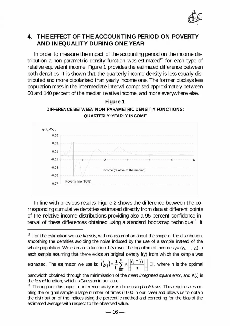
In order to measure the impact of the accounting period on the income distribution a non-parametric density function was estimated12 for each type of relative equivalent income. Figure 1 provides the estimated difference between both densities. It is shown that the quarterly income density is less equally distributed and more bipolarised than yearly income one. The former displays less population mass in the intermediate interval comprised approximately between 50 and 140 percent of the median relative income, and more everywhere else.

Figure 1 DIFFERENCE BETWEEN NON PARAMETRIC DENSITIY FUNCTIONS:

QUARTERLY-YEARLY INCOME

-0,07

-0,05

-0,03

-0,01

0,01

0,03

0,05

0 1 2 3 4 5 6

Income (relative to the median)

f(x) q -f(x) y

Poverty line (60%)

In line with previous results, Figure 2 shows the difference between the corresponding cumulative densities estimated directly from data at different points of the relative income distributions providing also a 95 percent confidence interval of these differences obtained using a standard bootstrap technique13. It

12 For the estimation we use kernels, with no assumption about the shape of the distribution, smoothing the densities avoiding the noise induced by the use of a sample instead of the whole population. We estimate a function f̂ (y)over the logarithm of incomes y=(y1, ..., yn) in each sample assuming that there exists an original density f(y) from which the sample was

n^ y − y 1 j iextracted. The estimator we use is: ( ) = ∑K ∀ j , where h is the optimal f y j h hi=1 bandwidth obtained through the minimisation of the mean integrated square error, and K(.) is the kernel function, which is Gaussian in our case. 13 Throughout this paper all inference analysis is done using bootstraps. This requires resampling the original sample a large number of times (1000 in our case) and allows us to obtain the distribution of the indices using the percentile method and correcting for the bias of the estimated average with respect to the observed value.

— 16 —


can be observed that when plotting this line of differences we find one single crossing of the x-axis which is very close to the value of median equivalent in-come. This implies that for every relative poverty line between 0 and that point, poverty incidence is larger using quarterly than using annual income. This difference is not large though, but it is still significantly different from zero at least up to 70 percent of the median, reaching its maximum between 50 and 60 percent (around an additional 1.2 percent of households are classified as poor using a quarterly income accounting period). This result has important consequences in terms of poverty rankings: it implies that within that interval the annual relative income distribution dominates the quarterly relative income distribution for the headcount ratio, i.e. the Foster, Green and Thorbecke index FGT(0)≡H14. It thus follows that all indices in the class of additively separable poverty measures satisfying the monotonicity axiom (including the rest of FGT family) will agree with the same ranking between distributions (Atkinson, 1987) for all poverty lines lying in that interval. This is precisely the interval which includes all the most usually chosen poverty thresholds.

Figure 2

DIFFERENCE BETWEEN CUMULATIVE DENSITIY FUNCTIONS: QUARTERLY-YEARLY INCOME

-2,0 -1,5 -1,0 -0,5 0,0 0,5 1,0 1,5 2,0

0 0,2 0,4 0,6 0,8 1 1,2 1,4 1,6 1,8 2 2,2 2,4 2,6 2,8 3

Income (relative to the median)

F(x)

q -F

(x)

y

Given our choice of poverty threshold (60 percent of the median) headcounts are larger using a quarterly income accounting period than using an annual one: 17.2 versus 16 percent of households (7.5 percent larger) are classified as poor. Even if we could consider this just a slight difference, there are three further relevant questions in order to evaluate all differences in the distributive analysis when deciding to use each of these alternative income concepts. The first one refers to the possibility that the use of different income ac

14 That is, there exists first-degree stochastic dominance for the censored distribution of annual relative income over the censored distribution of quarterly relative income.

— 17 —

1 1

1 1

1 1

1 1

1 1

1 1

1 1

counting periods may imply that poverty intensity and inequality differ more than what poverty incidence does. A second concern is related to the nature of re-rankings that may occur within the distribution when changing the income concept. Further, a third and very important question is that of whether or not both criteria identify the same households as poor i.e. to what extent do both concepts coincide in identifying the poor.

Regarding the first question, that concerned with the possibility that the use of different income accounting periods may imply that poverty intensity and inequality differ more than what poverty incidence does, we need to undertake a more detailed analysis of income distribution. Table 1 presents additional estimates for a group of poverty and inequality indices. Here we actually confirm that poverty indices accounting for poverty intensity and/or inequality within the poor provide larger divergences between the results obtained with each accounting period than the headcount ratio did constraining the analysis to poverty incidence. All divergences go in the same direction, as expected by the existence of head-count ratio dominance, indicating that the use of a quarterly accounting period results in higher poverty estimates. The poverty gap ratio is 22 percent higher, and the FGT family for α≥2 increasingly diverges with the poverty aversion parameter (i.e. the most sensitive the index to the extremely poor). In the case of Sen and Thon (or Sen modified) indices that do not belong to the additive separable class we also show that their results diverge in more than a 20 using different accounting periods.

Table 1

INCOME DISTRIBUTION ESTIMATES

Quarterly Annual (Q/A)*100 95% Confidence interval for the ratio (Q/A)*100

Poverty

Headcount ratio (%) (Index FGT(0)*100) Income gap ratio (%) Poverty gap ratio (%) (Index FGT(1)*100)

Index FGT(2) *100

Index FGT(3) *100

Index FGT(4) *100

Index FGT(5) *100

Sen index *100

Thon index *100

17.237 25.687

4.428

1.983

1.214

0.896

0.74

6.423

8.436

16.032 22.671

3.635

1.383

0.694

0.417

0.286

5.242

6.944

107.5 113.3

121.8

143.4

174.9

214.9

258.7

122.5

121.5

104.8 110.1

118.1

135.7

160.8

191.8

222.9

118.9

117.8

110.2 117.0

125.5

151.4

190.8

243.2

305.2

126.3

125.0

(Sigue)

— 18 —


(Continuación)

Quarterly Annual (Q/A)*100 95% Confidence interval for the ratio (Q/A)*100

Inequality

Theil (-1) Theil (0) Theil (1) Theil (2) Gini

944.7 0.208 0.169 0.225 0.311

176.8 0.153 0.147 0.180 0.295

534.3 136.6 114.9 124.8 105.3

296.4 129.6 111.1 115.1 104.4

1219.4 144.0 119.2 137.4 106.3

Also in Table 2 we present some inequality measures for the entire distribution. Indices show that, as it is theoretically expected (see Shorrocks, 1978), inequality increases as one uses shorter time measurement intervals. This divergence is found to be increasing with the level of inequality aversion (and thus the higher the sensitivity to the situation at the bottom of the distribution): the lower the parameter of inequality aversion the higher the divergence between short-time measurement intervals and longer time ones. This statistically significant result could have also been presumed by the existence of a single crossing observed between the respective distribution functions leading to seconddegree stochastic dominance (and consequently Lorenz Dominance). Figure 3 displays both Lorenz curves, showing that annual income curve is always above that of quarterly income. The difference is small but statistically significant.

Figure 3

LORENZ CURVES WITH QUARTERLY AND YEARLY INCOME

0

0,1

0,2

0,3

0,4

0,5

0,6

0,7

0,8

0,9

1

0 0,1 0,2 0,3 0,4 0,5 0,6 0,7 0,8 0,9 1 Income share

Pop

ulat

ion

shar

e

Quarterly Yearly

— 19 —

1 1 1 1 1 1 1 1 1

1 1 1 1 1 1 1 1

1 1 1 1 1 1 1 1

1 1 1 1 1 1 1 1

1 1 1 1 1 1 1 1

1 1 1 1 1 1 1 1

1 1 1 1 1 1 1 1

1 1 1 1 1 1 1 1

1 1 1 1 1 1 1 1

1 1 1 1 1 1 1 1

Additionally, evaluating the kind of re-rankings that occur to households when we move from quarterly income to annual income can help in evaluating the actual changes that take place in the income distribution when the income accounting period is changed. For this we construct a transition matrix on deciles defined by both income criteria (see Table 2). Between a third and four fifths of households are observed to remain in the same decile when changing the in-come criterion from quarterly to annual. Most changes in decile classification are observed within the deciles in the middle of the distribution while fewer changes take place around the tails. In general there are more movements affecting people with low income than affecting households in the upper tail of the income distribution. A fourth part of households in the first decile moves up, and the same happens to around thirty percent of those in the deciles two to six. Most changes are of a short range, i.e. they are moves to the neighbouring decile; given that only around 10 percent of households below the median with quarterly income move at least two deciles up when using annual income. Indeed, the proportion of households in the lowest deciles moving to the top of the distribution is insignificant. For instance, 25.5 percent of households in the first decile move up with yearly income, but only 2.2 percent effectively cross the median (the respective shares for the second decile are 29.3 and 3 percent). These results allow us to reject, in line with Ruggles (1990), the “college professors taking the summer off” scenario as being the typical case explaining differences between quarterly and yearly low-income groups.

Table 2 RE-RANKINGS IN THE DECILE DISTRIBUTION WITH DIFFERENT INCOME CRITERIA

Decile Yearly

Decile Quarterly 1 2 3 4 5 6 7 8 9 10

1 74.5 16.0 4.5 2.1 0.9 1.0 0.3 0.5 0.2 0.2

2 21.1 49.6 19.6 4.1 2.7 1.4 0.9 0.2 0.3 0.2

3 3.8 25.3 41.1 21.0 5.7 1.5 0.9 0.4 0.4 0.1

4 1.3 5.9 23.7 36.4 22.3 7.0 2.2 0.8 0.1 0.3

5 0.7 1.9 8.2 23.7 33.9 22.7 6.1 2.2 0.5 0.2

6 0.1 1.3 2.5 8.9 22.6 34.7 23.2 5.6 0.8 0.4

7 0.2 0.5 1.1 2.8 8.1 21.7 38.1 23.0 3.9 0.6

8 0.1 0.0 0.5 1.6 2.1 8.2 23.4 42.6 20.1 1.4

9 0.0 0.1 0.2 0.4 0.6 1.7 4.6 19.4 57.4 15.6

10 0.0 0.1 0.0 0.0 0.1 0.2 0.8 2.3 15.9 80.6

— 20 —

1 1 1 11 1 11 1 11 11 11 11 11 11 11. 1

11. 11. 1


Annual distribution

Decile Quarterly

Remain in the

same decile Moves upMoves up

Remain in the same decile or neighbor

Moves up (at least 2 deciles)

Moves down (at least 2 deciles)

1 2 3 4 5 6 7 8 9

10

74.5 49.6 41.1 36.4 33.9 34.7 38.1 42.6 57.4 80.6

25.5 29.3 29.9 32.6 31.7 29.9 27.5 21.6 15.6

0

0.0

21.1 29.1 31.0 34.5 35.4 34.4 35.8 27.0 19.4

90.5 90.3 87.3 82.4 80.3 80.5 82.8 86.1 92.3 96.6

9.5 9.7 8.9

10.3 9.0 6.8 4.5 1.4

0 0

0.0 0.0 3.8 7.3

10.8 12.8 12.7 12.5

7.7 3.5

Finally, regarding the third question, that concerning whether or not both criteria identify the same households as poor, Table 3 presents some results on the degree of coincidence in the classification of households as poor or nonpoor using each criterion. Of those identified as poor with annual income, one out of five is considered non-poor with quarterly income. The opposite is true for one out of four of the quarterly poor. At the same time, around 4 or 5 percent of those classified as non-poor with one criterion are not classified as such with the alternative one. In total, 7.4 percent of all households in the sample are classified differently when using both criteria. Clearly, the importance of this group of households depends on their distinct characteristics from the samples of poor and non-poor households.

Information contained in the same table provides us with some evidence on the stability of the poverty status all along the year previous to the household interview and on the importance of considering accounting periods shorter than a year in measuring household income. Focussing on quarterly income during the year previous to the interview we find that around 30 percent of all households in the sample are touched by poverty during at least one quarter of the year while only one out of three or these households are poor during the whole year long. That is, considering poverty within the year, the extent of poverty in the population increases significantly. Moreover, regarding the group of those considered non-poor on an annual basis, a significant amount of them (16 percent) were poor during at least one quarter of the year. As expected, the quarterly income criterion is more exigent in order to classify households as poor during a whole year given that only around a half of yearly poor households on an annual income accounting period basis were poor all along the year using a quarterly accounting period.

— 21 —

1 1

1 1

1 ,

1 1 11

1 1 1

1 1 1

1 11.

1 1

1 11 1

1 1 11

11

Table 3 HEADCOUNT RATIOS: ANNUAL AND QUARTERLY INCOME

All Annual non-poor Annual poor

Quarterly poor 17.24 5.15 80.56

Average of poor in each quarter

Poor during:

never (0 quarters)

1 quarter

2 quarters

3 quarters

at least 1 quarter

at least 2 quarters

at least 3 quarters

always (4 quarters)

18.15

70.62

8.44

6.95

5.68

29.38

20.94

13.99

8.31

5.73

84.1

9.78

5.21

0.91

15.9

6.12

0.91

0

83.23

0

1.43

16.06

30.66

100

98.56

82.5

51.84 All Quarterly non poor Quarterly poor

Annual Poor 16.03 3.77 74.93

Percentage of households classified differently with both criteria 7.4

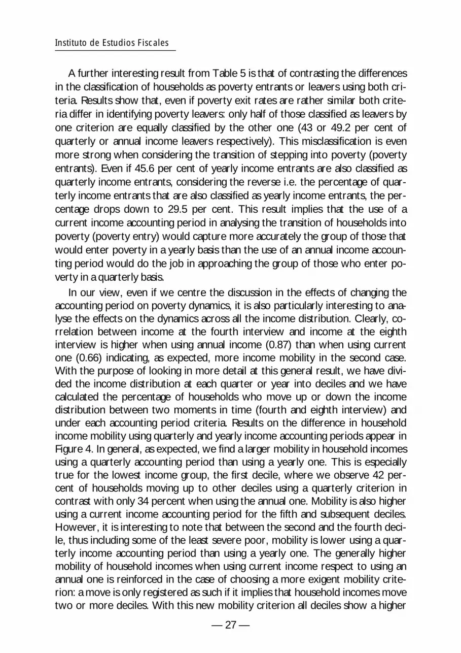
As we have just pointed out, the importance of analysing these issues is that of discovering if both criteria identify the same households types as poor or non-poor. Clearly, it could be the case that the situation in the demographic and socio-economic characteristics of the 7.4 percent of households who are classified differently under each criteria are remarkably similar to those of the poor or non-poor samples which would mean that the characterisation of poor households would basically coincide using anyone of these criteria. With the purpose of studying this we look at poverty incidence by population subgroups using each accounting period, measuring household characteristics at fourth interview. Table 4 presents headcount ratios for different typologies of households with each income definition and the ratio between them. The most outstanding feature is the strongly increasing divergence between both criteria when the household head's level of education increases. This implies a higher instability of incomes when the household head is highly educated than otherwise. The effect is especially clear from the point where a primary school level is completed. As a consequence, the more educated the household head is, the larger the differences in poverty rates between quarterly and annual income accounting periods. This is probably due to the fact that even if highly educated groups have a very low poverty risk, between 1.8 and 8.4 percent, they are subject to being identified as poor using a quarterly income accounting period

— 22 —


when, for example, they are sub-employed for a short period of time. However, given their large chances to get a better job, increasing their income accounting period rapidly decreases their poverty risk15. The fact that qualification is a relevant issue in explaining differences in the characteristics of households classified as poor under these two criteria is furtherly highlighted by the fact that household heads who are full-time qualified employees show the largest divergence in poverty rates (35 percent) according to labour market status. Other household characteristics which differ between samples are the fact of being headed by a 35 and 45 years old, headed by a female, being a household in a couple with one or two children, living in the largest townships or being a household whose head is self-employed or works part-time. All these characteristics register higher poverty rates measuring quarterly income during the fourth quarter than during the whole year. Finally, only a few number of characteristics show poverty rates based on an annual income concept which are slightly larger than poverty rates during the last quarter of the year. In our case this is most likely to happen in households with three or more children whose head is a non-qualified employee where the spouse is employed.

Table 4

HEAD-COUNT RATIO BY HOUSEHOLD TYPE

Quarterly Annual Q/A*100

Sex of household head

female head

male head

27.8

14.8

25.0

14.0

111.0

106.1

Education household head

illiterate

no studies

primary school

secondary (1st cycle)

secondary (2nd cycle)

university (3 years)


42.7

28.5

16.8

9.5

5.3

2.9

3.3

40.9

27.2

15.6

8.4

4.4

2.0

1.8

104.4

104.6

107.9

112.6

120.6

143.0

187.8

(Sigue)

15 The proportion of those holding a university degree ever touched by poverty is more than three times the poverty rate with yearly income: 7.1 (3 years degree) and 5.6 percent (5 years degree) compared to 2 and 1.8 percent respectively. Note here that in the Spanish context this becomes specially likely due to the high instability of young individuals holding an university degree in the labour market because of the existence of a large amount of qualified individuals with temporary contracts.

— 23 —

(Continuación)

Quarterly Annual Q/A*100

Household demographic type with children 15.2 14.3 106.2 lone or single parent 27.6 27.2 101.5 couple <=2 children 11.9 10.6 112.4 couple >=3 children 23.3 24.0 96.9 without children 19.1 17.6 108.5 Age group <35 13.1 12.3 106.3 35-45 13.2 11.8 111.6 45-55 13.1 12.0 109.2 55-65 18.1 17.5 103.2 ≥65 25.4 23.5 108.3 Size of municipality of residence <5,000 inhabitants 25.7 24.9 103.1 5,000-10,000 inhabitants 23.0 21.9 105.0 10,000-20,000 inhabitants 20.9 20.5 102.0 20,000-50,000 inhabitants 20.1 17.9 112.3 50,000-100,000 inhabitants 13.3 12.3 107.8 100,000-500,000 inhabitants 13.2 11.7 112.0 >500,000 inhabitants 11.4 10.1 113.0 Head labor market status full-time employed, qualified 3.7 2.7 135.0 full-time employed, non-qualified, agric 29.5 30.5 96.5 full-time employed, other non-qualified 16.4 17.8 92.3 full-time self-employed 14.8 13.0 113.9 Part-time (<13 h) employed 41.1 36.5 112.7 unemployed, with benefit 31.9 28.8 110.7 unemployed, without benefit 44.5 41.6 107.1 retired with pension 25.3 23.8 106.6 retired without pension 29.0 30.1 96.4 working at home 38.8 35.5 109.2 other situation 40.8 35.5 114.8 Spouse status no spouse 26.0 23.5 110.5 spouse employed 7.4 7.6 97.4 spouse not employed 16.7 15.6 107.2 All 17.2 16.0 107.5

— 24 —

5.


What differences do these results make compared to those already known in the literature? In this paper sub-annual incomes are measured each quarter rather than each month. As a consequence, we find that average quarterly poverty rate is around 14 percent higher than the annual rate16, while Ruggles and Williams (1986) found a larger difference measuring incomes every month: the average monthly poverty rate during a year was 25 percent higher than the annual rate (13.7 versus 11 percent). The difference could be perfectly explained by the smoothing effect imposed by a larger sub-annual period. Our results coincide with these two authors’ in that around a half of annual poor were poor all year long, and that the proportion of ever poor during a year is substantially higher than the proportion of annual poor (1.8 times in Spain, 2.4 in the US case). In both cases there is some difference across population subgroups: according to Ruggles and Williams the elderly and single parents were the demographic groups for whom poverty rates diverged the least, probably due to their dependency on social transfers. This result is replicated in the Spanish case, however a more detailed analysis in the present paper highlights the fact that qualification in employment is even more crucial to explain divergences across groups17 . In general in this paper we sustain that poverty and inequality are larger with quarterly income, the magnitude depending on the index but with generally larger effects the more sensitivity to the bottom of the distribution, something relevant to poverty analysis. This result contrasts with Böheim and Jenkins (2000)’s, who found more divergences in the upper tail, what they attributed mostly to measurement error.

5. THE SENSITIVITY OF INCOME DYNAMICS TO THE CHOICE OF ACCOUNTING PERIOD

So far we have concentrated the analysis on the effects of the accounting period on the income distribution during one year. The aim in this section is to open the discussion to the effects on income and poverty dynamics between two different years. For that purpose we restrict the previous sample to those households observed at least eight interviews (7,713 observations).

16 Note that our average quarterly poverty rate is higher than the rate computed at the fourth quarter. This is due to the fact that on average poverty rates decline during the interval used to construct the sample. 17 A comparison with Morris and Preston (1986) is more difficult due to the high variability in their results. Poverty rates using current income were 16 percent larger than annual income in 1968, 5 percent in 1977 but 34 percent lower in 1983. Differences between Gini coefficients were pretty small, 5 percent higher with annual incomes in the first year, similar in the second one and 6 percent lower in the third one. Our results were obtained using a pool of observations between 1985 and 1995, thus averaging divergences during that period.

— 25 —

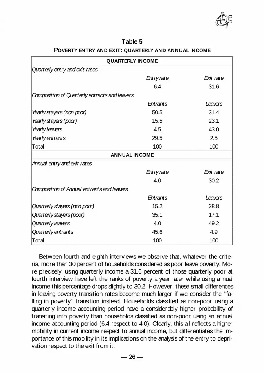
Table 5 POVERTY ENTRY AND EXIT: QUARTERLY AND ANNUAL INCOME

QUARTERLY INCOME

Quarterly entry and exit rates

Entry rate

6.4 Composition of Quarterly entrants and leavers

Entrants

Yearly stayers (non poor) 50.5 Yearly stayers (poor) 15.5 Yearly leavers 4.5 Yearly entrants 29.5 Total 100

Exit rate

31.6

Leavers

31.4 23.1 43.0 2.5 100

ANNUAL INCOME

Annual entry and exit rates

Entry rate

4.0 Composition of Annual entrants and leavers

Entrants

Quarterly stayers (non poor) 15.2 Quarterly stayers (poor) 35.1 Quarterly leavers 4.0 Quarterly entrants 45.6 Total 100

Exit rate

30.2

Leavers

28.8 17.1 49.2 4.9 100

Between fourth and eighth interviews we observe that, whatever the criteria, more than 30 percent of households considered as poor leave poverty. More precisely, using quarterly income a 31.6 percent of those quarterly poor at fourth interview have left the ranks of poverty a year later while using annual income this percentage drops slightly to 30.2. However, these small differences in leaving poverty transition rates become much larger if we consider the “falling in poverty” transition instead. Households classified as non-poor using a quarterly income accounting period have a considerably higher probability of transiting into poverty than households classified as non-poor using an annual income accounting period (6.4 respect to 4.0). Clearly, this all reflects a higher mobility in current income respect to annual income, but differentiates the importance of this mobility in its implications on the analysis of the entry to deprivation respect to the exit from it.

— 26 —


A further interesting result from Table 5 is that of contrasting the differences in the classification of households as poverty entrants or leavers using both criteria. Results show that, even if poverty exit rates are rather similar both criteria differ in identifying poverty leavers: only half of those classified as leavers by one criterion are equally classified by the other one (43 or 49.2 per cent of quarterly or annual income leavers respectively). This misclassification is even more strong when considering the transition of stepping into poverty (poverty entrants). Even if 45.6 per cent of yearly income entrants are also classified as quarterly income entrants, considering the reverse i.e. the percentage of quarterly income entrants that are also classified as yearly income entrants, the percentage drops down to 29.5 per cent. This result implies that the use of a current income accounting period in analysing the transition of households into poverty (poverty entry) would capture more accurately the group of those that would enter poverty in a yearly basis than the use of an annual income accounting period would do the job in approaching the group of those who enter poverty in a quarterly basis.

In our view, even if we centre the discussion in the effects of changing the accounting period on poverty dynamics, it is also particularly interesting to analyse the effects on the dynamics across all the income distribution. Clearly, correlation between income at the fourth interview and income at the eighth interview is higher when using annual income (0.87) than when using current one (0.66) indicating, as expected, more income mobility in the second case. With the purpose of looking in more detail at this general result, we have divided the income distribution at each quarter or year into deciles and we have calculated the percentage of households who move up or down the income distribution between two moments in time (fourth and eighth interview) and under each accounting period criteria. Results on the difference in household income mobility using quarterly and yearly income accounting periods appear in Figure 4. In general, as expected, we find a larger mobility in household incomes using a quarterly accounting period than using a yearly one. This is especially true for the lowest income group, the first decile, where we observe 42 percent of households moving up to other deciles using a quarterly criterion in contrast with only 34 percent when using the annual one. Mobility is also higher using a current income accounting period for the fifth and subsequent deciles. However, it is interesting to note that between the second and the fourth decile, thus including some of the least severe poor, mobility is lower using a quarterly income accounting period than using a yearly one. The generally higher mobility of household incomes when using current income respect to using an annual one is reinforced in the case of choosing a more exigent mobility criterion: a move is only registered as such if it implies that household incomes move two or more deciles. With this new mobility criterion all deciles show a higher

— 27 —

proportion of households moving up or down the income distribution using current income than using an annual one, with the only exception of the second decile where they coincide. This all implies that modifying the income accounting period may have different consequences for household income mobility depending on the point at which a household is situated within the income distribution at the initial moment. This is even more so if we use a simple mobility definition such as changing decile.

Figure 4

DIFFERENCES IN PERCENTAGES OF HOUSEHOLDS MOVING UP OR DOWN: QUARTERLY MINUS YEARLY INCOME

-4

-2

0

2

4

6

8

10

12

1 2 3 4 5 6 7 8 9 10

decile

%

At least one decile At least two deciles

In order to connect our results on poverty dynamics with those obtained in poverty statics, we are interested in analysing the differences in poverty transition rates (i.e. poverty exit and entry rates) for different demographic and socioeconomic groups of households when changing the income accounting period. Our interest is that of determining if those classified as poverty stayers or leavers under each criterion differ in their characteristics and therefore poverty dynamics analysis should consider some sensitivity analysis to the income accounting period chosen. Results on exit and entry rates by population subgroups appear in Table 6, which also provides the relationship between both (columns 3 and 6) in order to highlight for what characteristics quarterly and yearly rates diverge the most.

In Table 6 it can be observed that for most household characteristics one finds higher exit and entry poverty rates using a quarterly income accounting period than using an annual one. Some exceptions appear in poverty exit for households without children, with an employed spouse, whose head is between

— 28 —

1 1 1

1

1 1

1 1

1 1

1 1

1 1 1

1 1

1 1

1 1 1

1 1 1

1 1 1


55 and 65 years of age or is retired. However, a more interesting result here is that the magnitude of the discrepancy between annual and current income transition rates notably diverges across groups. There are characteristics which register differences that are higher than that of the mean household (first line of the columns), implying that households with the characteristic have a larger in-come mobility both into and out of the low income group than the mean household. This is the case of households headed by a young individual below 35 years of age. In contrast, households with a relatively large difference in the exit transition rate but a relatively low one in the entry rate are those whose income instability tends to promote households out of poverty in the short-run. These households are most likely to be households with children, living in large townships, whose head is unemployed or in other labour market status or whose spouse is not employed. Finally the characteristics which may imply a relatively high within the year mobility promoting a fall into poverty in the short-run are the employment of the head and the spouse and the fact of living in relatively small townships (below 50,000 inhabitants).

Table 6 ENTERING AND LEAVING POVERTY RATES BY HOUSEHOLD TYPE:

ANNUAL AND QUARTERLY INCOME

Exit rate Entry rate

Quarterly Annual Q/A*100 Quarterly Annual Q/A*100

ALL 31.58 30.2 104.6 6.36 4.04 157.4


female head 26.78 26.28 101.9 11.39 8.16 139.6

male head 33.79 31.89 106.0 5.40 3.23 167.2


illiterate, no studies, primary 30.67 29.62 103.5 8.15 4.98 163.7

secondary or university 38.13 35.54 107.3 2.87 2.21 129.9

Household demographic type

with children 39.40 34.26 115.0 6.08 3.73 163.0

without children 26.43 27.54 96.0 6.67 4.31 154.8

Age group

<35 38.79 28.77 134.8 8.89 5.08 175.0

35-45 39.45 33.92 116.3 4.63 2.78 166.5

45-55 38.84 39.73 97.8 5.11 3.20 159.7

55-65 32.07 33.48 95.8 5.92 4.52 131.0

≥65 23.35 23.96 97.5 7.74 4.80 161.3

(Sigue)

— 29 —

1 1 1

1 1

1 1 1

1 1

1 1

1 1 1

1 1

(Continuación)

Exit rate Entry rate

Quarterly Annual Q/A*100 Quarterly Annual Q/A*100

Size of municipality of residence

<50,000 inh. 27.73 28.90 96.0 8.75 5.03 174.0

≥50,000 inh.

Head labour market status

36.96 32.10 115.1 4.57 3.29 138.9

employed 38.62 39.39 98.0 5.07 2.80 181.1

unemployed 40.53 27.07 149.7 16.53 12.61 131.1

retired 25.57 26.43 96.7 7.70 5.33 144.5

other

Spouse status

30.31 20.66 146.7 12.76 10.61 120.3

no spouse 26.14 26.22 99.7 10.80 7.58 142.5

spouse employed 39.17 42.17 92.9 4.01 1.31 306.1

spouse not employed 34.24 30.94 110.7 5.62 3.66 153.6

The literature has also provided some evidence on the effect of the accounting period on income dynamics. Our results confirm, once again, Ruggles (1990)’s view on the fact that quarterly income mobility is not strongly affected by people with high annual income. In our case we find a quite similar result to hers: 92 percent of quarterly entrants in poverty have an annual income that is below the corresponding median. If we compare our results with those presented by Böheim and Jenkins (2000) using the BHPS a first point of divergence is that the difference we find in the correlation between the incomes of one year and the next using both accounting periods is sensibly larger than that found by these authors18. However, our results coincide with theirs in detecting only a slight difference between the percentage of households remaining in the same decile during two years using a current income criterion (45.7 per cent) and using an annual income one (43 per cent). In any case, we furtherly obtain that there are important differences in mobility depending on the initial position of household income in the distribution. Further, an important distinction between our findings and those obtained by these authors refers to the fact that in the British panel results there is not much difference between exit and entry

18 In their case they face a high variability of this difference through time. They find particularly small differences between some waves of the panel (in some cases they even obtain a reverse sign of the correlation coefficient). The largest difference they found was that of a correlation of 0.81 for current income and a correlation of 0.64 for annual income. In any case, their estimates of the difference are more stable when removing some small percentage of the highest incomes.

— 30 —


rates into the low-income group using a different income accounting period. In contrast, our estimates reflect a much more substantial difference in the estimation of poverty entry rates.

6. CONCLUSIONS

In this paper we have offered additional evidence on the effect of the accounting period on the income distribution, mainly on the analysis of poverty incidence, transitions into and out of poverty and the composition of the poor. We undertake the analysis of the sensitivity of income distribution estimates using a longitudinal survey which is similar to the SIPP: the Spanish Encuesta Continua de Presupuestos Familiares (ECPF) and using a fine weighting method that takes both representativity and attrition in the panel into account. Using this data source we are able to use sub-annual periods of income and to reconstruct the household's complete picture of incomes over the year. More precisely, in our static approach we compare the annual income of households observed four times in the survey (the sum of their first four quarterly incomes) with their quarterly income obtained between their third and their fourth interview in the survey. In the dynamic approach, instead, we analyse the income change experienced by a household observed during two years in the panel. Here we must contrast the level of income mobility obtained if comparing household quarterly income at fourth and eighth quarters with the level of in-come mobility obtained if comparing the first year's annual income (the sum of their first four quarterly incomes) and the second year's annual income (the sum of their last four quarterly incomes).

Results indicate that there are some relevant differences in poverty statics and dynamics when we use different income accounting periods. Most precisely, even if differences in poverty incidence are small, a quarterly income accounting period registers statistically significant higher poverty levels under a large battery of poverty indices. The magnitude of the difference is larger the more sensible the index to the situation at the bottom of the distribution. Also, some interesting differences are found in terms of the composition of the group of the poor: using quarterly income we find more highly qualified poor households. Other household characteristics which differ between samples are the fact of being headed by a 35 and 45 years old female or being a couple with one or two children living in the largest townships whose head is self-employed or works part-time.

As expected, we find a higher mobility in using a quarterly than using an annual accounting period. In any case it is most interesting to note that there are some relevant differences depending on the direction of the movement (diffe

— 31 —

rences are larger in poverty entry than in poverty exit) and the point of the in-come distribution where they happen (the largest difference appears in the first decile). Similarly to the case in poverty statics, the identification of households moving into and out of the poor group differ with the accounting period. Most groups show higher entry and poverty rates using current income than using annual income, with the largest difference affecting households headed by young individuals (below 35 years of age). This implies that their income mobility within the year is high. In contrast, households with children, living in large townships, whose head is unemployed or in other labour market status or whose spouse is not employed are most likely to be households with a positive household income instability within the year, that is, household income instability often implies a higher poverty exit. Finally the characteristics which may imply a relatively high within the year mobility promoting a fall into poverty in the short-run are the employment of the head and the spouse and the fact of living in relatively small townships (below 50,000 inhabitants).

In sum, in this paper we sustain that income instability is larger using a current income accounting period than using an annual one, and that this has important consequences for the measurement of poverty levels during a year, for the identification of who has low income and for determining how many households (and with what characteristics) fall into poverty between two given years. Thus, the analysis of the sensitivity of results on poverty statics and dynamics to the accounting period chosen seems rather important in several cases. Moreover, in our view, these results are important in order to guide social policies aimed at the short-run poor, as it is the case for many minimum income guaranteed schemes and emergency aids designed by modern societies based on sub-annual means tested benefits.

— 32 —


APPENDIX A

Accounting for different selection and attrition probabilities

In this study we use a sample of Spanish households interviewed quarterly between 1985 and 1995. In a first stage, we construct quarterly and annual in-come relative to the contemporary median as described in the text. In a second stage, we construct a pool of all households with at least four surveys completed containing information about each interview in which they participate. This pool is then used to conduct the analysis of income distribution in a year (between first and fourth interview). These samples used in both stages suffer from a double problem of lack of representativeness: different sampling selection of households due to sample design and non-response, and different attrition probabilities by household characteristics of achieving the fourth interview. As Rose (2000) suggests, in order to preserve representativeness in our final sample we need to compute the appropriate weights such that we are able to control for both potential biases.

In generating weights correcting for both biases we interpret in a simplified way the pool as the result of two sampling procedures. First, at a given quarter t households in the population (of size Nt) are randomly selected assigning different a priori probabilities, leading to what we call Sample 1 at t with size nt. Then in order to take attrition into account, a resampling process is undertaken attaching again different new a priori probabilities to households present in Sample 1, such that the sample size is reduced to mt<nt obtaining Sample 2. In order to preserve representativeness in this sample, we compute the a priori probability for each household of being in that sample and then obtain its actual weight, which will be inversely proportional to that probability.

Let us define Sj to be a random variable that equals 1 if a given household is selected in Sample j (j=1, 2) and 0 otherwise. Then the probability of household i (i=1,..., mt) of being in Sample 2 at quarter t is given by:

Pit (S2 = 1) = Pit (S2 = 1/S1 = 1)Pit (S1 = 1) , i=1,..., m; t=1,..., T,

where probability of being selected in the first sample, Pit(S1=1), is known be-cause it is usual to interpret cross-sectional weights provided by Statistical Offices as being proportional to the inverse of the selection probability. Pit(S2=1/S1=1) is the probability of being selected in Sample 2 conditioned to having been selected in Sample 1. It is estimated using a probit regression on a set of relevant characteristics over a pool of the sample for the entire period as explained in Section 3. Thus, the weight attached to the ith household in Sample 2 at quarter t is defined as being proportional to the inverse of the estimated

— 33 —

probability of being selected in that sample, re-scaled using a scaling factor k to sum up the final size (mt):

m

wit = k , ∑

t

wit = mt .^ i=1P (S = 1)it 2

In Sample 2 for each quarter we compute quarterly and annual equivalent in-come relative to the contemporary median using these weights. In the second stage we construct a pool of observations with all households that reached, at least, a fourth interview (the size of the pool is M4). Weights at the fourth interview are re-scaled (using the scale factor α) so that they sum up the size of the pool:

M4 4 4wi = αwis , where s = t such that i is in its 4th interview; ∑wi = M4 .

i=1

For the longitudinal analysis we proceed in a very similar way. The difference is that in this case the pool is constructed with all households observed all 8 interviews, constructing new weights w8

i in a similar way as w4 i.

The results from the previous procedure appear in Table A1. The most outstanding feature is that final weights need to correct for misrepresentation of households living both in the country's largest cities (more than 500,000 inhabitants) and in middle-sized ones (20,000-50,000 inhabitants). That is the result of both, a low probability of being selected and a high attrition rate. This is also the case for households whose heads are highly educated, female, with no spouse, below 35 year of age or are unemployed with benefit. We can observe that the correlation between sampling and attrition weights is 13 percent in the first pool and 15 percent in the second one. Further, the correlation between these two types of weights and the final ones is 94 and 83 respectively in the first case, and 41 and 61 respectively in the second one. This suggests that the sampling procedure explains most of the variability in these weights, though attrition becomes more important as we move from a minimum of four interviews to a minimum of eight.

— 34 —


Table A1

WEIGHTS CONTROLLING FOR SAMPLING SELECTION AND/OR

ATTRITION BY CHARACTERISTICS

Ratio between the average weights of households with a given characteristic to the mean

Pool 1 (at least 4 interviews)


Only Selection

Only Attrition

Both w4

Only Selection

Only Attrition

Both w8


female head 1.02 1.07 1.09 1.02 1.12 1.15

male head 1.00 0.99 0.98 1.00 0.98 0.97


illiterate 0.99 0.99 0.99 1.05 0.97 1.01

no studies 1.01 0.95 0.96 1.02 0.95 0.96

primary school





0.98

1.01

1.03

1.02

1.06

0.98

1.05

1.08

1.11

1.18

0.96

1.05

1.10

1.13

1.24

0.97

1.03

1.02

1.00

1.03

0.95

1.07

1.12

1.22

1.35

0.93

1.08

1.15

1.21

1.42


with children 0.99 0.98 0.98 0.99 1.00 0.99

lone or single parent

couple <=2 children

couple >=3 children

without children

0.99

1.00

0.97

1.01

1.05

0.98

0.95

1.02

1.04

0.98

0.93

1.02

1.02

0.99

1.00

1.00

1.16

0.99

0.99

1.00

1.19

0.98

0.98

1.01

Age group

<35 1.02 1.06 1.08 1.02 1.14 1.16

35-45 1.00 1.00 1.00 1.00 1.03 1.03

45-55 1.00 0.97 0.97 0.99 0.96 0.95

55-65 0.99 0.97 0.97 0.99 0.94 0.94

≥65 0.99 1.02 1.01 1.00 1.00 0.99

(Sigue)

— 35 —

(Continuación)



Only Selection

Only Attrition

Both w4

Only Selection

Only Attrition

Both w8


<5,000 inh. 0.95 0.90 0.85 0.94 0.80 0.75

5,000-10,000 inh. 1.00 0.91 0.91 1.02 0.87 0.88

10,000-20,000 inh. 0.93 0.95 0.88 0.93 0.90 0.83

20,000-50,000 inh. 1.05 1.03 1.07 1.04 1.05 1.09

50,000-100,000 inh. 0.86 1.08 0.91 0.91 1.14 1.01

100,000-500,000 inh. 0.92 1.02 0.93 0.92 1.05 0.96

>500,000 inh. 1.33 1.12 1.48 1.33 1.26 1.65

Head labor market status

f-t employed, qualified 1.01 1.02 1.04 1.01 1.05 1.06

f-t employed, non-qual, agric 1.02 0.89 0.91 1.04 0.82 0.86

f-t employed, other non-qual 1.00 0.97 0.98 1.05 0.98 1.02

f-t self-employed 0.97 0.95 0.93 0.96 0.91 0.88

<13 h. employed 0.98 0.99 1.00 0.98 1.03 1.01

unemployed, with benefit 1.13 1.02 1.15 1.03 0.97 1.02

unemployed, without benefit 1.05 0.97 1.02 1.04 1.02 1.04

retired with pension 0.99 1.01 0.99 0.99 0.99 0.98

retired without pension 1.00 1.03 1.00 0.99 0.98 0.97

working at home 1.02 1.04 1.10 1.00 1.27 1.29

other situation 1.00 1.24 1.23 0.98 1.32 1.27

Spouse status

no spouse 1.02 1.08 1.10 1.03 1.12 1.16

spouse employed 1.03 1.00 1.03 1.02 1.01 1.02

spouse not employed 0.99 0.97 0.96 0.99 0.96 0.94

— 36 —

1 1 1

1 1

1

1

1 1 1

1 1 1

1 1


APPENDIX B TABLES

Table B1

DESCRIPTIVE STATISTICS OF THE SAMPLE USED IN THE STATIC ANALYSIS

(18,008 observations)

Population share

Quarterly income*100

Annual income*100

Quarterly/Annual income*100


female head

male head

18.7

81.3

103.5

121.2

102.9

119.1

100.6

101.7


illiterate 4.0 75.2 75.1 100.2

no studies 22.2 89.4 88.3 101.2

primary school 44.0 108.4 106.5 101.8

secondary (1st cycle) 10.6 124.1 122.0 101.7

secondary (2nd cycle) 10.1 151.2 148.0 102.1

university (3 years) 4.6 186.9 184.5 101.3

university (5 years) 4.4 230.0 228.7 100.6


with children 47.3 115.7 114.0 101.5

lone or single parent 3.7 96.6 94.1 102.7

couple <=2 children 35.2 122.1 120.5 101.3

couple >=3 children 8.4 97.0 95.2 101.9

without children 52.7 119.8 118.0 101.6

Age group

<35 14.9 127.8 125.3 101.9

>=35-<45 19.4 122.9 121.5 101.2

>=45-<55 19.7 126.3 123.4 102.4

>=55-<65 20.8 122.9 120.5 102.0

>=65 25.2 97.2 97.0 100.2

(Sigue)

— 37 —

1 1

1 1 1

1

1 1 1

1 1

1 1 1

1 1

1 1 1 1

1 1

1

1 1 1

1 1 1 1

(Continuación)

Population share


Annual income*100



<5,000 inh. 16.3 97.9 95.6 102.3

5,000-10,000 inh. 9.1 99.5 98.4 101.1

10,000-20,000 inh. 9.3 103.4 102.5 100.9

20,000-50,000 inh. 11.2 107.9 105.8 102.0

50,000-100,000 inh. 10.6 120.4 117.4 102.6

100,000-500,000 inh. 21.9 127.2 125.8 101.1

>500,000 inh. 21.6 141.5 139.8 101.2


f-t employed, qualified 34.2 148.5 146.1 101.6

f-t employed, non-qual, agric 1.7 88.8 83.1 106.8

f-t employed, other non-qual 8.2 102.2 99.6 102.6

f-t self-employed 13.1 122.0 119.3 102.3

<13 h. employed 1.2 80.1 79.3 101.0

unemployed, with benefit 0.2 102.2 113.7 90.0

unemployed, without benefit 4.6 80.1 80.5 99.6

retired with pension 33.6 98.4 97.7 100.8

retired without pension 1.5 111.6 105.6 105.7

working at home 0.8 93.5 91.6 102.0

other situation 0.8 92.2 96.3 95.8

Spouse status

no spouse 22.7 106.4 105.1 101.2

spouse employed 17.0 158.5 154.8 102.4

spouse not employed 60.3 110.8 109.3 101.3

Note: Incomes are the mean value of the income of the corresponding group respect to the contemporary quarter's income median using either an annual or a quarterly income accounting period.

— 38 —


Table B2

DESCRIPTIVE STATISTICS OF THE SAMPLE USED IN THE DYNAMIC ANALYSIS

(7,713 observations)

Population share


Annual income*100



female head 18.7 100.88 100.66 100.2

male head 81.3 118.54 117.40 101.0


illiterate 14.3 173.73 174.90 198.4

no studies 22.0 189.38 187.83 101.8

primary school





43.5

10.8

10.3

14.6

14.5

107.46

116.14

144.65

185.24

214.93

105.77

116.99

144.91

182.89

216.01

101.6

199.3

199.8

101.3

199.5


with children 47.0 112.31 111.76 100.5

lone or single parent

couple <=2 children

couple >=3 children

without children

14.0

34.9

18.1

53.0

196.51

117.41

198.18

117.84

193.84

117.66

195.20

116.50

102.8

199.8

103.1

101.1

Age group

<35 14.7 121.07 120.67 100.3

>=35-<45 19.4 118.23 118.19 100.0

>=45-<55 19.5 124.63 121.79 102.3

>=55-<65 21.0 123.33 120.88 102.0

>=65 25.4 195.66 196.33 199.3

(Sigue)

— 39 —

1 1

1 1 1

1 1

1

1 1 1

1 1 1

1 1 1 1

1 1 1 1

1 1 1 1

1 1

1 1 1 1

1 1 1 1

1 1

(Continuación)

Population share


Annual income*100



<5,000 inh. 16.0 96.56 93.48 103.3

5,000-10,000 inh. 9.1 98.35 97.95 100.4

10,000-20,000 inh. 9.3 102.83 103.62 99.2

20,000-50,000 inh. 11.1 105.51 106.07 99.5

50,000-100,000 inh. 10.9 119.04 115.75 102.8

100,000-500,000 inh. 21.9 123.28 122.99 100.2

>500,000 inh. 21.6 136.43 135.74 100.5


f-t employed, qualified 35.0 141.84 140.66 100.8

f-t employed, non-qual, agric 1.6 89.29 83.37 107.1

f-t employed, other non-qual 8.1 96.09 94.12 102.1

f-t self-employed 57.4 122.59 119.87 102.3

<13 h. employed 1.0 78.14 79.65 98.1

unemployed, with benefit 0.2 82.54 88.71 93.0

unemployed, without benefit 4.5 77.03 80.37 95.8

retired with pension 33.6 99.02 98.28 100.8

retired without pension 1.8 90.60 92.61 97.8

working at home 0.7 88.00 88.10 99.9

other situation 0.9 111.39 120.67 92.3

Spouse status

no spouse 23.1 104.97 104.43 100.5

spouse employed 17.0 150.02 146.33 102.5

spouse not employed 59.9 109.36 109.00 100.3

Note: Incomes are the mean value of the income of the corresponding group respect to the contemporary quarter's income median using either an annual or a quarterly income accounting period.

— 40 —

REFERENCES

ATKINSON, A. (1987): “On the measurement of poverty”, Econometrica, 55, pp. 244-263.

BÖHEIM, R. and JENKINS, S. (2000): “Do current income and annual income measures provide different pictures of Britain’s income distribution?”, Working Paper 2000-16, Institute for Social and Economic Research, University OF ESSEX.

BUHMANN, B., RAINWATER, L., SCHMAUS, G. and SMEEDING, T. (1988): “Equivalence scales, Well-Being, Inequality and Poverty: Sensitive Estimates across ten countries using the Luxembourg Income Study (LIS) database”, Review of Income and Wealth, 34, pp. 115-142.

BRADBURY, B., JENKINS, S. P. and MICKLEWRIGHT, J. (2001): “Conceptual and measurement issues”, in B. Bradbury, S. P. Jenkins and J. Micklewright (ed.) The dynamics of child poverty in industrialised countries, pp. 27-61, Cambridge University Press, Unicef.

BUCK, N., ERMISCH, J. F., JENKINS, S. P. (1995): “Choosing a longitudinal survey design: the issues”, Occasional Paper 96-1, Institute for Social and Economic Research, University of Essex.

BUHMANN, B., RAINWATER, L., SCHMAUS, G. and SMEEDING, T. (1988): “Equivalence scales, Well-Being, Inequality and Poverty: Sensitive Estimates across ten countries using the Luxembourg Income Study (LIS) database”, Review of Income and Wealth, 34, pp. 115-142.

CANTÓ, O. (1998): The Dynamics of Poverty in Spain: The Permanent and Transitory Poor, unpublished Ph.D. dissertation, European University Institute, Florence.

COULTER, F., COWELL, F. and JENKINS, S. (1992a): “Differences in needs and assessment of income distributions”, Bulletin of Economic Research, 44, pp. 77-124.

– (1992b): “Equivalence scale relativities and the extent of inequality and poverty”, Economic Journal, 102, pp. 1067-1082.

DHSS (1988): Low Income Statistics: Report and Technical Review, London: Department of Health and Social Security.

DUCLOS, J. Y. and MERCADER PRATS, M. (1999): “Household Needs and Poverty: With Application to Spain and the UK”, Review of Income and Wealth, 45 (1), pp. 77-98.

GOTTSCHALK (1997): Inequality, Income Growth, and Mobility: The Basic Facts, Journal of Economic Perspectives; 11(2), Spring 1997, pp. 21-40.

— 41 —

JENKINS, S.P. (1999): “Modelling household income dynamics”, ESRC Research Centre on Micro-Social Change, Working Paper 99-1, ISER - Institute for Social and Economic Research, University of Essex, Colchester.

JENKINS, S. P. and LAMBERT, P. (1997): “Three ‘I’s of poverty curves, with an analysis of UK poverty trends”, Oxford Economic Papers, 49, pp. 317-327.

– (1998a): “Three ‘I’s of poverty curves and poverty dominance: TIPs for poverty analysis”, Research on Economic Inequality, vol. 8.

– (1998b): “Ranking poverty gap distributions: further TIPs for poverty analysis”, Research on Economic Inequality, vol. 8.

KALTON, G. and BRICK, M. (2000): “Weighting in household panel surveys” in D. Rose (ed), Researching social and economic change. The uses of household panel studies, pp. 96-112, London: Routledge.

LUTTMER, E. F. P. (2001): “Measuring Poverty Dynamics and Inequality in Transition Economies: Disentangling Real Events from Noisy Data”, Unpublished manuscript, University of Chicago.

MORRIS, N. and PRESTON, I. (1986): “Inequality, poverty and the redistribution of income”, Bulletin of Economic Research, 38, pp. 277-344.

NOLAN, B. (1987): Income Distribution and the Macroeconomy, Cambridge University Press, Cambridge.

RUGGLES, P. (1990): Drawing the line: alternative poverty measures and their implications for public policy, The Urban Institute Press, Washington.

RUGGLES, P. and WILLIAMS, R. (1986): “Transitions in and out of poverty: new data from the Survey of Income Participation”, Urban Institute Research Paper, December, The Urban Institute, Washington.

– (1989): “Longitudinal measures of poverty: accounting for income and assets over time”, Review of Income and Wealth, 35 (3), pp. 225-244.

SHORROCKS, A.F. (1978): “Income inequality and income mobility”, Journal of Economic Theory, 19: pp. 376-93.

WALKER, R. (1994): Poverty Dynamics: Issues and Examples, Avebury, Aldershot. WINKELS, J. W. and DAVIES, S. (2000): “Panel attrition”, in D. Rose (ed), Resear

ching social and economic change. The uses of household panel studies, pp. 7995, Routledge, London.

— 42 —

NORMAS DE PUBLICACIÓN DE PAPELES DE TRABAJO DEL INSTITUTO DE ESTUDIOS FISCALES

Esta colección de Papeles de Trabajo tiene como objetivo ofrecer un vehículo de expresión a todas aquellas personas interasadas en los temas de Economía Pública. Las normas para la presentación y selección de originales son las siguientes:

1. Todos los originales que se presenten estarán sometidos a evaluación y podrán ser directamente aceptados para su publicación, aceptados sujetos a revisión, o rechazados.

2. Los trabajos deberán enviarse por duplicado a la Subdirección de Estudios Tributarios. Instituto de Estudios Fiscales. Avda. Cardenal Herrera Oria, 378. 28035 Madrid.

3. La extensión máxima de texto escrito, incluidos apéndices y referencias bibliográfícas será de 7000 palabras.

4. Los originales deberán presentarse mecanografiados a doble espacio. En la primera página deberá aparecer el título del trabajo, el nombre del autor(es) y la institución a la que pertenece, así como su dirección postal y electrónica. Además, en la primera página aparecerá también un abstract de no más de 125 palabras, los códigos JEL y las palabras clave.

5. Los epígrafes irán numerados secuencialmente siguiendo la numeración arábiga. Las notas al texto irán numeradas correlativamente y aparecerán al pie de la correspondiente página. Las fórmulas matemáticas se numerarán secuencialmente ajustadas al margen derecho de las mismas. La bibliografía aparecerá al final del trabajo, bajo la inscripción “Referencias” por orden alfabético de autores y, en cada una, ajustándose al siguiente orden: autor(es), año de publicación (distinguiendo a, b, c si hay varias correspondientes al mismo autor(es) y año), título del artículo o libro, título de la revista en cursiva, número de la revista y páginas.

6. En caso de que aparezcan tablas y gráficos, éstos podrán incorporarse directamente al texto o, alternativamente, presentarse todos juntos y debidamente numerados al final del trabajo, antes de la bibliografía.

7. En cualquier caso, se deberá adjuntar un disquete con el trabajo en formato word. Siempre que el documento presente tablas y/o gráficos, éstos deberán aparecer en ficheros independientes. Asimismo, en caso de que los gráficos procedan de tablas creadas en excel, estas deberán incorporarse en el disquete debidamente identificadas.

Junto al original del Papel de Trabajo se entregará también un resumen de un máximo de dos folios que contenga las principales implicaciones de política económica que se deriven de la investigación realizada.

— 43 —

PUBLISHING GUIDELINES OF WORKING PAPERS AT THE INSTITUTE FOR FISCAL STUDIES

This serie of Papeles de Trabajo (working papers) aims to provide those having an interest in Public Economics with a vehicle to publicize their ideas. The rules governing submission and selection of papers are the following:

1. The manuscripts submitted will all be assessed and may be directly accepted for publication, accepted with subjections for revision or rejected.

2. The papers shall be sent in duplicate to Subdirección General de Estudios Tributarios (The Deputy Direction of Tax Studies), Instituto de Estudios Fiscales (Institute for Fiscal Studies), Avenida del Cardenal Herrera Oria, nº 378, Madrid 28035.

3. The maximum length of the text including appendices and bibliography will be no more than 7000 words.

4. The originals should be double spaced. The first page of the manuscript should contain the following information: (1) the title; (2) the name and the institutional affiliation of the author(s); (3) an abstract of no more than 125 words; (4) JEL codes and keywords; (5) the postal and e-mail address of the corresponding author.

5. Sections will be numbered in sequence with arabic numerals. Footnotes will be numbered correlatively and will appear at the foot of the corresponding page. Mathematical formulae will be numbered on the right margin of the page in sequence. Bibliographical references will appear at the end of the paper under the heading “References” in alphabetical order of authors. Each reference will have to include in this order the following terms of references: author(s), publishing date (with an a, b or c in case there are several references to the same author(s) and year), title of the article or book, name of the journal in italics, number of the issue and pages.

6. If tables and graphs are necessary, they may be included directly in the text or alternatively presented altogether and duly numbered at the end of the paper, before the bibliography.

7. In any case, a floppy disk will be enclosed in Word format. Whenever the document provides tables and/or graphs, they must be contained in separate files. Furthermore, if graphs are drawn from tables within the Excell package, these must be included in the floppy disk and duly identified.

Together with the original copy of the working paper a brief two-page summary highlighting the main policy implications derived from the research is also requested.

— 45 —

1

1

1

1

1

1

1

1

1

ÚLTIMOS PAPELES DE TRABAJO EDITADOS POR EL

INSTITUTO DE ESTUDIOS FISCALES

2000

1/00 Crédito fiscal a la inversión en el impuesto de sociedades y neutralidad impositiva: Más evidencia para un viejo debate. Autor: Desiderio Romero Jordán. Páginas: 40.

2/00 Estudio del consumo familiar de bienes y servicios públicos a partir de la encuesta de presupuestos familiares. Autores: Ernesto Carrilllo y Manuel Tamayo. Páginas: 40.

3/00 Evidencia empírica de la convergencia real. Autores: Lorenzo Escot y Miguel Ángel Galindo. Páginas: 58.

Nueva Época

4/00 The effects of human capital depreciation on experience-earnings profiles: Evidence salaried spanish men. Autores: M. Arrazola, J. de Hevia, M. Risueño y J. F. Sanz. Páginas: 24.

5/00 Las ayudas fiscales a la adquisición de inmuebles residenciales en la nueva Ley del IRPF: Un análisis comparado a través del concepto de coste de uso. Autor: José Félix Sanz Sanz. Páginas: 44.

6/00 Las medidas fiscales de estímulo del ahorro contenidas en el Real Decreto-Ley 3/2000: análisis de sus efectos a través del tipo marginal efectivo. Autores: José Manuel González Páramo y Nuria Badenes Plá. Páginas: 28.

7/00 Análisis de las ganancias de bienestar asociadas a los efectos de la Reforma del IRPF sobre la oferta laboral de la familia española. Autores: Juan Prieto Rodríguez y Santiago Álvarez García. Páginas 32.

8/00 Un marco para la discusión de los efectos de la política impositiva sobre los precios y el stock de vivienda. Autor: Miguel Ángel López García. Páginas 36.

9/00 Descomposición de los efectos redistributivos de la Reforma del IRPF. Autores: Jorge Onrubia Fernández y María del Carmen Rodado Ruiz. Páginas 24.

10/00 Aspectos teóricos de la convergencia real, integración y política fiscal. Autores: Lorenzo Escot y Miguel Ángel Galindo. Páginas 28.

— 47 —

1

1

1

1

1

1

1

1

1

2001

1/01 Notas sobre desagregación temporal de series económicas. Autor: Enrique M. Quilis. Páginas 38.

2/01 Estimación y comparación de tasas de rendimiento de la educación en España. Autores: M. Arrazola, J. de Hevia, M. Risueño y J. F. Sanz. Páginas 28.

3/01 Doble imposición, “efecto clientela” y aversión al riesgo. Autores: Antonio Bustos Gisbert y Francisco Pedraja Chaparro. Páginas 34.

4/01 Non-Institutional Federalism in Spain. Autor: Joan Rosselló Villalonga. Páginas 32.

5/01 Estimating utilisation of Health care: A groupe data regression approach. Autora: Mabel Amaya Amaya. Páginas 30.

6/01 Shapley inequality descomposition by factor components. Autores: Mercedes Sastre y Alain Trannoy. Páginas 40.

7/01 An empirical analysis of the demand for physician services across the European Union. Autores: Sergi Jiménez Martín, José M. Labeaga y Maite Martínez-Granado. Páginas 40.

8/01 Demand, childbirth and the costs of babies: evidence from spanish panel data. Autores: José M.ª Labeaga, Ian Preston y Juan A. Sanchis-Llopis. Páginas 56.

9/01 Imposición marginal efectiva sobre el factor trabajo: Breve nota metodológica y comparación internacional. Autores: Desiderio Romero Jordán y José Félix Sanz Sanz. Páginas 40.

10/01 A non-parametric decomposition of redistribution into vertical and horizontal components. Autores: Irene Perrote, Juan Gabriel Rodríguez y Rafael Salas. Páginas 28.

11/01 Efectos sobre la renta disponible y el bienestar de la deducción por rentas ganadas en el IRPF. Autora: Nuria Badenes Plá. Páginas 28.

12/01 Seguros sanitarios y gasto público en España. Un modelo de microsimulación para las políticas de gastos fiscales en sanidad. Autor: Ángel López Nicolás. Páginas 40.

13/01 A complete parametrical class of redistribution and progressivity measures. Autores: Isabel Rabadán y Rafael Salas. Páginas 20.

14/01 La medición de la desigualdad económica. Autor: Rafael Salas. Páginas 40.

— 48 —

15/01 Crecimiento económico y dinámica de distribución de la renta en las regiones de la UE: un análisis no paramétrico. Autores: Julián Ramajo Hernández y María del Mar Salinas Jiménez. Páginas 32.

16/01 La descentralización territorial de las prestaciones asistenciales: efectos sobre la igualdad. Autores: Luis Ayala Cañón, Rosa Martínez López y Jesus Ruiz-Huerta. Páginas 48.

17/01 Redistribution and labour supply. Autores: Jorge Onrubia, Rafael Salas y José Félix Sanz. Páginas 24.

18/01 Medición de la eficiencia técnica en la economía española: El papel de las infraestructuras productivas. Autoras: M.a Jesús Delgado Rodríguez e Inmaculada Álvarez Ayuso. Páginas 32.

19/01 Inversión pública eficiente e impuestos distorsionantes en un contexto de equilibrio general. Autores: José Manuel González-Páramo y Diego Martínez López. Páginas 28.

20/01 La incidencia distributiva del gasto público social. Análisis general y tratamiento específico de la incidencia distributiva entre grupos sociales y entre grupos de edad. Autor: Jorge Calero Martínez. Páginas 36.

21/01 Crisis cambiarias: Teoría y evidencia. Autor: Óscar Bajo Rubio. Páginas 32.

22/01 Distributive impact and evaluation of devolution proposals in Japanese local public finance. Autores: Kazuyuki Nakamura, Minoru Kunizaki y Masanori Tahira. Páginas 36.

23/01 El funcionamiento de los sistemas de garantía en el modelo de financiación autonómica. Autor: Alfonso Utrilla de la Hoz. Páginas 48.

24/01 Rendimiento de la educación en España: Nueva evidencia de las diferencias entre Hombres y Mujeres. Autores: M. Arrazola y J. de Hevia. Páginas 36.

25/01 Fecundidad y beneficios fiscales y sociales por descendientes. Autora: Anabel Zárate Marco. Páginas 52.

26/01 Estimación de precios sombra a partir del análisis Input-Output: Aplicación a la economía española. Autora: Guadalupe Souto Nieves. Páginas 56.

27/01 Análisis empírico de la depreciación del capital humano para el caso de las Mujeres y los Hombres en España. Autores: M. Arrazola y J. de Hevia. Páginas 28.

— 49 —

1

1

1

1

1

1

1

1

1

28/01 Equivalence scales in tax and transfer policies. Autores: Luis Ayala, Rosa Martínez y Jesús Ruiz-Huerta. Páginas 44.

29/01 Un modelo de crecimiento con restricciones de demanda: el gasto público como amortiguador del desequilibrio externo. Autora: Belén Fernández Castro. Páginas 44.

30/01 A bi-stochastic nonparametric estimator. Autores: Juan G. Rodríguez y Rafael Salas. Páginas 24.

2002

1/02 Las cestas autonómicas. Autores: Alejandro Esteller, Jorge Navas y Pilar Sorribas. Páginas 72.

2/02 Evolución del endeudamiento autonómico entre 1985 y 1997: la incidencia de los Escenarios de Consolidación Presupuestaria y de los límites de la LOFCA. Autores: Julio López Laborda y Jaime Vallés Giménez. Páginas 60.

3/02 Optimal Pricing and Grant Policies for Museums. Autores: Juan Prieto Rodríguez y Víctor Fernández Blanco. Páginas 28.

4/02 El mercado financiero y el racionamiento del endeudamiento autonómico. Autores: Nuria Alcalde Fradejas y Jaime Vallés Giménez. Páginas 36.

5/02 Experimentos secuenciales en la gestión de los recursos comunes. Autores: Lluis Bru, Susana Cabrera, C. Mónica Capra y Rosario Gómez. Páginas 32.

6/02 La eficiencia de la universidad medida a través de la función de distancia: Un análisis de las relaciones entre la docencia y la investigación. Autores: Alfredo Moreno Sáez y David Trillo del Pozo. Páginas 40.

7/02 Movilidad social y desigualdad económica. Autores: Juan Prieto-Rodríguez, Rafael Salas y Santiago Álvarez-García. Páginas 32.

8/02 Modelos BVAR: Especificación, estimación e inferencia. Autor: Enrique M. Quilis. Páginas 44.

9/02 Imposición lineal sobre la renta y equivalencia distributiva: Un ejercicio de microsimulación. Autores: Juan Manuel Castañer Carrasco y José Félix Sanz Sanz. Páginas 44.

10/02 The evolution of income inequality in the European Union during the period 1993-1996. Autores: Santiago Álvarez García, Juan Prieto-Rodríguez y Rafael Salas. Páginas 36.

— 50 —

11/02 Una descomposición de la redistribución en sus componentes vertical y horizontal: Una aplicación al IRPF. Autora: Irene Perrote. Páginas 32.

12/02 Análisis de las políticas públicas de fomento de la innovación tecnológica en las regiones españolas. Autor: Antonio Fonfría Mesa. Páginas 40.

13/02 Los efectos de la política fiscal sobre el consumo privado: nueva evidencia para el caso español. Autores: Agustín García y Julián Ramajo. Páginas 52.

14/02 Micro-modelling of retirement behavior in Spain. Autores: Michele Boldrin, Sergi Jiménez-Martín y Franco Peracchi. Páginas .

15/02 Estado de salud y participación laboral de las personas mayores. Autores: Juan Prieto Rodríguez, Desiderio Romero Jordán y Santiago Álvarez García. Páginas 40.

16/02 Technological change, efficiency gains and capital accumulation in labour productivity growth and convergence: an application to the Spanish regions. Autora: M.ª del Mar Salinas Jímenez. Páginas 40.

17/02 Déficit público, masa monetaria e inflación. Evidencia empírica en la Unión Europea. Autor: César Pérez López. Páginas 40.

18/02 Tax evasion and relative contribution. Autora: Judith Panadés i Martí. Páginas 28.

19/02 Fiscal policy and growth revisited: the case of the Spanish regions. Autores: Oscar Bajo Rubio, Camen Díaz Roldán y M. Dolores Montávez Garcés. Páginas 28.

20/02 Optimal endowments of public investment: an empirical analysis for the Spanish regions. Autores: Oscar Bajo Rubio, Camen Díaz Roldán y M.a Dolores Montávez Garcés.

Páginas 28. 21/02 Régimen fiscal de la previsión social empresarial. Incentivos existentes y equidad del

sistema. Autor: Félix Domínguez Barrero. Páginas 52.

22/02 Poverty statics and dynamics: does the accounting period matter?. Autores: Olga Cantó, Coral del Río y Carlos Gradín. Páginas 52.

— 51 —

Xxxxx

Documents

Poverty statics and dynamics: does the accounting period matter?