arX

iv:c

ond-

mat

/040

8067

v1 [

cond

-mat

.oth

er]

3 A

ug 2

004

Power Law Tails in the Italian Personal

Income Distribution

F. Clementi a,c,∗, M. Gallegati b,c

aDepartment of Public Economics, University of Rome ‘La Sapienza’, Via del

Castro Laurenziano 9, I–00161 Rome, Italy

bDepartment of Economics, Universita Politecnica delle Marche, Piazzale Martelli

8, I–62100 Ancona, Italy

cS.I.E.C., Universita Politecnica delle Marche, Piazzale Martelli 8, I–62100

Ancona, Italy

Abstract

We investigate the shape of the Italian personal income distribution using microdatafrom the Survey on Household Income and Wealth, made publicly available by theBank of Italy for the years 1977–2002. We find that the upper tail of the distributionis consistent with a Pareto-power law type distribution, while the rest follows a two-parameter lognormal distribution. The results of our analysis show a shift of thedistribution and a change of the indexes specifying it over time. As regards thefirst issue, we test the hypothesis that the evolution of both gross domestic productand personal income is governed by similar mechanisms, pointing to the existenceof correlation between these quantities. The fluctuations of the shape of incomedistribution are instead quantified by establishing some links with the business cyclephases experienced by the Italian economy over the years covered by our dataset.

Key words: Personal income, Pareto law, lognormal distribution, income growthrate, business cyclePACS: 02.60.Ed, 89.75.Da, 89.65.Gh

∗ Corresponding author. Tel.: +39–06–49–766–843; fax: +39–06–44–61–964.Email addresses: Fabio.Clementi@uniroma1.it (F. Clementi),

gallegati@dea.unian.it (M. Gallegati).

Preprint submitted to Physica A 2 February 2008

1 Introduction

In the last decades, extensive literature has shown that the size of a largenumber of phenomena can be well described by a power law type distribution.

The modeling of income distribution originated more than a century ago withthe work of Vilfredo Pareto, who observed in his Cours d’economie politique

(1897) that a plot of the logarithm of the number of income-receiving unitsabove a certain threshold against the logarithm of the income yields pointsclose to a straight line. This power law behaviour is nowadays known as Pareto

law.

Recent empirical work seems to confirm the validity of Pareto (power) law. Forexample, [1] show that the distribution of income and income tax of individualsin Japan for the year 1998 is very well fitted by a power law, even if it graduallydeviates as the income approaches lower ranges. The applicability of Paretodistribution only to high incomes is actually acknowledged; therefore, otherkinds of distributions has been proposed by researchers for the low-middleincome region. According to [2], U.S. personal income data for the years 1935–36 suggest a power law distribution for the high-income range and a lognormaldistribution for the rest; a similar shape is found by [3] investigating theJapanese income and income tax data for the high-income range over the 112years 1887–1998, and for the middle-income range over the 44 years 1955–98. 1

[4] confirm the power law decay for top taxpayers in the U.S. and Japan from1960 to 1999, but find that the middle portion of the income distribution hasrather an exponential form; the same is proposed by [5] for the U.K. duringthe period 1994–99 and for the U.S. in 1998.

The aim of this paper is to look at the shape of the personal income distri-bution in Italy by using cross-sectional data samples from the population ofItalian households during the years 1977–2002. We find that the personal in-come distribution follows the Pareto law in the high-income range, while thelognormal pattern is more appropriate in the central body of the distribution.From this analysis we get the result that the indexes specifying the distribu-tion change in time; therefore, we try to look for some factors which might bethe potential reasons for this behaviour.

The rest of the paper is organized as follows. Sec. 2 reports the data utilized inthe analysis and describes the shape of the Italian personal income distribu-tion. Sec. 3 explains the shift of the distribution and the change of the indexesspecifying it over the years covered by our dataset. Sec. 4 concludes the paper.

1 [6] suggests that a Pareto law may hold also for lower incomes, yielding a so-calleddouble Pareto-lognormal distribution, that is a distribution with a lognormal bodyand a double Pareto tail.

2

2 Lognormal pattern with power law tail

We use microdata from the Historical Archive (HA) of the Survey on House-hold Income and Wealth (SHIW) made publicly available by the Bank of Italyfor the period 1977–2002 [7]. 2 All amounts are expressed in thousands of lire.Since we are comparing incomes across years, to get rid of inflation data arereported in 1976 prices using the Consumer Prices Index (CPI) issued bythe National Institute of Statistics [9]. The average number of income-earnerssurveyed from the SHIW-HA is about 10,000.

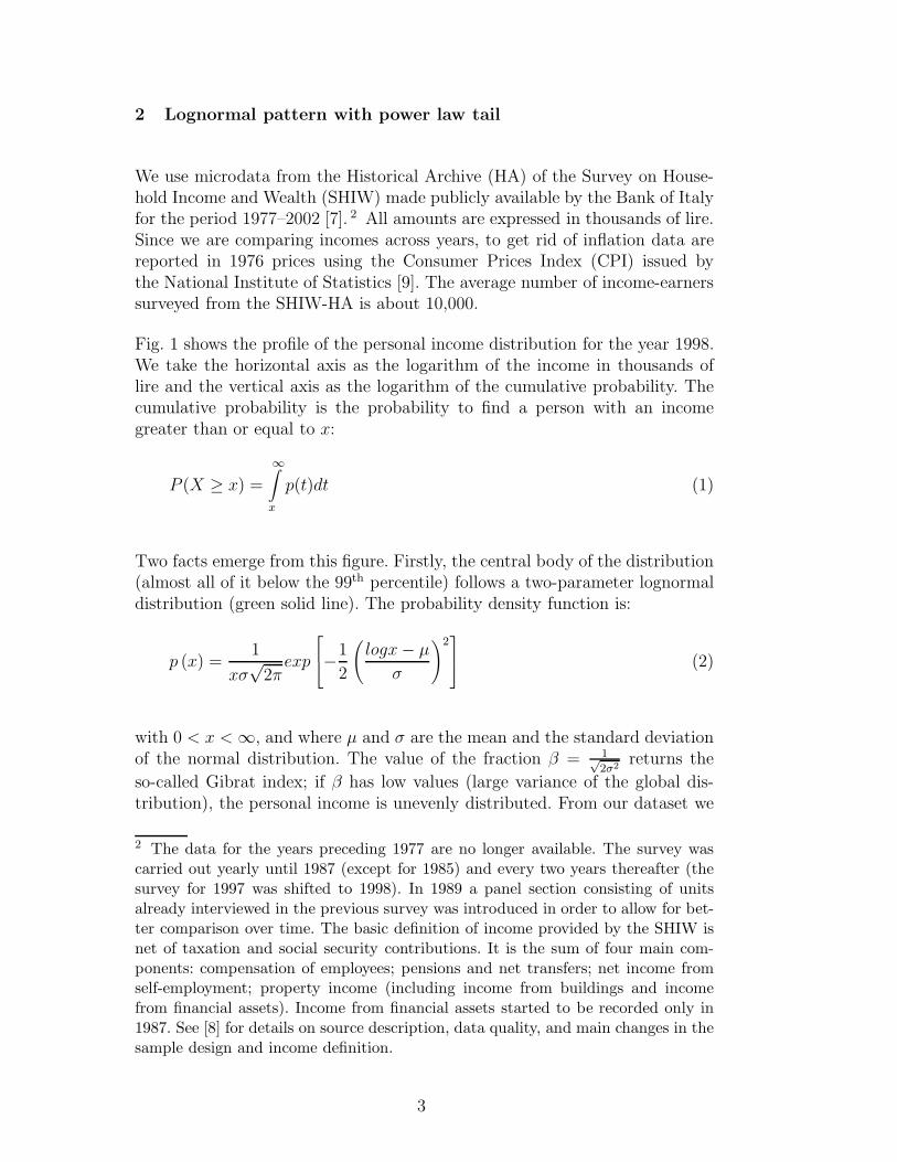
Fig. 1 shows the profile of the personal income distribution for the year 1998.We take the horizontal axis as the logarithm of the income in thousands oflire and the vertical axis as the logarithm of the cumulative probability. Thecumulative probability is the probability to find a person with an incomegreater than or equal to x:

P (X ≥ x) =

∞∫

x

p(t)dt (1)

Two facts emerge from this figure. Firstly, the central body of the distribution(almost all of it below the 99th percentile) follows a two-parameter lognormaldistribution (green solid line). The probability density function is:

p (x) =1

xσ√

2πexp

−1

2

(

logx − µ

σ

)2

(2)

with 0 < x < ∞, and where µ and σ are the mean and the standard deviationof the normal distribution. The value of the fraction β = 1√

2σ2returns the

so-called Gibrat index; if β has low values (large variance of the global dis-tribution), the personal income is unevenly distributed. From our dataset we

2 The data for the years preceding 1977 are no longer available. The survey wascarried out yearly until 1987 (except for 1985) and every two years thereafter (thesurvey for 1997 was shifted to 1998). In 1989 a panel section consisting of unitsalready interviewed in the previous survey was introduced in order to allow for bet-ter comparison over time. The basic definition of income provided by the SHIW isnet of taxation and social security contributions. It is the sum of four main com-ponents: compensation of employees; pensions and net transfers; net income fromself-employment; property income (including income from buildings and incomefrom financial assets). Income from financial assets started to be recorded only in1987. See [8] for details on source description, data quality, and main changes in thesample design and income definition.

3

Fig. 1. The cumulative probability distribution of the Italian personal income in1998. We take the horizontal axis as the logarithm of the personal income in thou-sands of lire and the vertical axis as the logarithm of the cumulative probability.The green solid line is the lognormal fit with µ = 3.48 (0.004) and σ = 0.34 (0.006).Gibrat index is β = 2.10.

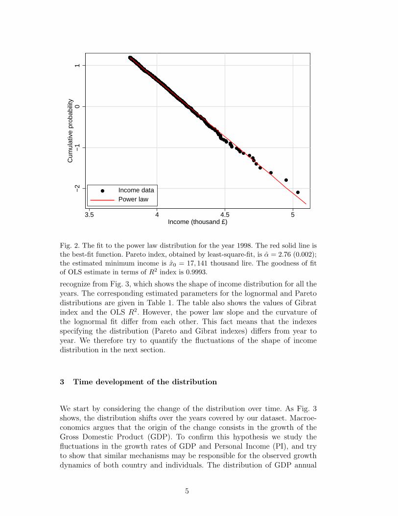
obtain the following maximum-likelihood estimates: 3 µ = 3.48 (0.004) andσ = 0.34 (0.006); 4 Gibrat index is β = 2.10. Secondly, about the top 1%of the distribution follows a Pareto (power law) distribution. This power lawbehaviour of the tail of the distribution is more evident from Fig. 2, where thered solid line is the best-fit linear function. We extract the power law slope(Pareto index) by running a simple OLS regression of the logarithm of thecumulative probability on a constant and the logarithm of personal income,obtaining a point estimate of α = 2.76 (0.002). Given this value for α, ourestimate of x0 (the income level below which the Pareto distribution wouldnot apply) is 17,141 thousand lire. The fit of linear regression is extremelygood, as one can appreciate by noting that the value of R2 index is 0.9993.

The distribution pattern of the personal income expressed as the lognormalwith power law tails seems to hold all over our time span, as one can easily

3 We exclude from our estimates about the top 1.4% of the distribution, whichbehaves as outlier, and about the bottom 0.8%, which corresponds to non positiveentries.4 The number in parentheses following a point estimate represents its standarderror.

4

−2

−1

01

Cum

ulat

ive

prob

abili

ty

3.5 4 4.5 5Income (thousand £)

Income dataPower law

Fig. 2. The fit to the power law distribution for the year 1998. The red solid line isthe best-fit function. Pareto index, obtained by least-square-fit, is α = 2.76 (0.002);the estimated minimum income is x0 = 17, 141 thousand lire. The goodness of fitof OLS estimate in terms of R2 index is 0.9993.

recognize from Fig. 3, which shows the shape of income distribution for all theyears. The corresponding estimated parameters for the lognormal and Paretodistributions are given in Table 1. The table also shows the values of Gibratindex and the OLS R2. However, the power law slope and the curvature ofthe lognormal fit differ from each other. This fact means that the indexesspecifying the distribution (Pareto and Gibrat indexes) differs from year toyear. We therefore try to quantify the fluctuations of the shape of incomedistribution in the next section.

3 Time development of the distribution

We start by considering the change of the distribution over time. As Fig. 3shows, the distribution shifts over the years covered by our dataset. Macroe-conomics argues that the origin of the change consists in the growth of theGross Domestic Product (GDP). To confirm this hypothesis we study thefluctuations in the growth rates of GDP and Personal Income (PI), and tryto show that similar mechanisms may be responsible for the observed growthdynamics of both country and individuals. The distribution of GDP annual

5

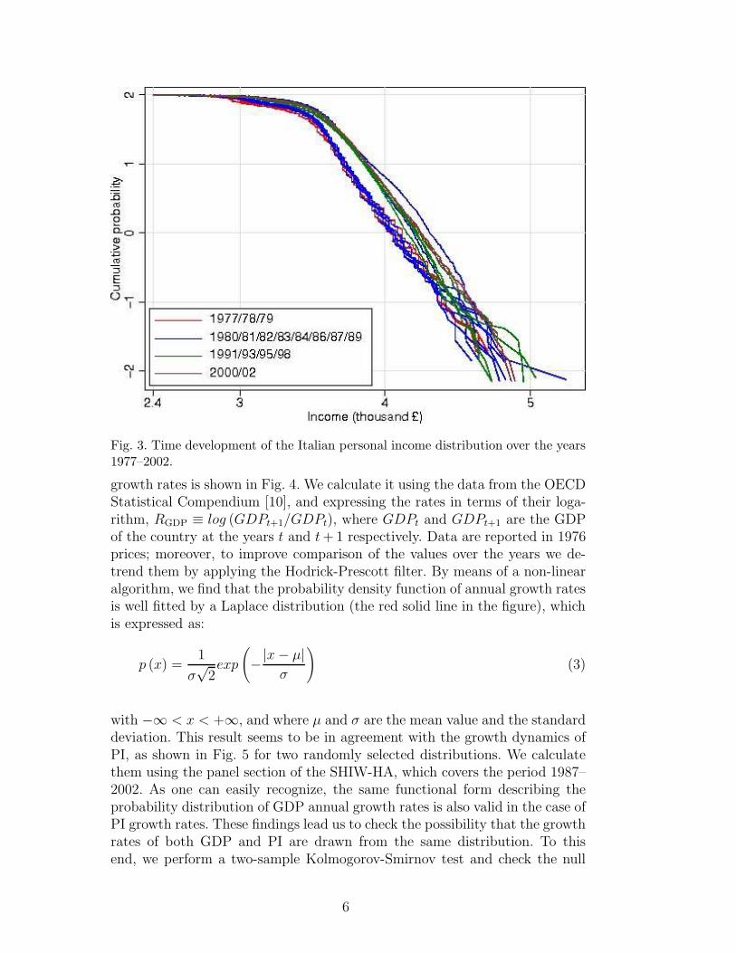
Fig. 3. Time development of the Italian personal income distribution over the years1977–2002.

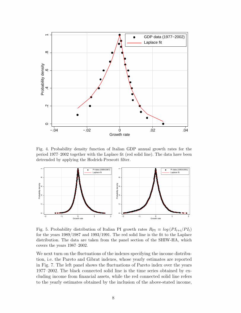
growth rates is shown in Fig. 4. We calculate it using the data from the OECDStatistical Compendium [10], and expressing the rates in terms of their loga-rithm, RGDP ≡ log (GDPt+1/GDPt), where GDPt and GDPt+1 are the GDPof the country at the years t and t + 1 respectively. Data are reported in 1976prices; moreover, to improve comparison of the values over the years we de-trend them by applying the Hodrick-Prescott filter. By means of a non-linearalgorithm, we find that the probability density function of annual growth ratesis well fitted by a Laplace distribution (the red solid line in the figure), whichis expressed as:

p (x) =1

σ√

2exp

(

−|x − µ|σ

)

(3)

with −∞ < x < +∞, and where µ and σ are the mean value and the standarddeviation. This result seems to be in agreement with the growth dynamics ofPI, as shown in Fig. 5 for two randomly selected distributions. We calculatethem using the panel section of the SHIW-HA, which covers the period 1987–2002. As one can easily recognize, the same functional form describing theprobability distribution of GDP annual growth rates is also valid in the case ofPI growth rates. These findings lead us to check the possibility that the growthrates of both GDP and PI are drawn from the same distribution. To thisend, we perform a two-sample Kolmogorov-Smirnov test and check the null

6

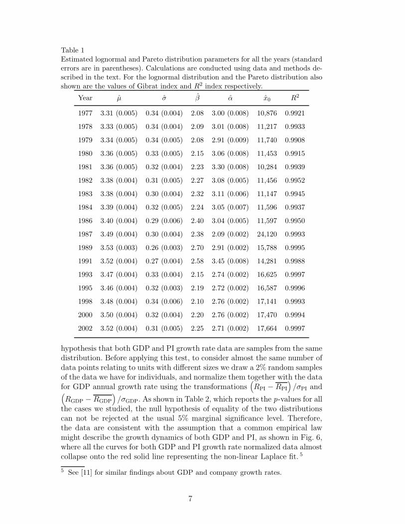
Table 1Estimated lognormal and Pareto distribution parameters for all the years (standarderrors are in parentheses). Calculations are conducted using data and methods de-scribed in the text. For the lognormal distribution and the Pareto distribution alsoshown are the values of Gibrat index and R2 index respectively.

Year µ σ β α x0 R2

1977 3.31 (0.005) 0.34 (0.004) 2.08 3.00 (0.008) 10,876 0.9921

1978 3.33 (0.005) 0.34 (0.004) 2.09 3.01 (0.008) 11,217 0.9933

1979 3.34 (0.005) 0.34 (0.005) 2.08 2.91 (0.009) 11,740 0.9908

1980 3.36 (0.005) 0.33 (0.005) 2.15 3.06 (0.008) 11,453 0.9915

1981 3.36 (0.005) 0.32 (0.004) 2.23 3.30 (0.008) 10,284 0.9939

1982 3.38 (0.004) 0.31 (0.005) 2.27 3.08 (0.005) 11,456 0.9952

1983 3.38 (0.004) 0.30 (0.004) 2.32 3.11 (0.006) 11,147 0.9945

1984 3.39 (0.004) 0.32 (0.005) 2.24 3.05 (0.007) 11,596 0.9937

1986 3.40 (0.004) 0.29 (0.006) 2.40 3.04 (0.005) 11,597 0.9950

1987 3.49 (0.004) 0.30 (0.004) 2.38 2.09 (0.002) 24,120 0.9993

1989 3.53 (0.003) 0.26 (0.003) 2.70 2.91 (0.002) 15,788 0.9995

1991 3.52 (0.004) 0.27 (0.004) 2.58 3.45 (0.008) 14,281 0.9988

1993 3.47 (0.004) 0.33 (0.004) 2.15 2.74 (0.002) 16,625 0.9997

1995 3.46 (0.004) 0.32 (0.003) 2.19 2.72 (0.002) 16,587 0.9996

1998 3.48 (0.004) 0.34 (0.006) 2.10 2.76 (0.002) 17,141 0.9993

2000 3.50 (0.004) 0.32 (0.004) 2.20 2.76 (0.002) 17,470 0.9994

2002 3.52 (0.004) 0.31 (0.005) 2.25 2.71 (0.002) 17,664 0.9997

hypothesis that both GDP and PI growth rate data are samples from the samedistribution. Before applying this test, to consider almost the same number ofdata points relating to units with different sizes we draw a 2% random samplesof the data we have for individuals, and normalize them together with the datafor GDP annual growth rate using the transformations

(

RPI − RPI

)

/σPI and(

RGDP − RGDP

)

/σGDP. As shown in Table 2, which reports the p-values for allthe cases we studied, the null hypothesis of equality of the two distributionscan not be rejected at the usual 5% marginal significance level. Therefore,the data are consistent with the assumption that a common empirical lawmight describe the growth dynamics of both GDP and PI, as shown in Fig. 6,where all the curves for both GDP and PI growth rate normalized data almostcollapse onto the red solid line representing the non-linear Laplace fit. 5

5 See [11] for similar findings about GDP and company growth rates.

7

0.2

.4.6

.81

Pro

babi

lity

dens

ity

−.04 −.02 0 .02 .04Growth rate

GDP data (1977−2002)Laplace fit

Fig. 4. Probability density function of Italian GDP annual growth rates for theperiod 1977–2002 together with the Laplace fit (red solid line). The data have beendetrended by applying the Hodrick-Prescott filter.

0.2

.4.6

.81

Pro

babi

lity

dens

ity

−2 −1 0 1 2Growth rate

PI data (1989/1987)Laplace fit

0.2

.4.6

.81

Pro

babi

lity

dens

ity

−2 −1 0 1 2Growth rate

PI data (1993/1991)Laplace fit

Fig. 5. Probability distribution of Italian PI growth rates RPI ≡ log (PIt+i/PIt)for the years 1989/1987 and 1993/1991. The red solid line is the fit to the Laplacedistribution. The data are taken from the panel section of the SHIW-HA, whichcovers the years 1987–2002.

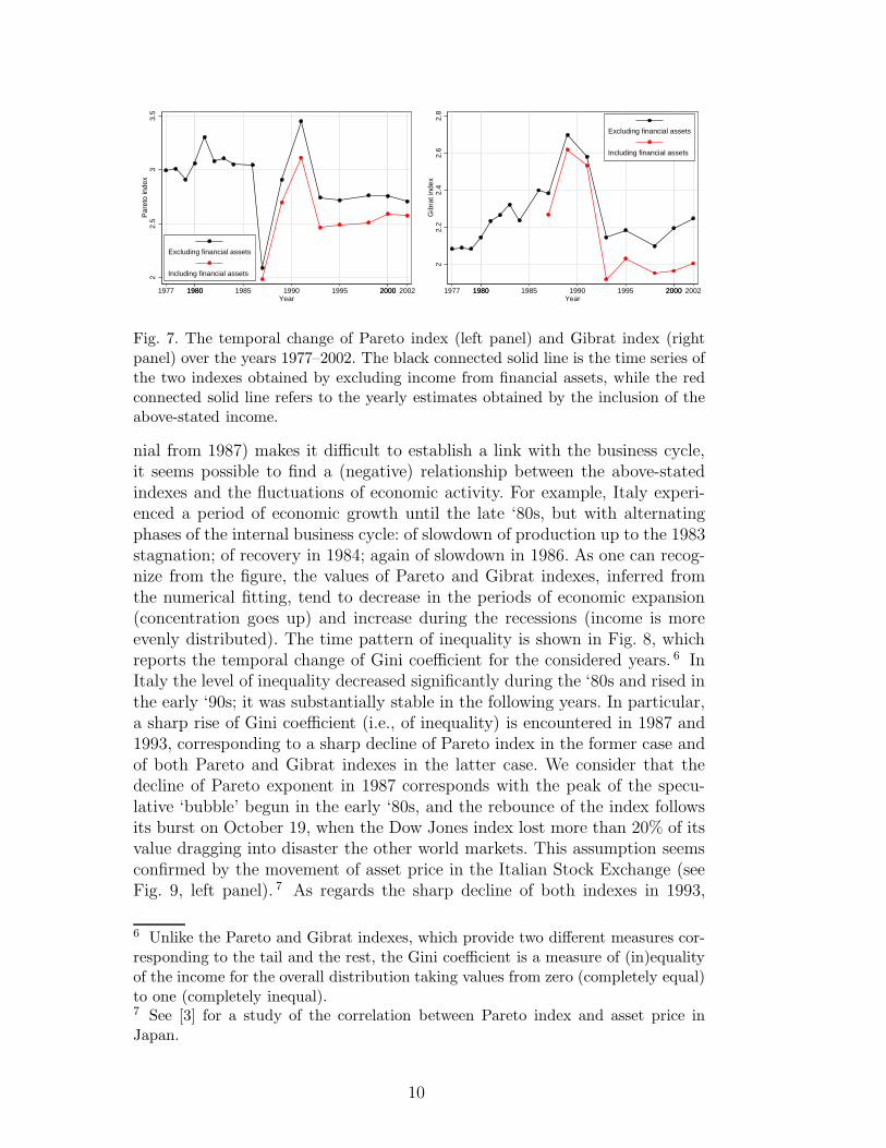
We next turn on the fluctuations of the indexes specifying the income distribu-tion, i.e. the Pareto and Gibrat indexes, whose yearly estimates are reportedin Fig. 7. The left panel shows the fluctuations of Pareto index over the years1977–2002. The black connected solid line is the time series obtained by ex-cluding income from financial assets, while the red connected solid line refersto the yearly estimates obtained by the inclusion of the above-stated income,

8

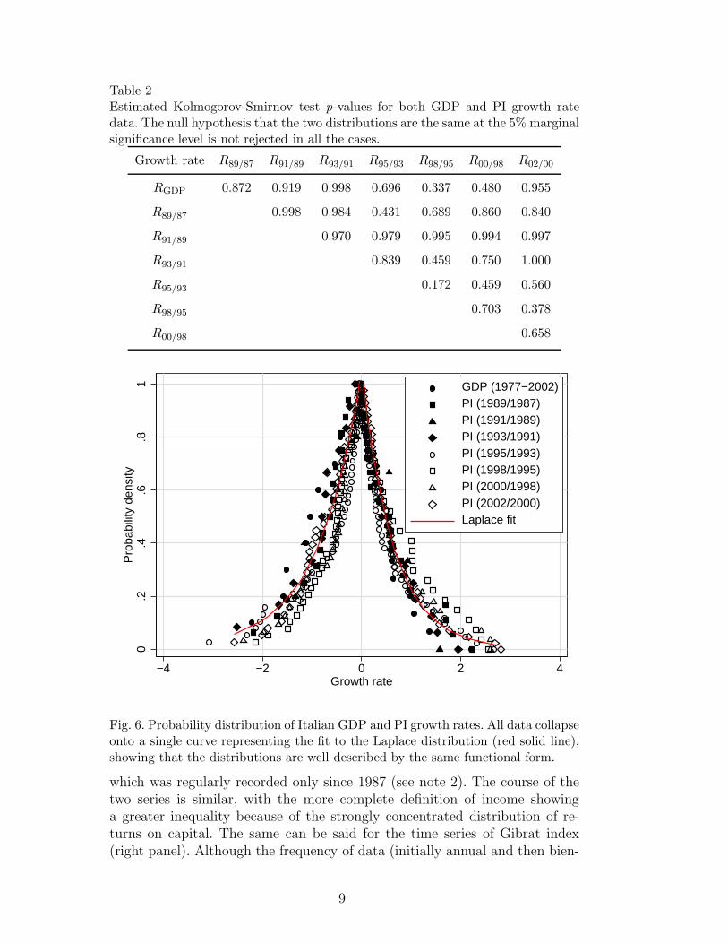
Table 2Estimated Kolmogorov-Smirnov test p-values for both GDP and PI growth ratedata. The null hypothesis that the two distributions are the same at the 5% marginalsignificance level is not rejected in all the cases.

Growth rate R89/87 R91/89 R93/91 R95/93 R98/95 R00/98 R02/00

RGDP 0.872 0.919 0.998 0.696 0.337 0.480 0.955

R89/87 0.998 0.984 0.431 0.689 0.860 0.840

R91/89 0.970 0.979 0.995 0.994 0.997

R93/91 0.839 0.459 0.750 1.000

R95/93 0.172 0.459 0.560

R98/95 0.703 0.378

R00/98 0.658

0.2

.4.6

.81

Pro

babi

lity

dens

ity

−4 −2 0 2 4Growth rate

GDP (1977−2002)PI (1989/1987)PI (1991/1989)PI (1993/1991)PI (1995/1993)PI (1998/1995)PI (2000/1998)PI (2002/2000)Laplace fit

Fig. 6. Probability distribution of Italian GDP and PI growth rates. All data collapseonto a single curve representing the fit to the Laplace distribution (red solid line),showing that the distributions are well described by the same functional form.

which was regularly recorded only since 1987 (see note 2). The course of thetwo series is similar, with the more complete definition of income showinga greater inequality because of the strongly concentrated distribution of re-turns on capital. The same can be said for the time series of Gibrat index(right panel). Although the frequency of data (initially annual and then bien-

9

22.

53

3.5

Par

eto

inde

x

1977 19801980 1985 1990 1995 20002000 2002Year

Excluding financial assets

Including financial assets

22.

22.

42.

62.

8G

ibra

t ind

ex

1977 19801980 1985 1990 1995 20002000 2002Year

Excluding financial assets

Including financial assets

Fig. 7. The temporal change of Pareto index (left panel) and Gibrat index (rightpanel) over the years 1977–2002. The black connected solid line is the time series ofthe two indexes obtained by excluding income from financial assets, while the redconnected solid line refers to the yearly estimates obtained by the inclusion of theabove-stated income.

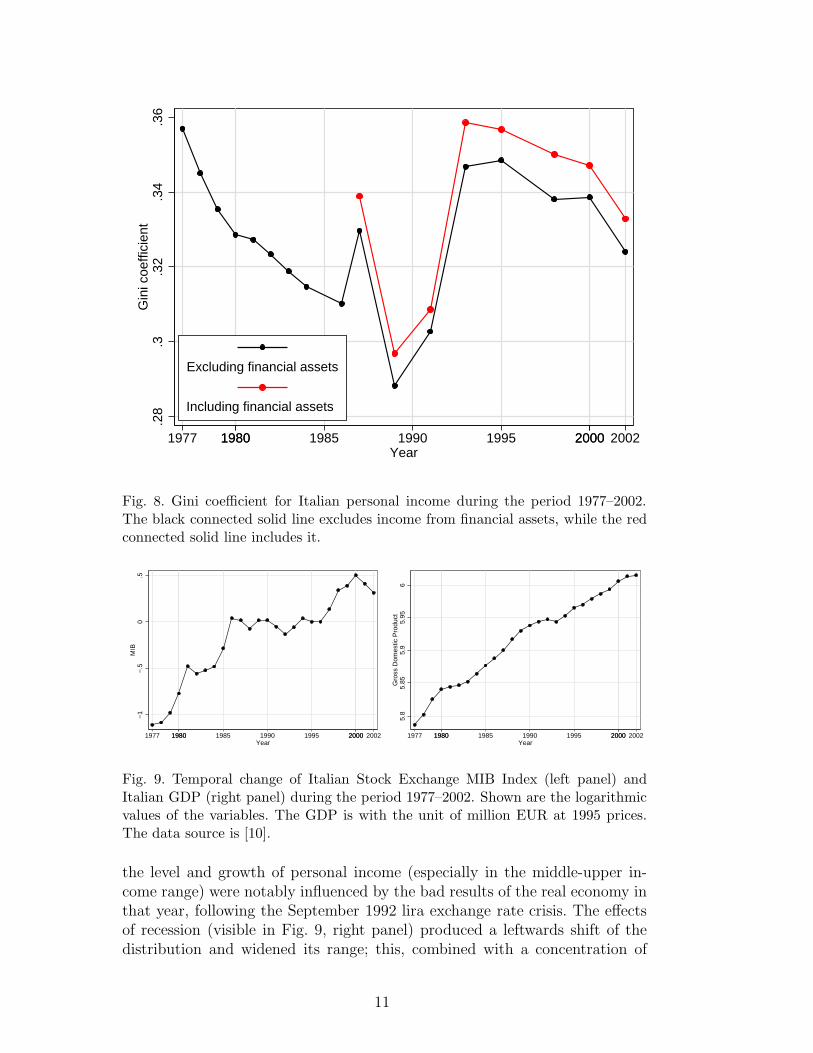
nial from 1987) makes it difficult to establish a link with the business cycle,it seems possible to find a (negative) relationship between the above-statedindexes and the fluctuations of economic activity. For example, Italy experi-enced a period of economic growth until the late ‘80s, but with alternatingphases of the internal business cycle: of slowdown of production up to the 1983stagnation; of recovery in 1984; again of slowdown in 1986. As one can recog-nize from the figure, the values of Pareto and Gibrat indexes, inferred fromthe numerical fitting, tend to decrease in the periods of economic expansion(concentration goes up) and increase during the recessions (income is moreevenly distributed). The time pattern of inequality is shown in Fig. 8, whichreports the temporal change of Gini coefficient for the considered years. 6 InItaly the level of inequality decreased significantly during the ‘80s and rised inthe early ‘90s; it was substantially stable in the following years. In particular,a sharp rise of Gini coefficient (i.e., of inequality) is encountered in 1987 and1993, corresponding to a sharp decline of Pareto index in the former case andof both Pareto and Gibrat indexes in the latter case. We consider that thedecline of Pareto exponent in 1987 corresponds with the peak of the specu-lative ‘bubble’ begun in the early ‘80s, and the rebounce of the index followsits burst on October 19, when the Dow Jones index lost more than 20% of itsvalue dragging into disaster the other world markets. This assumption seemsconfirmed by the movement of asset price in the Italian Stock Exchange (seeFig. 9, left panel). 7 As regards the sharp decline of both indexes in 1993,

6 Unlike the Pareto and Gibrat indexes, which provide two different measures cor-responding to the tail and the rest, the Gini coefficient is a measure of (in)equalityof the income for the overall distribution taking values from zero (completely equal)to one (completely inequal).7 See [3] for a study of the correlation between Pareto index and asset price inJapan.

10

.28

.3.3

2.3

4.3

6G

ini c

oeffi

cien

t

1977 19801980 1985 1990 1995 20002000 2002Year

Excluding financial assets

Including financial assets

Fig. 8. Gini coefficient for Italian personal income during the period 1977–2002.The black connected solid line excludes income from financial assets, while the redconnected solid line includes it.

−1

−.5

0.5

MIB

1977 19801980 1985 1990 1995 20002000 2002Year

5.8

5.85

5.9

5.95

6G

ross

Dom

estic

Pro

duct

1977 19801980 1985 1990 1995 20002000 2002Year

Fig. 9. Temporal change of Italian Stock Exchange MIB Index (left panel) andItalian GDP (right panel) during the period 1977–2002. Shown are the logarithmicvalues of the variables. The GDP is with the unit of million EUR at 1995 prices.The data source is [10].

the level and growth of personal income (especially in the middle-upper in-come range) were notably influenced by the bad results of the real economy inthat year, following the September 1992 lira exchange rate crisis. The effectsof recession (visible in Fig. 9, right panel) produced a leftwards shift of thedistribution and widened its range; this, combined with a concentration of

11

−2

−1

01

2C

umul

ativ

e pr

obab

ility

3.5 4 4.5 5Income (thousand £)

Income dataPower law −

2−

10

1C

umul

ativ

e pr

obab

ility

3.5 4 4.5 5Income (thousand £)

Income dataPower law

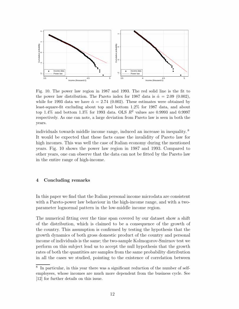
Fig. 10. The power law region in 1987 and 1993. The red solid line is the fit tothe power law distribution. The Pareto index for 1987 data is α = 2.09 (0.002),while for 1993 data we have α = 2.74 (0.002). These estimates were obtained byleast-square-fit excluding about top and bottom 1.2% for 1987 data, and abouttop 1.4% and bottom 1.3% for 1993 data. OLS R2 values are 0.9993 and 0.9997respectively. As one can note, a large deviation from Pareto law is seen in both theyears.

individuals towards middle income range, induced an increase in inequality. 8

It would be expected that these facts cause the invalidity of Pareto law forhigh incomes. This was well the case of Italian economy during the mentionedyears. Fig. 10 shows the power law region in 1987 and 1993. Compared toother years, one can observe that the data can not be fitted by the Pareto lawin the entire range of high-income.

4 Concluding remarks

In this paper we find that the Italian personal income microdata are consistentwith a Pareto-power law behaviour in the high-income range, and with a two-parameter lognormal pattern in the low-middle income region.

The numerical fitting over the time span covered by our dataset show a shiftof the distribution, which is claimed to be a consequence of the growth ofthe country. This assumption is confirmed by testing the hypothesis that thegrowth dynamics of both gross domestic product of the country and personalincome of individuals is the same; the two-sample Kolmogorov-Smirnov test weperform on this subject lead us to accept the null hypothesis that the growthrates of both the quantities are samples from the same probability distributionin all the cases we studied, pointing to the existence of correlation between

8 In particular, in this year there was a significant reduction of the number of self-employees, whose incomes are much more dependent from the business cycle. See[12] for further details on this issue.

12

them.

Moreover, by calculating the yearly estimates of Pareto and Gibrat indexes,we quantify the fluctuations of the shape of the distribution over time by es-tablishing some links with the business cycle phases which Italian economyexperienced over the years of our concern. We find that there exists a neg-ative relationship between the above-stated indexes and the fluctuations ofeconomic activity at least until the late ‘80s. In particular, we show that intwo circumstances (the 1987 burst of the asset-inflation ‘bubble’ begun in theearly ‘80s and the 1993 recession year) the data can not be fitted by a powerlaw in the entire high-income range, causing breakdown of Pareto law.

Acknowledgements

The authors would like to thank Corrado Di Guilmi and Yoshi Fujiwara forhelpful comments and suggestions.

References

[1] H. Aoyama, Y. Nagahara, M.P. Okazaki, W. Souma, H. Takayasu, and M.Takayasu (2000), Pareto’s Law for Income of Individuals and Debt of Bankrupt

Companies, Fractals, 8, 3, 293–300.

[2] E.W. Montroll, and M.F. Shlesinger (1983), Maximum Entropy Formalism,

Fractals, Scaling Phenomena, and 1/f Noise: A Tale of Tails, Journal ofStatistical Physics, 32, 2, 209–230.

[3] W. Souma (2001), Universal Structure of the Personal Income Distribution,Fractals, 9, 4, 463–470.

[4] M. Nirei, and W. Souma (2004), Two Factors Model of Income

Distribution Dynamics, paper prepared for the 9th Workshop on Economicswith Heterogeneous Agents (WEHIA), Kyoto, Japan, May 27–29, 2004,http://cmwww01.nda.ac.jp/cs/All/wehia04.

[5] A.A. Dragulescu, and V.M. Yakovenko (2001), Exponential and Power-Law

Probability Distributions of Wealth and Income in the United Kingdom and

the United States, Physica A, 299, 1–2, 213–221.

[6] W.J. Reed (2003), The Pareto Law of Incomes – An Explanation and an

Extension, Physica A, 319, 469–486.

[7] Bank of Italy, Survey on Household Income and Wealth,http://www.bancaditalia.it.

13

[8] A. Brandolini (1999), The Distribution of Personal Income in Post-War Italy:

Source Description, Data Quality, and the Time Pattern of Income Inequality,Temi di discussione n. 350, Bank of Italy, Rome.

[9] National Institute of Statistics, ConIstat, http://www.istat.it.

[10] Organisation for Economic Co-operation and Development, OECD Statistical

Compendium, ed. 02#2003.

[11] Y. Lee, L.A.N. Amaral, D. Canning, M. Meyer, and H.E. Stanley (1998),Universal Features in the Growth Dynamics of Complex Organizations, PhysicalReview Letters, 81, 15, 3275–3278.

[12] Bank of Italy (1993), Italian Household Budgets in 1993, Supplements to theStatistical Bullettin, n. 44, Rome.

14