arX

iv:g

r-qc

/040

3018

v2 2

6 A

ug 2

004

Universality of massive scalar field late-time tails in black-hole spacetimes

Lior M. BurkoDepartment of Physics, University of Utah, Salt Lake City, Utah 84112

and Gaurav KhannaPhysics Department, University of Massachusetts at Dartmouth, North Dartmouth, Massachusetts 02747

Natural Science Division, Southampton College of Long Island University, Southampton, New York 11968

(Dated: February 7, 2008)

The late-time tails of a massive scalar field in the spacetime of black holes are studied numerically.Previous analytical results for a Schwarzschild black hole are confirmed: The late-time behavior ofthe field as recorded by a static observer is given by ψ(t) ∼ t−5/6 sin[ω(t) × t], where ω(t) dependsweakly on time. This result is carried over to the case of a Kerr black hole. In particular, it is foundthat the power-law index of −5/6 depends on neither the multipole mode ℓ nor on the spin rateof the black hole a/M . In all black hole spacetimes, massive scalar fields have the same late-timebehavior irrespective of their initial data (i.e., angular distribution). Their late-time behavior isuniversal.

PACS numbers: 04.30.Nk, 04.70.Bw, 04.25.Dm

I. INTRODUCTION

The late-time behavior of massless fields in black hole spacetime has been studied in detail for both linearized [1, 2]and fully nonlinear (spherical) evolutions [3, 4]. In contrast, the late-time behavior of massive fields has been studiedin much less detail. In this paper we study the late-time behavior of a scalar field numerically, in the spacetimes ofSchwarzschild and Kerr black holes.

The first to consider the problem of a massive scalar field in the spacetime of a Schwarzschild black hole wereNovikov and Starobinski, who studied the problem in the frequency domain, and found that there are poles in thecomplex plane closer to the real axis than in the massless case. They thus inferred that the decay rate would be slowerin the massive case than in the massless case [5]. That problem was later studied numerically by Burko [6] both fora linearized massive scalar field, and for a self-gravitating, spherical massive field. In both cases it was found in [6]that the late-time behavior was given by an oscillating field, whose envelope decayed according to an inverse powerlaw, and whose frequency was determined by the Compton wavelength of the field, i.e., by its mass term. In [6] itwas also reported that the decay rate of the envelope was given by t−α, where α ∼ 0.8. No attempt was done in [6],however, to determine the value of α accurately, or to determine its dependence or lack thereof of the parameters ofthe problem. The most detailed analytical study of the problem was done by Koyama and Tomimatsu in a series ofthree papers [7, 8, 9].

The most striking feature of the problem of tails of a massive scalar field is that the tails exist already in flatspacetime [11], because spacetime acts like a dispersive medium for a Klein-Gordon field. Based on the exact Greenfunction, the behavior of the field in Minkowski spacetime was found in [6] to be given by

ψflat ∼ t−ℓ−3/2 sin(µt) , (1.1)

ℓ being the multipole moment of the field, and µ−1 being its Compton wavelength. A derivation of Eq. (1.1) appearsin the Appendix. More recently, an interesting self similar behavior of a Klein-Gordon field in Minkowski spacetimewas found in [10]. The self similar behavior reduces to Eq. (1.1) for a field evaluated at a fixed location at very latetimes.

In the spacetime of a Schwarzschild black hole there are important differences. The decay rate was found in [8] tobe given by

ψsch ∼ t−5/6 sin[ω(t) × t] , (1.2)

where the power index is independent of ℓ. The time-evolving angular frequency ω(t) approaches µ asymptotically ast→ ∞, but is different from µ at finite values of time. This result was generalized in [9] to any spherically symmetric,static black hole spacetime. The details of this result have not been corroborated numerically—although qualitativelythey are supported by the results of [6]—a task we undertake in this paper. In addition, we also show that this resultremains correct also for a Kerr black hole, for which the power index −5/6 is independent of both ℓ and the spin rateof the black hole a/M . We also study the behavior of ω(t), and find it to be in agreement with the results of [8, 9].Similar conclusions were obtained recently also for a spinning dilaton black hole [12] (see also [13]).

2

II. MASSIVE TAILS IN SCHWARZSCHILD SPACETIME

Massive fields in Schwarzschild spacetime were studied numerically (for both a linearized and for a spherical self-gravitating Klein-Gordon field) in [6] and analytically in [8]. As discussed in [8], for µM . 1, the tail regime satisfiest≫ µ−3M−2, M being the mass of the black hole, and t being the regular Schwarzschild time coordinate. Therefore,for a light scalar field, the heavier the field is, the earlier the tails are seen. (For heavy fields, µM ≫ 1, the tail regimeis for t ≫ M , independently of the mass of the field.) To facilitate numerical simulations, one is tempted then toincrease the mass of the field. However, increasing the mass of the scalar field requires also to increase the resolution,as the wavelength of the field is inversely proportional to its mass, and as one needs at least a few data points perwavelength to resolve an oscillating field. One faces then a competing effect: to decrease the computational time toan optimum one needs to balance the scalar field mass and the resolution of the numerical code. (We do not discusshere the case of µM ≫ 1 as the required numerical resolution is beyond current practical computational limits.) Onemay gain insight into the above discussion, noticing, following [6], that for µ ≪ 1/M , the corresponding Comptonwavelength of the scalar field λ(= µ−1) ≫ M , that is the field’s wavelength is much longer than the typical radiusof curvature of spacetime, or the scale of inhomogeneity of curvature. We therefore expect the field at early times toevolve similarly to its evolution in flat spacetime. At later times the curvature effects become apparent, and we expectdeviations from the flat-spacetime behavior. At asymptotically late times we expect to find the behavior predicted in[8]. The greater the mass term µ, the shorter the associated Compton wavelength λ, and the sooner the asymptoticdomain is expected. We therefore expect an oscillating field, whose envelope is a broken power law: at early times itis described by t−ℓ−3/2 and at late times by t−5/6.

The field ψ satisfies the Klein-Gordon equation

(� − µ2)φ = 0 , (2.1)

� being the D’Alembertian operator in curved spacetime. We define ψ = rφ in the usual way, and decompose thefield ψ into Legendre modes ψ =

∑

ℓ ψℓPℓ(cos θ). The radial equation that each mode ψℓ satisfies is then given by

ψℓ,uv +

1

4Vℓ(r)ψ

ℓ = 0 , (2.2)

where the effective potential

Vℓ(r) =

(

1 − 2M

r

) [

ℓ(ℓ+ 1)

r2+

2M

r3+ µ2

]

. (2.3)

To test our expectations in the context of a Schwarzschild black hole, we used a double-null code in 1+1D, andsolved the radial equation for ψℓ. We specified a pulse of the form

ψℓ(u) =

[

4(u− u1)(u− u2)

(u2 − u1)2

]8

(2.4)

along the ingoing segment of the characteristic hypersurface v = 0 for u1 < u < u2, and ψ(u) = 0 otherwise. Wealso took ψ(v) = 0 along u = 0. Here, u (v) is the usual retarded (advanced) time. The results reported on belowcorrespond to u1 = 20M and u2 = 60M , but our results are unchanged also for other choices of the parameters, orfor other choices of the characteristic pulse. In the following we observe the fields along r∗ = 0, r∗ being the usualRegge-Wheeler ‘tortoise’ coordinate.

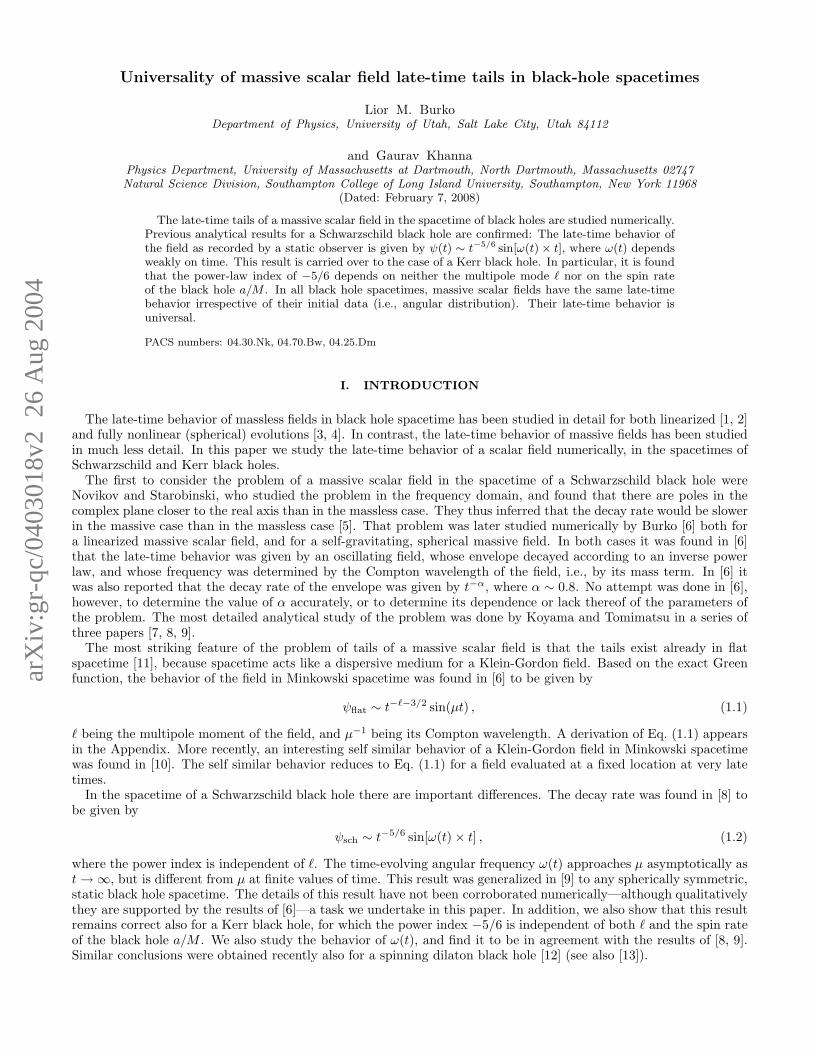
The code is stable, and exhibits second order convergence. The convergence test is presented in Fig. 1, which showsthe ratio of differences for three runs with different resolutions.

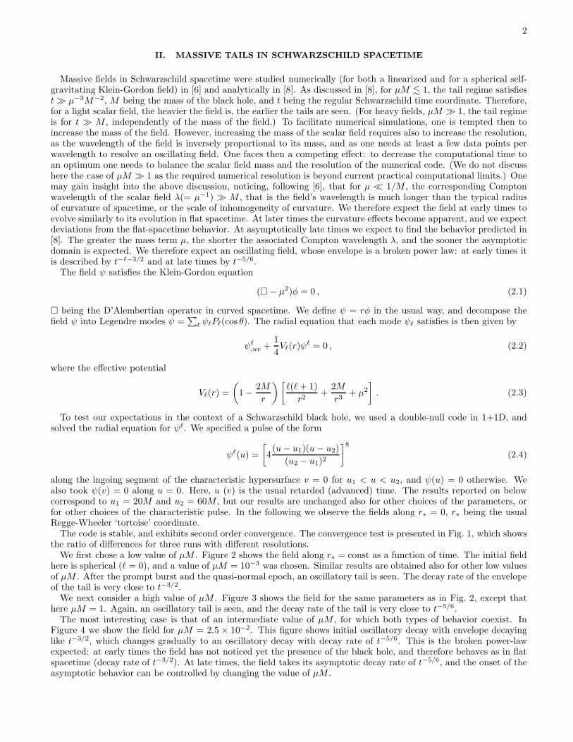
We first chose a low value of µM . Figure 2 shows the field along r∗ = const as a function of time. The initial fieldhere is spherical (ℓ = 0), and a value of µM = 10−3 was chosen. Similar results are obtained also for other low valuesof µM . After the prompt burst and the quasi-normal epoch, an oscillatory tail is seen. The decay rate of the envelopeof the tail is very close to t−3/2.

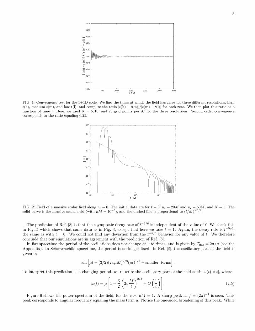
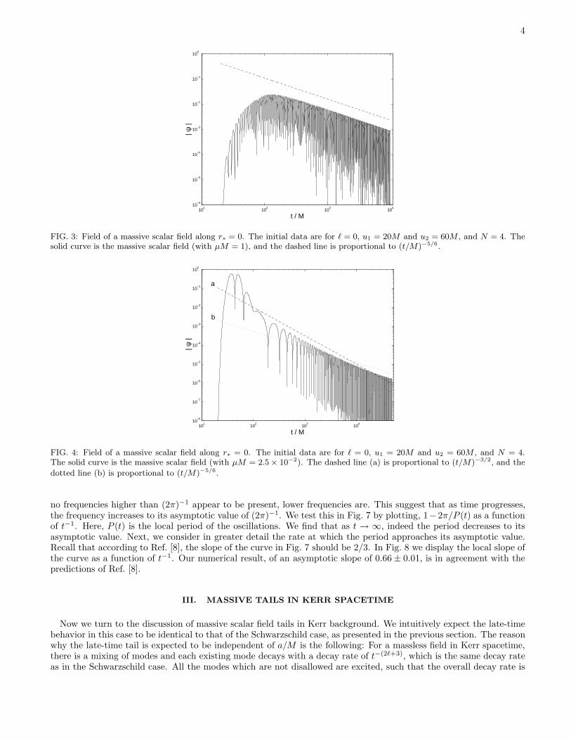
We next consider a high value of µM . Figure 3 shows the field for the same parameters as in Fig. 2, except thathere µM = 1. Again, an oscillatory tail is seen, and the decay rate of the tail is very close to t−5/6.

The most interesting case is that of an intermediate value of µM , for which both types of behavior coexist. InFigure 4 we show the field for µM = 2.5 × 10−2. This figure shows initial oscillatory decay with envelope decayinglike t−3/2, which changes gradually to an oscillatory decay with decay rate of t−5/6. This is the broken power-lawexpected: at early times the field has not noticed yet the presence of the black hole, and therefore behaves as in flatspacetime (decay rate of t−3/2). At late times, the field takes its asymptotic decay rate of t−5/6, and the onset of theasymptotic behavior can be controlled by changing the value of µM .

3

500 1000 1500 2000 2500 30000.24

0.242

0.244

0.246

0.248

0.25

0.252

0.254

0.256

0.258

0.26

t / M

[ t (

h) −

t (m

) ] /

[ t (

m)

− t

(l) ]

FIG. 1: Convergence test for the 1+1D code. We find the times at which the field has zeros for three different resolutions, hight(h), medium t(m), and low t(l), and compute the ratio [t(h) − t(m)]/[t(m) − t(l)] for each zero. We then plot this ratio as afunction of time t. Here, we used N = 5, 10, and 20 grid points per M for the three resolutions. Second order convergencecorresponds to the ratio equaling 0.25.

101

102

103

104

10−8

10−7

10−6

10−5

10−4

10−3

10−2

10−1

100

t / M

| ψ |

FIG. 2: Field of a massive scalar field along r∗ = 0. The initial data are for ℓ = 0, u1 = 20M and u2 = 60M , and N = 1. Thesolid curve is the massive scalar field (with µM = 10−3), and the dashed line is proportional to (t/M)−3/2.

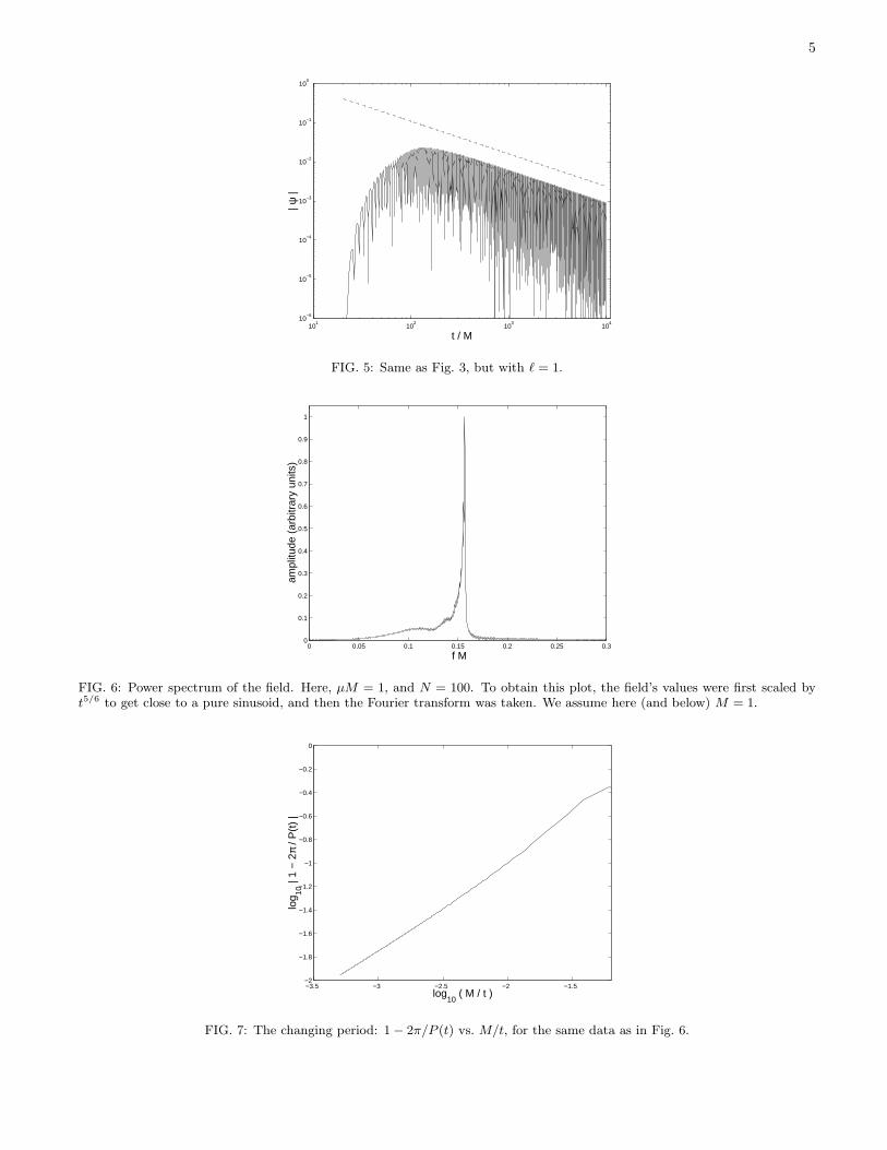
The prediction of Ref. [8] is that the asymptotic decay rate of t−5/6 is independent of the value of ℓ. We check thisin Fig. 5 which shows that same data as in Fig. 3, except that here we take ℓ = 1. Again, the decay rate is t−5/6,the same as with ℓ = 0. We could not find any deviation from the t−5/6 behavior for any value of ℓ. We thereforeconclude that our simulations are in agreement with the prediction of Ref. [8].

In flat spacetime the period of the oscillations does not change at late times, and is given by Tflat = 2π/µ (see theAppendix). In Schwarzschild spacetime, the period is no longer fixed. In Ref. [8], the oscillatory part of the field isgiven by

sin[

µt− (3/2)(2πµM)2/3(µt)1/3 + smaller terms]

.

To interpret this prediction as a changing period, we re-write the oscillatory part of the field as sin[ω(t) × t], where

ω(t) = µ

[

1 − 3

2

(

2πM

t

)2/3

+O

(

1

t

)

]

. (2.5)

Figure 6 shows the power spectrum of the field, for the case µM = 1. A sharp peak at f = (2π)−1 is seen. Thispeak corresponds to angular frequency equaling the mass term µ. Notice the one-sided broadening of this peak. While

4

101

102

103

104

10−6

10−5

10−4

10−3

10−2

10−1

100

t / M

| ψ |

FIG. 3: Field of a massive scalar field along r∗ = 0. The initial data are for ℓ = 0, u1 = 20M and u2 = 60M , and N = 4. Thesolid curve is the massive scalar field (with µM = 1), and the dashed line is proportional to (t/M)−5/6.

101

102

103

104

10−8

10−7

10−6

10−5

10−4

10−3

10−2

10−1

100

t / M

| ψ

|

a

b

FIG. 4: Field of a massive scalar field along r∗ = 0. The initial data are for ℓ = 0, u1 = 20M and u2 = 60M , and N = 4.The solid curve is the massive scalar field (with µM = 2.5 × 10−2). The dashed line (a) is proportional to (t/M)−3/2, and the

dotted line (b) is proportional to (t/M)−5/6.

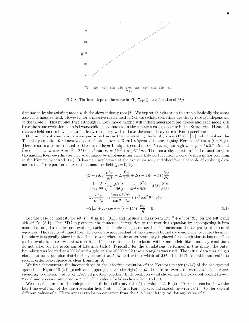
no frequencies higher than (2π)−1 appear to be present, lower frequencies are. This suggest that as time progresses,the frequency increases to its asymptotic value of (2π)−1. We test this in Fig. 7 by plotting, 1−2π/P (t) as a functionof t−1. Here, P (t) is the local period of the oscillations. We find that as t → ∞, indeed the period decreases to itsasymptotic value. Next, we consider in greater detail the rate at which the period approaches its asymptotic value.Recall that according to Ref. [8], the slope of the curve in Fig. 7 should be 2/3. In Fig. 8 we display the local slope ofthe curve as a function of t−1. Our numerical result, of an asymptotic slope of 0.66 ± 0.01, is in agreement with thepredictions of Ref. [8].

III. MASSIVE TAILS IN KERR SPACETIME

Now we turn to the discussion of massive scalar field tails in Kerr background. We intuitively expect the late-timebehavior in this case to be identical to that of the Schwarzschild case, as presented in the previous section. The reasonwhy the late-time tail is expected to be independent of a/M is the following: For a massless field in Kerr spacetime,there is a mixing of modes and each existing mode decays with a decay rate of t−(2ℓ+3), which is the same decay rateas in the Schwarzschild case. All the modes which are not disallowed are excited, such that the overall decay rate is

5

101

102

103

104

10−6

10−5

10−4

10−3

10−2

10−1

100

t / M

| ψ |

FIG. 5: Same as Fig. 3, but with ℓ = 1.

0 0.05 0.1 0.15 0.2 0.25 0.30

0.1

0.2

0.3

0.4

0.5

0.6

0.7

0.8

0.9

1

f M

ampl

itude

(ar

bitr

ary

units

)

FIG. 6: Power spectrum of the field. Here, µM = 1, and N = 100. To obtain this plot, the field’s values were first scaled byt5/6 to get close to a pure sinusoid, and then the Fourier transform was taken. We assume here (and below) M = 1.

−3.5 −3 −2.5 −2 −1.5−2

−1.8

−1.6

−1.4

−1.2

−1

−0.8

−0.6

−0.4

−0.2

0

log10

( M / t )

log 10

| 1

− 2

π / P

(t)

|

FIG. 7: The changing period: 1 − 2π/P (t) vs. M/t, for the same data as in Fig. 6.

6

0 0.001 0.002 0.003 0.004 0.005 0.006 0.007 0.008 0.009 0.010.65

0.7

0.75

0.8

0.85

0.9

M / t

p(t)

FIG. 8: The local slope of the curve in Fig. 7, p(t), as a function of M/t.

dominated by the existing mode with the slowest decay rate [2]. We expect this situation to remain basically the samealso for a massive field. However, for a massive scalar field in Schwarzschild spacetime the decay rate is independentof the mode ℓ. This implies that although in Kerr mode mixing will indeed generate more modes and each mode willhave the same evolution as in Schwarzschild spacetime (as in the massless case), because in the Schwarzschild case allmassive field modes have the same decay rate, they will all have the same decay rate in Kerr spacetime.

Our numerical simulations were performed using the penetrating Teukolsky code (PTC) [14], which solves theTeukolsky equation for linearized perturbations over a Kerr background in the ingoing Kerr coordinates (t̃, r, θ, ϕ̃).These coordinates are related to the usual Boyer-Lindquist coordinates (t, r, θ, ϕ) through ϕ̃ = ϕ +

∫

a∆−1 dr and

t̃ = t− r + r∗, where ∆ = r2 − 2Mr + a2 and r∗ =∫

(r2 + a2)∆−1 dr. The Teukolsky equation for the function ψ inthe ingoing Kerr coordinates can be obtained by implementing black hole perturbation theory (with a minor rescalingof the Kinnersley tetrad [14]). It has no singularities at the event horizon, and therefore is capable of evolving dataacross it. This equation is given for a massless field (µ = 0) by

(Σ + 2Mr)∂2ψ

∂t̃2− ∆

∂2ψ

∂r2+ 2(s− 1)(r −M)

∂ψ

∂r

− 1

sin θ

∂

∂θ

(

sin θ∂ψ

∂θ

)

− 1

sin2 θ

∂2ψ

∂ϕ̃2− 4Mr

∂2ψ

∂t̃∂r

−2a∂2ψ

∂r∂ϕ̃− i

2s cot θ

sin θ

∂ψ

∂ϕ̃+ (s2 cot2 θ + s)ψ

+2 [sr + ias cos θ + (s− 1)M ]∂ψ

∂t̃= 0 . (3.1)

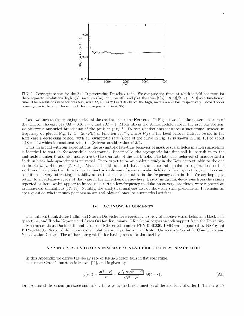
For the case of interest, we set s = 0 in Eq. (3.1), and include a mass term µ2(r2 + a2 cos2 θ)ψ on the left handside of Eq. (3.1). The PTC implements the numerical integration of the resulting equation by decomposing it intoazimuthal angular modes and evolving each such mode using a reduced 2+1 dimensional linear partial differentialequation. The results obtained from this code are independent of the choice of boundary conditions, because the innerboundary is typically placed inside the horizon, whereas the outer boundary is placed far enough that it has no effecton the evolution. (As was shown in Ref. [15], close timelike boundaries with Sommerfeld-like boundary conditionsdo not allow for the evolution of late-time tails.) Typically, for the simulations performed in this study, the outerboundary was located at 4000M and a grid of size 40000 × 32 (radial×angle) was used. The initial data was alwayschosen to be a gaussian distribution, centered at 50M and with a width of 2M . The PTC is stable and exhibitssecond order convergence as clear from Fig. 9.

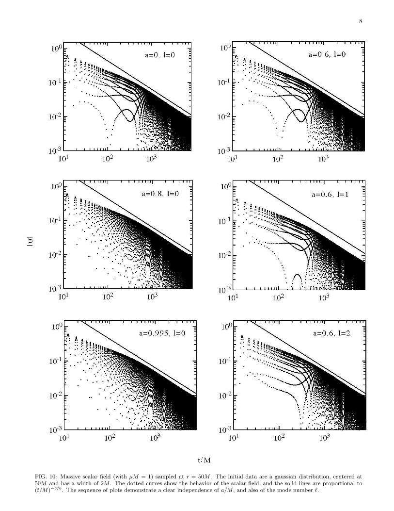
We first demonstrate the independence of the late-time evolution of the Kerr parameter (a/M) of the backgroundspacetime. Figure 10 (left panels and upper panel on the right) shows tails from several different evolutions corre-sponding to different values of a/M , all plotted together. Each oscillatory tail shown has the expected period (about2π/µ) and a decay rate close to t−5/6. The value of µM is chosen here to be 1.

We next demonstrate the independence of the oscillatory tail of the value of ℓ. Figure 10 (right panels) shows thelate-time evolution of the massive scalar field (µM = 1) in a Kerr background spacetime with a/M = 0.6 for severaldifferent values of ℓ. There appears to be no deviation from the t−5/6 oscillatory tail for any value of ℓ.

7

0 1000 2000 3000 40000.20

0.24

0.28

t/M

[t(h

)-t(

m)]

/[t(

m)-

t(l)

]

FIG. 9: Convergence test for the 2+1 D penetrating Teukolsky code. We compute the times at which is field has zeros forthree separate resolutions [high t(h), medium t(m), and low t(l)] and plot the ratio [t(h) − t(m)]/[t(m) − t(l)] as a function oftime. The resolutions used for this test, were M/40, M/20 and M/10 for the high, medium and low, respectively. Second orderconvergence is clear by the value of the convergence ratio (0.25).

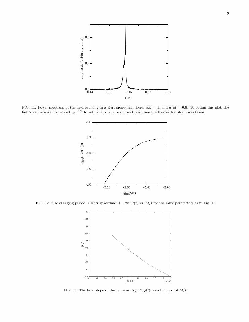
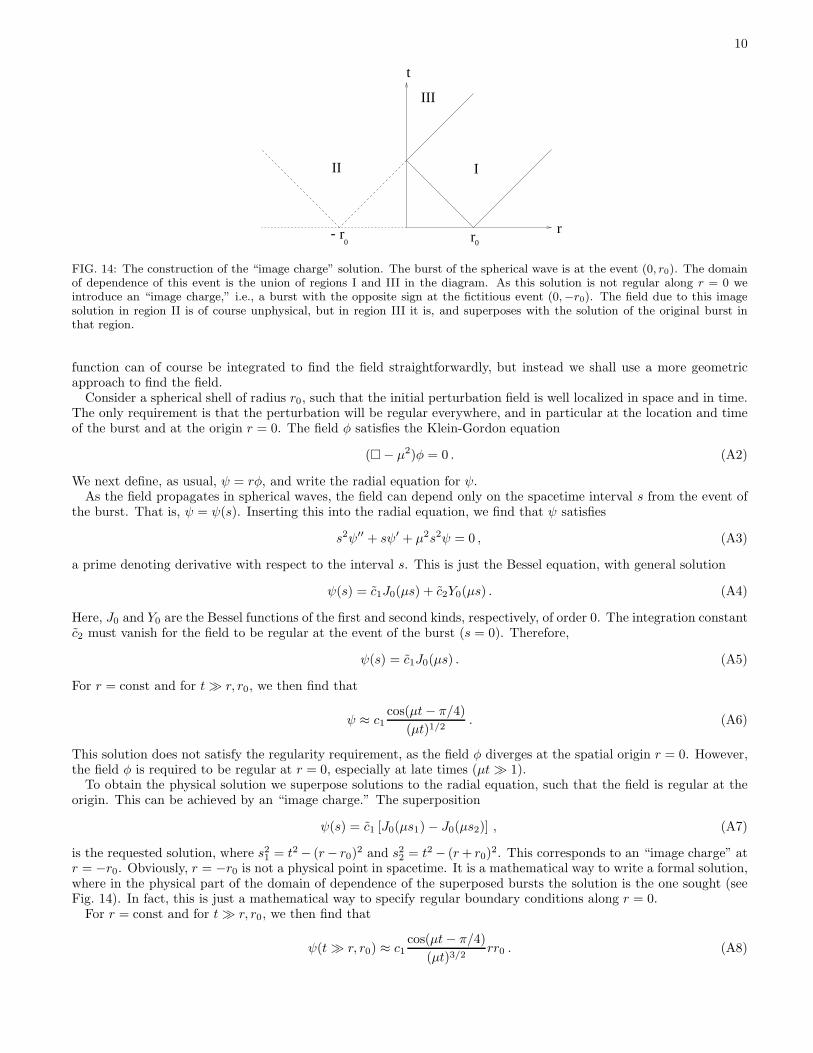
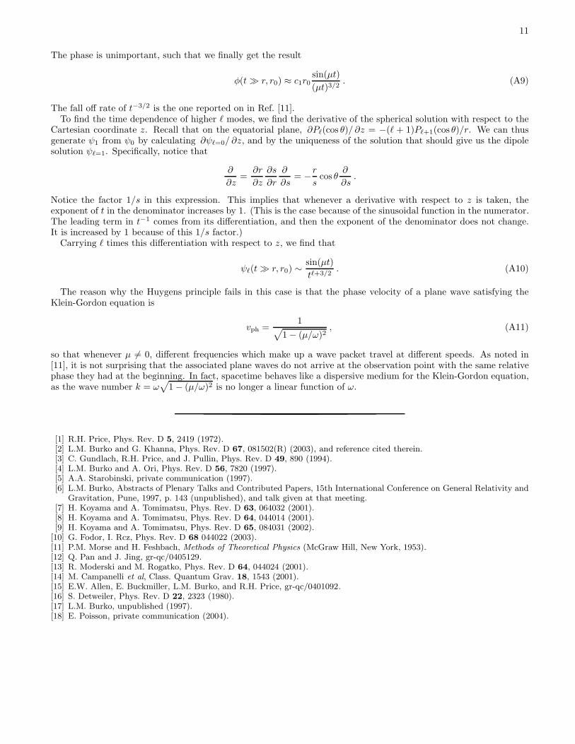
Last, we turn to the changing period of the oscillations in the Kerr case. In Fig. 11 we plot the power spectrum ofthe field for the case of a/M = 0.6, ℓ = 0 and µM = 1. Much like in the Schwarzschild case in the previous Section,we observe a one-sided broadening of the peak at (2π)−1. To test whether this indicates a monotonic increase infrequency we plot in Fig. 12, 1 − 2π/P (t) as function of t−1, where P (t) is the local period. Indeed, we see in theKerr case a decreasing period, with an asymptotic rate (slope of the curve in Fig. 12 is shown in Fig. 13) of about0.68 ± 0.02 which is consistent with the (Schwarzschild) value of 2/3.

Thus, in accord with our expectations, the asymptotic late-time behavior of massive scalar fields in a Kerr spacetimeis identical to that in Schwarzschild background. Specifically, the asymptotic late-time tail is insensitive to themultipole number ℓ, and also insensitive to the spin rate of the black hole. The late-time behavior of massive scalarfields in black hole spacetimes is universal. There is yet to be an analytic study in the Kerr context, akin to the onein the Schwarzschild case [7, 8, 9]. Also, it should be noted that all the numerical simulations reported on in thiswork were axisymmetric. In a nonaxisymmetric evolution of massive scalar fields in a Kerr spacetime, under certainconditions, a very interesting instability arises that has been studied in the frequency-domain [16]. We are hoping toreturn to an extensive study of that case in the time-domain elsewhere. Lastly, intriguing deviations from the resultsreported on here, which appear to introduce a certain low-frequency modulation at very late times, were reported onin numerical simulations [17, 18]. Notably, the analytical analyses do not show any such phenomena. It remains anopen question whether such phenomena are real physical ones, or a numerical artifact.

IV. ACKNOWLEDGEMENTS

The authors thank Jorge Pullin and Steven Detweiler for suggesting a study of massive scalar fields in a black holespacetime, and Hiroko Koyama and Amos Ori for discussions. GK acknowledges research support from the Universityof Massachusetts at Dartmouth and also from NSF grant number PHY-0140236. LMB was supported by NSF grantPHY-0244605. Some of the numerical simulations were performed at Boston University’s Scientific Computing andVisualization Center. The authors are grateful for having access to that facility.

APPENDIX A: TAILS OF A MASSIVE SCALAR FIELD IN FLAT SPACETIME

In this Appendix we derive the decay rate of Klein-Gordon tails in flat spacetime.The exact Green’s function is known [11], and is given by

g(r, t) =δ(t− r)

r− µJ1[µ

√t2 − r2]√

t2 − r2Θ(t− r) , (A1)

for a source at the origin (in space and time). Here, J1 is the Bessel function of the first king of order 1. This Green’s

8

FIG. 10: Massive scalar field (with µM = 1) sampled at r = 50M . The initial data are a gaussian distribution, centered at50M and has a width of 2M . The dotted curves show the behavior of the scalar field, and the solid lines are proportional to(t/M)−5/6. The sequence of plots demonstrate a clear independence of a/M , and also of the mode number ℓ.

9

0.14 0.15 0.16 0.17 0.180.0

0.4

0.8

f M

amp

litu

de

(arb

itra

ry u

nit

s)

FIG. 11: Power spectrum of the field evolving in a Kerr spacetime. Here, µM = 1, and a/M = 0.6. To obtain this plot, the

field’s values were first scaled by t5/6 to get close to a pure sinusoid, and then the Fourier transform was taken.

-3.20 -2.80 -2.40 -2.00-2.0

-1.9

-1.8

-1.7

-1.6

log10(M/t)

log 1

0(1-

2π/P

(t))

FIG. 12: The changing period in Kerr spacetime: 1 − 2π/P (t) vs. M/t for the same parameters as in Fig. 11

0 0.2 0.4 0.6 0.8 1 1.2 1.4 1.6 1.8 2

x 10−3

0.25

0.3

0.35

0.4

0.45

0.5

0.55

0.6

0.65

0.7

M / t

p (t

)

FIG. 13: The local slope of the curve in Fig. 12, p(t), as a function of M/t.

10

r

t

r0r-

0

III

III

FIG. 14: The construction of the “image charge” solution. The burst of the spherical wave is at the event (0, r0). The domainof dependence of this event is the union of regions I and III in the diagram. As this solution is not regular along r = 0 weintroduce an “image charge,” i.e., a burst with the opposite sign at the fictitious event (0,−r0). The field due to this imagesolution in region II is of course unphysical, but in region III it is, and superposes with the solution of the original burst inthat region.

function can of course be integrated to find the field straightforwardly, but instead we shall use a more geometricapproach to find the field.

Consider a spherical shell of radius r0, such that the initial perturbation field is well localized in space and in time.The only requirement is that the perturbation will be regular everywhere, and in particular at the location and timeof the burst and at the origin r = 0. The field φ satisfies the Klein-Gordon equation

(� − µ2)φ = 0 . (A2)

We next define, as usual, ψ = rφ, and write the radial equation for ψ.As the field propagates in spherical waves, the field can depend only on the spacetime interval s from the event of

the burst. That is, ψ = ψ(s). Inserting this into the radial equation, we find that ψ satisfies

s2ψ′′ + sψ′ + µ2s2ψ = 0 , (A3)

a prime denoting derivative with respect to the interval s. This is just the Bessel equation, with general solution

ψ(s) = c̃1J0(µs) + c̃2Y0(µs) . (A4)

Here, J0 and Y0 are the Bessel functions of the first and second kinds, respectively, of order 0. The integration constantc̃2 must vanish for the field to be regular at the event of the burst (s = 0). Therefore,

ψ(s) = c̃1J0(µs) . (A5)

For r = const and for t≫ r, r0, we then find that

ψ ≈ c1cos(µt− π/4)

(µt)1/2. (A6)

This solution does not satisfy the regularity requirement, as the field φ diverges at the spatial origin r = 0. However,the field φ is required to be regular at r = 0, especially at late times (µt ≫ 1).

To obtain the physical solution we superpose solutions to the radial equation, such that the field is regular at theorigin. This can be achieved by an “image charge.” The superposition

ψ(s) = c̃1 [J0(µs1) − J0(µs2)] , (A7)

is the requested solution, where s21 = t2 − (r− r0)2 and s22 = t2 − (r+ r0)

2. This corresponds to an “image charge” atr = −r0. Obviously, r = −r0 is not a physical point in spacetime. It is a mathematical way to write a formal solution,where in the physical part of the domain of dependence of the superposed bursts the solution is the one sought (seeFig. 14). In fact, this is just a mathematical way to specify regular boundary conditions along r = 0.

For r = const and for t≫ r, r0, we then find that

ψ(t ≫ r, r0) ≈ c1cos(µt− π/4)

(µt)3/2rr0 . (A8)

11

The phase is unimportant, such that we finally get the result

φ(t ≫ r, r0) ≈ c1r0sin(µt)

(µt)3/2. (A9)

The fall off rate of t−3/2 is the one reported on in Ref. [11].To find the time dependence of higher ℓ modes, we find the derivative of the spherical solution with respect to the

Cartesian coordinate z. Recall that on the equatorial plane, ∂Pℓ(cos θ)/ ∂z = −(ℓ + 1)Pℓ+1(cos θ)/r. We can thusgenerate ψ1 from ψ0 by calculating ∂ψℓ=0/ ∂z, and by the uniqueness of the solution that should give us the dipolesolution ψℓ=1. Specifically, notice that

∂

∂z=

∂r

∂z

∂s

∂r

∂

∂s= −r

scos θ

∂

∂s.

Notice the factor 1/s in this expression. This implies that whenever a derivative with respect to z is taken, theexponent of t in the denominator increases by 1. (This is the case because of the sinusoidal function in the numerator.The leading term in t−1 comes from its differentiation, and then the exponent of the denominator does not change.It is increased by 1 because of this 1/s factor.)

Carrying ℓ times this differentiation with respect to z, we find that

ψℓ(t≫ r, r0) ∼sin(µt)

tℓ+3/2. (A10)

The reason why the Huygens principle fails in this case is that the phase velocity of a plane wave satisfying theKlein-Gordon equation is

vph =1

√

1 − (µ/ω)2, (A11)

so that whenever µ 6= 0, different frequencies which make up a wave packet travel at different speeds. As noted in[11], it is not surprising that the associated plane waves do not arrive at the observation point with the same relativephase they had at the beginning. In fact, spacetime behaves like a dispersive medium for the Klein-Gordon equation,as the wave number k = ω

√

1 − (µ/ω)2 is no longer a linear function of ω.

[1] R.H. Price, Phys. Rev. D 5, 2419 (1972).[2] L.M. Burko and G. Khanna, Phys. Rev. D 67, 081502(R) (2003), and reference cited therein.[3] C. Gundlach, R.H. Price, and J. Pullin, Phys. Rev. D 49, 890 (1994).[4] L.M. Burko and A. Ori, Phys. Rev. D 56, 7820 (1997).[5] A.A. Starobinski, private communication (1997).[6] L.M. Burko, Abstracts of Plenary Talks and Contributed Papers, 15th International Conference on General Relativity and

Gravitation, Pune, 1997, p. 143 (unpublished), and talk given at that meeting.[7] H. Koyama and A. Tomimatsu, Phys. Rev. D 63, 064032 (2001).[8] H. Koyama and A. Tomimatsu, Phys. Rev. D 64, 044014 (2001).[9] H. Koyama and A. Tomimatsu, Phys. Rev. D 65, 084031 (2002).

[10] G. Fodor, I. Rcz, Phys. Rev. D 68 044022 (2003).[11] P.M. Morse and H. Feshbach, Methods of Theoretical Physics (McGraw Hill, New York, 1953).[12] Q. Pan and J. Jing, gr-qc/0405129.[13] R. Moderski and M. Rogatko, Phys. Rev. D 64, 044024 (2001).[14] M. Campanelli et al, Class. Quantum Grav. 18, 1543 (2001).[15] E.W. Allen, E. Buckmiller, L.M. Burko, and R.H. Price, gr-qc/0401092.[16] S. Detweiler, Phys. Rev. D 22, 2323 (1980).[17] L.M. Burko, unpublished (1997).[18] E. Poisson, private communication (2004).