Pre-Reduction Graph Products: Hardnesses of Properly Learning

DFAs and Approximating EDP on DAGs

Parinya Chalermsook∗ Bundit Laekhanukit† Danupon Nanongkai‡

Abstract

The study of graph products is a major research topic and typically concerns the termf(G∗H), e.g., to show that f(G∗H) = f(G)f(H). In this paper, we study graph products in anon-standard form f(R[G ∗H] where R is a “reduction”, a transformation of any graph into aninstance of an intended optimization problem. We resolve some open problems as applications.

The first problem is minimum consistent deterministic finite automaton (DFA). We showa tight n1−ε-approximation hardness, improving the n1/14−ε hardness of [Pitt and Warmuth,STOC 1989 and JACM 1993], where n is the sample size. (In fact, we also give improvedhardnesses for the case of acyclic DFA and NFA.) Due to Board and Pitt [Theoretical ComputerScience 1992], this implies the hardness of properly learning DFAs assuming NP 6= RP (theweakest possible assumption). This affirmatively answers an open problem raised 25 years agoin the paper of Pitt and Warmuth and the survey of Pitt [All 1989]. Prior to our results, thishardness only follows from the stronger hardness of improperly learning DFAs, which requiresstronger assumptions, i.e., either a cryptographic or an average case complexity assumption[Kearns and Valiant STOC 1989 and J. ACM 1994; Daniely et al. STOC 2014]. The secondproblem is edge-disjoint paths (EDP) on directed acyclic graphs (DAGs). This problem admits anO(√n)-approximation algorithm [Chekuri, Khanna, and Shepherd, Theory of Computing 2006]

and a matching Ω(√n) integrality gap, but so far only an n1/26−ε hardness factor is known

[Chuzhoy et al., STOC 2007]. (n denotes the number of vertices.) Our techniques give a tightn1/2−ε hardness for EDP on DAGs, thus resolving its approximability status.

As by-products of our techniques: (i) We give a tight hardness of packing vertex-disjointk-cycles for large k, complimenting [Guruswami and Lee, ECCC 2014] and matching [Krivele-vich et al., SODA 2005 and ACM Transactions on Algorithms 2007]. (ii) We give an alternative(and perhaps simpler) proof for the hardness of properly learning DNF, CNF and intersectionof halfspaces [Alekhnovich et al., FOCS 2004 and J. Comput.Syst. Sci. 2008]. Our new conceptreduces the task of proving hardnesses to merely analyzing graph product inequalities, whichare often as simple as textbook exercises. This concept was inspired by, and can be viewedas a generalization of, the graph product subadditivity technique we previously introduced inSODA 2013. This more general concept might be useful in proving other hardness results aswell.

∗Max-Planck-Institut fur Informatik, Germany. Work partially done while at IDSIA, Switzerland. Supported bythe Swiss National Science Foundation project 200020 144491/1†McGill University, Canada. Supported by the Natural Sciences and Engineering Research Council of Canada

(NSERC) grant no. 28833 and by Dr&Mrs M.Leong fellowship. Istituto Dalle Molle di Studi sull’Intelligenza Artificiale(IDSIA). Supported by ERC starting grant 279352 (NEWNET).‡University of Vienna, Austria. Work partially done while at Nanyang Technological University (NTU), Singapore,

and ICERM, Brown University, USA.

i

arX

iv:1

408.

0828

v1 [

cs.C

C]

4 A

ug 2

014

Contents

1 Introduction 11.1 The Concept of Pre-Reduction Graph Product . . . . . . . . . . . . . . . . . . . . . 11.2 Problems and Our Results . . . . . . . . . . . . . . . . . . . . . . . . . . . . . . . . . 2

2 Overview 62.1 Example of Reduction R: Vertex-Disjoint Paths . . . . . . . . . . . . . . . . . . . . . 62.2 The Use of Pre-Reduction Products . . . . . . . . . . . . . . . . . . . . . . . . . . . 72.3 Toward A Tight Hardness of the Minimum Consistent DFA Problem . . . . . . . . . 82.4 Related Concept . . . . . . . . . . . . . . . . . . . . . . . . . . . . . . . . . . . . . . 92.5 Organization . . . . . . . . . . . . . . . . . . . . . . . . . . . . . . . . . . . . . . . . 10

3 Preliminaries 103.1 Terms . . . . . . . . . . . . . . . . . . . . . . . . . . . . . . . . . . . . . . . . . . . . 103.2 Problems . . . . . . . . . . . . . . . . . . . . . . . . . . . . . . . . . . . . . . . . . . 11

4 Meta Theorems 124.1 Proof of Theorem 4.1 (Meta Theorem for Maximization Problems) . . . . . . . . . . 144.2 Proof of Theorem 4.2 (Meta Theorem for Minimization Problems) . . . . . . . . . . 144.3 Overview of Applications . . . . . . . . . . . . . . . . . . . . . . . . . . . . . . . . . 15

5 Hardnesses of Finite Automata Problems: Minimum Consistency and ProperPAC Learning 155.1 Hardness of MinCon(ADFA, NFA) via Graph Products . . . . . . . . . . . . . . . . 155.2 Tight Hardness for MinCon(ADFA, DFA) . . . . . . . . . . . . . . . . . . . . . . . 195.3 Hardness of Proper PAC-Learning . . . . . . . . . . . . . . . . . . . . . . . . . . . . 22

6 Hardness of EDP on DAGs 236.1 Reduction R . . . . . . . . . . . . . . . . . . . . . . . . . . . . . . . . . . . . . . . . 236.2 α-Projection Property . . . . . . . . . . . . . . . . . . . . . . . . . . . . . . . . . . . 246.3 Geometry of Paths: Regions, switching boxes, and configurations . . . . . . . . . . . 256.4 Proof . . . . . . . . . . . . . . . . . . . . . . . . . . . . . . . . . . . . . . . . . . . . . 26

7 Other Problems 287.1 Hardness of k-Cycle Packing for Large k . . . . . . . . . . . . . . . . . . . . . . . . . 297.2 Learning CNF Formula . . . . . . . . . . . . . . . . . . . . . . . . . . . . . . . . . . 30

8 Conclusion and Open Problems 31

A List of Bad Examples 35A.1 Edge Disjoint Paths . . . . . . . . . . . . . . . . . . . . . . . . . . . . . . . . . . . . 35

ii

1 Introduction

1.1 The Concept of Pre-Reduction Graph Product

Background: Graph Product and Hardness of Approximation. Graph product is a fun-damental tool with rich applications in both graph theory and theoretical computer science. It is,roughly speaking, a way to combine two graphs, say G and H, into a new graph denoted by G ∗H.For example, the following lexicographic product, denoted by G · H, will be particularly useful inthis paper.

(Lexicographic Product) V (G ·H) = V (G)× V (H) = (u, v) : u ∈ V (G) and v ∈ V (H).E(G ·H) = (u, a)(v, b) : uv ∈ E(G) or (u = v and ab ∈ E(H)). (1)

A common study of graph product aims at understanding how f(G ∗ H) behaves for somefunction f on graphs denoting a graph property. For example, if we let α(G) be the independencenumber of G (i.e., the cardinality of the maximum independent set), then α(G ·H) = α(G)α(H).

Graph products have been extremely useful in boosting the hardness of approximation. Onetextbook example is proving the hardness of nε for approximating the maximum independent setproblem (i.e., approximating α(G) of an input graph G): Berman and Schnitger [BS92] showed thatwe can reduce from Max 2SAT to get a constant approximation hardness c > 1 for the maximumindependent set problem, and then use a graph product to boost the resulting hardness to nε forsome (small) constant ε. To illustrate how graph products amplify hardness, suppose we have a(1.001)-gap reduction R[I] that transforms an instance I of SAT into a graph G. Since α(·) ismultiplicative, if we take a product R[I]k for any integer k, the hardness gap immediately becomes

(1.0001)k = 2Ω(k). Choosing k to be large enough gives 2log1−ε n hardness. Therefore, once wecan rule out the PTAS, graph products can be used to boost the hardness to almost polynomial.This idea is also used in many other problems, e.g., in proving the hardness of the longest pathproblem [KMR97].

Our Concept: Pre-Reduction Graph Product. This paper studies a reversed way to applygraph products: instead of the commonly used form of (R[I])k = (R[I] ∗ R[I] ∗ . . .) to boost thehardness of approximation, we will use R[Ik] = R[I ∗ I ∗ . . .]; here, I is a graph which is an instanceof a hard graph problem such as maximum independent set or minimum coloring. We refer to thisapproach as pre-reduction graph product to contrast the previous approach in which graph productis performed after a reduction (which will be referred to as post-reduction graph product). Themain conceptual contribution of this paper is the demonstration to the power and versatility of thisapproach in proving approximation hardnesses. We show our results in Section 1.2 and will comeback to explain this concept in more detail in Section 2.

We note one conceptual difference here between the previous post-reduction and our pre-reduction approaches: While the previous approach starts from a reduction R that already givessome hardness result, our approach usually starts from a reduction that does not immediatelyprovide any hardness result; in other words, such reduction alone cannot be used to even proveNP-hardness. (See Section 2 for an illustration.) Moreover, in contrast to the previous use of(R[I])k which requires R[I] to be a graph, our approach allows us to prove hardnesses of problemswhose input instances are not graphs. Also note that our approach gives rise to a study of graphproducts in a new form: in contrast to the usual study of f(G ∗H), our hardness results crucially

1

Problems Upper Bounds Prev. Hardness New Hardness

MinCon(DFA, DFA) O(n) n1/14−ε [PW93] n1−ε

EDP on DAGs O(n1/2) [CKS06] n1/26−ε [CGKT07] n1/2−ε

k-cycle packing O(min(k, n1/2)) Ω(k) [GL14] O(min(k, n1/2−ε))

MinCon(CNF , CNF ),MinCon(DNF , DNF ), O(n) n1−ε n1−ε

MinCon(Halfspace,Halfspace) (Alternative proof)

Table 1: Summary of our hardness results.

rely on understanding the behavior of f(R[G ∗ H]) for some function f , reduction R, and graphproduct ∗ (which happens to always be the lexicographic product in this paper). Another feature ofthis approach is that it usually leads to simple proofs that do not require heavy machineries (suchas the PCP-based construction) – some of our hardness proofs are arguably simplifications of theprevious ones; in fact, most of our hardness results follow from the meta-theorem (see Section 4)which shows that a bounds of f(R[G ∗ H]) in a certain form will immediately lead to hardnessresults. We list some bounds of f(R[G ∗H]) in Theorem 2.1.

1.2 Problems and Our Results

1.2.1 Minimum Consistent DFA and Proper PAC-Learning DFAs

In the minimum consistent deterministic finite automaton (DFA) problem, denoted by MinCon(DFA,DFA), we are given two sets P and N of positive and negative sample strings in 0, 1∗. We letthe sample size, denoted by n, be the total number of bits in all sample strings. Our goal is toconstruct a DFA M (see Section 3 for a definition) of minimum size that is consistent with allstrings in P ∪ N . That is, M accepts all positive strings x ∈ P and rejects all negative stringsy ∈ N .

This problem can be easily approximated within O(n). Due to its connections to PAC-learningautomata and grammars (e.g. [DlH10, Pit89]), the problem has received a lot of attention fromthe late 70s to the early 90s. The NP-hardness of this problem was proved by Gold [Gol78] andAngluin [Ang78]. Li and Vazirani [LV88] later provided the first hardness of approximation resultof (9/8− ε). This was greatly improved to n1/14−ε by Pitt and Warmuth [PW93]. Our first resultis a tight n1−ε hardness for this problem, improving [PW93]. In fact, our hardness result holdseven when we allow an algorithm to compare its result to the optimal acyclic DFA (ADFA), whichis larger than the optimal DFA. This problem is called MinCon(ADFA, DFA); see Section 3 fordetailed definitions.

Theorem 1.1. Given a pair of positive and negative samples (P,N ) of size n where each samplehas length O(log n), for any constant ε > 0, it is NP-hard to distinguish between the following twocases of MinCon(ADFA,DFA):

• Yes-Instance: There is an ADFA of size nε consistent with (P,N ).

• No-Instance: Any DFA that is consistent with (P,N ) has size at least n1−ε.

In particular, it is NP-hard to approximate the minimum consistent DFA problem to within a factorof n1−ε.

2

The main motivation of this problem is its connection to the notion of properly PAC-learningDFAs. It is one of the most basic problems in the area of proper PAC-learning [DlH10, Pit89, PW93].Roughly speaking, the problem is to learn an unknown DFA M from given random samples, wherea learner is asked to output (based on such random samples) a DFA M ′ that closely approximatesM (see, e.g., [Fel08] for details). The main question is whether DFA is properly PAC-learnable.

This question was the main motivation behind [PW93]; however, the n1/14−ε hardness in [PW93]was not strong enough to prove this. Kearns and Valiant [KV94] showed that a proper PAC-learningof DFAs is not possible if we assume a cryptographic assumption stronger than P 6= NP . In fact,their result implies that even improperly PAC-learning DFAs (i.e., the output does not have to bea DFA) is impossible. Very recently, Daniely et al. [DLSS14] obtained a similar result by assuminga (fairly strong) average-case complexity assumption generalizing Feige’s assumption [Fei02].

The question whether the cryptographic assumption could be replaced by the RP 6= NP as-sumption (which would be the weakest assumption possible) was asked 25 years ago in [Pit89,PW93]. In particular, the following is the first open problem in [Pit89]: (i) Can it be shown thatDFAs are not properly PAC-learnable based only on the assumption that RP 6= NP? (ii) Strongerstill, can the improper learnability result of [KV94] be strengthened by replacing the cryptographicassumptions with only the assumption that RP 6= NP?

Applebaum, Barak and Xiao [ABX08] showed that proving lower bounds for improper learningusing many standard ways of reductions from NP-hard problems will not work unless the polynomialhierarchy collapses, suggesting that an answer to the second question is likely to be negative. Forthe first question, some hardnesses of proper PAC-learning assuming RP 6= NP were already knownat the time (e.g. [PV88]) and there are many more recent results (see, e.g., [Fel08] and referencestherein). Despite this, the basic problem of learning DFAs (originally asked in the above question)has remained open. Theorem 1.1 together with a result of Board and Pitt [BP92] immediatelyresolve this problem.

Corollary 1.2. Unless NP = RP, the class of DFAs is not properly PAC-learnable.

We also note an amusing connection between this type of result and Chomsky’s “Poverty of theStimulus Argument”, as noted by Aaronson [Aar08]: “Let’s say I give you a list of n-bit strings, andI tell you that there’s some nondeterministic finite automaton M , with much fewer than n states,such that each string was produced by following a path in M . Given that information, can youreconstruct M (probably and approximately)? It’s been proven that if you can, then you can alsobreak RSA!” Our Corollary 1.2 implies that for the case of deterministic finite automaton, beingable to reconstruct M will imply not only that one can break RSA but also solve, for instance,traveling salesman problem (TSP) probabilistically.

1.2.2 Edge-Disjoint Paths on DAGs

In the edge-disjoint paths problem (EDP) problem, we are given a graph G = (V,E) (which could bedirected or undirected) and k source-sink pairs s1t1, s2t2, . . . , sktk (a pair can occur multiple times).The objective is to connect as many pairs as possible via edge-disjoint paths. Throughout, we letn and m be the number of vertices and edges in G, respectively. Approximating EDP has beenextensively studied. It is one of the major challenges in the field of approximation algorithms. Theproblem has received significant attention from many groups of researchers, attacking the problemfrom many angles and considering a few variants and special cases (see, e.g., [RS95, Chu12, CL12,CKS09, CKS05, Kle05, KT98, KK10] and references therein).

3

Cases Upper Bounds Integrality Gap Prev. Hardness

Undirected O(n1/2) [CKS06] Ω(n1/2) log1/2−ε n [ACG+10]

DAGs O(n1/2) [CKS06] Ω(n1/2) n1/26−ε [CGKT07]

Directed O(min(m1/2, n2/3)) [Kle96, CK07, VV04] Ω(n1/2) n1/2−ε [GKR+03]

Table 2: The current status of EDP.

In directed graphs, EDP can be approximated within a factor of O(min(m1/2, n2/3)) [Kle96,CK07, VV04]. The O(m1/2) factor is tight on sparse graphs since directed EDP is NP-hard toapproximate within a factor of n1/2−ε, for any ε > 0 [GKR+03]. In contrast to the directedcase, undirected EDP is much less understood: The approximation factor for this case is O(n1/2)[CKS06] with a matching integrality gap of Ω(n1/2) for its natural LP relaxation, suggesting ann1/2−ε hardness. Despite these facts, we only know a log1/2−ε n hardness of approximation assumingNP 6⊆ ZPTIME(npolylog(n)). Even in special cases such as planar graphs (or, even simpler, brick-wall graphs, a very structured subclass of planar graphs), it is still open whether undirected EDPadmits an o(n1/2) approximation algorithm. This obscure state of the art made undirected EDPone of the most important, intriguing open problems in graph routing. (Table 2 summarizes thecurrent status of EDP.)

One problem that may help in understanding undirected EDP is perhaps EDP on directed acyclicgraphs (DAGs). This case is interesting because (i) its complexity seems to lie somewhere betweenthe directed and undirected cases, (ii) it shares some similar statuses and structures with undirectedEDP, and (iii) it has close connections to directed cycle packing [KNS+07] (i.e. hard instances forEDP on DAGs are used as a gadget in constructing the hard instance for directed cycle packing).In particular, on the upper bound side, the technique in [CKS06] gives an O(n1/2 poly log n) upperbound not only to undirected EDP but also to EDP on DAGs. Moreover, the integrality gap ofΩ(n1/2) applies to both cases, suggesting a hardness of n1/2−ε for them. However, previous hardnesstechniques for the case of general directed graphs [GKR+03] completely fail to give a lower bound onboth DAGs and undirected graphs1. On the other hand, subsequent techniques that were inventedin [AZ06, ACG+10] to deal with undirected EDP can be strengthened to prove the currently besthardness for DAGs [CGKT07]2, which is n1/26−ε. These results suggest that the complexity ofDAGs lies between undirected and directed graphs. In this paper, we show that our techniquesgive a hardness of n1/2−ε for this case, thus completely settling its approximability status. Ourresult is formally stated in the following theorem.

Theorem 1.3. Given an instance of EDP on DAGs, consisting of a graph G = (V,E) on n verticesand a source-sink pairs (s1, t1), . . . , (sk, tk), for any ε > 0, it is NP-hard to distinguish between thefollowing two cases:

• Yes-Instance: There is a collection of edge disjoint paths in G that connects 1/nε fractionof the source-sink pairs.

• No-Instance: Any collection of edge disjoint paths in G connects at most 1/n1/2−ε fractionof the source-sink pairs.

1The result in [GKR+03] crucially relies on the fact that EDP with 2 terminal pairs is hard on directed graphs.This is not true if the graph is a DAG or undirected.

2Their result is in fact proved in a more general setting of EDP with congestion c for any c ≥ 1

4

In particular, it is NP-hard to approximate EDP on DAGs to within a factor of n1/2−ε.

1.2.3 Other Results

Minimum Consistent NFA. Our techniques also allow us to prove a hardness result for theminimum consistent NFA problem as stated formally in the following theorem.

Theorem 1.4. Given a pair of positive and negative samples (P,N ) of size n where each samplehas length O(log n), for any constant ε > 0, it is NP-hard to distinguish between the following twocases of MinCon(ADFA,NFA):

• Yes-Instance: There is an ADFA of size nε consistent with (P,N ).

• No-Instance: Any NFA that is consistent with (P,N ) has size at least n1/2−ε.

In particular, it is NP-hard to approximate the minimum consistent NFA problem to within a factorof n1/2−ε.

This improves upon the n1/14−ε hardness of Pitt and Warmuth [PW93]. We note that thishardness result is not strong enough to imply a PAC-learning lower bound for NFAs. Such hardnesswas already known based on some cryptographic or average-case complexity assumptions [KV94,DLSS14]. We think it is an interesting open problem to remove these assumptions as we did forthe case of learning DFAs.

k-Cycle Packing. Our reduction for EDP can be slightly modified to obtain hardness results fork-Cycle Packing, when k is large. In the k-cycle packing problem, given an input graph G, one wantsto pack as many disjoint cycles as possible into the graph while we are only interested in cyclesof length at most k. An O(min(k, n1/2))-approximation algorithm for this problem can be easilyobtained by modifying the algorithm of Krivelevich et al. [KNS+07]). Very recently, Guruswamiand Lee [GL14] obtained a hardness of Ω(k), assuming the Unique Game Conjecture, when k isa constant. This matches the upper bound of Krivelevich et al. for small k. In this paper, wecompliment the result of Guruswami and Lee by showing a hardness of n1/2−ε for some k ≥ n1/2,matching the upper bound of Krivelevich et al. for the case of large k.

Theorem 1.5. Given a directed graph G, for any ε > 0 and some k ≥ |V (G)|1/2, it is NP-hard todistinguish between the following cases:

• There are at least |V (G)|1/2−ε disjoint cycles of length k in G.

• There are at most |V (G)|ε disjoint cycles of length at most 2k − 1 in G.

In particular, for some k ≥ n1/2, the k-cycle packing problem on n-vertex graphs is hard to approx-imate to within a factor of n1/2−ε.

Alternative Hardness Proof for Minimum Consistent CNF, DNF, and Intersectionsof Halfspaces. Our techniques for proving the DFA hardness result can be used to give analternative proof for the hardness of the minimum consistent DNF, CNF, and intersections ofthresholded halfspaces problems. In the minimum consistent CNF problem, we are given a collectionof samples of size n, and our goal is to output a small CNF formula that is consistent with all such

5

samples. Alekhnovich et al. [ABF+08] previously showed tight hardnesses for these problems, whichimply that the classes of CNFs, DNFs, and the intersections of halfspaces are not properly PAC-learnable. Our techniques give an alternative proof (which might be simpler) for these results.More specifically, we give an alternative proof for the following theorem and corollary (stated interms of CNF, but the same holds for DNF and intersection of halfspaces3).

Theorem 1.6. Let ε > 0 be any constant. Given a pair of positive an negative samples (P,N ) ofsize n where each sample has length at most nε, it is NP-hard to distinguish between the followingtwo cases:

• Yes-Instance: There is a CNF formula of size nε consistent with (P,N ).

• No-Instance: Any CNF consistent with (P,N ) must have size at least n1−ε.

In particular, it is NP-hard to approximate the minimum consistent CNF problem to within a factorof n1−ε.

Corollary 1.7. Unless NP = RP , the class of CNF is not properly PAC-learnable.

2 Overview

2.1 Example of Reduction R: Vertex-Disjoint Paths

To illustrate the pre-reduction graph product concept, consider the vertex-disjoint path (VDP)problem. The objective of VDP is the same as that of EDP except that we want paths to bevertex-disjoint instead of edge-disjoint. The approximability statuses of EDP and VDP on DAGsand undirected graphs are the same, and we choose to present VDP due to its simpler gadgetconstruction. Our hardness of VDP can be easily turned into a hardness of EDP.

Our goal is to show that this problem has an approximation hardness of n1/2−ε, where n is thenumber of vertices. We will use the following reduction4 R which transforms a graph G (supposedlyan input instance of the maximum independent set problem) into an instance R[G] of the vertex-disjoint paths problem with Θ(|V (G)|2) vertices. We start with an instance R[G] as in Figure 1awhere there are k source-sink pairs (Figure 1a shows an example where k = 6) and edges areoriented from left to right and from top to bottom. Let us name vertices in G by 1, 2, . . ., k.For any pair of vertices i and j, where i < j, such that edge ij does not present in G, we removea vertex vij from R[G], as shown in Figure 1b (this means that two edges that point to vij willcontinue on their directions without intersecting each other). See Section 6 for the full descriptionof R in the context of EDP.

To see an intuition of this reduction, define a canonical path be a path that starts at somesource si, goes all the way right, and then goes all the way down to ti (e.g., a thick (green) pathin Figure 1b). It can be easily seen that any set of vertex-disjoint paths in R[G] that consistsonly of canonical paths can be converted to a solution for the maximum independent set problem.Conversely any independent set S in G can be converted to a set of |S| vertex-disjoint paths. Forexample, canonical paths between the pairs (s1, t1) and (s2, t2) in R[G] in Figure 1b can be converted

3It is noted in [ABF+08] that one only needs to prove the hardness of CNF, since this problem is a special caseof the intersection of thresholded halfspaces problem, and the proof for DNF would work similarly.

4We thank Julia Chuzhoy who suggested this reduction to us (private communication).

6

s(3)

t(4)

s(2)

s(1)

s(6)

s(5)

s(4)

t(5) t(6) t(1) t(2) t(3)

v21

v31

v41

v51

v61

v32

v42

v52

v62

v43

v53

v63

v54

v64 v65

(a)

s(3)

t(4)

s(2)

s(1)

s(6)

s(5)

s(4)

t(5) t(6) t(1) t(2) t(3)

1

2

3

4

5

6

G: R[G]:

P2

v21

v31

v41

v51

v61

v32

v42

v52

v62

v43

v53

v63

v54

v64 v65

(b)

Figure 1: The reductionR for the vertex-disjoint paths problem. The thick (green) path in Figure 1bshows an example of a canonical path.

to an independent set 1, 2 in G and vice versa. In other words, if we can force the VDP solutionto consist only of canonical paths, then we can potentially use the |V |1−ε hardness of maximumindependent set to prove a tight |V |1−ε = |V (R[G])|1/2−ε hardness of VDP. This intuition, however,cannot be easily turned into a hardness result since the VDP solution can use non-canonical paths,and it is possible that VDP(R[G]) is much larger than α(G); see Section A.1 for an example whereα(G) = O(1) and VDP(R[G]) = Ω(|V (G)|). Thus, the reduction R by itself cannot be used evento prove that VDP is NP-hard!

2.2 The Use of Pre-Reduction Products

The above situation is very common in attempts to prove hardnesses for various problems. A usualway to obtain hardness results is to modify R into some reduction R′. This modification, however,often blows up the size of the reduction, thus affecting its tightness. For example, VDP and EDP onDAGs are only known to be n1/26−ε-hard, as opposed to being potentially n1/2−ε-hard, as suggestedby the integrality gap. Moreover, the reduction R′ is usually much more complicated than R. Inthis paper, we show that for many problems the above difficulties can be avoided by simply pickingan appropriate graph product ∗ and understanding the structure of R[G ∗G ∗ . . .]. To this end, itis sometimes easier to study f(R[G ∗ H]) for any graphs G and H, although we eventually needonly the case where G = H. This gives rise to the study of the behavior of f(R[G ∗H]) which is anon-standard form of graph product in comparison with the standard study of f(G ∗H). In fact,most results in this paper follow merely from bounding f(R[G ∗H]) in the form

g(G ∗H) ≤ f(R[G ∗H]) ≤ g(G)f(H) + poly(|V (G)|), (2)

where g is an objective function of a problem whose hardness is already known (in this paper,g is either maximum independent set or minimum coloring), and f is an objective function of aproblem that we intend to prove hardness. Our bounds for functions f corresponding to problemsthat we want to solve, e.g. the minimum consistent DFA (function dfa) and maximum edge-disjointpaths (function edp), are listed in the theorem below. (Recall that G ·H denotes the lexicographicproduct as defined in Eq. 1.)

7

Theorem 2.1 (Bounds of graph products; informal). There is a reduction R1 (respectively R2) thattransforms a graph G into an instance of the minimum consistent DFA problem of size Θ(|V (G)|2)(respectively the maximum edge-disjoint paths problem of size Θ(|V (G)|2)) such that, for any graphsG and H,

χ(G ·H) ≤ dfa(R1[G ·H]) ≤ χ(G)dfa(R1[H]) +O(|V (G)|2) (3)

α(G ·H) ≤ edp(R2[G ·H]) ≤ α(G)edp(R2[H]) +O(|V (G)|2) (4)

See Section 5.1 (especially, Corollary 5.3 and Lemma 5.4) and Section 6 (especially, Lemma 6.3)for the details and proofs of Eq. 3 and Eq. 4, respectively. It only requires a systematic, simplecalculation to show that these inequalities imply hardnesses of approximation; we formulate thisimplication as a “meta theorem” (see Section 4) which roughly states that for large enough k,

f(R[Gk]) ≈ g(Gk) (5)

where Gk is G ∗G ∗G ∗ . . . (k times). (For an intuition, observe that when k is large enough, theterm poly(|V (G)|) in Eq. 2 will be negligible and an inductive argument can be used to show thatg(Gk) ≤ f(R[Gk]) ≤ g(G)O(k) (recall that, in our case, g is multiplicative)). This means that thehardness of f5 is at least the same as the hardness of g on graph product instances Gk. For thecase of DFA and EDP, R1(G) and R2(G) increase the size of input size to |V (G)|2 while α and χhave the hardness of |V (G)|1−ε. Thus, we get a hardness of n1/2−ε where n is the input size of DFAand EDP. This immediately implies a tight hardness for EDP and an improved hardness of DFA.How this translates to a hardness of f depends on how much instance blowup the reduction R[Gk]causes. For our problems of DFA and EDP, it is a well known result that the hardness of α andχ stays roughly the same under the lexicographic product, i.e., α and χ on Gk have a hardnessof |V (Gk)|1−ε. The meta theorem and Theorem 2.1 say that this hardness also holds for DFA andEDP. Since R1[Gk] and R2[Gk] increase the size of input instances by a quadratic factor — from|V (Gk)| to n = |V (Gk)|2 — we get a hardness of n1/2−ε where n is the input size of DFA and EDP.This immediately implies a tight hardness for EDP and an improved hardness for DFA.

2.3 Toward A Tight Hardness of the Minimum Consistent DFA Problem

To get the tight n1−ε hardness for DFA, we have to adjust R1 in Theorem 2.1 to avoid the quadraticblowup. We will exploit the fact that, to get a result similar to Eq. 5, we only need a reduction Rdefined on the k-fold graph product Gk instead of on an arbitrary graph G as in the case of R1.We modify reduction R1 to R1,k that works only on an input graph in the form Gk and producesan instance R1,k[G

k] of size almost linear in |V (Gk)| while inequalities as in Theorem 2.1 still hold,and obtain the following.

Lemma 2.2. For any k, there is a reduction R1,k that reduces a graph Gk = G · G · . . . into aninstance of the minimum consistent DFA problem of size O(k · |V (Gk)| · |V (G)|2) such that

χ(G)k ≤ dfa(R1,k[Gk]) ≤ χ(G)2k|V (G)|4 (6)

The description of reduction R1,k and the proof of Theorem 2.2 can be found in Section 5.2.Observe that the size O(k · |V (Gk)| · |V (G)|2) of R1,k(G

k) is almost linear (almost O(|V (Gk)|))5For conciseness, we will use g and f to refer to problems and their objective functions interchangeably.

8

as the extra O(k|V (G)|2) is negligible when k is sufficiently large. Similarly, the term |V (G)|4in Eq. 6 is negligible and thus the value of dfa(R1,k[G

k]) is sandwiched by χ(G)k and χ(G)2k.This means that if χ(G) is small (i.e., χ(G) ≤ |V (G)|ε), then dfa(R1,k[G

k]) will be small (i.e.,dfa(R1,k[G

k]) ≤ |V (Gk)|2ε), and if χ(G) is large (i.e., χ(G) ≥ |V (G)|1−ε), then dfa(R1,k[Gk]) will

be also large (i.e., dfa(R1,k[Gk]) ≥ |V (Gk)|1−ε). The hardness of n1−ε for DFA thus follows.

We note that in Theorem 2.1, we can replace DFA by NFA, a function corresponds to theminimum consistent NFA problem, thus getting a hardness of n1/2−ε for this problem as well.This is, however, not yet tight. We would get a tight hardness if we can replace DFA by NFAin Theorem 2.2, which is not the case. We also note that the proof for the tight hardness forthe minimum consistent CNF problem follows from the same type of inequalities: We show thatthere exists a near-linear-size reduction R3,k from the minimum coloring problem to the minimumconsistent CNF problem (with function cnf) such that

χ(G)k ≤ cnf(R3,k[Gk]) ≤ χ(G)k|V (G)|O(1). (7)

The proofs of the bounds of graph products (Eq. 3, Eq. 4,Eq. 6 and Eq. 7) are fairly short andelementary; in fact, we believe that they can be given as textbook exercises. These proofs can befound in Section 5, Section 6 and Section 7.

2.4 Related Concept

Our pre-reduction graph product concept was inspired by the graph product subadditivity conceptwe previously introduced in [CLN13a] (some of these ideas were later used in [CLN13b, CLN14]).There, we prove a hardness of approximation using the following framework. As before, let f bean objective function of a problem that we intend to prove hardness and g be an objective functionof a problem whose hardness is already known. We show that there are graph products ⊕, ∗e, and∗ such that

• We can “decompose” f(G ∗e J): g(G) ≤ f(G ∗e J) ≤ g(G) + f(G ∗ J), and

• f((G⊕H) ∗ J) is “subadditive”: f((G⊕H) ∗ J) ≤ f(G ∗ J) + f(H ∗ J).

We then use the above inequalities to show that if we let Gk = G⊕G⊕ . . . (k times), then

g(Gk) ≤ f(Gk ∗e J) ≤ g(Gk) + kf(G ∗ J).

For large enough k, the term kf(G ∗ J) is negligible and thus f(Gk ∗e J) ≈ g(Gk). We use this factto show that the approximation harness of f is roughly the same as the hardness of g. Observethat if we let R[G] = G ∗e J , the above inequalities can then be used to show that

g(G⊕H) ≤ f(R[G⊕H]) ≤ g(G⊕H) + f(R[G]) + f(R[H]).

In the problems considered in [CLN13a], one can easily bound f(R[G]) and f(R[H]) by |V (G)|and |V (H)|, respectively. So, our meta theorem will imply that f(Gk ∗ J) ≈ g(Gk), which leadsto the approximation hardness of f . This means that the previous concept in [CLN13a] can beviewed as a special case of our new concept where we restrict the reduction R to be a graph productR[G] = G ∗e J . The way we use the reduction R in this paper goes beyond this. For example,our reduction R2 for EDP as illustrated in Figure 1 cannot be viewed as a natural graph product.

9

Moreover, our reduction R1 reduces a graph G to an instance of DFA which has nothing to do withgraphs. (This is possible only when we abandon viewing reduction R as a graph product.) Ourmeta theorem also shows that bounds of graph products in a much more general form can implyhardness results. Finally, the way we exploit graph products using the reduction R1,k has neverappeared in [CLN13a].

2.5 Organization

After giving necessary definitions in Section 3, we prove meta theorems in Section 4. These theoremsshow that bounding f(R[G ∗H]) in a certain way will immediately imply a hardness result. Theyallow us to focus on proving appropriate bounds in later sections. In Section 5, we prove such boundsfor the consistency problems and their implications to the hardness of proper PAC-learning. InSection 6, we prove such bounds of the edge-disjoint paths problem on DAGs. Bounds for otherproblems can be found in Section 7.

3 Preliminaries

3.1 Terms

Given two graph G and H, the lexicographic product of G and H, denoted by G ·H, is defined as

V (G ·H) = V (G)× V (H) = (u, v) : u ∈ V (G) and v ∈ V (H).E(G ·H) = (u, a)(v, b) : uv ∈ E(G) or (u = v and ab ∈ E(H)).

Since the lexicographic product is the only graph product concerned in this paper, later on, we willsimply use the term graph product to mean the lexicographic product. We define the k-fold graphproduct of G, denoted by Gk, as

Gk = G ·Gk−1 for any integer k > 1 and G1 = G

The properties of the lexicographic product that makes it becomes an import tools in proving hard-ness of approximation is that it multiplicatively increases the independent and chromatic numbersof graphs, without creating an overly dense resulting graph (the OR product also satisfies multi-plicativity of independent and chromatic numbers, but it does not serve our purpose).

Theorem 3.1. Let G and H be any graphs. The followings hold on G ·H.

• α(G ·H) = α(G)α(H).

• χ(G)χ(H)log |V (G)| ≤ χ(G ·H) ≤ χ(G) · χ(H).

In particular, for any k ≥ 1, α(Gk) = α(G)k and χ(G)k−o(1) ≤ χ(Gk) ≤ χ(G)k.

A deterministic finite automaton (DFA) is defined as a 5-tuple (Q,Σ, δ, q0, F ) where Q is theset of states, Σ is the set of alphabets, δ : Q × Σ → Q is a transition function, q0 is initialstate, and F ⊆ Q is the set of accepting states. One can naturally extend the transition functionδ into δ∗ : Q × Σ∗ → Q by inductively defining δ∗(q, x1, . . . , x`) as δ∗(δ(q, x1), x2, . . . , x`) andδ∗(q, null) = q. We say that M accepts x if and only if δ∗(q0, x) ∈ F . The size of DFA M is

10

measured by the number of states of M , i.e., |Q|. We say that a DFA is acyclic if there is no stateq ∈ Q and string x such that δ∗(q, x) = q. For NFA, the transition is defined by δ : Q × Σ → 2Q

instead, i.e., each transition possibly maps to several states. An NFA M accepts a string x ∈ Σ∗ ifand only if the transition δ∗(q0, x) contains an accepting state, i.e. δ∗(q0, x) ∩ F 6= ∅.

3.2 Problems

In this section, we list all problems considered in this paper.

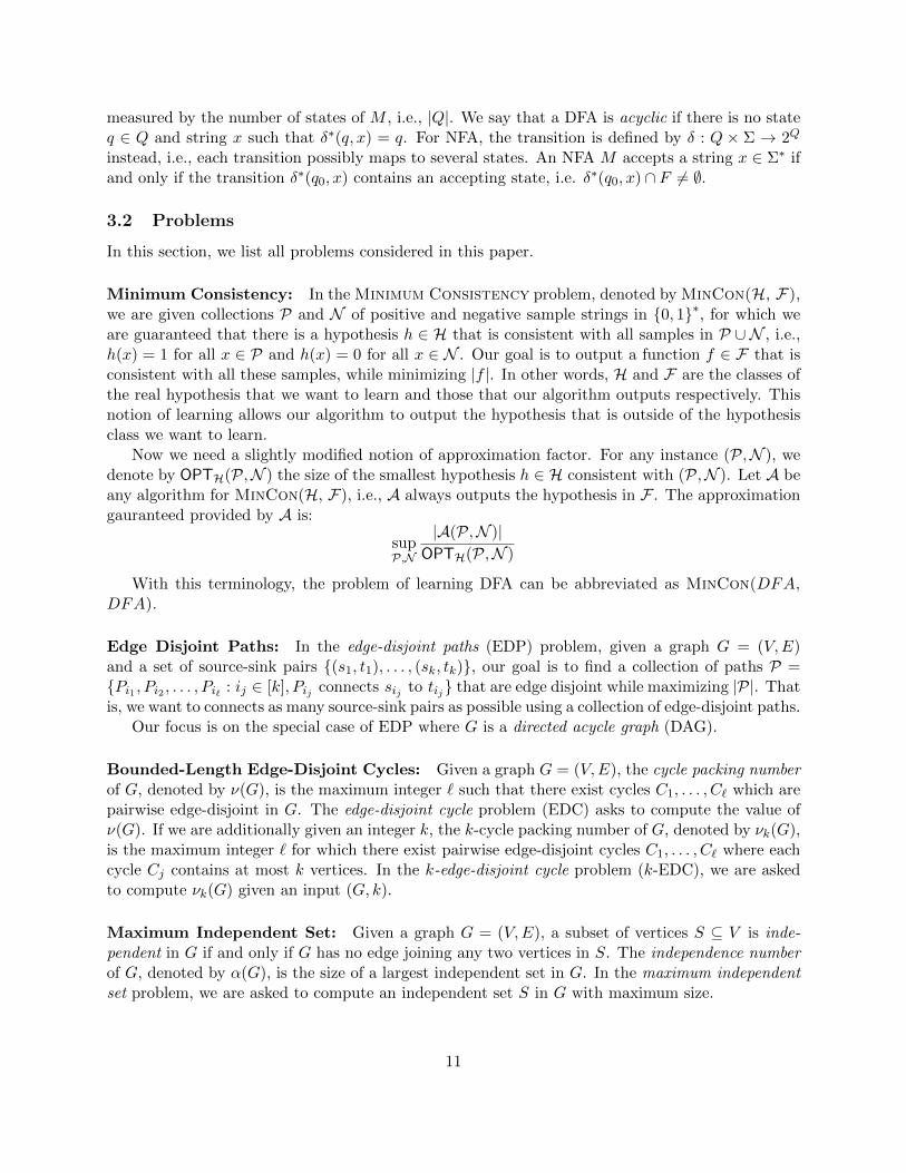
Minimum Consistency: In the Minimum Consistency problem, denoted by MinCon(H, F),we are given collections P and N of positive and negative sample strings in 0, 1∗, for which weare guaranteed that there is a hypothesis h ∈ H that is consistent with all samples in P ∪ N , i.e.,h(x) = 1 for all x ∈ P and h(x) = 0 for all x ∈ N . Our goal is to output a function f ∈ F that isconsistent with all these samples, while minimizing |f |. In other words, H and F are the classes ofthe real hypothesis that we want to learn and those that our algorithm outputs respectively. Thisnotion of learning allows our algorithm to output the hypothesis that is outside of the hypothesisclass we want to learn.

Now we need a slightly modified notion of approximation factor. For any instance (P,N ), wedenote by OPTH(P,N ) the size of the smallest hypothesis h ∈ H consistent with (P,N ). Let A beany algorithm for MinCon(H, F), i.e., A always outputs the hypothesis in F . The approximationgauranteed provided by A is:

supP,N

|A(P,N )|OPTH(P,N )

With this terminology, the problem of learning DFA can be abbreviated as MinCon(DFA,DFA).

Edge Disjoint Paths: In the edge-disjoint paths (EDP) problem, given a graph G = (V,E)and a set of source-sink pairs (s1, t1), . . . , (sk, tk), our goal is to find a collection of paths P =Pi1 , Pi2 , . . . , Pi` : ij ∈ [k], Pij connects sij to tij that are edge disjoint while maximizing |P|. Thatis, we want to connects as many source-sink pairs as possible using a collection of edge-disjoint paths.

Our focus is on the special case of EDP where G is a directed acycle graph (DAG).

Bounded-Length Edge-Disjoint Cycles: Given a graph G = (V,E), the cycle packing numberof G, denoted by ν(G), is the maximum integer ` such that there exist cycles C1, . . . , C` which arepairwise edge-disjoint in G. The edge-disjoint cycle problem (EDC) asks to compute the value ofν(G). If we are additionally given an integer k, the k-cycle packing number of G, denoted by νk(G),is the maximum integer ` for which there exist pairwise edge-disjoint cycles C1, . . . , C` where eachcycle Cj contains at most k vertices. In the k-edge-disjoint cycle problem (k-EDC), we are askedto compute νk(G) given an input (G, k).

Maximum Independent Set: Given a graph G = (V,E), a subset of vertices S ⊆ V is inde-pendent in G if and only if G has no edge joining any two vertices in S. The independence numberof G, denoted by α(G), is the size of a largest independent set in G. In the maximum independentset problem, we are asked to compute an independent set S in G with maximum size.

11

The following is the hardness results of the maximum independent set problem by Hastad6,which will be used to obtain the hardness of EDP on DAGs.

Theorem 3.2 ([Has96]+[Zuc07]). Let ε > 0 be any constant. Given graph G = (V,E), it isNP-hard to distinguish between the following two cases:

• (Yes-Instance:) α(G) ≤ |V (G)|ε

• (No-Instance:) α(G) ≥ |V (G)|1−ε

Chromatic Number: Given a graph G = (V,E), a proper coloring σ : V (G)→ [c] is a functionthat assigns colors to vertices of G so that any two adjacent vertices receive different colors assignedby σ (i.e., uv ∈ E =⇒ σ(u) 6= σ(v)). The chromatic number of G, denoted by χ(G), is theminimum integer c such that a proper coloring σ : V (G) → [c] exists, i.e., G can be properlycolored by c colors. In the graph coloring problem, we are asked to compute a proper coloringσ : V (G)→ [c] while minimizing c. We will be using the following hardness of approximation resultby Feige and Kilian [FK98]6.

Theorem 3.3 ([FK98]+[Zuc07]). Let ε > 0 be any constant. Given graph G = (V,E), it is NP-hardto distinguish between the following two cases:

• (Yes-Instance:) χ(G) ≤ |V (G)|ε

• (No-Instance:) χ(G) ≥ |V (G)|1−ε

4 Meta Theorems

In this section, we prove general theorems that will be used in proving most hardness results in thispaper. These theorems give abstractions of the (graph product) properties one needs to prove inorder to obtain hardness of approximation results. Our techniques can be used to derive hardnessesfor both minimization and maximization problems. For the former, the reduction is from minimumcoloring, while the latter is obtained via a reduction from maximum independent set.

Let us start with maximization problems. Suppose we have an optimization problem Π such thatany instance I ∈ Π is associated with an optimal function OPTΠ(I). We consider a transformationR that maps any graph G into an instance R[G] of the problem Π. We say that a transformationR satisfies a low α-projection property with respect to a maximization problem Π if and only if thefollowing two conditions hold:

• (I) For any graph G = (V,E), OPTΠ(R[G]) ≥ α(G).

• (II) There are universal constants c1, c2 > 0 (independent of the choices of graphs) such that,for any two graphs G and H,

OPTΠ(R[G ·H]) ≤ |V (G)|c1 + α(G)c2OPTΠ(R[H]).

6 The hardness results of the maximum independent set problem [Has96] and the graph coloring problem [FK98]hold under the assumption NP 6= ZPP. The results were later derandomized by Zuckerman in [Zuc07] and thus holdunder the assumption P 6= NP.

12

• (III) There is a universal constant c0 > 0 such that

OPTΠ(R[G]) ≤ c0|R[G]|.

Intuitively, the transformation R with the low α-projection property tells us that there arerelationships between the optimal solution of the problem Π on R[G] and the independence numberof G. Instead of looking for a sophisticated construction of R, we focus on a “simple” transformationR that establishes a connection on one side, i.e., OPTΠ(R[G]) ≥ α(G), and the “growth” of OPTΠ

is “slow” with respect to graph products. Property (III) of the low α-projection property says thatthe optimal is at most linear in the size of the instance, which is the case for almost every naturalcombinatorial optimization problem.

Next, we turn our focus to a minimization problem. In this case, we relate the optimal solutionto the chromatic number of an input graph. Specifically, one can define the low χ-projection propertywith respect to a minimization problem Π as follows.

• (I) For any graph G = (V,E), OPTΠ(R[G]) ≥ χ(G).

• (II) There are universal constants c1, c2 > 0 (independent of the choices of graphs) such that,for any two graphs G and H, we have

OPTΠ(R[G ·H]) ≤ |V (G)|c1 + χ(G)c2OPTΠ(R[H]).

• (III) There is a universal constant c0 > 0 such that

OPTΠ(R[G]) ≤ c0|R[G]|.

We observe that the existence of such reductions is sufficient for establishing hardness of ap-proximation results, and the hardness factors achievable from the theorems depend on the size ofthe reduction.

Theorem 4.1 (Meta-Theorem for Maximization Problems). Let Π be a maximization problem forwhich there is a reduction R for Π that satisfies low α-projection property with |R[G]| = O(|V (G)|d).Then for any ε > 0, given an instance I of Π, it is NP-hard to distinguish between the followingtwo cases:

• (Yes-Instance:) OPTΠ(I) ≥ |I|1/d−ε

• (No-Instance:) OPTΠ(I) ≤ |I|ε

Theorem 4.2 (Meta-Theorem for Minimization Problems). Let Π be a minimization problem forwhich there is a reduction R for Π that satisfies low χ-projection property with |R[G]| = O(|V (G)|d),for some constant d ≥ 0. Then for any ε > 0, given an instance I of Π, it is NP-hard to distinguishbetween the following two cases:

• (Yes-Instance:) OPTΠ(I) ≤ |I|ε

• (No-Instance:) OPTΠ(I) ≥ |I|1/d−ε

13

4.1 Proof of Theorem 4.1 (Meta Theorem for Maximization Problems)

Consider a reduction R that transforms a graph G into an instance of Π that satisfies the low α-projection property. We analyze how the optimal value changes over `-fold lexicographic products.

Lemma 4.3. For any positive integer `, OPTΠ(R[G`]) ≤ `c0|V (G)|c1+d+1α(G)2c2`

Proof. This is proved by induction on a positive integer `. The base case ` = 1 holds becauseOPTΠ(R[G]) ≤ c0|R[G]| ≤ c0|V (G)|d. Assume that the induction hypothesis holds for any ` > 1,and consider OPTΠ(R[G`+1]). By writing G`+1 = G·G` and applying the low α-projection property,we have

OPTΠ(R[G`+1]) ≤ |V (G)|c1 + α(G)c2OPTΠ(R[G`])

Then, by applying induction hypothesis, we have

OPTΠ(R[G`+1]) ≤ |V (G)|c1 + α(G)c2(`c0|V (G)|c1+d+1α(G)2c2`

)≤ |V (G)|c1 + α(G)c2+2c2``c0|V (G)|c1+d+1

≤ (`+ 1)c0|V (G)|c1+d+1α(G)2c2(`+1)

We note that the exponent of the term α(G) depends on ` (the number of times the productis applied), while that of |V (G)| does not. Intuitively speaking, this is why the contribution of theterm |V (G)|c1 vanishes after taking graph products.

Hardness of Approximation. Now we prove the hardness of approximation result claimed inTheorem 4.1. Start from graph G as given by Theorem 3.2. Then construct an instance R[G`] with` = d1/εe. This results in the instance R[G`] of the problem Π of size N = |R[G`]| = O(|V (G)|`d).

In the Yes-Instance, we have

OPTΠ(R[G`]) ≥ α(G`) = α(G)` ≥ |V (G)|(1−ε)` = N1/d−O(ε).

In the No-Instance, we have

OPTΠ(R[G`]) ≤ O(|V (G)|d+c1+1α(G)2c2`).

Since α(G) ≤ |V (G)|ε in this case, we have

α(G)2c2` ≤ |V (G)|2c2 = |V (G)|O(1) = NO(ε).

This implies that OPTΠ(R[G`]) ≤ |V (G)|O(1)NO(ε) = NO(ε), and the gap between Yes-Instanceand No-Instance is N1/d−O(ε). This completes the proof.

4.2 Proof of Theorem 4.2 (Meta Theorem for Minimization Problems)

Similarly to the case of maximization problems, we can prove the following lemma by inductionon integers `. We shall skip the proof as it is the same as that of Lemma 4.3 except that α(G) isreplaced by χ(G).

Lemma 4.4. For any positive integer `, OPTΠ(R[G`]) ≤ `c0|V (G)|c1+d+1χ(G)2c2`.

14

Hardness of Approximation Take the instance R[G`] with ` = d1/εe.In the Yes-Instance, we have the following bound, which is slightly different from the case of

the maximization problem.

OPTΠ(R[G`]) ≥ χ(G`) ≥ (χf (G))` ≥ |V (G)|`(1−2ε) = N1/d−O(ε).

In the No-Instance, Lemma 4.4 gives OPTΠ(R[G`]) ≤ NO(ε). Thus, we have the desired gap,completing the proof.

4.3 Overview of Applications

Most of the reductions in this paper are direct applications of the above two meta theorems. Thatis, we design the following reductions.

• A reduction REDP for EDP such that |Redp[G]| = O(|V (G)|2) and satisfies α-projection prop-erty. This implies a tight n1/2−ε hardness of approximating EDP on DAGs.

• A reduction Rfa for MinCon such that |Rfa[G]| = O(|V (G)|2) and satisfies χ-projectionproperty. This gives n1/2−ε hardness of approximating MinCon(NFA,ADFA).

Notice that the reduction Rfa above is not tight. To obtain a tight result, we need |Rfa[G]| =O(|V (G)|), and it seems difficult to obtain such a reduction. We instead exploit the further structureof graph products and prove bounds of the form

χ(Gk) ≤ OPT(R′fa[Gk]) ≤ χ(G)O(k)|V (G)|O(1)

Now our reduction size is smaller, i.e., |R′fa[Gk]| = |V (G)|(1+o(1))k as opposed to |Rfa[Gk]| =

|V (G)|2k. Moreover, the reduction R′fa exploits the fact that the input graph is written as a k-foldproduct of graphs. This more restricted form of graph products allows us to prove tight hardness(and PAC impossibility result) of DFA and DNF/CNF Minimization.

5 Hardnesses of Finite Automata Problems: Minimum Consis-tency and Proper PAC Learning

We show in this section the hardness of the consistency problems for finite automata, as well asthe implications on impossibility results for PAC learning. We start our discussion by proving thehardness for MinCon(ADFA,NFA), which includes the minimum consistent NFA problem (Min-Con(NFA,NFA)) as a special case. Then we proceed to prove the tight hardness of approximatingMinCon(ADFA,DFA), which implies the tight hardness of approximating the minimum consistentDFA problem and also implies the impossibility result for proper PAC-learning DFA.

5.1 Hardness of MinCon(ADFA, NFA) via Graph Products

In this section, we show an N1/2−ε hardness for MinCon(ADFA,NFA). Formally, we prove thefollowing theorem.

15

Theorem 5.1. Let ε > 0 be any positive constant. Given two sets of positive and negative samplestrings P,N over alphabet Σ = 0, 1 with a total length of N bits, it is NP-hard to distinguish thefollowing two cases:

• There is an acyclic deterministic finite automata of size N ε that is consistent with all stringsin P ∪N .

• Any non-deterministic finite automata consistent with P∪N must have at least N1/2−ε states.

This is done by designing a reduction R[G] with χ-projection property and |R[G]| = O(|V (G)|2).Our proof in fact shows that the projection properties hold for both optimal DFA and NFA func-tions.

5.1.1 The Reduction R

We will be working with binary strings, i.e., the alphabet set Σ = 0, 1. Given a graph G = (V,E),we construct two sets P,N of positive and negative samples, which encode vertices and edges of thegraph. We assume w.l.o.g. that |V (G)| = 2k for some integer k. Therefore, each vertex u ∈ V (G)can be associated with a k-bit string 〈u〉 ∈ 0, 1k.

Now our reduction R[G] is defined as follows. The positive samples are given by

P =〈u〉1〈u〉R : u ∈ V (G)

and the negative samples are

N =〈u〉1〈v〉R : uv ∈ E(G)

We denote this instance of the consistency problem by an ordered pair (P,N ). Now we proceed toprove property (I), that any NFA consistent with (P,N ) must have at least χ(G) states.

Lemma 5.2. Let M = (Q,Σ, δ, q0, F ) be an NFA that is consistent with (P,N ). Then for anyvertex u ∈ V (G),

δ∗(q0, 〈u〉) 6⊆⋃

v:uv∈E(G)

δ∗(q0, 〈v〉).

Proof. Assume for contradiction that δ∗(q0, 〈u〉) ⊆⋃v:uv∈E(G) δ

∗(q0, 〈v〉). Since 〈u〉1〈u〉R is a posi-

tive sample, there is a state q ∈ δ∗(q0, 〈u〉) that leads to an accepting state (i.e., δ∗(q, 1〈u〉R)∩F 6= ∅).By the assumption, the state q also belongs to another set δ∗(q0, 〈v〉) for some v : uv ∈ E(G).

Now consider the string 〈v〉1〈u〉R, which is a negative sample because vu ∈ E(G). Since q ∈δ∗(q0, 〈v〉) and δ∗(q, 1〈u〉R)∩F 6= ∅, the string 〈v〉1〈u〉R must be accepted by M , a contradiction.

Lemma 5.2 implies in particular that, for each vertex u ∈ V (G), the set δ∗(q0, 〈u〉)\(⋃

v:uv∈E(G) δ∗(q0, 〈v〉)

)is not empty. Now denote by OPTDFA(R[G]) and OPTNFA(R[G]) the number of states in the min-imum DFA and NFA that are consistent with the samples R[G] = (P,N )G, respectively.

Corollary 5.3. Any NFA M that is consistent with (P,N )G must have at least χ(G) states.Therefore, OPTDFA(R[G]) ≥ OPTNFA(R[G]) ≥ χ(G) for all G.

Proof. For each state q ∈ Q, define a set Cq =u ∈ V (G) : q ∈ δ∗(q0, 〈u〉) \ (

⋃v:uv∈E(G) δ

∗(q0, 〈v〉)

.

It is easy to see that Cq is an independent set and thus form a proper color class of G. Lemma 5.2implies that each vertex u ∈ V (G) belongs to at least one class. So, Cqq∈Q gives a proper|Q|-coloring of G, implying that |Q| ≥ χ(G).

16

5.1.2 χ-Projection Property

We will consider a specific class of DFA M = (Q,Σ, δ, q0, F ), which we call canonical DFA. Specif-ically, we say that a DFA is canonical if it has the following properties.

• The state diagram has exactly ` layers for some `, and each path from q0 to any sink haslength exactly `.

• All accepting states are in the last layer.

Denote shortly by OPT(R[G]) the number of states in the minimum canonical DFA consistentwith R[G]. So we have that OPT(R[G]) ≥ OPTDFA(R[G]) ≥ OPTNFA(R[G]). The followinglemma gives the χ-projection property for OPT(·)

Lemma 5.4. OPT(R[G ·H]) ≤ χ(G)(OPT(R[H]) +O(|V (G)|))

To prove this lemma, we show how to construct, given a canonical DFA for R[H], a “compact”canonical DFA for R[G · H]. We note that one key idea here is to avoid exploiting the DFA forR[G] but instead tries to use the color classes of G in its optimal coloring to “compress” the DFAfor R[G ·H].

Proof. Let MH = (QH , 0, 1 , δH , qH , FH) be the minimum DFA for the instance R[H] whosenumber of states is s = OPT(R[H]) and has `H = 2h+1 layers for h = dlog |V (H)|e. Let C1, . . . , CBbe the color classes of G defined by the optimal coloring, so B = χ(G). Let f : V (G) → [B] bethe corresponding coloring function. We will also be using several copies of a directed completebinary tree with 2k leaves, where each leaf corresponds to a string in 0, 1k and is associated witha vertex in V (G). Call this directed binary tree Tk.

We will use MH and Tk to construct a new acyclic DFA M that have at most B(s+O(|V (G)|))states and exactly ` = 2(k + `H) + 1 layers. Now we proceed with the description of machine

M = (Q, 0, 1 , δ, q, F ). We start by taking a copy of directed tree Tk, and call this copy T(0)k . The

starting state q is defined to be the root of T(0)k . This is the first phase of the construction. Notice

that there are k layers in the first phase, so exactly k positions of any input string will be readafter this phase. Each state in the last layer is indexed by state(〈v〉) for each v ∈ V (G).

In the second phase, we take B copies of the machines MH where the jth copy, denoted by

M(j)H = (Q

(j)H , 0, 1, δ(j)

H , q(j)H , F

(j)H ), is associated with color class Cj defined earlier. For each

vertex v ∈ V (G), we connect the corresponding state state(〈v〉) in the last layer of Phase 1 to the

starting state q(f(v))H . This transition can be thought of as a “null” transition which can be removed

afterward, but keeping it this way would make the analysis simpler. Since each copy of MH has2`H + 1 layers, now our construction has exactly 2`H + k + 1 layers.

In the final phase, we first extend all rejecting states in M(j)H by a unified path until it reaches

layer 2(`H + k) + 1. This is a rejecting state rej0. Now, for each j = 1, . . . , B, we connect each

accepting state in the last layer of M(j)H to the root in the copy T

(j)k again by a “null” transition,

so we reach the desired number of layers now (notice that each root-to-leaf path has 2(k+ `H) + 1

states.) The states in the last layer of T(j)k are indexed by state(j, 〈v〉). The accepting states of M

are defined as F =⋃Bj=1

state(j, 〈u〉R) : u ∈ Cj

, and the rest of the states are defined as rejecting.

This completes our construction. See Figure 2 for illustration.

17

MH

accept reject

0 1

0 01 1

Tk

0 1

0 01 1

Tk

MHMHMH

0 1

0 01 1

Tk

0 1

0 01 1

Tk

0 1

0 01 1

Tk

accept reject accept reject accept reject

Figure 2: The illustration of the construction in the proof of Lemma 5.4.

The size of the construction is |V (G)|+Bs+O(|V (G)|B) = B(s+O(|V (G)|)). The next claimshows that the machine M is consistent with samples obtained from the product of G and H, whichthus finish the proof.

Claim 5.5. Given a machine MH that is consistent with samples R[H], the machine M constructedas above is consistent with samples R[G ·H].

Proof. First we check the positive sample. For each vertex (u, a) ∈ V (G · H), the correspondingstring 〈(u, a)〉1〈(u, a)〉R can be thought of as x = 〈u〉〈a〉1〈a〉R〈u〉R. After the first k transitions,

the machine M will stop at the state q(f(u))H . Then the substring 〈a〉1〈a〉R will lead to an accepting

state in F(f(u))H (since MH is consistent with samples in R[H]). Now, at the current state, we are at

the root of the tree T(f(u))k , and we are left with the substring 〈u〉R. Since u ∈ Cf(u), the substring

〈u〉R leads to an accepting state. This proves that the machine M always accepts positive samples.Next, consider a negative sample 〈(u, a)〉1〈(v, b)〉R generated by the edge (u, a)(v, b) ∈ E(G).

Again, this can be thought of as 〈u〉〈a〉1〈b〉R〈v〉R. There are two possible cases:

• If uv ∈ E(G), then the machine will enter M(f(u))H after reading the substring 〈u〉. Next,

the machine reads the substring 〈a〉1〈b〉R. If it manages to reach the third phase without

rejection (i.e., MH accepts 〈a〉1〈b〉R), then it will enter the tree T(f(u))k . Note that there is no

edge joining two vertices in Cf(u) because it is a color class. Thus, the substring 〈v〉 leads toa rejection because uv ∈ E(G) implies that v 6∈ Cf(u).

(Notice that the rejection does not depend on what happens inside MH .)

18

• If u = v and ab ∈ E(G), then after the first k transitions, the machine enters M(f(u))H with

the input string 〈a〉1〈b〉R for ab ∈ E(H). Since MH is consistent with samples in R[H], this

would lead to a rejection in M(f(u))H and therefore in M .

We will also need the base case condition as required by the low α-projection property.

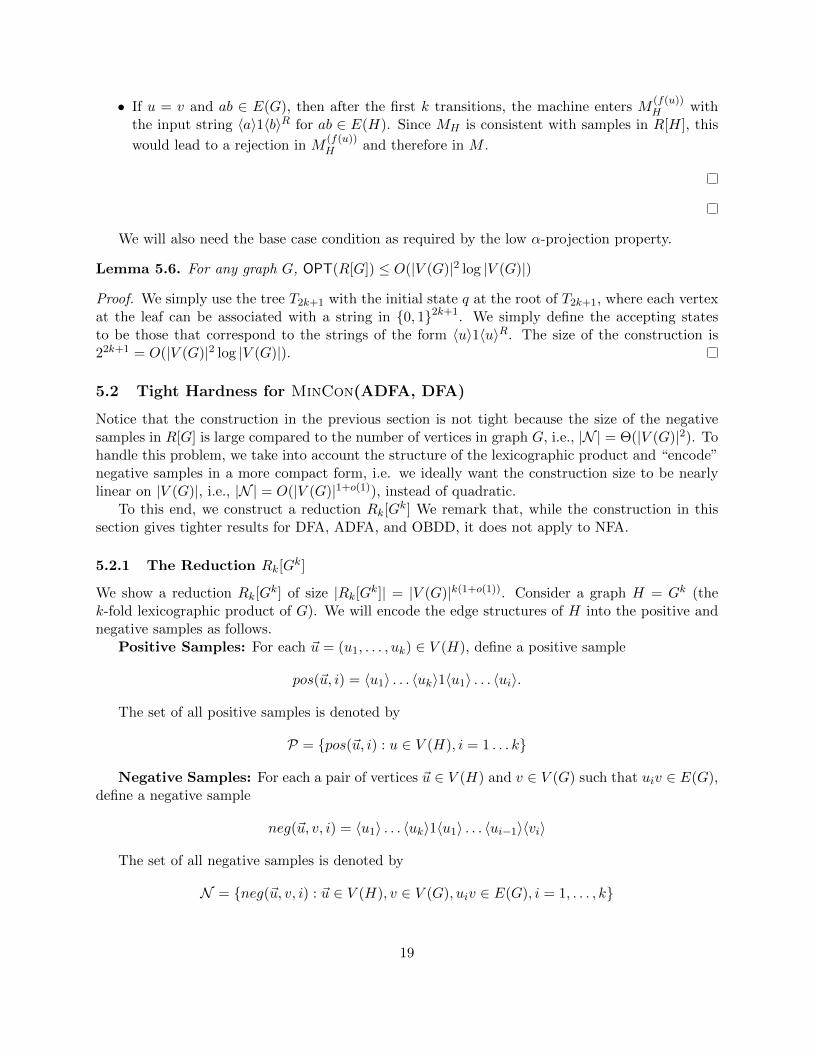
Lemma 5.6. For any graph G, OPT(R[G]) ≤ O(|V (G)|2 log |V (G)|)

Proof. We simply use the tree T2k+1 with the initial state q at the root of T2k+1, where each vertexat the leaf can be associated with a string in 0, 12k+1. We simply define the accepting statesto be those that correspond to the strings of the form 〈u〉1〈u〉R. The size of the construction is22k+1 = O(|V (G)|2 log |V (G)|).

5.2 Tight Hardness for MinCon(ADFA, DFA)

Notice that the construction in the previous section is not tight because the size of the negativesamples in R[G] is large compared to the number of vertices in graph G, i.e., |N | = Θ(|V (G)|2). Tohandle this problem, we take into account the structure of the lexicographic product and “encode”negative samples in a more compact form, i.e. we ideally want the construction size to be nearlylinear on |V (G)|, i.e., |N | = O(|V (G)|1+o(1)), instead of quadratic.

To this end, we construct a reduction Rk[Gk] We remark that, while the construction in this

section gives tighter results for DFA, ADFA, and OBDD, it does not apply to NFA.

5.2.1 The Reduction Rk[Gk]

We show a reduction Rk[Gk] of size |Rk[Gk]| = |V (G)|k(1+o(1)). Consider a graph H = Gk (the

k-fold lexicographic product of G). We will encode the edge structures of H into the positive andnegative samples as follows.

Positive Samples: For each ~u = (u1, . . . , uk) ∈ V (H), define a positive sample

pos(~u, i) = 〈u1〉 . . . 〈uk〉1〈u1〉 . . . 〈ui〉.

The set of all positive samples is denoted by

P = pos(~u, i) : u ∈ V (H), i = 1 . . . k

Negative Samples: For each a pair of vertices ~u ∈ V (H) and v ∈ V (G) such that uiv ∈ E(G),define a negative sample

neg(~u, v, i) = 〈u1〉 . . . 〈uk〉1〈u1〉 . . . 〈ui−1〉〈vi〉

The set of all negative samples is denoted by

N = neg(~u, v, i) : ~u ∈ V (H), v ∈ V (G), uiv ∈ E(G), i = 1, . . . , k

19

Intuitively, an edge in the the input graph represents a conflict between two vertices. Negativesamples are thus defined to capture a conflict (an edge) in the product of graphs between vertices~u and ~v at coordinate i. Notice that the size of positive and negative samples are |P| = knk and|N | = knk|E(G)| ≤ knk+2.

Let OPTADFA(·) denote the number of states in the optimal acyclic DFA that is consistent withthe samples. We will prove the following lemma.

Lemma 5.7. χ(H) ≤ OPTDFA(P,N ) ≤ OPTADFA(P,N ) ≤ χ(G)2k|V (G)|4.

The bound OPTDFA(P,N ) ≤ OPTADFA(P,N ) is trivial. For the other bounds, we will provethe left and right-hand side inequalities of Lemma 5.7 in Section 5.2.2 and Section 5.2.3, respectively.The hardness result then follows trivially from Theorem 3.3 and Theorem 3.1. In particular, takingthe hard instance of the graph coloring problem as in Theorem 3.3, we have that

Yes-Instance: OPTDFA(P,N ) ≤ χ(G)2kn4 ≤ nO(1).

No-Instance: OPTDFA(P,N ) ≥ χ(H) ≥ χ(G)k−o(1) ≥ n(k−O(1)).

Since |P|+ |N | = O(knk+2), this implies the hardness gap of (|P|+ |N |)1−ε, for any ε > 0.

5.2.2 The Lower Bound of OPTDFA

First, we show the lower bound for OPTDFA(P,N ). Let M = (Q,Σ, δ, q0, F ) be a DFA consistentwith (P,N ). We construct from M a |Q|-coloring of H: For each state q ∈ Q, we define a colorclass Cq = ~u : δ∗(q0, 〈~u〉) = q. Since M is deterministic, each vertex must get at least one color.

Lemma 5.8. For any vertices ~u,~v ∈ Cq, ~u~v 6∈ E(H). That is, Cq is a proper color class of H.

Proof. Suppose to a contrary that there is a pair of vertices~u,~v ∈ Cq such that ~u~v ∈ E(H). SinceH is obtained by the lexicographic product, there exists a coordinate i in which ~u and ~v conflict,i.e., uj = vj for all j < i and uivi ∈ E(G). We know that δ∗(q, 1〈u1〉 . . . 〈ui〉) ∈ F becausepos(~u, i) = 〈~u〉1〈u1〉 . . . 〈ui〉 is a positive sample. Since δ∗(q0, 〈~u〉) = δ∗(q0, 〈~v〉) = q, we mustalso have δ∗(q0, 〈v〉1〈u1〉 . . . 〈ui〉) = δ∗(q, 1〈u1〉 . . . 〈ui〉) ∈ F . But, this contradicts the fact thatneg(~v, ~u, i) = 〈~v〉1〈v1〉 . . . 〈vi−1〉〈ui〉 = 〈~v〉1〈u1〉 . . . 〈ui〉 is a negative sample.

5.2.3 The Upper bound of OPTADFA

Now we need to argue that there is an acyclic DFA M of size χ(G)2kn4. Suppose V (G) = 0, 1`.Let c = χ(G), and σ : V (G) → [c] be an optimal coloring of G. Our construction has two steps.First, we construct a complete rooted c-ary tree with 2k level, namely S. Note that S is a directedtree whose edges are oriented toward leaves. Each vertex in S except the root is associated withone color class from σ. In particular, for each internal vertex a of S, each child x of a is associatedwith a distinct color from [c]. We define the coloring of S by ρ : V (S) → [c]. Second, we replaceeach vertex a of S by a complete binary tree T with n leaves; we denote this copy of T by Ta.Each leaf q of Ta is associated with a vertex u of G and thus has a color σ(u) assigned. (We abuseσ(q) = σ(u) to mean a color of q.) For any vertex x in S that is a child of a, we join every leaf qof Ta with color σ(q) = ρ(a) to the root r of Tx. The transition edge qr is a null transition unlessa is a vertex at level k in S; for the case that a is at level k, the transition edge qr is labeled “1”.(Note that a null transition edge qr means that we will merge q and r in the final construction. Itis easy to see that this results in a DFA (not NFA) because S is a tree.) It can be seen that the

20

0 1

0 01 1

0 1

0 01 1

0 1

0 01 1

0 1

0 01 1

T

0 1

0 01 1

Ty TzTx

Ta

S

accept acceptaccept

accept

Figure 3: The illustration of the construction in the proof of Lemma 5.7.

constructed directed graph has a single source vertex (i.e., a vertex with no incoming edges), whichwe define as a starting state q0.

To finish the construction, we define accepting states. Let a0 be the root of S. Consider a vertexai at level i > k in S and its corresponding tree Tai . Since S is a tree, there is a unique path froma1 to ai, namely, P = a0, . . . , ak, ak+1 . . . , ai. For each leaf q of Tai , we define q as an acceptingstate if and only if σ(q) = ρ(ai−k+1), i.e., q and ai−k+1 receive the same color. See Figure 3 forillustration.

Each copy of T has at most 2n vertices, and S has at most c2k vertices. Thus, the size of theDFA M is at most 2nc2k. Also, observe that M is acyclic.

Lemma 5.9. The DFA M is consistent with (P,N ).

Proof. Consider any sample ~u ∈ P ∪N , which must be of the form:

~u = 〈u1〉 . . . 〈uk〉1〈uk+1〉 . . . 〈uk+i〉 for i : 1 ≤ i ≤ k and uj ∈ V (S) for all j = 1, . . . , k + i.

Note that uj = uk+j for all j = 1, 2, . . . , i − 1. The transition δ∗(q0, ~u) forms a path P inM , which traverses from the starting state q0 to some state qj . (That is, qj = δ∗(q0, ~u).) Byconstruction, P corresponds to the path a1, . . . , ai in S and thus must visit a leaf qj of tree Taj , forj = 1, . . . , i. Moreover, each qj is associated with vertex uj ∈ V (G). Notice that ρ(aj) = σ(uj−1)because we have an edge from qj−1 to Taj if and only if qj−1 and aj receive the same color.

21

If ~u is a positive sample in P, then we have ui−k = ui. (Note that qj and uj receive the samecolor for all j = 1, 2, . . . , k.) Since ai−k+1 has the same color as qi−k (and so does ui−k = ui), wehave ρ(ai−k+1) = σ(qi). Thus, qi is an accepting state.

If ~u is a negative sample in N , then we must have an edge ui−kui ∈ E(G). So, ui−k and uireceive different colors. Since ρ(ai−k+1) = σ(ui−k), it follows that ρ(ai−k+1) 6= σ(qi). Thus, qi is notan accepting state. This proves that M is consistent with both positive and negative samples.

5.3 Hardness of Proper PAC-Learning

Here we show that DFAs are not PAC-learnable. That is, we prove Corollary 1.2. We will use theconnection between PAC learning and the existence of an Occam algorithm, defined as follows.

Definition 5.10. An Occam algorithm for a hypothesis class H in terms of function classes Fis an algorithm A that for some constant k ≥ 0 and α < 1, the following guarantee holds. Leth ∈ H has size n and represents some language L(h). Then on any input of s samples of L(r),each of length at most m, the algorithm A outputs an element h ∈ H of size at most nkmksα thatis consistent with each of the s samples.

Therefore, an Occam algorithm for DFA is the case when H = DFA = F , and the measure ofthe size of each hypothesis h ∈ DFA is the number of states. It is known that PAC learnability ofDFA implies the existence of an Occam algorithm for the same hypothesis class as stated formallyin the following theorem.

Theorem 5.11 ([BP92], statement from [Pit89]). If DFAs are properly PAC-learnable, then thereexists a randomized Occam algorithm for DFA that runs in polynomial time.

Theorem 5.11 implies that, to prove Corollary 1.2, it suffices to rule out the existence of arandomized Occam algorithm for DFA, which is shown in the next Theorem.

Theorem 5.12. Unless NP = RP, there is no polynomial time randomized Occam algorithm forDFA.

Proof. We prove by contrapositive. Assume that there is a randomized Occam algorithm A forDFA with parameters (k, α) for some constants k ≥ 0 and 0 ≤ α < 1. Then we argue that therewould exist and an algorithm that distinguishes between the Yes-Instance and No-Instancegiven in Theorem 1.1. To see this, take an instance of MinCon(ADFA,DFA) as in Theorem 1.1.So, we have a pair of sets (P,N) of N samples, each of length O(logN). The parameters of theOccam algorithm A are thus s = N and m = O(logN).

We choose the parameter ε in Theorem 1.1 to be ε = (1− α)/(2k + 1).In the Yes-Instance, there is a DFA of size N ε consistent with the samples. Thus, our

hypothesis class has size n = N ε. By definition, the Occam algorithm A gives us a DFA M of size

|M | ≤ N εk · (logN)k ·Nα ≤ Nα+(2k)ε ≤ Nα+(2k) 1−α2k+1 = N1− 1−α

2k+1 = N1−ε

In the No-Instance, any DFA M consistent with (P,N) has size |M | > N1−ε.Therefore, the randomized Occam algorithm A can distinguish between the Yes-Instance and

No-Instance in Theorem 1.1, implying that NP = RP. This completes the proof.

A similar but weaker theorem can be proven for the case of NFAs. Indeed, we rule out theexistence Occam algorithm for NFA with parameter 0 ≤ α ≤ 1/2, assuming that NP 6= RP.

22

Theorem 5.13. Unless NP = RP, there is no polynomial time randomized Occam algorithm forNFA with parameter 0 ≤ α ≤ 1/2.

Proof. The proof is essentially the same as that of Theorem 5.12 with slightly different parameters.We prove by contrapositive. Assume that there is a randomized Occam algorithm A for NFA

with parameters (k, α) for some constants k ≥ 0 and 0 ≤ α ≤ 1/2. We will show that the algorithmA can be used to distinguishes between the Yes-Instance and No-Instance given in Theorem 1.4and thus implying that NP = RP .

Take an instance of MinCon(ADFA,NFA) as in Theorem 1.1. So, we have a pair of sets (P,N)of N samples, each of length O(logN). The parameters of the Occam algorithm A are thus s = Nand m = O(logN).

We choose the parameter ε in Theorem 1.1 to be ε = (1/2− α)/(2k + 1).In the Yes-Instance, there is an NFA of size N ε consistent with the samples. Thus, our

hypothesis class has size n = N ε. By definition, the Occam algorithm A gives us a NFA M withsize

|M | ≤ N εk · (logN)k ·Nα ≤ Nα+(2k)ε = Nα+(2k)1/2−α2k+1 = N1/2− 1/2−α

2k+1 = N1/2−ε

In the No-Instance, any NFA M consistent with (P,N) has size |M | > N1/2−ε.Therefore, the randomized Occam algorithm A can distinguish between the Yes-Instance and

No-Instance in Theorem 1.4, implying that NP = RP. This completes the proof.

Corollary 5.14. Unless NP = RP , there are no Occam algorithms for the following hypothesisclasses:

• Deterministic Finite Automata (DFA)

• Acyclic Deterministic Finite Automata (ADFA)

• Ordered Branching Decision Diagram (OBDD)

In particular, for any ε ∈ (0, 1), k > 0, the minimum consistent hypothesis problems for these classesare N1−εOPTk-hard to approximate unless NP = RP .

6 Hardness of EDP on DAGs

In this section, we prove the |V (G)|1/2−ε hardness of approximating EDP on DAGs and packingvertex-disjoint bounded length cycles. We will first show the construction for EDP, and later weargue that a slight modification of the construction yields the hardness of packing vertex-disjointbounded length cycles.

6.1 Reduction R

We first define the canonical reduction−→R [G] formally. Given a graph G = (V,E) on n vertices, the

switching graph of G, denoted by−→R [G], is a graph defined on a plane and constructed in two steps

as follows. The coordinates of graph−→R [G] lie in the box formed by the corners (0, 0) and (n, n).

First Step: For each vertex i ∈ V (G), we draw a line segment `i on the plane connectingvertices si and ti as shown in Figure 4. To be precise, the line `i goes from the coordinate (n+1−i, 0)

23

to the coordinate (n + 1 − i, i) of the grid and then goes to the coordinate (0, i). For each pairof vertices i, j ∈ V (G), we have an intersection point yi,j at the crossing point of lines `i and `j .Some of these intersection points will be later defined as vertices in the switching graphs whereasothers are just a crossing points in the plane embedding. We call this graph R[G] which will alsobe crucial in our analysis. Edges in R[G] are directed from left to right and top to bottom.

Second Step: For each edge ij ∈ E(G), we split yi,j into two vertices xini,j and xout

i,j and have

a directed edge ei,j = xini,jx

outi,j in the graph

−→R [G]. Otherwise, if ij 6∈ E(G), the intersection point

yi,j is replaced by an uncrossing as in Figure 4.

s(3)

t(4)

x(3,4)

x’(3,4)

x’’(3,4)

Figure 4: The graph−→R [G] where (3, 4) ∈ E(G) but (4, 5) 6∈ E(G)

First, the following lemma establishes a (simple) connection between EDP and the maximumindependent set problem.

Lemma 6.1. For any graph H, edp(−→R [H]) ≥ α(H).

Proof. Let S ⊆ V (H) be any independent set in H. We define the collection of paths PS = Pii∈Sin graph

−→R [H]. Since S is an independent set, any pair of paths Pi and Pj for i, j ∈ S are disjoint

by construction.

Unfortunately, the converse of this inequality does not hold within any reasonably small factor.

In fact, there is a graph H for which α(H) = 2 but edp(−→R [H]) = Ω(n); see Appendix A. Therefore,

we focus on proving the low α-projection property.

6.2 α-Projection Property

For technical reasons, we will need to analyze a slightly different measure from the optimal value

edp(−→R [G]). This notion will be a weaker notion of feasible solutions for EDP. We say that a

24

collection of disjoint paths P = P1, . . . , P` is orderly feasible if for any pair P = (si, . . . , tj)and P ′ = (si′ , . . . , tj′) such that i < i′, then it must be the case that j < j′; for instance, in anorderly feasible set, if we connect s1 to t3, it must be the case that s2 is connected to tj for j > 3.Intuitively, in an orderly feasible set P, a path is allowed to start from si and ends at some sinktj for j 6= i, but every pair of paths in P is forced to “cross” at some point. Observe that anycollection of feasible edge disjoint paths must also be orderly feasible. As a consequence, if we

define edp(−→R [G]) as the maximum cardinality of all orderly feasible collections of paths, then we

have that edp(−→R [G]) ≥ edp(

−→R [G]).

The following observation is more or less obvious.

Observation 6.2. For any graph G, edp(−→R [G]) ≤ |

−→R [G]|

Next, the following lemma will finish the proof of the low α-projection property.

Lemma 6.3. For any two graphs G and H,

edp(−→R [G ·H]) ≤ 3|V (G)|2 + α(G)edp(

−→R [H])

We will spend the rest of this section to prove the lemma.

6.3 Geometry of Paths: Regions, switching boxes, and configurations

This section discusses the structure of the graph−→R [G · H] and a feasible solution for EDP in

−→R [G ·H]. We define some terminologies that will be needed in the analysis.

Ordering of Paths We need a notion of “ordering” of edge-disjoint paths with respect to certaincurve. We think of graph R[G] as being drawn on the plane with standard x and y coordinates.All sources and sinks are on y and x axes respectively.

For any collection of edge-disjoint paths P in−→R [G], one can naturally map these paths on the

graph R[G] and think of them as curves on the plane. A continuous curve C : [0, 1] → R2 is saidto be good if for all t < t′, point C(t) is dominated by point C(t′) in the plane and the curve Cdoes not go through any intersection point yi,j (informally, the curve is directed to the top andright). Let C be any good curve. The ordering C is defined on the set of paths P ′ intersecting Cas follows: Paths P ≺C P ′ if and only if C intersects P before it intersects P ′. Since C does notintersect point yi,j , either P ≺C P ′ or P ′ ≺C P .

Regions and Switching Boxes. In−→R [G · H], we have canonical paths Pia for i ∈ V (G) and

a ∈ V (H). For each i ∈ V (G), we define a region Ri on the plane that contains all paths P(i,a) fora ∈ [r]. For i, j ∈ V (G), the intersection between regions Ri and Rj is called a bounding box B(i, j)which contains |V (H)|2 virtual vertices of the form Y (i, a), (j, b) for a, b ∈ V (H). Notice that acanonical path P(i,a) is completely contained inside region Ri, and as we walk on the path froms(i, a) to t(i, a), we will visit the bounding boxes B(i, 1), . . . , B(i, n) in this order. For convenience,the region in Ri between B(i, i− 1) and B(i, i+ 1) is called B(i, i). See Figure 6 for illustration.

Proposition 6.4. Consider any box B(i, j) for i 6= j. One of the following two cases holds:

• For all a, b ∈ V (H), the virtual vertex y(i,a),(j,b) is a directed edge e(i,a),(j,b). This happenswhen ij ∈ E(G), and we say that the box B(i, j) is a non-switching box.

25

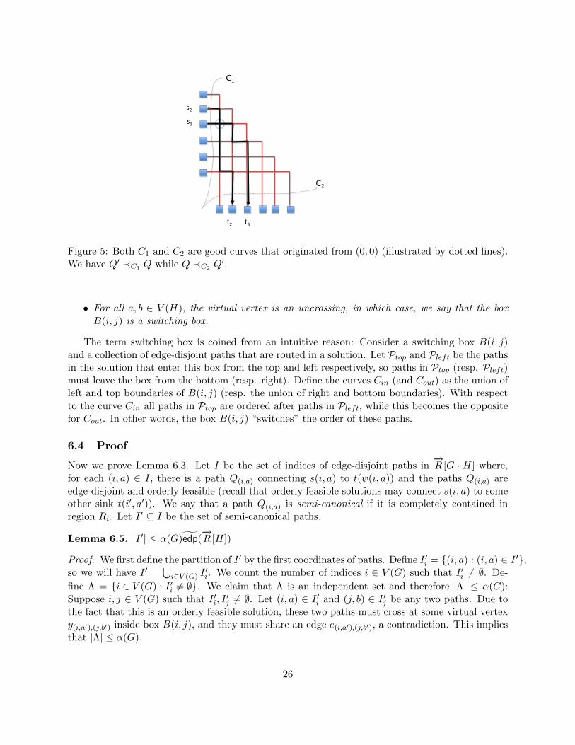
C1

C2

s3

s2

t2 t3

Figure 5: Both C1 and C2 are good curves that originated from (0, 0) (illustrated by dotted lines).We have Q′ ≺C1 Q while Q ≺C2 Q

′.

• For all a, b ∈ V (H), the virtual vertex is an uncrossing, in which case, we say that the boxB(i, j) is a switching box.

The term switching box is coined from an intuitive reason: Consider a switching box B(i, j)and a collection of edge-disjoint paths that are routed in a solution. Let Ptop and Pleft be the pathsin the solution that enter this box from the top and left respectively, so paths in Ptop (resp. Pleft)must leave the box from the bottom (resp. right). Define the curves Cin (and Cout) as the union ofleft and top boundaries of B(i, j) (resp. the union of right and bottom boundaries). With respectto the curve Cin all paths in Ptop are ordered after paths in Pleft, while this becomes the oppositefor Cout. In other words, the box B(i, j) “switches” the order of these paths.

6.4 Proof

Now we prove Lemma 6.3. Let I be the set of indices of edge-disjoint paths in−→R [G · H] where,

for each (i, a) ∈ I, there is a path Q(i,a) connecting s(i, a) to t(ψ(i, a)) and the paths Q(i,a) areedge-disjoint and orderly feasible (recall that orderly feasible solutions may connect s(i, a) to someother sink t(i′, a′)). We say that a path Q(i,a) is semi-canonical if it is completely contained inregion Ri. Let I ′ ⊆ I be the set of semi-canonical paths.

Lemma 6.5. |I ′| ≤ α(G)edp(−→R [H])

Proof. We first define the partition of I ′ by the first coordinates of paths. Define I ′i = (i, a) : (i, a) ∈ I ′,so we will have I ′ =

⋃i∈V (G) I

′i. We count the number of indices i ∈ V (G) such that I ′i 6= ∅. De-

fine Λ = i ∈ V (G) : I ′i 6= ∅. We claim that Λ is an independent set and therefore |Λ| ≤ α(G):Suppose i, j ∈ V (G) such that I ′i, I

′j 6= ∅. Let (i, a) ∈ I ′i and (j, b) ∈ I ′j be any two paths. Due to

the fact that this is an orderly feasible solution, these two paths must cross at some virtual vertexy(i,a′),(j,b′) inside box B(i, j), and they must share an edge e(i,a′),(j,b′), a contradiction. This impliesthat |Λ| ≤ α(G).

26

B(2,3)'

R3'

Figure 6: Regions and switching boxes in ~R[G]. There are two paths routed inside region R2.

Next, we argue that |I ′i| ≤ edp(−→R [H]) for all i ∈ Λ, which will complete the proof of the lemma.

If we consider the box B(i, i), we see an isomorphic copy H ′ of graph−→R [H], in which each path

Q(i,a) corresponds to another pathQ′ϕ(a) that connects some “source” s′(ϕ(a)) to “sink” t′(ξ(a)). We

claim that the collection of paths Q′ϕ(a) is orderly feasible in the instance (H ′, (s′(a), t′(a)a∈V (H)):

Assume otherwise that some paths Q′ϕ(a) and Q′ϕ(b) do not cross inside H ′, so the paths Q(i,a) and

Q(i,b) must cross at some other box B(i, j) for i 6= j. If such box is a switching box, it is impossiblefor these two paths to cross because they must enter and leave the box from the same direction;otherwise, if box B(i, j) is not a switching box, it is also impossible for them to cross.

Let I ′′ = I \ I ′. For convenience, let us renumber I ′′ such that I ′′ = 1, . . . , t such that thesource of path 1 is above that of path 2 and so on. Now we will show that |I ′′| ≤ 3|E(G)| + 1.Our proof will rely on the notion of configurations. We first define the order of boxes B(i, j) fori > j such that B(2, 1) is the first box, which precedes B(3, 1) (the second box), and so on. Moreformally, the box B(i, j) precedes B(i′, j′) if and only if i < i′ or i = i′ and j < j′; in short, this issimply a lexicographic order of boxes. This defines a total order over boxes.

We define a number of good curves C1, . . . , Cz for z =(|V (G)|

2

), where the curve Ch is any good

curve such that (i) Ch(0) = (0, 0), (ii) Ch(1) = (xmax, ymax) and (iii) the first h− 1 boxes are aboveCh, while z − h + 1 curves are below it (notice that Ch partitions the region [0, n + 1] × [0, n + 1]into two parts, i.e. one above the curve and the other below it).

Observation 6.6. For each h = 1, . . . , z and path i ∈ I ′′, the curve Ch intersects path i ∈ I ′′.

Proof. This is just because any path in the orderly feasible solution starts from the region abovethe curve Ch, while it ends in the region below the curve.

For each h = 1, . . . , z, a curve Ch can be used to define a configuration σh = (x1, . . . , xt) ofpaths in I ′′ where xj ∈ I ′′ is the index of the jth path that intersects with the curve Ch(this orderis well-defined because the curve has directions). Notice that σ1 = (t, . . . , 1), and σz = (1, . . . , t).

27

The number of reversals of a configuration σh is the number of locations j such that σj > σj+1.Denote this number by rev(σh), so we have that rev(σ1) = t − 1, and rev(σz) = 0. Our proofproceeds by analyzing how the number of reversals changes over configurations σ1, . . . , σz. We willshow that, for any h, we have rev(σh)−rev(σh+1) ≤ 3, which implies that t−1 = rev(σ1)−rev(σz) =∑z−1

h=1(rev(σh)− rev(σh+1)) ≤ 3(z− 1); in other words, |I ′′| = t ≤ 3z ≤ 3|V (G)|2. So the last thingwe need to prove is the following lemma:

Lemma 6.7. For any h = 1, . . . , z − 1, we have rev(σh)− rev(σh+1) ≤ 3.

Proof. Let B(i, j) be the hth box and J ⊆ I ′′ be the indices of paths entering this box. If the boxB(i, j) is a non-switching box, then it must be the case that σh+1 = σhdue to the fact that pathscannot cross inside region B(i, j). This implies that rev(σh) = rev(σh+1) in this case.

Now we consider the other case when B(i, j) is a switching box. We write J = Jtop ∪ Jleftwhere Jtop (and Jleft) is the set of indices of paths entering box B(i, j) from the top (and leftrespective). It is clear that paths coming out of the bottom and right of the box are exactly Jtopand Jleft respectively. Notice that, while the curve Ch crosses Jtop after Jleft, the curve Ch+1

would cross paths in Jleft before those in Jtop. The configurations σh and σh+1 can be written asσh = σ′σleftσtopσ′′ and σh+1 = σ′σtopσleftσ′′ respectively. See Figure 7 for illustration.

B(i,j)'Ch'

Ch+1'

1'2'3'

4'

Figure 7: Configurations of curve Ch and Ch+1 are σh = (4, 2, 1, 3) and σh+1 = (2, 1, 4, 3) respec-tively. In this case, σtop = (2, 1) and σleft = (4). Box B(i, j) is a switching box.

7 Other Problems

In this section, we prove the hardness of k-Cycle Packing and DNF/CNF Minimization. As notedpreviously, our proof for CNF minimization is an alternative proof of Aleknovich et al. [ABF+08].

28

7.1 Hardness of k-Cycle Packing for Large k

We consider the problem of packing edge-disjoint k-cycles in which our goal is to pack as many

cycles of length at most k as possible. We only need to slightly change the reduction−→R [G] as used

in Section 6 in the following way: In the second step, for each pair i, j ∈ V (G), if ij ∈ E(G), we dothe same, but for ij 6∈ E(G) (including the case when i = j), we make two new vertices on each linebefore and after the jump (see Figure 8). Also, we have a back edge from ti to si for each i ∈ V (G).

s3

t4

y3,4

xin3,4

xout3,4

y3,4

Y4,5

y4,5

ain4,5 bin4,5

aout4,5

bout4,5 t3 Back edge

Figure 8: The graph−→R [G] where (3, 4) ∈ E(G) but (4, 5) 6∈ E(G). The differences between this

gadget and EDP gadget only lies in the new vertices aini,j , aouti,j , b

ini,j , b

outi,j

With this reduction, any “canonical” cycle between source si to sink ti (and taking back edge

to si) must have length exactly 2n+ 2, so we choose the value k = 2n+ 2. Let edc(−→R ′[G]) denote

the optimal value of k-cycle packing. We now establish the connection between the optimal value

of EDP solution in−→R [G] and the k-EDC solution in

−→R ′[G].

Notice that for any cycle that uses only one back edge, there is a corresponding path from some

si to ti. The number of these cycles corresponds exactly to EDP(−→R [G]), so we can write

EDP(−→R [G]) ≤ edc(

−→R ′[G]) ≤ EDP(

−→R [G]) + edc(

−→R ′[G])

where edc(−→R ′[G]) is the number of cycles that use more than one back edge. The following lemma

says that these cycles must be longer than k, i.e. edc(−→R ′[G]) = 0. In other words, this implies that

edc(−→R ′[G]) = EDP(

−→R [G]).

Lemma 7.1. Let C be a cycle in−→R ′[G] that uses more than one back edge. Then |C| > k.

Proof. Any cycle C must start at some si and ends at si. Let i = i0, i1, . . . , i` = i be the indices ofthe source-sink pairs visited in the cycle C, i.e. the cycle goes through si0 → ti1si1 → si2 → . . .→

29

ti`si` . Observe that a path that goes from sj to tj′ visit exactly (n−j+j′) vertices of the form yi,j ,because such path must go right j′ times and go down n− j times (in arbitrary order). Combiningthis with sj and tj′ , such path would visit 2(n− j + j′ + 1) vertices. Therefore, the total length ofthe cycle C is

`−1∑j=0

2(n− ij + ij+1 + 1) = 2`(n+ 1) + 2(i` − i0) = 2`(n+ 1)

So this cycle would have been longer than the threshold k if ` > 1.

7.2 Learning CNF Formula

We present an alternative proof for the hardness of properly learning CNF using our framework.Our reduction is quite similar to Alekhnovich et al.’s (see [ABF+08]), but our proof highlights therole of graph products in the proof (while their construction cannot be seen as a standard graphproduct in any way).

Let G be any graph. We think of a vertex u ∈ V (G) as an integer in 1, . . . , n. For each vertexu ∈ V (G), we define an encoding 〈u〉 = 0u−110n−u. For each edge uv ∈ V (G), the encoding of anedge uv has two 1s at the positions corresponding to u and v. Our reduction encodes the k-foldgraph product H = Gk into samples as follows. For each ~u = (u1, . . . , uk) ∈ V (H), we define anegative sample neg(~u) = 〈u1〉 . . . 〈uk〉. For each ~u ∈ E(H), i ∈ [k] and uiv ∈ E(G), we define apositive sample pos(~u, v, i) = 〈u1〉 . . . 〈ui−1〉〈uiv〉〈ui+1〉 . . . 〈uk〉.

Notice that the total number of variables is nk, where we think of them as k blocks; in each ofwhich, there are n variables. Denote by z(i, u) the variable in block i ∈ [k] that corresponds to avertex u ∈ V (G).

Lemma 7.2. OPT(R[H]) ≥ χ(H)

Proof. Suppose∧Mj=1Cj be a CNF formular that is consistent with all samples. We claim that the

number of clauses M is at least χ(H). For each ~u ∈ V (H), let σ(~u) be the index such that Cσ(~u)

evaluates to false on sample neg(~u); this clause must exist since this is a negative sample (if thereare many such indices for vertex ~u, we choose any arbitrary one). Now for each s ∈ [M ], we definethe set of vertices Qs ⊆ V (H) as Qs = ~u : σ(~u) = s.

Claim 7.3. Qs is an independent set for all s ∈ [M ].

Proof. Assume otherwise that some ~u~v ∈ E(H) such that ~u,~v ∈ Qs. Let i be the index such thatuj = vj for all j < i and uivi ∈ E(G). Let X,Y ⊆ [k] × V (G) be the subset of variable indices

that appear positively and negatively in clause Cs, so we can rewrite Cs =(∨

(j,u)∈X z(j, u))∨(∨

(j,u)∈Y z(j, u))

. Since Cs evaluates to false on both neg(~u) and neg(~v), we can neither have

variable z(i, ui) nor z(i, vi) in the clause Cs: Suppose otherwise that (i, ui) ∈ X or (i, ui) ∈ Y ,then either neg(~u) or neg(~v) would have evaluated to true on clause Cs (contradicting ~u ∈ Qs).Similarly, if (i, vi) ∈ X or (i, vi) ∈ Y , then either neg(~v) or neg(~u) would have been true in clauseCs.

In other words, (i, u), (i, v) 6∈ X ∪ Y . But notice that pos(~u, vi, i)(i′,u′) = neg(~u)(i′,u′) for all(i′, u′) 6∈ (i, ui), (i, vi), so Cs must evaluate to false on input pos(~u, vi, i), a contradiction.

30

We have just shown that Qss∈[M ] is a valid M -coloring for graph H, so we must have M ≥χ(H), as desired.

Next, we prove the upper bound.

Lemma 7.4. OPT(R[H]) ≤ χ(G)knO(1)

Proof. We construct the same formula as in Aleknovich et al. That is, let I1, . . . , IM be colorclasses of G and σ : V (G) → [M ] be the corresponding coloring function. Define the formulafi(z) = ∧Mc=1 ∨u6∈Ic z(i, u), for i = 1, 2, . . . , k, and define f(z) = ∨ki=1fi(z). This formula can beturned into a CNF of size at most χ(G)k|V (G)|O(1).

Claim 7.5. The formula f is consistent with all the samples.

Proof. Consider each negative sample neg(~u) for ~u = (u1, . . . , uk) ∈ V (H). For each i ∈ [k], noticethat fi(〈ui〉) evaluates to false because ∨u6∈Iσ(ui)〈ui〉u is false (since ui ∈ Iσ(ui) is the only bit of 〈ui〉that is “1”). This implies that ∨ki=1fi(neg(~u)) is false.

Now consider, for each ~u ∈ V (H), v : uiv ∈ E(G) and i ∈ [k], a positive sample pos(~u, v, i). Weclaim that fi(pos(~u, v, i)) is true, which causes f(pos(~u, v, i)) to be true: Assume to the contrarythat fi is false, so some term ∨w 6∈Ic〈uiv〉w is false for some c; notice that it can be false only if〈uiv〉w = 0 for all w 6∈ Ic; since we have 〈uiv〉ui = 〈uiv〉v = 1, it must be the case that both ui andv belong to Ic, contradicting the fact that Ic is a color class.

8 Conclusion and Open Problems

We have shown applications of pre-reduction graph product techniques in proving hardness ofapproximation. For some applications, such as EDP, proving α-projection property implies tighthardness, but for some others, we need a more careful reduction of the form R[G`] (taking intoaccount the fact that the input is an `-fold product of graphs).

There are many open problems on edge-disjoint paths. Most notably can one narrow down thegap of undirected EDP between O(

√n) upper bound and log1/2−ε n lower bound? For directed

EDP, there is still a (relatively large) gap in the case of low congestion routing, between theupper bound of n1/c [KS04] and the lower bound of n1/(3c+23) [CGKT07] if we allow routing withcongestion c. We believe that our techniques are likely to work there (in a much more sophisticatedmanner), and it would potentially close this gap. This would resolve an open question in Chuzhoyet al. [CGKT07].

Another interesting problem is the cycle packing problem. For this problem, the approximabilityis pretty much settled on undirected graphs with an upper bound of O(log1/2 n) and a lower boundof log1/2−ε n [FS11, KNS+07]. On directed graphs, there is still a large gap between n1/2 andΩ( logn

log logn). For k-cycle packing problem, it is interesting to see whether our technique gives k1−ε

hardness for small k.

Acknowledgement: We thank Julia Chuzhoy for suggesting the EDP reduction and for relateddiscussions when the first author was still at the University of Chicago.

31

References

[Aar08] Scott Aaronson. 6.080/6.089 Great Ideas in Theoretical Computer Sci-ence, Spring 2008, Lecture 21. MIT OpenCourseWare, 2008. Available athttp://stellar.mit.edu/S/course/6/sp08/6.080/courseMaterial/topics/

topic1/lectureNotes/lec21/lec21.pdf.

[ABF+08] Michael Alekhnovich, Mark Braverman, Vitaly Feldman, Adam R. Klivans, and ToniannPitassi. The complexity of properly learning simple concept classes. J. Comput. Syst.Sci., 74(1):16–34, 2008. Announced at FOCS 2004.

[ABX08] Benny Applebaum, Boaz Barak, and David Xiao. On basing lower-bounds for learningon worst-case assumptions. In FOCS, pages 211–220, 2008.

[ACG+10] Matthew Andrews, Julia Chuzhoy, Venkatesan Guruswami, Sanjeev Khanna, KunalTalwar, and Lisa Zhang. Inapproximability of edge-disjoint paths and low congestionrouting on undirected graphs. Combinatorica, 30(5):485–520, 2010.

[Ang78] Dana Angluin. On the complexity of minimum inference of regular sets. Informationand Control, 39(3):337–350, 1978.

[AZ06] Matthew Andrews and Lisa Zhang. Logarithmic hardness of the undirected edge-disjointpaths problem. J. ACM, 53(5):745–761, 2006. Also, in STOC’05.

[BP92] Raymond Board and Leonard Pitt. On the necessity of occam algorithms. TheoreticalComputer Science, 100(1):157 – 184, 1992.

[BS92] Piotr Berman and Georg Schnitger. On the complexity of approximating the indepen-dent set problem. Inf. Comput., 96(1):77–94, 1992. Also, in STACS’89.

[CGKT07] Julia Chuzhoy, Venkatesan Guruswami, Sanjeev Khanna, and Kunal Talwar. Hardnessof routing with congestion in directed graphs. In STOC, pages 165–178, 2007.

[Chu12] Julia Chuzhoy. Routing in undirected graphs with constant congestion. In STOC, pages855–874, 2012.

[CK07] Chandra Chekuri and Sanjeev Khanna. Edge-disjoint paths revisited. ACM Transac-tions on Algorithms, 3(4), 2007.

[CKS05] Chandra Chekuri, Sanjeev Khanna, and F. Bruce Shepherd. Multicommodity flow,well-linked terminals, and routing problems. In STOC, pages 183–192, 2005.

[CKS06] Chandra Chekuri, Sanjeev Khanna, and F. Bruce Shepherd. An O(√n) approximation

and integrality gap for disjoint paths and unsplittable flow. Theory of Computing,2(1):137–146, 2006.

[CKS09] Chandra Chekuri, Sanjeev Khanna, and F. Bruce Shepherd. Edge-disjoint paths inplanar graphs with constant congestion. SIAM J. Comput., 39(1):281–301, 2009.

[CL12] Julia Chuzhoy and Shi Li. A polylogarithmic approximation algorithm for edge-disjointpaths with congestion 2. In FOCS, pages 233–242, 2012.

32

[CLN13a] Parinya Chalermsook, Bundit Laekhanukit, and Danupon Nanongkai. Graph productsrevisited: Tight approximation hardness of induced matching, poset dimension andmore. In SODA, pages 1557–1576, 2013.

[CLN13b] Parinya Chalermsook, Bundit Laekhanukit, and Danupon Nanongkai. Independent set,induced matching, and pricing: Connections and tight (subexponential time) approxi-mation hardnesses. In FOCS, pages 370–379, 2013.

[CLN14] Parinya Chalermsook, Bundit Laekhanukit, and Danupon Nanongkai. Coloring graphpowers: Graph product bounds and hardness of approximation. In LATIN, pages 409–420, 2014.

[DlH10] Colin De la Higuera. Grammatical inference: learning automata and grammars. Cam-bridge University Press, 2010.

[DLSS14] Amit Daniely, Nati Linial, and Shai Shalev-Shwartz. From average case complexity toimproper learning complexity. In STOC, pages 441–448, 2014.

[Fei02] Uriel Feige. Relations between average case complexity and approximation complexity.In STOC, pages 534–543, 2002.

[Fel08] Vitaly Feldman. Hardness of proper learning. In Encyclopedia of Algorithms. Springer,2008.

[FK98] Uriel Feige and Joe Kilian. Zero knowledge and the chromatic number. J. Comput.Syst. Sci., 57(2):187–199, 1998. Also, in CCC 1996.

[FS11] Zachary Friggstad and Mohammad R. Salavatipour. Approximability of packing disjointcycles. Algorithmica, 60(2):395–400, 2011.

[GKR+03] Venkatesan Guruswami, Sanjeev Khanna, Rajmohan Rajaraman, F. Bruce Shepherd,and Mihalis Yannakakis. Near-optimal hardness results and approximation algorithmsfor edge-disjoint paths and related problems. J. Comput. Syst. Sci., 67(3):473–496,2003. Also, in STOC 1999.

[GL14] Venkatesan Guruswami and Euiwoong Lee. Inapproximability of feedback vertex set forbounded length cycles. Electronic Colloquium on Computational Complexity (ECCC),21:6, 2014.

[Gol78] E. Mark Gold. Complexity of automaton identification from given data. Informationand Control, 37(3):302–320, 1978.

[Has96] Johan Hastad. Clique is hard to approximate within n1−ε. In FOCS, pages 627–636,1996.

[KK10] Kenichi Kawarabayashi and Yusuke Kobayashi. The edge disjoint paths problem ineulerian graphs and 4-edge-connected graphs. In SODA, pages 345–353, 2010.

[Kle96] Jon Michael Kleinberg. Approximation algorithms for disjoint paths problems. PhDthesis, Citeseer, 1996.

33

[Kle05] Jon M. Kleinberg. An approximation algorithm for the disjoint paths problem in even-degree planar graphs. In FOCS, pages 627–636, 2005.

[KMR97] David R. Karger, Rajeev Motwani, and G. D. S. Ramkumar. On approximating thelongest path in a graph. Algorithmica, 18(1):82–98, 1997.

[KNS+07] Michael Krivelevich, Zeev Nutov, Mohammad R. Salavatipour, Jacques Yuster, andRaphael Yuster. Approximation algorithms and hardness results for cycle packing prob-lems. ACM Transactions on Algorithms, 3(4), 2007.

[KS04] Stavros G. Kolliopoulos and Clifford Stein. Approximating disjoint-path problems usingpacking integer programs. Math. Program., 99(1):63–87, 2004.

[KT98] Jon M. Kleinberg and Eva Tardos. Approximations for the disjoint paths problem inhigh-diameter planar networks. J. Comput. Syst. Sci., 57(1):61–73, 1998.

[KV94] Michael J. Kearns and Leslie G. Valiant. Cryptographic limitations on learning booleanformulae and finite automata. J. ACM, 41(1):67–95, 1994. Announced at STOC 1989.

[LV88] Ming Li and Umesh V. Vazirani. On the learnability of finite automata. In COLT,pages 359–370, 1988.

[Pit89] Leonard Pitt. Inductive inference, DFAs, and computational complexity. Springer, 1989.

[PV88] Leonard Pitt and Leslie G. Valiant. Computational limitations on learning from exam-ples. J. ACM, 35(4):965–984, 1988.

[PW93] Leonard Pitt and Manfred K. Warmuth. The minimum consistent DFA problem cannotbe approximated within any polynomial. J. ACM, 40(1):95–142, 1993. Announced atSTOC 1989.

[RS95] Neil Robertson and Paul D. Seymour. Graph minors .xiii. the disjoint paths problem.J. Comb. Theory, Ser. B, 63(1):65–110, 1995.

[VV04] Kasturi R. Varadarajan and Ganesh Venkataraman. Graph decomposition and a greedyalgorithm for edge-disjoint paths. In SODA, pages 379–380, 2004.

[Zuc07] David Zuckerman. Linear degree extractors and the inapproximability of max cliqueand chromatic number. Theory of Computing, 3(1):103–128, 2007. Also, in STOC 2006.

34

Appendix

A List of Bad Examples

In this section, we provide the evidences that all the reductions considered in this paper are neithertrivially “working” nor subadditive in the sense of our previous SODA paper [CLN13a]. Therefore,we will need the new conceptual ideas introduced in this paper.

A.1 Edge Disjoint Paths

We show a graph G in which α(G) = 2 but EDP(−→R [G]) = n/3. To ensure that G does not have an

independent set of size 3, we define graph G by defining a triangle-free graph H and let G = Kn\H.We consider a set of vertices V (G) = A∪B∪C, where |A| = 1, . . . , n/3 , B = n/3 + 1, . . . , 2n/3and C = 2n/3 + 1, . . . , n. Graph H only have edges between A and B in such a way that, forany i ∈ A and j ∈ B, we have ij ∈ E(H) if and only if i−j > n/3. It is obvious that H is bipartite,so if we define G = Kn \H, we have α(G) = 2.

A"

B"

C"

A’" B’" C’"

Figure 9: Bad Example for EDP reduction

Now we check that EDP(−→R [G]) = n/3. For each i ∈ [n], let Ei denote the set of edges on the

canonical path from si to ti in−→R [G]. For each i ∈ B, we define a path Pi that:

• Start at si and go straight until it meets with an edge in Ei−n/3, at which the path turnsdownward (the turning is possible because we have an edge i(i− n/3) ∈ E(G)).

• The path goes downward until it meets with an edge in En−i+n/3, at which the path turnsagain towards the right.

• Once path Pi meets with an edge in Ei again, it takes a turn downward and remains so untilit reaches ti.

Observation A.1. For any i, j ∈ B, Pi ∩ Pj = ∅.

35