1

Precise H 1S-nS in Boltzmann-Hund double well potential and Sommerfeld-

Dirac theories probe chiral behavior of atom H

G. Van Hooydonk, Ghent University, Faculty of Sciences, Ghent, Belgium

Abstract. We consider generic Boltzmann-Hund double well potential (DWP) theory and find that, for atom H, the Sommerfeld-Dirac equation in QED transforms in a DWP (Mexican hat curve) for chiral systems. With either theory, the few precise H 1S-nS terms available probe the chiral nature of atom H. Pacs: 03.65.Pm

I. Introduction

By comparing 1S-2S for H (e-p+) and for mirror H (e+p-) [1-2], theorists hope to understand CPT.

However, Sommerfeld-Dirac equation (SDE) [3] gives fluctuations of ±14 kHz [4], too large to

interpret H 1S-2S, precise to 47 Hz [5], while H remains problematic until H data are confronted

with double well potential (DWP) theory for chiral systems [6]. We now prove that SDE and

DWP theories are almost degenerate. With either theory for precise 1S-nS [5,7-11], we find a

Mexican hat curve with H- and H-states, which proves that atom H is chiral indeed [12-13].

II. Theory

II.1 Generic Boltzmann-Hund type DWP theory for chiral (quantum) systems

Fig. 1 shows that dimensionless DWP in x or y=1-x describes a generic Mexican hat curve [6,14]

Mx=(1-x2)2=1-2x2+x4=(2y-y2)2=4y2-4y3+y4=y2(2-y)2=4y2(1-½y)2 (1)

Achiral or (too) symmetric systems have one minimum. Chiral or less symmetric systems (1) have

two, one for a left-, another for a right-handed system, with a maximum in between. As soon as

simple Mx (1) is detected in the simplest spectrum of simplest atom H, this is also prototypical for

chiral behavior. This straightforward conclusion is tested below with precise H 1S-nS [5,7-11].

II.2 Boltzmann-Hund type Mexican hat curve as contained in SDE for H bound state QED

Mx (1) is hidden in SDE, the cornerstone of bound state QED [3]. In standard notation [3], SDE

E(n,j)=μc2[f(n, j)-1]; f(n,j)=(1/√{1+α2/[√((j+½)2-α2)+n-(j+½)]2} (2)

gives the spectrum of Dirac Hamiltonian for relativistic H. For nP, expansion to order α4 gives

-EnP=½μα2c2(1/n2+α2/n3–¾α2/n4)+h.o.=(RH/n2)[1+1/3α2 -1/3α2(1-1,5/n)2]+h.o. (3)

Since the parabolic part between square brackets is like (1), even SDE suggests chiral H behavior.

In fact, (2) gives (3) using zero 0=+1/3RHα2/n2-1/3RHα2/n2, pending h.o. Reduced difference

ΔEnP/(1/3RHα2)=(-[EnP+(RH/n2)(1+1/3α2)]/(1/3RHα2)=(1/n2)(1-1,5/n)2 (4)

is the H Mexican hat curve, as contained in SDE: a plot of (4) versus (3/n-1) gives Mx in Fig. 1.

For 2S½, expected to be degenerate with 2P½, (2) was disproved [15]. We show in Appendix A

that DWP and SDE are degenerate within parts in 1016 [5] and adapt (3) for EnS in Appendix B.

2

II.3 Boltzmann-Hund chiral DWP HnS theory and H Mexican hat curve

If achiral nP term in (3) is EanP=-RH(1+1/3α2)/n2, Ea

nS=-RH(1+a)/n2 is expected for nS. With nP-

symmetry broken by EcnP=+1/3α4(1-nc(P)/n)2/n2, H nS-symmetry breaking will follow

EcnS=+aRH(1-nc(S)/n)2/n2 (5)

i.e. Mexican hat curve (1) [13], where a is of order α4μc2 or α2RH. In DWP HnS theory

-EnS(DWP)=Ean-E

cn=(RH/n2){1+a[1-(1-nc/n)2]/n2}=RH/n2+2anc/n3-an2

c/n4 (6)

critical nc(S) depends solely on the ratio of terms in 1/n3 and 1/n4 in (5). With Lamb shifts [15],

nc(S)≠ nc(P). Left-right differences are small: achiral H behavior follows α2; chiral H behavior, its

fine structure, follows α4. Fitting observed H terms

TnS=ΔE=|EnS-E1S| (7)

with Boltzmann-Hund chiral DWP theory therefore rests on EnS and TnS equations

-EnS(DWP)=RH/n2+A/n3-½Anc/n4 cm-1 and TnS= E1S-RH/n2-A/n3+½Anc/n4 cm-1 (8)

-nEnS(DWP)=RH/n+A/n2-½Anc/n3 cm-1 and nTnS=nE1S- RH/n-A/n2+½Anc/n3 cm-1 (9)

RnS=-n2EnS(DWP)=RH+A/n-½Anc/n2 cm-1 and n2TnS=n2E1S-RH-A/n+½Anc/n2 cm-1 (10)

wherein zero term in (3) is invisible. R nS (10) and the Mexican hat curve in (5) were found earlier

[12,13] but not yet with precise TnS. Which relation (8)-(10) to use rests on the number of precise

TnS available: (8) needs 5 in 4th order 1/n, (9) 4 in 3d order. With just 3 precise terms (see Section

III), only (10) can give a mathematically exact fit for available data.

III. Precise H 1S-nS intervals available

Table 1 gives observed (I) and derived (II) intervals, uncertainties σ and differences d with recent

[16] and older QED [17] (see [18]). For 3S and 6S, only difference D is known. Only relation (10)

can give an exact fit for 2S, 4S and 8S. A prediction for 3S awaits its measurement [19]. SDE for

precise 2S, 4S and 8S is in Appendix B, whereas QED for HnS is discussed in Appendix C.

IV. Boltzmann-Hund (BH) chiral H theory and precise H nS levels

T2S, T4S and T8S with σ=0 can be fitted exactly with a parabola in 1/n but the result is not reliable

for the complete nS-series. However, it gives a provisional E1S value

-E1S≈29979245800.109678,744663… Hz (11)

the starting point for an extended analysis to order 1/n4. We distinguish between σ=0 and σ≠0.

IV.1 Case 1: all σ=0

(i) Using (11), DWP parabola (10) leads to running Rydberg differences

±ΔRnS=±[n2(-E1S-TnS)-RH]≈±[n2(TnS-109678,74)-109678,74]=±A(1/n-½/n2) cm-1 (12)

with a maximum or a minimum. Any -E1S=RH value in (12) reproduces exactly the 3 input data

but only one can also accurately reproduce term D for 3S and 6S, not used as input.

(ii) Calculating D for –E1S, close to (11), gives the best E1S-value (13) by interpolation. We get

3

-E1S=RH=109678,77174371161…cm-1 = 3288086857146820 Hz (13)

-ΔRnS=29979245800(4,368693379685/n2-5,55578213674/n+1,188083721092) Hz (14)

TnS=29979245800[(109678,77174+3,71161.10-6)(1-1/n2)+4,368693379685/n4

-5,55578213674/n3+1,188083721092/n2)] Hz (15)

Parabola (14) in Fig. 2 leads to TnS (15), in exact agreement with observation, see Table 2. Fig. 2

shows Bohr RH=–E1S (13), SDE R∞S=109677,583659991 cm-1 but, at nc(S)=1,572665476, also

Rharm=29979245800*109679,350018514 Hz (16)

the harmonic Rydberg Rharm [12]. These 3 H asymptotes lead to 3 possible Mexican hat curves, to

be distinguished in Section VI. Reminding [21] for redirecting problems with E1S, we see that

(a) although (13)-(15) use σ=0, they give T1S≠0;

(b) BH fitting with QED value -E1S=109678,771743070 cm-1 [16] removes most QED errors in

Table 1, leads to an (allowed) error of +9795 Hz for D but, just like (a), gives T1S≠0 and

(c) using T1S=0 gives E1S= 109678,77174687022 cm-1, which returns input terms exactly but gives

a difference for D of 48223 Hz, too large to be explained by uncertainties in input data.

Using four data points T1S(=0), T2S, T4S and T8S, gives a small third term in 1/n3 for ΔRnS, absent

in (14). The resulting, slightly distorted higher order parabola for RnS gives terms, obeying

T’nS=-0,0038146973/n5+4,3727722168/n4-5,5572814941/n3-109677,583427429/n2

-0,0000383854/n+109678,771742861 cm-1 (17)

These reproduce observed data exactly too. The perturbation by a small term in 1/n5 does not

disprove the essential information on left-right or chiral H behavior (see Section VI).

IV.2 Case 2: σ≠0

The uncertainty σ for 2S is ±47 Hz but ±10000 Hz for 4S and ±8600 Hz for 8S, about 200 times

larger than for 2S (see Table 1). Neglecting small σ for 2S, 4S and 8S uncertainties

4S/8S |-σ(4S) 0σ(4S) +σ(4S) ------------------------------------------------------------------------------- -σ(8S) |-10000/-8600 0/-8600 +10000/-8600 0σ(8S) |-10000/0 0/0 +10000/0 +σ(8S) |-10000/+8600 0/+8600 +10000/+8600

lead to 9 maximum uncertainty scenarios. Plotting TnS (15) versus terms with uncertainties,

redirected to 1S-2S, gives ±10 kHz for 4S/8S σ-distributions +/+;-/- but these reduce to 50 %

for 0/+;0/- and +/0;-/0 and to 10% for +/-.-/+, as shown in Fig. 3. Rounding uncertainties are

about ±100 Hz. Numerical results for intermediate uncertainty scenario 0/±, are in Table 3.

V. Results and Discussion

Table 2 gives the differences with observed terms in Table 1 for 5 methods A-F, ordered by

decreasing average difference for observed terms (I). Results with perturbed parabola (17) and

with Kelly data [17] are discussed below. Differences are given in Hz, mainly to illustrate the

analytical power in reach. Old and recent QED methods A and B compare well. DWP/QED

4

method C and independent relativistic SDE quantum defect method D are close to DWP theory

E of Section III. Columns B and D show the improvement in precision due to DWP fitting. For

reproducing observed terms, SDE/DWP methods C-F are superior to QED methods A-B.

Table 3 gives TnS with B, D and E for n up to 20. Fig. 4 illustrates TnS-differences between

method E and all 4 methods A-D. This shows that C, D and E differ in the same way from B,

similar to A, see Table 2. TnS-differences are within precision limits of Appendix A (within NIST

Rydberg uncertainties ±22000(1-1/n2) Hz [20], see Fig. A1. TnS uncertainties with method E, also

shown in Fig. 4, are generated by observed uncertainties, following Section IV.2. To be complete,

we included TnS differences between E and method F using the perturbed parabola in (17).

Digits for TnS in Table 3 merely indicate the accuracy attainable with DWP fitting, as used in E. If

a better precision than in Table 1 had been available, this would be reflected immediately in TnS

by the analysis of Section III. With 2 nS input terms uncertain by ~10 kHz, discussing differences

for TnS would be academic, if it were not for a maximum discrepancy of over 10 kHz [18] for 1S-

3S between C-E and B [16], as clearly visible in Fig. 4. The outcome of [19] for will therefore be

important for H theories, especially for chiral H theory.

VI. Hund-type DWP or Mexican hat curve for chiral atom H

All methods above give a Mexican hat curve for H: curves are either exactly like (1) or good first

order approximations thereof, even with QED, based on SDE.

VI.1 Boltzmann-Hund H Mexican hat curve, based on precise H nS-terms

The H DWP for all σ=0 derives from equation (15). Level energies enS=EnS/c

-enS=109678,771743712/n2-1,188083721/n2 +5,555782137/n3-4,36869338/n4 cm-1 (18)

show large achiral, too symmetric Bohr contribution α2/n2 or RH/n2. Bohr could not differentiate

between left- or right-handed hydrogen, Coulomb attraction being equal in H (e-p+) and H (e+p-).

The small chiral, less symmetric part, with 3 terms α4/n2, α4/n3 and α4/n4, is responsible for the H

fine structure. This is in line with the idea that small left-right differences are only visible when

zooming in on a chiral system. The analytical form of the DWP in (18) depends on how term

(R∞S-R1S)/n2≈1,188…/n2 cm-1 is treated, which refers to the 3 Rydbergs, shown in Fig. 2.

(a) Subtracting –E1S/n2 from (18) gives a first asymmetric H quartic Qa, equal to

Qa=-enS-t∞/n2=-1,188083721/n2 +5,555782137/n3-4,36869338/n4 cm-1 (19)

Since -E1S is used as reference, DWP (19) is the most natural, observed quartic for atom H.

(b) Subtracting R∞H/n2=109677,583659991/n2 cm-1 gives a 2nd asymmetric Qb, equal to

Qb=-enS-R∞H/n2=Qa+1,188…/n2=+5,555782137/n3-4,36869338/n4 cm-1 (20)

The two asymmetric DWP (a) and (b) only differ by term 1,188…/n2, following (18)-(20).

(c) Subtracting achiral part Rharm/n2 leads to a 3d but symmetric DWP. Coefficients in (18) give

b2=4,36869338 cm-1 (b=±2,090141952) (21)

5

2ab=5,555782137 cm-1, giving a/b=ab/b2=0,635863… or nc(S)=b/a=1,572665476 (22)

a2=(½5,555782137/√(4,368693379))2=1,766358523 cm-1 (a=±1,329044…) (23)

Adding a zero term, i.e. by adding and subtracting term a2/n2 (a particle-antiparticle term of order

μα4 or α2RH) does not alter energy spectrum (2): it gives equivalent enS and symmetric Qc, obeying

-enS=(Rharm/n2)[1-(1,766358523/Rharm)(1-1,572665476/n)2]

=109679,350018514/n2-1,766358523(1-1,572665476/n)2/n2 cm-1

Qc=-enS-RHarm/n2=-1,766358523(1-1,572665476/n)2/n2 cm-1 (24)

The 3 H DWPs (19), (20) and (24) are graphically presented in Fig. 5. To get at (1), we see that

critical nc(S)=b/a (22) for (a-b/n)2 becomes 2nc(S)=2b/a for (a-b/n)2/n2. A plot of Qc (24) versus

x=2nc(S)/n-1=2.1,572665476/n-1=3,145330952/n-1 (25)

shown in Fig. 6, reveals that this 3d harmonic, symmetric Qc transforms in

Q’c=0,044636093x4-0,089272185x2+0,044636093=0,044636093(1-x2)2 cm-1 (26)

equivalent with generic Mx (1) in Fig. 1. Dimensionless (26) returns Mx (1) exactly by virtue of

MH=Qc/0,044636093≡(1-x2)2 (27)

Result (27) finally and quantitatively validates our straightforward conclusion on chiral atom H in

Section II.1 as well as earlier conclusions [12-13]. Uncertainties in Table 1 affect the shape of MH

but slightly and their effect is invisible on the scale of Fig. 6 (0,05 cm-1).

VI.2 H Mexican hat curves from QED/SDE theories

In fact, H Mexican hat curves with methods A-E all coalesce to the black curve in Fig. 6. In

lower resolution, differences between them remain invisible. Even the H Mexican hat curve (red

dashes in Fig. 6), generated from much less precise Kelly data [17] in Appendix D, nearly

coincides with that for (26). The different nc(S) and Rharm values are collected in Table 4.

VII. Discussion

(i) Fig. 6 and Table 4 show that all data and H theories available invariantly probe H chiral. With

BH theory, chiral H results are self-explanatory and straightforward. Energies EnS in the 2 wells

of chiral H reveal that n-values between ∞ and 2nc(S) apply for left-handed H-states (Bohr states)

with bound e-p+ pair at longer range, whereas those between 2nc(S) and 1 gives right-handed H-

states for bound e+p- pair at shorter range (or vice versa). The H e-p+ pair is confined to long

range (macroscopic level, H dissociation), in line with Bohr theory. The bound short-range e+p-

pair in H contradicts the long-range process in [1-2], see [22]. It is impossible to explain this H

phase transition by n, ℓ, spin ±½, since these remain constant throughout series nS, nP….

(ii) Chiral atom H does not contradict SDE, since this is nearly degenerate with BH closed form

theory (see Appendix A). BH theory leads to conceptual and computational advantages for

interpreting H fine structure, including a simple approach to the barrier height in the H DWP.

6

(iii) H 1S-3S, not used as input, should be available with a precision better than 1 kHz [19] to test

of chiral H. It would be a better 4th reference point but only if less uncertain than term D, used in

Section III. This also calls for a better precision for term D itself. The ideal case would be if

much more TnS terms were available as precisely as possible (T3S-data in Table 3 are in bold).

(iv) A test of whether or not T1S=0 is also needed, reminding problems on redirecting E1S [21], as

shown also in Table 3. If T1S≠0, as it seems here, calibration problems may emerge. With the few

precise terms now available, T1S=0 would require higher order contributions as in (17). Although

important, calibration-issues are beyond the scope of this work.

(v) The magnitude of the H fine structure is connected with the coefficient of term 1/n3. For nP,

this gives α2R∞H≈109677,583…/137,0362=5,84…but reduces to 5,55…. for nS. Their ratio gives

parameter b (B8) in Appendix B for the Sommerfeld quantum defect.

(vi) H DWPs contain potential difference (1-nc/n)2-1=-2nc/n+nc2/n2, i.e. a Kratzer potential [23].

Kratzer was a pupil of Sommerfeld, who already proposed SDE in 1916 [23]. The intimate

relation between a classical Mie-type potential like Kratzer’s and SDE now easily follows [24].

(vii) Critical nc(S) in (22) and Table 4 is either close to ½π [12,13] or to 2φ½= 1,572302756, where

φ=½(√5-1) is Euclid’s golden number [18]. With φ, Euclidean H coefficients

9φ½/4=1,768840600 and 2φ½=1,572302756 (31)

are close to those in (24). Euclidean H DWP (9φ½/4)(1-2φ½/n)2/n2 derives solely from H mass

mH=me+mP [18]. With φ, concentric circular orbits for nS would also point to spiral behavior (in

line with macroscopic cosmological evidence), if not to chaotic behavior [6,18].

(viii) With achiral, polarization independent terms 1/α2≈2.104 times larger than polarization-

dependent chiral terms, the latter will hardly be visible by variations in line intensities. The H

spectrum suggests polarization dependent wavelength shifts (PDWSs) [24b].

(viii) For the spectrum of relativistic H (2) to expose generic DWP (1), a zero correction is

needed, which seems a contradictio in terminis. In Section II.2, this zero for EnP is qualified as

0=+1/3RHα2/n2-1/3RHα2/n2=+(μα4c2/n2)6-(μα4c2/n2)6=+1,9468-1,9468 cm-1- (32)

This zero correction in 1/n2 may vanish in SDE (2) but it is essential to get at H Mexican hat

curve (1), see Section VI. Knowing symmetry is important for physics [25], this zero term plays

an important role, especially when looking at the simplicity of BH chiral DWP H theory.

(ix) Deciding on a person’s handedness is difficult when at rest, not perturbed…. Handedness

only shows upon performing tasks (eating, writing…). Deciding on H handedness is equally

difficult for only one state: it shows when perturbed, when in different fields hν. Unlike [1-2],

handedness of natural, neutral, composite system H shows through a n-series, see Fig. 1 and 6.

(x) It appears that, willingly or not, master SDE for bound systems (2), if not the Special Theory

of Relativity (STR) in (B11), describes natural left-right differences, following 19th century work

by Boltzmann, Pasteur, Le Bel and many others [6].

7

VIII. Conclusion

Chiral atom H [12,13,25] is given away in any resolution by any theory. SDE, proposed long

before spin [23,24], reveals a Boltzmann-Hund H DWP for its fine structure, due to chiral H

behavior. More data should reveal whether chiral H symmetry is continuous or discrete in the full

n-interval. A Mie-type Kratzer potential for atom H also appears in the potential energy curve

(PEC) for bond H2 [26]. As argued before [22,27], the precise generic H DWP found here puts

doubts on H-synthesis [1-2] and on common views on neutral matter-antimatter pairs.

References

[1] M. Amoretti et al., Nature 419 (2002) 456 [2] G. Gabrielse et al., Phys. Rev. Lett. 89 (2002) 213401’ [3] M.I. Eides, H. Grotch and V.A. Shelyuto, Phys. Rept. 342 (2001) 63; T. Kinoshita, Rep. Progr. Phys. 59 (1996) 1459 [4] G. Van Hooydonk, in preparation (see Appendix A of this paper) [5] M. Niering et al., Phys. Rev. Lett 84 (2000) 5496 [6] F. Hund, Z. Phys. 43 (1927) 806; see also H. Schachner, Ph.D. Thesis, U Regensburg, 2001; R.Weindl, Ph.D. Thesis, U Regensburg, 2002 (http://epub.uni-regensburg.de/9947). For a first DWP, see L. Boltzmann, Pogg. Ann. Phys. Chem., Jubelband (1874), 128 [7] M. Fischer et al., Phys. Rev. Lett. 92 (2004) 230802 [8] M. Fisher et al., Lect. Notes Phys., 648 (2004) 209 [9] B. de Beauvoir et al., Phys. Rev. Lett. 78 (1997) 440 [10] M. Weitz et al., Phys. Rev. A 52 (1995) 2664 [11] S. Bourzeix et al., Phys. Rev. Lett. 76 (1996) 384 [12] G. Van Hooydonk, Phys. Rev. A 66 (2002) 044103 (arxiv:physics/0501144) [13] G. Van Hooydonk, Acta Phys Hung NS 19 (2004) 385 (arxiv:physics/0501145) [14] J. Trost and K. Hornberger, Phys. Rev.Lett 103 (2009) 023202 [15] W.E. Lamb Jr. and R.C. Retherford, Phys. Rev. 72 (1947), 241. An immediate solution by H. A. Bethe, Phys. Rev 72 (1947), 339 led to Bethe-Salpeter theory (H.A. Bethe and E.E. Salpeter, Quantum Mechanics of One and Two Electron Atoms, Plenum, New York, 1977) [16] For recent NIST QED H TnS, see http://physics.nist.gov/PhysRefData/HDEL/index.html [17] G.W. Erickson, J. Phys. Chem. Ref. Data 6 (1977) 831(for older less precise TnS, see R.L. Kelly, J. Phys. Chem. Ref. Data 16 (1987) Suppl. 1) [18] G. Van Hooydonk, arxiv:0902.1096 [19] O. Arnoult et al., Can. J. Phys. 83 (2005) 273 [20] P.J. Mohr, B.B. Taylor and D.B. Newell, Rev. Mod. Phys. 80 (2008) 633 [21] J. Reader, Appl. Spectr. 58 (2004) 1469 [22] G. Van Hooydonk, physics/0502074 [23] A. Kratzer, Z. Phys. 3, (1920) 289; Ann. Phys. 67 (1922) 127 and references in [25]; A. Sommerfeld, Ann. Phys. (Berlin) 50 (1916) 1; La constitution de l’atome et les raies spectrales, 3d ed., Blanchard, Paris 1923 (1st ed., Atombau und Spektrallinien,Vieweg & Sohn, Braunschweig 1919). For a recent application of Kratzer’s potential, see O. Aydogdu and R. Sever, Ann. Phys. 325 (2010) 379 [24] a) L.C. Biedenharn, Found. Phys. 13 (1983) 13; b) G. Van Hooydonk, arxiv: physics/0612141 [25] D.J. Gross, Proc. Nat. Acad. Sci. USA 93 (1996) 14256. For H symmetry, see J.L. Chen, D.L. Deng and M.G. Hu, Phys. Rev. A 77 (2008) 034102 [26] G. Van Hooydonk, Z. Naturforsch. 64A (2009), 801 (arxiv:0806.0224); Eur. J. Inorg. Chem., Oct. (1999) 1617; Spectrochim. Acta A 56 (2000) 2273 (physics/0001059; 0003005); Phys. Rev. Lett. 100 (2008) 159301 (physics/0702087); G. Van Hooydonk and Y.P. Varshni, arxiv:0906.2905; [27] G. Van Hooydonk, Eur. Phys. J. D 32 (2005) 299 (physics/0506160);

8

Appendix A Precision of SDE and Boltzmann-Hund DWP The uncertainty for H 2S in Table 1 is 1,9.10-14. Last digit 3 in observed 2466061413187103(47)

Hz [7] is rounded to zero in double precision, giving an error of 1,2165.10-15. Double precision

10-16 for fnP times E0/h=μc2/h=[me/(1+me/mP)]c2/h=1,23491741822076.1020 Hz [20] gives

uncertainties of order 1,2.1020.10-16, larger than 10 kHz. Problems with double precision for fnP

can easily be quantified using the analytically exact transform f’nP in

fnP=1/√[1+α2/(n-γ)2]≡(1-γ/n)/√[1-2γ(1-1/n)/n]=f’nP (A1)

where Sommerfeld’s quantum defect γ for nP is

γ=1-√(1-α2)≈½α2+⅛α4+… (A2)

with 1/α=137,035999679 [20]. Whereas fnP/f’nP≡1 or fnP-f’nP≡0, differences between fnP-1 and

f’nP-1 are of order 10-16 in double precision. For n=1 to 300, EnP differences of ±13710 Hz in Fig.

A1, are in line with ±22000(1-1/n2) Hz for RN=3,289841960361(22).1015 Hz [20], also shown in

Fig. A1. Although double precision 10-16 is reasonable for physics experiments, master SDE is

unreliable for precise H data. Since it is uncertain which of fnP and f’nP is the better option, a

closed form quartic is preferable. If close to SDE, this avoids unwanted uncertainties. Fitting

SDE (2) in 1/n to 4th, 5th and 6th order, reveals that the best fit is 4th order (5th and 6th give much

larger discrepancies, not discussed here). As SDE h.o. start with α6/n6,

-EnP=½μα2c2(1/n2+α2/n3–¾α2/n4)+h.o.=½μα2c2[1/n2+(1+½α2)α2(1/n3–¾/n4] (A3)

gives a nP quartic, well within SDE fluctuation limits, as also illustrated in Fig. A1. A factor of

(1+½α2) for terms 1/n3 and 1/n4 amply suffices. Skipping this correction gives a difference of 1

MHz for n=1 but it is far from certain whether or not this correction is needed. Linear fits in Fig.

A1 reveal that (A3) is closer to f’nP than to fnP. For terms (7), fnP and f1P lead to

TnP=μc2{1/√[1+α2/(n-γ)2]-1/√[1+α2/(1-γ)2]}=μc2{1/√[1+(α2/n2)(1-γ/n)2]-√(1-α2)}(A4)

(for T’nP, f’nP and f’1P apply). Fluctuations for TnP can be twice as large as for EnP. We see that

(a) closed form (A3) describes in a continuous way (i.e. without fluctuations) the same quantum

systems, believed to obey original master SDE (2), the spectrum of the H Dirac Hamiltonian;

(b) for precise data, problems occur using fitting with fnP or f’nP with their inverse square root and

(c) an accurate low order fit with SDE variable B2nP=(α2/n2)(1-γ/n)2 would mean that adding

terms to the SDE expansion as in bound state QED [3] could be superfluous.

Appendix B Observed H 1S-nS and Sommerfeld’s quantum defect method

We elaborate on (b)-(c) in A. Using Sommerfeld’s quantum defect γP, EnP leads to

-EnP=μc2{1/√[1+(α2/n2)/(1-γ/n)2]-1}=μc2[1/√(1+B2nP)-1] (B1)

B2nP=(α2/n2)/(1-γ/n)2 (B2)

It is impossible to fit observed terms accurately with [1/√(1+B2nP)-1]: its physically meaningless

fluctuations are larger than experimental uncertainties, see point (b) above.

An expansion of (B1) in variable (B2) can be truncated to give

9

EnP=μc2(1-½B2nP+⅜B4

nP-… -1) (B3)

Without loss of accuracy, replacing unit 1 by 1/6 leads to a perfect parabola in B2nP, i.e.

EnP=μc2(1/6-½B2nP+⅜B4

nP-… -1/6)=μc2[(√6-1-√⅜.B2nP)

2…-6-1] (B4)

To apply this for TnS, variable (B2) must be parameterized. Without altering α, p would lead to γp

and variable BnS, as defined in γp=p-√(p2-α2). As p cancels in first order, we suffice by using b in

γp=1-√(1-bα2); B2nS=(α2/n2)/(1-γp/n)2 (B5)

With b close to 1, differences between nP and nS are quantified (Lamb shifts). EnS and TnS obey

EnS=μc2[(√6-1-√⅜.B2nS)

2…-6-1]

TnS=μc2[-½(B2nS-B

21S)+⅜(B4

nS-B41S)]= μc2{-½(B2

nS-B21S)[(1-¾(B2

nS+B21S)]} (B6)

(T1S=1/√(1+B2nS)-1/√(1+B2

1S)=0). To fit observed H 1S-nS terms in cm-1 with (B6) and to avoid

at the same time any the unwanted fluctuations of SDE, we use reduced squared variable

B’2nS=B2nS/α2=(1/n2)/(1-γp/n)2 (B7)

Since only 3 nS states are precisely known (σ=0), a 2nd order fit in (B7) is exact. This independent

relativistic SDE alternative avoids the procedure with running Rydbergs (10) as well as 4th order

fitting in 1/n for which 5 data points are needed. As in Section III, we redirect the 2nd order fit

for 3 observed nS terms to give exactly term D in Table 1 for non-input data on 3S and 6S. With

b=0,951213722… (B8)

-E1S=109678,771743809 cm-1, closer to (15) than that in [16]. For (B7) and 1/n, we get

TnS= 4,3684295117855B’4nS - 109677,583680585B’2nS + 109678,771743809 cm-1

= 4,3656964302/n4 - 5,5531952381/n3 - 109677,5842828750/n2 + 0,0000380725/n +

109678,7717438090 cm-1 (B9)

SDE terms (B9) for n up to 20 comply with observation (see Tables 2-3, Section IV). Also

nc(S)= 1,572318726 and Rharm=109679,3502083 cm-1 (B10)

are close to the values in Section III, especially to Euclidean (32). Even with SDE, 3 terms in

1/n2, 1/n3 and 1/n4 suffice for TnS, conforming to DWP results (8)-(10). Assessing term

uncertainties for (B9) as in Section IV.2 and Fig. 3, gives similar results as illustrated in Fig. B2.

Without quantum defect γ, master SDE (2) or (B1) simplifies to its original STR (Special Theory

of Relativity) version [24b]

-EnP(STR)/μc2=1/√(1+α2/n2)-1= -½α2/n2 +⅜α4/n4 -… (B11)

Since (B11) only adds repulsive term +⅜α4/n4 to Bohr’s formula [24b], STR is disproved by the

H spectrum. For bound systems (atoms, molecules) like prototypical H, STR does not apply.

Appendix C Converting Erickson EnS to TnS, with and without Hund fitting

Old QED EnS data [17] derive from Rydberg RE=109737,3177±0,008 cm-1, whereas NIST gives

RN=109737,31568527 cm-1 [20], meaning RN/RE=1-1,82.10-8. A direct conversion is obtained

from a plot of 1978 EnS versus the 3 precise TnS in Table 1, which gives Erickson TnS set as

10

TnS(conv)= -0,999999982080982(-EnS)+109678,771743228 cm-1 (C1)

This gives differences of order kHz with observed terms. The set is in line with RN/RE but is

quite different from Reader’s [21] (details are not given). Its accuracy compares with recent QED

[16], see Table 2, columns A and B. This is not surprising as both use QED and their Rydberg-

difference is remedied by (C1).

(i) Adapting original Erickson EnS for a closed form H quartic

EnS do not comply with Boltzmann’s DWP or SDE, since a plot versus 1/n in 4th order gives

-EnS=-4,3683378696442/n4+5,5554144382477/n3+109677,585748732/n2-0,000015411526/n cm-1 (C2)

This exposes too large a non-zero term in 1/n absent in both theories. A new E1S-value gives an

equation like (C2) without term 1/n. A small shift of 6.10-7 cm-1 in all EnS levels gives respectively

-EnS(DWP)=-109678,7737046…-(109678,773704-|EnS|)= 5,994.10-7-EnS=

=-4,368674993515/n4+ 5,555767059326/n3 +109677,585628271/n2 cm-1 (C3)

This suffices to make Erickson’s EnS conform to DWP theory, as remarked previously [18]. This

shift of 18 kHz to EnS gives EnS(DWP) but, for TnS, this shift cancels throughout.

(ii) Adapting Hund fitted EnS (HU) in (C3) for the Rydberg

As in (C1), a conversion of (C3) provides respectively with

TnS(conv,DWP)=-0,999999982081926|-EnS(DWP)|+109678,771743736 cm-1 (C4)

=109678,771743736 –(-4,368674993515/n4+ 5,555767059326/n3

+109677,585628271/n2) cm-1 (C5)

similar to Boltzmann-Hund DWP (15) and SDE (B8). Results are given in Tables 2-4.

Appendix D H DWP from older observed but less precise TnS [17]

Converting older observed Kelly TnS [17] with the newer more precise terms gives

TnS(conv)=0,999999981273885TnS(Kelly) +0,000040821498226 cm-1 (D1)

Kelly H DWP parameters are in Table 4 (bottom row). Although Kelly TnS are accurate to 0,0001

cm-1 or 3 MHz, they give almost the same H Mexican hat curve, as shown in Fig. 6 (red dashes).

11

Fig. 1 Generic Boltzmann-Hund DWP or Mexican hat curve for a chiral (quantum) system

Fig. 2 Parabola for running Rydbergs RnS (in cm-1) from 3 observed terms

with the 3 asymptotes R∞S, R1S and Rharm (lines from top to bottom)

Fig. 3 TnS uncertainties (in Hz) from those reported for 4S and 8S using 2S as reference (top to bottom -/-; 0/-; -/0; +/-; -/+; +/0; 0/+; +/+ as defined in Section IV.2)

Fig. 4 TnS differences between E and other methods (in Hz) (black: full E-D, dashes E-C; red full E-B, dashes E-A; green E-F)

-109680,0

-109679,5

-109679,0

-109678,5

-109678,0

-109677,5

-109677,0

0 0,2 0,4 0,6 0,8 1

1/n

-Rn

S

0

1

2

3

4

-2 -1 0 1 2

x

Mx

-12000

-9000

-6000

-3000

0

3000

6000

9000

12000

1 4 7 10 13 16 19

n

Tn

S un

cert

ain

ties

-25000

-20000

-15000

-10000

-5000

0

5000

10000

15000

20000

25000

1 3 5 7 9 11 13 15 17 19

n

Tn

S d

iffe

ren

ces

(Hz)

12

Fig. 5 The 3 H DWPs Qa (black, natural or Bohr DWP), Qb (red) and Qc (blue, Mexican hat curve) (cm-1)

Fig. 6 Generic Mexican hat curve MH or Qc using achiral term Rharm/n2 (cm-1)

(black: this work, red: using Kelly data [17])

Fig. A1 SDE fluctuations (with linear fits) for n up to 300: (fnP-f’nP): black (short dashes);

(fnP-DWP): red (long dashes), (f’nP-DWP):green (full line) NIST Rydberg term uncertainties (blue)

-30000

-20000

-10000

0

10000

20000

30000

1 51 101 151 201 251

n

SDE

flu

ctua

tio

ns

(Hz)

-1,25

-1,00

-0,75

-0,50

-0,25

0,00

0,25

0,50

0,75

1,00

-0,5 0 0,5 1 1,5

1/n

Qa,

Qb a

nd

Qc

(cm

-1)

0,0

0,1

0,2

0,3

0,4

0,5

0,6

-2,5 -2,0 -1,5 -1,0 -0,5 0,0 0,5 1,0 1,5 2,0 2,5

2nc(S)/n-1

Mex

ican

hat

cur

ve M

H (

cm-1)

13

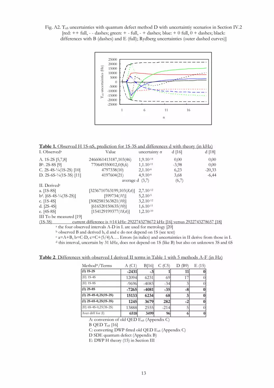
Fig. A2. TnS uncertainties with quantum defect method D with uncertaintiy scenarios in Section IV.2 [red: ++ full, - - dashes; green: + - full, - + dashes; blue: + 0 full, 0 + dashes; black:

differences with B (dashes) and E (full); Rydberg uncertainties (outer dashed curves)]

Table 1. Observed H 1S-nS, prediction for 1S-3S and differences d with theory (in kHz) I. Observeda Value uncertainty σ d [16] d [18]

A. 1S-2S [5,7,8] 2466061413187,103(46) 1,9.10-14 0,00 0,00 Bb. 2S-8S [9] 770649350012,0(8,6) 1,1.10-11 -3,98 0,00 C. 2S-4S-¼(1S-2S) [10] 4797338(10) 2,1.10-6 6,23 -20,33 D. 2S-6S-¼(1S-3S) [11] 4197604(21) 4,9.10-6 3,68 -6,44 average d (3,7) (6,7) II. Derivedc a. [1S-8S] [3236710763199,103(8,6)] 2,7.10-12 bd. [6S-4S-¼(3S-2S)] [599734(31)] 5,2.10-5 c. [1S-4S] [3082581563821(10)] 3,2.10-12 d. [2S-4S] [616520150635(10)] 1,6.10-11 e. [4S-8S] [154129199377(18,6)] 1,2.10-10 III To be measured [19] (1S-3S) current difference is ≈14 kHz: 2922743278672 kHz [16] versus 2922743278657 [18] a the four observed intervals A-D in I. are used for metrology [20] b observed B and derived b, d and e do not depend on 1S (see text) c a=A+B, b=C-D, c=C+(5/4)A…. Errors (in italics) and uncertainties in II derive from those in I. d this interval, uncertain by 31 kHz, does not depend on 1S (like B) but also on unknown 3S and 6S

Table 2. Differences with observed I derived II terms in Table 1 with 5 methods A-F (in Hz)

Method*/Terms A (C1) B[16] C (C5) D (B9) E (15) (I) 1S-2S -2431 -3 1 11 0 (II) 1S-4S 12094 6231 69 17 0 (II) 1S-8S -9696 -4083 -34 3 0 (I) 2S-8S -7265 -4081 -35 -8 0 (I) 2S-4S-0,25(1S-2S) 15133 6234 68 3 0 (I) 2S-6S-0,25(1S-3S) 1245 3679 282 -2 0 (II) 6S-4S-0,25(3S-2S) 13888 2555 -214 5 0 Aver diff for (I) 6518 3499 96 6 0

A: conversion of old QED EnS (Appendix C) B QED TnS [16] C: converting DWP fitted old QED EnS (Appendix C) D SDE quantum defect (Appendix B) E: DWP H theory (15) in Section III

-25000

-20000

-15000

-10000

-5000

0

5000

10000

15000

20000

25000

1 6 11 16

n

Tn

S un

cert

ain

ties

(H

z)

14

Table 3. TnS with uncertainties for n up to 20 using methods B (QED [16]) and D-E, this work

n B QED [16] D: (B9) this work E DWP (15) this work 1 2 82 258.954 399 283 2(15) 82 258.954 399 280 8(28) 82 258.954 399 283 1(0) 3 97 492.221 724 658(46) 97 492.221 724 005 8(3270) 97 492.221 724 045 6(1000) 4 102 823.853 020 867(68) 102 823.853 021 075(333) 102 823.853 021 075(135) 5 105 291.630 940 843(79) 105 291.630 940 957(317) 105 291.630 940 964(151) 6 106 632.149 847 323(86) 106 632.149 847 282(304) 106 632.149 847 293(160) 7 107 440.439 331 863(91) 107 440.439 331 743(294) 107 440.439 331 749(165) 8 107 965.049 714 599(93) 107 965.049 714 463(287) 107 965.049 714 463(169) 9 108 324.720 545 876(95) 108 324.720 545 761(281) 108 324.720 545 753(171) 10 108 581.990 788 289(97) 108 581.990 788 215(278) 108 581.990 788 199(173) 11 108 772.341 556 766(98) 108 772.341 556 741(275) 108 772.341 556 718(174) 12 108 917.118 852 716(99) 108 917.118 852 744(272) 108 917.118 852 714(175) 13 109 029.789 582 86(10) 109 029.789 582 934(270) 109 029.789 582 897(176) 14 109 119.190 324 18(10) 109 119.190 324 303(269) 109 119.190 324 261(176) 15 109 191.314 256 35(10) 109 191.314 256 518(268) 109 191.314 256 471(177) 16 109 250.342 392 65(10) 109 250.342 392 860(267) 109 250.342 392 809(177) 17 109 299.263 455 09(10) 109 299.263 455 344(265) 109 299.263 455 289(178) 18 109 340.259 771 78(10) 109 340.259 772 069(265) 109 340.259 772 011(178) 19 109 374.954 945 76(10) 109 374.954 946 078(265) 109 374.954 946 016(178) 20 109 404.577 117 11(10) 109 404.577 117 457(264) 109 404.577 117 393(178) ∞(-E1S) 109 678.771 743 07 109 678.771 743 809(260) 109 678.771 743 712(180) [redirection of E1S 0,001 109 331 26 0,000 994 964 037]

Table 4. Critical data for H Mexican hat curves with methods B-E and Kelly data [17]

Method Rharm(cm-1) nc(S) based on 4th order in 1/n B: recent QED 109679,350059184 1,572621509 from TnS in [16] C: older QED 109679,351984641 1,572663125 from EnS [17], eqn (C5) D: SDE 109679,3502083 1,572318726 from eqn (B10) E: DWP 109679,350018514 1,572665476 from eqn (15) [Kelly 109679,350325 1,572373 from TnS [17], eqn (D1)]