Precision Enhancement of MALDI-TOF-MS Using High ResolutionPeak Detection and Label-Free Alignment*

Maureen B. Tracy1,2, Haijian Chen3, Dennis M. Weaver4, Dariya I. Malyarenko5, MaciekSasinowski2, Lisa H. Cazares6, Richard R. Drake6, O. John Semmes6, Eugene R. Tracy3, andWilliam E. Cooke3

1 William and Mary Research Institute, College of William and Mary (CWM), Williamsburg, VA 23187-8795

2 INCOGEN, Inc., Williamsburg, VA 23188

3 Department of Physics, CWM, Williamsburg, VA 23187-8795

4 Saint Leo University, Langley Center, Hampton, VA

5 Department of Applied Science, CWM, Williamsburg, VA 23187-8795

6 Center for Biomedical Proteomics, Department of Microbiology and Molecular Cell Biology, EasternVirginia Medical School, Norfolk, VA

AbstractWe have developed an automated procedure for aligning peaks in multiple TOF spectra thateliminates common timing errors and small variations in spectrometer output. Our methodincorporates high resolution peak detection, re-binning and robust linear data fitting in the timedomain. This procedure aligns label-free (uncalibrated) peaks to minimize the variation in eachpeak’s location from one spectrum to the next, while maintaining a high number of degrees offreedom. We apply our method to replicate pooled-serum spectra from multiple laboratories andincrease peak precision (t/σt) to values limited only by small random errors (with σt less than onetime count in 89 of 91 instances, 13 peaks in 7 data sets). The resulting high precision allowed foran order of magnitude improvement in peak m/z reproducibility. We show that the CV for m/z is0.01% (100 parts per million) for 12 of the 13 peaks that were observed in all data sets between 2995and 9297 Da.

KeywordsAlgorithm; Mass Spectra; Mass Spectrometry; Reproducibility

1 IntroductionProtein expression profiling using MALDI-TOF-MS is a widely used technique for a varietyof studies including microbial typing [1], semi-quantitative comparison [2], imaging MS [3],etc. While advances in signal processing and instrumentation improve the ability to resolvespectral features, the reproducibility of such spectra remains a major limitation to the precisionof MALDI-TOF-MS. Precise time measurement is critical to both protein identification andpattern recognition in mass spectra. In order to achieve high precision, it is necessary to align(or synchronize) spectra so that characteristic features occur at the same time in all spectrabeing analyzed.

Correspondence: Dr. William E. Cooke, Professor of Physics, Department of Physics, Small Hall, College of William and Mary,Williamsburg, VA 23187-8795, USA. E-mail: wecook@wm.edu. Tel.: (757) 221-3512; Fax: (757) 221-3540.

NIH Public AccessAuthor ManuscriptProteomics. Author manuscript; available in PMC 2009 April 1.

Published in final edited form as:Proteomics. 2008 April ; 8(8): 1530–1538.

NIH

-PA Author Manuscript

NIH

-PA Author Manuscript

NIH

-PA Author Manuscript

Instrument precision can be reduced by both systematic and random errors. Although it is hardto avoid random errors, systematic errors can be reduced or eliminated from individual spectra,provided they can be characterized. The most important sources of systematic instrumentalerror in MALDI spectra are variations in the triggering time from spectrum to spectrum andsmall variations in the accelerating voltage. Since these errors appear as linear effects in theTOF data, it should be straightforward to remove such errors using corrections to uncalibratedTOF data.

There are various approaches to aligning TOF data including the use of: frequent calibration[4,5]; clustering or re-binning [6–13]; cross-correlations [14,15]; minimizing entropy [16,19];and others [17–24]. Of these, only three are based in the time domain, either directly [24] orindirectly by adjusting calibration parameters [16,23]. Corrections made in the time domainshould be inherently more accurate since m/z values are derived from equations obtained by aquadratic fit to a few calibration peaks in time data. (Corrections to data after calibration ineffect fit predicted values rather than measured values.)

In this study, we reanalyze the raw TOF data obtained during a multi-lab reproducibility study[25] using our high resolution peak detection and label-free alignment methods to show animprovement of more than an order of magnitude in precision. In this paper, label-freealignment refers to aligning time domain data by using the most commonly occurring peaks,without regard to the identity of those peaks. While we have used naturally occurring peaks,it would be possible to use markers that were added for calibration. However, even for addedcalibration markers, the actual m/z values would not be used for this alignment. This methodof label-free alignment should be broadly applicable and have significant impact for researchersusing TOF data for expression pattern analysis, imaging MS, and improved MS/MS proteinID.

2 Materials and Methods2.1 Data source

A multi-institution assessment of platform reproducibility has recently characterized theperformance of SELDI-TOF instruments at six different locations [25]. In this previous study,using stringent procedures for calibration/synchronization and standardization, six laboratoriesobtained inter-laboratory reproducibility approaching the intra-laboratory reproducibility.Quality Control (QC) samples were prepared using pooled normal human sera from 360 healthyindividuals (197 women and 163 men) and provided to all the sites. Each site then collectedTOF mass spectra from these QC samples and data were processed at a central site. Peaks wereidentified by locating local maxima and aligned by locating clusters of peaks within the‘window of potential shift’ ( m/z = 0.2% ) for each value of m/z [6] The synchronization andstandardization process included strict acceptance criteria with tolerances (for m/z resolution,intensity values and signal-to-noise ratios) prescribed for three omnipresent peaks ( m/z = 5910,7773 and 9297 Da). Following synchronization and standardization, 96 QC replicates were runat each site to evaluate the data reproducibility. During this subsequent evaluation, the threetarget peaks were shown to have CVs for m/z of 0.1%. For this paper, we have reprocessed theraw post-standardization TOF data from this multi-lab reproducibility study using the stepsoutlined below.

2.2 Label-free alignment of a single data setPrior to aligning data sets from different sites, we aligned the individual data sets separately.Figure 1 provides a schematic of our alignment procedure. The steps are described below.

Tracy et al. Page 2

Proteomics. Author manuscript; available in PMC 2009 April 1.

NIH

-PA Author Manuscript

NIH

-PA Author Manuscript

NIH

-PA Author Manuscript

Step 1: Detection of peak locations using a maximum likelihood method—Weremoved the slowly varying background using a charge accumulation model [15] and detectedpeaks using a maximum likelihood method [26]. This required fitting the data to a theoreticalline shape (a symmetric Gaussian of a specified width) centered in a sliding window. Since thepeak width in time units is nearly constant over a wide range of masses near the delayedextraction mass focused optimum (2–10 kDa, which covered the range of this study), we useda constant window width equal to the peak full width at half maximum (FWHM). (For highervalues of m/z, the peak width increases rapidly and the method must be adapted.[27].) We useda hypothesis test to locate windows that could contain peaks, and then maximized the likelihoodfunction to find the optimum window location (and thus peak location). To minimize the effectof line shape errors, we used only data within ±½ FWHM of the center of the line. While thismethod will fail if there are too many overlapping peaks, it easily detects equal intensity peaksseparated by at least one FWHM. All of the peaks reported in this paper were sufficientlyseparated from adjacent peaks to be resolved. We had the option of using either a Gaussiannoise model or a pseudo-Poisson noise model in our likelihood function. For the resultspresented in this paper, the latter noise model was used. A valuable byproduct of this maximumlikelihood approach was the routine estimation of the uncertainty in the peak position, σt. Aswill be discussed, this is a meaningful estimate of the random error in the peak position and

was typically a fraction of a clock count. The ratio provided an estimate of themass precision of the series of time measurements. While we used our peak detection method,the following alignment procedure (steps 2 – 5) can be applied to peak lists obtained by othermethods.

Step 2: Restricting the detected peak lists—Our peak detection method often foundlarge numbers of peaks, including many that could be quite small. We chose not to use intensityinformation directly, because we expected that to vary from one patient to another within aclinical data set. However, when the peak density was too high, alignment could becomeunstable with peaks at almost every time value (across the data set). So, we reduced the peaklist by restricting it to commonly occurring isolated peaks. We did this by creating a histogramof peaks for a data set and, using a bin width equal to our largest expected time shift in a dataset (±20 time steps in this work), we identified bins that contained at least 80% of the maximumnumber of counts (total number of spectra) with adjacent bins containing less than 40% of themaximum number. We then created shortened peak lists for each sample by only includingthose peaks that were counted in the selected bins in the histogram. A sufficient number ofpeaks were retained to insure correct matching of peaks between spectra. For this study, eightpeaks were included in the reduced peak list used to determine the correction factors. (Usingeight peaks to determine two correction parameters was sufficient to prevent over-correctionof the data.)

Step 3: Re - binning peak locations to construct a master list of common peaks—With the shortened peak lists, we constructed a master list of common peaks using aniterative process that delimits spectral regions without peaks. We began by choosing a largewindow size (typically the maximum expected shift which for this study was 8 times theFWHM) and excluding regions larger than that window in which no spectrum had peaks. Thisusually left some regions with peaks that were larger than the desired window size. We dividedany such large regions into two parts at the largest gap between peaks within ±1 window ofthe average position of the peaks in the bin. We repeated this until we reached the desiredwidow size (for this study, 3 times FWHM), and then eliminated any bins that had contributionsfrom too few spectra. For this study of nominally identical QC samples, we required bins tohave peaks from 80% of the available spectra. Finally, we generated a master peak list of theaverage position of all the measured values in each remaining bin.

Tracy et al. Page 3

Proteomics. Author manuscript; available in PMC 2009 April 1.

NIH

-PA Author Manuscript

NIH

-PA Author Manuscript

NIH

-PA Author Manuscript

Step 4: Determination of corrections to minimize the differences betweenreduced peak lists and the master list—The reduced peak list for each spectrum wasassigned a constant shift in time to minimize the average difference between its measuredlocations and the expected locations of the master list. The alignment procedure of Step 3 wasthen repeated to construct an improved master list. We then applied a robust linear fit to obtaincorrection factors for both offset and scale that would minimize the average difference betweenthe reduced peak lists and the expected locations of the new master list.

Step 5: Alignment of the original peak lists—We then applied the corrections obtainedin step 4 to the entire original peak lists, and then used the process of Step 3 with a desiredwindow size of the FWHM to construct a final master list of those bins with contributions fromat least 80% of the spectra. Since the alignment step introduced a scale and offset change toeach spectrum, re-binning could re-assign peaks to different bins when appropriate. At thecompletion of this process the bin size had been reduced to the size of a peak width and theresidual errors appeared to be random.

2.3 Label-free alignment of multiple data setsFor data sets collected on different dates or in different laboratories, preliminary steps wererequired to “roughly align” data sets prior to merging and aligning as a single data set. First, amaster peak list was obtained for each data set (steps 1 and 2 above) independently. (For thispreliminary master list construction, the inclusion criterion for peaks was relaxed fromoccurrence in 80% to 50% of the spectra.) Next, approximate time offsets and scale factorswere obtained (using least squares fit) to “roughly align” the master peak lists. After applyingthese corrections, we merged the data sets and the entire group was simultaneously re-binnedand aligned using the procedure above. This method was coded in C and R routines andimplemented as a custom R module within a commercially available visual bioinformaticsworkflow environment (VIBE, http://www.incogen.com). This module as well as theindependent routines can be downloaded from http://wecook.people.wm.edu.

3 Results and Discussion3.1 Alignment errors

Two types of systematic instrumental error are observed in TOF data: variations in thetriggering time from spectrum to spectrum and small variations in the accelerating voltage.Triggering time errors, or jitter between spectra, are differences in the measured TOF starttimes due to variations in the output from the digitizing clock and supporting analog electronics.These timing errors appear as constant time offsets in TOF spectra and are expected to be atleast ±1 time count. Since a triggering time error effects all time measurements in a spectrumequally, it can easily be eliminated by subtracting a constant from each time value. We observeoffsets as large at 12 clock counts within a single lab and as large as 62 clock counts betweenlaboratories. It is important to note that we are dealing with averaged spectra which are obtainedfrom multiple laser shots. Without access to individual spectra, it is impossible to completelyremove error due to jitter. The presence of time jitter between individual shots can producesplit peaks in the averaged spectra and consequentially produce errors in peak identification.The Appendix to this paper briefly describes this phenomenon. In addition to the start timejitter, any low frequency variation in the spectrometer acceleration voltage or any thermalexpansion (or contraction) of the time-of-flight tube can produce an apparent linear dilation orcontraction of the time measurement scale. As with the correction for jitter, a systematic errorof this type can be eliminated by simultaneously correcting all the points in a spectrum. Thistype of error can be corrected with a simple linear scale factor. We observe scale correctionswithin +/− 0.05%. For data taken during the same day at a given location we typically observecorrection factors of no more than 10−3. These correction factors are consistent with the

Tracy et al. Page 4

Proteomics. Author manuscript; available in PMC 2009 April 1.

NIH

-PA Author Manuscript

NIH

-PA Author Manuscript

NIH

-PA Author Manuscript

expected differences in power supply outputs in different instruments (1 part in a thousand).Figure 2 illustrates the offset and scale errors in two spectra obtained at one site on two differentdates. For this case, there is a 30 count offset and approximately a dilation of 0.007 (25 countsover 3600 counts). While frequent calibration can rectify these errors, it cannot remove theshot to shot voltage variations that occur due to pick-up of 60 Hz (line voltage) noise.

3.2 Typical peak displacements before and after label-free alignmentWe have analyzed 7 data sets, five containing 96 spectra each from 5 laboratories, the sixthcontaining 42 spectra from a single laboratory (Lab 2) and a seventh containing 522 spectrafrom all six laboratories combined. (A number of replicates in the data set from Laboratory 2data could not be used due to peak splitting revealed by our high resolution detection method.The appendix describes this problem.) For this study, 8 peaks in the range 2–10 kDa occur inat least 80% of the spectra prior to alignment and were used for the alignment procedure. Ofthe three target peaks used for the previous multi-lab study, only the m/z = 7773 Da peak wasincluded in the restricted peak list used to obtain correction factors for alignment in thisanalysis. The other two target peaks were not sufficiently isolated (as described in Section 2.2Step 2) to be included in the reduced peak list.

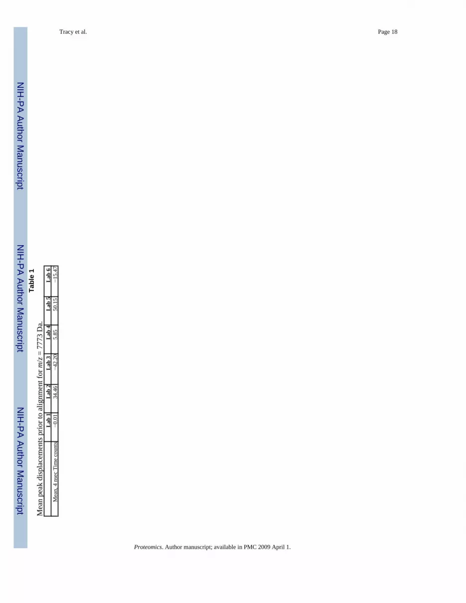
To illustrate the effectiveness of our alignment procedure, Figure 3 shows histograms of thepeak displacements (from the aligned time value) for the m/z = 7773 Da peak before (a) andafter (b) alignment. Prior to alignment, jitter between spectra appears as integer jumps in thepeak locations. Data from each lab clusters in the vicinity of its corresponding meandisplacement (indicated by vertical arrows) revealing systematic differences between the datasets. The mean for Lab 6 does not coincide with the center of a cluster because data from thislab is split between two clusters (at approximately −20 and +32) which were acquired on twooccasions, three months apart. (Data from Lab 6 required a preliminary step in which the dataobtained on the two different dates were “roughly aligned” as described in Section 2.3.) Table1 provides a numerical summary of the mean displacements. After alignment, the residualvariation in peak location is significantly smaller and appears random. This successfulalignment of data from 6 different sources without the application of calibrations demonstratesthe power of our time domain alignment method.

This large multi-lab data set allows us to obtain statistics on the performance of our alignmentprocedure. While comparable data sets from other instruments are not available to us, we havealso observed, and corrected, systematic time shift errors in standard spectra obtained using anUltraflex III MALDI-TOF (Bruker Daltonik) data [27].

3.3 Standard deviations for peak time locations following label-free alignmentFigure 4 presents standard deviations for peak time locations after alignment for 13 peaks thatare detected in all the data sets. The m/z values are obtained using a quadratic fit to the threetarget peaks identified in reference [25]. Peak location variability is reduced to below 1 timecount in 89 of 91 instances. The inter-laboratory variability (solid symbols) is comparable withthe intra-lab variability indicating that the alignment procedure has reached the limit ofprecision given the uncertainty predicted by maximum likelihood peak detection. The highervariability seen in the Lab 6 data set may be the result of the combination of two smaller datasets acquired on different days. The lower variability seen in the Lab 4 data results from ahigher sample rate used for data acquisition (twice the rate used by the other labs).

3.4 Relation between uncertainty in peak time location and S/NOne peak in Figure 4, t = 9663 counts, has a notably higher standard deviation than the others.This is due to a low S/N (peak signal divided by the root-mean-square noise in the window.)Figure 5 presents a portion of a typical spectrum that contains this peak and a neighboring peak

Tracy et al. Page 5

Proteomics. Author manuscript; available in PMC 2009 April 1.

NIH

-PA Author Manuscript

NIH

-PA Author Manuscript

NIH

-PA Author Manuscript

with a high S/N (t = 9621 counts, one of the peaks used for alignment process). Histogramsfor the residual peak displacements for both peaks provide insight into the alignment results.For these peaks, lower S/N is associated with higher uncertainty in the peak detection andgreater residual variation after alignment. Studies with simulated data show an inverse

relationship between σt and Here n is the number of time points inFWHM and C is a constant of order 1. This agrees with the theory of the peak detection method.

3.5 Random residual errors after label-free alignmentIn order to determine if the residual peak displacements are random or might still containsystematic errors, displacement histograms are fit to probability density functions. Figure 6presents histograms for four peaks with a t probability density function overlaid. The two plotson the left, a) and c), correspond to peaks used for label-free alignment (included in the reducedpeak list) and the two plots on the right, b) and d), correspond to peaks to which correctionswere applied (included in the original peak lists but not in the reduced peak list used fordetermination of correction coefficients). All show good agreement with a t -distribution whichsupports our claims that the residual displacements after alignment are random and systematictiming errors between spectra have been removed. The use of a t -distribution rather than anormal distribution is appropriate for modeling aligned peak values which are effectively meanquantities. [28]

3.6 CVs for peak m/z after label-free alignmentLow peak position uncertainty leads to remarkably high precision, as shown in Figure 7. Forthis figure, we translate the values for time precision into coefficients of variation for mass

using . (The factor of 2 arises from the fact that m/z values are obtained byapplying a quadratic calibration equation.) For reference, Figure 7 shows the previouslypublished CV values (marked as X’s) for the three target peaks used for synchronization in themulti-lab standardization study [25]. A logarithmic scale is used to highlight the order ofmagnitude improvement is precision. For convenience, Table 2 reproduces the CV values forthe 13 peaks detected in all data groups. Published values for the three target peaks from [25]are included and the peaks used for label-free alignment are indicated.

4 Concluding RemarksWe have shown significant improvements to TOF precision and, consequently, reproducibilityin m/z using linear time domain methods. Peak detection with superior resolution isdemonstrated and systematic instrument errors are identified and removed using linear offsetand scale corrections. We expect that our post-acquisition data processing will have significantimpact for researchers utilizing TOF data for expression pattern analysis, imaging MS, andimproved MS/MS protein ID.

Acknowledgements

The authors gratefully acknowledge D. Manos at the College of William and Mary for stimulating discussions. Thiswork was supported by NIH-National Cancer Institute grants CA101479 (MS), CA126118 (DIM) and CA085067(OJS).

AbbreviationsFWHM

peak full width at half maximum amplitude

ppm

Tracy et al. Page 6

Proteomics. Author manuscript; available in PMC 2009 April 1.

NIH

-PA Author Manuscript

NIH

-PA Author Manuscript

NIH

-PA Author Manuscript

parts per million

QC quality control pooled-serum

m/z precision, the inverse of CV

S/N peak signal divided by root-mean-square noise in window

t/σt time precision

σm/z uncertainty (SD) in peak location in m/z

σt uncertainty (SD) in peak location in time

References1. Fenselau C, Demirev PA. Characterization of intact microorganisms by MALDI mass spectrometry.

Mass Spectrom Rev 2001 20;157–17110.1002/mas.100042. Oleschuk RD, McComb ME, Chow A, Ens W, et al. Characterization of plasma proteins adsorbed onto

biomaterials by MALDI-TOFMS. Biomaterials 2000;21:1701–1710. [PubMed: 10905411]3. Caprioli RM, Farmer TB, Gile J. Molecular imaging of biological samples: localization of peptides

and proteins using MALDI-TOF MS. Anl Chem 1997;69(23):4751–4760.4. Chaurand P, DaGue BB, Pearsall RS, Threadgill DW, Caprioli RM. Profiling proteins from

azoxymethane-induced colon tumors at the molecular level by matrix-assisted laser desorption/ionization mass spectrometry. Proteomics 2001;1:1320–1326. [PubMed: 11721643]

5. Petricoin EF, Ardekani AM, Hitt BA, Levine PJ, et al. Use of proteomic patterns in serum to identifyovarian cancer. Lancet 2002;359:572–577. [PubMed: 11867112]

6. Yasui Y, McLerran D, Adam BL, Winget M, et al. An automated peak identification/calibrationprocedure for high-dimensional protein measures from mass spectrometers. J Biomed Biotechnol2003;4:242–248.10.1155/S111072430320927X [PubMed: 14615632]

7. Adam BL, Qu Y, Davis JW, Ward MD, et al. Serum protein fingerprinting coupled with a pattern-matching algorithm distinguishes prostate cancer from benign prostate hyperplasia and healthy men.Cancer Res 2002;62(13):3609–3614. [PubMed: 12097261]

8. Won Y, Song H-J, Kang TW, Kim J-J, et al. Pattern analysis of serum proteome distinguishes renalcell carcinoma from other urologic diseases and healthy persons. Proteomics 2003;3:2310–2316.10.1002/pmic.200300590 [PubMed: 14673781]

9. Ressom HW, Varghese RS, Abdel-Hamid M, Eissa SAL, et al. Analysis of mass spectral serum profilesfor biomarker selection. Bioinformatics 2005;21(21):4039–4045.10.1093/bioinformatics/bti670[PubMed: 16159919]

10. Yanagisawa K, Shyr Y, Xu BJ, Massion PP, et al. Proteomic patterns of tumour subsets in non-small-cell lung cancer. Lancet 2003;362:433–439. [PubMed: 12927430]

11. Tibshirani R, Hastie T, Narasimhan B, Soltys S, et al. Sample classification from protein massspectrometry, by ‘peak probability contrasts’. Bioinformatics 2004;20(17):3034–3044.10.1093/bioinformatics/bth357 [PubMed: 15226172]

12. Kazmi SA, Ghosh S, Shin DG, Hill DW, Grant DF. Alignment of high resolution mass spectra:development of a heuristic approach for metabolomics. Metabolomics 2006;2(2):75–83.10.1007/s11306–006–0021–7

Tracy et al. Page 7

Proteomics. Author manuscript; available in PMC 2009 April 1.

NIH

-PA Author Manuscript

NIH

-PA Author Manuscript

NIH

-PA Author Manuscript

13. Beyer S, Walter Y, Hellmann J, Kramer PJ, et al. Comparision of software tools to improve thedetection of carcinogen induced changes in the rat liver proteome by analyzing SELDI-TOF-MSspectra. J Proteome Res 2006;5:254–261.10.1021/pr050279o [PubMed: 16457590]

14. Rai AJ, Stemmer PM, Zhang Z, Adam BL, et al. Analysis of human proteome organization plasmaproteome project (HUPO PPP) reference specimens using surface enhanced laser desorption/ionization-time of flight (SELDI-TOF) mass spectrometry: multi-institution correlation of spectraand identification of biomarkers. Proteomics 2005;5:3467–3474.10.1002/pmic.200401320[PubMed: 16052624]

15. Malyarenko DI, Cooke WE, Adam B-L, Malik G, et al. Enhancement of sensitivity and resolution ofsurface-enhanced laser desorption/ionization time-of-flight mass spectrometric records for serumpeptides using time-series analysis techniques. Clin Chem 2005;51(1):65–74. [PubMed: 15550476]previously published online at DOI:10.1373/clinchem.2004.037283

16. Villanueva J, Philip J, DeNoyer L, Tempst P. Data analysis of assorted serum peptidome profiles.Nature Protocols 2007;2(3):588 – 602.previously published online at DOI:10.1038/nprot.2007.57

17. Baggerly KA, Morris JS, Coombes KR. Reproducibiliy of SELDI-TOF protein patterns in serum:comparing data sets from different experiments. Bioinformatics 2004;20(5):777–785.10.1093/bioinformatics/btg484 [PubMed: 14751995]

18. Dekker LJ, Dalebout JC, Siccama I, Jenster G, et al. A new method to analyze matrix-assisted laserdesorption/ionization time-of-flight peptide profiling mass spectra. Rapid Commun Mass Spectrom2005;19:865–870. [PubMed: 15724237]10.1002/rcm.1864

19. Villanueva J, Philip J, Chaparro CA, Li Y, et al. Correcting common errors in identifying cancer-specific serum peptide signatures. J Proteome Res 2005;4:1060–1072. [PubMed: 16083255]10.1021/pr050034b

20. Wong JWH, Cagney G, Cartwright HM. SpecAlign-processing and alignment of mass spectradatasets. Bioinformatics 2005;21(9):2088–2090. [PubMed: 15691857]10.1093/bioinformatics/bti300

21. Yu W, Wu B, Lin N, Stone K, et al. Detecting and aligning peaks in mass spectrometry data withapplications to MALDI. Comput Biol Chem 2006;30:27–38. [PubMed: 16298163]10.1016/j.compbiolchem.2005.10.006

22. Yu W, Li X, Liu J, Wu B, et al. Multiple peak alignment in sequential data analysis: a scale-space-based approach. IEEE/ACM Trans Comput Biol Bioinform 2006;3(3):208–219. [PubMed:17048459]

23. Jeffries N. Algorithms for alignment of mass spectrometry proteomic data. Bioinformatics 2005;21(14):3066–3073. [PubMed: 15879456]10.1093/bioinformatics/bti482

24. Lin SM, Haney RP, Campa MJ, Fitzgerald MC, et al. Characterizing phase variations in MALDI-TOF data and correcting them by peak alignment. Cancer Informatics 2005;1:32–40.http://la-press.com/cr_data/files/f_CI-1-1-LinSc_222.pdf

25. Semmes OJ, Feng Z, Adam BL, Banez LL, et al. Evaluation of serum protein profiling by surface-enhanced laser desorption/ionization time-of-flight mass spectrometry for the detection of prostatecancer: I. assessment of platform reproducibility. Clin Chem 2005;51:1,102–112. [PubMed:15613701]previously published online at DOI:10.1373/clinchem.2004.038950

26. Tracy, ER.; Chen, H.; Cooke, WE. Automatic peak identification method. U.S. Patent No. 7,219,038,May 15, 2007 (Assigned to the College of William and Mary)

27. Gatlin-Bunai CL, Cazares LH, Cooke WE, Semmes OJ, Malyarenko DI. Optimization of MALDI-TOF MS detection for enhanced sensitivity of affinity-captured proteins spanning a 100 kDa massrange. J Proteome Res. 200710.1021/pr0703526ASAP Article

28. Sivia, DS. Data Analysis: A Bayesian Tutorial. Oxford University Press; New York: 1996.

Appendix: Split spectra due to jitterTriggering time error cannot be completely removed because each spectrum is itself the averageof many laser shots, each with its associated jitter.[15] Without access to data from individuallaser shots, it is therefore impossible to completely remove all triggering time error. Smalltiming jitter in averaged spectra usually appears as peak broadening, but sometimes the

Tracy et al. Page 8

Proteomics. Author manuscript; available in PMC 2009 April 1.

NIH

-PA Author Manuscript

NIH

-PA Author Manuscript

NIH

-PA Author Manuscript

triggering jitter can jump between two widely separated vales, and this will split each peak intotwo (or more). Peak splitting due to timing jitter is distinguished from that resulting from thepresence of chemical adducts by the fact that each peak is split by the same constant timeincrement over the entire TOF spectrum (from the low mass sodium peak, through the matrixregion and throughout the mass focusing range). Figure A1 illustrates an egregious exampleof this timing jitter error in averaged spectra obtained at one site. The dotted line representstwo peaks from one spectrum that appears to have little jitter, while the solid line representsthe corresponding peaks from another spectrum that exhibits significant jitter. The clearly splitpeaks suggest that there are two main trigger start times associated with the single shot spectraand that the split spectra could be modeled as the average of two subgroups with different starttimes. A simulated split spectrum similar to the one in the figure is constructed by averaging110 copies of the unsplit spectrum and 90 copies with a delayed start time of 12 clock ticks.The agreement we see between the simulated peaks (shown as X markers) and the observedsplit peaks is consistent for all the peaks in the split spectrum. Differences in amplitude are tobe expected due to normal peak amplitude variations among replicates. To date, such peaksplitting has not challenged the vendor software for peak detection and clustering alignment.However, our new high resolution peak detection method exposes this problem as an obstacleto alignment and improved precision. For this paper, spectra with split peaks are not includedin the analysis and as a result, only 42 spectra for Lab 2 are analyzed.

Figure A1.Timing jitter in averaged MALDI-TOF spectra. The dotted and solid lines represent tworeplicate spectra (averages of 200 shots each). To illustrate that the split spectra can arise from

Tracy et al. Page 9

Proteomics. Author manuscript; available in PMC 2009 April 1.

NIH

-PA Author Manuscript

NIH

-PA Author Manuscript

NIH

-PA Author Manuscript

bimodal jitter, a simulated spectrum (represented by X’s) was generated by averaging copiesof the dotted spectrum with one of two start times. The solid dots show the difference betweenthe observed (solid line) and the simulated spectra.

Tracy et al. Page 10

Proteomics. Author manuscript; available in PMC 2009 April 1.

NIH

-PA Author Manuscript

NIH

-PA Author Manuscript

NIH

-PA Author Manuscript

Figure 1.Schematic of alignment procedure incorporating high resolution peak detection (step 1),selection of isolated common peaks (step 2), re-binning reduced peak list (step 3), robust lineardata fitting in the time domain (step 4), and alignment of original peak lists using correctionsfrom step 4 and re-binning to achieve a bin size of FWHM (step 5).

Tracy et al. Page 11

Proteomics. Author manuscript; available in PMC 2009 April 1.

NIH

-PA Author Manuscript

NIH

-PA Author Manuscript

NIH

-PA Author Manuscript

Figure 2.Evidence of trigger error (time offset) and voltage variation (time scale dilation) in spectrataken 3 months apart. The offset is 30 counts and the dilation is approximately 0.007 (25 countsover 3600 counts).

Tracy et al. Page 12

Proteomics. Author manuscript; available in PMC 2009 April 1.

NIH

-PA Author Manuscript

NIH

-PA Author Manuscript

NIH

-PA Author Manuscript

Figure 3.Histograms for m/z = 7773 Da peak displacements from aligned peak location for combineddata set. (a) Before alignment, integer jumps show clock jitter. Mean displacements forindividual labs are indicated by vertical arrows. (See Table 1 for numerical summary of meansand standard deviations.) (b) After alignment, residual displacements are small and random.Note the change of scale. (This peak was used for alignment in both reference [25] and thisstudy).

Tracy et al. Page 13

Proteomics. Author manuscript; available in PMC 2009 April 1.

NIH

-PA Author Manuscript

NIH

-PA Author Manuscript

NIH

-PA Author Manuscript

Figure 4.Standard Deviation in peak time locations following alignment. Variability is reduced to below1 time count for most cases. Inter-laboratory variability is comparable to intra-laboratoryvariability.

Tracy et al. Page 14

Proteomics. Author manuscript; available in PMC 2009 April 1.

NIH

-PA Author Manuscript

NIH

-PA Author Manuscript

NIH

-PA Author Manuscript

Figure 5.Histograms illustrating successful alignment of two peaks with different S/Ns. The peak at t =9621 was used for alignment in reference [25] and in this study. The peak at t = 9663 has asignificantly lower S/N and associated higher location uncertainty.

Tracy et al. Page 15

Proteomics. Author manuscript; available in PMC 2009 April 1.

NIH

-PA Author Manuscript

NIH

-PA Author Manuscript

NIH

-PA Author Manuscript

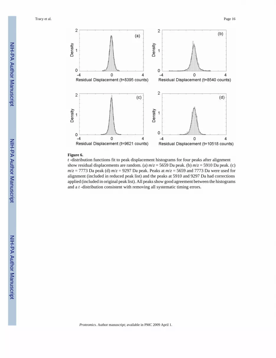
Figure 6.t -distribution functions fit to peak displacement histograms for four peaks after alignmentshow residual displacements are random. (a) m/z = 5659 Da peak. (b) m/z = 5910 Da peak. (c)m/z = 7773 Da peak (d) m/z = 9297 Da peak. Peaks at m/z = 5659 and 7773 Da were used foralignment (included in reduced peak list) and the peaks at 5910 and 9297 Da had correctionsapplied (included in original peak list). All peaks show good agreement between the histogramsand a t -distribution consistent with removing all systematic timing errors.

Tracy et al. Page 16

Proteomics. Author manuscript; available in PMC 2009 April 1.

NIH

-PA Author Manuscript

NIH

-PA Author Manuscript

NIH

-PA Author Manuscript

Figure 7.Coefficient of Variability for aligned peaks m/z values. Time domain alignment improvesprecision by at least an order of magnitude.

Tracy et al. Page 17

Proteomics. Author manuscript; available in PMC 2009 April 1.

NIH

-PA Author Manuscript

NIH

-PA Author Manuscript

NIH

-PA Author Manuscript

NIH

-PA Author Manuscript

NIH

-PA Author Manuscript

NIH

-PA Author Manuscript

Tracy et al. Page 18Ta

ble

1M

ean

peak

dis

plac

emen

ts p

rior t

o al

ignm

ent f

or m

/z =

777

3 D

a.L

ab 1

Lab

2L

ab 3

Lab

4L

ab 5

Lab

6M

ean,

4 n

sec

Tim

e co

unts

−0.0

134

.46

−42.

205.

8550

.15

−15.

47

Proteomics. Author manuscript; available in PMC 2009 April 1.

NIH

-PA Author Manuscript

NIH

-PA Author Manuscript

NIH

-PA Author Manuscript

Tracy et al. Page 19

Table 2Coefficients of variation for peak m/z.

Peaksa) m/z CV, %m/z, Da Time counts Label-free alignment Ref [25]2995 6879b) 0.00943485 7155b) 0.00814941 7983b) 0.00905659 8395b) 0.00655910c) 8540 0.0110 0.117773c) 9621b) 0.0054 0.107845 9663 0.02027939 9719 0.00847989 9748 0.00998164 9850 0.01118630 10124b) 0.00848955 10316 0.00849297c) 10518 0.0067 0.11a)

Peaks detected in all data sets.

b)Peaks used for label-free alignment.

c)Target peaks from reference [25]

Proteomics. Author manuscript; available in PMC 2009 April 1.