Embed Size (px)
Citation preview

Predicting Viral Infection From High-Dimensional BiomarkerTrajectories
Minhua Chen, Aimee Zaas, Christopher Woods, Geoffrey S. Ginsburg, Joseph Lucas,David Dunson, and Lawrence CarinMinhua Chen is Ph.D. Student, Electrical and Computer Engineering Department, Aimee Zaas isAssociate Professor, Christopher Woods is Associate Professor, Geoffrey S. Ginsburg isProfessor and Director of Genomic Medicine, and Joseph Lucas is Assistant Research Professor,Institute for Genome Sciences and Policy & Department of Medicine, David Dunson is Professor,Department of Statistical Science, and Lawrence Carin is Professor and Department Chair([email protected]), Electrical and Computer Engineering Department, Duke University,Durham, NC 27708-0291
AbstractThere is often interest in predicting an individual’s latent health status based on high-dimensionalbiomarkers that vary over time. Motivated by time-course gene expression array data that we havecollected in two influenza challenge studies performed with healthy human volunteers, we developa novel time-aligned Bayesian dynamic factor analysis methodology. The time course trajectoriesin the gene expressions are related to a relatively low-dimensional vector of latent factors, whichvary dynamically starting at the latent initiation time of infection. Using a nonparametric cure ratemodel for the latent initiation times, we allow selection of the genes in the viral response pathway,variability among individuals in infection times, and a subset of individuals who are not infected.As we demonstrate using held-out data, this statistical framework allows accurate predictions ofinfected individuals in advance of the development of clinical symptoms, without labeled data andeven when the number of biomarkers vastly exceeds the number of individuals under study.Biological interpretation of several of the inferred pathways (factors) is provided.
KeywordsBayesian nonparametrics; Dynamic factor analysis; High-dimensional; Infectious disease; Jointmodel; Multidimensional longitudinal data; Multivariate functional data; Predictive model
1. INTRODUCTIONThere is much recent interest in the analysis of dynamic biological processes, particularlywith data from DNA gene expression microarray chips (Holter et al. 2001; James and Hastie2001; Bar-Joseph et al. 2003; Bar-Joseph 2004; Lawrence, Sanguinetti, and Rattray 2007;Liu et al. 2010). Treating the gene expression trajectories as functional data, Gaussian
© 2011 American Statistical Association
Full terms and conditions of use: http://www.tandfonline.com/page/terms-and-conditionsThis article may be used for research, teaching, and private study purposes. Any substantial or systematic reproduction, redistribution,reselling, loan, sub-licensing, systematic supply, or distribution in any form to anyone is expressly forbidden.The publisher does not give any warranty express or implied or make any representation that the contents will be complete or accurateor up to date. The accuracy of any instructions, formulae, and drug doses should be independently verified with primary sources. Thepublisher shall not be liable for any loss, actions, claims, proceedings, demand, or costs or damages whatsoever or howsoever causedarising directly or indirectly in connection with or arising out of the use of this material.
NIH Public AccessAuthor ManuscriptJ Am Stat Assoc. Author manuscript; available in PMC 2013 May 21.
Published in final edited form as:J Am Stat Assoc. 2011 January 1; 106(496): 1259–1279. doi:10.1198/jasa.2011.ap10611.
NIH
-PA Author Manuscript
NIH
-PA Author Manuscript
NIH
-PA Author Manuscript

process (Lawrence, Sanguinetti, and Rattray 2007; Liu et al. 2010) and spline-based models(James and Hastie 2001; Bar-Joseph et al. 2003) have been proposed. Appropriatelyanalyzing the trajectories as multivariate functional data is challenging because of themassive dimensionality, few observations in time, low signal-to-noise ratio, andmissingness. Ideally, methods would allow building of a full joint model that allows eachgene to have its own trajectory while accommodating dependence in these trajectories acrossgenes within shared pathways and variability across individuals. In the literature, theemphasis has been on clustering genes (James and Hastie 2001; Bar-Joseph et al. 2003) andon modeling each gene separately, possibly with shared covariance parameters (Liu et al.2010). In both of these constructions the objective is to share strength appropriately amongmultiple genes. Authors also have grouped genes via a singular value decomposition (SVD)(Holter et al. 2001), and have modeled the time dependence of the SVD modes via anautoregressive framework. In such time-dependent modeling, one often must distinguish theobserved (“wall clock”) time at which a measurement was performed from the (latent)biological clock time, and the difference between these two must be in- ferred (because theoffset between the two is typically subject-dependent) (James and Hastie 2001; Liu et al.2010).
As a separate line of research for analysis of genomic data (e.g., gene expression data),researchers have investigated factor analysis and related models (Lopes and West 2004;Zou, Hastie, and Tibshirani 2004; Carvalho et al. 2008). The factors group genes that arecoexpressed across multiple samples, and thus they constitute a generalization of SVDapproaches (West 2003). Grouping genes via factor loadings avoids the need to explicitlyimplement a clustering step (Bar-Joseph et al. 2003), and the factor loadings need not beconstrained by orthonormality restrictions (Holter et al. 2001). Furthermore, it is desirable toimpose the condition of sparse factor loadings (Zou, Hastie, and Tibshirani 2004; Carvalhoet al. 2008), with the goal of inferring compact biological pathways.
In this article we consider Bayesian factor analysis of time-evolving gene expression data.Our proposed model builds on previous research that has used spline-based approximationsto continuous-time data (James and Hastie 2001; Bar-Joseph et al. 2003). The use of factoranalysis obviates the need for explicit clustering (Bar-Joseph et al. 2003) of genes. Ratherthan modeling the time dependence of orthonormal (and not necessarily sparse) modes of anSVD construction (Holter et al. 2001), we model the time dependence of the factors, whichmay be related to biological functions and pathways. We also develop a novel means ofinferring the latent time shift of the biological process (Liu et al. 2010). An approximation tothe full posterior of model parameters is implemented via efficient Gibbs sampling. Afterintroducing the model in detail in Section 2, we highlight the novelty of the proposedapproach, by making further connections and relationships to the existing time-course geneexpression literature.
The analysis is motivated by and illustrated with a novel dataset that we measured in recentchallenge studies. Specifically, after receiving appropriate Institutional Review Boardapproval, we performed two separate challenge studies. For each, roughly 20 healthyindividuals were inoculated with a particular influenza virus, and blood samples werecollected at regular time intervals until the individuals were discharged. The specific virusesconsidered were two strains of influenza, H3N2 and H1N1 (discussed in further detailbelow). These data provide a unique opportunity to examine the time-evolving host responseto such viruses. The blood was assayed with DNA microarray technology to constitute geneexpression values for 12,023 genes, with which the time-evolving factor analysis wasperformed.
Chen et al. Page 2
J Am Stat Assoc. Author manuscript; available in PMC 2013 May 21.
NIH
-PA Author Manuscript
NIH
-PA Author Manuscript
NIH
-PA Author Manuscript

The remainder of the article is organized as follows. In Section 2 we introduce the time-evolving factor model, allowing subject-dependent jitter between the observed time and thelatent biological time. In Section 3 we examine the model using simulated data. In Section 4we present results based on analysis of time-evolving DNA microarray data, using data thatwe measured in two influenza challenge studies. In Section 5 we examine the model’sability to make predictions about held-out data samples. We provide a brief discussion of thebiological processes inferred from the model in Section 7, and conclude in Section 8.
2. MODELING TIME–EVOLVING FACTORS2.1 Basic Factor Model
Let Xi∈ ℝp×ni represent observed biomarkers (e.g., gene expression data) for individual i,considering p markers, collected at nitime points, with the jth column of Xi corresponding tothe p biomarkers measured at time tij, for j ∈ {1, …, ni}. We assume a total of I individuals,constituting cumulative data {Xi}i=1,I, where in general the number of samples ni and thespecific time points tij of measurements may be subject-dependent. We consider a factormodel with k factors
(1)
where L ∈ ℝp×k is the factor loading matrix, and Lm is the mth column of L; the factor
scores for individual i are Si ∈ ℝk×ni, and is a row vector (mth row of Si) of time-varyingscores for the ith individual and mth latent factor. The factor loadings are assumed fixed in
time, and the latent factors, , are allowed to vary dynamically. By assuming fixedloadings, we avoid having the meaning of the latent factors change with time and thus obtainresults that are more biologically interpretable. At this point, we assume fixed k; later wediscuss inference of the appropriate number of factors. The matrix Ei ∈ ℝp×ni is the additivenoise or residual.
2.2 Shifted Spline RepresentationThe principal modeling contribution of this article concerns the prior placed on the factorscores {Si}i=1,I. Recall that individual i has data sampled at ni time points; let ti = (ti1, ti2, …,tini) denote the time points at which data were collected for individual i (in units of minutes/hours, etc.), with respect to a time reference shared by all I individuals. Note that these areobserved times on a universal clock, to be distinguished from the latent biological clock ofthe system under investigation (in our specific example, corresponding to the host responseto a virus), which generally is individual-dependent. The rows of Si(t) are a continuousfunction of time, and the matrix Si represents each such row sampled at the ni time pointsrepresented by ti.
Recall that Smi ∈ ℝni represents the factor score associated with factor m ℝ {1, …, k} forsubject i ∈ {1, …, I}, evaluated at the ni discrete time points in ti (Smi is a column vector,
the transpose of above). To model Smi, let b(t) ∈ ℝq represent a column vector,corresponding to the evaluation of each of q spline functions at any time t over the supportof the splines (James and Hastie 2001; Bar-Joseph et al. 2003), defined here by the timewindow in which data are collected. The number of splines, q, and their composition dependon the specific application, as we discussed in more detail later. The function b(t − τ) ∈ ℝq
corresponds to realigning the spline functions to have the time origin shifted forward by τ ∈ℝ. We allow a time shift τmi specific to latent factor m and individual i by characterizing thefactor score trajectories as
Chen et al. Page 3
J Am Stat Assoc. Author manuscript; available in PMC 2013 May 21.
NIH
-PA Author Manuscript
NIH
-PA Author Manuscript
NIH
-PA Author Manuscript

(2)
where [B(ti;τmi)]⊤ = [b(ti1 − τmi), …, b(tini − τmi)], [B(ti; τmi)]⊤ is the transpose ofB(ti;τmi). Vector wm ∈ ℝq corresponds to the spline coefficients for the mth latent factor,
which is drawn as , with Iq the q × q identity matrix. This prior isequivalent to a ridge regression to regularize the B-splines for the latent factor. We furtherelucidate the detailed model construction later. Figure 1 illustrates the foregoing generativeprocess.
The expression B(ti; τmi)wm is meant to represent an underlying continuous-time signal forfactor m, sampled at discrete points defined by ti and shifted to the right by a subject-dependent time τmi. Note that the vector of spline weights wm for factor m is shared acrossall {Xi}i=1,I, and thus it seeks to model an underlying individual-independent biologicalprocess, with individual-dependent shift. The residual εmi captures differences between theshifted baseline signature B(ti; τmi)wm and the individual-dependent factor Smi. Because theunderlying shifted signal is approximated by continuous-time splines, once the splineweights wm are inferred based on the observed discrete data, we may make inferences aboutthe factor at any continuous time point over the support of the experiment.
2.3 Temporal Shift and Distinguishing Host-Response FactorsIn our motivating application, all individuals are inoculated with a virus at the same time.Blood is drawn from all subjects at a specified time before inoculation (t=−5 hours) toconstitute a baseline signature, and another (distinct) blood sample is drawn just beforeinoculation (defined as time t = 0 hours). The vector ti is defined such that increasingelement index corresponds to increasing time; this vector records the times at which bloodsamples were collected. Thus each individual shares the same first two time points in ti, andbecause the time of inoculation is by definition t = 0, the first element in ti corresponds tonegative time.
Because our objective is to study the host (body) response to the virus, our spline-basedconstruction for the time-dependent factors is constituted as in Figure 2. Note that thefunction B(ti;τmi = 0)wm has a constant form for t ≤ −5 hours (with value of the constantinferred via the analysis), representing the background/baseline (preinoculation) factor scorefor a (presumably) healthy individual. Consequently, with application to our challengestudies, the shift τmi may be viewed as the delay between inoculation of subject i and thetime at which factor m changes from its background (“normal”) value. This is the hostresponse time for pathway m, which is expected to vary between subjects. Related temporal-onset models have been considered by (Dunson and Baird 2002; Dunson et al. 2004).
A multinomial prior is imposed on τmi as
(3)
where λmj is the jth component of the probability vector λm and the Dirichlet distribution
hyperparameters are set as , where 1 is a T-dimensional vector of all 1s. The
; represent candidate (discretized) shifts, with increment Δ a specified small unitof time with positive value, and (T − 1) Δ covers the full range of anticipated shifts (theduration of the experiment). Although we have discretized the possible shifts in terms offinite Δ, for convenience, Δ may of course be made arbitrarily small to achieve a desired
Chen et al. Page 4
J Am Stat Assoc. Author manuscript; available in PMC 2013 May 21.
NIH
-PA Author Manuscript
NIH
-PA Author Manuscript
NIH
-PA Author Manuscript

level of modeling resolution. The choice of hyperprior is chosen to limit sensitivity to T, asconvergence to a Dirichlet process is obtained in the limit as T→∞). Model (3) is easilyadapted to include patient covariates that may affect the host response times by using acontinuation ratio probit or alternative discrete hazard regression model.
Considering Figure 2, note that large shifts τmi imply that individual i has a near-constanthost response for factor m as a function of time (“near,” but not exactly constant because ofthe addition of the εmi). This model is consistent with our influenza challenge study data,because approximately half of the individuals did not become symptomatic, and for theseindividuals, all of the associated factor scores demonstrated very weak temporal changes.Thus the presence of large τmi for all factors m ∈ {1, …, k} implies that individual i isasymptomatic. Furthermore, if a particular factor m ∈ {1, …, k} is not related to the hostresponse to the virus for individual i, then the associated τmi will be large, implying that Smiis nearly time-invariant. Along with considering the simple Dirichlet distribution prior in(3), we also considered a discrete-time hazard model with a surviving fraction (individualswho do not become symptomatic). Specifically, consider
(4)
where δ(j−1)Δ is a unit point measure at (j − 1) Δ. There are two motivations for theforegoing construction. First, the Stick(τmi; Δ) component favors small τmi, consistent withthe expectation that when the factor has a time-dependent response, the onset of the hostresponse is anticipated to be near the inoculation time (t = 0).With probability ζm, the mthfactor yields a time-dependent response, and with probability 1 − ζm, the factor is nearlytime-invariant. Although (4) captures more of our prior expectations, it involves moreparameters than the simple Dirichlet distribution construction in (3). Both (3) and (4)worked well in our experiments and generally yielded similar results; thus the data do notprovide sufficient evidence in favor of (4) over (3), and we focus on the simpler model inthe remainder of the article.
To complete the model for the factor scores in (2), we need to specify the draws of the term∈mi. We assume
(5)
Note that here we use a subject-dependent precision parameter φmi for the mismatchbetween the trajectory and the factor score. With this model flexibility, we allow thismismatch to be large for some subjects, leaving room for the outlier (atypical) subjects.
2.4 Sparse Factor LoadingsIn many biological applications, it is desirable to impose the condition that the factor-loading matrix is sparse (Carvalho et al. 2008). In the case of gene expression data, the mthfactor can be viewed as measuring overall expression of the mth pathway, with the nonzeroelements in the mth column of the loadings matrix Lm corresponding to the genes in thatpathway. Biologically, we would expect a small minority of the genes to play a role in anysingle pathway, implying sparsity. Thus we model the loading matrix as
Chen et al. Page 5
J Am Stat Assoc. Author manuscript; available in PMC 2013 May 21.
NIH
-PA Author Manuscript
NIH
-PA Author Manuscript
NIH
-PA Author Manuscript

(6)
where o represents a pointwise (Hadamard) matrix product between A ∈ ℝp×k and Z ∈ {0,1}p×k. The binary matrix Z is designed to be sparse, and thus the factor loadings, defined bythe columns of A o Z, are sparse as well.
The following priors are placed on the components of A and Z:
(7)
for g = 1, …, p and m = 1, …, k. The gth gene, g ∈{1, …, p}, contributes to factor m withprobability πm, and for those genes that have nonzero contribution, the loading is drawn
from normal . Thus if gene g does not contribute to the mth pathway, then itmakes no contribution to the corresponding factor loading (Agm = 0).
The basic form of (7), apart from the manner in which Si are analyzed, is the same as thatdeveloped by (Carvalho et al. 2008). Several alternatives may be considered, which we haveexamined in the course of this study. Here we summarize these augmentations and ourexperience with them. First, rather than using a “spike-slab” prior for the components of thefactor-loading matrix A o Z (West 2003; Carvalho et al. 2008) as in (7), one may imposesparseness (or approximate sparseness) on the factor loadings via shrinkage priors [e.g.,Student t (Tipping 2001) with heavy tails]. Such a construction does not impose explicitsparseness, but many components of the factor loadings will be negligibly small. We foundthat such constructions work as well as the model presented earlier, but we prefer to allowexact 0s for the interpretation of pathways and factors without the need to threshold theloadings
Our proposed construction also yields an interesting interpretation in terms of the Indianbuffet process (Griffiths and Ghahramani 2005; Thibaux and Jordan 2007; Rai and Daume2008; Paisley and Carin 2009). To understand this connection, define the hyperparameters tothe beta distribution in (7) as e0 = α0/k and f0 = β0/k, where k is the truncation level (upperbound) on the number of factors and α0 and β0 are positive real constants. Aftermarginalizing out {πm}m=1,k and taking the limit as k → ∞, we may interpret the model asfollows (Griffiths and Ghahramani 2005; Thibaux and Jordan 2007; Rai and Daume 2008;Paisley and Carin 2009). Each of the p genes are “customers” in a buffet restaurant, and theset of spline weights {wm}m=1,k and the precisions {βm}m=1,k, k→ ∞), represent potentialdishes; that is, wm and βm jointly represent the mth dish. If gene g selects dish m, then Zgm= 1; otherwise, Zgm = 0. The first gene enters the buffet and selects the first M1 ~Poisson(α0/β0) dishes; therefore, Z1m = 1 for m ∈ {1, …,M1} and Z1m = 0 for m > M1. Thesecond gene then comes into the buffet, and for m ∈ {1, …,M1}, Z2m ~ Bernoulli(1/(1 +β0)). In addition, Z2m = 1 for m ∈ {M1 +1, …,M1 +M2}, where M2 % Poisson(α0/α0 +1).This process continues sequentially, with each gene selecting from previously selecteddishes via a Bernoulli distribution and selecting newly used dishes via a Poissondistribution. After this has been done for the first p − 1 genes, assume that a total of
dishes have been selected, and that the mth dish has been selected nm timesby the previous p − 1 genes. Then for m ∈ {1, …, M̂p−1}, Zpm ~ Bernoulli(nm/(β0 + p − 1)).Furthermore, Zpm = 1 for m ∈ {M̂p−1+1, …,M̂p−1+Mp}, with Mp ~ Poisson(α0/(β0 +p −1)).
Chen et al. Page 6
J Am Stat Assoc. Author manuscript; available in PMC 2013 May 21.
NIH
-PA Author Manuscript
NIH
-PA Author Manuscript
NIH
-PA Author Manuscript

For those dishes m for which Zgm = 1, the gth gene draws an associated loading
, and AgmB(t;0)wm represents the time-dependent trajectory of this gene, ascontributed by factor m, apart from a subject-dependent shift τmi and noise εmi. This isdone for all factors used by gene g (i.e., all m for which Zgm = 1), and these are superposedto yield the total response of gene g contributed by the factors. Note that this prior isexchangeable (Griffiths and Ghahramani 2005; Thibaux and Jordan 2007), implying that itis insensitive to a permutation of the gene order.
We now report some observations regarding what this prior is imposing. Although in theforegoing discussion we considered the limit k→∞, the expected number of factors used is
, and this number is always finite. Note that as the gene index gincreases in the foregoing process, the probability of using unused dishes diminishes (via thePoisson distribution); this implies that after observing many genes, we likely will havecaptured most of the factors responsible for the associated expression representation.Finally, the model imposes the idea that the more popular particular dishes (factors) areamong the genes that came to the buffet previously, the greater the likelihood that asubsequent gene will select that factor. Thus the model imposes that there is likely a subsetof “popular” dishes/factors, but there is an opportunity for genes to have idiosyncratic factorusage.
Within the computations, one may explicitly integrate out the {πm}m=1,k and consider thelimit k→∞, rigorously (Rai and Daume 2008). However, for the large number of genes pconsidered here, we have found this approach to be computationally expensive. Therefore,in the results that follow we set k to a large value and allow the model to infer the subset offactors needed for representation of the data; thus the setting k does not reflect the numberof anticipated factors, but rather is a numerical upper bound.
All computations were performed using Gibbs sampling. The detailed equations arepresented in the Appendix A.
2.5 Relationships to Previous Time-Course Gene Expression ModelsNumerous previous studies have analyzed time-course gene expression data (Holter et al.2001; James and Hastie 2001; Bar-Joseph et al. 2003; Bar-Joseph 2004; Lawrence,Sanguinetti, and Rattray 2007; Liu et al. 2010), almost all of which used a clustering of thegenes. To model the continuous time dependence of the gene expression, researchers haveused the Gaussian process (Lawrence, Sanguinetti, and Rattray 2007; Liu et al. 2010), aswell as spline basis functions (James and Hastie 2001; Bar-Joseph et al. 2003) like thoseconsidered here. In this discussion we focus on the latter, because that work is most closelyconnected to our proposed model. Most of these methods use mixed-effects models that maybe expressed as
(8)
where xg(tij) represents the expression of the gth gene for subject i as observed at time tij.
The fixed-effects component, , corresponds to cluster c, with the genesclustered among one of C different classes or clusters. The random-effects term,
, has a continuous time dependence that is a function of the specific gene gand subject i. The expressions B̂l(tij) and Bl(tij) represent basis functions (typically splines)
evaluated at time tij, the and .γigl are basis function coefficients, and εgij accounts for
Chen et al. Page 7
J Am Stat Assoc. Author manuscript; available in PMC 2013 May 21.
NIH
-PA Author Manuscript
NIH
-PA Author Manuscript
NIH
-PA Author Manuscript

residual/noise. Hierarchical clustering of the genes (Heard, Holmes, and Stephens 2006)may be used as well.
Additional examples of such a mixed-effects clustering model applied to time-course geneexpression data include work of (Luan and Li 2003; Heard et al. 2005; Storey et al. 2005;Ng et al. 2006; Wang, Chen, and Li 2007; Scharl, Grun, and Leisch 2010). Although thisapproach has been applied successfully in many settings, it has certain limitations thatrestrict its utility. For example, we are typically interested in more than 10,000 genes whenperforming microarray analysis, and thus the number of spline-based expansions that mustbe fit is significant. In addition, for the application of interest here, we have on the order of20 different subjects, each manifesting a distinct time-course profile.
To the best of our knowledge, this article represents the first use of spline expansions withinthe context of factor analysis, with specific demonstration in terms of time-course geneexpression data. Given that the factor loadings have gene-dependent strengths, the factormodel yields a unique spline-based continuous signature for each gene and each subject.Specifically, our proposed model represents the gene- and subject-dependent time course as
(9)
Recalling that τmi is the shift for subject i and factor m, a maximum of k factors areconsidered, Zgm is the binary variable for gene g in factor m, Agm is the loading when Zgm =1, and wml is the lth spline weight for factor m. The number of factors used is typicallymuch smaller than the number of genes, and thus the number of spline coefficients that mustbe inferred is significantly less than that associated with (8). Note that there are two forms ofresiduals; εmi(tij) accounts for subject-dependent variation in the time-dependent factorscore, whereas Egi(tij) accounts for gene- and subject-dependent variation, of particularimportance when a given gene makes no contribution to the factor loadings.
Our proposed approach avoids the need to explicitly perform clustering (which is doneimplicitly within the factor loadings), and the shifts τmi yield subject-dependent continuous-time models for each gene. If gene g does not contribute significantly to the biology undertest, then Zgm = 0 for all factors m∈{1, …, k}. Typically only a small fraction of the genescontribute to the biology under study, but in (8) one explicitly infers (presumably negligible)spline coefficients for each of the numerous unimportant genes. In contrast, using theproposed model in (9), we only use splines to model the small number of factor scores (withsubject-dependent shifts).
3. SIMULATION STUDY3.1 Form of the Results
From (9),
(10)
represents the contribution of factor m to the expression of gene g, as viewed at time tij(subject i, time index j). When addressing the time trajectory of factor m, we consider one ofthe genes for which Zgm = 1 (one of the characteristic genes for factor m) and present the
statistics of based on the collection samples. The genes that contribute to this factorare distinguished only by the weighting Agm, and thus as long as Zgm ≠ 0, which gene g is
Chen et al. Page 8
J Am Stat Assoc. Author manuscript; available in PMC 2013 May 21.
NIH
-PA Author Manuscript
NIH
-PA Author Manuscript
NIH
-PA Author Manuscript

selected is not of particular importance. By considering , rather than the time-dependent factor score, we avoid scaling variability that may be manifested between theloading and score.
When computing the model parameter statistics, we must address the fact that the index ofthe factor may change between collection samples; it should change between collectionsamples if there is good mixing. When aggregating collection samples, we computecorrelations between the normalized time-dependent score of factor m at Gibbs collection swith the normalized factor scores of all factors for the first collected sample. If a factor fromsample s has a correlation exceeding 0.95 with factor m from the first collected sample, thenthese are deemed to be samples from the same factor. The results are not sensitive to the0.95 threshold, and this alignment of factors proved effective for both the simulated and realdata; for the simulated data, we were able to validate against truth. Related methods havebeen considered by Stephens (2000).
In addition, at some Gibbs iterations it is possible that a single factor may split into two, forexample, because
, for any ζgm. This splitting does not generally occur, but it can occur in some collectionsamples. When splitting did occur, it did so in the foregoing form. For each collectionsample, we also considered the interfactor correlations of the time-dependent factor scores.Within a particular collection sample, if two (or more) factor score trajectories are correlated
more than 0.95, then the total contribution to from that collection sample is the sumof the correlated terms. When presenting results on the inferred number of factors, we countthe unique factors after addressing this issue, if it should occur in a particular collectionsample.
Note that the time-dependent nature of the data—reflected in the corresponding shape of thefactor scores with time—has proven effective as a means of tracking factors within andbetween Gibbs collection samples. This is an attractive characteristic of time-evolving data,with such sample tracking less simple without multiple time points.
3.2 Synthetic DataWe synthesized data from the model, and then used the foregoing framework to infer thelatent parameters. Specifically, the data consisted of I = 20 subjects, with each subjectsampled randomly at ni = 16 time points (different, randomly selected time points for eachsubject). We considered a total of p = 1000 “genes,” resulting in a total data matrix ofdimension 1000 × 320. We also considered simulated data with p = 10,000, which is closerto the dimension of the real data, with similar inference quality manifested; however, suchhigh-dimensional data are harder to display, and thus we omit them here.
We generated the data matrix by four factors, with each factor loading (pathway) containing50 nonzero values. We generated the remaining 1000−50 · 4 = 800 genes by random noise,represented by Ei. The four factors for each subject are shifted and sampled versions of fourunderlying (“prototype”) trajectories, simulating four biological processes. The nonzerocontributions to the factor loadings were drawn iid from 0, 1), and the components of Eiwere also drawn from 0, 1). Thus the average strength of the gene expression for all genesare the same regardless of whether or not they contribute to the factor loadings.
For the model inference, an upper bound on the number of factors was k = 20 (although intruth only four factors were used to generate the data, but of course this was unknown to the
Chen et al. Page 9
J Am Stat Assoc. Author manuscript; available in PMC 2013 May 21.
NIH
-PA Author Manuscript
NIH
-PA Author Manuscript
NIH
-PA Author Manuscript
analysis). A total of 10,000 burn-in Gibbs iterations were performed, along with 10,000collection iterations.
In this synthesized example, we generated the B-spline basis using online source code http://www.nonlinear-approx.info/code/matlab/TSpline.m. We generated 10 B-spline functions oforder 3 with knot sequence length 13. Other parameter settings were as follows:
c0 = d0 = c1 = d1 = c2 = d2 = c3 = d3 = 10−6,
e0 = 10−3p, f0 = (1 − 10−3)p, η0 = T, T = 102,
where p is the number of biomarkers (genes). These parameters were not tuned, and othersimilar settings yielded very similar results. For example, the gamma hyperparameters wereset as standard (10−6, see Tipping 2001). The Bernoulli hyperparameters control the sparsitylevel of the loading matrix. In our setting, only 0.1% of the genes are expected to beinvolved in each loading, consistent with previous knowledge about the pathways. The η0parameter controls the usage probability of the shift candidates (λ). If η0 is very small, thenthe inferred shifts will demonstrate a clustering structure through λ. Otherwise, λ will bebound to a uniform distribution. Then the data likelihood determines which shift to use, andthe inferred shifts will be more dispersive. The choice of T and Δ determines the temporalresolution. In our real examples, Δ is approximately 1 hour, which is sufficiently fine giventhat our whole sampling range exceeds 100 hours.
The top left of Figure 3 plots , considering a separate gene g fromeach of the four factors (one for which Zgm = 1). In the computations, four factors wereinferred by the collection samples. Each sample had four unique factors after addressingpossible issues with splitting on some samples, which did not occur often. Figure 3
demonstrates that the model has effectively extracted the four distinct (m ∈ {1, …, 4}). Here we plot the four underlying trajectories, setting the shift as τmi = 0for presentation (although the model infers the subject-dependent shift on each factor, asdiscussed next), and also setting εmi(tij) = 0 for this presentation, so we remove the subjectdependence.
The bottom right of Figure 3 presents foreach subject, considering factor m = 4 in Figure 3, where again Zgm = 1. We present thislevel of detail for two reasons: (a) It reflects the accuracy of the inference, and (b) itintroduces the form of the real data considered later. Note that a subset of the subjects havenear-constant factor scores; these correspond to the asymptomatic subjects in our influenzachallenge studies. In addition, this flat factor score motivated the step response at early timesin our basis expansion (see Figure 2).
For this same factor, the bottom left of Figure 3 presents the true and inferred shift of the“prototype” time-dependent factor score for each subject. Note that the factor scores that aretime-invariant in Figure 3 correspond to large shifts by model construction. The exact valueof the large shift is not important, as long as it is sufficiently large to yield a constantresponse over the support of the measurements.
To complete the presentation of results for the simulated data, the top right of Figure 3 plotsthe true and inferred average loadings. For each of the four factors, the genes with nonzeroloadings agree for more than 98% of the genes with respect to the true factors.
Chen et al. Page 10
J Am Stat Assoc. Author manuscript; available in PMC 2013 May 21.
NIH
-PA Author Manuscript
NIH
-PA Author Manuscript
NIH
-PA Author Manuscript
4. ANALYSIS OF TIME–EVOLVING DNA MICROARRAY DATA4.1 Description of Challenge Studies
Two challenge studies were performed with healthy human volunteers. All exposures wereapproved by the relevant Institutional Review Boards and conducted in accordance with theDeclaration of Helsinki. In each study, a healthy volunteer intranasal challenge withinfluenza was performed at Retroscreen Virology, LTD (Brentwood, U.K.), usingprescreened volunteers who provided informed consent. One of these challenges wasperformed with the H3N2 virus, and the other was performed with H1N1 virus. The H1N1and H3N2 studies were performed independently, with different subjects. On the day ofinoculation, a dose of influenza manufactured and processed under current goodmanufacturing practices by Bayer Life Sciences (Vienna, Austria) was inoculatedintranasally following standard methods. Blood and nasal lavage collection were continuedthroughout the duration of the quarantine. All subjects received oral oseltamivir (RochePharmaceuticals) 75 mg by mouth twice daily on day 6 after inoculation. All patients werenegative for influenza A shedding by rapid antigen detection (BinaxNow Rapid InfluenzaAntigen; Inverness Medical Innovations) at the time of discharge. The H3N2 study includedI = 17 individuals, and the H1N1 study included I = 24 individuals.
The following samples were obtained at 24 hours before inoculation with virus (baseline),immediately before inoculation (prechallenge), and at set intervals after challenge:peripheral blood for serum, peripheral blood (PAXgene™ RNA tubes and serum), nasalwash for viral culture/polymerase chain reaction (PCR) analysis, urine, and exhaled breathcondensate. All results presented here are based on gene expression data from blood samplesinitially stored in PAXgene™ tubes.
4.2 H3N2 Principal Host Response FactorFor the H3N2 and H1N1 microarray data, the same 12,023 genes were considered foranalysis. Here we first present detailed results for the H3N2 virus and then for brevityprovide a more concise summary of the H1N1 results. In the factor analysis model, we used12 B-spline bases as depicted in Figure 2, set k = 50, and used 10,000 burn-in Gibbsiterations and 10,000 collection iterations; for the H3N2 data, 44 factors contributed to themodel. We also considered larger values of k for the truncation level, which had minimalimpact on the results. The discretization of the time shift was set at Δ=1.13 hours, and T =102 [i.e., (T − 1) Δ hours] corresponding to B(ti;τmi)wm being a constant over the support ofthe experiment.
Two of the k factors manifested time trajectories, B(ti; τmi)wm, which were closely alignedwith the clinical scores, and we examined these factors in detail. We also examined in detaila third inferred factor that although not linked to the virus, may be readily interpreted. Thefactors were tracked across collection samples using the procedure discussed in Section 3.1.
In this section we discuss what we term the “principal” factor associated with the host(body) response to the virus. As discussed later, we also inferred a “secondary” factor with atime trajectory that tracked with the clinical symptom scores. The distinction between theprincipal and secondary factors is that the former is stronger than the latter, constituted interms of the relative expression values of the genes associated with each (as we discussfurther later).
First, considering the principal factor associated with the host response, results are shownfor the gene g corresponding to RSAD2, which had a strong contribution to the loading ofthis factor (largest Zgm|Agm|). The bottom right of Figure 4 plots the time dependence of this
Chen et al. Page 11
J Am Stat Assoc. Author manuscript; available in PMC 2013 May 21.
NIH
-PA Author Manuscript
NIH
-PA Author Manuscript
NIH
-PA Author Manuscript

factor; the black curves in these figures represent (with Zgm = 1),sampled finely in time (at times beyond those used in the challenge study). The discretepoints represent the mean value of the total response
, sampled at the specific ti associated with thechallenge study. Note that the factor model is unsupervised and thus does not use labelinformation. Nevertheless, for each of the asymptomatic individuals (red points), the shiftτmi for this factor was inferred to be near (T − 1)Δ (see bottom left of Figure 4), whichcorresponds to a constant (time-invariant) response B(ti;τmi)wm. It thus appears that theasymptomatic and symptomatic individuals are distinguished by a presence (symptomatic)or absence (asymptomatic) of time dependence in this factor. For each of the symptomaticindividuals, a shifted version of time-dependent B(ti;τmi)wm was inferred.
To examine this issue in greater detail, we now compare the individual- and time-dependentfactor score of this factor with clinical symptom score provided by medical doctors. Theclinical symptom score was recorded twice daily using standardized symptom scoring(Brieland et al. 2001). The modified Jackson score requires subjects to rank symptoms ofupper respiratory infection (e.g., stuffy nose, scratchy throat, headache, cough) on a scale of0–3 of “no symptoms,” “just noticeable,” “bothersome but can still do activities,” and“bothersome and cannot do daily activities.” For all cohorts, modified Jackson scores weretabulated to determine whether subjects became symptomatic from the respiratory viralchallenge. A modified Jackson score of ≥6 over the quarantine period was the principalindicator of successful viral infection (Turner 2001), and subjects with such a score wereconsidered “symptomatic”; the latter individuals are represented by blue points in Figure 4.
Figure 5 plots the inferred time-dependent factor scores (corresponding to the discrete pointsin Figure 4), as well as the clinical symptom scores, for all subjects. Note that the clinicalsymptom score generally tracks the inferred factor score well for this time-evolving factor.
In addition, for the asymptomatic is almost aconstant with time, but it is not 0.
We now examine the inferred mean trajectory of the (typical)individuals who became symptomatic (Zgm = 1). The bottom right of Figure 4 shows theinferred host response for this factor. Note that this trajectory has a constant value at earlytime; it is used as a prototype trajectory for both symptomatic and asymptomatic subjects,with the two distinguished by the manner in which the trajectory evolves with time and theinferred temporal shifts.
Of the 12,023 genes studied in this analysis, a relatively small set (fewer than 1000) of themmake a significant contribution to the factor loading associated with the factor linked todistinguishing symptomatic and asymptomatic individuals. The inferred important genesoverlap significantly with the genes reported by (Zaas et al. 2009) for a related study.
4.3 H3N2 Secondary Host Response FactorWe identified an additional factor that distinguishes between symptomatic andasymptomatic individuals. The inferred trajectory in this secondary factor rises afterinoculation, as for the principal factor, but it decays faster than the principal factor. Inaddition, the genes that contribute to the secondary factor are different from those in theprincipal factor. The key genes of each factor discussed here are tabulated in Table 1.
The CCL8 gene contributes significantly to the factor loading associated with this secondaryfactor. Thus in Figure 6 we present results in terms of this gene, in the same format as
Chen et al. Page 12
J Am Stat Assoc. Author manuscript; available in PMC 2013 May 21.
NIH
-PA Author Manuscript
NIH
-PA Author Manuscript
NIH
-PA Author Manuscript

Figure 4. Comparing Figures 4 and 6 shows that the latter has a faster decay in the hosttemporal response. In addition, this secondary factor also clearly differentiates symptomaticand asymptomatic subjects, despite the fact that the analysis is unsupervised. In Section 7we provide a brief biological interpretation of the genes associated with these two factors,with similar such factors also inferred for the H1N1 challenge data (discussed briefly inSection 4.5).
4.4 Gender FactorIn addition to the foregoing two factors linked to the host response to the virus, a “genderfactor” was also inferred, which clearly separates the samples according to their gender. Thegenes in this factor were previously found to be related to human sex chromosomes. Forexample, genes RPS4Y and USP9Y in this factor are on the Y-chromosome, and XIST is onthe X-chromosome (Vawter 2004; Ross 2005). Because the gender information does notchange with time, and the expression levels for males and females differ, the inferredtrajectory contains two segments of flat response, one used for males and the other forfemales. The segment used by a particular subject is controlled by the temporal shiftparameter in the model. Thus in this specific factor where no temporal-dependent responseis present, the inferred shifts represent the gender information for the subjects, and theynaturally cluster into two groups. However, we found that this factor cannot be identified asrobustly as the previous two factors. The two host response factors was consistently inferredin all Markov chain Monte Carlo samples, whereas the gender factor was generally presentbut was not inferred in all Gibbs samples. We postulate that this may be because thedominant genes in this factor are so few that they may be accounted for by the noisecomponent in the model.
In Figure 7 the red and blue symbols are again used to denote asymptomatic andsymptomatic individuals. Note that in the top left of this figure, the factor scores separate,but not in terms of blue/red symbols. The two clusters in the top left of Figure 7 correspondto the two genders. Note that the time-dependent trajectory in the middle left of Figure 7 isessentially a step function (inferred from the analysis), and that the shift at the bottom leftindicates that an individual is either in one or the other of the two components of the step forall times. In this case, the shift is used to select components of the step function forrepresentation of this gender factor, and the modeled time shift distinguishes males andfemales. This is considered an interesting consequence of the manner in which the time-dependent analysis was performed, motivated by the host response to the virus, but alsocapable of modeling factors associated with subjects who may be in one of two states (male/female) for all time.
4.5 H1N1 DNA Microarray DataHere we present an abbreviated discussion of the same form of results, now for the H1N1virus. Figure 8 plots the time-evolving clinical scores for each subject, as well as
, for the gene g corresponding to RSAD2 (Zgm =1), which had a strong influence on the factor loading. We focus on the principal factorassociated with the host response; we also inferred the secondary host response factor forH1N1 and the gender factor, as summarized in Appendix B. The prominent genes inthisH1N1 factor have significant overlap with the corresponding factor for H3N2 discussedearlier. For the H1N1 data, 38 of the k = 50 factors contributed to the expansion.
We found the data associated with H1N1 more difficult to interpret than that associated withH3N2. Specifically, considering Figure 8, note that subjects 1 and 3 are deemed to besymptomatic based on their cumulative clinical scores; however, their clinical scoresremained low throughout the experiment. Consequently, for individuals 1 and 3, the model
Chen et al. Page 13
J Am Stat Assoc. Author manuscript; available in PMC 2013 May 21.
NIH
-PA Author Manuscript
NIH
-PA Author Manuscript
NIH
-PA Author Manuscript

infers that is nearly constant with time. Subject 5is also curious; Figure 8 indicates that the factor score is elevated at only one of the observeddiscrete time points (and the observed clinical score increases after this discrete point). Thissuggests that for this virus, the discrete sampling rate of blood used in the challenge studymight have been too coarse to capture the complete cycle of host response to this virus. Inaddition, note that subject 2 has an elevated gene response from the outset, indicating thatthis individual might have been sick before the start of the challenge study. Apart from thesefour unusual individuals, the model performs similarly to its performance for H3N2. It isalso interesting to note (from Figure 8) that the microarray-based factor score of thesymptomatic subjects often increases more quickly than the clinical symptoms, suggestingthe potential of such gene expression data for presymptomatic or early symptom diagnosisof an individual who will become symptomatic with a virus.
5. MODEL PREDICTIONSOnce a human challenge study is underway, acquisition of the blood samples is notexpensive; there are modest additional costs incurred by increasing the rate at which bloodsamples are collected from each individual, thereby increasing the total number of bloodsamples. However, there is significant cost in converting each blood sample into microarray-based gene expression data. Consequently, the number of blood samples obtained in achallenge study is often guided by the budget available for conversion to gene expressiondata, under the assumption that all blood samples will be converted to expression data. Inthis setting, the budget defines the total number of samples, and if uniform temporalsampling is used, it also dictates the temporal sampling rate. Alternatively, one may envisioncollecting blood samples from all individuals on a fine temporal schedule, but subsequently(after all blood samples are collected) may sequentially determine which samples should beconverted to gene expression data. In this setting, it is known a priori that more bloodsamples will be collected than needed, using a fine temporal sampling rate, and that thesubsequent analysis will help determine which particular samples are converted to geneexpression data. Because the Bayesian model provides error bars on the predictions, theerror bars may be considered to sequentially define which blood samples should be assayed(design of experiments). In this manner, the gene expression data may cover time pointswith finer temporal sampling than would be achieved if all blood samples were convertedinto expression data (within a budget), with the likely improved quality of the modeledtemporal dynamics.
Motivated by the aforementioned concept, and also with the goal of examining thepredictive capabilities of the model, we removed 25% of the data samples and used theremaining data to perform model learning as before. Specifically, Figure 9 shows the datafrom the H3N2 study and identifies samples that were removed from the model analysis(every fourth sample on a uniform grid). Here the samples to be analyzed are not determinedadaptively, given that our focus is on examining model prediction, but this figure doesillustrate the idea of using nonuniform temporal sampling for the gene expression data.
We show results for the H3N2 data; we obtained similar results for the H1N1 data, whichwe omit for brevity. In the bottom right of Figure 10, the black curves correspond to the
mean predicted mean signal for individual i and factor m, here forthe factor that generally distinguishes symptomatic and asymptomatic individuals (Zgm = 1,
for the same gene considered earlier). The mean response, , may beconsidered a prediction of the factor score of missing samples. Subject-dependent error bars,based on the inferred precision of the subject-dependent residual Agmεmi(tij), are available
Chen et al. Page 14
J Am Stat Assoc. Author manuscript; available in PMC 2013 May 21.
NIH
-PA Author Manuscript
NIH
-PA Author Manuscript
NIH
-PA Author Manuscript

as well. Demonstrating the accuracy of these predictions, the open circles in Figure 10correspond to the model prediction if the associated gene expression data are subsequentlymade available, with the associated factor scores computed using the model developed in theabsence of all open-circled data points. Note that the model is not relearned when the absentgene expression data are made available; rather, the inferred B(ti;τmi)wm and residualprecision are used with the newly provided expression data to estimate the associated factorscore. Therefore, the points indicated by open circles in Figure 10 may be viewed in a senseas the “true” model-generated factor score if the gene expression data were made available,and the black curves denote the mean predicted response. Note that the points indicated byopen-circles are generally close to the mean, and where the prediction is not as close (e.g.,subject 14), the large difference in truth from the mean is expected because the residualprecision is small [large Agmεmi(tij)].
6. COMPARISONS WITH OTHER MODELS6.1 Bayesian Factor Analysis and Two-Step Model
The way in which we model the factor loadings L is the same as considered in (Carvalho etal. 2008), with our principal modeling contribution manifested in the way in which weexplicitly model the time dependence of the subject- and factor-dependent scores Smi. It isdesirable to compare our results with those obtained using other approaches. One suchapproach is to model the data as in (Carvalho et al. 2008), without explicitly accounting forthe dependencies between the factors Smi. Using, for example, the mean values of theinferred factor scores Smi, we may then fit the scores to a spline-based model in Section 2.2.Specifically, assume that values of Smi are inferred via the model of (Carvalho et al. 2008),and that these values are used to fit to the model in (2), and in doing so we may infer thecontinuous-time factor score associated with each subject and factor, the temporal shifts{τmi}, and the canonical trajectory for each factor. Although this approach may be used tovalidate some of our results, it has some limitations. Specifically, we must use average (orother point) estimates to Smi to fit our spline-based regression model rather than use a fullyBayesian solution throughout (i.e., it involves two steps).
We considered this two-step approach for the H3N2 data (using the model of Carvalho et al.(2008) for the first step), and inferred all three factors discussed earlier (two related to thehost response to the virus, plus the gender factor). The results for the principal viral responsefactor are shown in Figure 11. The results are quite similar to those obtained from the one-step approach shown in Figure 4. The genes in each factor are also consistent with the one-step approach.
6.2 Non-Bayesian Factor Analysis and Two-Step ModelOne unfortunate aspect of the previous comparison is that it initially uses a Bayesian factoranalysis (Carvalho et al. 2008), but then uses point estimates for Smi, then usesBayesiansplinebased regression with a simplified version of our model [i.e., using our spline-basedrepresentation in (2)]. Because a point estimate is used from the factor analysis component,this suggests a comparison with a completely independent non-Bayesian approach for thefactor analysis. This provides further separation in the modeling philosophies, and thussimilarity in associated results lends confidence in the proposed model. Therefore, weconsidered the PMD method (Witten, Tibshirani, and Hastie 2009) to identify pointestimates of the factor and loading matrices, with the second step of the analysis again using(2) to infer characteristics of the time-dependent factor scores. We applied this model to theH3N2 data, and could reliably identify the principal viral response factor, as depicted inFigure 12, which is very similar to the result from the one-step approach shown in Figure 4.The secondary host response factor and the gender factor were inferred as well, although
Chen et al. Page 15
J Am Stat Assoc. Author manuscript; available in PMC 2013 May 21.
NIH
-PA Author Manuscript
NIH
-PA Author Manuscript
NIH
-PA Author Manuscript

careful tuning of the PMD parameters was required to infer these weaker factors. The PMDapproach is computationally efficient, because it extracts important factors sequentially.However, the results vary with the setting of the shrinkage parameter, and careful tuning isrequired to infer some of the weaker factors, as indicated earlier. Additionally, this two-stepprocess has the weakness of not consistently integrating the analysis of the factor loadingsand the time dependence of the factor scores, and there is no measure of uncertainty on theinferred factor loadings.
7. BRIEF DISCUSSION OF UNDERLYING BIOLOGYBiological interpretation of the predictors derived from the viral challenge data is critical toour understanding and application of the results. A particular challenge of microarray-basedgene expression signature experiments is to relate the selected genes to the relevant diseasestate. Several bioinformatic programs are available to assist in this process, includingGATHER (http://gather.genome.duke.edu), DAVID (http:// david.abcc. ncifcrf.gov), andGenego (http://portal.genego.com). These programs use curated scientific literature onknown gene relationships and disease pathways to infer the relative likelihood that the genesin a given set (in this case, the factor) are related, and the known pathways or biologicprocesses with which the genes are associated. We have used these programs, along withother bioinformatics resources and continual reviews of relevant literature to impart biologicinterpretations to the predictors and classifiers derived from gene expression and proteomicdatasets. Later we discuss the biologic relevance of the time-evolving gene expressions forthe two inferred factors linked to the host response (genes summarized in Table 1.
The genes contributing to the principal host response factor (i.e., genes contributingsignificantly to the associated factor loading) are linked with biologically plausible genenetworks involved in host viral response. The group of genes selected by the model are mostheavily represented by genes in involved in antiviral defense (enrichment score 4.81; p =2.7×10⁻⁸; DAVID), in interferon signaling (enrichment score 3.39, p = 1.2 × 10⁻⁸; DAVID),and in the oligoadenylate synthase [OAS] pathway (enrichment score 2.89, p = 1.3 × 10⁻⁸;DAVID). Interferon signaling and the OAS pathway are known to be involved in hostdefense against viral infection. When clustering by Gene Ontology (GO) categories, notablerepresentation is in the GO categories 0009607 (response to biologic stimulus; p < 0.0001,GATHER), 0006952 (host defense; p < 0.0001, GATHER), and 0006955 (immuneresponse; p < 0.0001, GATHER). Because the gene lists for H3N2 and H1N1 factors differby only two genes, the results are considered identical. The group of genes associated withthe principal host response factor is nearly 100% identical to the previously reported “acuterespiratory viral” factor (Zaas et al. 2009). In that analysis, this group of genes was shown todistinguish with a high degree of accuracy individuals with respiratory viral infection fromuninfected individuals and individuals with bacterial infection. Discovery of discriminantfactors for disease states such as this one is inherently blind to biology, given that the modelis not aware of data labels. Genes found to characterize the response to influenza infection inour cohorts overlap with genes found in many gene expression studies of host response toviral infections, both in vivo (Ramilo et al. 2007; Bhoj et al. 2008; Proud et al. 2008) and invitro (Jenner and Young 2005). This generalizability of the respiratory viral responsesignature finding illustrates that the host response to respiratory viral infections is robust andconserved. Overlap is minimal with differentially expressed genes from other studies ofperipheral blood response to environmental stress found in a study of humans exposed toionizing radiation and the genotoxic stress of chemotherapy and LPS, decreasing thelikelihood that these genes are part of a generalized response program inherent to immuneeffector cells. It can be concluded that an unbiased analysis of time-course gene expressiondata following experimental influenza A (H3N2 or H1N1) infection identifies a small group
Chen et al. Page 16
J Am Stat Assoc. Author manuscript; available in PMC 2013 May 21.
NIH
-PA Author Manuscript
NIH
-PA Author Manuscript
NIH
-PA Author Manuscript

of genes with remarkable biologic plausibility to classify symptomatic (ill) individualscompared with asymptomatic (exposed but not ill) individuals.
Pathway analysis for the secondary H3N2 factor was performed using DAVID (Huang,Sherman, and Lempicki 2009). In this factor, 14 functional annotation clusters were noted,with one cluster having enrichment scores greater than 1.5. Enrichment scores relate theprobability of finding a group of related genes in a comparable random gene list. This(enrichment score 1.99) contained CCL2, CCL8, CCL10, C5, and NOD1 and was annotatedto the KEGG pathway Nod-like receptor signaling (p = 1.6×10⁻²; Benjamini–Hochbergcorrection p = 3.7 × 10⁻¹), the GO terms of carbohydrate binding (p = 2.1 × 10⁻³,Benjamini–Hochberg correction p = 7.4 × 10⁻²), defense response (p = 1.4×10⁻²,Benjamini–Hochberg correction p = 6.8 × 10⁻¹) and inflammatory response (p = 9.2 × 10⁻⁴,Benjamini–Hochberg correction p = 3.1 × 10⁻¹). These pathway annotations indicate thatadditional biological information regarding host response to viral infection is contained inthe secondary factors. In fact, the NOD pathway has been recently recognized to play a keyrole in inducing an innate immune response to influenza (Ichinohe et al. 2009) via activationof inflammosomes, a topic reviewed in (Pang and Iwasaki 2011). Although additionallaboratory experiments are needed to evaluate the biological significance of this finding, theunique genes in this secondary factor may represent viral subtype-specific aspects of thehost immune response that can be used to differentiate between viral types in a time ofinfection.
8. CONCLUSIONSWe have developed a new time-dependent factor model and applied it to time-dependentgene expression data collected from blood samples in H3N2 and H1N1 human challengestudies. The model naturally groups coexpressed collections of genes, with the sparse factorloadings used to infer these groupings and the relative importance of each gene within thefactor. Our key statistical contribution is modeling the time-dependent factor in terms ofspline functions, and thus we infer a prototypical continuous-time signal characteristic of thehost response to the virus. We focused in particular on the host response to theaforementioned viruses and allowed a constant mean factor score for those factors that donot change significantly with time. Such factors are assumed to be unrelated to the hostresponse. In addition, in our experiments we found that roughly half of the subjects becamesymptomatic. Although the model was unsupervised, often by examining a factor we wereable to differentiate symptomatic and asymptomatic individuals.
Our H1N1 analysis was generally consistent with that of H3N2, with a similar set of genesconstituting two factors that generally distinguished symptomatic and asymptomatic H1N1individuals. We related the uncovered genes to biological processes consistent with the hostresponse to a virus. However, some of the H1N1 individuals manifested very minor clinicalsymptoms, and the time dependence of the discriminating factor was weak for thesesubjects. Further study is needed to examine whether this is a unique characteristic of theH1N1 virus or if there might have been issues with the challenge study itself.
Two factors were inferred as being associated with the host response to the virus. The genesassociated with these two factors were largely distinct (see Table 1), and the temporal decayof the principal factor was slower than that of the secondary factor. The genes associatedwith each of these factors have biological plausibility, based on the medical literature. Wealso validated the inferred genes by PMD, an entirely independent non- Bayesianmethodology (Witten, Tibshirani, and Hastie 2009). We used the PMD model to confirm thegenes that we inferred for the two host response factors. However, PMD is unable toexplicitly model the time-dependence of the factor scores, and thus we used a simplified
Chen et al. Page 17
J Am Stat Assoc. Author manuscript; available in PMC 2013 May 21.
NIH
-PA Author Manuscript
NIH
-PA Author Manuscript
NIH
-PA Author Manuscript
form of our model with the outputs of PMD to infer time-evolving factor trajectories for thetwo host-response factors. Those two-step results were also in good agreement with ourinferred factor trajectories, although PMD provided a point estimate of the factor scores,whereas the full Bayesian solution provides an estimate of the posterior density function ofall parameters (e.g., for the factor loadings). The PMD model also had difficulty inferringthe relatively weak secondary host response factor.
We implemented the time-dependent factor model using data acquired from a DNAmicroarray platform. We have also used the results from the microarray analysis presentedhere to design a PCR chip, using a subset of the important genes. PCR is clinically viable inmany hospitals, and thus the results of this study may have a clinical impact. Specifically,the PCR procedure has been used to attempt to distinguish patients with viral infection andthose with bacterial infection (to be reported elsewhere). Often the symptoms of these twotypes of infection are similar, and the PCR-based approach has the potential to afford aunique means of diagnosis. Our results have had a direct impact on that new PCR-basedvirus/bacteria test, the details of which will be reported in a separate article.
Concerning future statistical analysis, to simplify the model the time dependence of themean factor scores was assumed to take one of two forms: (a) time-dependent, with timedependence and associated shift inferred via a spline construction, or (b) constant with time,with constant value inferred in the analysis. The assumption of only one type of time-dependent factor score apart from a shift may be too limiting. For example, in the H3N2data there was a symptomatic individual who had a time-dependent signal, but this differedin form from a shifted version of the time dependence associated with the other suchsymptomatic individuals. Future research may generalize the model to more than just twotypes of shifted time-dependent signatures, with the number of such shifted signalspotentially inferred using such nonparametric models as the Dirichlet process (Ferguson1973).
Finally, in this article we analyzed the H3N2 and H1N1 data separately. However, thesegenes share many similarities in their biological pathways (factor loadings), and thus ourmodel may be extended to analyze both viruses jointly. For example, the binary matrix Z in(7) may be shared among the two (or more) viruses, with virus-dependent nonzero factorloadings Ajm. Other forms of sharing among the viruses may be considered, underscoringthe flexibility of our proposed modeling framework.
AcknowledgmentsThe research reported here was funded by the Defense Advanced Research Projects Agency (DARPA) under thePredicting Health and Disease (PHD) program. The results and conclusions of this work are those of the authorsalone and reflect no endorsement by DARPA.
APPENDIX A
GIBBS SAMPLING FOR THE MODELThe time-aligned factor analysis model can be expressed as
where Smi is a column vector formed by the mth row of Si. The prior settings aresummarized as follows:
Chen et al. Page 18
J Am Stat Assoc. Author manuscript; available in PMC 2013 May 21.
NIH
-PA Author Manuscript
NIH
-PA Author Manuscript
NIH
-PA Author Manuscript

By integrating out wm, the marginalized prior on the factor Smi reduces to
In contrast, the standard factor analysis model puts a standard normal prior on the factorscore p(Smi) = Smi;0, I). Thus the proposed model imposes correlation structure in theprior from the auxiliary temporal sampling information (ti and τmi). In addition, thetemporal shift τmi is inferred by the model to best fit the data.
Inference for the Loading Matrix
Define to be the residue without subtracting the mth factor. Then
with , where is a column vector formed by the jth row of
Chen et al. Page 19
J Am Stat Assoc. Author manuscript; available in PMC 2013 May 21.
NIH
-PA Author Manuscript
NIH
-PA Author Manuscript
NIH
-PA Author Manuscript

with and where Xji is a column vector formed by the jth row of Xi. In addition, the update equationsfor π, β, and φ are as follows:
Inference for the FactorsThe factors can be samples as
with Σi = ((A o Z)⊤ diag(φ)(A o Z)+diag((φi))−1 and µil = Σi((A o Z)⊤ diag(φ)Xil + diag((φi)S̃il). Here Sil denotes the lth column in Si, representing the factor score for subject i at time
point til, and Xil is defined similarly. is the basis regression term as theprior mean for Sil. In standard factor analysis, this term is 0. The temporal shift can besampled from
where is the normalizing constant. The updateequations for λm and φi are
Inference for the Basis Regression WeightsThe weights can be updated as
Chen et al. Page 20
J Am Stat Assoc. Author manuscript; available in PMC 2013 May 21.
NIH
-PA Author Manuscript
NIH
-PA Author Manuscript
NIH
-PA Author Manuscript

with and . The
precision parameter can be updated as .
APPENDIX B
INFERRED H1N1 FACTORSWe summarize the factors inferred for H1N1 data using the proposed model: the principalviral response factor (Figure B.1), the secondary viral response factor (Figure B.2), and thegender factor (Figure B.3).
REFERENCESBar-Joseph Z. Analyzing Time Series Gene Expression Data. Bioinformatics. 2004; 20:2493–2503.
[1259,1263]. [PubMed: 15130923]
Bar-Joseph Z, Gerber G, Gifford D, Jaakkola T, Simon I. Continuous Representations of Time-SeriesGene Expression Data. Journal of Computational Biology. 2003; 10:3–4. [1259,1260,1263].
Bhoj V, Sun Q, Bhoj E, Somers C, Chen X, Torres J-P, Mejias A, Gomez A, Jafri H, Ramilo O, ChenZ. MAVS andMyD88 Are Essential for Innate Immunity But Not Cytotoxic T LymphocyteResponse Against Respiratory Syncytial Virus. Proceedings of the National Academy of Sciences.2008; 105:14046–14051. [1274].
Brieland J, Essig D, Jackson C, Frank D, Loebenberg D, Menzel F, Arnold B, DiDomenico B, Hare R.Comparison of Pathogenesis and Host Immune Responses to Candida glabrata and Candida albicansin Systemically Infected Immunocompetent Mice. Infection and Immunity. 2001; 69:5046–5055.[1266]. [PubMed: 11447185]
Carvalho C, Chang J, Lucas J, Nevins J, Wang Q, West M. High-Dimensional Sparse FactorModelling: Applications in Gene Expression Genomics. Journal of the American StatisticalAssociation. 2008; 103:1438–1456. [1259,1262,1271,1272]. [PubMed: 21218139]
Dunson D, Baird D. Bayesian Modeling of Incidence and Progression of Disease From Cross-Sectional Data. Biometrics. 2002; 58:813–822. [1261]. [PubMed: 12495135]
Dunson D, Holloman C, Calder C, Gunn L. Bayesian Modeling of Multiple Lesion Onset and GrowthFrom Interval-Censored Data. Biometrics. 2004; 60:676–683. [1261]. [PubMed: 15339290]
Ferguson T. A Bayesian Analysis of Some Nonparametric Problems. The Annals of Statistics. 1973;1:209–230. [1276].
Griffiths, T.; Ghahramani, Z. Advances in Neural Information Processing Systems. Vancouver,Canada: MIT Press; 2005. Infinite Latent Feature Models and the Indian Buffet Process; p. 475-482.[1262,1263]
Heard N, Holmes C, Stephens D. A Quantitative Study of Gene Regulation Involved in the ImmuneResponse of Anopheline Mosquitoes: An Application of Bayesian Hierarchical Clustering ofCurves. Journal of the American Statistical Association. 2006; 101:18–29. [1263].
Heard N, Holmes C, Stephens D, Hand D, Dimopoulos G. Bayesian Coclustering of Anopheles GeneExpression Time Series: Study of Immune Defense Response to Multiple ExpertimentalChallenges. Proceedings of the National Academy of Sciences. 2005; 102:16939–16944. [1263].
Holter N, Maritan A, Cieplak M, Fedoroff N, Banavar J. Dynamic Modeling of Gene Expression Data.Proceedings of the National Academy of Sciences. 2001; 98:1693–1698. [1259,1263].
Chen et al. Page 21
J Am Stat Assoc. Author manuscript; available in PMC 2013 May 21.
NIH
-PA Author Manuscript
NIH
-PA Author Manuscript
NIH
-PA Author Manuscript

Huang D, Sherman B, Lempicki R. Bioinformatics Enrichment Tools: Paths Toward theComprehensive Functional Analysis of Large Gene Lists. Nucleic Acids Research. 2009; 37:1–13.[1274]. [PubMed: 19033363]
Ichinohe T, Lee H, Ogura Y, Flavell R, Iwasaki A. Inflammasome Recognition of Influenza Virus IsEssential for Adaptive Immune Responses. Journal of Experimental Medicine. 2009; 206:79–87.[1274]. [PubMed: 19139171]
James G, Hastie T. Functional Linear Discriminant Analysis for Irregularly Sampled Curves. Journalof the Royal Statistical Society, Ser. B. 2001; 63:533–550. [1259,1260,1263].
Jenner R, Young R. Insights Into Host Responses Against Pathogens From Transcriptional Profiling.Nature Reviews Microbiology. 2005; 3:281–294. [1274].
Lawrence, N.; Sanguinetti, G.; Rattray, M. Advances in Neural Information Processing Systems.Vancouver, Canada: MIT Press; 2007. Modelling Transcriptional Regulation Using GaussianProcesses. [1259,1263]
Liu Q, Lin K, Andersen B, Smyth P, Ihler A. Estimating Replicate Time Shifts Using GaussianProcess Regression. Bioinformatics. 2010; 26:770–776. [1259,1263]. [PubMed: 20147305]
Lopes H, West M. Bayesian Model Assessment in Factor Analysis. Statistica Sinica. 2004; 14:41–67.[1259].
Luan Y, Li H. Clustering of Time-Course Gene Expression Data Using a Mixed-Effects Model WithB-Splines. Bioinformatics. 2003; 19:474–482. [1263]. [PubMed: 12611802]
Ng S, McLachlan G, Wang K, Jones LN-T, Ng S-W. A Mixture Model With Random-EffectsComponents for Clustering Correlated Gene-Expression Profiles. Bioinformatics. 2006; 22:1745–1752. [1263]. [PubMed: 16675467]
Paisley, J.; Carin, L. Proceedings of the International Conference on Machine Learning. Montreal,Canada: Omnipress; 2009. Nonparametric Factor Analysis With Beta Process Priors. [1262]
Pang I, Iwasaki A. Inflammasomes as Mediators of Immunity Against Influenza Virus. Trends inImmunology. 2011; 32:34–41. [1274]. [PubMed: 21147034]
Proud D, Turner R, Winther B, Wiehler S, Tiesman J, Reichling T, Juhlin K, Fulmer A, Ho B,Walanski A, Poore C, Mizoguchi H, Jump L, Moore M, Zukowski C, Clymer J. Gene ExpressionProfiles During in vivo Human Rhinovirus Infection. American Journal of Respiratory CriticalCare Medicine. 2008; 178:962–968. [1274].
Rai, P.; Daume, H. Advances in Neural Information Processing Systems. Vancouver, Canada: MITPress; 2008. The Infinite Hierarchical Factor Regression Model. [1262,1263]
Ramilo O, Allman W, Chung W, Mejias A, Ardura M, Glaser C, Wittkowski K, Piqueras B,Banchereau J, Palucka A, Chaussabel D. Gene Expression Patterns in Blood LeukocytesDiscriminate Patients With Acute Infections. Blood. 2007; 109:2066–2077. [1274]. [PubMed:17105821]
Ross M. The DNA Sequence of the Human X Chromosome. Nature. 2005; 434:325–337. [1267].[PubMed: 15772651]
Scharl T, Grun B, Leisch F. Mixtures of Regression Models for Time-Course Gene Expression Data:Evaluation of Initialization and Random Effects. Bioinformatics. 2010; 26:370–377. [1263].[PubMed: 20040587]
Stephens M. Dealing With Label Switching in Mixture Models. Journal of the Royal StatisticalSociety, Ser. B. 2000; 62:795–809. [1264].
Storey J, Xiao W, Leek J, Tompkins R, Davis R. Significance Analysis of Time Course MicroarrayExperiments. Proceedings of the National Academy of Science. 2005; 102:12837–12842. [1263].
Thibaux, R.; Jordan, M. International Conference on Artificial Intelligence and Statistics. Puerto Rico:2007. Hierarchical Beta Processes and the Indian Buffet Process. [1262,1263]
Tipping M. Sparse Bayesian Learning and the Relevance Vector Machine. Journal of MachineLearning Research. 2001; 1:211–244. [1262,1264].
Turner R. Ineffectiveness of Intranasal Zinc Gluconate for Prevention of Experimental RhinovirusColds. Clinical Infections Diseases. 2001; 33:1865–1870. [1266].
Vawter MP. Gender-Specific Gene Expression in Post-Mortem Human Brain: Localization to SexChromosomes. Neuropsychopharmacology. 2004; 29:373–384. [1267]. [PubMed: 14583743]
Chen et al. Page 22
J Am Stat Assoc. Author manuscript; available in PMC 2013 May 21.
NIH
-PA Author Manuscript
NIH
-PA Author Manuscript
NIH
-PA Author Manuscript

Wang L, Chen G, Li H. Group SCAD Regression Analysis for Microarray Time Course GeneExpression Data. Bioinformatics. 2007; 23:1486–1494. [1263]. [PubMed: 17463025]
West, M. Bayesian Factor Regression Models in the “Large p, Small n” Paradigm. In: Bernardo, JM.;Bayarri, M.; Berger, J.; Dawid, A.; Heckerman, D.; Smith, A.; West, M., editors. BayesianStatistics 7. Cambridge, England: Oxford University Press; 2003. p. 723-732.[1259,1262]
Witten D, Tibshirani R, Hastie TA. Penalized Matrix Decomposition, With Applications to SparsePrincipal Components and Canonical Correlation Analysis. Biostatistics. 2009; 10:515–534.[1272,1275]. [PubMed: 19377034]
Zaas A, Chen M, Lucas J, Veldman T, Hero A, Varkey J, Turner R, Oien C, Kingsmore S, Carin L,Woods C, Ginsburg G. Peripheral Blood Gene Expression Signatures Characterize SymptomaticRespiratory Viral Infection. Cell Host & Microbe. 2009; 6:207–217. [1266,1273]. [PubMed:19664979]
Zou H, Hastie T, Tibshirani R. Sparse Principal Component Analysis. technical report, Statistics Dept.,Stanford University. 2004 [1259].
Chen et al. Page 23
J Am Stat Assoc. Author manuscript; available in PMC 2013 May 21.
NIH
-PA Author Manuscript
NIH
-PA Author Manuscript
NIH
-PA Author Manuscript

Figure 1.Generative process for the factors represented as Smi =B(ti;τmi)wm + εmi. At left are shownthe basis functions, corresponding to spline functions and a step function at earliest times;the latter represents the factor before the virus under study causes changes to the host. Thebasis functions are weighted by wm and superposed, to constitute a continuous-time factor,termed here a “prototypical trajectory.” For individual i, the trajectory is shifted by time τmiand then sampled at the times defined by ti, manifesting the discrete samples in the next-to-last column. Finally, iid noise is added to each discrete observation, manifesting the finaldiscrete individual-dependent factors for factor m (rightmost column). The figures in theright two columns correspond to actual samples from the H3N2 challenge study (microarraydata) described in detail later, with the “prototypical trajectory” representing the inferredtypical host response, apart from the individual-dependent shift τmi. The basis functions (leftcolumn) are used for all factors m ∈ {1, …, k}, and separate weights wm are used to yieldthe shifted factors within the box. The online version of this figure is in color.
Chen et al. Page 24
J Am Stat Assoc. Author manuscript; available in PMC 2013 May 21.
NIH
-PA Author Manuscript
NIH
-PA Author Manuscript
NIH
-PA Author Manuscript

Figure 2.Basis functions used for modeling the time dependence of the factor scores. The onlineversion of this figure is in color.
Chen et al. Page 25
J Am Stat Assoc. Author manuscript; available in PMC 2013 May 21.
NIH
-PA Author Manuscript
NIH
-PA Author Manuscript
NIH
-PA Author Manuscript

Figure 3.Top left: True (upper) and inferred (lower) gene trajectories in the simulation study, with thehorizontal axis corresponding to time. For each factor, one gene is selected for which the
loading is nonzero (Zgm = 1). We plot . Bottom: Curvesrepresenting the mean and error bars (1 SD) are shown; the error bars are best observedelectronically, zoomed-in. Top right: True (left) and inferred (right) loadings in thesimulation study. Note that the color scales are not the same, because it is not possible toensure that the inferred factor loadings have the same absolute amplitude. Average resultsacross the collection samples are given on the right, and the loading indices are arbitrary(and come from the first collection sample). Bottom left: True (upper) and inferred (lower)shifts (τmi) for all subjects in the simulation study. The inferred results are averaged acrossall collection samples. Bottom right: For factor m = 4, the curves represent
, with τmi subject-dependent. (SD error bars are shown, based onthe collection samples, best viewed electronically, zoomed-in.) Each subplot represents a
different subject. The crossed points reflect [including the subject- and time-dependent εmi(tij)], at time points at which data wereavailable (green crosses represent truth, and red are inferred). A gene with Zgm = 1 isconsidered. The online version of this figure is in color.
Chen et al. Page 26
J Am Stat Assoc. Author manuscript; available in PMC 2013 May 21.
NIH
-PA Author Manuscript
NIH
-PA Author Manuscript
NIH
-PA Author Manuscript

Figure 4.Top left: The inferred principal viral response factor for all samples in H3N2 data. The bluepoints correspond to individuals who became symptomatic, and the red points indicate thosewho were asymptomatic. The samples are ordered from earlier to later times. Top right: Thecorresponding loading ordered according to the absolute value. Bottom left: Upper: Inferredprototypical trajectory for the (presumed) factor associated with the time-dependent host
response to H3N2, (with SD error bars), corresponding to geneRSAD2 (Zgm = 1), a strong constributor in the loading. Lower: Inferred shifts for allindividuals. Note that the shifts cluster naturally into two groups (red, asymptomatic; blue,symptomatic), consistent with the clinical label information. Bottom right: The factor plottedfor each individual. The continuous black curve represents the inferred value of
(with SD error bars), and the discrete points represent
. The horizontal axes correspond to time inhours, and the vertical axes represent the factor score; time 0 corresponds to when the virusinoculation occurred. The online version of this figure is in color.
Chen et al. Page 27
J Am Stat Assoc. Author manuscript; available in PMC 2013 May 21.
NIH
-PA Author Manuscript
NIH
-PA Author Manuscript
NIH
-PA Author Manuscript

Figure 5.
Subject-dependent plots of , for gene RSAD2from the factor linked to H3N2 (blue), as well as the clinically observed symptom score(green). We consider the RSAD2 gene, for which Zgm = 1. The horizontal axes correspondto the time since inoculation in hours, and the vertical axes correspond to factor (left) orclinical (right) scores. The label “+1” (top of each plot) corresponds to individuals whobecame symptomatic, and “−1” labels corresponds to asymptomatic individuals. Time t = 0corresponds to when the virus inoculation occurred. To reduce clutter in the figures, the axesare not labeled; the horizontal axes correspond to time in hours, and the vertical axesrepresent the factor score (left) or the clinical score (right). The online version of this figureis in color.
Chen et al. Page 28
J Am Stat Assoc. Author manuscript; available in PMC 2013 May 21.
NIH
-PA Author Manuscript
NIH
-PA Author Manuscript
NIH
-PA Author Manuscript

Figure 6.The secondary viral response factor for H3N2 data, plotted in the same way as in Figure 4.Gene CCL8 is used to illustrate the results. This factor also differentiates infected samplesfrom healthy samples. Note that this trajectory decays faster than the principal one shown inFigure 4. The inferred shifts also differentiate the healthy and infected individuals. Theonline version of this figure is in color.
Chen et al. Page 29
J Am Stat Assoc. Author manuscript; available in PMC 2013 May 21.
NIH
-PA Author Manuscript
NIH
-PA Author Manuscript
NIH
-PA Author Manuscript

Figure 7.The gender factor for H3N2 data, plotted in the same way as Figure 4. Gene XIST is used toshow the results. Note that this trajectory contains two flat segments, one for males and theother for females. The inferred shifts control how the trajectory will be used and thus revealgender information for the subjects. The online version of this figure is in color.
Chen et al. Page 30
J Am Stat Assoc. Author manuscript; available in PMC 2013 May 21.
NIH
-PA Author Manuscript
NIH
-PA Author Manuscript
NIH
-PA Author Manuscript

Figure 8.Comparison of the time-dependent score of virus-dependent factor (blue) and the clinicallyobserved symptom score (green). The factors are inferred for H1N1 DNA microarray geneexpression data, where each subplot corresponds to a different individual. The results arepresented as in Figure 5. The online version of this figure is in color.
Chen et al. Page 31
J Am Stat Assoc. Author manuscript; available in PMC 2013 May 21.
NIH
-PA Author Manuscript
NIH
-PA Author Manuscript
NIH
-PA Author Manuscript

Figure 9.Samples used from the H3N2 to build a model; the points indicated by circles were not usedto build the model; in total, 75% of the data were used to build the model.
Chen et al. Page 32
J Am Stat Assoc. Author manuscript; available in PMC 2013 May 21.
NIH
-PA Author Manuscript
NIH
-PA Author Manuscript
NIH
-PA Author Manuscript

Figure 10.Results for model prediction based on 75% of the data, plotted in the same way as Figure 4.The open-circled points in the bottom right correspond to the predicted values for the unusedsamples based on the model (learned in the absence of the circled points), if the associatedgene expression values were subsequently acquired and analyzed using the model learned intheir absence. Red corresponds to subjects deemed asymptomatic based on clinical scores,and blue indicates symptomatic subjects. The online version of this figure is in color.
Chen et al. Page 33
J Am Stat Assoc. Author manuscript; available in PMC 2013 May 21.
NIH
-PA Author Manuscript
NIH
-PA Author Manuscript
NIH
-PA Author Manuscript

Figure 11.The principal viral response factor for H3N2 data using the two-step approach, plotted in thesame way as in Figure 4. The factors and loadings (top left and right) are inferred in the firststep using standard sparse factor analysis, after which basis regression is applied on thefactors to derive the bottom figures. The online version of this figure is in color.
Chen et al. Page 34
J Am Stat Assoc. Author manuscript; available in PMC 2013 May 21.
NIH
-PA Author Manuscript
NIH
-PA Author Manuscript
NIH
-PA Author Manuscript
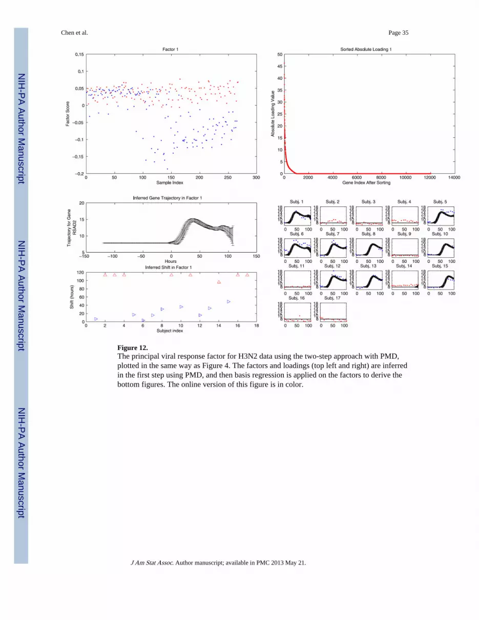
Figure 12.The principal viral response factor for H3N2 data using the two-step approach with PMD,plotted in the same way as Figure 4. The factors and loadings (top left and right) are inferredin the first step using PMD, and then basis regression is applied on the factors to derive thebottom figures. The online version of this figure is in color.
Chen et al. Page 35
J Am Stat Assoc. Author manuscript; available in PMC 2013 May 21.
NIH
-PA Author Manuscript
NIH
-PA Author Manuscript
NIH
-PA Author Manuscript

Figure B.1.The principal viral response factor for the H1N1 data, plotted in the same way as in Figure4. The online version of this figure is in color.
Chen et al. Page 36
J Am Stat Assoc. Author manuscript; available in PMC 2013 May 21.
NIH
-PA Author Manuscript
NIH
-PA Author Manuscript
NIH
-PA Author Manuscript

Figure B.2.The secondary viral response factor for the H1N1 data, plotted in the same way as in Figure6. The online version of this figure is in color.
Chen et al. Page 37
J Am Stat Assoc. Author manuscript; available in PMC 2013 May 21.
NIH
-PA Author Manuscript
NIH
-PA Author Manuscript
NIH
-PA Author Manuscript

Figure B.3.The gender factor for the H1N1 data, plotted in the same way as in Figure 7. The onlineversion of this figure is in color.
Chen et al. Page 38
J Am Stat Assoc. Author manuscript; available in PMC 2013 May 21.
NIH
-PA Author Manuscript
NIH
-PA Author Manuscript
NIH
-PA Author Manuscript
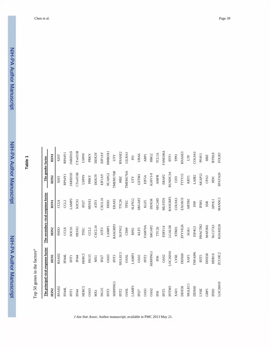
NIH
-PA Author Manuscript
NIH
-PA Author Manuscript
NIH
-PA Author Manuscript
Chen et al. Page 39
Tabl
e 1
Top
50
gene
s in
the
fact
orsa
The
pri
ncip
al v
iral
res
pons
e fa
ctor
The
sec
onda
ry v
iral
res
pons
e fa
ctor
The
gen
der
fact
or
H3N
2H
1N1
H3N
2H
1N1
H3N
2H
1N1
RSA
D2
RSA
D2
IND
OC
CL
8X
IST
XIS
T
IFI4
4LIF
I44L
CC
L8
CC
L2
RPS
4Y1
RPS
4Y1
IFIT
1IF
IT1
SOC
S1L
AM
P3JA
RID
1DJA
RID
1D
IFI4
4IF
I44
HE
SX1
SOC
S1C
Yor
f15B
CY
orf1
5B
HE
RC
5H
ER
C5
TFE
CIF
I27
USP
9YU
SP9Y
OA
S3IS
G15
CC
L2
HE
SX1
PRK
YPR
KY
MX
1M
X1
CX
CL
10A
TF3
DD
X3Y
DD
X3Y
ISG
15IF
I27
AT
F3C
XC
L10
EIF
1AY
EIF
1AY
IFIT
3O
AS3
LA
MP3
IND
ON
CA
PG2
HM
BO
X1
SER
PIN
G1
IFIT
3R
ASG
RP3
ER
AP2
TM
EM
176B
UT
Y
IFIT
2SI
GL
EC
1SL
FN12
TT
C26
HB
ZR
NA
SE2
OA
SLO
ASL
CD
69T
FEC
TM
EM
176A
LIL
RA
3
LA
MP3
LA
MP3
RIN
2SL
FN12
UT
YPI
3
IFI2
7O
AS1
KL
F5SR
GA
P2G
STM
3U
BA
6
OA
S1IF
IT2
FAM
70A
KL
F5E
IF5A
AB
P1
OA
S2SE
RPI
NG
1SR
GA
P2D
DX
58IG
HV
3-9
HB
G2
IFI6
IFI6
TT
C26
SEC
24D
AM
FRT
CL
1A
IFIT
5O
AS2
P2R
Y14
ML
STD
1E
RA
P2FA
M10
6A
IFIT
M3
LO
C26
010
LG
AL
S8R
ASG
RP3
RU
ND
C3A
IFIT
1
XA
F1L
Y6E
STB
D1
CO
L9A
3C
FDT
PP2
DD
X58
DD
X60
ZFY
VE
26E
XO
SC9
TT
TY
15R
NA
SE3
SIG
LE
C1
XA
F1SG
K1
AB
TB
2K
RT
1L
TF
DD
X60
TN
FAIP
6E
IF4G
3D
SPL
AIR
2C
OL
9A3
LY
6EIF
IT5
PHA
CT
R2
IFIH
1A
KA
P12
PF4V
1
GB
P1D
DX
58M
AP2
K6
SSB
CPA
3H
BZ
IFIH
1H
ER
C6
SLC
27A
3A
POL
1H
DC
BT
NL
8
LO
C26
010
ZC
CH
C2
KIA
A02
26M
AN
SC1
SPA
TA
20FO
LR
3
J Am Stat Assoc. Author manuscript; available in PMC 2013 May 21.

NIH
-PA Author Manuscript
NIH
-PA Author Manuscript
NIH
-PA Author Manuscript
Chen et al. Page 40
The
pri
ncip
al v
iral
res
pons
e fa
ctor
The
sec
onda
ry v
iral
res
pons
e fa
ctor
The
gen
der
fact
or
H3N
2H
1N1
H3N
2H
1N1
H3N
2H
1N1
ZC
CH
C2
PLSC
R1
SEC
24D
CE
AC
AM
1H
LA
-DQ
B1
HL
A-D
QB
1
EIF
2AK
2PA
RP1
2C
D16
3T
RIM
5G
PR17
7K
AN
K1
LA
P3R
TP4
AB
TB
2SG
K1
PRK
XC
HI3
L2
IFI3
5IF
ITM
3D
ISC
1A
POL
6PR
SS21
LE
PRO
T
IRF7
ZB
P1C
5SE
RPI
NB
9A
BP1
DE
FA4
PLSC
R1
IFI3
5SC
AR
B2
EIF
4G3
GST
M4
TM
EM
176A
M97
935_
MA
_at
EIF
2AK
2N
OD
1G
NL
YC
LE
C5A
CL
C
RT
P4L
AP3
TM
EM
62IS
G20
S100
A12
VN
N1
M97
935_
MB
_at
IFIH
1D
NA
JC15
C5
KA
NK
1C
YP2
6B1
HE
RC
6M
T2A
ML
STD
1T
RIB
2PY
RO
XD
1FC
GR
2B
TN
FAIP
6IR
F7M
IA3
FLJ2
0699
TG
M3
TM
EM
158
PAR
P12
TO
R1B
SLC
25A
28FA
NC
AG
AT
A2
CD
9
M97
935_
5_at
MX
2K
IAA
0319
LT
RA
FD1
AC
TA
2PL
VA
P
SCO
2D
HX
58C
H25
HD
HX
58C
15or
f29
IL18
RA
P
ZB
P1G
BP1
LO
C93
349
KIA
A03
19L
MA
KA
ZU
1
STA
T1
TIM
M10
TC
F4PH
LPP
MA
D1L
1E
RA
P1
UB
E2L
6SC
O2
RA
BG
AP1
LIG
SF2
LIL
RA
3A
DA
M17
MX
2E
TV
7T
RIB
2T
ME
M62
C21
orf7
C4B
PA
TO
R1B
SAM
D9
HSP
A1B
AB
CG
1E
IF1A
XIG
KV
1-37
M97
935_
3_at
TN
FSF1
0G
OR
ASP
1SC
AR
B2
OA
S1FC
ER
2
TN
FSF1
0M
9793
5_M
A_a
tFL
J206
99FA
M70
AR
NA
SE6
CR
2
TR
IM22
TD
RD
7PH
LPP
TSP
AN
2A
CP5
CY
BR
D1
APO
L6
TR
IM22
UB
A7
RIF
1E
MR
2PV
RL
2
a The
gen
es a
re s
orte
d ac
cord
ing
to th
e ab
solu
te lo
adin
g va
lues
, fro
m m
ost i
mpo
rtan
t to
leas
t im
port
ant.
J Am Stat Assoc. Author manuscript; available in PMC 2013 May 21.


