Group FiveCHAPTER SIX

UCWR

Msc. Cources 2013/2014

1st semester

STEADY GRADUALLY VARIED FLOW

PROF. Abbas Abd. Ibrahim

1

Presented by:

ENG. Lubna Salaheldin Orsud

ENG. Dalal Siddig

Contents

introduction

6.1. Main Problems6.2 Main Objectives

6.3. Main applications in Life6.4. Most Important figures

6.5 Most Important Equations

6.6 Most Important Examples

2

Introduction Gradually varied flow is the steady flow whose depth varied gradually along the length of the channel.A steady non-uniform flow in a prismatic channelwith gradual changes in its water- surface elevation is named as gradually-varied flow (GVF). In a GVF, the Velocity varies along the channel and consequently the bed slope, water surface slope, and energy line slope will all differ from each other. Regions of high curvature are excluded in the analysis of this flow.

6.1 Main ProblemThe streamlines in rapidly varied freesurface flows have considerable curvaturesand slopes; these cause a departure from

3

hydrostatic pressure and uniform velocitydistributions.

6.2 Main Objective This chapter is limited of calculating

rigid boundary, steady-flow, water-surface profiles, , model development

To control the over flow in dams and nature such as floods case. For analytical studies

To find the most design of economical section

Apply hydraulic and hydrological methods to applications in an integrated way

6.3 Main applications in Life1. The backwater produced by a dam or weir across a river and drawdown produced at a sudden drop in a channel are few typical examples of GVF.

2. In engineering practice, trans- critical flow over hydraulic structures such as spillway and weirs are examples of the steady gradually varied flow.

4

3. Application of unsteady flow: Flood routing.

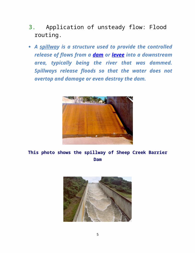
A spillway is a structure used to provide the controlledrelease of flows from a dam or levee into a downstreamarea, typically being the river that was dammed.Spillways release floods so that the water does notovertop and damage or even destroy the dam.

This photo shows the spillway of Sheep Creek BarrierDam

5

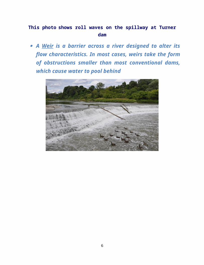
This photo shows roll waves on the spillway at Turnerdam

A Weir is a barrier across a river designed to alter itsflow characteristics. In most cases, weirs take the formof obstructions smaller than most conventional dams,which cause water to pool behind

6

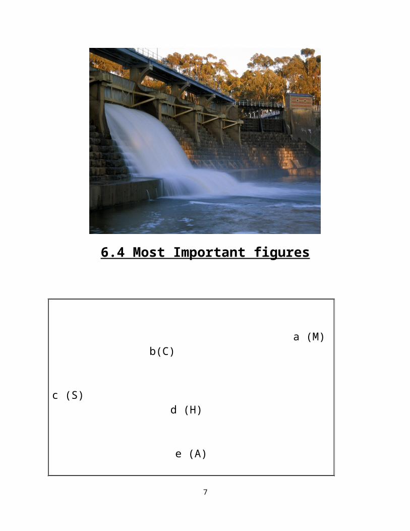
6.4 Most Important figures

7

a (M)b(C)

c (S)d (H)

e (A)

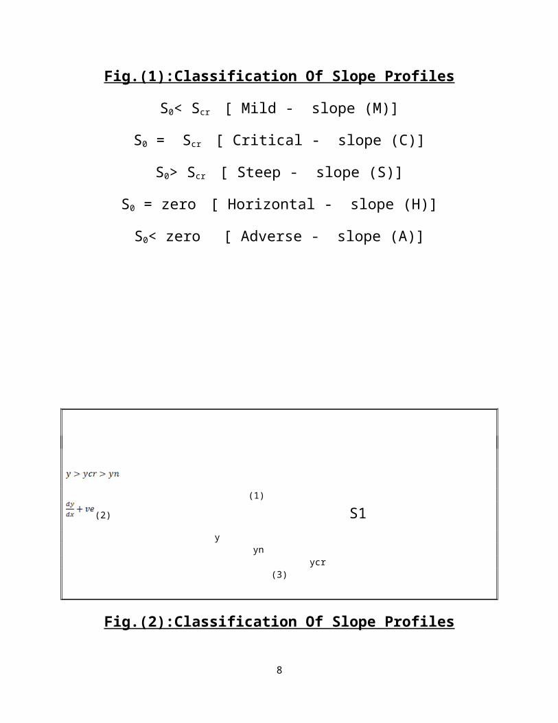
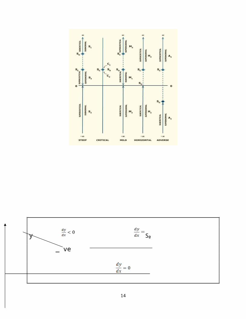
Fig.(1):Classification Of Slope Profiles

S0< Scr [ Mild - slope (M)]

S0 = Scr [ Critical - slope (C)]

S0> Scr [ Steep - slope (S)]

S0 = zero [ Horizontal - slope (H)]

S0< zero [ Adverse - slope (A)]

(1)

(2) S1y

ynycr

(3)

Fig.(2):Classification Of Slope Profiles

8

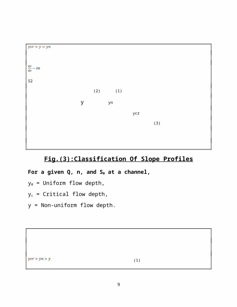
S2

(2) (1)

y yn

ycr

(3)

Fig.( 3 ):Classification Of Slope Profiles

For a given Q, n, and S0 at a channel,

y0 = Uniform flow depth,

yc = Critical flow depth,

y = Non-uniform flow depth.

(1)

9

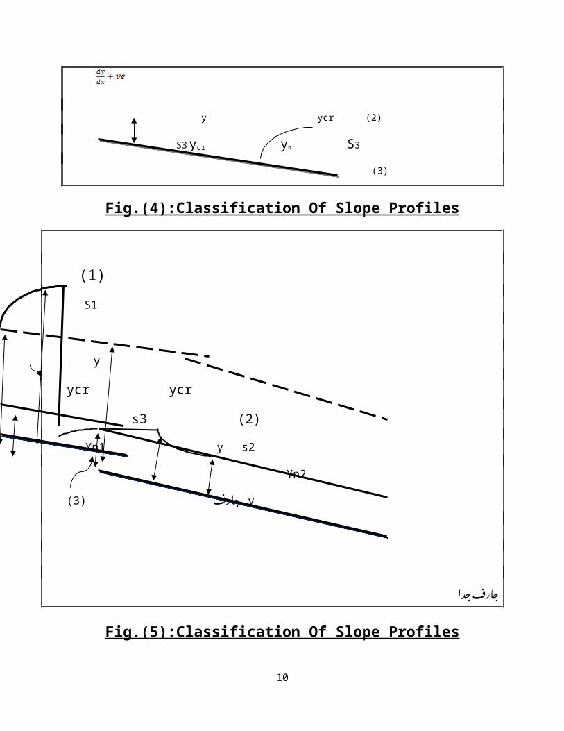
y ycr (2)

S3ycr yn S3(3)

Fig.( 4 ):Classification Of Slope Profiles

(1) S1

y

ycr ycr

s3 (2)

Yn1 y s2

Yn2

ارف� (3) y ج��

دا ارف� ج�� ج��Fig.( 5 ):Classification Of Slope Profiles

10

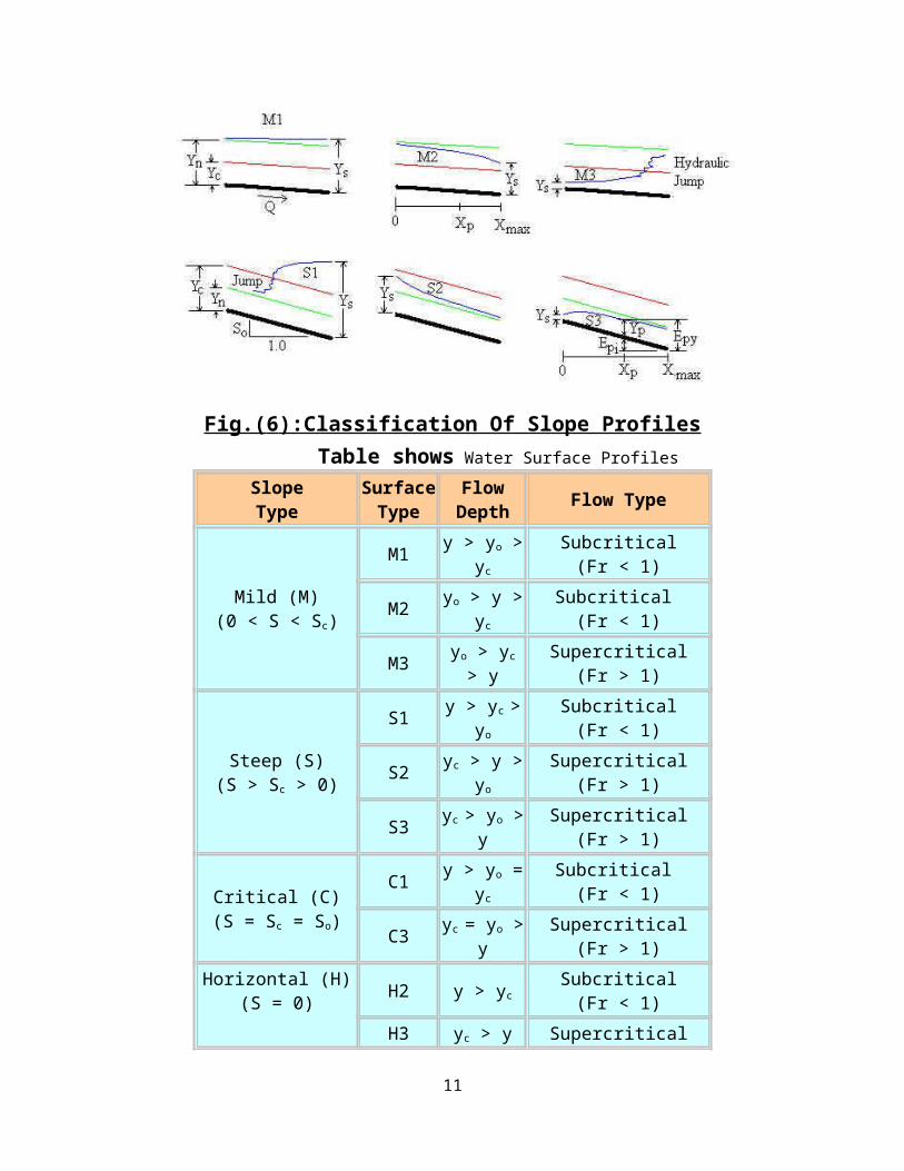
Fig.( 6 ):Classification Of Slope Profiles Table shows Water Surface Profiles

SlopeType

SurfaceType

FlowDepth Flow Type

Mild (M)(0 < S < Sc)

M1 y > yo >yc

Subcritical(Fr < 1)

M2 yo > y >yc

Subcritical (Fr < 1)

M3 yo > yc

> y Supercritical

(Fr > 1)

Steep (S)(S > Sc > 0)

S1 y > yc >yo

Subcritical(Fr < 1)

S2 yc > y >yo

Supercritical(Fr > 1)

S3 yc > yo >y

Supercritical(Fr > 1)

Critical (C)(S = Sc = So)

C1 y > yo =yc

Subcritical (Fr < 1)

C3 yc = yo >y

Supercritical(Fr > 1)

Horizontal (H)(S = 0) H2 y > yc

Subcritical(Fr < 1)

H3 yc > y Supercritical

11

(Fr > 1)

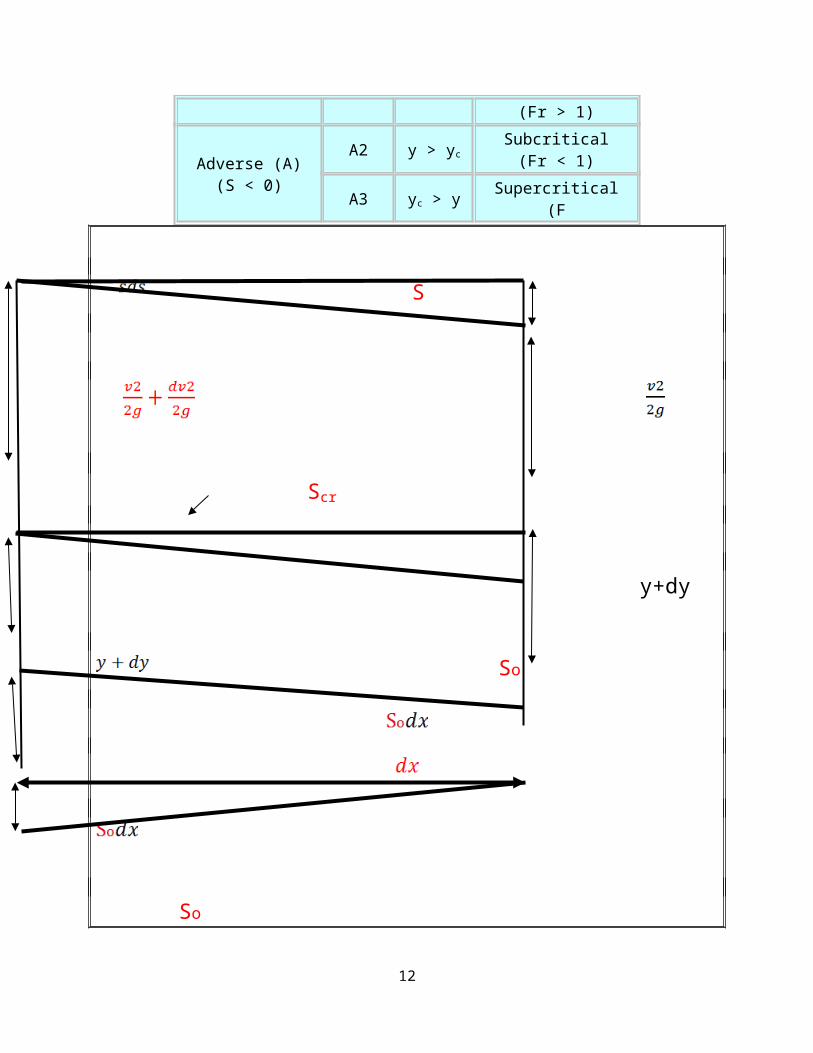
Adverse (A)(S < 0)

A2 y > ycSubcritical(Fr < 1)

A3 yc > y Supercritical(F

S

Scr

y+dy

So

So

12

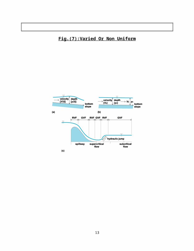
Fig.(7):Varied Or Non Uniform

13

y S0

_ ve

14

+ve

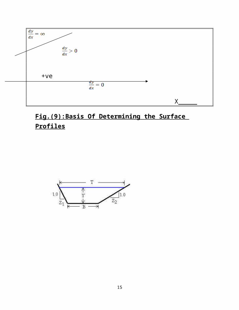
X Fig.(9):Basis Of Determining the Surface Profiles

15

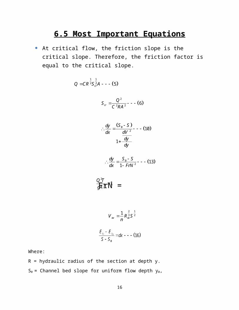
6.5 Most Important Equations At critical flow, the friction slope is the

critical slope. Therefore, the friction factor is equal to the critical slope.

FrN =

Where:

R = hydraulic radius of the section at depth y.

S0 = Channel bed slope for uniform flow depth y0,

16

2

2 2 6crQS

C RA

02 131

S Sdydx FrN

2 13 21

av avV R Sn

02 10

1

S SdydVdxdydy

1 12 2 5crQ CR S A

2

3 1Q TgA

dy = Water depth variation for the dx canal reach,

d (V2/2g) = Velocity head variation for the dx reach.

Q = The discharge

V = The average velocity

Y = The depth of flow

n = The roughness coefficient

S = The normal slope of the canal

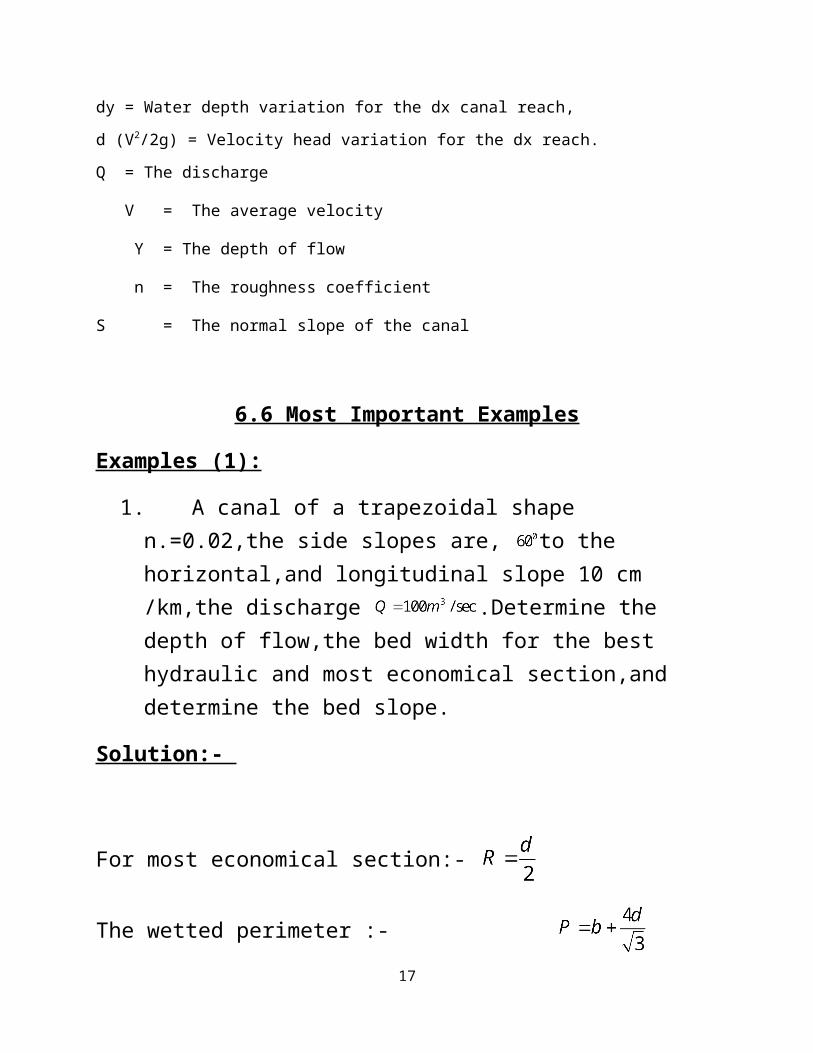
6.6 Most Important Examples

Examples (1):

1. A canal of a trapezoidal shape n.=0.02,the side slopes are, to the horizontal,and longitudinal slope 10 cm /km,the discharge .Determine the depth of flow,the bed width for the best hydraulic and most economical section,and determine the bed slope.

Solution:-

For most economical section:-

The wetted perimeter :-

17

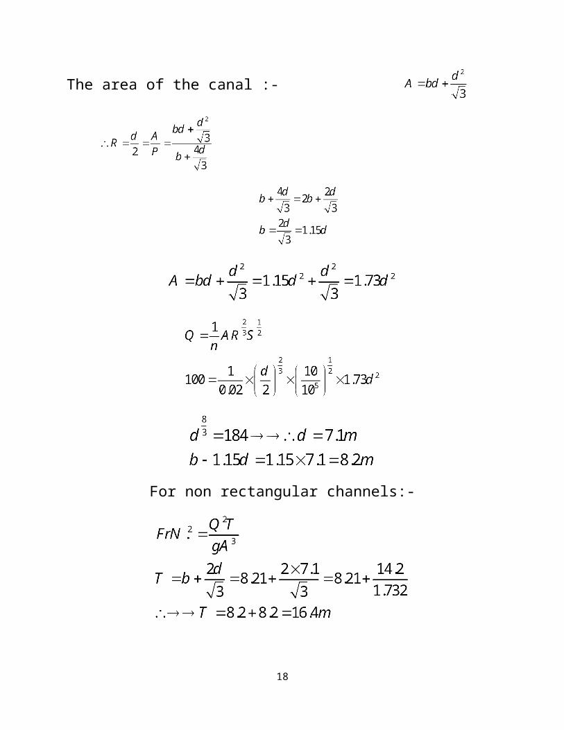
The area of the canal :-

For non rectangular channels:-

18

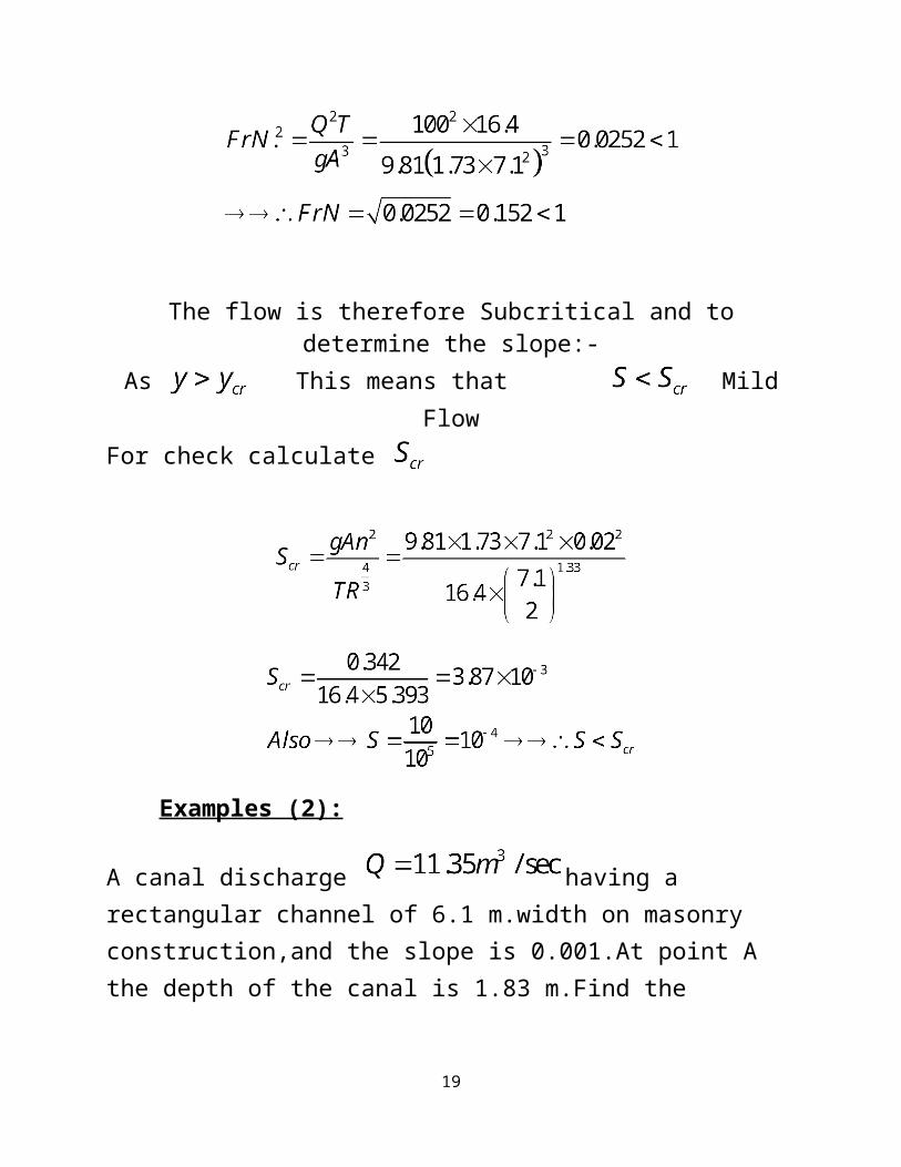
The flow is therefore Subcritical and todetermine the slope:-

As This means that MildFlow

For check calculate

Examples (2):

A canal discharge having a rectangular channel of 6.1 m.width on masonry construction,and the slope is 0.001.At point A the depth of the canal is 1.83 m.Find the

19

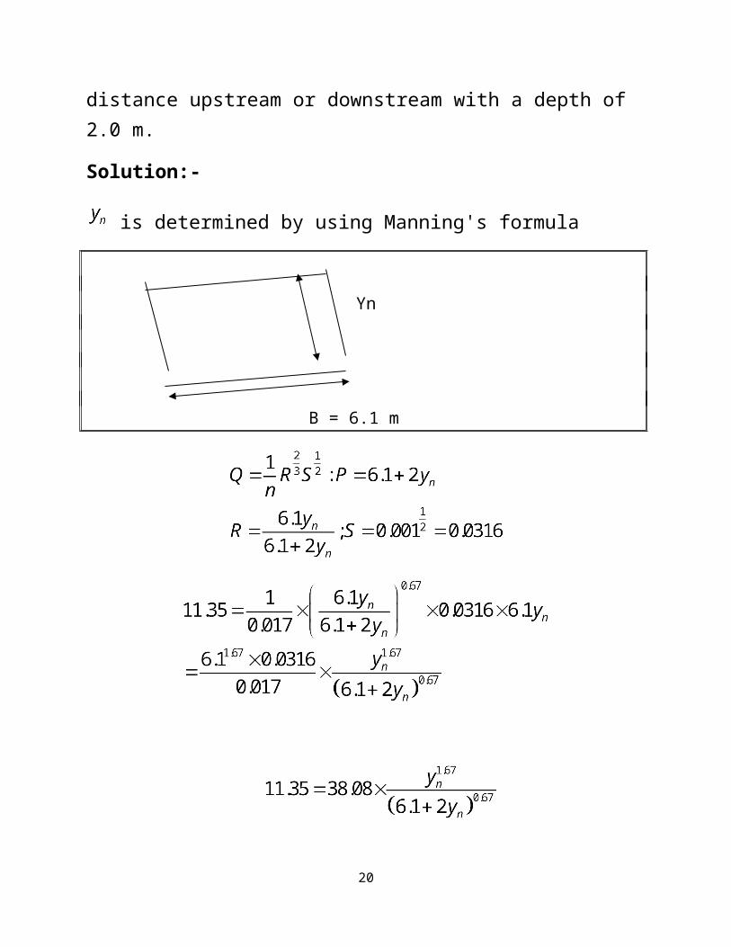
distance upstream or downstream with a depth of 2.0 m.

Solution:-

is determined by using Manning's formula

Yn

B = 6.1 m

20

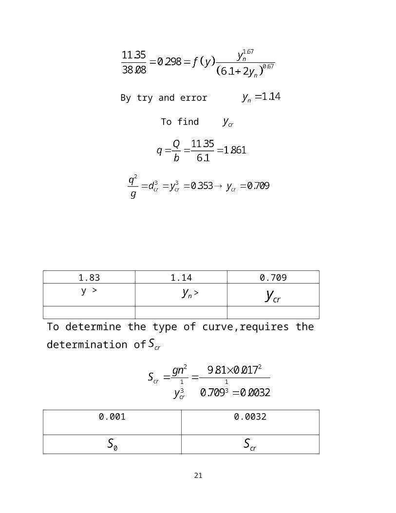
By try and error

To find

1.83 1.14 0.709y > >

To determine the type of curve,requires the determination of

0.001 0.0032

21

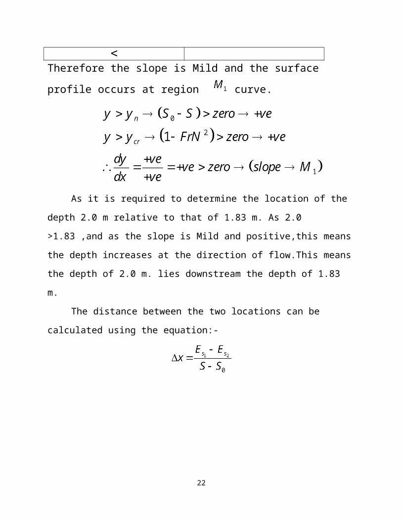
Therefore the slope is Mild and the surface profile occurs at region curve.

As it is required to determine the location of the

depth 2.0 m relative to that of 1.83 m. As 2.0

>1.83 ,and as the slope is Mild and positive,this means

the depth increases at the direction of flow.This means

the depth of 2.0 m. lies downstream the depth of 1.83

m.

The distance between the two locations can be

calculated using the equation:-

22

ك� ان��ت� الا اله لا ال�لهم حان�� �ى س�ب� �ن" م�ن" ك�ن�ت� ان ال�مي% ال�ظ(

23