Embed Size (px)
Citation preview
UNIVERSITE PARIS VII
U.F.R. de Chimie
THESE
présentée à l'Université Paris VII
-p.QUr l"obtention du clipl6me
DE
~AT EN SCIENCES PHYSIQUES
par
Jean-Philippe PUTAUD
LE SULFURE DE DIMETHYLE D'ORIGINE OCEANIQUE:
FLUX, PRODUITS D'OXYDATION ATMOSPHERIQUES ET
INFLUENCE &OR LA. CONCENTRATION DE NOYAUX D'AITIŒN.
Soutenue le 24 Septembre 1993 devant le jury composé de:
MM. G.MOUYŒR Président
O.BRASSSUR J,tapporteur
F.RAB$ Rapporteur
1.C. DUPU!SSV Examinateur
B.C.~ Bxaniinatcur
....
-
UNIVERSITE PARIS VII
U.F.R. de Chimie
THESE
présentée à l'Université
pour l'obtention du
DE
Paris VII
diplôme
DOCTORAT EN SCIENCES PHYSIQUES
par
Jean-Philippe PUTAUD
LE SULFURE DE DIMETHYLE D'ORIGINE OCEANIQUE:
FLUX, PRODUITS D'OXYDATION ATMOSPHERIQUES ET
INFLUENCE SUR LA CONCENTRATION DE NOYAUX D' AITKEN.
Soutenue le 24 Septembre 1993 devant le jury composé de:
MM. G. MOUVIER
G.BRASSEUR
F. RAES
J .C. DUPLESSY
B.C. NGUYEN
Président
Rapporteur
Rapporteur
Examinateur
Examinateur
-
,..
-
Je remercie très sincèrement Monsieur le Professeur G. MOUVIER de la faveur qu'il m'a accordée
en acceptant de présider le jury de cette thèse en ce mois de Septembre 1993.
Je remercie vivement Messieurs G. BRASSEUR et F. RAES pour l'attention qu'ils ont porté à ce
travail et leur participation au jury malgré les dérangements occasionnés par notre éloignement
géographique.
Je remercie également Monsieur B.C. NGUYEN, directeur de cette thèse, pour l'énergie qu'il a
déployée afin de nous permettre d'effectuer nos expériences, pour la confiance qu'il m'a témoignée en
me donnant la responsabilité des mesures effectuées à l'Ile Amsterdam pendant plus d'un an et lors de
deux campagnes océanographiques, pour l'intérêt soutenu qu'il a porté à mon travail ainsi que pour ses
nombreux encouragements à publier les résultats de mes recherches.
Je remercie aussi Monsieur J.-C. DUPLESSY, Directeur du Centre des Faibles Radioactivités, de
m'avoir accueilli dans son laboratoire, d'avoir accepté de participer au jury, et de m'avoir encouragé à
poursuivre ma "carrière" dans la recherche sur le cycle du soufre.
Je tiens aussi à remercier Monsieur Carlo LAJ, Directeur Adjoint du Centre des Faibles
Radioactivités, pour l'intérêt qu'il a porté à mon sujet de recherche et la confiance qu'il m'accordée en
soutenant ma demande de bourse au Commissariat à !'Energie Atomique qui a financé la préparation
de cette thèse.
Un énorme merci à mes deux "grands frères" Sauveur et Nikolas, qui m'ont communiqué leur
enthousiasme pour les recherches que nous poursuivons et transmis leur savoir-faire expérimental,
pour les discussions scientifiques nombreuses et enrichissantes que nous avons eues pendant ces trois
années. Merci aussi à Maria, qui malgré son emploi du temps surchargé, a relu attentivement mon
manuscrit et s'est beaucoup investie pour que je puisse effectuer un "post-doc" intéressant l'année
prochaine. Merci toujours à Hélène qui m'a prêté son matériel de prélèvements d'aérosols pour la
campagne EUMELI 3. Merci encore à Thérèse, Christiane et Stéphanie dont l'efficacité dissout tout
problème administratif dans un sourire.
Un immense merci au Territoire de Terres Austales et Antarctiques Françaises, qui m'a permis
d'effectuer des expériences extraordinaires au cours de séjours inoubliables. Merci à Monsieur B.
DUBOYS pour son soutien, à Bénédicte pour son aide précieuse dans la préparation des missions et les
mesures du radon, à Laurent GALLET et Philippe LAHOZ pour l'analyse d'échantillons d'eau de
pluie d'Amsterdam, au Capitaine et à l'équipage de !'Austral qui m'ont sympathiquement accueilli à
leur bord au cours de trois voyages, et à tous les copains rencontrés dans les TAAF qui ont contribué à ce
que mes séjours là-bas ne m'aient jamais semblé assez longs.
Un très grand merci enfin aux CNRS, INSU, et IFREMER, qui m'ont permis d'effectuer deux
campagnes océanographiques riches d'enseignements, ainsi qu'aux équipages de !'Atalante et du
Suroit pour leur coopération toujours efficace et sympathique.
Table des Matières
Introduction 3
Chapitre I: Le flux océan-atmosphère de sulfure de diméthyle. 13
Comparaison de deux méthodes de calcul du flux de sulfure de diméthyle: le modèle 15 d'échanges océan-atmosphère et le modèle de diffusion turbulente.
Assessment of dimethylsulfide air-sea exchange rate. 19 Putaud J.P., Nguyen B.C., and Weill A., Manuscript.
Conclusion 37
Chapitre II: Les produits d'oxydation atmosphérique du sulfure de diméthyle. 41
A. Concentrations atmosphériques de sulfure de diméthyle et de dioxyde de soufre en 51 milieu océanique.
Seasonal variation of atmospheric sulfur dioxide and dimethylsulfide concentrations at Amsterdam Island 53
in the southern Indian Ocean. Putaud J.P., Mihalopoulos N., Nguyen B.C., Campin J.M., and Belviso S.
Journal of Atmospheric ChemisLry, 15, 117-131. 1992
B. Concentrations et flux de sulfure de diméthyle et d'acide méthanesulfonique en 69 milieu océanique.
Seasonal variation of methanesulfonic acid in precipitation at Amsterdam Island in the southem Indian 71 ocean. Mihalopoulos N., Putaud J.P., and Nguyen B.C., Atmospheric Environment, in press .
C. Impact des produits d'oxydation du sulfure de diméthyle sur l'acidité naturelle des 77 précipitations en milieu océanique.
Covariations of atmospheric dimethylsulfide, its oxydation products and rain acidity at Amsterdam 79
Island in the southern Indian Ocean. Nguyen B.C., Mihalopoulos N., Putaud J.P., Gaudry A., Gallet L., Keene W.C., and Galloway J.N.
Journal of Atmospheric Chemistry. 15, 39-53, 1992.
Conclusion 95
Chapitre III: Sulfure de diméthyle, aérosols et noyaux de condensation. 97
Influence des émissions de sulfure de diméthyle et des composés soufrés particulaires 99 sur la population de noyaux de condensation.
Dimethylsulfide, aerosols and condensation nuclei over the tropical northeastem Atlantic ocean. 103 Putaud J.P., Belviso S., Nguyen B.C., and Mihalopoulos N., Journal of Geophysical Research, in press.
Conclusion 113
Conclusion générale 115
Références bibliographiques 121

Annexes
Annexe I: Le cycle biogéochirnique du soufre.
Article rédigé par J.P. Putaud et B.C. Nguyen pour un ouvrage de géochimie édité par R. Hagemann, J. Jouzel, M. Treuil et L. Turpin.
Annexe II: Techniques d'analyse par chromatographie ionique.
Annexe III: Méthode de mesure de la concentration de noyaux d'Aïtken.
127
129
159
169
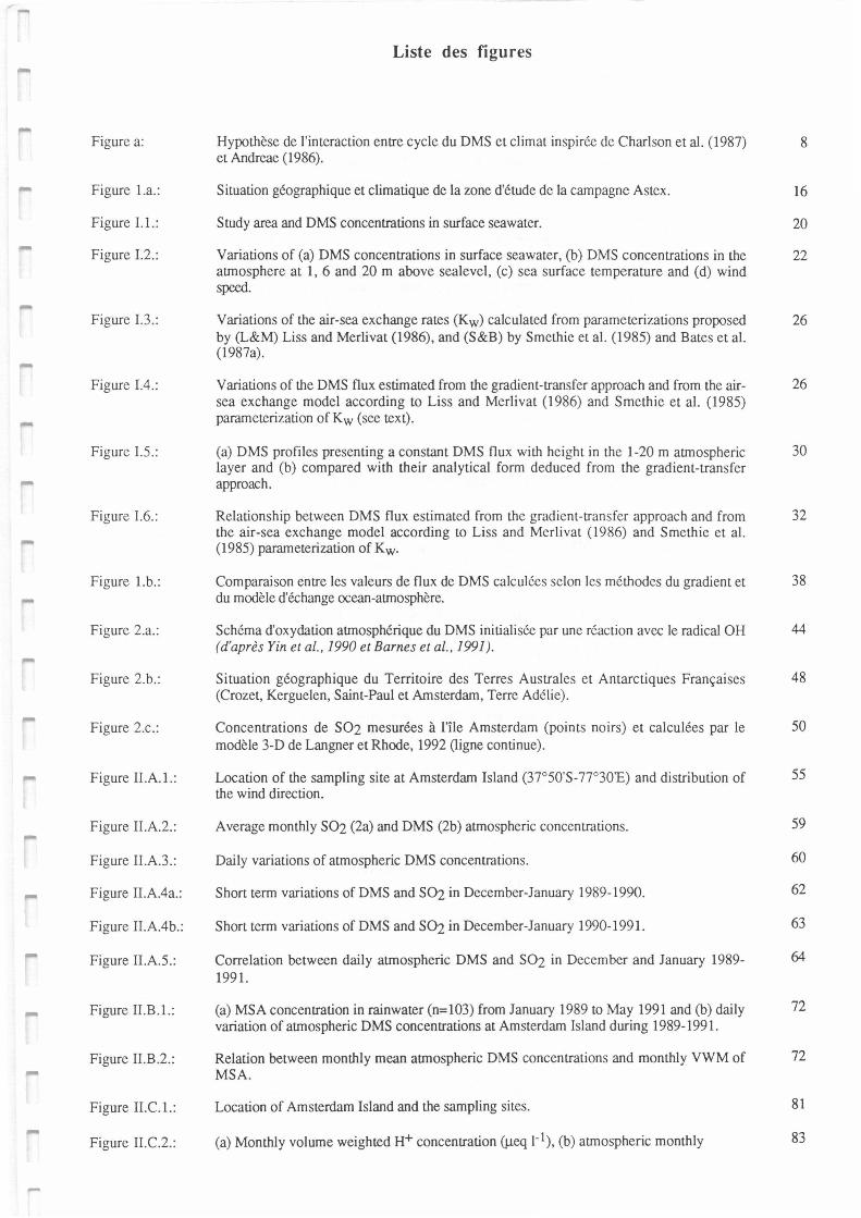
Figure a:
Figure l.a.:
Figure I.l. :
Figure I.2.:
Figure I.3 .:
Figure I.4 .:
Figure I.5.:
Figure I.6. :
Figure l.b.:
Figure 2.a.:
Figure 2.b.:
Figure 2.c.:
Figure II.A. 1.:
Figure II.A.2.:
Figure II.A.3 .:
Figure II.A.4a.:
Figure II.A.4b.:
Figure II.A.5.:
Figure II.B.l. :
Figure II .B.2.:
Figure II.C.1.:
Figure II .C.2.:
-
Liste des figures
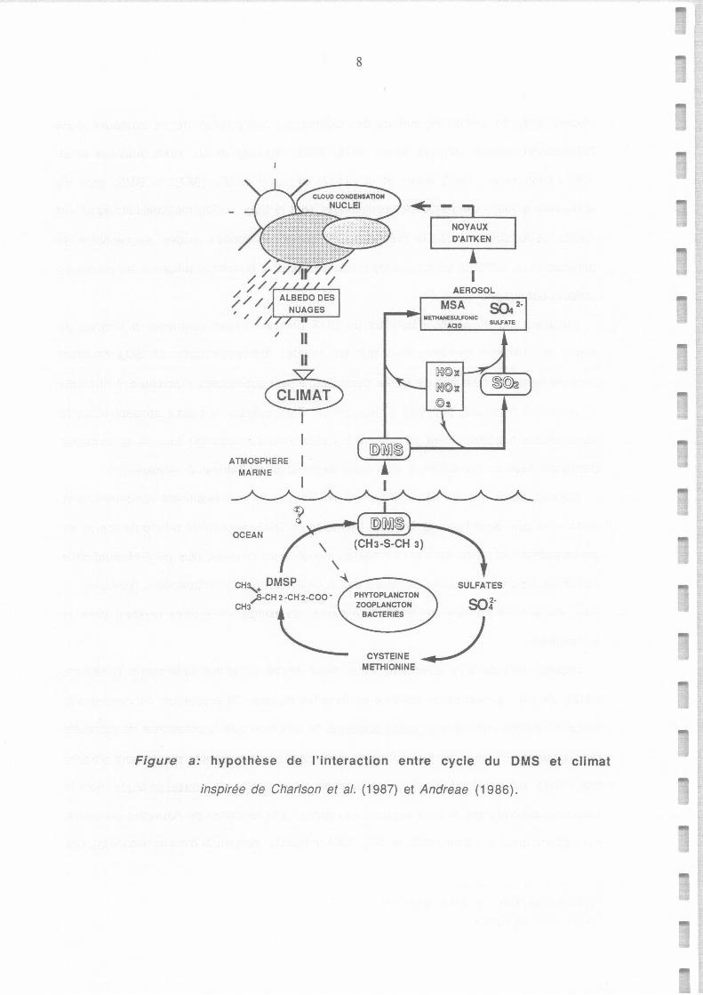
Hypothèse de l'interaction entre cycle du DMS et climat inspirée de Charlson et al. (1987)
et Andreae (1986).
Situation géographique et climatique de la zone d'étude de la campagne Astex.
Study area and DMS concentrations in surface seawater.
Variations of (a) DMS concentrations in surface seawater, (b) DMS concentrations in the
atrnosphere at 1, 6 and 20 m above sealevel, (c) sea surface temperature and (d) wind
speed.
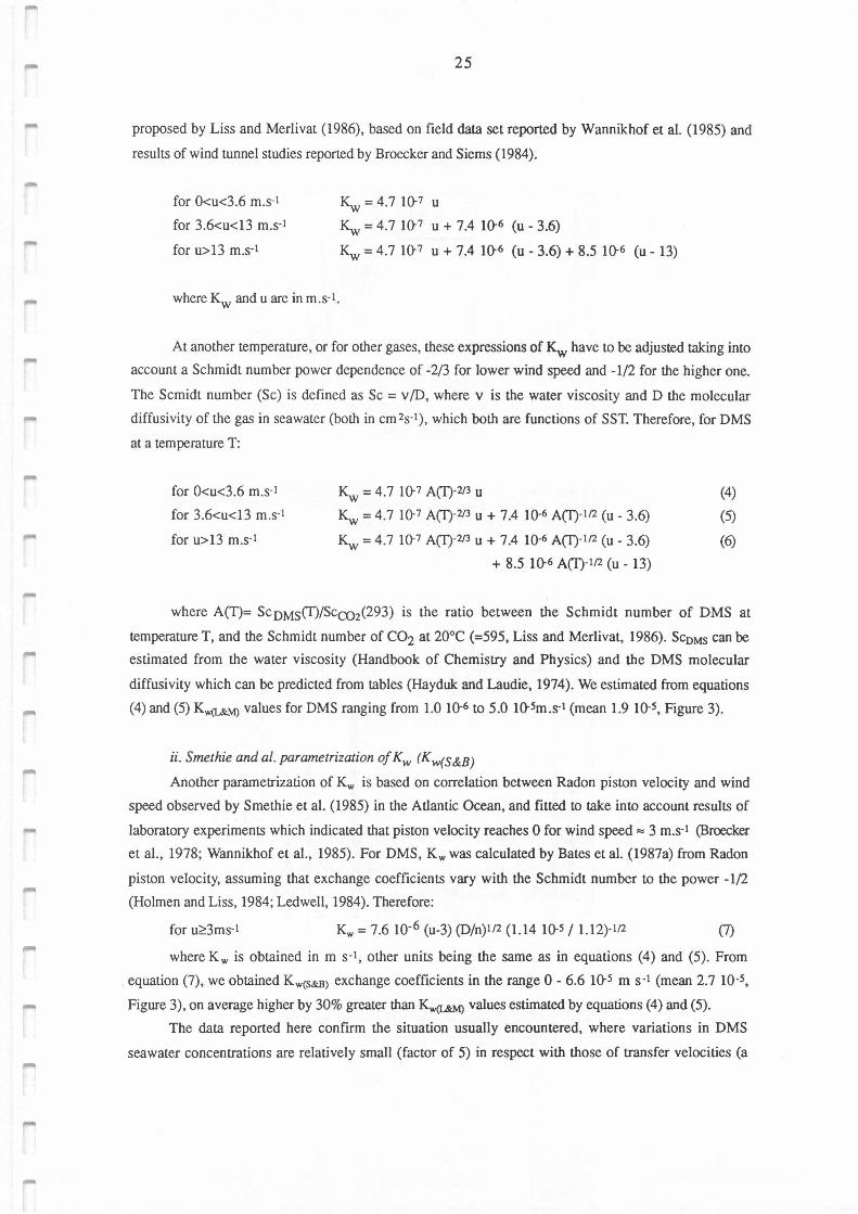
Variations of the air-sea exchange rates (Kw) calculated from parameterizations proposed
by (L&M) Liss and Merlivat (1986), and (S&B) by Smethie et al. (1985) and Bates et al. (1987a).
Variations of the DMS flux estimated from the gradient-transfer approach and from the air
sea exchange mode! according to Liss and Merlivat (1986) and Smethie et al. (1985)
parameterization of Kw (see text).
(a) DMS profiles presenting a constant DMS flux with height in the 1-20 m atrnospheric
layer and (b) compared with their analytical form deduced from the gradient-transfer
approach.
Relationship between DMS flux estimated from the gradicnt-transfer approach and from
the air-sea exchange model according to Liss and Mcrlivat (1986) and Smethie et al.
(1985) parameterization of Kw.
Comparaison entre les valeurs de flux de DMS calculées scion les méthodes du gradient et
du modèle d'échange ocean-atrnosphère.
Schéma d'oxydation atmosphérique du DMS initialisée par une réaction avec le radical OH
(d'après Yin et al., 1990 et Barnes et al., 1991).
Situation géographique du Territoire des Terres Australes et Antarctiques Françaises
(Crozet, Kerguelen, Saint-Paul et Amsterdam, Terre Adélie).
Concentrations de S02 mesurées à l'île Amsterdam (points noirs) et calculées par le
modèle 3-D de Langner et Rhode, 1992 (ligne continue).
Location of the sampling site at Amsterdam Island (37°50'S-77°30'E) and distribution of
the wind direction.
Average monthly S02 (2a) and DMS (2b) atmospheric concentrations.
Daily variations of atmospheric DMS concentrations.
Short term variations of DMS and S02 in December-January 1989-1990.
Short term variations of DMS and S02 in December-January 1990-1991 .
Correlation between daily atmospheric DMS and S02 in December and January 1989-
1991.
(a) MSA concentration in rainwater (n=103) from January 1989 to May 1991 and (b) daily
variation of atrnospheric DMS concentrations at Amsterdam Island during 1989-1991.
Relation between monthly mean atrnospheric DMS concentrations and monthly VWM of
MSA.
Location of Amsterdam Island and the sampling sites.
(a) Monthly volume weighted H+ concentration (µeq 1-1), (b) atrnospheric monthly
8
16
20
22
26
26
30
32
38
44
48
50
55
59
60
62
63
64
72
72
81
83
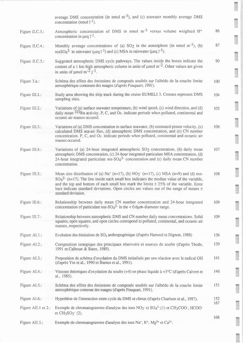
Figure II.C.3. :
Figure II.C.4.:
Figure II.C.5.:
Figure 3.a.:
Figure III.1.:
Figure III.2.:
Figure III.3.:
Figure III.4.:
Figure III.5.:
Figure III.6.:
Figure III.7.:
Figure ALI.:
Figure AI.2.:
Figure AI.3.:
Figure AI.4.:
Figure AI.5.:
Figure AI.6.:
average DMS concentration (in nmol m-3), and (c) seawater monthly average DMS
concentration (nmol 1-1 ).
Atmospheric concentration of DMS in nmol m-3 versus volume weighted H+
concentration in µeq 1-l.
Monthly average concentrations of (a) SO2 in the atmosphere (in nmol m-3), (b)
nssSO42- in rainwater (µeq 1-1) and (c) MSA in rainwater (µeq 1- 1).
Suggested atmospheric DMS cycle pathways. The values inside the boxes indicate the
content of a 1 km high atmospheric column in units of µmol m-2. Other values are given
in units of µmol m·2 j" 1 _
Schéma des effets des émissions de composés soufrés sur l'albédo de la couche limite
atmosphérique contenant des nuages ( d'après Fouquart, 1991 ).
Study area showing the ship track during the cruise EUMELI 3. Crosses represent DMS
sampling sites.
Variations of (a) surface seawater temperature, (b) wind speed, (c) wind direction, and (d)
daily mean 222Rn activity. P, C, and Oc. indicate periods when polluted, continental and
oceanic air masses occured.
Variations of (a) DMS concentration in surface seawater, (b) estimated piston velocity, (c)
calculated DMS sea-air flux, (d) atmospheric DMS concentration, and (e) CN number
concentration. P, C, and Oc. indicate periods when polluted, continental and oceanic air
masses occured.
Variations of (a) 24-hour integrated atmospheric SO2 concentration, (b) daily mean
atmospheric DMS concentration, (c) 24-hour integrated particulate MSA concentration, (d)
24-hour integrated particulate nss-SO4 2- concentration and (e) daily mean CN number
concentration.
Mean size distribution of (a) Na+ (n=17), (b) NO3- (n=17), (c) MSA (n=9) and (d) nss
SO42- (n=17). The line inside each small box indicates the median value of the variable,
and the top and bottom of each small box mark the limits ± 25% of the variable. Error
bars indicate standard deviations. Open circles are values out of the range of means ± standard deviation.
Relationship between daily mean CN number concentration and 24-hour integrated
concentration of particulate nss-SO42- in the< 0.6µm-diameter range.
Relationship between atmospheric DMS and CN number daily mean concentrations. Solid
squares, open squares, and open circles correspond to polluted, continental, and oceanic air
masses, respectively.
Evolution des émissions de SO2 anthropogénique (d'après Hameed et Dignon, 1988)
Composition isotopique des principaux réservoirs et sources de soufre (d'après Thode,
1991 et Calhoun & Bates, 1989).
Proposition de schéma d'oxydation du DMS initialisée par une réaction avec le radical OH
(d'après Yin et al., 1990 et Bames et al., 1991).
Vitesses théoriques d'oxydation du soufre (+4) en phase liquide à +5°C (d'après Calvert et
al., 1985).
Schéma des effets des émissions de composés soufrés sur l'albédo de la couche limite
atmosphérique contenat des nuages (d'après Fouquart, 1991).
Hypothèse de l'interaction entre cycle du DMS et climat (d'après Charlson et al., 1987).
Figure AII.1 et 2.: Exemple de chromatogramme d'analyse des ions NO3- et SOi-.(1) et CH3COO-, HCOO
et CH3SO3- (2).
Figure AII.3.: Exemple de chromatogramme d'analyse des ions Na+, K+, Mg2+ et Ca2+.
86
87
90
100
104
105
106
107
108
109
109
136
139
141
146
151
152
167
168
,...
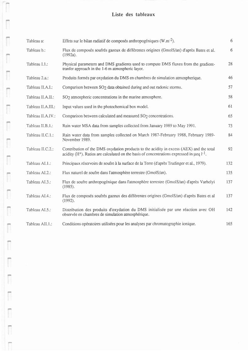
Liste des tableaux
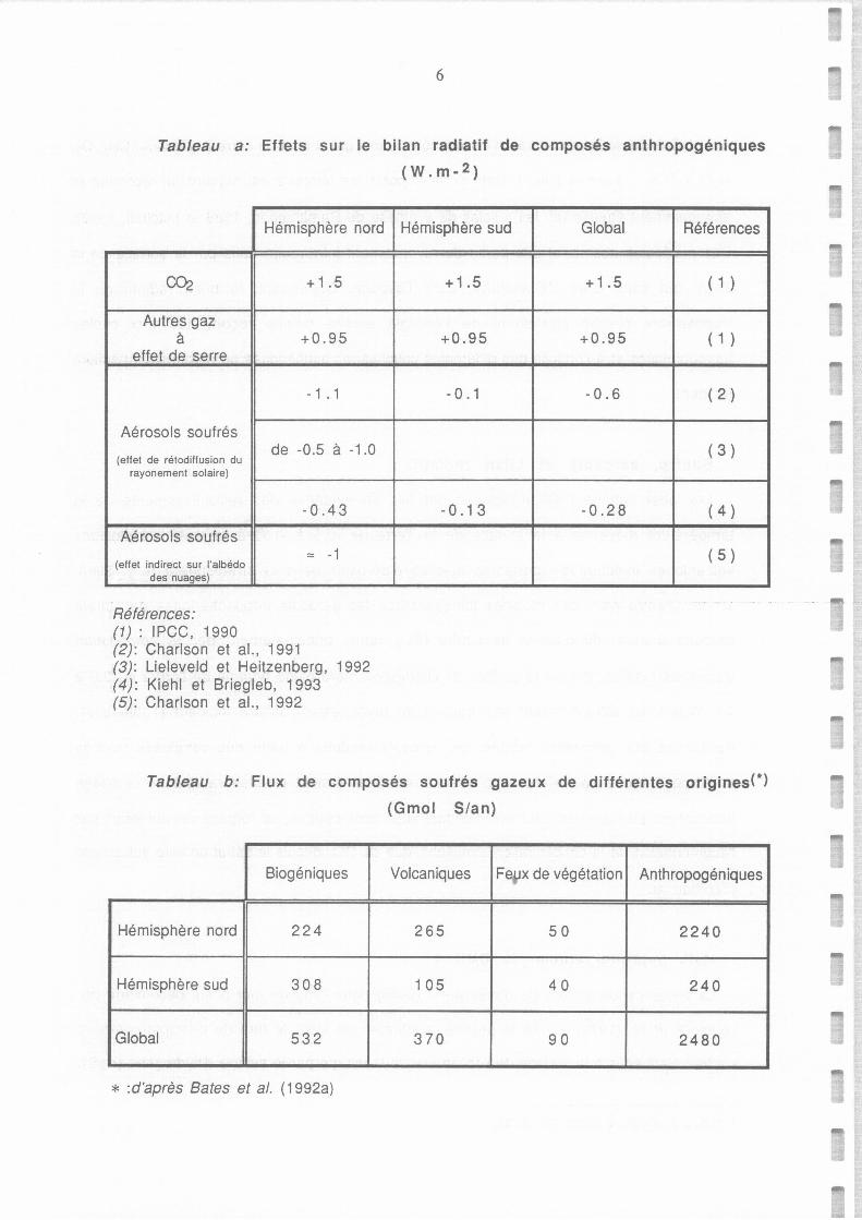
Tableau a: Effets sur le bilan radiatif de composés anthropogéniques (W.m-2). 6
Tableau b.: Flux de composés soufrés gazeux de différentes origines (GmolS/an) d'après Bates et al. 6
(1992a).
Tableau I.1.: Physical parameters and DMS gradients used to compute DMS fluxes from the gradient- 28
tranfer approach in the 1-6 m atmospheric layer.
Tableau 2.a.: Produits formés par oxydation du DMS en chambres de simulation atrnospherique. 46
Tableau 11.A.I.: Comparison between S02 data obtained during and out radonic stonns. 57
Tableau II.A.II.: S02 atmospheric concentrations in the marine atmosphere. 58
Tableau II.A.III.: Input values used in the photochemical box mode!. 61
Tableau II.A.IV.: Comparison between calculated and measured S02 concentrations. 65
Tableau II.B .1.: Rain water MSA data from samples collected from January 1989 to May 1991. 73
Tableau II .C.1.: Rain water data from samples collected on March 1987-February 1988, February 1989- 84
November 1989.
Tableau II.C.2.: Contribution of the DMS oxydation products to the acidity in excess (AEX) and the total 92
acidity (H+). Ratios are calculated on the basis of concentrations expressed in µeq 1-1.
Tableau AI.1.: Principaux réservoirs de soufre à la surface de la Terre (d'après Trudinger et al., 1979). 132
Tableau AI.2.: Flux naturel de soufre dans l'atmosphère terrestre (GmolS/an). 135
Tableau AI.3.: Flux de soufre anthropogénique dans l'atmosphère terrestre (GmolS/an) d'après Varhelyi 137
(1985).
Tableau AI.4.: Flux de composés soufrés gazeux des différentes origines (GmolS/an) d'après Bates et al 137
(1992).
Tableau AI.5.: Distribution des produits d'oxydation du DMS initialisée par une réaction avec OH 142
observée en chambres de simulation atmosphérique.
Tableau Ail.1.: Conditions opératoires utilisées pour les analyses par chromatographie ionique. 165

3
-

-
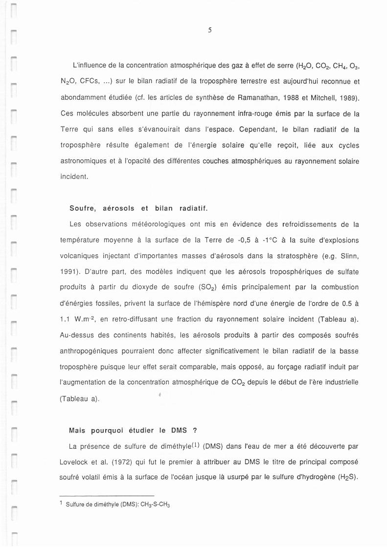
5
L'influence de la concentration atmosphérique des gaz à effet de serre (H2O, CO2 , CH4 , 0 3 ,
N2O, CFCs, ... ) sur le bilan radiatif de la troposphère terrestre est aujourd'hui reconnue et
abondamment étudiée (cf. les articles de synthèse de Ramanathan, 1988 et Mitchell, 1989).
Ces molécules absorbent une partie du rayonnement infra-rouge émis par la surface de la
Terre qui sans elles s'évanouirait dans l'espace. Cependant, le bilan radiatif de la
troposphère résulte également de l'énergie solaire qu'elle reçoit, liée aux cycles
astronomiques et à l'opacité des différentes couches atmosphériques au rayonnement solaire
incident.
Soufre, aérosols et bilan radiatif.
Les observations météorologiques ont mis en évidence des refroidissements de la
température moyenne à la surface de la Terre de -0,5 à -1 °C à la suite d'explosions
volcaniques injectant d'importantes masses d'aérosols dans la stratosphère (e.g. Slinn,
1991 ). D'autre part, des modèles indiquent que les aérosols troposphériques de sulfate
produits à partir du dioxyde de soufre (SO2 ) émis principalement par la combustion
d'énérgies fossiles, privent la surface de l'hémispère nord d'une énergie de l'ordre de 0.5 à
1.1 W.m-2 , en retro-diffusant une fraction du rayonnement solaire incident (Tableau a).
Au-dessus des continents habités, les aérosols produits à partir des composés soufrés
anthropogéniques pourraient donc affecter significativement le bilan radiatif de la basse
troposphère puisque leur effet serait comparable, mais opposé, au forçage radiatif induit par
l'augmentation de la concentration atmosphérique de CO2 depuis le début de l'ère industrielle
(Tableau a).
Mais pourquoi étudier le DMS ?
La présence de sulfure de diméthyle(l) (DMS) dans l'eau de mer a été découverte par
Lovelock et al. (1972) qui fut le premier à attribuer au DMS le titre de principal composé
soufré volatil émis à la surface de l'océan jusque là usurpé par le sulfure d'hydrogène (H2S).
1 Sulfure de diméthyle (OMS) : CH3-S-CH3
6
Tableau a: Effets sur le bilan radiatif de composés anthropogéniques
(W.m- 2 )
Hémisphère nord
00:2 + 1.5
Autres gaz à +0.95
effet de serre
- 1 . 1
Aérosols soufrés de -0.5 à -1.0
(effet de rétodiffusion du rayonement solaire}
-0 .43
Aérosols soufrés == -1
(effet indirect sur l'albédo des nuages}
Références: (1) : IPCC, 1990 (2): Charlson et al., 1991 (3): Lieleveld et Heitzenberg, 1992 (4): Kiehl et Briegleb, 1993 (5): Charlson et al., 1992
Hémisphère sud Global Références
+1.5 +1.5 ( 1 )
+0.95 +0.95 ( 1 )
- 0. 1 -0.6 ( 2 )
( 3 )
-0 .1 3 -0 .2 8 ( 4 )
( 5 )
Tableau b: Flux de composés soufrés gazeux de différentes origines{*)
(Gmol Sian)
Biogéniques Volcaniques Fe.,ix de végétation Anthropogéniques
Hémisphère nord 224 265 50 2240
Hémisphère sud 308 1 05 40 240
Global 532 370 90 2480
* :d'après Bates et al. (1992a)
....
7
Depuis lors, de nombreux auteurs ont discuté de l'importance de ce composé dans
l'atmosphère marine (Nguyen et al., 1978, 1983; Bonsang et al., 1980; Andreae et al.
1983; Toon et al. , 1987, Bates et al., 1987; Charlson et al. , 1987): le DMS, dont les
principaux produits d'oxydation atmosphériques sont le S02, l'acide méthanesulfonique(2J et
l'acide sulfurique(3), serait le précurseur de composés soufrés acides, succeptibles de
participer à la formation de noyaux de condensation, dont le nombre influence les propriétés
optiques des nuages.
Comment les émissions naturelles de DMS pourraient-elles contribuer à l'impact du
soufre sur l'albédo terrestre , alors que les sources antropogéniques de S02 émettent
annuellement des quantités de soufre considérablement supérieures (Tableau b)? Et même
au-dessus des océans, pourquoi s'intéresser au DMS puisque la chimie atmosphérique le
transformera majoritairement en sulfate, introduit dans l'atmosphère lors de la formation
d'embruns avec un flux supérieur d'un ordre de grandeur (cf Tableau 2, Annexe 1) ?
D'abord, parce que les aérosols formés par les sels de mer retombent rapidement à la
surface, et que, dans l'hémisphère sud, l'émission de DMS demeure la principale source de
soufre gazeux. Au moins dans cette moitié du monde, mais peut-être plus généralement dans
toutes les régions océaniques éloignées des sources de pollution importantes, l'émission de
OMS est ainsi à l'origine de la majeure partie des composés soufrés résidant dans la
troposphère .
Ensuite, 95% du S02 anthropogénique serait oxydé en phase hétérogène (Charlson,
1992) , dans les panaches de pollution ou dans les nuages. Ce processus, conduisant à la
formation d'acide sulfurique en phase aqueuse. ne contribue qu'à la croissance de particules
préexistantes. En revanche, l'oxydation du DMS dans une atmosphère propre peut produire
des acides sulfurique (H2S04) et méthanesulfonique (MSA) en phase gazeuse. dont la
nucléation bimoléculaire avec la vapeur d'eau conduit à la formation de nouvelles particules.
Par agglomération et accumulation de S02, MSA et H2S04, mais aussi d'ammoniac (NH3), ces
2 Acide méthane sulfonique (MSA): CH3S03H .
3 Acide sulfurique : H2S04
/ Il
Il
è ATMOSPHERE
MARINE
OCEAN
1
8
•-NOYAUX D'AITKEN
AEROSOL
MSA METHAHE.SULFONIC
AOD
50.2-SULFATE
l}O©i !--'"7.,-.....L--
OO©it
©i
SULFATES
soi·
Figure a: hypothèse de l'interaction entre cycle du DMS et climat
inspirée de Char/son et al. (1987) et Andreae ( 1986).
-
9
particules peuvent croître jusqu'à la taille des noyaux de condensation (CCN),
indispensables à la formation des gouttelettes dans les nuages chauds de basse altitude. Ainsi,
la concentration des produits d'oxydation du DMS peut influencer le nombre de gouttelettes
formées dans desconditions atmosphériques données, et de là les propriétés optiques des
nuages: le OMS dégagé par l'océan aurait donc un effet indirect sur l'albédo de l'atmosphère
terrestre au-dessus des océans.
Enfin, contrairement aux autres sources majeures de soufre, l'émission de DMS à la
surface de l'océan, liée à la sursaturation de l'eau en DMS et à l'efficacité des échanges
océan-atmosphère, est sensible à des paramètres météorologiques. Les échanges océan-
atmosphère sont en effet contrôlés par la vitesse du vent, l'état de la mer et la température
de surface de l'eau. De plus, la production de DMS dans l'eau de mer est le fruit de processus
biologiques complexes. Le DMS est formé dans la couche euphotique des océans par clivage du
diméthylsulfoniopropionate (DMSP(4l). Le DMSP est produit par de nombreuses espèces de
phytoplancton (Keller et al., 1989) et contribuerait à la régulation de la pression osmotique
des cellules (Vairamurthy et al., 1985). Le taux de conversion du DMSP intracellulaire en
DMS semble dépendre du "stress" du phytoplancton: ses phases de sénéscence et de broutage
par le zooplancton conduisent en effet à des concentrations de DMS dissous élevées (Dacey and
Wakeham, 1986; Nguyen et al., 1988; Belviso et al., 1991 ). La dégradation par des
bactéries du DMSP dissous pourrait aussi contribuer à la production de DMS. Il est donc
probable que la concentration de DMS dissous dans l'eau de mer dépende de paramètres
affectant la vie de la poulation planctonique (insolation, température, etc.) .
En conséquence, des variations climatiques, éventuellement dues à l'augmentation de
concentration des gaz à effet de serre, pourraient entraîner une modification du flux de
soufre à la surface des océans qui serait succeptible d 'amplifier ou d'atténuer ces variations.
Cette hypothèse, formulée par Charlson et al. (1987, cf Figure a) , suscite des débats
passionnés dans la communauté scientifique internationale (Bates et al., 1987; Schwartz,
1988; Charlson, 1991 ). En vérité, des incertitudes importantes subsistent quant à la
4 Le diméthylsulfoniopropionate (DMSP) est un zwitterion de formule (CH3)2-s+-(CH2)2-coo-.

10
quantification de nombreuses étapes de la boucle de rétroaction qui lierait l'émission de OMS
océanique et l'albédo de la Terre.
Quelques étapes de la "boucle de Charlson" traitées dans cette thèse:
état des connaissances, questions à résoudre
Ce travail présente des résultats concernant la phase atmosphérique du cycle du OMS,
allant de l'émission de OMS à l'interface océan-atmosphère jusqu'à la formation de noyaux
d'Aïtken (CN).
1. Le flux océan-atmosphère de OMS.
Le flux de OMS n'a jamais été mesuré de manière directe. Classiquement, son estimation
repose sur le modèle d'échange océan-atmosphère proposé par Liss et Slatter (1974), selon
lequel le flux de OMS est proportionnel au gradient de OMS entre l'eau et l'air, et à un
coefficient d'échange dépendant de la température de l'eau, de la vitesse du vent et de l'état de
la mer. Plusieurs paramétrisations de ce coefficient d'échange, basées sur des mesures de
laboratoire et de terrain, ont été proposées (Liss et Merlivat, 1986; Smethie et al., 1985).
Cependant, certains bilans du soufre en milieu océanique ont montré que le flux de soufre qui
se redéposait était sensiblement supérieur au flux de OMS émis à la surface de l'océan
(Nguyen et al., 1992). Ceci pourrait être dû à la sous-estimation des coefficients d'échange,
comme le montre la comparaison entre des flux de C02 calculés à partir de ces
paramétrisations et des mesures de flux de 14C02 (Erickson, 1989).
Le chapitre 1 présente une comparaison entre la méthode classique de calcul du
flux océan-atmosphère de DMS et une méthode s'appuyant sur la théorie de la
diffusion turbulente, selon laquelle le flux d'une variable résulte, dans certaines
conditions, du produit de son gradient atmosphérique par un coefficient de diffusion
turbulent. Cette comparaison est basée sur des mesures simultanées de OMS dans l'eau et
l'atmosphère effectuées au cours d'une campagne océanographique dans l'océan Atlantique, et
11
sur des coefficients d'échange et de diffusion calculés à partir de paramètres physiques
enregistrés au cours de cette campagne. Elle montre une différence (d'un facteur proche de
1.5 à 2 en moyenne) entre les deux méthodes. Les valeurs de flux de DMS présentées dans les
autres chapitres de ce travail ont cependant été calculées selon la méthode classique pour
être comparables avec les résultats publiés dans la littérature.
2. Les produits d'oxydation du OMS en milieu purement océanique.
C'est dans l'hémisphère sud, largement couvert d'océans, que l'impact des composés
soufrés biogéniques sur le climat est potentiellement le plus important. L'évaluation de cet
impact nécessite évidemment une connaissance approfondie des transformations chimiques
subies par le DMS dans l'atmosphère: selon la nature des produits formés (principalement
S02 d'une part, et MSA et H2S04 d'autre part), les processus physiques qui s'ensuivent
peuvent être très différents. Tout comme le S02 anthropogénique, le S02 issu du DMS a
tendance à se solubiliser dans les gouttelettes et le film liquide couvrant les particules pré-
existantes, puis à s'oxyder en phase aqueuse, alors que les acides formés en phase gazeuse
peuvent former de nouvelles particules par nucléation homogène bimoléculaire. La
proportion des différents produits formés par l'oxydation du DMS a été étudiée dans
le chapitre 2 à partir de mesures effectuées à l'ile Amsterdam (Terres Australes et
Antarctiques Françaises), décrivant les variations saisonnières du flux et de la concentration
atmosphérique de DMS, de la concentration atmosphérique de S02, et du flux par dépôt
humide de MSA et de sulfates en excès(5) (nss-S04) . Les concentrations de S02 mesurées ont
été comparées aux résultats d'un modèle de boite photochimique utilisant les concentrations
de DMS mesurées comme données d'entrée et des constantes de vitesse publiées récemment
(Hynes et al., 1986; Atkinson et al., 1989) pour paramétriser la formation et la
destruction du S02. Ceci nous a permis d'évaluer la proportion de DMS oxydée en S02.
Parallèlement, la comparaison du flux de DMS émis par l'océan avec le flux de MSA
5 Dans le terme "sulfates en excès", il faut comprendre sulfate ne provenant pas des embruns marins (non-sea-salt sulfate , nss-S04)
12
retombant dans les précipitations fournit une estimation de la fraction de OMS donnant du
MSA. Enfin, la comparaison des concentrations dans les précipitations des composés MSA(6)
+ nss-S04 et de celle des ions H+ permet d'estimer la contribution des composés soufrés
particulaires à l'acidification des précipitations. Les noyaux de condensation étant
majoritairement formés de composés acides (Twomey, 1971). ceci nous permet de montrer
l'importance des produits d'oxydation du OMS dans la formation des noyaux de condensation.
3. Influence des émissions de OMS et de la concentration de composés soufrés
particulaires sur la population de noyaux de condensation.
Les résultats de mesures effectuées par différents groupes de chercheurs lors de
campagnes océanographiques (Andreae et al., 1993) ainsi qu'à la station de Cape Grim
(Tasmanie) montrent que les variations spatio-temporelles de OMS sont en moyenne
reflétées par les variations de population de CN et CCN (Ayers et al., 1991; Gras, 1990).
Cependant, peu de travaux se sont attachés à étudier les facteurs influençant ces populations
au-dessus des océans de l'hémisphère nord. Cette démarche est entreprise dans le chapitre 3,
dans lequel sont présentées des mesures simultanées des concentrations de composés soufrés
gazeux et particulaires, ainsi que du nombre de noyaux d'Aïtken, effectuées lors d'une
campagne océanographique dans l'Atlantique tropical nord. L'utilisation de traceurs
atmosphériques (activité du Radon et composition de l'aérosol minéral) a permis de
déterminer le caractère des masses d'air échantillonnées qui fut primordial pour
interpréter les variations de OMS et de CN observées.
6 L'utilisation de l'abbréviation MSA (MethaneSulfonic Acid) est ici abusive puisque c'est la concentration de la base conjuguée (l'ion méthanesulfonate) qui est en réalité mesurée.
13
CC IHI A lP IIirIIUE II
LE FLUX OCEAN-ATMOSPHERE DE SULFURE DE DIMETHYLE.

15
LE FLUX OCEAN-ATMOSPHERE DE SULFURE DE DIMETHYLE.
COMPARAISON DE DEUX METHODES DE CALCUL DU FLUX DE SULFURE DE DIMETHYLE:
LE MODELE D'ECHANGE OCEAN-ATMOSPHERE ET LE MODELE DE DIFFUSION TURBULENTE.
Pour quantifier l'effet de l'émission du OMS sur l'albédo de l'atmosphère terrestre et
prévoir les conséquences de variations climatiques futures sur ce taux d'émission, il est
primordial de déterminer la relation liant le flux océan-atmosphère de OMS et les
paramètres dont il dépend. Jusqu'à présent, aucune mesure directe de ce flux n'a été
rapportée. La méthode de boîte consistant à isoler dans une enceinte une fraction de la
surface au travers de laquelle le flux doit être mesuré, habituellement utilisée pour
mesurer les émissions de gaz par les sols, ne peut en effet être employée sur l'eau
puisqu'elle annule localement la vitesse du vent, qui est le moteur des échanges océan-
atmosphère. Une autre méthode (eddy correlation) semble prometteuse mais nécessite des
mesures à hautes fréquences et de grande précision des concentrations de OMS et de la
composante verticale du vent, qui ne sont pas encore totalement réalisables.
Les estimations des flux d'échanges de gaz entre l'océan et l'atmosphère sont donc obtenues
en utilisant un modèle décrit par Liss et Slatter (1974), dans lequel le flux air-mer d'une
espèce gazeuse est calculé par le produit du gradient de concentration de ce gaz entre l'eau et
l'atmosphèreO) par un coefficient d'échange Kw:
F = Kw (Cw·Ca/H)
Des mesures de terrain (Wannikhof et al., 1985; Smethie et al., 1985) et des expériences
effectuées en tunnel (Broecker et Siems, 1984) ont permis de montrer que Kw est lié à la
vitesse du vent et l'état de la mer. Des corrélations ont permis d'estimer ce coefficient pour
des gaz tels que le C02 dont le nombre de Schmidt(2) dans l'eau est proche de
1 Le gradient océan-atmosphère est défini comme t.c = cw - ca!H, où cw est la concentration du composé dans l'eau, ca sa concentration dans l'air et H la constante de Henry (égale à l'inverse de la solubilité) qui dépend du composé, ainsi que de la composition et de la température de l'eau.
2 Le nombbre de Schmidt (Sc) est un nombre sans dimension qui caractérise la "mobilité" de l'espèce qui diffuse. Il est égal au rapport entre la diffusivité du gaz et la viscosité du milieu (Sc = v /0).
4o·w
/ /1 D/
40°N /
/ ,/
0 -1 . '\
. --
< 20 --·
; -· ~
-- _..,. / ~ - ~-:
1._- .
'
16
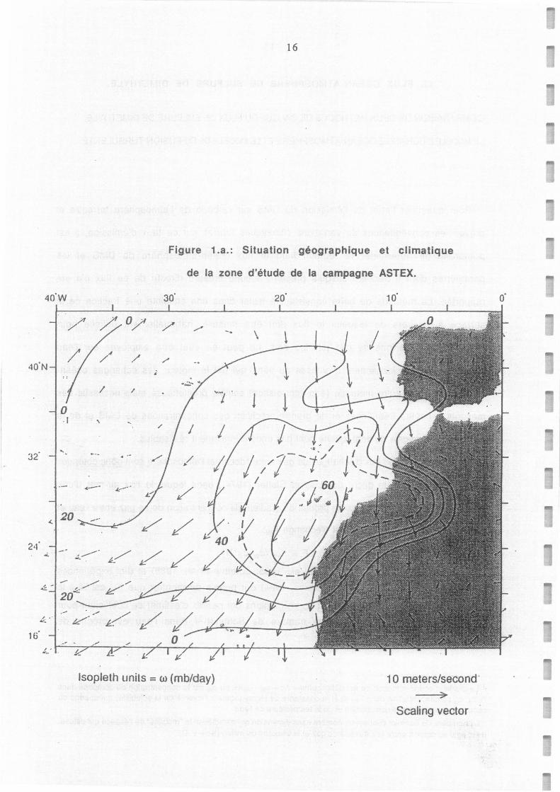
Figure 1.a.: Situation géographique et climatique
de la zone d'étude de la campagne ASTEX.
30· 20·
/ / -~ \ l /
... , l
/
lsopleth units = w (mb/day) 1 O meters/second· ;)
Scaling vector
,....
17
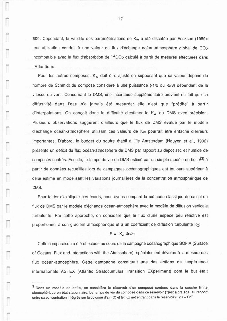
600. Cependant, la validité des paramétrisations de Kw a été discutée par Erickson (1989):
leur utilisation conduit à une valeur du flux d'échange océan-atmosphère global de CO2
incompatible avec le flux d'absorbtion de 14CO2 calculé à partir de mesures effectuées dans
l'Atlantique.
Pour les autres composés, Kw doit être ajusté en supposant que sa valeur dépend du
nombre de Schmidt du composé considéré à une puissance (-1/2 ou -2/3) dépendant de la
vitesse du vent. Concernant le OMS, une incertitude supplémentaire provient du fait que sa
diffusivité dans l'eau n'a jamais été mesurée: elle n'est que "prédite" à partir
d'interpolations. On conçoit donc la difficulté d'estimer le Kw du OMS avec précision.
Plusieurs observations suggèrent d'ailleurs que le flux de OMS évalué par le modèle
d'échange océan-atmosphère utilisant ces valeurs de Kw pourrait être entaché d'erreurs
importantes. D'abord, le budget du soufre établi à l'île Amsterdam (Nguyen et al., 1992)
présente un déficit du flux océan-atmosphère de OMS par rapport au dépot sec et humide de
composés soufrés. Ensuite, le temps de vie du OMS estimé par un simple modèle de boite(3) à
partir de données recueillies lors de campagnes océanographiques est toujours supérieur à
celui estimé en modélisant les variations journalières de la concentration atmosphérique de
OMS.
Pour tenter d'expliquer ces écarts, nous avons comparé la méthode classique de calcul du
flux de OMS par le modèle d'échange océan-atmosphère avec le modèle de diffusion verticale
turbulente. Par cette approche, on considère que le flux d'une espèce peu réactive est
proportionnel à son gradient atmosphérique et à un coefficient de diffusion turbulente K2 :
F = -K2 oc/oz
Cette comparaison a été effectuée au cours de la campagne océanographique SOFIA (Surface
of Oceans: Flux and Interactions with the Atmosphere), spécialement dévolue à la mesure des
flux océan-atmosphère. Cette campagne constituait une des actions de l'expérience
internationale ASTEX (Atlantic Stratocumulus Transition EXperiment) dont le but était
3 Dans un modèle de boîte, on considère le réservoir d'un composé contenu dans la couche limite atmosphérique en état stationnaire. Le temps de vie du composé dans ce réservoir ('t)est alors égal au rapport entre sa concentration intégrée sur la colonne d'air (C) et le flux net entrant dans le réservoir (F): 't = C/F.
18
d'étudier les facteurs influançant la formation et la dissipation des stratocumulus, et
l'impact des aérosols, de la microphysique des nuages et de la chimie atmosphérique sur les
propriétés de ces nuages. La zone d'étude (Océan Atlantique, au sud des Açores, Figure 1.a.)
avait été choisie en raison de sa climatologie indiquant une forte probablilité de rencontrer
une grande variété de nuages dans la couche limite atmosphérique.
L'originalité de cette campagne était que les mesures effectuées à bord du Suroit
permettaient de calculer des valeurs de flux de OMS par les deux méthodes décrites ci-dessus
pour le même endroit et le même instant. Les paramètres météorologiques et le gradient de
concentration de OMS entre l'eau de surface et l'atmosphère conduirent à l'estimation du flux
de OMS par la méthode classique. Parallèlement, les mesures de paramètres physiques
destinés à déterminer les flux de chaleur, humidité et quantité de mouvement, permettraient
de calculer des valeurs instantanées du coefficient de diffusion turbulente, qui associés aux
gradients atmosphériques de OMS mesurés donnaient des estimations du flux de OMS par le
modèle de diffusion turbulente. Les valeurs de flux de OMS obtenues par ces deux méthodes
totalement indépendantes, en utilisant différentes paramétrisations des coefficients Kw
(Smethie et al., 1985; Liss et Merlivat, 1986) et Kz (Businger et al., 1971; Oyer and
Bradley, 1982) sont comparées dans l'article présenté ci-après.
19
ASSESSMENT OF DIMETHYLSULFIDE SEA-AIR EXCHANGE RATE.
J .P. PUTAUD and B.C. NGUYEN
Centre des Faibles Radioactivités, Laboratoire Mixte CNRS-CEA, 91198 Gif-sur-Yvette Cedex, France
A. WEILL
Centre de Recherche en Physique del' Environnement, 10-12 avenue del' Europe, 78140 Vélizy, France.
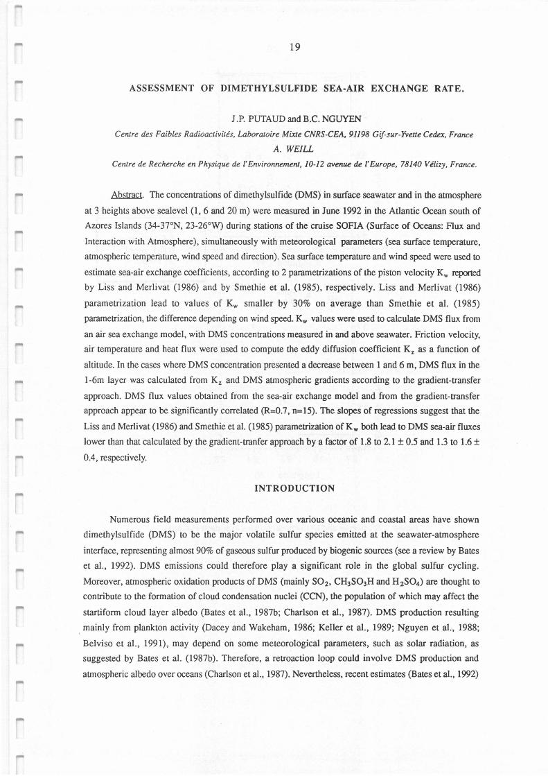
Abstract. The concentrations of dimethylsulfide (DMS) in surface seawater and in the atmosphere
at 3 heights above sealevel (1, 6 and 20 m) were measured in June 1992 in the Atlantic Ocean south of
Azores Islands (34-37°N, 23-26°W) during stations of the cruise SOFIA (Surface of Oceans: Flux and
Interaction with Atmosphere), simultaneously with meteorological parameters (sea surface temperature,
atmospheric temperature, wind speed and direction). Sea surface temperature and wind speed were used to
estimate sea-air exchange coefficients, according to 2 parametrizations of the piston velocity Kw reported
by Liss and Merlivat (1986) and by Smethie et al. (1985), respectively. Liss and Merlivat (1986)
parametrization lead to values of Kw smaller by 30% on average than Smethie et al. (1985)
parametrization, the difference depending on wind speed. Kw values were used to calculate DMS flux from
an air sea exchange mode!, with DMS concentrations measured in and above seawater. Friction velocity,
air temperature and heat flux were used to compute the eddy diffusion coefficient K2 as a fonction of
altitude. In the cases where DMS concentration presented a decrease between 1 and 6 m, DMS flux in the
l-6m layer was calculated from K2 and DMS atmospheric gradients according to the gradient-transfer
approach. DMS flux values obtained from the sea-air exchange mode! and from the gradient-transfer
approach appear to be significantly correlated (R=0.7, n=15). The slopes of regressions suggest that the
Liss and Merlivat (1986) and Smethie et al. (1985) parametrization of Kw both Iead to DMS sea-air fluxes
lower than that calculated by the gradient-tranfer approach by a factor of 1.8 to 2.1 ± 0.5 and 1.3 to 1.6 ±
0.4, respectively.
INTRODUCTION
Numerous field measurements performed over various oceanic and coastal areas have shown
dimethylsulfide (DMS) to be the major volatile sulfur species emitted at the seawater-atmosphere
interface, representing almost 90% of gaseous sulfur produced by biogenic sources (see a review by Bates
et al., 1992). DMS emissions could therefore play a significant role in the global sulfur cycling.
Moreover, atmospheric oxidation products of DMS (mainly SO2, CH3SO3H and H 2SO4) are thought to
contribute to the formation of cloud condensation nuclei (CCN), the population of which may affect the
startiform cloud layer albedo (Bates et al., 1987b; Charlson et al., 1987). DMS production resulting
mainly from plankton activity (Dacey and Wakeham, 1986; Keller et al., 1989; Nguyen et al., 1988;
Belviso et al., 1991), may depend on some meteorological parameters, such as solar radiation, as
suggested by Bates et al. (1987b). Therefore, a retroaction Ioop could involve DMS production and
atmospheric albedo over oceans (Charlson et al., 1987). Nevertheless, recent estimates (Bates et al., 1992)
20
38 Ponta • 1a: Leg 1 Delgada
37 c\o 6>o 0
0 0 0
0 0
36 0 08 0
CD z
%0 °tb ~ 0 Q)
35 0 0 Q
"O 0 :::, (Ç) -:;:; 0 C\1 ..J
0 <0.5 nmol.I-1 34 0 0.5-0.8 nmol.I-1
27 26 25 24 23 0 0.8-1 nmol.I-1
Longitude (0 W) 0 >1 nmol.I-1
• Ponta Delgada
38 • Ponta
c9 Delgada 0
37 0 0
Cb. 0 0
~
• • . 36 oO
0
z 0 0 - oo Q) 35 "O :::, -:;:; C\1 ..J
1b: Leg 2 34
27 26 25 24 23
Longitude (0 W)
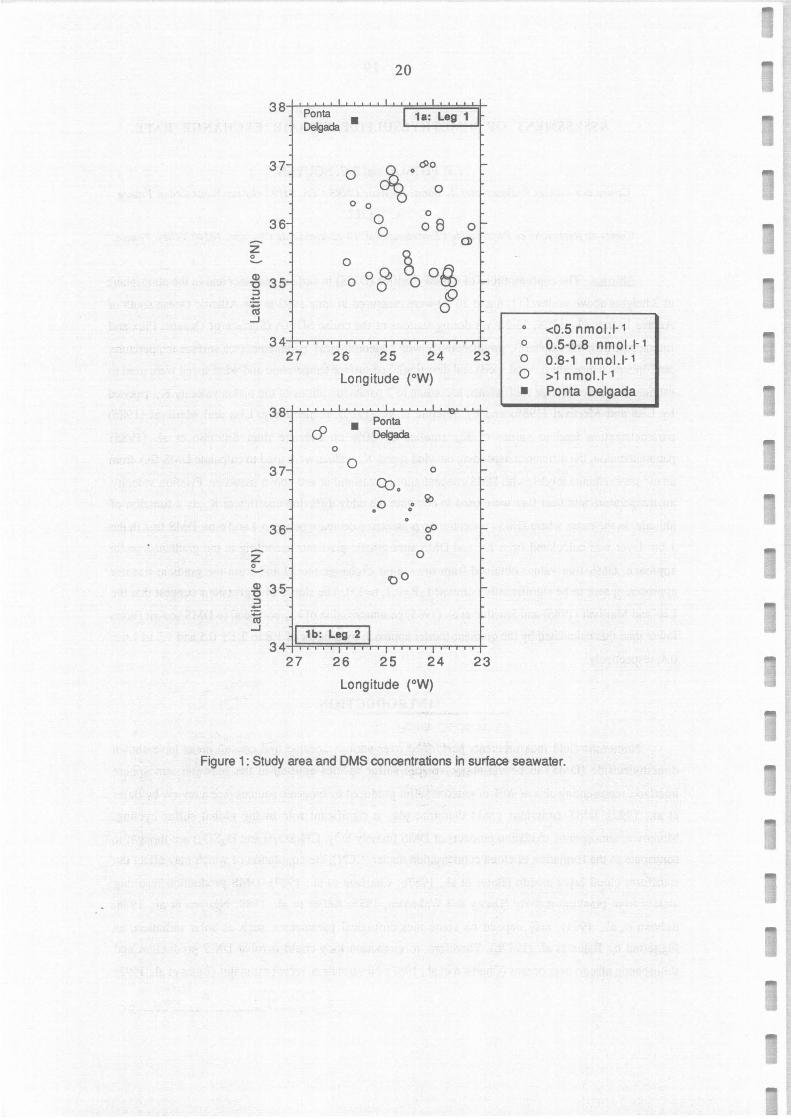
Figure 1: Study area and OMS concentrations in surface seawater.
-
-
21
indicate that anthropogenic emissions of gaseous sulfur (mainly SO2) nowadays largely exceed natural
emissions on a global scale. But uncertainties in estimates of DMS global flux rates still exist (see for
example Andreae, 1986), and refinements in its evaluation are needed to determine DMS potential
climatic impact, at least over oceanic areas and particularly in the southern hemisphere where DMS
emission is still thought to be the principal sulfur source.
The use of the sea-air exchange model described by Liss and Slater (1974) have been the method
classically employed to estimate DMS sea-air flux (see for example Bates, 1987a, 1992; Berresheim,
1987; Andreae et al., 1989; Leck and Rhode, 1991; Nguyen et al., 1990, 1992). In this method, the sea-
air flux is assumed to be equal to the product of an exchange coefficient across the interface by the
concentration gradient between surface seawater and the atmosphere. Attempts to balance local sulfur
budgets by using this method indicate that DMS sea-air fluxes do not match better than by a factor of
about 2 with measured or estimated deposition fluxes of DMS oxidation products (Berresheim, 1987;
Nguyen et al., 1992). Although this kind of budgets is subject to large uncertainties, at least partially due
to long range transport and exchanges of sulfur compounds between troposphere and stratosphere, these
unbalances suggest that the uncertainty on DMS sea-air flux estimates could be a factor of 2, mainly due
to uncertainties in the sea-air exchange coefficients. A similar result have been obtained by Erickson
(1989) who found that the exchange coefficient detennined from Liss and Merlivat (1986) parametrization
had to be multiplied by a factor of 1.8 to be consistent with measurements of 14CO2 exchange rates.
In this paper, 2 different parametrizations of exchange coefficients are used to estimate DMS sea-
air flux by an sea-air exchange model based on simultaneous DMS and meteorological parameters
measurements performed in the Atlantic ocean. These estimates are compared with DMS flux values
calculated by using the gradient-transfer approach, based on eddy diffusion coefficient computed from
meteorological parameters and atrnospheric DMS gradients in the 1-20m layer. Comparison between these
two independant methods is investigated to assess estimate of DMS ocean-to-atmosphere flux.
EXPERIMENTAL
Surface seawater and atmospheric samples were collected in June 1992 on board R/V Le Suroit
during SOFIA (Surface of Oceans: Flux and Interactions with the Atrnosphere) experiment in the south of
Sao Miguel Island (Azores), between 34°N and 38°N, and 23°W and 27°W (Figure 1). About 60 ml of
surface seawater were sampled every 6 hours (0, 6, 12 and 18hr local time) from the bucket devoted to sea
suface temperature (SST) measurements, using a polypropylene syringe. The seawater samples were
immediately injected into a bubbler, where DMS was extracted by helium bubbling at a flow rate of 100
mVmin and concentrated in a cryogenic trap at -90°C before being analysed by GC/FPD [Nguyen et al.,
1990]. The accuracy of the analysis is estimated to be about 10%.
Atmospheric samples were simultaneously collected at 1 and 6m above sealevel, 3 meters in front
of the bow of the ship, and at 20 m above sealevel from the signal mast, only when the ship was heading
into the wind, with a velocity smaller than 2 knt. It should be noted that these sampling conditions do
not totally exclude risks of atmospheric profiles disturbance by the ship. About 25 1 of air were collected
2
-,_
0 E C:
i ffi Q) ., .!:
~ 0
0
'? 4 E
-"! .§.
l ,:, C:
~
0 E .:.3
~ .g 2 Q)
1 E 1 <
14 1 2 10
8
6 4 2 0
(') Il)
(') Il)
22
I'- "' (') Il) I'- "'
Day (June 1992)
----+--20m
Day (June 1992)
Day (June 1992)
2d
~ I'- "'
(') Il) I'- "' Day (June 1992)
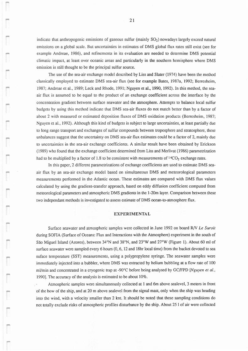
Figure 2: Variations of (a) OMS concentrations in surface seawater, (b) OMS concentrations in the atmosphere at 1,6, and 20 m above sealevel, (c) sea surface temperature and (d) wind speed.
,..
,...
,..
-
23
twice a day when possible, once before the sunrise, and once around noon. On the total, 29 vertical
profiles of DMS concentrations were measured. The analysis of the air samples was performed within 3
hours after sampling, using the same method as for seawater samples [Nguyen et al., 1990]. The
detection limit was about 0.4 nmol m -3 for this experiment. The accuracy of the analysis is estimated to
be about 10%, and several tests performed on board indicated that the standard deviation on 3 analyses of
the same sample was Jess than 3%.
SST was measured every 3 hours using a standard bucket to sarnple seawater, with an accuracy of
±0.1 °C. Comparing to other SST measurements performed on board, a possible bias of Iess than 0.3°C
has been estimated, which does not imply a large uncertainty in fluxes and drag coefficients, taking into
account the low wind speed observed during the experiment (Figure 2d). Wind speed and air temperature
were measured by a POMMAR station at 15 m above sealevel, with an accuracy of ±0.5m.s-l and
±0.1°C, respectively. These data were used to determine friction velocity (u*) and surface virtual flux
temperature (<w' 0'>) using bulk parametrizations (Large et Pond, 1982; Klaptsov, 1983). These <w' 0'>
values were not different by more than 20% compared with inertial dissipative method (H. Dupuis,
personnal communication).
RESULTS
DMS concentrations in surface seawater ranged from 0.3 to 1.5 nmol 1-1 (Figure 2a), with an
average of 0.82 ± 0.30 nmol I-1. Although the mean DMS concentration was slightly Iower during the
second leg than during the first one (0.68 versus 0.90 nmol 1·1), the same feature could be observed in
DMS distribution, i.e. a kind of channel in a SW-NE direction where DMS concentrations were
significantly lower than north and south of this area (Figure la,b). This situation cannot be direcùy
explained from the SST variations since SST seemed to be directly connected with latitude. DMS
concentrations measured during this experiment are consistent with those measured by Bürgermeister et
al. (1990) in the same area in April 1987 (range 0.9-1.9 nmol J-1), but quite smaller than the average of
about 2.2 nmol 1-1 estimated for 35°N in the pacifie ocean by Bates et al. (1987a).
DMS concentrations in the atmosphere ranged from 0.7 to 4.9 nmol m-3 at 1 and 6 m above sea
level and from 0.8 to 6.9 nmol m ·3 at 20 m above sea Ievel (figure 2b). However, the averages on 29
series of 3 samples collected at 1, 6 and 20 m were 2.4, 2.2 and 2.2 nmol m-3, respectively. These values
are significantly higher than those observed by Bürgermeister et al. (1990) in this area (0.05-0.8 nmol m·
3). This difference cannot been explained because there is no available information on the meteorological
conditions (particularly wind speed) during that experiment. DMS atrnospheric concentrations were
generally smaller in the afternoon than before sunrise. The mean ratios of the afternoon to morning
concentrations observed on the same days were 0.85±0.26, 0.88±0.27 and 0.82±0.32 (n = 11) at 1, 6 and
20 m levels, respectively. If we assume that the DMS sea-air flux was on average similar early in the
moming and soon after mid-day, this decrease denotes a faster oxidation of DMS during the da:, th:m
during the night. Except in a few cases, atmospheric concentrations at the 3 levels strongly co
24
(Figure 2b). Among the 29 atmospheric DMS profiles obtained during this experiment, 13 did not
present a decrease in DMS concentration between 1 and 6 m, as well as 9 between 6 and 20 m. For the
situations where a negative gradient of DMS was observed, the decrease ranged from 0.8 to 58% (median
17%) and from 0.2 to 61 % (median 14%) in the 1-6 m and 6-20 m layers, respectively. It should be noted
that, taking into account the accuracy (10%) and precision (better than ±3%) of atmospheric DMS
measurements, the uncertainty on a DMS gradient is about 15%.
DISCUSSION
Estimates of DMS fluxfrom an sea-air exchange mode/.
The gas exchange between air and water is commonly described by a film model where it is
considered that the transport close to the interface is govemed by molecular diffusion, and that chemical
reactions both in the liquid and gas phase have a negligeable effect in respect of transport (Aneja and
Overton, 1990). Therefore, according to the first Fick's law, the gas flux Fi is proportional to the
concentration gradient through each layer:
Fi= -Di dC/dz (1)
where Di is the coefficient of molecular diffusion of the gas in the layer (i) material. ln each of air
and water films, (1) can be written:
Fa= - ka (Ca-Csa)
F w = - kw (Csw-Cw)
where Csa and Csw are the equilibrium concentration of the gas in the atmosphere and in water,
respectively, which are linked by the Henry's law (Csa = H Csw)· Assuming that the transport of the gas
across the interface is in steady state (Fa = F w = F), we obtain:
F = -Kw (Ca/ H - Cw) (2)
where Kw =(lfkw + l/Hka>-1, is defined as the sea-air tranfer coefficient or piston velocity. For
DMS, H (mol 1-1 air/ mol 1- 1 water) can be calculated as a function of the sea surface temperature (T)
(Dacey et al., 1984):
H = [exp (12.64- 3547/f)]/RT (3)
with Tin Kelvin, and R = perfect gas constant (0.082 atm l K-1).
During our experiment, SST ranged from 16.8 °C to 20.2°C (Figure 2c), corresponding to H
values between 0.065 and 0.072. Comparison between DMS concentrations in the atmosphere at 1 m
above sea level (Ca> and DMS concentrations in surface seawater (Cw) measured simultaneously, shows
that during this experiment, the term CJH was always smaller than Cw (ratio in the range 0.01 - 0.17,
mean 0.05, n=28). This indicates that seawater was always supersaturated in DMS in respect with the
· atmosphere, but that DMS concentration in the atmosphere canin some circumstances significantly affect
DMS sea-air flux.
i. Liss and Merlivat parametrization of Kw (Kw(L&M)l
Three relationships giving the variations with wind speed of Kw for co2 at 20°C have been
,...
-
25
proposed by Liss and Merlivat (1986), based on field data set reported by Wannikhof et al. (1985) and
results of wind tunnel studies reported by Broecker and Siems (1984).
for 0<u<3.6 m.s-1
for 3.6<u<l3 m.s-1
for u>l3 m.s-1
where Kw and u are in m.s-1.
¾, = 4.7 10-7 u
Kw = 4.7 10-1 u + 7.4 10-6 (u - 3.6)
Kw = 4.7 10-7 u + 7.4 10-6 (u - 3.6) + 8.5 10-6 (u - 13)
At another temperature, or for other gases, these expressions of Kw have to be adjusted taking into
account a Schmidt number power dependence of -2/3 for lower wind speed and -1/2 for the higher one.
The Scmidt number (Sc) is defined as Sc= v/D, where v is the water viscosity and D the molecular
diffusivity of the gas in seawater (both in cm 2s-1), which both are fonctions of SST. Therefore, for DMS
at a temperature T:
for 0<u<3.6 m.s-1
for 3.6<u<l3 m.s-1
for u>l3 m.s-1
¾ = 4.7 10-7 A(I)-213 u
¾ = 4.7 10-7 A(I)-2/3 u + 7.4 10-6 A(I)-1/2 (u - 3.6)
Kw = 4.7 10-7 A(I)-2/3 u + 7.4 10-6 A(I)-1/2 (u - 3.6)
+ 8.5 10-6 A(I)-1/2 (u - 13)
(4)
(5)
(6)
where A(T)= ScoMs(T)/Scco2(293) is the ratio between the Schmidt number of DMS at
temperature T, and the Schmidt number of CO2 at 20°C (=595, Liss and Merlivat, 1986). ScoMs can be
estimated from the water viscosity (Handbook of Chemistry and Physics) and the DMS molecular
diffusivity which can be predicted from tables (Hayduk and Laudie, 1974). We estimated from equations
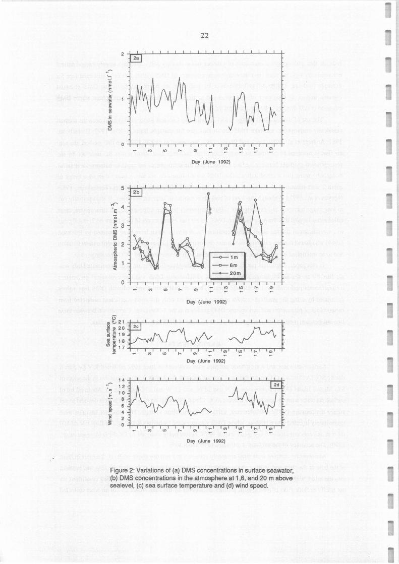
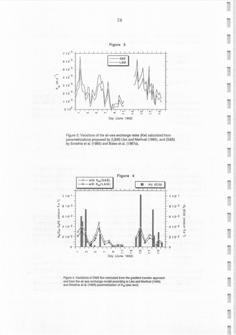
(4) and (5) K.v(L&M) values for DMS ranging from 1.0 10-6 to 5.0 10-sm.s-1 (mean 1.9 10-s, Figure 3).
ii. Smethie and al. parametrization of Kw (Kw(S&B)
Another parametrization of Kw is based on correlation between Radon piston velocity and wind
speed observed by Smethie et al. (1985) in the Atlantic Ocean, and fitted to take into account results of
laboratory experiments which indicated that piston velocity reaches O for wind speed "" 3 m.s-1 (Broecker
et al., 1978; Wannikhof et al., 1985). For DMS, Kw was calculated by Bates et al. (1987a) from Radon
piston velocity, assuming that exchange coefficients vary with the Schmidt number to the power -1/2
(Holmen and Liss, 1984; Ledwell, 1984). Therefore:
for u~3ms-1 Kw = 7.6 10-6 (u-3) (D/n)l/2 (1.14 10-5 / 1.12)-1/2 (7)
where Kw is obtained in m s-1, other units being the same as in equations (4) and (5). From
. equation (7), we obtained Kw(S&B) exchange coefficients in the range O - 6.6 10-s m s-1 (mean 2.7 10-5,
Figure 3), on average higher by 30% greater than Kw(l.&M) values estimated by equations (4) and (5).
The data reported here confirm the situation usually encountered, where variations in DMS
seawater concentrations are relatively small (factor of 5) in respect with those of transfer velocities (a
~
"! E
;i: :.::
;=-ln
N
~ ë5 E E.
26
Figure 3
7 1 o· 5
s 1 o· 5 ~ M
s 1 o· 5
4 1 o· 5
3 1 o· 5
2 1 o· 5
1 1 o· 5
0 1 o0
C') Il) ,._ 0) C') Il) ,._ 0)
Day (June 1992)
Figure 3: Variations of the air-sea exchange rates (Kw) calculated from parametrizations proposed by (L&M) Liss and Merlivat (1986), and (S&B) by Smethie et al. (1985) and Bates et al. (1987a).
Figure 4 ---o-- with Kw(S&B) --with Kw(l&M) • -Kz àCtàz 1
1 1 o· 1 1 1 o· 1
a 1 o· 2 a 10-2
s 1 o· 2 s 1 o- 2
~ 4 10-2 4 1 0-2
4 .J 2 1 0-2
0 C') Il) ,._ a, - C') Il) ,._ a,
Day (June 1992)
Figure 4: Variations of DMS flux estimated from the gradient transfer approach and from the air-sea exchange model according to Liss and Merlivat (1986) and Smethie et al. (1985) parametrization of Kw (see text) .
2 1 o· 2
0
~ N .... (') èi:; N
:, 3 !2. ~ _..., "\ ~
_,..
-
-
27
factor of ""50). According to equation (2), the DMS sea-air flux were Ülerefore controlled by the sea-air
exchange rate rather than by the amount of DMS available at Ûle ocean surface. Using equation (2) with
Kw and DMS concentrations determined for the same time, we obtained estimates of DMS sea-air flux
plotted on Figure 4, ranging from 5.0 10·4 to 3.5 10·2 nmol m ·2 s·l (mean 1.3 nmol m·2 s·I = 1.1 µmol
m·2 day·I) or from 2.0 10-4 to 4.7 10·2 nmol m·2 s·l (mean 1.8 nmol m-2 s·I = 1.6 µmol m·2 clay·l),
according to Liss and Merlivat (1986) and Smethie et al. (1985) parametrization of Kw, respectively.
These values are significantly smaller than the estimates by Erickson et al. (1990) for this area in July
(""4.5µmol m·2 d 1) calculated from a model based on the correlation between DMS flux and incident solar
radiation observed by Bates et al. (1987b). This difference is partially due to the average DMS
concentration in seawater observed during this experiment which was lower than the mean value of 2.3
estimated by Bates (1987a) for summer at 35°N in the Pacifie ocean. Furthermore, comparison between
the tranfer velocity of C02 computed from Liss and Merlivat (1986) parametrization of Kw and fluxes
determined from 14C02 measurements (Erickson, 1989) indicated that equations (4-5) could underestimate
Kw by a factor of 1.8.
DMSfluxfrom the gradient-tranfer approach
In the gradient-tranfer approach, it is assumed that turbulence causes a positive flux of parameter X
(Fx) down the atmospheric gradient of X concentration, at a rate which is proportionnai to Ûle magnitude
of the gradient by similarity with transfer in laminar flow. For a simple vertical diffusion model, Ülis can
be written:
Fx(z) = -Kz(z) aX(z)/az (8) where z is the altitude (in m), and ~ the eddy diffusion coefficient (m2 s·I ).
For DMS, assuming that the contribution of atmospheric oxidation in DMS vertical profile is
negligible with respect to the contribution of eddy diffusion (this assumption will be discussed in the
following paragraphs), we can write:
FoMS (z) = -Kz(z) a[DMS]lê)z (9)
Vertical transport evaluation was based on the assumption made by Thompson and Lenschow
(1984) that Ûle eddy diffusion coefficient "Kz(z) is not affected by chemical reactions and that the
dimensionless gradient for mass transfer is equal to that of temperature". Kz(z) can therfore be described by
the equation (Businger et al., 1971):
~(z) = u* k z [0.74 (1-9z/L)·l/2)-1 for z/L<O (10)
with L = u*3<T>/kg<w'0'>
where u* is surface friction velocity (m s·1), k is Ûle dimensionless von Karman constant (0.35), L
is the Monin-Obukhof length (m), <T> is mean atmospheric temperature (K), g is gravitationnal
· àcceleration (m s·2), and <w'0'> is the kinematic surface virtual temperature flux (Km s·1), which was
always >0 (SST> T air) during periods where negative DMS gradients were observed (Table 1). It should be
noted that another analytic form for Kz has been proposed (Dyer and Bradley, 1982), which would have led
to Kz values smaller by Jess than 15% for the range of z/L values encountered during this experiment
day O=w'0' u (mis) u· (mis) Ri L(m) Kz (m2/s) ac;az (nmol/m)
1.50 8.0 0.0059
2.25 0.02513 9.0 0.34099 -0.0207 -116.36 0.643 -0.0928
2.50 0.00605 7.5 0.27782 -0.0080 -262.77 0.488 -0.1014
3.25 0.00646 5.5 0.20477 -0.0284 -98.10 0.395 -0.1861
3.50 0.00611 6.0 0.22204 -0.0193 -132.44 0.413 0.0400
4.25 0.00960 4.0 0.16003 -0.1351 -31.52 0.386 0.0150
4.50 0.00324 4.5 0.16959 -0.0261 -111.62 0.321 -0.0340
5.25 0.00162 5.5 0.20243 -0.0041 -380.31 0.349 -0.0084
5.50 -0.00184 6.0 0.21891 0.0101 423.87 0.344 0.0580
6.25 0.02050 9.0 0.34036 -0.0165 -142.69 0.628 0.0699
6.50 0.01258 9.0 0.33927 -0.0095 -230.72 0.601 -0.0409
7.25 0.01548 7.0 0.26115 -0.0307 -85.31 0.513 0.0400
7.50 0.00414 4.0 0.15464 -0.0532 -66.42 .0.317 0.0312
8.50 0.00739 6.0 0.22251 -0.0238 -110.10 0.423 0.0666
9.25 0.00449 4.0 0.15498 -0.0588 -61 .19 0.322 -0.0085
9.50 0.00029 3.5 0.13468 0.0031 -627.53 0.228 0.0300
10.50 0.00056 3.0 0.06398 -0.6104 -34.78 0.151 0.0270
11 .25 0.00041 4.5 0.16738 0.0019 -859.73 0.281 0.0010
11.50 -0.00344 4.0 0.1469 0.0578 68.66 0.162 0.0449
14.50 0.00342 9.0 0.33802 -0.0015 -837.61 0.568 -0.0337
15.25 0.00190 8.0 0.29674 -0.0007 -1020.78 0.497 -0.0625
15.50 0.00010 8.5 0.31674 0.0017 -22643.11 0.521 -0.1948
16.50 0.00095 8.0 0.29656 0.0006 -2036.64 0.492 0.1490
17.50 0.00586 10.5 0.4032 -0.0019 -834.62 0.678 -0.3888
18.25 0.00272 5.5 0.20295 -0.0094 -228.72 0.360 -0.2029
18.50 0.01289 7.5 0.27935 -0.0195 -125.28 0.522 -0.0415
19.25 0.01041 6.5 0.24143 -0.0260 -100.23 0.464 -0.0220
19.50 0.00802 6.0 0.22275 -0.0259 -102.33 0.427 -0.0669
20.25 0.00738 6.0 0.22251 -0.0238 -110.60 0.422 -0.0223
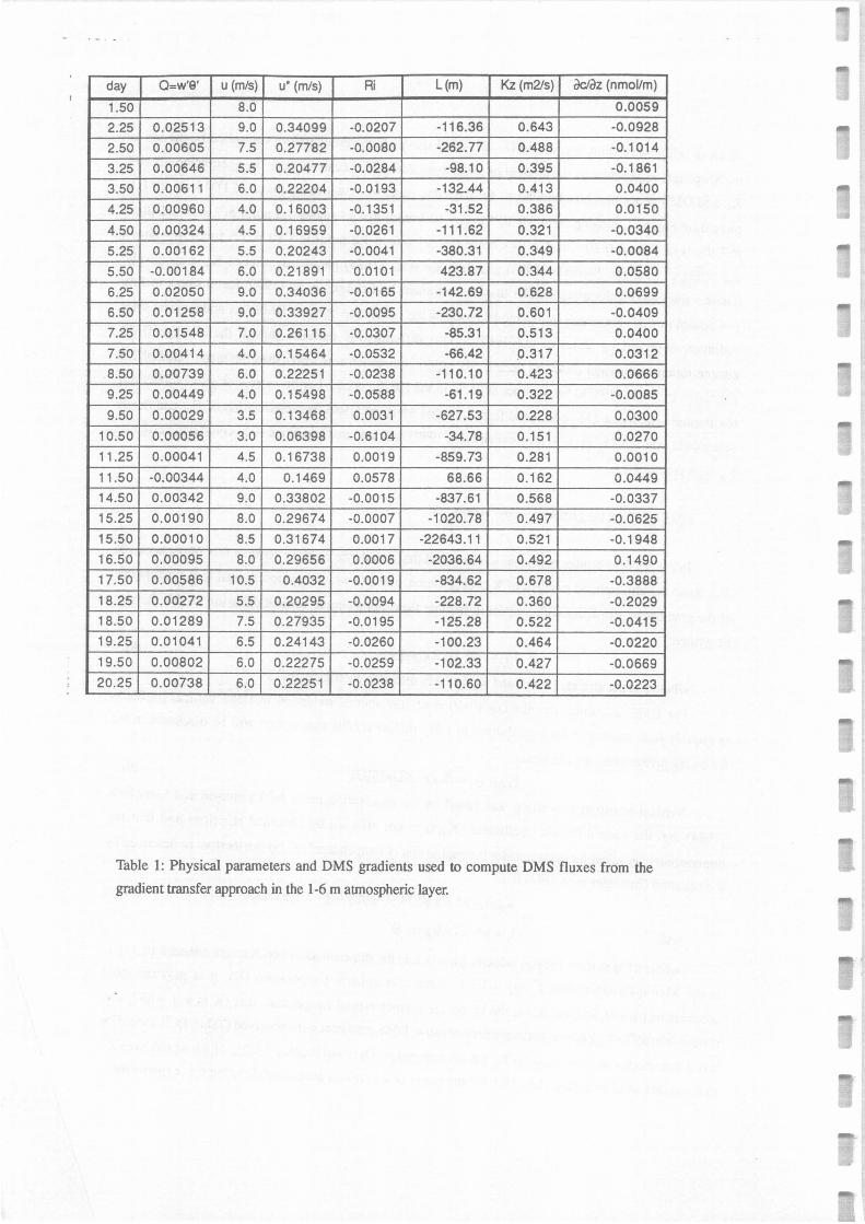
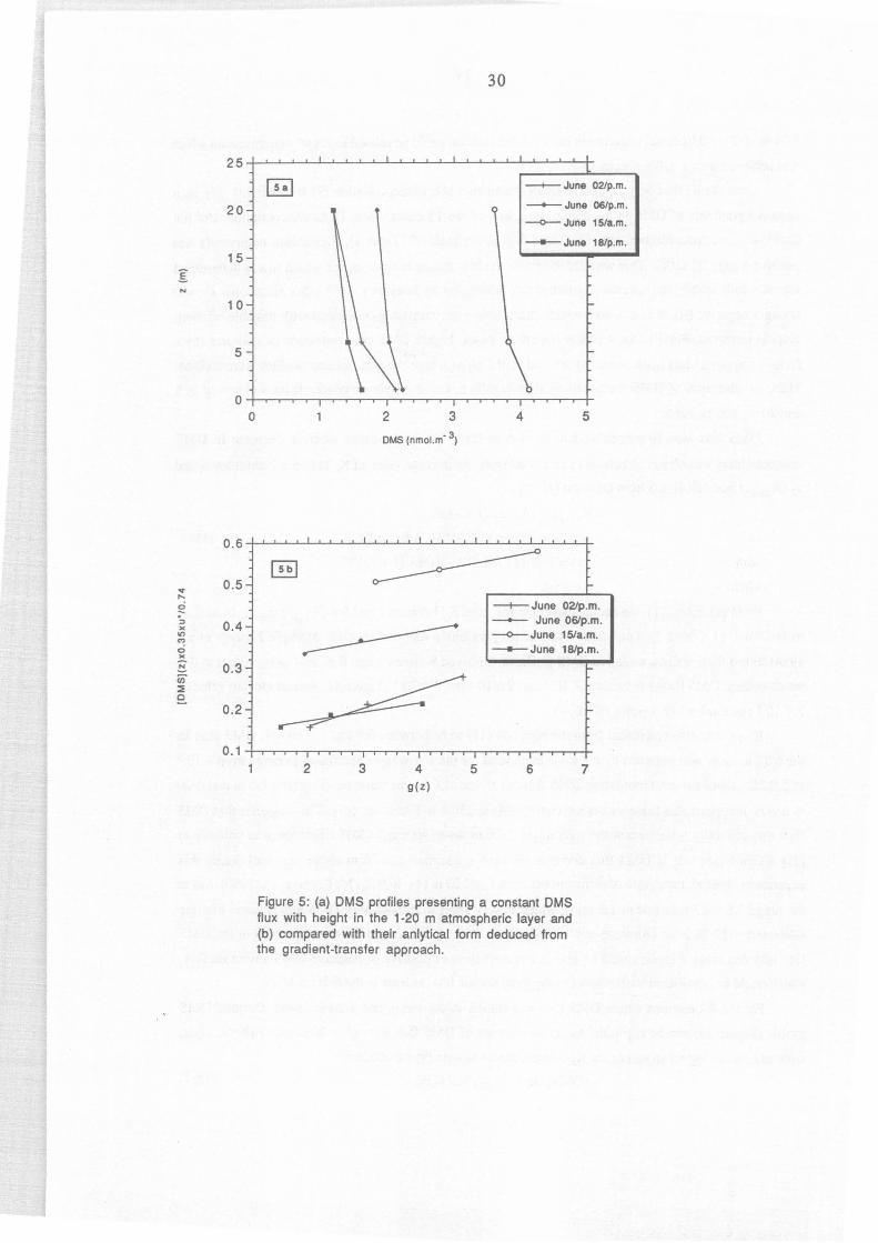
Table 1: Physical parameters and DMS gradients used to compute DMS fluxes from the
gradient transfer approach in the 1-6 m atmospheric layer.
-•
29
0.01 to -0.3). Additionna! uncertainty on K 2 detennination could be related to the u* detennination which
was achieved with a ±10% accuracy.
Considering that only a positive DMS sea-air flux is realistic, equation (9) is consistent only with
negative gradients of DMS in the atmosphere. In 7 of the 13 cases where DMS concentrations did not
decrease in its concentration between 1 and 6 m above sealevel (Table 1 ), Richardson number Ri was
positive (range O - 0.06). This was denoting that the low atmospheric layer for which it was detennined
was statically stable, thus preventing turbulence generation by bouyancy. In 2 other situations, Ri was
strongly negative (-0.14 and -0.65), which characterizes very unstable conditions with possible efficient
vertical transport. Finally, for 4 of the remaining cases, higher DMS concentrations in seawater (by a
factor of about 2) had been observed upwind of the point where the atmospheric profiles were studied.
Thus, an advection of DMS, contributing significantly to the atmospheric concentrations observed at 6
and 20 m, was possible.
DMS flux was first caculated in the 1-6 m layer for the 16 cases where a decrease in DMS
concentrations was observed between these two levels. An average value of~ between 2 altitudes z1 and
'Li (K21 _22) was calculated from equation (10) by:
i.e .
with
where
Kz1 _22 = 1/(zrzi) f Kz(z)dz
K21 _22 = l/(zrz1) 0.35u*/0.74 [f(z2)-f(z1)]
f(z) = 2z/38 (1 + 8z)3/2 -4/1582 (1 + 8z)5/2
8=-9/L
(11)
From equation {11), we obtained average values of K 2 between 1 and 6m (K 1_6) ranging from 0.32
to 0.47 m2 s-1 (Table 1), consistent with values previously reported (see for example Nguyen et al.,
1984). From these values, negative DMS gradients observed between 1 and 6 m, and using equation (9),
we calculated DMS fluxes between 2.7 10-3 and 2.6 10-1 nmol m2 s-1 (Figure 4), with an median value of
2.7 10-2 nmol m2 s-1 (2.3 µmol m2 œy-1).
~-2o was also calculated from the equation {l 1) to be between 0.8 and 3.0 m2 s-1. DMS flux in
the 6-20 m layer was obtained by the same method as for the 1-6 m layer and found to range from 4 10-5
to 2.0 10-1 nmol m2 s-1. Comparing DMS fluxes calculated from the same profile in the 1-6 m and 6-20
m layers, it appears that these values are comparable at ±30% in four cases only. This suggests that DMS
flux was generally not constant throughout the 1-20 m layer, although DMS oxidation was unlikely to
play a significant role in DMS flux decrease between sea surface and 20 m above sea-level during this
experiment. Indeed, time scale of diffusion between 1 and 20 m (t = h2/4~. McKeene et al., 1990) was in
the range 0.6 - 2.3 min (mean 1.1 min), which is very short in respect with DMS atmospheric lifetime
estimated at 12-36 hour (Andreae et al., 1988; Bates et al., 1990). The difference observed in the DMS
flux between these 2 layers could be due to a contribution of positive or negative DMS advection flux,
which could be significant with respect to the local sea-air flux, at least in the 6-20 m layer.
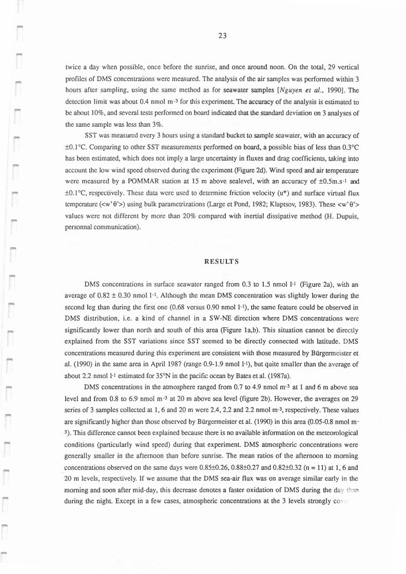
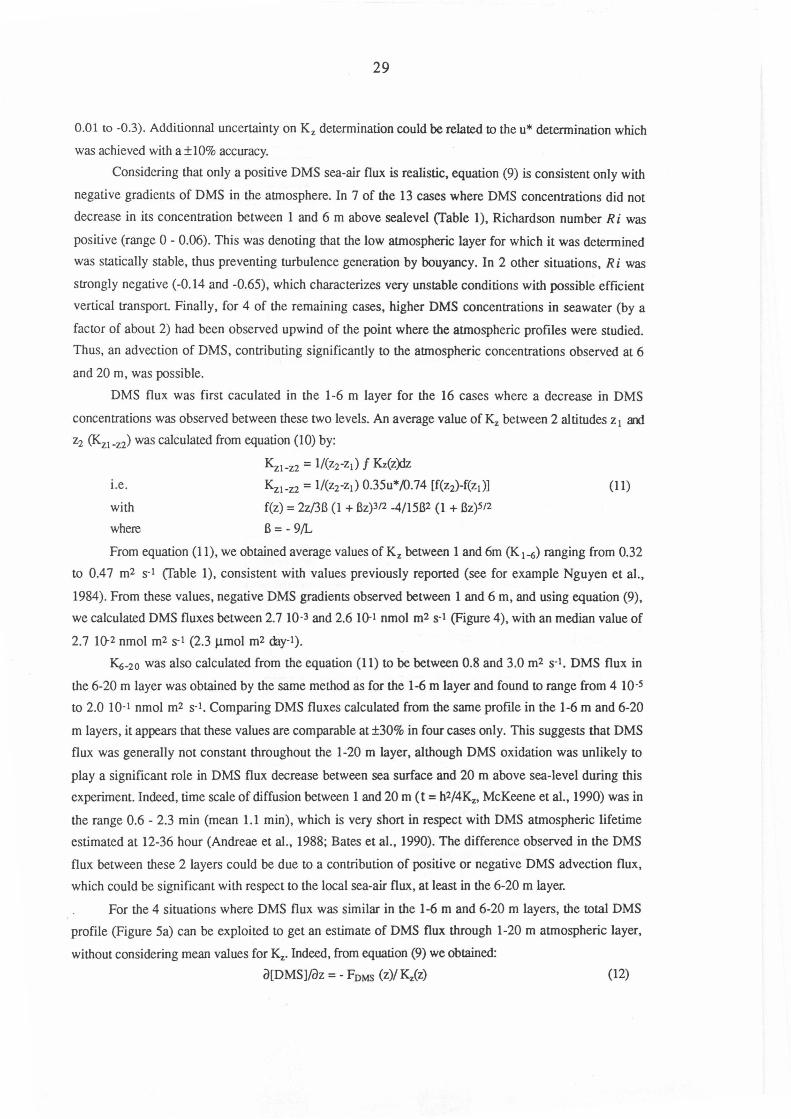
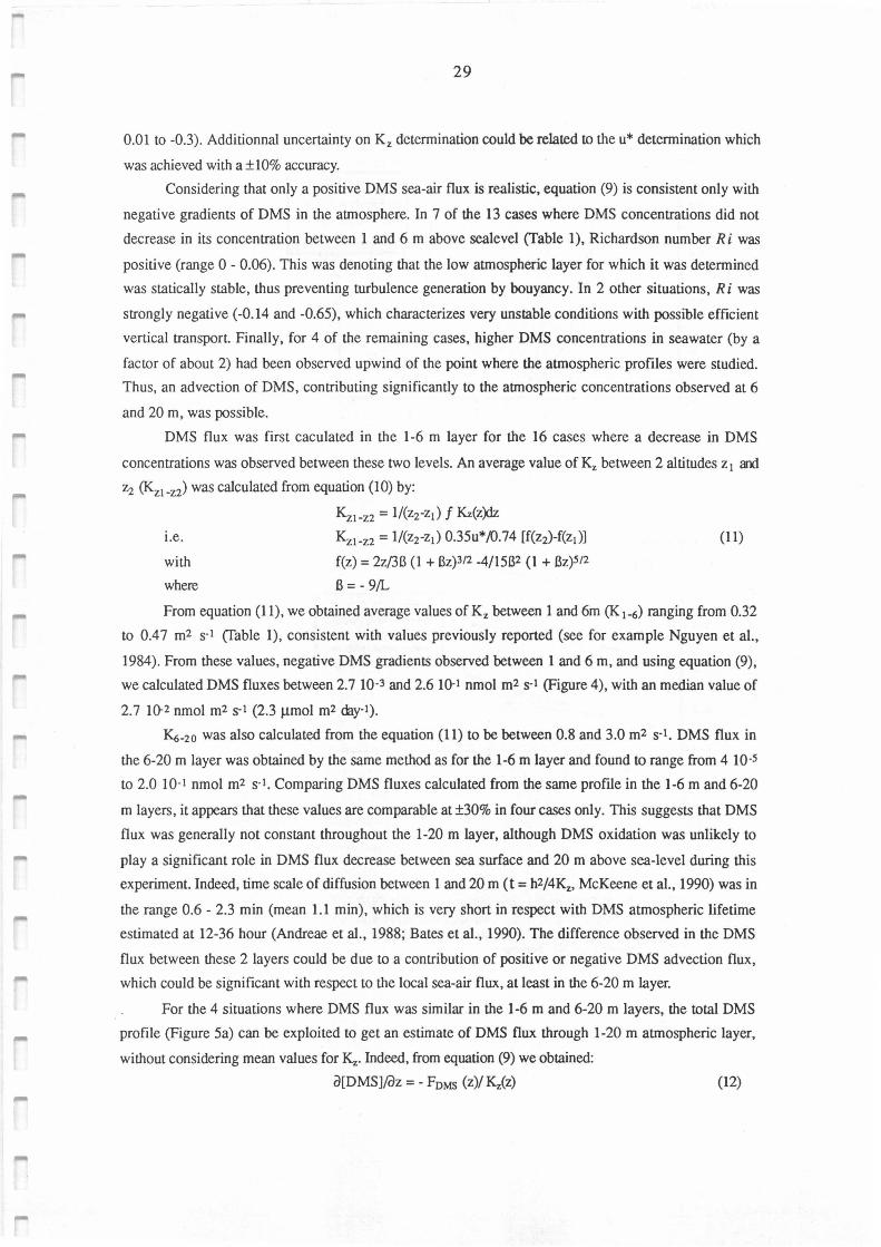
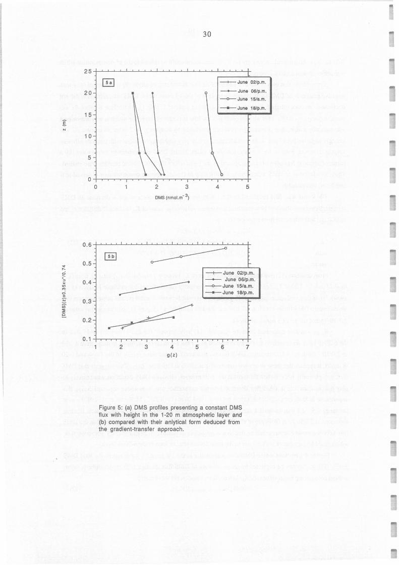
For the 4 situations where DMS flux was similar in the 1-6 m and 6-20 m layers, the total DMS
profile (Figure Sa) can be exploited to get an estimate of DMS flux through 1-20 m atrnospheric layer,
without considering mean values for~- Indeed, from equation (9) we obtained:
a[DMS]/az = - FoMS (z)/ ~(z) (12)
25
20
15
I N
1 0
5
0 0
0.6
.., 0.5 ,._ !2 ':,
0.4 )C
"' .., 0 )C
E 0.3 U) :::E e.
0.2
0.1 1
~
~
2 3
2 3
OMS (nmo1.m· 3)
4 g(z)
5
30
--+-- June 02/p.m.
--June 06/p.m.
-<>-- June 15/a.m.
- June 18/p.m.
4 5
--+- June 02/p.m. -- June 06/p.m. -<>--June 15/a.m. - June 18/p.m.
6 7
Figure 5: (a) OMS profiles presenting a constant OMS flux with height in the 1-20 m atmospheric layer and (b) compared with their anlytical form deduced from the gradient-transfer approach.
29
0.01 to -0.3). Additionnal uncertainty on Kz determination could be related to the u* determination which
was achieved with a ± 10% accuracy.
Considering that only a positive DMS sea-air flux is realistic, equation (9) is consistent only with
negative gradients of DMS in the atmosphere. In 7 of the 13 cases where DMS concentrations did not
decrease in its concentration between 1 and 6 m above sealevel (Table 1), Richardson number Ri was
positive (range 0 - 0.06). This was denoting that the low atmospheric layer for which it was determined
was statically stable, thus preventing turbulence generation by bouyancy. ln 2 other situations, Ri was
strongly negative (-0.14 and -0.65), which characterizes very unstable conditions with possible efficient
vertical transport. Finally, for 4 of the remaining cases, higher DMS concentrations in seawater (by a
factor of about 2) had been observed upwind of the point where the atmospheric profiles were studied.
Thus, an advection of DMS, contributing significantly to the atmospheric concentrations observed at 6
and 20 m, was possible.
DMS flux was first caculated in the 1-6 m layer for the 16 cases where a decrease in DMS
concentrations was observed between these two levels. An average value of Kz between 2 altitudes z 1 and
'Li (Kz1-z2) was calculated from equation (10) by:
i.e.
with
where
Kz1-z2 = l/(zrz1) f Kz(zx)z
Kz1 -z2 = l/(zrz1) 0.35u* /0. 74 [f(z2)-f(z1 )]
f(z) = 2z/3B (1 + Bz)3/2 -4/1582 (1 + Bz)5/2
B = - 9/1...
(11)
From equation (11), we obtained average values of Kz between 1 and 6m (K 1-6) ranging from 0.32
to 0.47 m2 s-1 (fable 1), consistent with values previously reported (see for example Nguyen et al.,
1984). From these values, negative DMS gradients observed between 1 and 6 m, and using equation (9),
we calculated DMS fluxes between 2.7 10-3 and 2.6 10-1 nmol m2 s-t (Figure 4), with an median value of
2.7 10-2 nmol m2 s-t (2.3 µmol m2 œy-t).
~-2o was also calculated from the equation (11) to be between 0.8 and 3.0 m2 s-t. DMS flux in
the 6-20 m layer was obtained by the same method as for the 1-6 m layer and found to range from 4 10-5
to 2.0 10-1 nmol m2 s-t. Comparing DMS fluxes calculated from the same profùe in the 1-6 m and 6-20
m layers, it appears that these values are comparable at ±30% in four cases only. This suggests that DMS
flux was generally not constant throughout the 1-20 m layer, although DMS oxidation was unlikely to
play a significant role in DMS flux decrease between sea surface and 20 m above sea-level during this
experiment. Indeed, time scale of diffusion between 1 and 20 m (t = h2/4~, McKeene et al., 1990) was in
the range 0.6 - 2.3 min (mean 1.1 min), which is very short in respect with DMS atmospheric lifetime
estimated at 12-36 hour (Andreae et al., 1988; Bates et al., 1990). The difference observed in the DMS
flux between these 2 layers could be due to a contribution of positive or negative DMS advection flux,
which could be significant with respect to the local sea-air flux, at least in the 6-20 m layer.
For the 4 situations where DMS flux was similar in the 1-6 m and 6-20 m layers, the total DMS
profile (Figure Sa) can be exploited to get an estimate of DMS flux through 1-20 m atmospheric layer,
without considering mean values for~- Indeed, from equation (9) we obtained:
a[DMS]/az = - FoMS (z)/ ~(z) (12)
25
20
1 5 :[ N
10
5
0 0
0.6
... 0.5 ,-..
~ •:,
0.4 )(
"' ~ 0 )(
N 0.3 en :!? e.
0.2
0. 1 1
~
@]
2 3
2 3
OMS (nmo1. m· 3)
4 g(z)
5
30
- June 02/p.m.
-+-- June 06/p.m.
-o--June 15/a.m.
-+-June 18/p.m.
4 5
--+- June 02/p.m. -+-- June 06/p.m. -o-- June 15/a.m. -+-June 18/p.m.
6 7
Figure 5: (a) OMS profiles presenting a constant OMS flux with height in the 1-20 m atmospheric layer and (b) compared with their anlytical form deduced from the gradient-transfer approach.
,...
31
As FnMs can be considered as constant between 1 and 20 m height, an analytical fonn of [DMS](z)
can be established by integrating (12):
[DMS](z) = -0.74 FoMS / 0.35 u* g(z) + A
where g(z) = ln [(1 + Bz)t /2...±.li, and Ais a constant coming from the integration.
(1 + Bz)t/2 -1)
(13)
Therefore FnMs could be estimated from the slope of the plots representing -0.35 u*[DMS](z)/0.74
versus g(z) presented on Figure Sb. It appears that equation (13) can adequately reproduce these 4 profiles
since the coefficient of linear regressions are ail R2~0.99. The values of DMS flux calculated by this
method are similar (±20%) to the values calculated for the same time from equation (9) in the 1-6 m
layer, which indicates that averaging K 2 in this layer can lead to reliable estimates of DMS flux. Taking
into account the accuracy of u* determination (±10%), the uncertainty introduced in using K2 values
averaged between 1 and 6 m height (±20%), and the uncertainty on DMS gradient determination (±15%),
DMS fluxes obtained by the gradient method present a global uncertainty of± 45%.
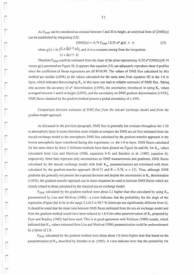
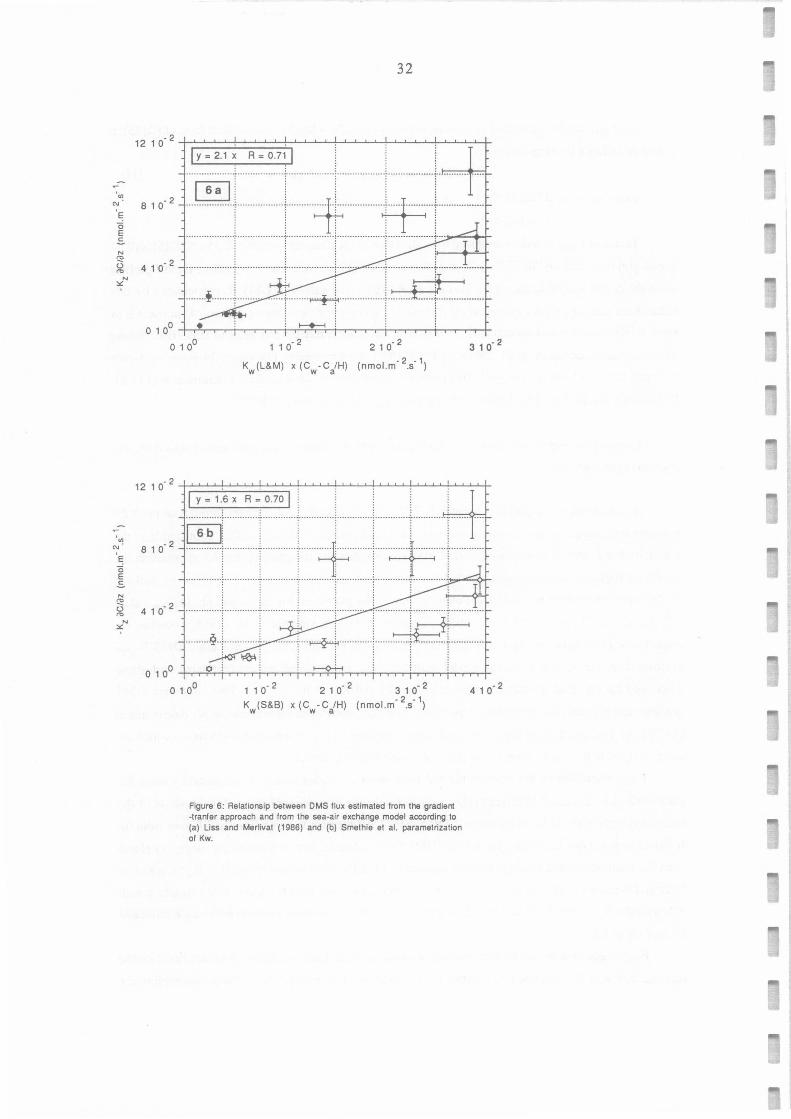
Comparison between estimates of DMS flux /rom the sea-air exchange mode! and /rom the
gradient-tranfer approach.
As discussed in the previous paragraph, DMS flux is generally not constant throughout the 1-20
m atmospheric layer. IL seems therefore more reliable to compare the DMS sea-air flux estimated from the
sea-air exchange mode! Lo the atmospheric DMS flux calculated by the gradient-transfer approach in the
lowest atmospheric layer considered during this experiment, i.e. the 1-6 m layer. DMS fluxes calculated
for the same times by these 2 different methods have been plotted on Figure 6a and 6b, for Kw values
calculated from Liss and Merlivat (1986, equations 4-5) and Smethie et al. (1985, equation 6),
respectively. Error bars represent only uncertainties on DMS measurements and gradients. DMS fluxes
calculated by the sea-air exchange model with both Kw parametrizations are correlated with those
calculated by the gradient-transfer approach (R=0.71 and R = 0.70, n = 15). Thus, although DMS
gradients did generally not present the expected decrease and despite the uncertainties in K2 detennination
(±45%), the gradient-transfer approach can in some situations be used to estimate DMS fluxes which are
closely related to those calculated by the classical sea-air exchange mode!.
FoMs calculated by the gradient method were about 2.1 higher than that calculated by using Kw
parametrized by Liss and Merlivat (1986) : a t-test indicates that the probability for the slope of the
regression (Figure 6a) to be in the range 2.1±0.5 is 99.7 % (intercept not significantly different from 0).
It should be noted that the mean ratio between DMS fluxes estimated from the sea-air exchange mode! and
from the gradient method would have been reduced to 1.8 if the other parametrization of K 2 proposed by
Dyer and Bradley (1982) had been used. This is in good agreement with Erickson (1989) results, which
indicated that K w values estimated from Liss and Merlivat (1986) parametrization could be underestimated
by a factor of 1.8.
FoMs calculated by the gradient method were about about 1.6 times higher than that based on the
parametrization of Kw described by Smethie et al. (1985). At-test indicates here that the probability for
' en N .
'E
0 E .s N
(1: (.)
"" N ~
32
: : : : : ---4
~ ! ! ! ! : ···················1··················i-········~·············rt= ··1··················
. . . . ' ' ' ' . ' ' ' . . ' ' ' . ~ l l : : . : : ··· ···':. ·················· :··················
.... + ........ ! ......... ~ ·······~ ··················:·' ....... i ...... 1~ ............... . 0 1 o0 -+--r'-r-r--r--+--r--,c--r--r--t!--r-,-r'•'r-1r--t-:--r-~T""-.-+: --r--,-r-r-t-~-r--,.-,.--+-
o 1 o0
12 10· 2 ~:::::::::::=:::=::=:::::'.::~~.._.__-'--t~~"t--'-........... --'--t...,__....,__.T~~ Y=1 .6x R=0.70I
: : : : : ! ~.--C>-1
~ ; ; : ; ; ;
1 i 1+ iT~i ~ ! : ! ·· ············-· ············- ··········· ··
: : : :~ : : : ~ ,
········;···~ ·············;·············:············;·············
0 1 0 0 -+-r-r--r.-r-r-r-.-r-r-,c-rr,-r. -,-,l--0-H,-r,.:-r-,r,r,i ,.-,-.-,-,-i .-r.,.-,r-r-i .-r-r-i-+-0 1 o0
11~2
21~2
31~2
Kw(S&B) x(C - C/H) (nmol.m·2.s·
1)
w a
Figure 6: Relationsip belween OMS flux estimated from the gradient -tranfer approach and from the sea-air exchange modal according to (a) Liss and Merlivat (1986) and (b) Smethie et al. parametrization of Kw.
4 1 o· 2
-
33
the slope of the regression (Figure 6b) to be out of the range 1.6±0.4 is only 0.4 % and that the intercept
is once more not significantly different from O. The other parametrization of K2 proposed by Dyer and
Bradley (1982) would have led to a slope of only 1.3. Therefore, using an sea-air exchange mode! with the
parametrization of Kw described by equation (7) very probably leads to an underestimate of DMS sea-air
flux by up to a factor of 2. The most recent estimate for global DMS sea-air flux (Bates et al., 1992) is
0.48±0.33 Tmol/a (15±10TgS/a), with only ±30% of the uncertainty coming from regional average
estimates of DMS concentrations in seawater. If the correlation (Figure 6b) resulting from data obtained
with wind speed in the range 3-10 m s-1 could be extrapolated to higher wind speeds, mainly observed in
the southern hemisphere, the global DMS sea-air flux could be reevaluated to 0.64 -0.76 Tmol/a (20-24
TgS/a), with an uncertainty of ±0.15-0.17 Tmol/a (a: 5TgS/a).
The validity of these results is of course dependent on the reliability of the gradient-tranfer
approach to determine DMS fluxes. Although the significant correlations observed (Figure 6a,b) could be
considered as an evidence of this assumption, large uncertainties (±45%) are introduced in DMS flux
calculation from the gradient method. It should be noted that the difference between DMS fluxes estimated
by the gradient and the sea-air exchange methods could be due not to the analytical forms giving KW' but
to the value of DMS diffusivity in seawater predicted from tables, which has never been directly
measured. More accuracy in DMS flux calculation should be achieved in using the eddy correlation
method during specifically planned experiments allowing performance of high frequency atmospheric
DMS measurements.
CONCLUSION
DMS atmospheric profiles observed in the 1-20m layer over the Atlantic Ocean in June 1992
cannot be generally interpreted as resulting from a simple vertical eddy diffusion, although
photochemistry was unlikely to significantly affect DMS gradients. In numerous cases, some
explaination can be suggested such as stable conditions preventing turbulence generation by bouyancy, or
possible fast vertical transport. Advection of air masses from neighbouring areas where DMS emission
was significantly different could also contribute to the observed atmospheric DMS concentrations,
particularly at 20m height. Therefore, the gradient-transfer approach can be used to determine DMS flux
in some specific meteorological situations only. Indeed, only four among the 29 profiles performed in the
1-20 m atrnospheric layer could be fitted by an analytical form deduced from the gradient-tranfer approach
and assuming a constant DMS flux in this layer. These fluxes compare well (±20%) with the estimates of
DMS flux in the 1-6 m layer calculated using averaged values of eddy diffusion coefficient between these
2 levels. The 15 values of DMS flux calculated by the gradient-transfer approach in cases where a decrease
in DMS was observed in the 1-6 m layer were compared with DMS sea-air flux values obtained from the
sea-air exchange mode! for the same instant. These DMS fluxes estimated by 2 completely independent
methods show a significant correlation (R = 0.7, n=15), with intercept not significantly different from O.
The slopes of the regressions indicate that the gradient-transfer approach lead to estimates of DMS flux
higher by a factor of 1.8-2.1 and 1.3-1.6 than the use of the parametrization of the sea-air exchange
34
coefficient by Liss and Merlivat (1986) and Smethie et al. (1985), respectively. This confirms the
suggestion of Erickson et al. (1990) that Kw values estimated from Liss and Merlivat (1986)
parametrization could be underestimated by a factor of 1.8. Taking into account that the most recent
estimate of global DMS oceanic flux (0.48±0.33 TmoVa , i.e. 15±10 TgS/a) reported by Bates et al.
(1992) was based on Smethie et al. (1985) parametrization of Kw, this figure could be reevaluated by a
factor of up to 2. However, large uncertainties introduced in the DMS flux calculation by the gradient
approach method (±45%) prevent these results being considered as definitive.
Acknoledgments. We thank the officers and the crew of the IFREMER ship Le Suroît for their
cooperation. This work was supported by the Centre National de la Recherche Scientifique, the Commissariat à
l 'Energie Atomique and the Ministère de la Recherche et de la Technologie. This is CFR contribution xxxx.
REFERENCES
Andreae, M.O., The ocean as a source of atmospheric sulfur compounds, in The Role of sea-air
Exchange in Geochemical Cycling, edited by P. Buat-Ménard, pp. 331-362, D. Reidel, Horwell,
Mass., 1986.
Andreae, M.O., Beresheim, H., Andreae, T.W., Kritz, M.A., Bates, T.S., and Merill, J.T., Vertical
distribution of dimethylsulfide, sulfur dioxide, formic acid, aerosol ions, and radon over the northeast
Pacifie ocean,J. Atmos. Chem., 6, 149-173, 1988.
Aneja, V.P. and Overton, J.H., The emission rate of dimethylsulfide at the atmospheric-oceanic interface,
Chem. Eng. Comm, 98, 199-209, 1990.
Bates, T.M., J.D. Cline, R.H. Gammon and S.R. Kelly-Hansen, Regional and seasonal variation of the
flux of oceanic dimethylsulfide to the atmosphere, J. Geophys. Res., 92, 2930-2938, 1987a.
Bates, T.S., R.J. Charlson and R.H. Gammon, Evidence for the climatic role of marine biogenic sulphur,
Nature, 329, 319-321,1987b.
Bates, T.S., Johnson, J.E., Quinn, P.K., Goldan, P.D., Kuster, W.C., Covert, D.C., and Hahn, C.J., The
biogeochemical cycle in the marine boundary layer over the northeast Pacifie ocean, J. Atmos.
Chem., 10, 59-81, 1990.
Bates, T.S., B.K. Lamb, A.B. Guenther, J. Oignon, E.S. Stoiber, Sulfur emissions to the atmosphere
from natural sources, J. Atmos. Chem., 14, 315-337, 1992.
Belviso, S., Kim, S.K., Rassoulzadegan, F., Krajka, B., Nguyen, B.C., Mihalopoulos, N., and Buat-
Menard, P. Production of dimethylsulfonium propionate (DMSP) and dimethylsulfide (DMS) by the
microbial food web, Limnol. Oceanogr., 35, 1810-1821, 1991.
Berresheim, H., Biogenic sulfur emissions from the subantarctic and antarctic oceans, J. Geophys. Res.,
92, 13245-13262, 1987.
Broecker, H.C.,and Siems, W., The role of bubbles for gas transfer from water to air at higher wind
speeds. Experiments i the wind-wave facility in Hamburg., in Brutsaert and Jirka (Eds), Gas tranfert at
water surfaces, D. Reidel, Dordrecht, 229-236, 1984.
Bürgermeister, S. , R.L. Zimmerman, H.W. Georgii, H.G. Bingemer, G.O. Kirst, M. Jansen, W. Ernst,
,....
35
On the biogenic origin of dimethylsulfide: relation between chlorophyll, ATP, organismic DMSP,
phytoplancton species, and DMS distribution in Atlantic surface seawater and atmosphere, J.
Geophys. Res., 95, 20607-20615, 1990.
Businger, J.A., Wyngaard, J.C., Izumi, T and Bradley, E.F., Flux-profile relationships in the atrnospheric
surface layer,]. Atmos. Sei. , 28, 181-189, 1971.
Charlson R.J., J.E. Lovelock, M.O. Andreae, S.G. Warren, Oceanic phytoplankton, atrnospheric sulphur,
cloud albedo and climate, Nature, 326, 655-661 , 1987.
Dacey, J.W.H., Wakeham, S.G., and Howes, B.L., Henry's law constant for dimethylsulfide in freshwater
ans seawater, Geophys. Res. Lett .. 11 , 991-994, 1984.
Dacey, J .W .H. and Wakeham, S.G., Oceanic dimethylsulfide: production during zooplankton grazing on
phytoplankton, Science, 233, 1314-1316, 1986.
Dyer, A.J. and Bradley, E.F., An alternative analysis of flux-gradient relationships at the 1976 ITCE,
Boundary-layer Meteorol., 22, 3-19, 1984.
Erickson, D.J., III, Variations in the global sea-air transfer velocity field of CO2, Global. Biogeochem.
Cycles, 3, 37-41, 1989.
Erickson, D.J ., III , Ghan, S.J., and Penner, J.E., Global ocean-to-atmosphere dimethyl sulfide flux, J.
Geophys. Res. , 95, 7546-7552, 1990.
Hayduck, W., and Laudie, H., Prediction of diffusion coefficients for nonelectrolytes dilute aqueous
solutions, Am. Inst. Chem. Eng. J., 20, 611-615, 1974.
Holmen, K., and Liss, P. , Models for air-water gas tranfer: An experimental investigation, Tel/us, 36B,
92-100, 1984.
Keller, M.D., W .K. Bellows, R.R.L. Guillard, Dimethylsulfide production in marine phytoplancton, in
Biogenic Sulfur in the Environment, pp. 167-182, edited by Saltzman E.S. and Cooper W.J.,
American Chemical Society Symposium Series N° 393, Washigton DC, 1989 .
Klaptsov, 1983.
Langner, J. and H. Rhode, A global three-dimensionnal mode! of the tropospheric sulfur cycle, J.
Atmos. Chem., 13, 225-263, 1991.
Large and Pond, 1982.
Leck, C. and Rhode, H., Emiss ions of marine biogenic sulfur to the atrnosphere of northem Europe, J.
Atmos. Chem., 12, 63-87, 1991.
Ledwell, J.R., The variation of the gas transfer coefficinet with molecular diffusivity, in Brutsaert and
Jirka (Eds), Gas tranfert at water surfaces, D. Reidel, Dordrecht, 293-302, 1984.
Liss, P.S. and Slater, P.G., Flux of gases across the sea-air interface, Nature, 247, 181-184, 1974.
Liss, P.S . and Merlivat, L., sea-air gas exchange rates: Introduction and synthesis, in The Raie of se a-air
Exchange in Geochemical Cycling, edited by P. Buat-Ménard, pp. 113-128, D. Reidel, Horwell,
Mass., 1986.
McKeen, S.A., Trainer, M., Hsie, E.Y., Tallamraju, R.K., and Liu, S.C., On the indirect determination
of atmospheric OH radical concentrations from reactive hydrocarbon measurements, J. Geophys. Res ..
95, 7493-7500, 1990.
36
Monfray, P., Echanges océan-atmosphère du gaz carbonique: variabilité avec l'état de la mer, Ph. D.
Thesis, Université de Picardie, 1987.
Nguyen, B.C., Bergeret, C. and Lambert, G., Exchange rates of dimethylsulfide between ocean and
atmosphere, in Brutsaert and Jirka (Eds), Gas tranfert at water surfaces, D. Reidel, Dordrecht, 539-545,
1984.
Nguyen, B.C., S. Belviso, N. Mihalopoulos, J. Gostan and P. Nival, Dimethylsulfide production during
natural phytoplanktonic blooms, Marine Chem., 24, 133-141, 1988.
Nguyen, B.C., N. Mihalopoulos, and S. Belviso, Seasonal variation of atmospheric dimethyl sulfide at
Amsterdam Island in the southem lndian Ocean,J. Aunos. Chem., 11, 123-143, 1990.
Nguyen, B.C., Mihalopoulos, N., Putaud, J.P., Gaudry, A., Gallet, L., Keene, W.C., Galloway, J.N.
Covariation in oceanic dimethylsulfide, its oxidation products and rain acidity at Amsterdam Island in
the southem lndian Ocean. J. Atmos. Chem., 15, 39-53, 1992.
Smethie, W.M.Jr, Takahashi, T., Chipman, D.W., and Ledwell, J.R., Gas exchange and co2 flux in the
tropical Atlantic Ocean determined from 222Rn and pCO2 measurements, J. Geophys. Res., 90, 7005-
7022, 1985.
Thompson, A.M., and Lenschow D.H., Mean profiles of trace reactive species in the unpolluted marine
surface layer, J. Geophys. Res., 89, 4788-4796, 1984.
Wanninkhof, R., Ledwell, J.R., and Broecker, W.S., Gas exchange-wind speed relation measured with
sulfur hexafluoride on a lake, Science, 227, 1224-1226, 1985.
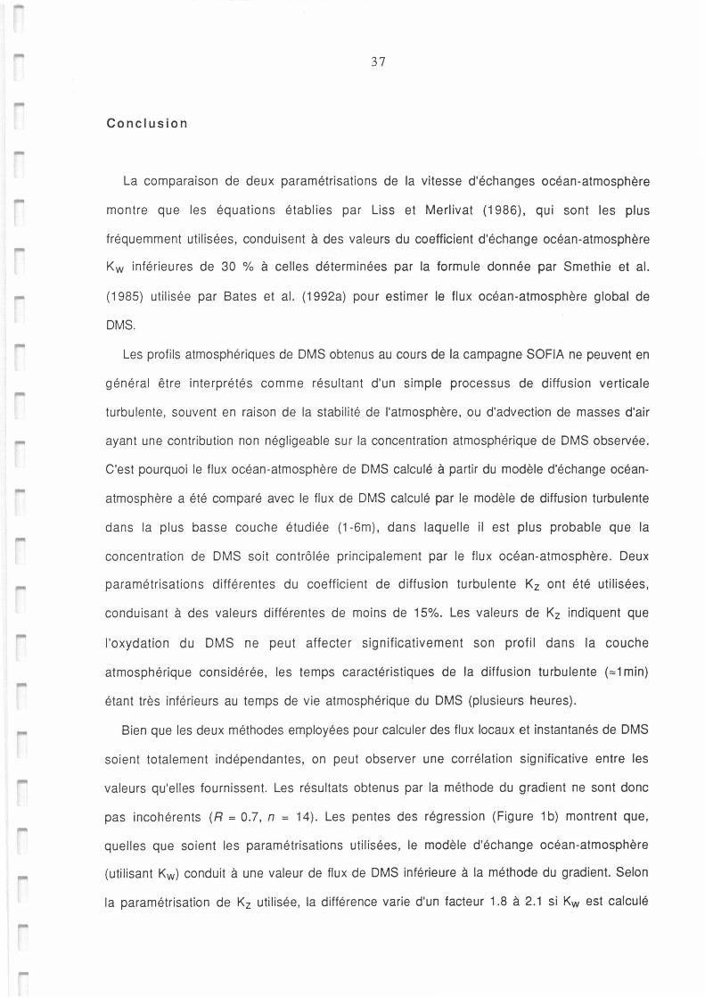
37
Conclusion
La comparaison de deux paramétrisations de la vitesse d'échanges océan-atmosphère
montre que les équations établies par Liss et Merlivat (1986), qui sont les plus
fréquemment utilisées, conduisent à des valeurs du coefficient d'échange océan-atmosphère
Kw inférieures de 30 % à celles déterminées par la formule donnée par Smethie et al.
(1985) utilisée par Bates et al. (1992a) pour estimer le flux océan-atmosphère global de
OMS.
Les profils atmosphériques de OMS obtenus au cours de la campagne SOFIA ne peuvent en
général être interprétés comme résultant d'un simple processus de diffusion verticale
turbulente, souvent en raison de la stabilité de l'atmosphère, ou d'advection de masses d'air
ayant une contribution non négligeable sur la concentration atmosphérique de OMS observée.
C'est pourquoi le flux océan-atmosphère de OMS calculé à partir du modèle d'échange océan-
atmosphère a été comparé avec le flux de OMS calculé par le modèle de diffusion turbulente
dans la plus basse couche étudiée (1-6m), dans laquelle il est plus probable que la
concentration de OMS soit contrôlée principalement par le flux océan-atmosphère. Deux
paramétrisations différentes du coefficient de diffusion turbulente K2 ont été utilisées ,
conduisant à des valeurs différentes de moins de 15%. Les valeurs de K2 indiquent que
l'oxydation du OMS ne peut affecter significativement son profil dans la couche
atmosphérique considérée, les temps caractéristiques de la diffusion turbulente (==1 min)
étant très inférieurs au temps de vie atmosphérique du OMS (plusieurs heures).
Bien que les deux méthodes employées pour calculer des flux locaux et instantanés de OMS
soient totalement indépendantes, on peut observer une corrélation significative entre les
valeurs qu'elles fournissent. Les résultats obtenus par la méthode du gradient ne sont donc
pas incohérents (R = 0.7, n = 14). Les pentes des régression (Figure 1 b) montrent que,
quelles que soient les paramétrisations utilisées, le modèle d'échange océan-atmosphère
(utilisant Kw) conduit à une valeur de flux de OMS inférieure à la méthode du gradient. Selon
la paramétrisation de K2 utilisée, la différence varie d'un facteur 1 .8 à 2.1 si Kw est calculé
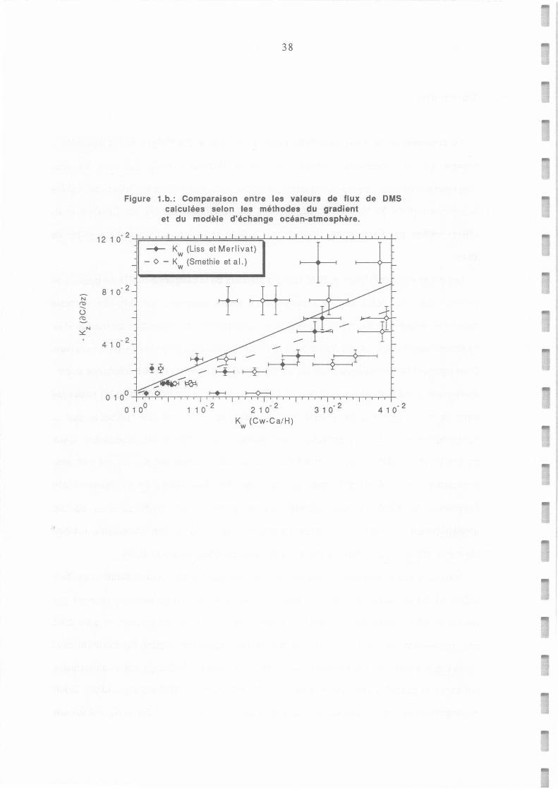
N f't)
ü f't)
N ::s:::
.1
38
Figure 1.b.: Comparaison entre les valeurs de flux de DMS calculées selon les méthodes du gradient
a 1 o· 2
4 1 o· 2
et du modèle d'échange océan-atmosphère.
-+- K (Liss et Merlivat) w
- <> - K (Smethie et al.) w
+* ~---i ~ Il ~ ,2 1
0 1 o0 -+-r-'--T-..,.......~~~~-
1 ~·~
1 ~~t--<>---, ........... ~~~~~~~~~~~~1-
0 1 o0 1 1 o· 2 2 1 o· 2
K (Cw-Ca/H) w
39
par les équations de Liss et Merlivat (1986), et d'un facteur variant de 1.3 à 1.6 en
utilisant la formulation de Kw de Smethie et al. (1985). Bien que la différence de flux
obtenue puisse être due à la formu lation même des équations donnant Kw, au moins en ce qui
concerne la paramétrisation de Liss et Merlivat (1986) (cf Erickson, 1989), il est aussi
probable qu'une valeur érronée de la diffusivité du OMS, qui n'a jamais été directement
mesurée , contribue à l'écart observé . En tout cas, Erickson et al. (1990) ont utilisé des
valeurs de Kw calculées par Liss et Merlivat (1986) augmentées d 'un facteur 1.8 pour
établir une carte mondiale du flux océan-atmosphère de OMS.
Ces résultats pourraient condu ire à réévaluer d'un facteur proche de 2 les valeurs de flux
de OMS rapportées dans la suite de ce travail , calculées à partir des formulations de Kw
proposées par Liss et Merlivat (1986) . De même , l'estimation du flux global de OMS
(15±1 O TgS/an) par Bates et al. (1992a), utilisant la paramétrisation de Kw de Smethie et
al. (1985), pourrait être réévaluée de près de 50%. Cependant, le calcul du flux de OMS par
la méthode du gradient conduit lui aussi à des incertitudes importantes (± 45%) , et un test
statistique sur les corrélations en tre les résultats obtenus par le modèle d'échange océan-
atmosphère et le modèle de diffusion turbulente donne un intervalle de confiance de ± 0.4 à
±0.5 sur la pente des régressions , donc sur le rapport moyen entre les estimations de flux
obtenues par ces deux méthodes. C'est · pourquoi ces résultats demandent à être confirmés,
soit par d'autres campagnes de mesures , soit par une méthode plus directe, comme celle des
"corrélations turbulentes" .

41
LES PRODUITS D'OXYDATION ATMOSPHERIQUE DU SULFURE DE DIMETHYLE.

43
LES PRODUITS D'OXYDATION ATMOSPHERIQUE DU SULFURE DE DIMETHYLE.
Le DMS émis à la surface de l'océan est rapidement oxydé dans l'atmosphère. Des études en
chambres de simulation atmosphérique ont permis d'identifier ses produits d'oxydation
(SO2, MSA, DMSQO), H2SO4, DMSO2(2l) et de proposer des mécanismes réactionnels
détaillés (Figure 2.a). Si le dioxyde de soufre et le diméthylsulfoxyde (SO2 et DMSO) sont
des composés gazeux, les acides méthane sulfonique et sulfurique (MSA et H2SO4) ainsi que
la diméthylsulfone (DMSO2) , de faibles pressions de vapeur saturante , se retouvent
majoritairement dans la phase particulaire. Les proportions de produits formés en chambres
de simulation atmosphérique (Tableau 2.a.) vont de 23 à 70% pour le SO2, de 2 à plus de 50
% pour le MSA et jusqu'à 30% pour le DMSO2 (Hatakeyama et al., 1985; Becker et al.,
1991; Yin et al., 1986, 1990).
Cependant, le devenir des molécules de DMS émises dans l'atmosphère naturelle n'est
encore pas parfaitement connu : alors que les quantités de DMSO et de DMSO2 produites
semblent assez faibles (< 10%; Watts et al., 1987a), les proportions de SO2, MSA, et H2SO4
formées sont variables, dépendant de la concentration de différentes espèces oxydantes (HOx,
NOx, NO3, 03) et de certains paramètres physiques tels que la température de l'air. Nous
avons en effet mis en évidence une augmentation de la proportion de DMS oxydée en MSA
lorsque la concentration en NOx s'élève (Mihalopoulos et al., 1992). Concernant l'influence
de la température, des observations peuvent paraître contradictoires: les mesures effectuées
à différentes latitudes semblent indiquer que la production de MSA est favorisée par les
basses températures. De même, l'analyse des carottes de glace prélevées en Antarctique
montre une augmentation de la proportion MSNnss-SO4 pendant les périodes glaciaires . En
revanche, les cycles saisonniers observés à Cape Grim (Ayers et al., 1991) et à l'île
Amsterdam (Nguyen et al., 1992; ce travail) montrent une augmentation du rapport
MSA/nss-SO4 en été. Mais il n'est pas certain que la chimie atmosphérique soit seule
responsable de ces différences de distribution des produits d'oxydation du DMS. Car si le DMS
semble être l'unique précurseur du MSA, l'acide sulfurique (H2SO4) peut provenir de
1 DMSO = CH3SOCH3
2 DMS02 = CH3S02CH3
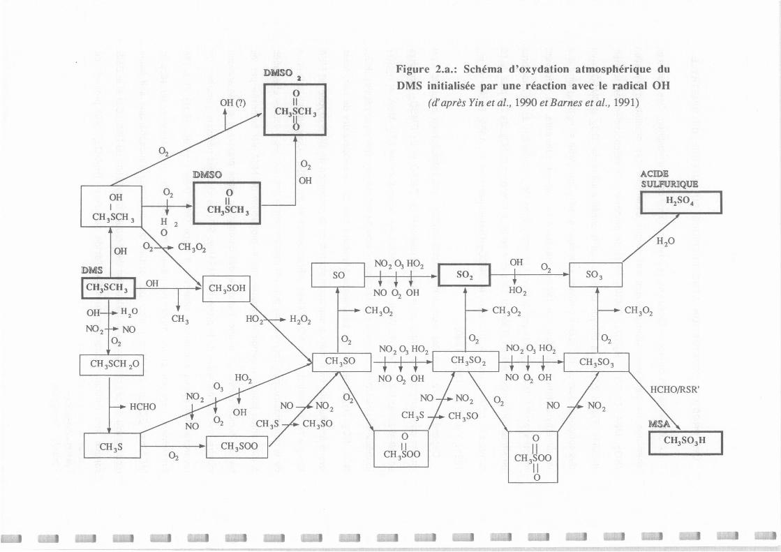
OH(?)
DMISO 2
0 Il
CH3SCH 3
Figure 2.a.: Schéma d'oxydation atmosphérique du
DMS initialisée par une réaction avec le radical OH
(d'après Yin et al., 1990 et Barnes et al., 1991)
~
ACIDIB 0
2
SllJLIPURIQIJIB IDMSO OH I H,so,
1
02 ~ ~H J " CH
3SCH J
CH 3SCH 3
1 ----, OH O 1 OH SO NO, 0, HO, 1 SO, 1 i ' • SO,
DMS 1 "'a '-----,---- OH l--- H02 ----,1 OH ~ CH SOR NO 0, f------- CH
3
0, CH3SCH 3 t 3 CH
3
0
2 '- CH 30 2 H O ' .. -'-. •• - 1 0 OHt , CH
3 o, ' '- 1 0 N02 0 3
H02 NO, NO '-.
2
N02 0 3 HO, SO f--+-r----;i-;---
1
CH3
S03
0
2
~-4-t--r--, CH 3 2
~ '--r~-~ NO 02
OH CH 3SCH 20 1 NO 02
OH
NO NO
NO --'- NO, - \ CH S M"A" HCHO ,____..-. -··
0 ' 1 îI( 1 cu,so,H 1
1 "'I CH,S00 1/ 1 CH,~00 1 CH,i'1 CH3S 02 ..__ ---- 0
45
l'oxydation du SO2 anthropogénique, volcanique, ou pyrogénique. Il est donc possible que
l'advection de masses d'air affectées par ces sources modifie le rapport MSNH2so4 dans
l'atmosphère. De plus, la concentration d'acide sulfurique en phase condensée n'est pas
mesurée directement dans les aérosols et les précipitations : on calcule une concentration de
sulfates en excès par rapport aux sels marins (non-sea-salt sulfate: nss-SO4) en mesurant
la concentration de sulfate et celle d'un traceur de l'eau de mer (Na+ ou Mg2+), la
composition ionique de celle-ci étant connue. L'advection de sulfates solubles provenant
d'autres sources que les embruns marins ou l'oxydation de composés soufrés gazeux peut donc
elle aussi affecter les concentrat ions de nss-SO4 observées.
Cependant , le fait que le rapport MSA/nss-SO4 soit plus élevé dans les régions (ou
pendant les saisons) où la température est plus basse a été parfois interprété comme une
confirmation des résultats obtenus en laboratoire qui montraient que lorsque la température
décroit , l'addition d'un radical OH sur la molécule de OMS est favorisée par rapport à
l'arrachement d'un atome d'hydrogène (Hynes et al., 1986). Mais la première étape de
l'oxydation du OMS ne semble pas contrôler la nature du produit final (Figure 2.a.).
Il reste donc des questions à résoudre concernant la distribution des produits d'oxydation
du OMS et les paramètres qui l'influencent. Et ces questions sont essentielles pour la
compréhens ion des relations entre les émissions de OMS et la population de noyaux de
condensation: comme il l'a été évoqué précédemment, la production de MSA et de H2SO4 en
phase gazeuse peut conduire à la formation de nouvelles particules, alors que la production de
SO2 suivie par une oxydat ion en phase aqueuse ne peut contribuer qu'à la croissance de ces
particules.
Pour apporter des éléments de réponse à ces questions, nous avons choisi d'etudier les
variations des flux et concentration du OMS et de ses produits d'oxydation à long terme dans
un site océanique fixe , l' ile Amsterdam (Terres Australes et Antarctiques Françaises, Figure
2.b.). Abritant une population humaine rédu ite à 35 habitants, ne présentant pas de champs
d'algues côtiers se découvrant à marée basse, Amsterdam présente une géographie idéale, qui
minimise les risques de perturbation des prélèvements effectués aux vents dominants de la
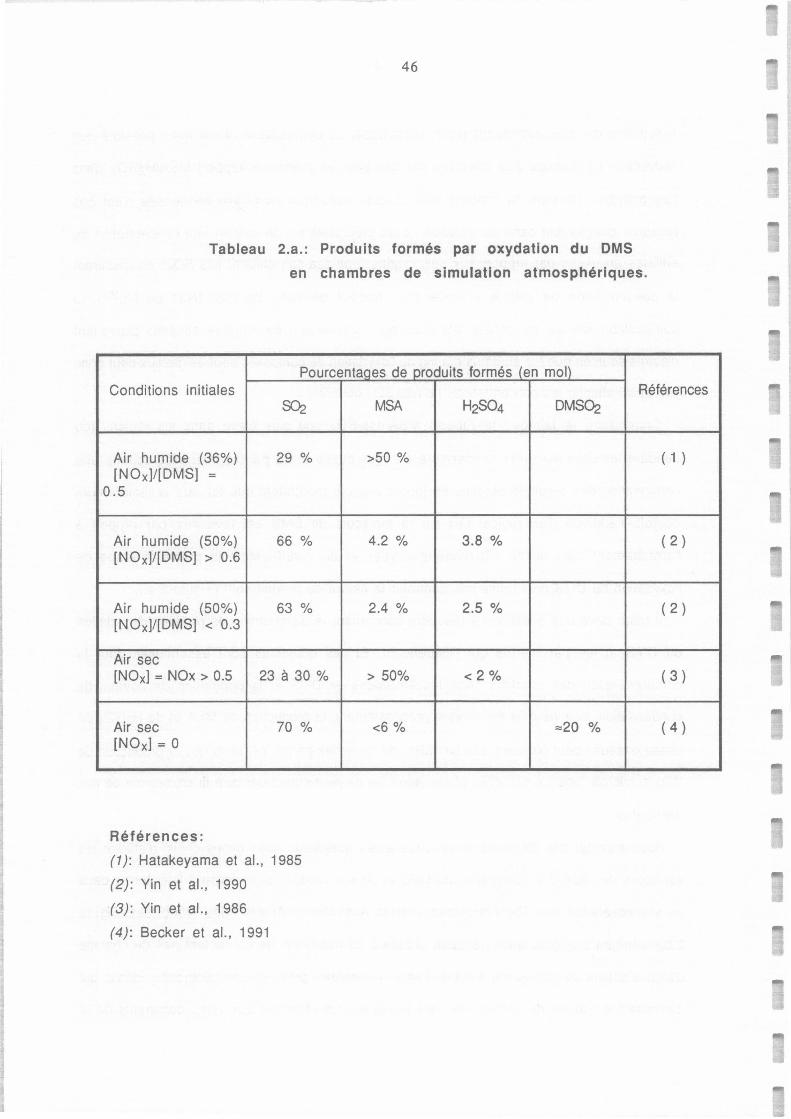
46
Tableau 2.a.: Produits formés par oxydation du OMS
en chambres de simulation atmosphériques.
Pourcentaaes de oroduits formés (en mol) Conditions initiales Références
~
Air humide (36%) 29 % [NOx]/[DMS] =
0.5
Air humide (50%) 66 % [NOx]/[DMS] > 0.6
Air humide (50%) 63 % [NOx]/[DMS] < 0.3
Air sec [NOx] = NOx > 0.5 23 à 30 %
Air sec 70 % [NOx] = 0
Références:
(1 ): Hatakeyama et al., 1985
(2): Yin et al., 1990
·(3): Yin et al., 1986
(4): Becker et al., 1991
MSA H2SO4 DMSÜ2
>50 % ( 1 )
4.2 % 3.8 % ( 2 )
2.4 % 2.5 % ( 2 )
> 50% <2% ( 3 )
<6 % ::::20 % ( 4 )
47
base par des sources de composés soufrés locales. De plus, son éloignement de près de 5000
km des continents habités et les conditions générales de circulation atmosphérique réduisent
la fréquence de contamination de l'atmosphère par transports à longue distance de polluants
anthropogéniques à quelques jours par an, identifiés grâce à l'enregistrement de l'activité du
Radon, traceur radioactif continental. L'intérêt de mesurer les concentrations de composés
soufrés à long terme (périodes d'observation >1 an) est d'obtenir des valeurs
représentatives de moyennes mensuelles qui peuvent être comparées malgré les pas de temps
de prélèvement différents selon les composés. Les moyennes mensuelles, lissant les
variations synoptiques, peuvent être interprétées en fonction des variations saisonnières de
paramètres climatiques (température, insolation). De plus, elles sont bien adaptées à la
validation de modèle globaux, également basés sur des moyennes mensuelles de flux
d'émissions et de transport des composés soufrés (e.g. Langner and Rhode, 1991, 1992)
Les travaux présentés dans ce chapitre concernent l'étude de la production de SO2, de MSA
et de H2SO4 à partir du DMS. Les mesures de OMS et de SO2 ont été effectuées à l'île
Amsterdam, respectivement par chromatographie en phase gazeuse (Nguyen et al., 1990) et
selon la méthode West-Gaeke modifiée par Nguyen et al. (1974). Les concentrations de MSA
et de sulfate en excès dans les précipitations ont été mesurées par chromatographie ionique
(Annexe 2), respectivement au Centre des Faibles Radioactivités à Gif-sur-Yvette et à
l'Université de Virginie (USA).
Les variations journalières et saisonnières de la concentration atmosphérique de SO2 sont
comparées avec celles du OMS. Un modèle de boîte photochimique est utilisé pour interpréter
les résultats obtenus.
Parallèlement, les variations de la concentration du MSA dans les précipitations et de son
flux par dépôt humide sont comparées avec les concentrations atmosphériques et le flux
océan atmosphère de OMS pour estimer la proportion de OMS oxydée en MSA. Il faut noter
qu 'afin que les valeurs présentées ici restent comparables avec celles de la littérature, les
valeurs de flux de OMS calculées dans les chapitres suivants à partir de la paramétrisation
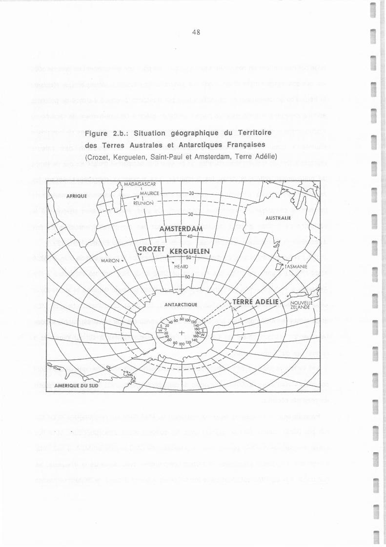
48
Figure 2.b.: Situation géographique du Territoire
des Terres Australes et Antarctiques Françaises
(Crozet, Kerguelen, Saint-Paul et Amsterdam, Terre Adélie)

49
de Liss et Merlivat (1986) n'ont pas été corrigées en tenant compte des résultats obtenus
dans le chapitre 1.
Enfin , les variations de concentrations des composés soufrés dans les précipitations sont
comparées à leur acidité afin d'y estimer la contribution des produits d'oxydation du OMS.
Ces résultats sont présentés dans les 3 articles suivants, rédigés simultanément,
complémentaires et nécessaires à l'interprétation des mesures présentées dans chacun
d'entre eux.
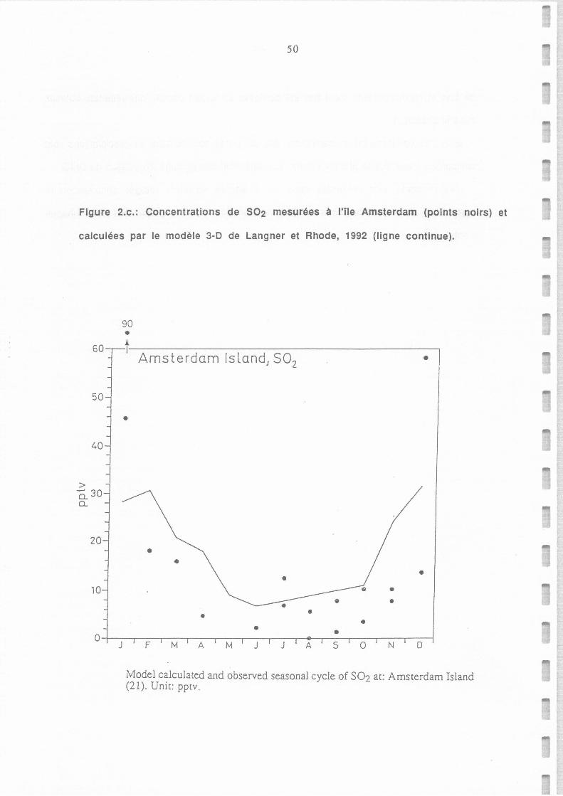
50
Figure 2.c.: Concentrations de S02 mesurées à l'île Amsterdam (points noirs) et
calculées par le modèle 3-D de Langner et Rhode, 1992 (ligne continue).
60
50
40
> ô_30 o.
20
10
0 J
90 • t-----------
Amsterdam Island) S02 •
•
•
• • • • • F M A M J J A s 0 N D
Mode! calculated and observed seasonal cycle of S02 at: Amsterdam Island (21). Unit: pptv.
51
Il.A. CONCENTRATIONS ATMOSPHERIQUES DE SULFURE DE DIMETHYLE ET DE
DIOXYDE DE SOUFRE EN MILIEU OCEANIQUE.
Le S02 est un produit intermédiaire du processus d'oxydation du OMS: il est
ultérieurement oxydé en acide sulfurique et joue donc un rôle central dans la chimie du OMS.
Du fait de son acidité et de sa grande réactivité en phase hétérogène, il est impossible de le
concentrer par piégeage cryogénique pour l'analyser par chromatographie en phase gazeuse à
l' instar du OMS: l'utilisation des moyens techniques qui seraient nécessaires ne peut être
envisagée dans les bases éloignées des circuits de distribution habituels de gaz liquéfiés,
entre autre. Nous avons donc mis en oeuvre une méthode spécifique, mise au point par
Nguyen et al. (1974) , qui nous a permis de mettre en évidence pour la première fois les
variations saisonnières de la concentration de S02. Ces mesures originales ont depuis
été utilisée à de nombreuses reprises pour valider des modèles globaux du cycle du soufre
(e.g . Langner and Rhode, 1992). De plus, elles constituent le "chaînon manquant" identifié
par Ayers et al. (1991) pour boucler le cycle liant le OMS, la concentration de ses produits
particulaires, et la population de CN et de CCN.
Dans l'article qui suit, les variations saisonnières de S02 sont interprétées grâce à
l'utilisation d'un modèle de boîte photochimique permettant d'obtenir une estimation de la
fraction de OMS oxydée en S02.

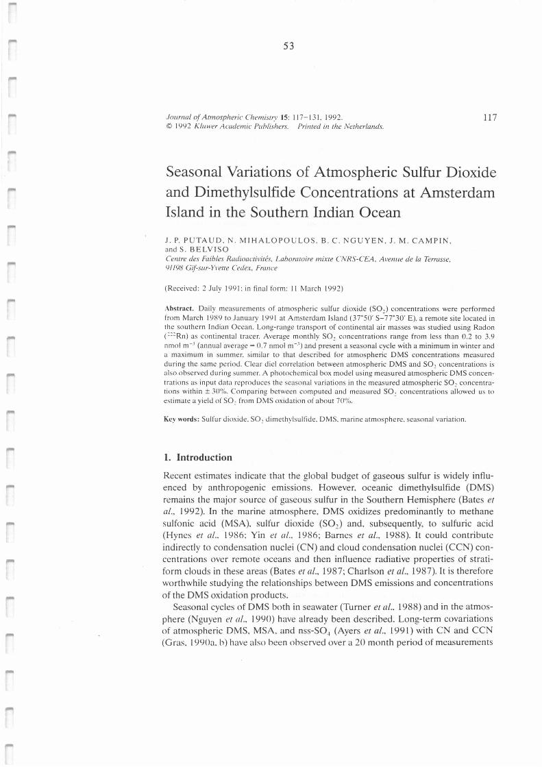
53
Jou ma/ of Atmospheric Chemis1ry 15: 11 7- 131. 1992. 117 © 1992 K/uwer Arndemic Puh/ishers. Pri111ed in the Ne1her/a11ds.
Seasonal Variations of Atmospheric Sulfur Dioxide and Dimethylsulfide Concentrations at Amsterdam Island in the Southern Indian Ocean
J. P. PUTAUD. N. MIHALOPOULOS . B. C. NGUYEN , J . M . CAMP I N. and S. BELVISO Ce111re des Faibles Radioac1ivilés. Labora1oire mix1e CNRS-CEA. Avenue de la Terrasse,
91198 Gifs11r-Y1-e11e Cedex. France
(Received: 2 July 199 1: in final form: 11 March 1992)
Abstract. Daily measurements of atmospheric sulfur dioxide (S0 2) concentrations were performed from March 1989 to January 1991 at Amsterdam Island (37°50' S-77°30' E). a remote si te located in the southe rn Ind ian Ocean. Long-range transport of continental air masses was studied using Radon ( 222 Rn) as continental tracer. Average monthly S0 2 concentrations range from less than 0.2 to 3.9 nmol m--' (annual average= 0.7 nmol m-3
) and present a seasonal cycle with a minimum in winter and a maximum in summer. similar to that described for atmospheric DMS concentrations measured during the same perioJ . Clear die! correlation between atmospheric DMS and S0 2 concentrations is also ohserved during summer. A photochemical box mode! using measured atmospheric DMS concen-trations as input data reproJuces the seasonal varia tions in the measured atmospheric S0 2 concentra-tio ns within ± 30%. Comparing between computed and measured S02 concentrations a llowed us to esti mate a yie lJ of S0 2 from DMS oxidation of about 70%.
Key words : Sulfur JioxiJe. S0 2 d imethylsullïde. DMS. marine atmosphe re. seasonal variation.
1. Introduction
Recent estimates indicate that the global budget of gaseous sulfur is widely influ-enced by anthropogenic emissions. However. oceanic dimethylsulfide (OMS) remains the major source of gaseous sulfur in the Southern Hemisphere (Bates et
al., 1992). In the marine atmosphere. OMS oxidizes predominantly to methane sulfonic acid (MSA). sulfur dioxide (SO~) and. subsequently, to sulfuric acid (Hynes et al.. 1986: Yin et al .. 1986; Barnes et al., 1988). It could contribute indirectly to condensation nuclei (CN) and cloud condensation nuclei (CCN) con-centrations over remote oceans and then influence radiative properties of strati-form clouds in these areas (Ba tes et al. , 1987; Charlson et al., 198 7). It is therefore worthwhile studying the re lationships between OMS emissions and concentrations of the OMS oxidation products.
Seasonal cycles of OMS both in seawater (Turner et al .. 1988) and in the atmos-phere (Nguyen et al .. 1990) have already been described. Long-term covariations of atmospheric OMS. MSA, and nss-SO ~ (Ayers et al .. 199 l) with CN and CCN (G ras. 1990a. b) have also been observed over a 20 month period of measurements
54
118 J. P. PUTAUD ET AL
performed at Cape Grim (41 • S, 144° E). But more extended series of measure-ments of SO2 are required to quantitatively understand the marine sulfur cycle. Indeed, only limited series of SO1 data are available for the Southern Hemisphere. The measurement performed on board oceanographic ships between 1974 and 1977 (n = 92) by Nguyen et al. (1983) described most of the subantarctic Indian Ocean but predominantly covered summer-fall (January-May). More recently, SO
1 concentrations have been measured for 2-4 week periods during a cruise
(Berresheim, 1987; Pszenny et al., 1989) and during one airborne experiment (Berresheim et al., 1990) without any attempt to deal with seasonal variations of atmospheric SO1 . Furthermore, simultaneous measurements of OMS and SO2 in remote areas (Andreae et al., 1988; Berresheim, 1987; Bates et al., 1990, Berres-heim et al., 1990) were too limited to show possible covariations of SO1 with OMS.
This paper presents the first 19 month series of SO1 measurements (recorded from March 1989 to January 1991) together with atmospheric OMS measured at the same place during the same period. Possible influence on the SO2 concentra-tions by long-range transport of anthropogenic pollutants is discussed subsequent to continuous monitoring with the continental tracer 111 Rn. Short-term variations of SO 1 and OMS are studied over four summer months. Seasonal variations of SO2
are discussed on the basis of average monthly concentrations and compared with the results of a photochemical box mode! using the measured atmospheric OMS concentrations as input data.
2. Experimental
Amsterdam Island (37°50' S. 77°30' E), located in the southern Indian Ocean about 3000 and 4500 km from the nearest lands upwind, Madagascar and southern Africa. respectively, is subjected to westerlies most of the time (Figure l ).
The only source of local pollution on this small island (55 km 2) is the generators supplying the 35-member base at ·Martin de Viviès·. To avoid contamination from the exhaust emissions of this engine which consumes 3 7 5 kg fuel a day, sampling was performed at 'Pointe Bénédicte', 2.5 km to the west of the base (Figure 1), in exclusively marine conditions (average daily wind direction out of the 60° -180° sector). Air was sampled from a 9 m high tower erected about 20 m from the cliff edge and 65 m above sea level.
Sulfur dioxide sampling was performed on a 24 hour basis, from 6.30 a.m. to 6.15 a.m., by using the West-Gaeke method (1956) modified by Nguyen et al.
( 1974 ). Oetails of the SO1 sampling and analysis methods and comparison with other analytical methods are given by Bonsang ( 1980). However, the West-Gaeke method was not among the analytical methods which were recently intercompared (Gregory et al., 1990). Uncertainties could affect the absolute value of the SO 1
mixing ratios, but the conclusions concerning relative changes in SO1 concentra-tions would not be affected by possible systematic errors due to the calibration of the analytical method.
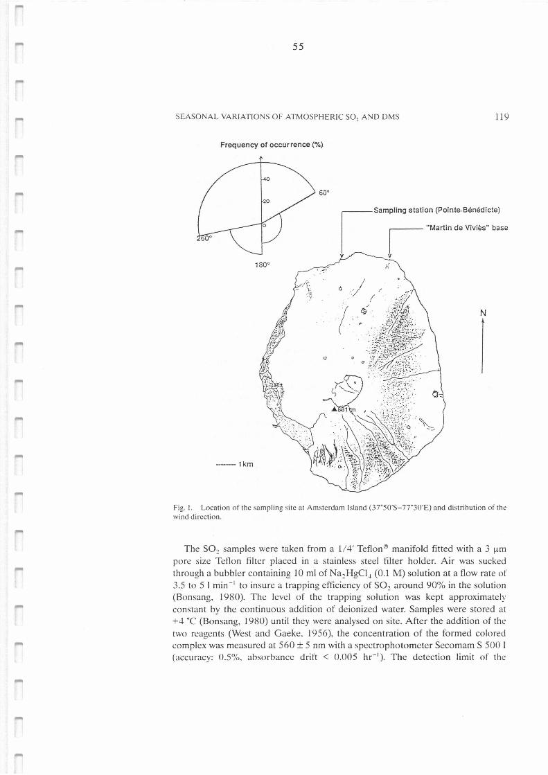
55
SEASONAL VARIATIONS OF ATMOSPHERIC SO, AND OMS 11 9
Frequency of occurrence(%)
40
so•
1ao 0
·- ' .:~~
----1km
[
Sampling station (Pointe,Bénédicte) l "Mart;n de VMès" base
'If V
à./ (
/
( -~ N
ô
Fig. 1. Location of the sampling site a t Amsterdam Island (37'50'S-77.30'E) and distribution of the wind direction.
The S0 2 samples were taken from a 1/4' Teflon® manifold fitted with a 3 µm pore size Teflon filter placed in a stainless steel filter holder. Air was sucked through a bubbler containing 10 ml of Na 2HgCl-1 (0.1 M) solution at a flow rate of 3.5 to 5 1 min - 1 to insure a trapping efficiency of S0 2 around 90% in the solution (Bonsang, 1980). The level of the trapping solution was kept approximately constant by the continuous addition of deionized water. Samples were stored at +4 °C (Bonsang, 1980) until they were analysed on site. After the addition of the two reagents (West and Gaeke, 1956), the concentration of the formed colored complex was measured at 560 ± 5 nm with a spectrophotometer Secomam S 500 I (accuracy: 0.5°/4,, absorbancc drift < 0.005 hr- 1 ). The detection limit of the
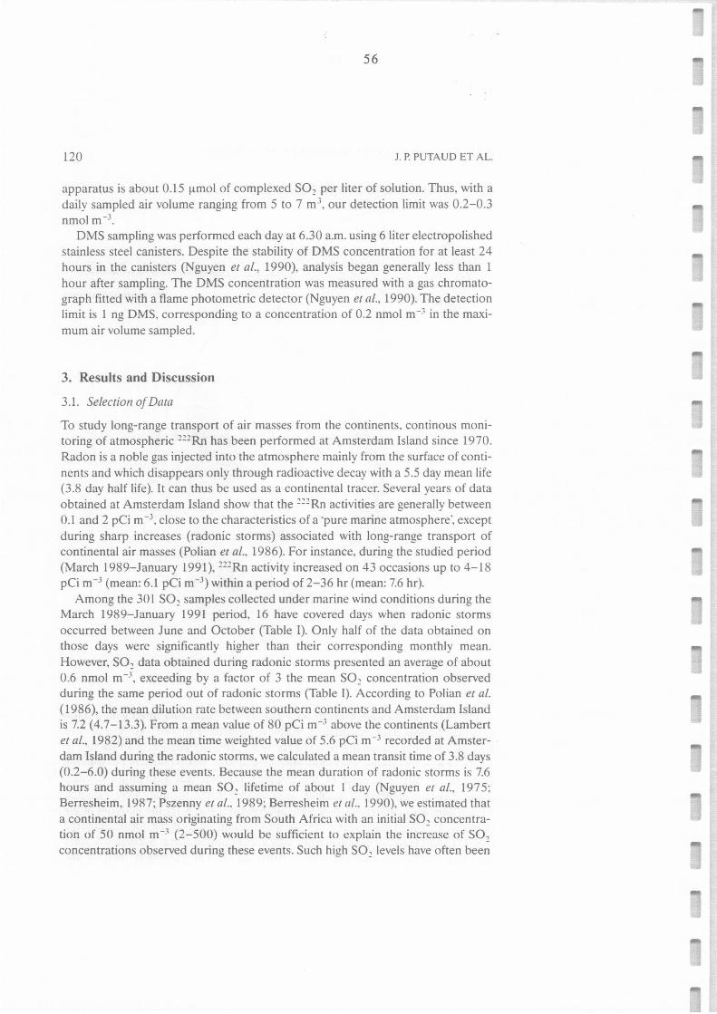
56
120 J. P. PUTAUD ET AL.
apparatus is about 0.15 µmol of complexed SO2 per liter of solution. Thus, with a daily sampled air volume ranging from 5 to 7 m 3
, our detection limit was 0.2-0.3 nmol m-3•
OMS sampling was performed each day at 6.30 a.m. using 6 liter electropolished stainless steel canisters. Oespite the stability of OMS concentration for at least 24 hours in the canisters (Nguyen et al., 1990), analysis began generally less than l hour after sampling. The OMS concentration was measured with a gas chromato-graph fitted with a flame photometric detector (Nguyen et al., 1990). The detection limit is 1 ng OMS, corresponding to a concentration of 0.2 nmol m-3 in the maxi-mum air volume sampled.
3. Results and Discussion
3.1. Selection of Data
To study long-range transport of air masses from the continents. continous moni-toring of atmospheric 222Rn has been performed at Amsterdam Island since 1970. Radon is a noble gas injected into the atmosphere mainly from the surface of conti-nents and which disappears only through radioactive decay with a 5.5 day mean life (3.8 day half life). It can thus be used as a continental tracer. Several years of data obtained at Amsterdam Island show that the 222 Rn activities are generally between 0.1 and 2 pCi m-3• close to the characteristics of a 'pure marine atmosphere·, except during sharp increases (radonic storms) associated with long-range transport of continental air masses (Polian et al., 1986). For instance, during the studied period (March 1989-January 1991), 222 Rn activity increased on 43 occasions up to 4-18 pCi m-3 (mean: 6.1 pCi m-3) within a period of 2-36 hr (mean: 7.6 hr).
Among the 301 SO2 samples collected under marine wind conditions during the March 1989-January 1991 period, 16 have covered days when radonic storms occurred between June and October (Table I). Only half of the data obtained on those days were significantly higher than their corresponding monthly mean. However, SO2 data obtained during radonic storms presented an average of about 0.6 nmol m--1_ exceeding by a factor of 3 the mean SO2 concentration observed during the same period out of radonic storms (Table l). According to Polian et al.
( 1986), the mean dilution rate between southern continents and Amsterdam Island is 7.2 (4.7-13.3). From a mean value of 80 pCi m-3 above the continents (Lambert et al., 1982) and the mean time weighted value of 5.6 pCi m-3 recorded at Amster-dam Island during the radonic storms, we calculated a mean transit time of 3.8 days (0.2-6.0) during these events. Because the mean duration of radonic storms is 7.6 heurs and assuming a mean SO 2 lifetime of about I day (Nguyen et al., 197 5; Berresheim, 1987; Pszenny et al .. 1989; Berresheim et al .. 1990), we estimated that a continental air mass originating from South Africa with an initial SO 2 concentra-tion of 50 nmol m-3 (2-500) would be sufficient to explain the increase of SO2
concentrations observed during these events. Such high SO2 levels have often been
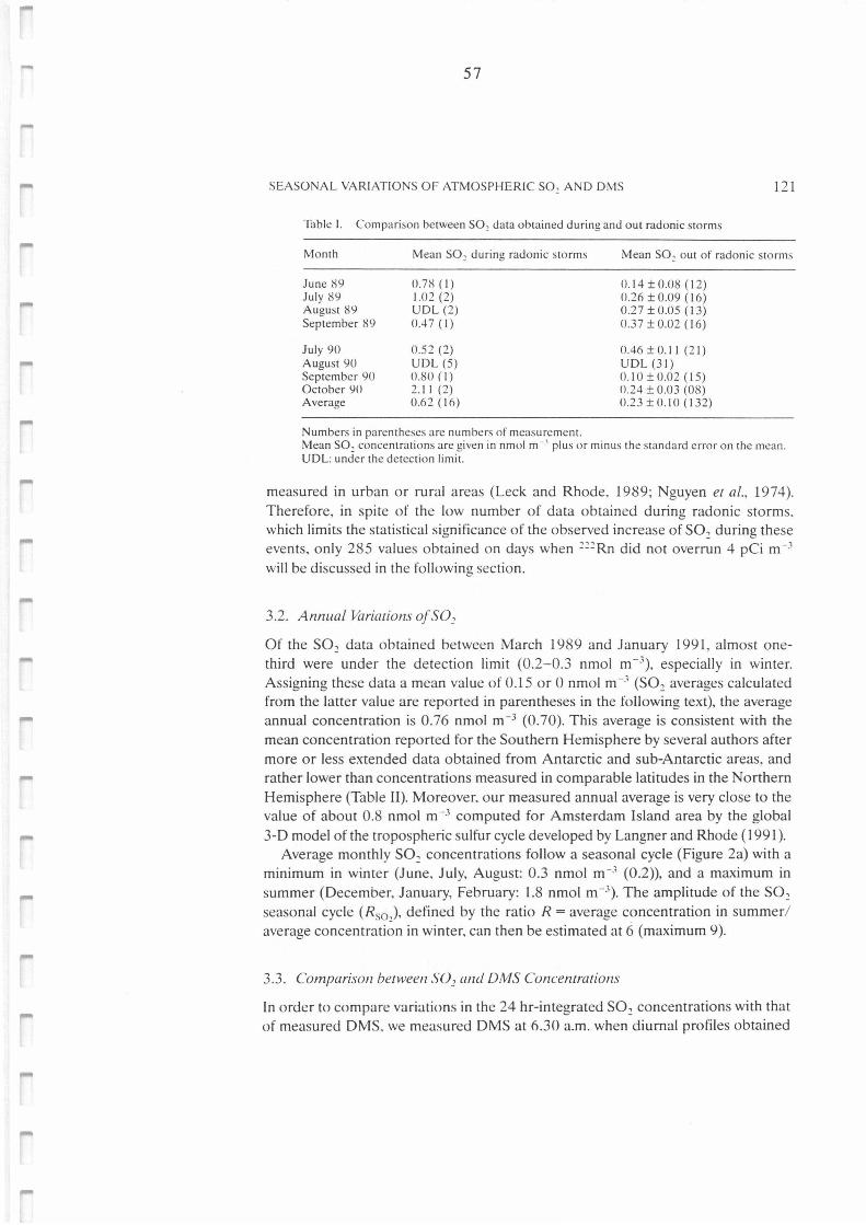
-57
SEASONAL VARIATIONS OF ATMOSPHERIC S0, AND OMS 121
Table l. Comparison between S0, data obtained during and out radonic storms
Month Mean SO: during radonic storms Mean SO, out of radonic storms
June 89 July 89 August 89 September 89
July 90 August 90 September 90 October 90 Average
0.78 ( 1) 1.02 (2) UDL (2) 0.47 (1)
0.52 (2) UDL (5) 0.80 (1) 2.11 (2) 0.62(16)
Numbers in parentheses are numbers of measurement.
0.14 ±0.08 (12) 0.26 ±0.09 (16) 0.27 ± 0.05 ( 13) 0.37 ±0.02 (16)
0.46 ± 0.1 1 (2 1) UDL (31) 0.10±0.02 (15) 0.24 ± 0.03 (08) 0.23±0.10(132)
Mean S0, concentrations are given in nmol m -3 plus or minus the standard erro r on the mean. UDL: under the detection limit.
measured in urban or rural areas (Leck and Rhode. 1989; Nguyen et al., 1974). Therefore, in spite of the low number of data obtained during radonic storms. which limits the statistical significance of the observed increase of S02 during these events. only 285 values obtained on days when 222 Rn did not overrun 4 pCi m-3
will be discussed in the following section.
3.2. Annual Variations of 502
Of the S0 2 data obtained between March 1989 and January 1991, almost one-third were under the detection limit (0.2-0.3 nmol m- 3). especially in winter. Assigning these data a mean value of 0.15 or O nmol m-3 (S0 2 averages calculated from the latter value are reported in parentheses in the following text), the average annual concentration is 0.76 nmol m-3 (0.70). This average is consistent with the mean concentration reported for the Southern Hemisphere by several authors after more or Iess extended data obtained from Antarctic and sub-Antarctic areas, and rather lower than concentrations measured in comparable latitudes in the Northern Hemisphere (Table II). Moreover. our measured annual average is very close to the value of about 0.8 nmol m -3 computed for Amsterdam Island area by the global 3-0 mode! of the tropospheric sulfur cycle developed by Langner and Rhode ( 1991 ).
Average monthly S0 2 concentrations follow a seasonal cycle (Figure 2a) with a minimum in winter (June. July, August: 0.3 nmol m-3 (0.2)), and a maximum in summer (Oecember, January, February: 1.8 nmol m-3). The amplitude of the S0 2
seasonal cycle (RsoJ, defined by the ratio R = average concentration in summer/ average concentrati;n in winter, can then be estimated at 6 (maximum 9).
3.3. Comparison between S02 and DMS Concentrations
ln order to compare variations in the 24 hr-integrated S0 2 concentrations with that of measured OMS. we measured OMS at 6.30 a.m. when diurnal profiles obtained
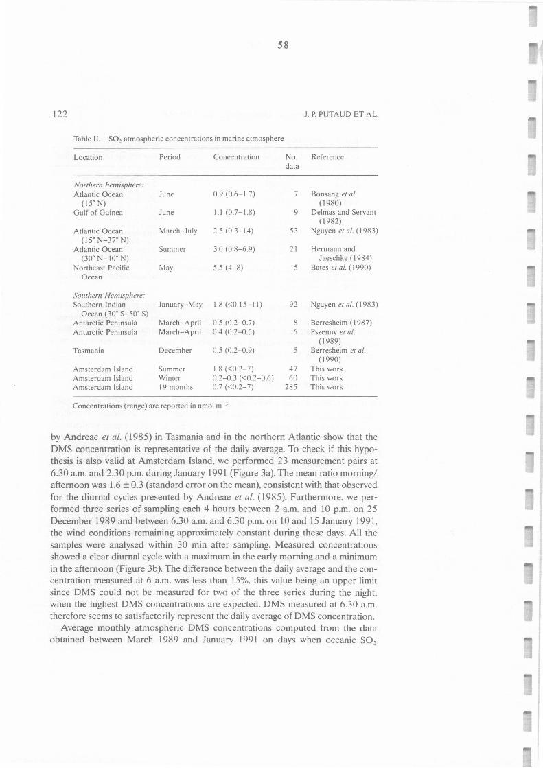
58
122 J. P. PUTAUD ET AL.
Table li. SO: atmospheric concentrations in marine atmosphere
Location Period Concentration No. Reference data
Northern hemisphere:
Atlantic Ocean June 0.9 (0.6-1.7) 7 Bonsang et al.
( 15° N) ( 1980) Gulf of Guinea June 1.1 (0.7-1.8) 9 Delmas and Servant
( 1982) Atlantic Ocean March-July 2.5 (0.3-14) 53 Nguyen et al. ( 1983)
( 15° N-37° N) Atlantic Ocean Summer 3.0 (0.8-6.9) 21 Hermann and
(30" N-40° N) Jaeschke (1984) Northeast Pacifie May 5.5 (4-8) 5 Bates et al. ( 1990)
Ocean
Southern Hemisphere:
Southern lndian January-May 1.8 (<0.15-11) 92 Nguyen et al. ( 1983) Ocean (30° S-50" S)
Antarctic Peninsula March-April 0.5 (0.2-0.7) 8 Berresheim ( 1987) Antarctic Peninsula March-April 0.4 (0.2-0.5) 6 Pszenny er al.
(1989) Tasmania Deœmber 0.5 (0.2-0.9) 5 Berresheim et al.
( 1990) Amsterdam Island Summer 1.8 ( <0.2-7) 47 This work Amsterdam Island Winter 0.2-0.3 (<0.2-0.6) 60 This work Amsterdam Island 19 months 0.7 (<0.2-7) 285 This work
Concentrations (range) are reported in nmol m--'.
by Andreae et al. ( 1985) in Tasmania and in the northern Atlantic show that the OMS concentration is representative of the daily average. To check if this hypo-thesis is also valid at Amsterdam Island, we performed 23 measurement pairs at 6.30 a.m. and 2.30 p.m. during January 1991 (Figure 3a). The mean ratio morning/ afternoon was 1.6 ± 0.3 (standard error on the mean), consistent with that observed for the diurnal cycles presented by Andreae et al. (1985). Furthermore. we per-formed three series of sampling each 4 hours between 2 a.m. and 10 p.m. on 25 Oecember 1989 and between 6.30 a.m. and 6.30 p.m. on 10 and 15 January 1991. the wind conditions remaining approximately constant during these days. Ali the samples were analysed within 30 min after sampling. Measured concentrations showed a clear diurnal cycle with a maximum in the early morning and a minimum in the afternoon (Figure 3b). The difference between the daily average and the con-centration measured at 6 a.m. was less than 15%. this value being an upper limit since OMS could not be measured for two of the three series during the night. when the highest OMS concentrations are expected. OMS measured at 6.30 a.m. therefore seems to satisfactorily represent the daily average of OMS concentration.
Average monthly atmospheric OMS concentrations computed from the data obtained between March 1989 and January 1991 on days when oceanic SO2
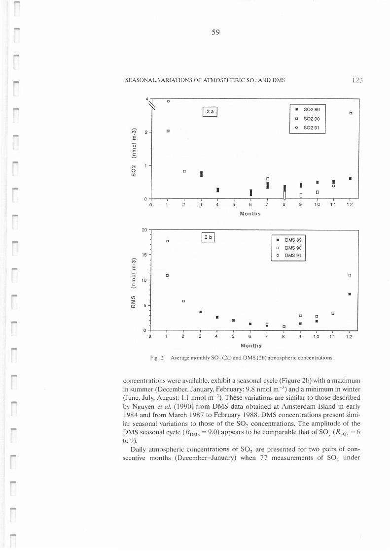
59
SEASONAL VARIATIONS OF ATMOSPHERIC SO, AND OMS 123
4 ---0--------------------------~
'; 2 E 0
E C
N
0 en
C
C 1
1
a 1
1
• SO2 89
c SO2 90
o SO2 91
• a
1 C
C
• 1
0 0 -+--~-----.------,-----.---..----,----u-~------,-----.----' 0 2 3 4 5 6
Months
7 8 9 1 0 11 12
20 -r-----------------------------~
15
M
E 0 E 10
.s en :E Cl 5
0
C
C
• • • •
• OMS 89
c OMS 90
o OMS 91
C
C
• C
•
C
•
0 -t----r-----.--~---,-----.---..----,-----,---,-------,-----' 0 2 3 4 5 6
Months
7 8 9 1 0 11
Fig. 2. Average monthly SO, (2a) and OMS (2b) atmosp heric concentrations.
12
concentrations were available, exhibit a seasonal cycle (Figure 2b) with a maximum in summer (Oecember. January, February: 9.8 nmol m-3) and a minimum in winter (June, July, August: 1.1 nmol m-3). These variations are similar to those described by Nguyen er al. ( 1990) from OMS data obtained at Amsterdam Island in early 1984 and from March 1987 to February 1988. OMS concentrations present simi-lar seasonal variations to those of the S02 concentrations. The amplitude of the OMS seasonal cycle (RDMs = 9.0) appears to be comparable that of S0 2 (Rso
2 = 6
to 9). Oaily atmospheric concentrations of S0 2 are presented for two pairs of con-
secutive months (Oecember-January) when 77 measurements of SO~ under
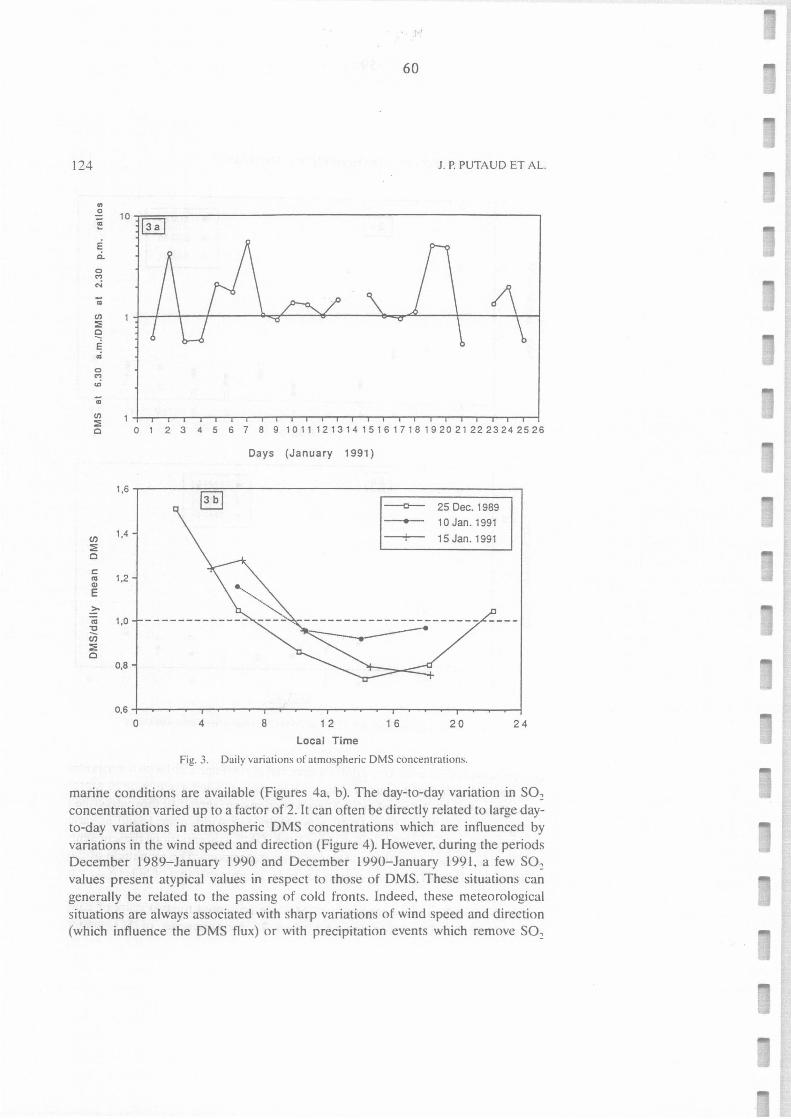
124
., 0
~
Ë ci.
0 "! "' ai (/)
::E e Ë .;
0 <"! .,,
ai (/)
::E 0
(f)
:!: Cl
C:
"' Q)
E
~
"' "C
èn :!: Cl
60
J. P. PUTAUD ET AL.
10 r:;71 ~
1,6
1,4
1,2
1,0
0,8
0,6
O 1 2 3 4 5 6 7 8 9 1011121314151617181920212223242526
Days (January 1991)
0 4 8 1 2
Local Time
--o-- 25 Dec. 1989
-- 10Jan.1991
-+- 15 Jan. 1991
1 6 20
Fig. 3. Daily variations of atmospheric DMS concentrations.
24
marine conditions are available (Figures 4a, b ). The day-to-day variation in SO, concentration varied up to a factor of 2. It can often be directly related to large day-to-day variations in atmospheric OMS concentrations which are intluenced by variations in the wind speed and direction (Figure 4 ). However. during the periods December 1989-January 1990 and Oecember 1990-January 1991, a few Sû:! values present atypical values in respect to those of OMS. These situations can generally be related to the passing of cold fronts. Indeed, these meteorological situations are always associated with sharp variations of wind speed and direction (which influence the OMS flux) or with precipitation events which remove SO,
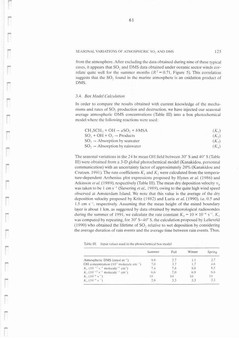
61
SEASONAL VARIATIONS OF ATMOSPHERIC SO, AND DMS 125
from the atmosphere. After excluding the data obtained during nine of these typical cases, it appears that SO2 and OMS data obtained under oceanic sector winds cor-relate qui te well for the summer months (R 2 = 0.71 , Figure 5). This correlation suggests that the S0 2 found in the marine atmosphere is an oxidation product of OMS.
3.4. Box 1\llodel Calculation
In order to compare the results obtained with current knowledge of the mecha-
nisms and rates of S0 2 production and destruction, we have injected our seasonal average atmospheric OMS concentrations (Table III) into a box photochemical mode! where the following reactions were used:
CH 3SCH 3 + OH - aSO2 + bMSA
SO, +OH+ 0, - Products - -S0 2 - Absorption by seawater SO 2 - Absorption by rainwater
(K1) (KJ
(K _,)
(K.i)
The seasonal variations in the 24 hr mean OH field between 30° Sand 40° S (Table III) were obtained from a 3-0 global photochemical mode! (Kanakidou. personnal communication) with an uncertainty factor of approximately 20% (Kanakidou and Crutzen. 1991 ). The rate coefficients K I and K 2 were calculated from the tempera-ture-dependent Arrhenius plot expressions proposed by Hynes et al. (1986) and Atkinson et al. ( 1989), respectively (Table III). The mean dry deposition velocity vJ was taken to be 1 cm S- 1 (Sievering et al.. 1989), owing to the quite high wind speed observed at Amsterdam Island. We note that this value is the average of the dry deposition velocity proposed by Kritz ( 1982) and Luria et al. ( 1990). i.e. 0.5 and 1.5 cm ç 1
• respectively. Assuming that the mean height of the mixed boundary layer is about 1 km, as suggested by data obtained by meteorological radiosondes during the summer of 1991 , we calculate the rate constant K 3 = 10 x 10-6 Ç 1• K.i
was computed by repeating, for 30° S-40° S. the calculation proposed by Lelieveld ( l 990) who obtained the lifetime of S0 2 relative to wet deposition by considering the average duration of rain events and the average time between rain events. Thus.
Table III. Input va lues usecJ in the photochemical hnx mocJel
Atmospheric DMS (nmol m ·' ) OH concentration ( 1 () ' molccule cm - ' ) "- 1 (10- 12 s - ' molecule - 1 cm ·' ) "- : ( 10- 1
: s - 1 molecuk - 1 cm 3J /.:. , (10-" s - 1)
"J (10-" s 1
)
Summer Fall
9.8
7.0 7.-4 (1.(1
Ill
2.7
J.7 7.8 7.0
!il
Winter Spring
1.1 2.7
1.7 -4.6 8.8 8.5 6.9 6.8
10 10
3.3 3.3
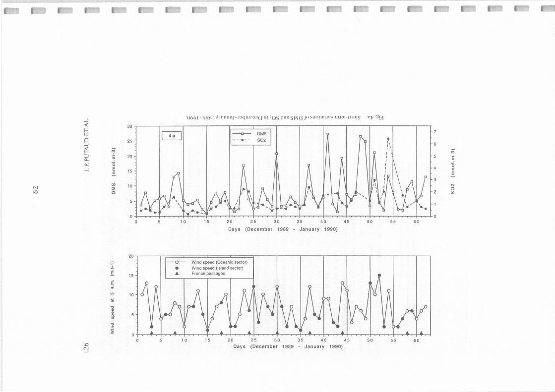
_j "0661-MU, 1 AJl!lllll!("- J:lqtu:i:i:ic1 lll · os pun Sl"JCI JO SUOlll!IJI?,\ lUJ:ll-lJ<HIS ·nt, ·fh:.J
~ 30 f-UJ
25 J 1~ Cl ::> ~ '? ::> c... E 20
--0-- OMS 1 1 1 lî 1 f\, 1
1 1 r7 ---- S02 • •• 6 ,, 1 1
M 1 1 5 È 1
o.; 0 -; E
5 15
N (/)
\0 :;; 10
0
5
1 1 0 1 1 4 E 1 1 1 1
C
! -r 1 3
,. 1 \(\ N , 1 1 0
~ 1 ' 2
', I (/)
.,_ I
• 0
5 10 15 20 25 30 35 40 45 50 55 60
Days (December 1989 - January 1990)
20
~ -0-- Wind speed (Oceanic sector)
' ., i 15
• Wind speed (Island seclor) A Frontal passages
È .;
"' 10
• ..., ., 5
., Q. ., ..., C
§: 0
0 5 10 15 20 25 30 35 40 45 50 55 60 \Cl N Days (December 1989 - January 1990)
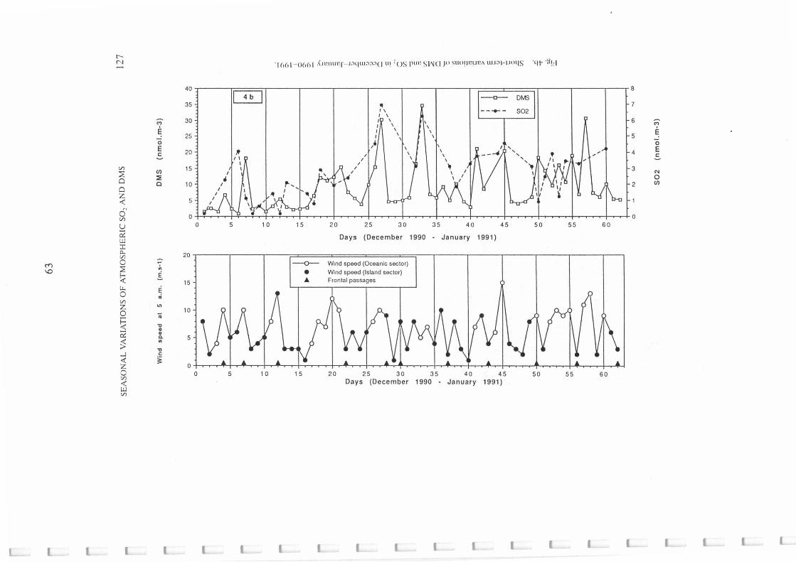
r--N · 1 c,c, 1- 06(, 1 ,\JIHllll? f - J:>qLU;):l;)(l lll 'os pt11? SI/\JCI JO SllO!)l?IJlli\ lU.l;}l-1.IOl)S ·qp ·;h:_1
:: ] 1~1 1 1 1 ~ 1 0 1 1 1~ D~ Il 1 1 C SO2
M 30 \ \ 6 M \
è \ \ è \
25 \ \ 5 \ 0
\ 0 E \ E 20 ,,
\ \ ... 4 C \ ... .s ~ '] \ \ ... V) 15 • 3 ~
en I 1 I N
::E 4 \ I I 0
0 Cl 10 I ,....,
n tl 2 en 0 z <l'. 5
o' 0 - - - - 0 V)
u 0 5 1 0 15 20 25 30 35 40 45 50 55 60
ë2 Days (December 1990 . January 1991) UJ :r: o.. 20 V)
~ 0 ~
1J 1 1 1: Wind speed (Oceanic seclor) \0 ~ ..
Wind speed (Island sector) \;;: g
Frontal passages W.. E 0 ,; V)
z 1/)
0 10
~ ï. .,, .,
ë2 ., Il. 5
~ Ill
.,, .J C
<l'. §: z 0 0 5 1 0 1 5 20 25 30 35 40 45 50 55 60 V)
Days (December 1990 January 1991) <l'. . IJJ V)
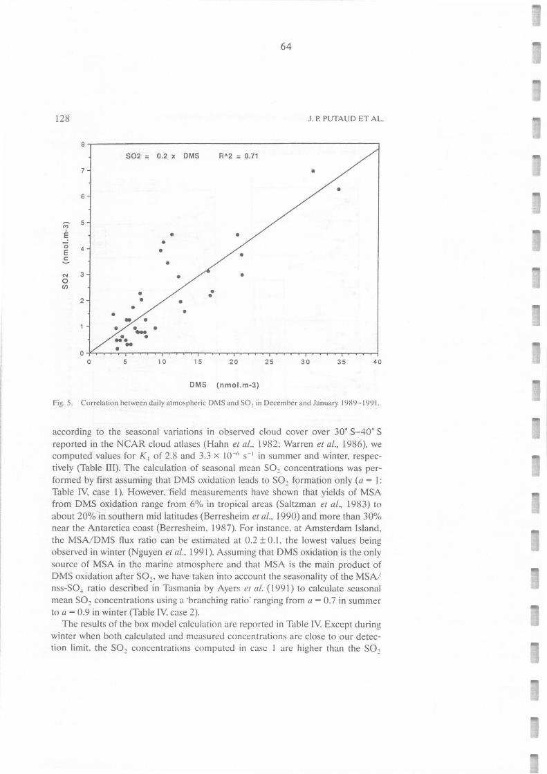
128
8
7
6
.., 5
è _; 0 4 E C:
N 3 0 (/)
2
•
0
SO2 = 0.2 x DMS R"2 = 0.71
5
• •
•
• •
•
10
•
•
15
• •
•
20
DMS (nmol.m-3)
64
J. P. PUTAUD ET AL.
•
25 30 35 40
Fig. 5. Correlation hetween daily atmospheric OMS and SO~ in December and January 1989-1991.
according to the seasonal vanattons in observed cloud cover over 30° S-40° S reported in the NCAR cloud atlases (Hahn et al .. 1982: Warren et al., 1986), we computed values for K4 of 2.8 and 3.3 x 10-r, ç 1 in summer and winter, respec-tively (Table III). The calculation of seasonal mean S0 2 concentrations was per-formed by first assuming that OMS oxidation leads to S0 2 formation only (a= l: Table IV, case l ). However, field measurements have shown that yields of MSA from OMS oxidation range from 6% in tropical areas (Saltzman et al., 1983) to about 20% in southern mid latitudes (Berresheim et al., 1990) and more than 30% near the Antarctica coast (Berresheim, 1987). For instance. at Amsterdam Island. the MSA/OMS flux ratio can be estimated at 0.2 ± 0.1, the lowest values being observed in winter (Nguyen et al .. 1991 ). Assuming that OMS oxidation is the only source of MSA in the marine atmosphere and that MSA is the main product of OMS oxidation after S0 2, we have taken into account the seasonality of the MSA/ nss-SO4 ratio described in Tasmania by Ayers et al. ( I 991) to calculate seasonal mean S0 2 concentrations using a 'branching ratio· ranging from a= 0.7 in summer to a= 0.9 in winter (Table IV. case 2).
The results of the box model calculation are reported in Table IV. Except during winter when both calculated and measured concentrations are close to our detec-tion limit, the S0 2 concentrations computed in case I are higher than the S0
2
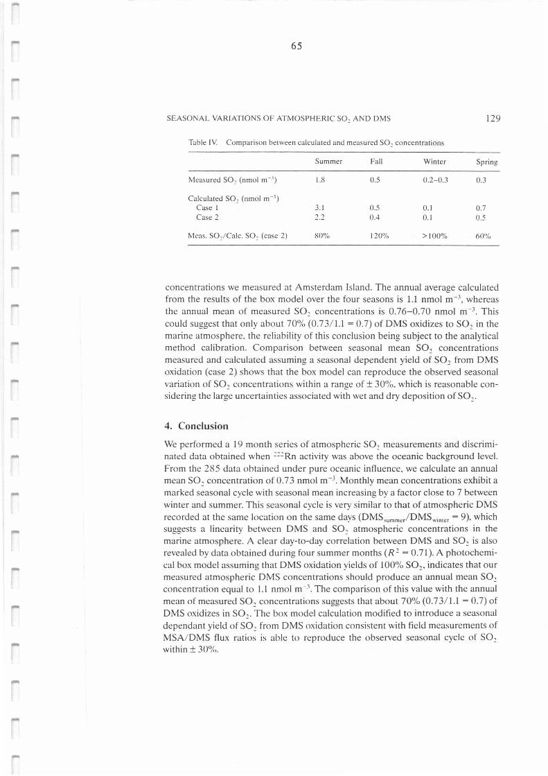
65
SEASONAL VARIATIONS OF ATMOSPHERIC SO, AND DMS 129
Table IV Comparison between calculated and measured SOè concentrations
Summer Fall Winter Spring
Measured SO 2 (nmol m-3) 1.8 0.5 0.2-0.3 0.3
Calculated SO2 (nmol m- ') Case 1 3.1 0.5 0.1 0.7 Case 2 2.2 0.4 0.1 0.5
Meas. SO/ Calc. SO: (case 2) 80% 120% > 100% 60%
concentrations we measured at Amsterdam Island. The annual average calculated from the results of the box mode! over the four seasons is 1.1 nmol m-3, whereas the annual mean of measured S0 2 concentrations is 0.76-0.70 nmol m- 3_ This
could suggest that only about 70% (0.73/ 1.1 = 0.7) of DMS oxidizes to S02 in the marine atmosphere. the reliability of this conclusion being subject to the analytical method calibration. Comparison between seasonal mean S02 concentrations measured and calculated assuming a seasonal dependent yield of S02 from DMS oxidation (case 2) shows that the box mode! can reproduce the observed seasonal variation of S0 2 concentrations within a range of± 30%. which is reasonable con-sidering the large uncertainties associated with wet and dry deposition of S0 2 •
4. Conclusion
We performed a 19 month series of atmospheric S0 2 measurements and discrimi-nated data obtained when 222 Rn activity was above the oceanic background level. From the 285 data obtained under pure oceanic influence, we calculate an annual mean S0 2 concentration of 0.73 nmol m-3. Monthly mean concentrations exhibit a marked seasonal cyc le with seasonal mean increasing by a factor close to 7 between winter and summer. This seasonal cycle is very similar to that of atmospheric DMS recorded at the same location on the same days (DMS,umme/DMSwinter = 9), which suggests a linearity between DMS and S0 2 atmospheric concentrations in the marine atmosphere. A clear day-to-day correlation between DMS and S0 2 is also revealed by data obtained during four summer months (R 2 = 0.71). A photochemi-cal box mode! assuming that DMS oxidation yields of 100% S0 2 , indicates that our measured atmospheric DMS concentrations should produce an annual mean S0 2
concentration equal to l.l nmol m-:1_ The comparison of this value with the annual mean of measured S0 2 concentrations suggests that about 70% (0.73/1.l = 0.7) of DMS oxidizes in SO,. The box mode! calculation modified to introduce a seasonal dependant yield of S0 2 from DMS oxidation consistent with field measurements of MSA/ DMS flux ratios is able to reproduce the observed seasonal cycle of S0 2
within ± 30%.
66
130 J. P. PUTAUD ET AL.
Acknowledgements
We thank A. Gaudry, organizer of the Laboratory of Atmospheric Chemistry of Amsterdam Island for fruitful collaboration, B. Ardouin and G. Polian for pro-viding radon data. M. Kanakidou, J. Langner. J. Lelieveld, G. Lambert, J. C. Duplessy, C. Laj, and A. McTaggart for helpful discussions and comments and C. Harris for her help in preparing this manuscript. This work was supported by the Territoire des Terres Australes et Antarctiques Françaises. the Centre National de la Recherche Scientifique. and the Commissariat à l'Energie Atomique. This is CFR contribution No. 1250.
References
Andreae. M. O., Ferek. R. J .. Bermond. F., Byrd. K. P.. Engstrom. R. T.. Hardin. S., Houmere. P. D .. LeMarrec, F.. Raemdonck. H .. and Chatfield. R. B .. 1985. Dimethylsulfide in the marine atmos-phere. J. Geophys. Res. 90. 12891-12900.
Andreae. M. O., Berresheim. H .. Andreae. T. W.. Kritz. M. A.. Bates. T. S .. and Merri!!. J. T .. 1988, Vertical distribution of dimethylsulfide. sulfur dioxide. aerosol ions. and radon over the northeast Pacifie Ocean. J. Atmos. Clzem. 6. 149-173.
Atkinson. R.. Baulch. D. L.. Cox. R. A.. Hampson. R. F. Jr .. Kerr. J. A.. and Troe. J .. 1989. Evaluated kinetic and photochemical data for atmospheric chemistry: supplement lll. J. Ph1·s. Chem. Data 18. 881-1097.
Ayers. G. P .. lvey, J. P .. and Gillett. R. W .. 1991 , Coherence hetween seasonal cycles of dimethyl sul-phide. methanesulphonate and sulphate in marine air. Nawre 349. 404-406.
Barnes. 1.. Bastian, V.. and Becker. K. H .. 1988. Kinetics and mechanisms of the reaction of OH radi-cals with dimethyl sulfide. /111. J. C/zem. Kin. 19. 489-501.
Bates. T. M., Cline. J. D .. Gammon. R. H .. and Kelly-Hansen. S. R .. 1987. Regional and seasonal varia-tion of the flux of oceanic dimethylsulfide to the atmosphere. J. Geoplzys. Res. 92. 2930-2938.
Bates. T. S .. Johnson. J. E .. Quinn. P. K.. Goldman. P. D .. Kuster. W.C.. Covert. D. C.. and Hahn. C. J .. 1990. The biogeochemical sulfur cycle in the marine boundary layer over the northeast Pacifie Ocean. J. Atmos. Clzem. 10. 59-81.
Bates. T. S .. Lamb. B. K .. Guenther. A. B .. Oignon. J .. and Stoiber. E. S .. 1992. Sulfur emissions to the atmosphere from natural sources. J. Almos. Chem. 14. 315-337.
Berresheim. H .. 1987. Biogenic sulfur emission from the subantarctic and Antarctic Oceans. J. Geo-
phys. Res. 92, 13245-13262. Berresheim. H., Andreae. M. O .. Ayers. G. P .. Gillett. R. W.. Merrill. J. T .. Davis. V. J .. and Chameides.
W. L.. 1990, Airborne measurements of dimethylsulfide. sulfur dioxide. and aerosol ions over the Southern Ocean south of Australia. J. Almos. Chem. 10. 341-370.
Bonsang. B., 1980, Cycle atmosphérique du soufre d"origine marine. PhD Thesis. Université de Picardie.
Bonsang. B., Nguyen. B. C.. Gaudry. A .. and Lambert. G .. 1980. Sulfate enrichment in marine aerosols owing to biogenic gaseous sulfur compounds. J. Geophys. Res. 85. 7410-7416.
Charlson. R. J .• Lovelock. J. E .. Andreae. M. O .. and Warren. S. G .. 1987. Oceanic phytoplankton. atmospheric sulphur. cloud albedo and climate, Nawre 326. 655-661.
Delmas. R. and Servant. J .. l 982. The origin of sulfur compounds in the atmosphere of a zone of high productivity (Gulf of Guinea). J. Gr>oplzys. Res. 87, l l O l 9-1 l 026.
Gras, J. L.. 1990a. Baseline atmospheric condensation nuclei at Cape Grim 1977-1987. J. Atmos.
Chem. Il. 89-106. Gras. J. L.. l 990h, Cloud condc:nsation nucki over the southcrn occan. Grnp/zys. Res. Leu. 17. 1565-
1567. Gregory. G. l., Hoel. J. M. Jr .. and Davis. D. D .. 1990. Airhornc sulfur trace spccies intercomparison
campaign: sulfur dioxidc:. dimc:thylsulfide. hydrogen sulfidc. carhon disultidc and carhonyl sultïde. paper presented at the AGU Fall meeting. San Francisco. U.S.A .. Dccemher 3-7.
67
SEASONAL VARIATIONS OF ATMOSPHERIC S0 2 AND OMS 131
Hahn. C. J .. Warren. S. G .. Lo ndon. J .. Chervin. R. M .. and Jenne. R. L., 1982, Atlas of simultaneous occurrence of different cloud types amount over the ocean. NCAR Technical Note TN-201 + STR. Boulder. Co.
Hermann. J . and Jaeschke. W.. 1984. Measurements of H ,S and S0 2 over the Atlantic Ocean. J.
Atmos. Chem. 1. 111-123.
Hynes. A. J .. Wine. P. H., and Semmes. D. H .. 1986. Kinetics and mechanisms of OH reactions with organic sulfides, J. Phys. Chem. 90. 4148-4156.
Kanakidou, M .. and Crutzen. P.J .. 1991. Scale problems in global tropospheric chemistry modelling: comparison of results obtained with 3D mode!. adopting longitudinally uniform and varying emis-sions of NO, and NMHC. submitted to Chemosphere.
Kritz. M. A .. 1982. Exchange of sulfur between the free troposphere. marine boundary layer and the sea surface. J. Ceophys. Res. 87. 8795-8803.
Lambert. G .. Polian. G .. Sanak. J .. Ardouin. B .. Buisson. A.. Jégou. A.. and Le Roulley. J. C.. 198 2. Radon and daughter products cycle: application to troposphere-stratosphere exchanges. A1111.
Géophys. 38. 497-531.
Langner. J. and Rhode. H .. 1991. A global three-d imensiona l mode! of the tropospheric sulfur cycle. J.
Armas. Chem. 13. 225-263. Leck. C. and Rhode. H .. 1989. On the relation between anthropogenic SO, emissions and concentra-
tions of sulfate in air and precipitation. Atmos. E11viro11. 23. 959-966. Lelieveld. J .. 1990. The role of clouds in tropospheric photochemistry. PhD Thesis. University of
Utrecht.
Luria. M .. Van Valin. C. C.. Gunter. R. L.. Wellman. D. L.. Keene. W.C.. Galloway. J . N .. Sievering. H .. and Boatman. J. F.. 1990. Sulfur dioxide over the North Atlantic Ocean during GCE/ CASE/ WATOX. Global Biogeochem. Cycles 4. 381-393.
Nguyen. B. C.. Bonsang. B .. and Lambert. G .. 1974. The atmospheric concentration of sulfur dioxide
and sulfate aerosol over antarctic. subantarctic areas and ocean. Tel/us 26. 241-24 7. Nguyen. B. C.. Bonsang. B .. Lambert. G .. and Pasquier. J . L.. 1975. Residence time of the sulfur
dioxide in the marine atmosphere. Pure Appt. Ceophys. 123. 489-500. Nguyen. B. C.. Bonsang. B .. and Gaudry. A .. 1983. The role of the ocean in the global atmospheric
sulfur cycle. J. Ceophys. Res. 88. 10903-10914. Nguyen. B. C.. Mihalopoulos. N .. and Belviso. S .. 1990. Seasonal variation of atmospheric OMS at
Amsterdam Island in the Southern lndian Ocean. J. A{lnos. Chem. li. 123-141. Nguyen. B. C.. Gallet. L.. Mihalopoulos. N .. Putaud. J. P .. and Belviso. S .. 1991. Seasonal variation of
OMS and MSA at Amsterdam Island in the southern Indian Ocean. paper presented at the Euro-pean Geophysical Society XVI General Assembly. Wiesbaden. FRG. April 22-27.
Polian. G .. Lambert. G .. Ardouin. B .. and Jégou. A.. 1986. Long range transport of continental radon in subantarctic areas. Tel/us 38B. l 78-189.
Pszenny. A. A. P .. Castelle. A. J.. and Galloway. J. N .. l 989. A study of sulfur cycle in the Antarctic marine houndary layer. J. Gt'ophys. Res. 94. 9818-9830.
Saltzman. E. S .. Savoie. D. L.. Zika. R. G .. and Prospero. J . M .. 1983. Methane sulfonic acid in the marine atmosphere. J. Gt!ophys. Res. 88. 10897-10902.
Sievering. H .. Boatman. J.F.. Luria. M .. and Van Valin. R. L., 1989. Sulfur dry deposition over the North Atlantic: the role of coarse aerosol particles. Tel/us 41B. 338-343.
Turner. S. M .. Malin. G .. Liss. P. S .. Harbour. D. S .. and Holligan, P. M .. 1988. The seasonal variation of dimethylsultïde and dimethylsulfoniopropionate concentrations in nearshore waters. Li11111u/.
Ucc:a11ogr. 33. 364-37 .5. Warren. S. G .. Hahn. C. J .. Lnndon. J .. Chervin. R.. and Jenne. R. L.. l 986, Global of total cloud cover
and cloud type amount ovcr land. NCAR Tcchnical Note TN-273 + STR. Boulder. Co. West. P. W. and Gaeke. G. C.. 1956. Fixation of sulfur dioxide as disullïtomercurate (Il) and suhse-
quent colorimctric estimation. A11a/wirn/ Ch!'m. 28. 1816-1819. Yin. F.. Grosjean. D .. and Seinfdd. J.H .. l 986. Analysis of atmospheric photooxidation mechanisms
for nrganosulfur compoumh. J. (ieophys. /?es. 91. 14417-14438.

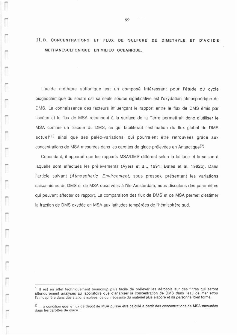
69
IL B. CONCENTRATIONS ET FLUX DE SULFURE DE Dl METHYLE ET D'ACIDE
METHANESULFONIOUE EN MILIEU OCEANIQUE.
L'acide méthane sulfonique est un composé intéressant pour l'étude du cycle
biogéochimique du soufre car sa seule source significative est l'oxydation atmosphérique du
OMS. La connaissance des facteurs influençant le rapport entre le flux de OMS émis par
l'océan et le flux de MSA retombant à la surface de la Terre permettrait donc d'utiliser le
MSA comme un traceur du DMS, ce qui faciliterait l'estimation du flux global de DMS
actuel( 1 l ainsi que ses palée-variations, qui pourraient être retrouvées grâce aux
concentrations de MSA mesurées dans les carottes de glace prélevées en Antarctique(2)_
Cependant, il apparaît que les rapports MSNDMS diffèrent selon la latitude et la saison à
laquelle sont effectués les prélèvements (Ayers et al., 1991; Bates et al, 1992b). Dans
l'article suivant (Atmospheric Environment, sous presse), présentant les variations
saisonnières de DMS et de MSA observées à l'île Amsterdam, nous discutons des paramètres
qui peuvent affecter ce rapport. La comparaison des flux de DMS et de MSA permet d'estimer
la fraction de DMS oxydée en MSA aux latitudes tempérées de l'hémisphère sud.
1 Il est en effet techniquement beaucoup plus facile de prélever les aérosols sur des filtres qui seront ultérieurement analysés au laboratoire que d'analyser la concentration de OMS dans l'eau de mer et/ou l'atmosphère dans des stations isolées, ce qui nécessite du matériel plus élaboré et du personnel bien formé.
2 ... à condition que le flux de dépot de MSA puisse être calculé à partir des concentrations de MSA mesurées dans les carottes de glace .. .

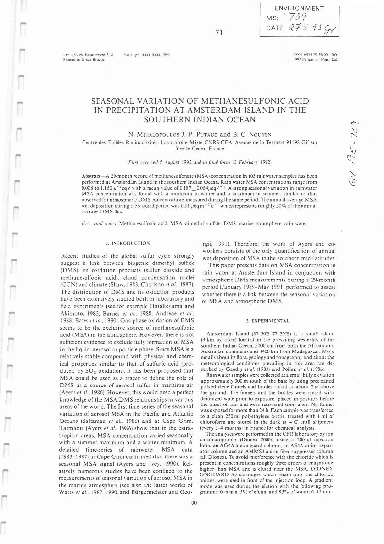
~f nt•"rii ,·r11· f.11nr1111n1t·nt \ ' 111 Pnn1c=d 1r: ürc;,11 Hn1:.11n.
. s ,, o. rr 1nll'1 ().)(lt) . 199 ;
71
ENVIRON MENT MS: ,· 73 o/ DATE: ·=<1 ·S- i 3 f-v'
00(\.I t,9XI 9: $t,(l0-0.()f l
199~ Per~am0r. Pre~:,, L td.
SEASONAL V ARIA TI ON OF METHANESULFONIC ACID IN PRECIPITATION AT AMSTERDAM ISLAND IN THE
SOUTHERN INDIAN OCEAN
N. MIHALOPOüLOS J .-P. PüTAlJD and B. C. NGUYEN
Centre des Faibles Radioactivités. Laboratoire Mixte CNRS-CEA. Avenue de la Terrasse 91198 Gif sur Yvette Cedex. France
!Firsr recein.'d 5 A11y11s1 1992 a11d in/inalfnrm 12 Fehruar_r 1992)
Abstract- A 29-month record of methanesulfonate (MSA) concentration in 103 rainwater samples has been performed at Amsterdam Island in the southern Indian Ocean. Rain water MSA concentrations range from 0.008 to 1.150 11 · 1 eq / with a mean ,·a lue of O. 187 ± 0.0541,eq 1- 1. A strong seasonal variation in rainwater MSA concentration was found with a minimum in winter and a maximum in summer. similar to that observed for atmospheric OMS concentrations measured during the same period. The annual average MSA wet deposition du ring the st udied period was 0.51 µeq m • 2 d- 1 which represents roughly 20% of the annual average OMS flux .
}-;_e_r ,rn,d index: Methanesulfonic acid. MSA. dimethyl sulfide. OMS. marine atmosphere. rain water.
1. l'.\TRODL'CTIO'.\
Recent studies of the global sulfur cycle strongly
suggest a link between biogenic dimethyl sulfide
(OMSI. its oxidation products (sulfur dioxide and
methanesulfonic acid). cloud condensation nuclei
(CCN) and climate (Shaw. l 983: Charlson et al .. 1987).
The distribution of OMS and its oxidation products
have been extensively studied both in laboratory and
field experiments (see for example Hatakeyama and
Akimoto. 1983: Barnes et al .. 1988: Andreae et al ..
l 988: Ba tes et al .. 1990). Gas-phase oxidation of OMS
seems to be the exclusive source of methanesulfonic
acid (MSA) in the atmosphere. However. there is not
sufficient evidence to exclude full y formation of MSA
in the liquid. aerosol or particle phase. Since MSA is a
relatively stable compound with physical and chem-
ical properties similar to that of sulfuric acid (pro-
duced by S02 oxidation). it has been proposed that
MSA could be used as a tracer to define the role of
OMS as a source of aerosol sulfur in maritime air
(Ayers et al., 1986). However. this would need a perfect
knowledge of the MSA.DMS relationships in various
areas of the world. The first time-series of the seasonal
variation of aerosol MSA in the P acifie and Atlantic
Oceans (Saltzman er al .. 1986) and at Cape Grim,
Tasmania (Ayers et al., 1986) show that in the extra-
tropical areas. MSA concentration varied seasonally
with a summer maximum and a winter minimum. A detailed time-series of rainwater MSA data ( 1983-1987) at Cape Grim confirmed that there was a
seasonal MSA signal (Ayers and Jvey. 1990). Rel-
atively numerous studies have been confined to the
measurements ofseasonal variation ofaerosol MSA in the marine atmosphere (see also the latter works of
Watts et al .. 1987. 1990. and Bürgermeister and Geo-
001
rgii. I 991 ). Therefore. the work of Ayers and co-
workers consists of the only quantification of an nuai
wet deposition of MSA in the southern mid-latitudes.
This paper presents data on MSA concentration in
rain water at Amsterdam Island in conjuction with
atmospheric OMS measurements during a ::!9-month
period (January 1989-May 1991) performed to assess
whether there is a link between the seasonal variation
of MSA and atmospheric OMS.
2. EXPERl!\-1E:":TAL
Amsterdam Island (37 50'S-77 ' 30'E) is a small island (9 km by 5 km) located in the prevailing westerlies of the southern lndian Ocean. 5000 km from both the African and Austrailan continents and 3400 km from Madagascar. More details about its flora. geology and topography and about the meteorological conditions prevailing in this area are de-scribed by Gaudry et al. ( 1983) and Polian el al. ( 1986).
Rain water samples were collected at a small hilly elevation approximately 300 m south of the base by using preclcaned polyethylene funnels and boilles raised at about 2 m above the ground. The funnels and the bottles were rinsed with deionized wate prior to exposure. placed in position beforc the onset of rain and were recovered soon aftcr. No funnel was exposed for more than 24 h. Each samplc was transferrcd to a clean 250 ml polyethylene boule. treated with I ml of chloroform and stored in the dark at 4·C until shipment (every 3--4 months) in France for chemical analysis.
The analyses were performed in the CFR laboratory by ion chromatography (Oionex 2000i) using a 200-µl injection loop. an AG4A anion guard column. an AS4A anion separ-ator column and an AMMSI anion fiber suppresser column (ail Oioncxl. To avoid interference with the chloride which is present in concentrations roughly threc orders of magnitude higher than MSA and is eluted near the MSA. O1O1\:EX ONG UAR O Ag cartridges which retain onh the chloridc anions. were us;d in fro~t of the injection lo~p. A gradient mode was used during the elullon with the following pro-gramme: 0-6 min. 5% of elu:rnt and 95°'o or water: 6-15 min.
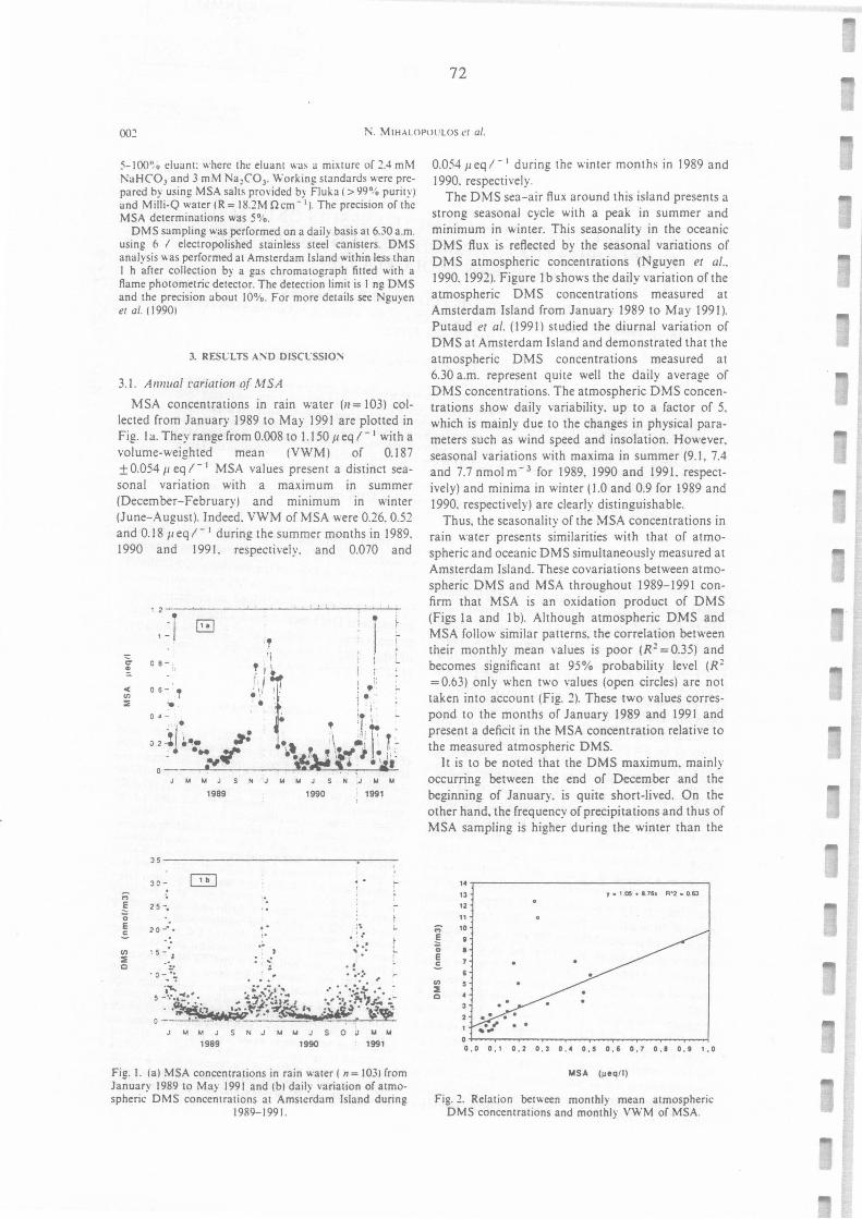
72
002 N. MIHALOPOl 1LOS t'/ al.
5-100'\o cluant: wherc the eluant was a mixture of 2.4 mM NaHCO3 and 3 mM Na 2CO 3• Working standards were prc-pared by using MSA salts pro\'ided by Fluka ( > 99% purity) and Milli-Q water(R= 18.2Mncm- 1 ). The precision of the MSA detcrminations was 5''/o.
DMS sampling was pcrformed on a daily basis at 6.30 a.m. using 6 / electropolished stainless steel canisters. DMS analysis was performed at Amsterdam Island within Jess than 1 h after collection by a gas chromatograph filled with a flame photometric detector. The detection limit is I ng DMS and the precision about 10%. For more details see Nguyen et al. ( 1990)
3. RESL"LTS A!\D DISCLSSIO:'\
3. 1. A111111al rariarion 1?( l\,fSA
MSA concentrations in rain water (11 = 103) col-lected from January 1989 to May 1991 are plotted in Fig. 1 a. They range from 0.008 to 1.150 JI eq 1- 1 with a volume-weighted mean (VWM) of 0.187 ± 0.054 JI eq r I MSA values present a distinct sea-sonal variation with a maximum in summer (December-February) and mmtmum in winter (June-August). lndeed. VWM of MSA were 0.26. 0.52 and 0.18 ;1 eq r I during the summer months in 1989. 1990 and 1991. respectively. and 0.070 and
.., ~ 0 E C
VI ::1: 0
0 8-:1
' ' 1
î î
r r:., 06~, Nj ._ 1 it _ 0 • - • . . • • :r \. -02.11~·- ~ !·, \ ..:: .. 1· r~
• •.. -~ li ' • .,,,, I • : · :,"' W.\ii .f • • i&•
JMMJ SNJM .MJ SN 1JMM
1989 1990 1991
35---------------,---JC- . -2 S -.
2 0 -- • :~
i.• 1 5 - ·, ' • •
:.• . ·. : . ,:
!.
f L
' , !) -.:; • ~. :- ,
.• "'L... •• •':' ,·.. •• •• • • .-:.; •• .. 5 -•: •• ~:1:. .,. !;•~';;;:. I •,,•:•, :-;.).,;; :.-
• -~ . ., ... -~f.~-:r~ h -~. -~ .. 0 ---·-· -~ .. ' •
JMMJSNJMMJSOJMM
1989 1990 1991
Fie. 1. (al MSA concentrations in rain water ( n = 103) from Ja~uarv 1989 to Ma,· 1991 and (b) dailv \'ariation of atmo-spheric· DMS conce~trations at Amste.rdam Island during
1989-1991.
0.054 ;1 eq 1- 1 du ring the winter months in 1989 and 1990. respectively .
The DMS sea-air flux around this island presents a strong seasonal cycle with a peak in summer and minimum in winter. This seasonality in the oceanic DMS flux is reflected by the seasonal variations of DMS atmospheric concentrations (Nguyen et al ..
1990. 1992). Figure I b shows the daily variation of the atmospheric DMS concentrations measured at Amsterdam lsland from January 1989 to May 1991). Putaud er al. ( 199 Il studied the diurnal variation of DMS at Amsterdam lsland and demonstrated that the atmospheric DMS concentrations measured at 6.30 a.m. represent quite well the daily average of DMS concentrations. The atmospheric DMS concen-trations show daily variability. up to a factor of 5. which is mainly due to the changes in physical para-meters such as wind speed and insolation. However. seasonal variations with maxima in summer (9.1. 7.4 and 7.7 nmol m - 3 for 1989, 1990 and 1991. respect-ively) and minima in winter (1.0 and 0.9 for 1989 and 1990. respectively) are clearly distinguishable.
Thus, the seasonality of the MSA concentrations in rain water presents similarities with that of atmo-spheric and oceanic DMS simultaneously measured at Amsterdam lsland. These covariations between atmo-spheric DMS and MSA throughout 1989-1991 con-firm that MSA is an oxidation product of DMS (Figs la and lb). Although atmospheric DMS and MSA follow similar patterns. the correlation between their monthly mean values is poor (R 1 = 0.35) and becomes significant at 95% probability level (R 1
=0.63) only when two values (open circles) are not taken into account (Fig. 2). These two values corres-pond to the months of January 1989 and 1991 and present a deficit in the MSA concentration relative to the measured atmospheric DMS.
lt is to be noted that the DMS maximum, mainly occurring between the end of December and the beginning of January. is quite short-lived. On the other hand. the frequency of precipitations and thus of MSA sampling is higher during the winter than the
1•
13 y • 1 0$ • 8 71h R~2 .. 0.63
12
11
;:;- 10
~ • 0 • E
=-Il)
::1: 0
0 +---~-~~-~~---..----.-----! o,o 0,1 0 , 2 o,3 o.• o,s o,, 0,1 0 , 1 o,t 1,0
MSA (µeq/1)
Fig. 2. Relation between monthly mean atmospheric DMS concentrations and monthly VWM of MSA.
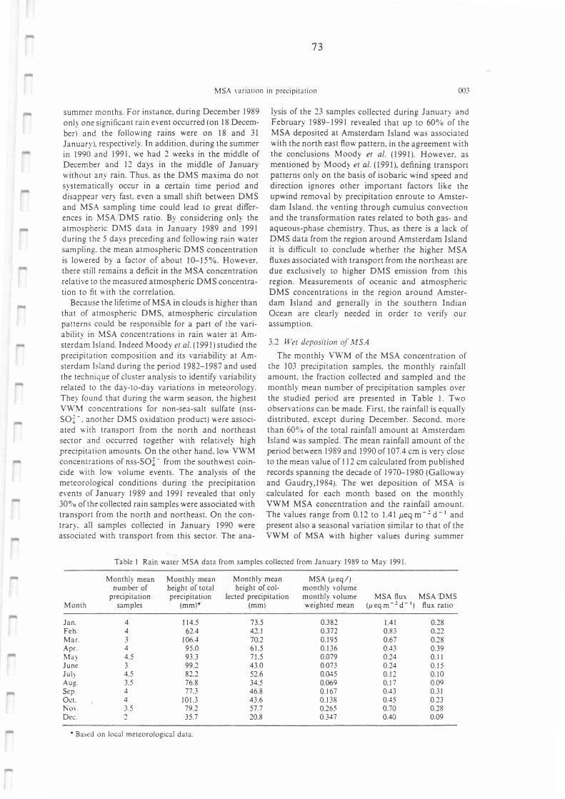
73
MSA variat io n in precipitati on 003
summer months. For instance. du ring December 1989 only one significant rain event occurred (on 18 Decem-ber) and the following rains were on 18 and 31 January). respectively . In addition. during the summer in I 990 and l 99 l. we had 2 weeks in the middle of December and 12 days in the middle of January without any rain. Thus, as the DMS maxima do not systematically occur in a certain time period and disappear very fast. even a small shift between DMS and MSA sampling time could lead to great differ-ences in MSA/ DMS ratio. By considering only the atmospheric DMS data in January 1989 and 1991 during the 5 days preceding and following rain water sampling. the mean atmospheric DMS concentration is lowered by a factor of about 1~15 %. However. there sti ll remains a deficit in the M SA concentration relati ve to the measured atmospheric DMS concentra-tion to fit with the correlation.
Because the Iifetime ofMSA in clouds is higher than that of atmospheric DMS, atmospheric circulation patterns could be responsible for a part of the vari -ability in MSA concentrations in rain water at Am-sterdam Island. lndeed Moody et al. ( 1991) studied the precipitation composition and its variability at Am-sterdam Island during the period 1982- 1987 and used the technique of cluster analysis to identify variability related to the day-to-day variations in meteorology. They found that during the warm season. the highest VWM concentrations for non-sea-salt sulfate (nss-SOi -. another DMS oxida·tion product) were associ-ated with transpo rt from the north and northeast sector and occurred together with relatively high precipitation amounts. On the other hand. low VWM
concentrations of nss-SOi- from the southwest coïn-cide with low volume events. The analysis of the meteorological conditions during the precipitation e,·ents of January 1989 and l 991 revealed that onl y 30°10 of the collected rain samples were associated with transport from the north and northeast. On the con-trary. ail samples collected in January 1990 were associated with transport from this sector. The ana-
lysis of the 23 samples collected during January and February 1989-1991 revealed that up to 60% of the MSA deposited at Amsterdam Island was associated with the north east flow pattern. in the agreement with the conclusions Moody et al. (1991). However. as mentioned by Moody et al. (1991 ). defining transport patterns only on the basis of isobaric wind speed and direction ignores other important factors Iike the upwind removal by precipitation enroute to Amster-dam Island. the venting through cumulus convection and the transformation rates related to both gas- and aqueous-phase chemistry. Thus. as there is a Jack of DMS data from the region around Amsterdam Island it is difficult to conclude whether the higher MSA fluxes associated with transport from the northeast are due exclusively to higher DMS emission from this region. Measurements of oceanic and atmospheric DMS concentrations in the region around Amster-dam Island and generally in the sou thern lndian Ocean are clearly needed in order to verify our assumption.
3.2 Wer deposirion of MSA
The monthly V\VM of the MSA concentration of the 103 precipitation samples. the monthly rainfall amount. the fraction collected and sampled and the monthly mean number of precipitation samples over the studied period are presented in Table l. Two observations can be made. First. the rainfall is equally distributed, e:~cept during December. Second. more than 60% of the total rainfall amount at Amsterdam Island was sampled. The mean rainfall amount of the period between 1989 and 1990 of 107.4 cm is very close to the mean value of 112 cm calculated from published records spanning the decade of 197~ 1980 (Galloway and Gaudry,I 984). The wet deposition of MSA is calculated for each month based on the monthly VWM MSA concentration and the rainfall amount. The values range from O. 12 to 1.41 µeq m - 1 d - 1 and present also a seasonal variation similar to that of the VWM of MSA with higher values during summer
Table I Rain water MSA data from sa mplcs collected from January 1989 to May 1991.
Monthly mean Monthly mean Monthly mean MSA (/leqf) number of height of total heigh t of col- monthly rnlume
precipitation precipitation kcted precipitation monthly volume MSA flux MSA 'DMS Mont h samples (mm)* (mm) weighted mean (µ eq m - 1 d - 1 ) flux ratio
Jan. 4 114.5 73.5 0.382 1.41 0.28 Feb. 4 62.4 42.1 0.372 0.83 0.21
Mar. 3 106.4 70.2 0.195 0.67 0.28 Apr. 4 95.0 61.5 0.136 0.43 0.39 May 4.5 93.3 71.5 0.079 0.24 0. 11 June 3 99 .2 43.0 0.073 0.24 0.15 July 4.5 82.2 52.6 0.045 0.12 0.10 Aug. 3.5 76.8 34.5 0.069 0.1 7 0.09 Sep. 4 77.3 46.8 0.167 0.43 0.31 Oct. 4 101.3 43.6 0. 138 0.45 0.23
N o v. 3.5 79.2 57.7 0.265 0.70 0.28 Dec. 2 35.7 20.8 0.347 0.40 0.09
• Based on local metcorological data .
74
N. M!HALO POL' LOS l'I a/.
months and minimum during winter. During the studied period. the mean wet deposition of MSA was 0.51 Jteq m - 2 d - 1 which is a factor of 2 higher than that measured at Cape Grim. using a similar method for MSA determination in rain water (0.26
1ieq m - 2 d - 1: Ayers et al.. 1991 ). This factor results
from both higher mean rainfall amount (about 50¾) and from higher mean VWM of MSA at Amsterdam Island (0.187 ± 0.05411 eq r- 1
: this work: measure-ments from 1989 to 1991) than at Cape Grim (0.12 ± 0.03peq r- 1
: measurements from 1983 to 1987: Ayers and Ivey 1990). It is to be noted that from 1990 to 1991. the mean atmospheric DMS concentrations at Amsterdam Island (Nguyen et al. , 1992. this work) were 30-40¾ greater than those of Cape Grim (Ayers ec al.. 1991 ). These differences cou Id reflect the spatial and temporal variability of the DMS fluxes .
From the seawater DMS concentration at Amster-dam Island. the windspeed-dependent exchange coef-ficient iK,..) and a gas exchange mode] (Liss and Merlivat. 1986). Nguyen et al. (1990. 1992). have calculated an annual average DMS flux of 2.2 11 mol m - 1 d - 1 for the 1989-90 period. lt should be noted that the exchange coefficient (Kwl is highly uncertain and that different approaches in calculating J.:.~ can lead to differences as large as a factor 1.8 (Erickson et al .. 1990). The DMS flux is therefore calculated with an uncertainty of a factor at least 2. The annual average wet deposition of MSA of 0.51 11 mol m 2 d- 1 calculated here is about 20¾ the an nuai average DMS flùx. lt is worthwhile noting that we have to be very · careful when we examine the MSA 'DMS ratio as the frequency of the sampling is not the same. DMS in sea water was measured roughly every 3 days and MSA in rain water was collected four times a month. This could be crucial during summer when DMS presents its highest vari-ability and can explain the lowest ratio observed during December when the fewest rainwater samples were collected.
Table 1 shows the variability of the ratio of the monthly MSA wet deposition versus the oceanic DMS flux. The MSA/ DMS ratio was significantly lower during winter months despite the scatter in the data. This observation agrees well with the conclusions of Putaud et al. (1992). These authors, by using a photo-chemical box mode! and the simultaneously measured atmospheric concentrations of S0 1 and DMS at Amsterdam Island during the 1989-90 period, have found that about 70¾ of the DMS is oxidized to SO2 ,
the remaining part is transformed in MSA, DMSO and DMSO1. In addition. Putaud et al. (1992) have found that the best fit between the measured and computed SO2 concentrations was obtained assuming a seasonal dependence in the branching ratio of DMS oxidation with higher MSA yield in spring and sum-mer (up to 0.3-0.4) and lower in wint_er (up to 0.1) in agreement with our observations. Note also that Ayers et al. (1991) have observed the same seasonal
pattern in the MSA-'nss-SOi - concentration at Cape Grim.
However. it is difficult to ex plain the reasons of the seasonality in the MSk DMS flux ratio as it is con-trary to the explanation most commonly advanced . Indeed. from laboratory experiments Hynes et al.
( 1986) have found a negative temperature dependence in the ratio of the two pathways (abstraction/addition) of the DMS oxidation by OH radicals. Based on the observations of Hynes et al. ( 1986). Berresheim ( 1987) assumed that the addition and the abstraction path-ways lead exclusively to the formation of MSA and S0 1, respectively, and suggested that the lower tem-peratures favor MSA production. Following Berresheim"s calculations. we expect a MSA/DMS ratio of 40¾ and 32% during the cold and warm seasons. respectively, which is contrary to our obser-vations as well with th ose of Ayers et al. ( 1991 ). However. up to now there is no indication from laboratory experiments to support that the addition and the abstraction pathways lead exclusively to the formation of MSA and SO 2, respectively. The most recent work (Yin et al. 1990) has shown that MSA can result from both channels. More information about the factors controlling the MSA production from DMS oxidation are clearly needed to explain the seasonality in the MSA.1DMS flux ratio.
4. co-..CLIJSIO~
MSA concentrations have been determined in rain-water samples (11 = 103) at Amsterdam Island from January 1989 to May 1991. A very strong seasonal variation in rain water MSA concentration and wet deposition is found with a summer maximum and a winter minimum. thus presenting close similarities to that observed for atmospheric DMS concentrations measured at the same point during the same period. The 29 months of rainwater MSA data show an annual average wet deposition rate of 0.51 µeq m - 2 d - 1
, which accounts for about 20% of the annual average oceanic DMS flux calculated for this area. This figure has to be viewed with a lot of caution as an absolute value, since the frequency of the DMS and MSA samplings was not the same and since the DMS flux is given with an uncertainty of a factor of 2. However, it is worthwhile noting that in relative terms the MSA/DMS ratio presents a seasonality with higher values in summer probably rcflecting a higher yield of MSA from DMS oxidation during summer. Additional information about the factors controlling the MSA production from DMS oxidation as well as concurrent measurements of size-distributed aerosol of MSA, MSA in rain water. DMS and SO 2 over an extended time period would certainly be very inter-esting and rewarding. and may go towards solving some of the uncertainties m the seasonality of the MSA .. DMS flux ratio.
-
75
MSA variation in precipit ati on 005
Ac/..11 /lld,•dµt'111t•111 .,-- Wc thank P. Lahoz and L. Gallet for MSA measurement s. J. C. Duples~y. G . Lambert. M . Kanak i-do u. A. M cTaggart and an unkno wn revicwer for helpful comments. This work was supported by the Territoire des Terres Australes et Antarctiques Françaises. the Centre Nat ional de la Recherche Scientifique and Commissariat à l"Energic Atomique. This is CFR contribution No. 1353.
REFERE:\CES
Andreac M . O .. Berresheim H .. Andreae T. W .. Kritz M . A .. Ba tes T. S. and Merrill J. T. ( 1988) Vertica l distribution of dimethylsulfide. sulfur dioxide. aerosol ions and radon a,·er the no rtheast Pacifie ocean. J . armos. Chem . 6. 149- 173.
Aye rs G . P .. lvey J. P. ( 19901 Methanesulfona te in rainwater at Cape Grim. Tasmania Tel/us 40B. 297-307.
Ayers G . P .. lvey J. P. and G oodman H. S. ( 1986) Sulfate and methanesulfonate in the ma ritime aerosol at cape Grim. Tasmania J. armas. Chem. 4. 173- 185.
Ayers G . P .. lvey J . P. and Gillett R. W. (1991) Coherence between seasonal cycles of dimethvl sulfide. methanesul-phonate and sulphate in marine ai(. !Varure 349. 404-406.
Barnes 1.. Bastian V .. and Becker K . H. ( 1988) Kinectics and mechanisms of the reactio n of OH rad icals with dimethvl sulfide. lnr. J. Chem. /ù11er. 20. 415-431. ·
Ba tes T. S .. Johnson J. E .. Quinn P. K .. G o ldan P. D . Kuster W . C.. Co,ert D . C. and Hahn C. J. (1990) The bio-geochemical sulfur cycle in the marine boundarv laver over the m; rtheast Pacifie Ocea n. J . armos . Chem. io. 59-81.
Berresheim H. ( 1987) Biogenic sulphur emission fro m the Suba ntarctic and Antarctic Oceans. J . geophys. Res. 92. i 3~45-1 3262.
Bürgermeister S. and Georgii H.-W. ( 19911 Distribution of methanesulfona te. nss sulfate and dimethvlsulfide over the Atla ntic and the N o rth Sea. A1mospheri<: Eni-ironmem 25. 587-595.
Charlson R. J .. Lovelock J. E .. Andreae M . O . and Warren S. G. (1987) Oceanic phytoplankton atmospheric sulphur. cloud albedo and climate: a geophysiological feedback . .\' awre 326. 655-661.
Erickson D . J .. Ghan S. J .. Penner J. E. ( 19901 Global ocean to atmosphere dimethylsulfide flux. J . geophys. Res. 95. 7543- 7552.
Galloway J. N. and Gaudr:-, A. (1984) The composition of precipitation of Amsterdam Island. lndian Ocean. A1mo-
spheric Enriro11men1 18. 2649-2656. Gaudry A .. Ascencio J . M . and Lambert G (1983) Pre-
liminary studv of CO , variations at Amsterdam Island (Terres Austr~les et A~tarctiques Francaises). J . geaphys.
Re~. 88, 1323- 1329. Gau rd y A .. A. Polian G .. Ardouin B. and Lambert. G . ( 1990).
Radon-ca libratcd emissions of CO , from South Africa. Tel/us 42B. 11 - 21. •
Hatakeyama S. and Akimoto H . (1983) Reactions of OH radicals with me thanethiol. dimcthvlsulfide and dime thvl disulfide in air. J. phys. Chem. 87. 2387-2395. ·
Hynes A. J .. Wine P. H .. Semmes D. H. ( 1986) Kinct ics and mechanisms of OH reactions with organic sulfides J. phys. Chem 90, 4148--4156.
Liss. P. S. and Merlivat L. (1986) The Role of Air-Sea
Excha11ge in Geochemical Cycling (edited by Buat-Ménard P .. pp. I l3- l 27D. Reidel Dordrecht.
Moody J. L.. Psyenny A. P. P .. Gaudrv A .. Keene W. C.. Galloway J. N. and Polian G .. (1991).Precipitation com-position and its variability in the southern lndian Ocean: Amsterdam island. 1980-1987. J. geophys. Res. 96.
20769-20786. Nguyen B. C.. Mihalopoulos N. and Belviso S. ( 1990) Sea-
sonal variation of atmospheric dimethylsulfide at Amster-dam island in the southern lndian Ocean. J. aimas. Chem.
Il , I 23-143. Nguyen B. C.. Mihalopoulos N ., Putaud J. P .. Gaudrv A ..
Gallet L.. Keene W.C. and Galloway J . N . (1992) Co~·ari-ations of oceanic dimethysulfide. its oxidation products and rain acidity at Amsterdam island in the southern lndian Ocean. J. armas. Cltem. 15, 39-53.
Polian G .. Lambert G .. Ardouin B. Jégou A. (1986) Long range transport of continental radon in subantarctic areas. Tel/us 38B, 178- I 89.
Putaud J. P .. Mihalopoulos N. Nguyen B. C.. Campin J. M. and Belviso S. ( 1991) Seasonal variations of atmospheric sulfur dioxide and dimethylsulfide concentrations at Amsterdam island in the Southern lndian Ocean. J . aimas.
Chem. Il, 117-131. Saltzman E. S .. Savoie D. L.. Zika R. G . and Prospero J. M .
( 1983) l'vlethanesulfonic acid in the marine atmosphere. J. geaph_i-s. Res. 88. 10897-1090.2.
Saltzman E. S .. Savoie D . L.. Prospero J. M. and Zika R. G . ( 1986) Methanesulfonic acid and non-sea-salt sulfate in Pacifie air: regional and seasonal variations J. a1mos.
Cltem. 4, .227-240. Shaw ( 19831 Bio-controlled thermostasis involvine the sulfur
cycle. Clim. Change 5. 297-303. -Watts S. F .. Watson A. and Brimblecomble P. ( 1987) Meas-
urements of the aerosol concentrations of methanesulfonic acid. dimethylsulphoxide. and dimethylsulphone in the marine atmosphere of the British Isles. Armospheric Enrir-
onmen1 21, 2667-2672. Watts S. F., Brimblecomble P. and Watson A. (1990). Meth-
anesulphonic acid. dimethylsulfoxide and dimethyl sui-phone in aerosols. A1mospheric Endranmenr 24, 353-359.
Yin F .. Grosjean D. and Seinfeld J . H. ( 1990) Photooxidation of dimethvlsulfide and dimethvldisulfide. 1. Mechanism developm~nt. J. acmos. Chem. Ù, 309-399.

L
77
Il. C. IMPACT DES PRODUITS D'OXYDATION DU SULFURE DE DIMETHYLE SUR L'ACIDITE
NATURELLE DES PRECIPITATIONS.
L'influence des composés soufrés anthropogéniques sur l'acidité des précipitations dans
les régions industrialisées est aujourd'hui bien établie. Mais quelle est la cause de leur
acidité dans les régions non polluées, et particulièrement marines, où le lessivage des
embruns devrait conduire à une augmentation du pH de l'eau de pluie ? En premier lieu, une
fraction de l'acidité provient de l'équlibre entre le C02 atmosphérique et le C02 dissous dans
les gouttelettes(! l, qui amènerait le pH d'une eau de pluie "pure" à une valeur proche de 6,
fonction de la température. Mais le pH des précipitations mesuré à Amsterdam est en
moyenne plus bas encore.
Dans l'article suvant, nous présentons les covariations entre les concentrations de
composés soufrés et l'acidité de l'eau de pluie observées à l'île Amsterdam. Les rapports de
ces concentrations dans l'eau de pluie permettent d'évaluer la contribution des produits
d'oxydation du DMS à l'acidité en excès(2hdes précipitations.
1 La dissolution de C02 dans l'eau conduit aux équilibres suivants:
C02(atmosph.) <=> C02(dissous) C02(d) + H20 <=> H+ + HC03-
HC03- <=> H+ + coi-Dans la gamme de pH habituelle de l'eau de pluie des régions océaniques, l'espèce HC03- est majoritaire.
2 Nous avons défini l'acidité en excès (AEX) comme:
AEX = [H+Jmesuré - [H+Jc02 [H+Jco2 étant la concentration d'ions H+ découlant des équilibres décrits ci-dessus, calculée à partir de la
concentration atmosphérique du C02 et de la température.

t
,...
79
.!011rnal of A/!nospheric Che111is1ry 15: 39-53. 1992. © 1992 K lwver Arndemic l'ubfühers. l'ri111ed in 1he Ne1herlands.
Covariations in Oceanic Dimethyl Sulfide,
its Oxidation Products and Rain Acidity at
Amsterdam Island in the Southern Indian Ocean
B. C. NGUYEN. N. MIHALOPOULOS. J. P. PUTAUD. A. GAUDRY. L. GALLET Ce111re des Faibles Radioac1i1ùés. Labora1oire i'Vlixœ C.\'RS-C'EA. .-\1·e11ue de la Terrasse 91198, Cifs11r-Y1·eue. Cedex. France
W.C. KEENE and J. N. GALLOWAY Enviro11me111al Sciences Depar1me111. U11i1·ersiiy of Virginia. Clwrlouesville. Virginia. 22903 U.S.A.
(Received: 25 June 1991)
39
Abstract. Simultaneous measurements of rain acidity and dimethyl sultïde (OMS) at the ocean surface and in the atmosphere were performed at Amsterdam Island over a -+ year period. During the last 2 years. measuremen ts of sulfur dioxide (SO, ) in the atmosphere and of methane sulfonic acid (MSA) and non-sea-salt-sulfate (nss-SO_i- ) in rainwater were also performed. Covariations are observed between the oceanic and atmospheric OMS concentrations. atmospheric SO, concentrations. wet c.leposition of MSA. nss-SO_i-. and rain acidity. A comparable summer to winter ratio of OMS and SO, in the atmosphere and MSA in precipitation were also observed. From the chemical composition of rrecipitation we estimate that OMS oxidation products contribute approximately 40% of the rain acidity. If we consider the acic.lity in excess. then OMS oxidation products contribute about 55%.
Key words. Oceanic dimethyl sulfide. atmospheric dimethyl sulfide. sulfur dioxide. wet deposition. 11011-sea-salt sulfate. methanesulfonic acid. rain acidity.
1. Introduction
Biological activity of phytoplankton and zooplankton in surface seawater releases about 15 to 40 Tg S/ yr ( 1 Tg= 10 12 g) of dimethyl sulfide (OMS) into the atmos-phere (Lovelock e, al .. 1972; Nguyen et al .. 1978, 1983; Andreae and Raemdock. 1983; Andreae. 1986; Bates et al., 1987a). This gas rapidly oxidizes in the atmos-phere to give methane sulfonic acid (MSA) and sulfur dioxide (SO2) which subse-quently reacts to form H 2S0; (Bonsang et al., 1980; Saltzman et al., 1983; Nguyen et al., 1983; Ayers et al .. 1986; Pszenny et al., 1989). These aerosols (MSA and H 2S0; ) can act as cloud condensation nuclei (CCN), influencing albedo and. therefore, the Earth's climate (Shaw. 1983; Nguyen et al .. 1983; Charlson et al..
1987; Bates et al .. 1987b). Moreover. MSA and H,SO; can also contribute to the natural acidification of rain water.
Due to its importance in atmospheric chemistry. considerable effort has been made in the last few years to better understand the seasonal variation in OMS and
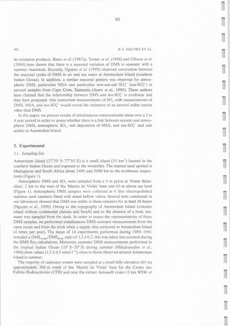
80
40 B. C. NGUYEN ET AL
its oxidation products. Bates et al. (1987a), Turner et al. (1988) and Gibson et al.
( l 990) have shown that there is a seasonal variation of OMS in seawater with a summer maximum. Recently, Nguyen et al. (l 990) observed covariation between the seasonal cycles of OMS in air and sea water at Amsterdam Island (southern Indian Ocean). In addition, a similar seasonal pattern was observed for atmos-pheric OMS, particulate MSA and particulate non-sea-salt SOt (nss-SOt) in aerosol samples from Cape Grim, Tasmania (Ayers et al., 1990). These authors have claimed that the relationship between OMS and nss-SOt is nonlinear and they have proposed that concurrent measurements of S0 2 with measurements of OMS. MSA, and nss-SOt would reveal the existence of an aerosol sulfur source other than OMS.
In this paper, we present results of simultaneous measurements taken over a 2 to 4 year period in order to assess whether there is a link between oceanic and atmos-pheric OMS, atmospheric S0 2, wet deposition of MSA. and nss-SOt and rain acidity at Amsterdam Island.
2. Experimental
2.l. Sampling Site
Amsterdam Island (37°50' S-77°30' E) is a small island (55 km 2) located in the
southern Indian Ocean and exposed to the westerlies. The nearest land upwind is Madagascar and South Africa about 3400 and 5000 km to the northwest. respec-tively (Figure l ).
Atmospheric OMS and S0 2 were sampled from a 9 m pylon at ·Pointe Béné-dicte·. 2 km to the west of the ·Martin de Viviès· base and 65 m above sea level (Figure 1 ). Atmospheric OMS samples were collected in 6 liter electropolished stainless steel canisters fitted with metal bellow valves. Severa! tests conducted in our Iaboratory showed that OMS was stable in these canisters for at least 36 hours (Nguyen et al., 1990). Owing to the topography of Amsterdam Island (volcanic island without continental plateau and beach) and to the absence of a boat. sea-water was sampled from the dock. In order to assess the representativity of these OMS samples, we performed simultaneous OMS seawater measurements from the open ocean and from the dock when a supply ship anchored at Amsterdam Island ( 4 times per year). The mean of 14 experiments performed during 1989-1991 revealed a OMS 0 ccan/OMSuock ratio of l.3 ± 0.2, this was taken into account during the OMS flux calculations. Moreover. seawater OMS measurements performed in the tropical Indian Ocean ( 10° S-20° S) during summer (Mihalopoulos et al ..
1988) show values ( l.5 ± 0.5 nmol 1- 1 ). close to those observed around Amsterdam
[sland in summer. The majority of rainwater events were sampled at a small hilly elevation (60 m)
approximately 300 m south of the ·Martin de Viviès' base for the Centre des Faibles Radioactivités (CFR) and near the extinct Antonelli crater (3 km WSW of
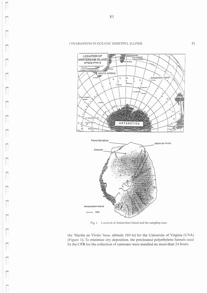
81
COVARIAT!ONS IN OCEAN!C D!METHYL SULF!DE
LOCATION OF AMSTERDAM ISLAND
37"50'S· 77":l1 'E
Antonelli
Amsterdam Island
- 1km
Manin de Viviès
Fig. 1. Location of Amsterdam Island and the sampling sites.
41
the ·Martin de Viviès' base. altitude 160 m) for the University of Virginia (UVA) ( Figure 1 ). To minimize dry deposition. the precleaned polyethylene funnels used by the CFR for the collection of rainwater were installed no more than 24 hours
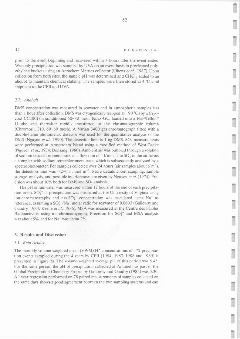
82
42 B. C. NGUYEN ET AL
prior to the event beginning and recovered within 4 hours after the event ended. Wet-only precipitation was sampled by UVA on an event basis in precleaned poly-ethylene buckets using an Aerochem Metrics collector (Likens et al., 1987). Upon collection from both sites, the sample pH was determined and CHCI 3 added to an aliquot to maintain chemical stability. The samples were then stored at 4 ·c until shipment to the CFR and UVA.
2.2. Analysis
OMS concentration was measured in seawater and in atmospheric samples Jess than I hour after collection. OMS was cryogenically trapped at -90 ·c (by a Cryo-cool CClO0) on conditioned 60-80 mesh Tenax-GC, Ioaded into a FEP-Teflon~ U-tube and thereafter rapidly transferred to the chromatographie column (Chromosil. 310. 60-80 mesh). A Varian 3400 gas chromatograph fitted with a double-flame photometric detector was used for the quantitative analysis of the OMS (Nguyen et al .. 1990). The detection limit is 1 ng OMS. S0 2 measurements were performed at Amsterdam Island using a modified method of West-Gaeke (Nguyen et al., 1974; Bonsang, 1980). Ambient air was bubbled through a solution of sodium tetrachloromercurate. at a flow rate of 4 1/min. The SO, in the air forms a complex with sodium tetrachloromercurate, which is subsequently analysed by a spectrophotometer. For samples collected over 24 hours (air samples about 6 m 3),
the detection limit was 0.2-0.3 nmol m--1_ More details about sampling. sample storage, analysis. and possible interferences are given by Nguyen et al. ( 1974 ). Pre-cision was about 10% both for OMS and S02 analysis.
The pH of rainwater was measured within 12 hours of the end of each precipita-tion event. sot in precipitation was measured at the University of Virginia using ion-chromatography and nss-SOt concentration was calculated using Na+ as reference. assuming a sot /Na+ molar ratio for seawater of 0.0603 (Galloway and Gaudry. 1984: Keene et al., 1986). MSA was measured at the Centre des Faibles Radioactivités using ion-chromatography. Precision for sot and MSA analysis was about 5%. and for Na+ was about 2%.
3. Results and Discussion
3.1. Rain Acidity
The monthly volume weighted mean (VWM) H+ concentrations of 172 precipita-tion events sampled during the 4 years by CFR ( 1984, 1987, 1988 and 1989) is presented in Figure 2a. The volume weighted average pH of this period was 5.45. For the same period, the pH of precipitation collected at Antonelli as part of the Global P_recipitation Chemistry Project by Galloway and Gaudry ( 1984) was 5.30. A linear regression performed on 78 paired measurements of samples collected on the same days shows a good agreement between the two sampling systems and can
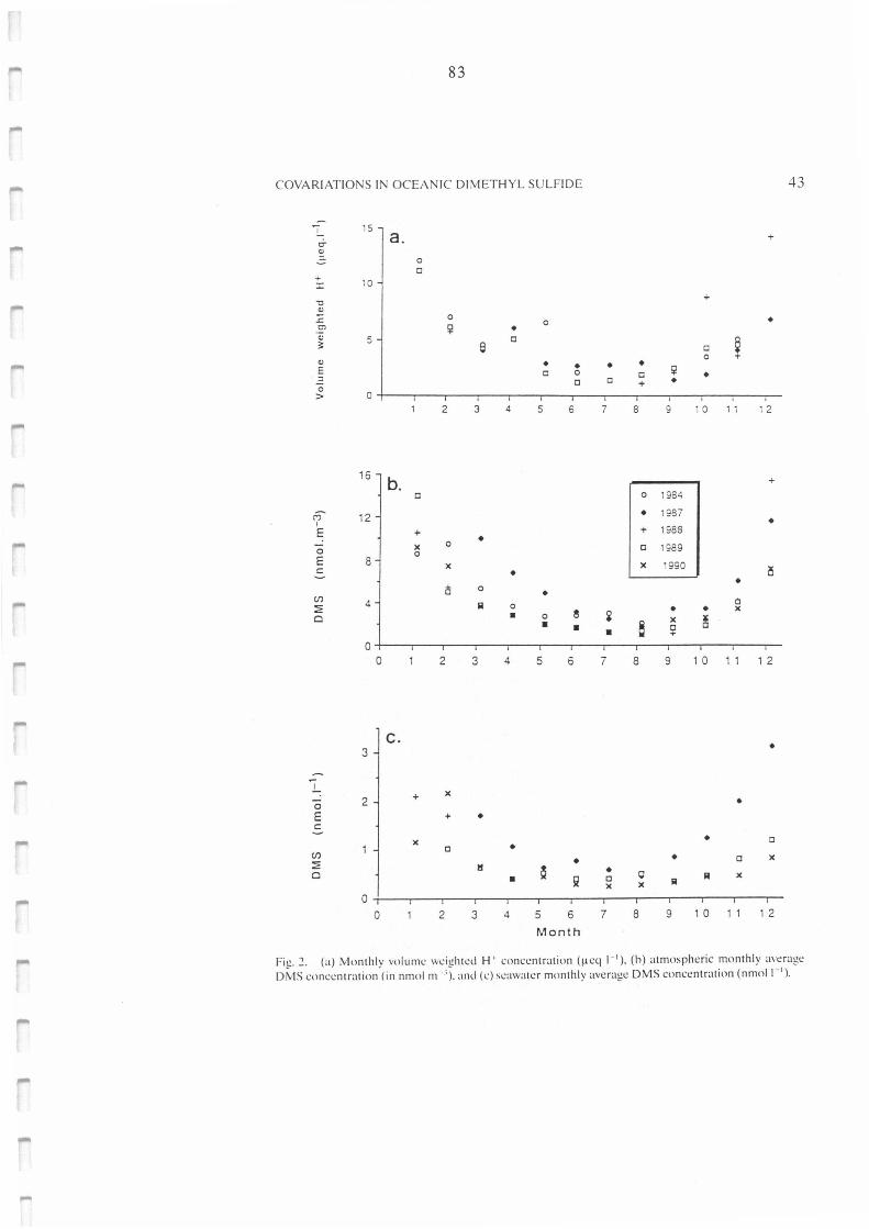
....
83
COYARIATIONS IN OCEANIC DIMETHYL SULFIDE 43
-!.... 15
& a. +
"' 0
C + 10 J:
+ "O
"' .c 0 • Ol !i!
0 • " 5 C
~ 3: e C
"' 0
E • • • • ::,
C 0 C !i! • C C + • 0 > 0
2 3 4 5 6 7 8 9 1 0 11 1 2
16 b. +
C 0 1984
€ 12 • 1987 1 • E + + 1988 ~ 0 • 0 X C 1989
0 E 8 X X 1990
-=- • 15 • i5 0 • (/l
4 0 ~ A 0
e • • X
0 • 0 i ~ X • • a ~ • 0
0 2 3 4 5 6 7 8 9 1 0 11 1 2
c. 3 •
.!.... X + 0 2 • E + • -=- X • C
C • (/l • X ~ • C
0 Il
~ • • 1( C 0 A X X X A
0 0 2 3 4 5 6 7 8 9 1 0 11 1 2
Month
Fig. 2. (a) Monthly vo lumc wcighteJ H ' cnnœntratinn (µc4 1- 1 ) . (b) atmospheric monthly a,eragc
DMS cnnœntration (in nmol m '). and (c) scawa1er mnnthly average OMS concentration (nmol 1- 1) •
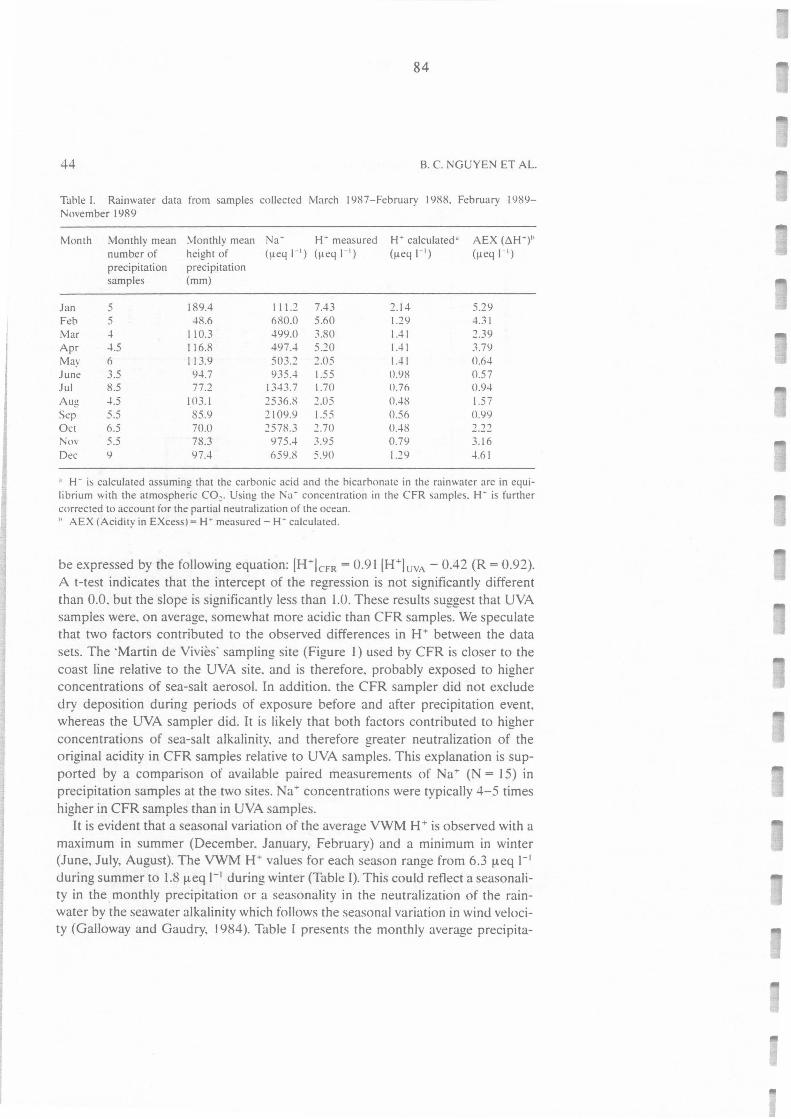
84
44 B. C. NGUYEN ET AL.
Tahle !. Rainwater data from samples collected March 1987-February 1988. February 1989-November 1989
Month Monthly mean \fonthly mean Na- H- measured H- calculated·' AEX(6W)" number of height of (µeq 1- 1) (rleq 1- 1
) (µeq 1- 1) (µeq 1- 1)
precipitation precipitation samples (mm)
Jan 5 189.4 111.2 7.43 2.14 5.29 Feb 5 -l8.6 680.0 5.60 1.29 -l.31 Mar -l 110.3 499.0 3.80 1.41 2.39 Apr -l.5 116.8 497.-l 5.20 1.-ll 3.79 May 6 113.9 503.2 2.05 Ut 0.6-l June 3.5 9-l.7 935.-l 1.55 0.98 0.57 Jul 8.5 77.2 1343.7 l.70 0.76 0.94 Aug -l.5 103.l 2536.8 2.05 (U8 1.57 Sep 5.5 85.9 2109.9 1.55 0.56 0.99 Oct 6.5 70.ü ~578.3 2.70 0.-l8 2.22 Nov 5.5 78.3 975.4 3.95 0.79 3.16 Üt!C 9 97.4 659.8 5.90 1.29 -l.61
·' H- is calculated assuming that the carbonic acid and the bicarbonate in the rainwater are in equi-librium with the atmospheric CO~. Using the Na- concentration in the CFR samplt!s. H- is further corrected to account for the partial neutralization of the ocean. " AEX (Acidity in EXœss) = H· measured - H- calculated.
be expressed by the following equation: [H+lcrn = 0.91 [H+luvA - 0.42 (R = 0.92). A t-test indicates that the intercept of the regression is not significantly different than 0.0. but the slope is significantly Jess than J.O. These results suggest that UVA samples were. on average, somewhat more acidic than CFR samples. We speculate that two factors contributed to the observed differences in H+ between the data sets. The ·Martin de Viviès' sampling site (Figure 1) used by CFR is closer to the coast line relative to the UVA site. and is therefore. probably exposed to higher concentrations of sea-salt aerosol. In addition. the CFR sampler did not exclude dry deposition during periods of exposure before and after precipitation event, whereas the UVA sampler did. It is likely that both factors contributed to higher concentrations of sea-salt alkalinity. and therefore greater neutralization of the original acidity in CFR samples relative to UVA samples. This explanation is sup-ported by a comparison of available paired measurements of Na+ (N = 15) in precipitation samples at the two sites. Na+ concentrations were typically 4-5 times higher in CFR samples than in UVA samples.
It is evident that a seasonal variation of the average VWM H+ is observed with a maximum in summer (December. January, February) and a minimum in winter (June, July, August). The VWM H+ values for each season range from 6.3 µeq 1- 1
during summer to l.8 µeq 1- 1 during winter (Table I). This could retlect a seasonali-ty in the . monthly precipitation or a seasonality in the neutralization of the rain-water by the seawater alkalinity which follows the seasonal variation in wind veloci-ty (Galloway and Gaudry. 1984 ). Table I presents the monthly average precipita-
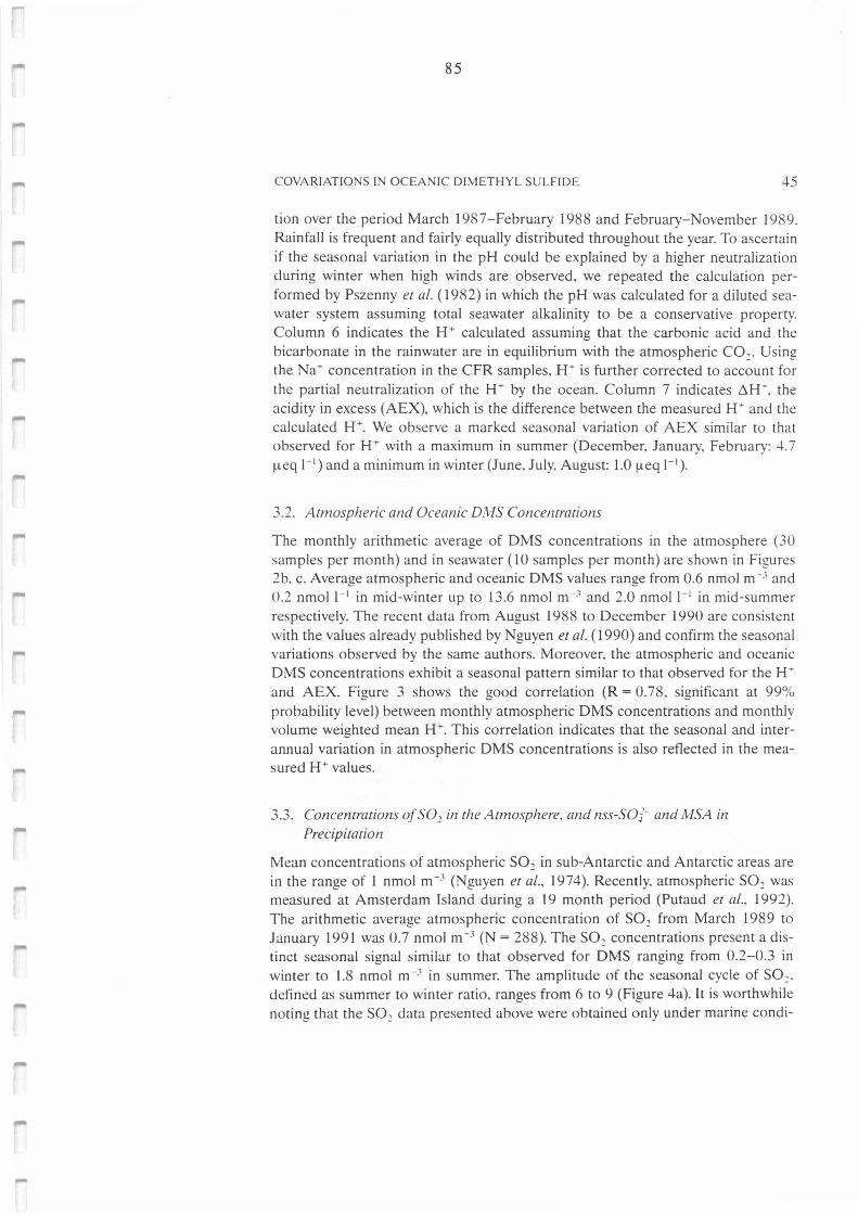
85
COYARIATIONS IN OCEANIC DIMETHYL SULFIDE 45
tian over the period March 1987-February 1988 and February-November 1989. Rainfall is frequent and fairly equally distributed throughout the year. To ascertain if the seasonal variation in the pH could be explained by a higher neutralization during winter when high winds are observed, we repeated the calculation per-formed by Pszenny et al. ( 1982) in which the pH was calculated for a diluted sea-water system assuming total seawater alkalinity to be a conservative property. Column 6 indicates the H + calculated assuming that the carbonic acid and the bicarbonate in the rainwater are in equilibrium with the atmospheric C0 2 . Using the Na+ concentration in the CFR samples, H+ is further corrected to account for the partial neutralization of the H+ by the ocean. Column 7 indicates ~H +, the acidity in excess (AEX). which is the difference between the measured H + and the calculated H +. We observe a marked seasonal variation of AEX similar to that observed for H + with a maximum in summer (Oecember, January, February: 4.7 µeq 1- 1) and a minimum in winter (June, July, August: 1.0 µeq 1- 1 ) .
3.2. Atmospheric and Oceanic DAIS Concentrations
The monthly arithmetic average of OMS concentrations in the atmosphere (30 samples per month) and in seawater (JO samples per month) are shown in Figures 2b. c. Average atmospheric and oceanic OMS values range from 0.6 nmol m-.1 and 0.2 nmol 1- 1 in mid-winter up to 13.6 nmol m-.1 and 2.0 nmol 1- 1 in mid-summer respectively. The recent data from August 1988 to Oecember 1990 are consistent with the values already published by Nguyen et al. ( 1990) and confirm the seasonal variations observed by the same authors. Moreover, the atmospheric and oceanic OMS concentrations exhibit a seasonal pattern similar to that observed for the H-and AEX. Figure 3 shows the good correlation (R = 0.78. significant at 99% probability level) between monthly atmospheric OMS concentrations and monthly volume weighted mean H+. This correlation indicates that the seasonal and inter-annual variation in atmospheric DMS concentrations is also reflected in the mea-sured H+ values.
3.3. Concentrations ofSO2 in the Atmosphere. and nss-SOJ- and /VISA in
Precipitation
Mean concentrations of atmospheric S0 2 in sub-Antarctic and Antarctic areas are in the range of 1 nmol m -3 (Nguyen et al., 1974 ). Recently. atmospheric S0 2 was measured at Amsterdam [sland during a 19 month period (Putaud et al., 1992). The arithmetic average atmospheric concentration of S0 2 from March 1989 to January 1991 was 0.7 nmol m-3 (N = 288). The S0 2 concentrations present a dis-tinct seasonal signal similar to that observed for DMS ranging from 0.2-0.3 in winter to 1.8 nmol m -3 in summer. The amplitude of the seasonal cycle of S0 2•
defined as summer to winter ratio, ranges from 6 to 9 (Figure 4a). lt is worthwhile noting that the S0 2 data presented above were obtained only under marine candi-
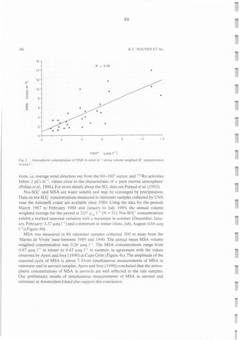
86
46 B. C. NGUYEN ET AL.
16
R = 0.78
14 •
12 €"
1
E 10
0 E
-=- 8
Cil ::i: 6 Cl
4
2
0 0 2 4 6 8 1 0 1 2
Fig. 3 . Atmospheric concentration of OMS in nmol m -' versus volume weighted H- concentration in µeq 1-1
•
tians. i.e. average wind direction out from the 60- 180° sector, and 222 Rn activities below 2 pCi m-3, values close to the characteristic of a ·pure marine atmosphere· (Polian er al.. 1986). For more details about the SO~ data see Putaud et al. ( 1992).
Nss-SOt and MSA are water soluble and may be scavenged by precipitation. Data on nss-SOt concentrations measured in rainwater samples collected by UVA near the Antonelli cracer are available since 1980. Using the data for the periods March 1987 to February 1988 and January to July 1989, the annual volume weighted average for the period is 2.07 µ
0Y 1- 1 (N = 51 ). Nss-SOt concentrations
exhibit a marked seasonal variation \vith a maximum in summer (December. Janu-ary, February: 3.37 µeq 1- 1
) and a minimum in winter (June. July. August: 0.66 µeq 1- 1) (Figure 4b).
MSA was measured in 86 rainwater samples collected 300 m away from the ·Martin de Viviès· base between 1989 and 1990. The annual mean MSA volume weighted concentration was 0.20 µeq 1- 1
• The MSA concentrations range from 0.07 µeq 1- 1 in winter to 0.45 µeq 1- 1 in summer. in agreement with the values observed by Ayers and Ivey ( 1990) at Cape Grim (Figure 4c). The amplitude of the seasonal cycle of MSA is about 7. From simultaneous measurements of MSA in rainwacer and in aerosol samples, Ayers and lvey ( 1990) concluded that the atmos-pheric concentrations of MSA in aerosols are well reflected in the rain samples. Our preliminary results of simultaneous measurements of MSA in aerosol and rainwater at Amsterdam Island also support this conclusion.
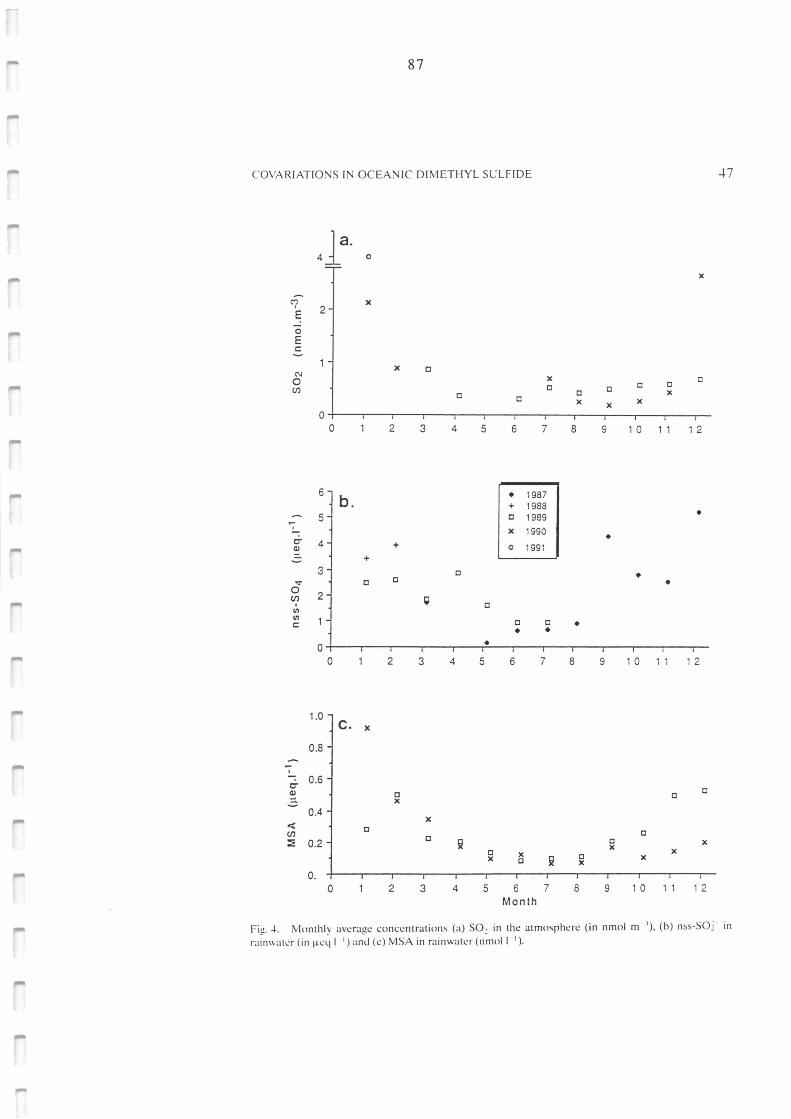
87
COVARIATIO NS IN OCEANIC DIMETHYL SULFIDE -l- 7
41a. 0
X
<7 X
E 2
0
E C
X C N 0 X C (/) C C C Cl
Cl Cl X Cl X X
X
0 0 2 3 4 5 6 7 8 9 1 0 11 1 2
6 b. • 1987
+ 1988 5 Cl 1989 •
";--: X 1990 • C" 4 ~
+ 0 1991 +
3 Cl Cl • st Cl • 0
2 (/) l;I ' Cl Ill Ill C Cl Cl • • •
0 • 0 2 3 4 5 6 7 8 9 1 0 11 1 2
1.0 c. X
0.8
';--: 0.6 C" Cl) Cl Cl
Cl X
0.4 X
< Cl (/) Cl
~ 0.2 C Il Cl
X X
Cl X X X Cl Il Cl X
X
o. 0 2 3 4 5 6 7 8 9 1 0 11 1 2
Mon th
Fig. 4. Montilly average concentrations (a) SO, in the atmosphere (in nmol m '), (b) nss-SO_i- in
rainwat..:r (in r1..:q 1 1) anu (c) MSA in rainwatcr (nmol l 1 ).
88
48 B. C. NGUYEN ET AL.
3.4. Comparison Between the Amplitude of the Seasonal Cycle of DMS and its
Oxidation Products
We have observed that the seasonal amplitude of MSA (summer/ winter ratio: 7) is similar to that of S0 2 (6 to 9). Moreover, the amplitude of the mean seasonà.l cycle of atmospheric OMS concentrations measured over more than 4 year period (January 1984-August 1985; March 1987-February 1988 and August 1988-Oecember 1990) is also similar to that of MSA and S0 2 (about 7 during the whole period and 9 during the period with S0 2 data). These observations under pure oceanic conditions suggest that atmospheric OMS can account for the observed MSA and S0 2 values at Amsterdam Island. The linearity between OMS and MSA at Amsterdam Island is in good agreement with that obtained by Ayers et
al. ( 1990) at Cape Grim. These authors also observed a seasonal amplitude of nss-SOt in the sub-micro-
meter-aerosol, but it is about a factor of 2 smaller than that of the OMS and MSA and they conclude that this may imply the existence of another source of aerosol sulfur in addition to OMS (oxidation of other gaseous sulfur species or long-range transport of sulfate). The seasonal amplitude of nss-SOt in precipitation on Amsterdam Island appears to be somewhat lower (summer/ winter ratio of 5) rela-tive to those of OMS and MSA. It is difficult. however, to assess the significance of these differences since the seasonal cycles for different species plotted in Figures 2 and 4 do not represent coïncident sampling periods. Significant interannual varia-bility is evident in these data. and in longer term data records for the chemical com-position of precipitation at the site (Moody et al., 1991 ). The long distance trans-port of anthropogenic sulfur from Africa does appear to contribute on occasion to elevated concentrations of nss-SOt in precipitation on Amsterdam Island (Moody et al.. 1991 ). The impact is most evident during austral spring (September and October), however. and as such. \vould not be expected to influence summer/ winter amplitudes in nss-SOt to a large degree.
A number of physical factors may also contribute to differences in the seasonal amplitudes of atmospheric sulfur species in the region. Temperature dependence in the branching ratio for production of MSA and H 2SO4 from OMS oxidation (e.g. Ayers et al., 1986) could con tri bute to greater seasonal amplitudes in nss-SO t relative to MSA. More rapid homogeneous oxidation rates of S0 2 to H 2S0 4 during the summer relative to the winter may lead to greater seasonal amplitudes in nss-SO t relative to S0 2• Conversely. the more efficient heterogeneous oxidation of S0 2 associated with higher concentrations of sea-salt aerosols (e.g. Sievering et al.,
1991) during the winter could have the revearse influence on relative differences in seasonal amplitudes for S0 2 and nss-SOt. MSA and nss-SOt may exhibit differ-ences in their particle size distributions (e.g. Pszenny, 1991) which suggests that they may experience different dry deposition velocities. Since particle size distribu-tions for aerosol over the southern Indian Ocean are expected to vary seasonally (e.g., see Erickson and Duce. 1988). the relative atmospheric lifetimes for MSA
89
COVARIATIONS IN OCEANIC DIMETHYL SULFIDE 49
and nss-SO t against dry deposition may also vary seasonally. Ali of these factors complicate the direct interpretation of relative differences in seasonal amplitudes between species. The similarities in seasonal cycles between OMS and its oxidation products suggest that these species may originate primarily from a common marine biogenic source. There are substantial uncertainties in this analysis, however, and our observations do not preclude the presence of small but finite concentrations of anthropogenic sulfur at this remote location. Such an influence would be expected to dampen the seasonal amplitude for nss-sor relative to the other sulfur species.
3.5. DMS Cycle above Amsterdam Island
In order to arrive at any conclusions about the contribution of OMS to rain acidity, the downward flux of sui fur and the oceanic OMS flux have to be compared. Figure 5 schematizes the mechanis of OMS production in seawater and its oxidation path-ways in the atmosphere. In surface seawater (0-100 m) the major sources of OMS are phytoplankton metabolism. phytoplankton grazing by zooplankton. and finally phytoplankton senescence (Nguyen et al .. 1988; Oacey and Wakeham, 1986: Belviso et al., 1991 ). In Figure 5. we also summarize the results and estimates of individual fluxes and concentrations of atmospheric sulfur compounds in the southern Indian Ocean. The OMS removal rate is calculated from a simple steady-state box mode! similar to those used by several authors (Andreae. 1986; Berres-heim et al .. 1990; Pszenny et al .. 1989; Nguyen et al.. 1990; Bates et al.. 1990). In this mode!. a I km high boundary layer is considered (Toon et al .. 1987; Yu, 1988) and assumed to be vertically well mixed. From our data on OMS concentrations in the atmosphere at Amsterdam Island. the mean atmospheric OMS concentration is ..J. .3 nmol m--1, equivalent to an integrated-column concentration of 4.3 µmol m -2 in the mixed layer. The OMS tlux from sea-to-air is calculated from gas exchange models (Liss. 1973) using OMS concentrations in seawater and an exchange coeffi-cient (K,J dependent upon windspeed (Liss and Merlivat, 1986). Ouring the 1987-1989 period. the annual average OMS tlux is calculated at 3.0 µmol m-2 d- 1
•
We note that a large uncertainty exists in the calculation of the exchange coefficient and that the different approaches can give results differing by a factor as large as 1.8 (Erickson et al .. 1990). The calculated OMS flux is therefore given with an uncertainty of a factor at least of 2.
For the annual wet deposition of MSA, assuming a volume weighted mean MSA concentration of 0.20 µeq 1- 1 and an annual mean rainfall of 113 cm (during the 1987-1990 period). a figure of 0.6 µmol m-2 d- 1 is obtained. In this area. the annual mean atmospheric concentration of S0 2 is 0.7 nmol m-.1. i.e. 0.7 µmol m-2
for a I km air column. With a deposition rate of 1.0 cm Ç 1 (Sievering et al .. 1989) we obtain a removal rate by dry deposition of 0.7 µmol m-2 d - 1
• For the annual mean deposition of nss-SOt, using the mean nss-SOt concentration of 2.07 µeq 1- 1 and an annual mean rainfall of 113 cm, a wet deposition of 3.2 µmol m -2 d- 1 is
obtained. On Amsterdam Island. precipitation occurs about 241 days a year. Dry
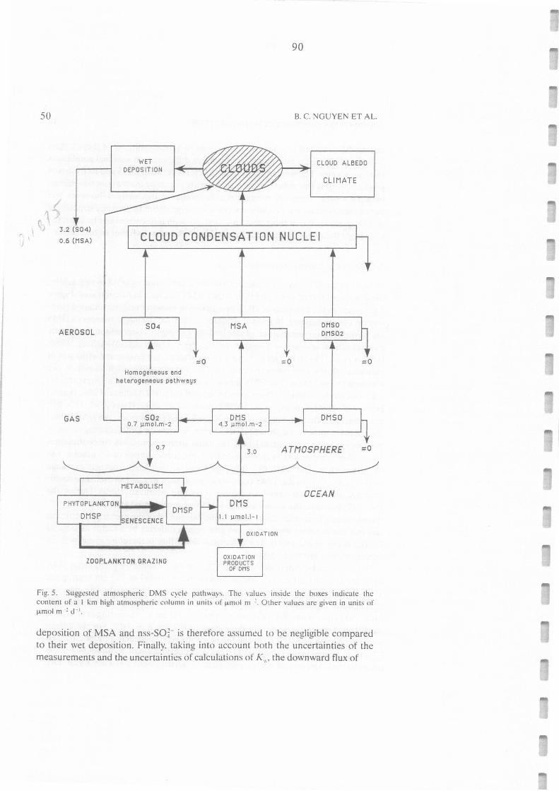
50
/ 'l-"
90
B. C. NGUYEN ET AL.
CLOUD ALBEDO
CLIMATE
• Q) 3.2 (S04) r 1 CLOUD CONDENSATION NUCLEI /
1 0.6 (MSA)
AEROSOL
GAS
S04
:0 Homogeneous end
heterogeneous pcthwcys
S02 0.7 µmol.m-2
0.7
METABOLISM
PHYTOPLANKTON+----1•~ DMSP
.___...,O,_M_s_P _ __,SENESCENCE '--~--'
ZOOPLANKTON GRAZING
MSA
DMS 4.3 µmol.m -2
3 .0
DMS 1.1 µmol.1-1
OXIDATION
OXIDATION PRODUCTS
OF OMS
=O
DMSO DMS02
DMSO
A Tl105PHERE
OCEAN
:0
=O
Fig. 5 . Suggested atmospheric DMS cyck pathways. The value~ inside the hoxes indicate the content of a I km high atmospheric column in units of µmol m :_ Otht::r values are given in units of µmol m 1 d - 1•
deposition of MSA and nss-SOJ- is therefore assumed to be negligible compared to their wet deposition. Finally. taking into account both the uncertainties of the measurements and the uncertainties of calculations of K ... , the downward flux of
91
COVARIATIONS IN OCEANIC DIMETHYL SULFIDE 51
sulfur (4.5 µmol m-2 d- 1) cou Id match the oceanic OMS flux (3.0 µmol m-2 d- 1 ).
Table II shows the contribution of OMS oxidation products (MSA and nss-SOt) to the AEX and the total acidity. Since the measured concentration of H + is simply the residual of an acid-base balance involving a variety of acids neutralized by alkalis (ammonia and nss-Ca2+), the ratios presented in this table should be viewed as an upper limit for the contribution of the individual compounds to the acidity of rainwater. Based on Galloway and Gaudry"s (1984) measurements. we estimate that ammonium and nss-Ca 2+ can contribute about 20% to the total cation budget. Thus the ratios in Table II could be overestimated by about 20%. Table II reveals that nss-SOt and MSA should be responsible for about 55% of the acidity in excess in rainwater and approximately 40% to the total rainwater acidity at Amsterdam Island. These results can be compared with those of Moody er al.
( 1991 ). Their calculation of the potential contributions of different acids to original acidity (defined as: H ~ + seasalt alkalinity + nss nss-Ca 2+ + NH;) indicate that on average H 2SO-1 accounted for 25% of the original acidity in precipitation sampled between 1980 and 198 7. There was however, considerable variability in the relative contribution of H 2SO -1 with values ranging from O to 7 5% for individual precipita-tion events. Severa! other acids were also found to be important with carboxylic acids. hydrochloric acid. and nitric acid contributing on average 25, 25. and 12%. respectively. of the original acidity.
4. Conclusion
The simultaneous measurement of rain acidity and OMS and its oxidation products at Amsterdam Island allow us to recognize, for the first time, a coherence between the seasonal cycles of oceanic and atmospheric concentrations of OMS, and rain acidity. Atmospheric concentrations of S0 2 and wet deposition of MSA present seasonal cycles similar to that of atmospheric OMS and with quite similar ampli-tudes. indicating a linearity in the seasonal cycles of OMS. MSA. and S0 2•
We have shown that within the uncertainties of the measurements and the uncer-tainties of calculations of Kw, the downward flux of sulfur could match the oceanic OMS flux. A comparison between the OMS oxidation product fluxes (nss-SOt, MSA). the acidity in excess and the total acidity, allow us to make an upper esti-mate of the OMS contribution: approximately 55% to the acidity in excess and about 40% to to tal acidity in rain.
Acknowledgements
We thank J . C. Ouplessy, G. Lambert, S. Belviso, J. L. Moody, and A. McTaggart for helpful comments ami C. Harris for help in preparing this manuscript. This work was supported by the Territoire des Terres Australes et Antarctiques Fran-çaises. the Centre National de la Recherche Scientifique and Commissariat à !"Energie Atomique. This is a contribution to the Global Precipitation Chemistry
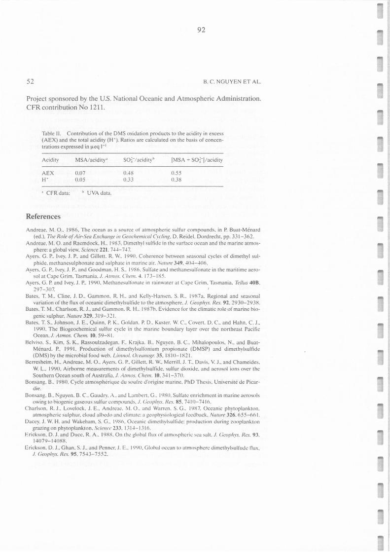
92
52 B. C. NGUYEN ET AL.
Project sponsored by the U.S. National Oceanic and Atmospheric Administration. CFR contribution No 1211.
Table II. Contribution of the OMS oxidation products to the acidity in excess (AEX) and the total acidity (H·). Ratios are calculated on the basis of concen-trations expressed in µeq 1-1
Acidity
AEX H+
·' CFRdata;
References
MSA/acidity"
0.07 0.05
" UVAdata.
SOt/acidityh
OA8 0.33
IMSA + SOtl/acidity
0.55 0.38
Andreae. M. O .. 1986, The ocean as a source oî atmospheric sulfur compounds. in P. Buat-Ménard (ed.). The Rote of Air-Sea Exchange in Geochemical Cycling. D. Reidel. Dordrecht. pp.331-362.
Andreae. M. O. and Raemdock. H .. 1983. Dimethyl sulfide in the surface ocean and the marine atmos-phere: a global view. Science 221. 7-+-+-7-+ 7.
Ayers. G. P .. lvey. J. P .. and Gillett. R. W .. I 990. Coherence between seasonal cycles oî dimethyl sul-phide. methanesulphonate and sulphat<! in marine air. ilia111re 349. -+0-+--+06.
Ayers. G. P .. lvey. J. P .. and Goodman. H. S .. 1986. Sulfate and m<!thanesulfonate in th<! maritime aero-sol at Cape Grim. Tasmania. /. A1111os. C/11.'111. 4. 17 3-185.
Ayers. G. P. and lvey. J. P .. 1990. Methanesulfonate in rainwater at Cape Grim. Tasmania. Tell11s 40B. 297-307.
Bates. T. M .. Cline. J. D .. Gammon. R. H .. and Kelly-Hansen. S. R .. 1987a. Regional and seasonal variation of the flux of oceanic dimethylsulfide to the atmosphere. /. Geophys. Res. 92. 2930-2938.
Bates. T. M .. Charlson. R. J .. and Gammon. R. H .. 1987b. Evidence for the climatic roi<! of marine bio-genic sulphur. Nawre 329, 319-321.
Bates. T. S .. Johnson. J. E .. Quinn. P. K.. Goldan. P. D .. Kuster. W.C.. Covert. D. C.. and Hahn. C. J .. 1990. The Biogeochemical sulfur cycle in the marine boundary layer over the northeast Pacifie Ocean. /. Armas. Chem. 10. 59-81.
Belviso. S .. Kim. S. K .. Rassoulzadegan. F.. Krajka. B.. Nguyen. B. C.. Mihalopoulos. N .. and Buat-Ménard. P .. 1991. Production of dimethylsulfonium propionate (DMSP) and dimethylsulfide (OMS) by the microbial food web. Li111nol. Ocewwgr. 35. 1810-1821.
Berresheim, H .. Andreae, M. O .. Ayers. G. P .. Gillett. R. W.. Merrill. J. T.. Davis. V. J .. and Chameides. W. L.. 1990. Airborne measurements of dimethylsullïde. sulfur dioxide. and aerosol ions over the Southern Ocean south of Australia. J. A1111os. Chem. 10. 341-370.
Bonsang. B .. 1980. Cycle atmosphérique! du soufre d"origine marine. PhD Thesis. Université de Picar-die.
Bonsang. B .. Nguyen. B. C.. Gaudry. A.. and Lambert. G .. 1980. Sulfate enrichmcnt in marine acrosols owing to biogenic gaseous sui fur compounds. /. Cieoph1·s. Ues. 85. 7410-7416.
Charlson. R. J .. Lovclock. J. E .. Andr<!ae. l\·I. O .. ,md Warren. S. G .. 1987. Occanic phytoplankton. atmospheric sulphur, cloud albedo and climatc: a geophysiological feedhack. Nm11re 326. 655-661.
Dacey. J. W. H. and Wakeham. S. G .. 1986. Oc.:eanic dimcthylsulfidc: production du ring zooplankton grazing on phytoplankton. Science 233. 1314-1316.
Erickson. D. J. and Duce. R. A .. 1988. On the global !lux of atmosphcric sca sait./. Geophys. Ues. 93. l 4079-14088.
Erickson. IJ. J .. Ghan. S. J .. and Pcnn<:r. J. E .. 1990, Global occan to atmŒphcrc dimethylsulfudc !lux. J. Geophys. Res. 95. 7543-7552.
93
COVARIATIONS IN OCEANIC DIMETHYL SULFIDE 53
Galloway. J. N. and Gaudry. A .. 1984. The composition of precipitation on Amsterdam island . Indian Ocean. Amtus. Em"irun. 18. 2649-2656.
Gibson. J. A. E .. Garrick. H. R. Burton. H. R., and McTaggart. AR .. 1990. The alga Phaeoc_rnis
poucheti and dimethylsulfide in Antarctic coastal waters. 1'vlarine Biot. 104. 339-346. Keene. W.C.. Pszenny. A. A. P .. Galloway. J. N .. and H awley. M. E .. 1986. Seasonal corrections and
interpretation of constituent ratios in marine precipitation. J. Geophys. Res. 91. 66-17-6658 . Likens. G. E.. Keene. W.C .. Mi ll er. J. M .. and Galloway, J. N .. I 987, Chemistry of precipitation from a
remote. terrestrial site in Australia. J. Geophys. Res. 92. 13299-13314. Liss. P. S .. 197 3. Processes of gas exchange across an air-water interface. Deep Sea Res. 20. 221-2 38. Liss. P. S. and Merlivat. L.. 1986. in P. Buat-Ménard (ed.). The Rote of Air-Sea Exclzange in Gevchemi-
cat c_,-cling. D. Reidel. Dordrecht. pp. 113-127. Lm·elock. J. E .. Maggs. R. J.. and Rasmussen . R. A . 1972 . Atmospheric dimethylsulfide and the global
sui fur cycle. Na111re 237. -152-453. Mihalopoulos. N .. Nguyen. B. C.. and Beh"iso. S .. 1988. Dimethyl sulfide in the Somali upwelling area.
Chem. Geutogy70(1 ! 2). 95. l'vloody. J. L.. Pszenny. A. A. P .. Gaudry. A .. Keene. W.C.. Galloway. J. N .. and Polian. G .. 1992. Pre-
cipitation composition and its variability in the southern Indian Ocean: Amsterdam Island. 1980-1987. J. Geuph_n. Res. (in press).
Nguyen. B. C.. Bonsang. B .. and Lambert. G .. 197-1. The atmospheric concentrations of sulfur dioxide and sulfate aerosols over Antarctica. Subantarctic areas and oceans. Tellus 26. 2-11-2-17.
Nguyen. B. C .. Gaudry. A.. Bonsang. B .. and Lambert. G .. 1978. Reevaluation of the role of dimethyl sulphide in the sulphur hudget. J\"(1(11re 275. 637-639.
Nguyen. B. C.. Bonsang . B .. and Gaudry. A .. 1983. The mie of the ocean in the global atmospheric su lfur cycle. J. Geuphys. Res. 88. 10903-10914.
Nguyen. B. C.. Belviso. S .. Mihalopoulos. N .. Gostan . J.. and Nival. P .. 1988. Dimethylsulfude produc-tion du ring natural phytoplankton hlooms. Marine Chem. 24. 133-141.
Nguyen. B. C.. Mihalopoulos. N .. and Beh"iso. S .. 1990. Seasonal variation of atmospheric dimethvl-su lfide at Amsterdam Island in the southern lndian Ocean. J. Aunos. C/1em. 11. 123-1-13.
Polian . G .. Lambt:rt. G .. Ardouin. B .. and Jégou. A .. 1986. Long range transport of continental radon in subantarctic areas. Te/lus 388. 178-189.
Putaud. J. P .. Mihalopoulm. N .. Nguyen . B. C .. Campin. J . M .. and Belviso. S .. 1992. Seasonal varia-tions of atmospheric sulfur dioxide and dimethylsulfide concentra tions at Amsterdam Island in the Southern lndian Ocean. J. Atmus. C/1em .. in press.
Pszrnny. A. A. P .. Maclntyre. F .. and Duce. A .. 1982. Sea sa it and acidity of marine rain on the wind-ward coast of Samoa. Gt'opl,_n. Res. Leu. 9. 751-75-1.
Pszenny. A. A. P.. Ca~telle. A. J.. Galloway. J. N .. and Duce. R. A .. l 989. A study of the sulfur cycle in the Antarctic marine boundary layer. J. Geoph_vs. Res. 94. 9818-9830.
Pszenny. A . A. P .. 1992. Parricle size distributions fo r methanesulfonate in the tropical Pacifie marine boundary layer. J. , \1111os. Chem. (in press).
Saltzman. E. S .. Savoie. D. L.. Zika. R. G .. and Prospt:ro. J. M .. l 983. Methanesulfonic acid in the marine atmosphere. J. Gmphys. Res. 88. 10897-10902.
Shaw. 1983. Bio-controlled thcrmostasis inrnlving the sulfur cycle. Climaric Change 5. 297-303. Sien:ring. H .. 13oatman. J.. Luria. M .. and Van Valin. C. C .. 1989. Sulfur dry deposition over the
western North Atlantic : the mit: of cnarse aerosol particles. Te/lus 418. 338-3-13. Sievering. H .. Boatman. J.. Galloway. J.. Keem:. W .. Kim . Y.. Luria. M .. and Ray. J.. 1991. Hetern-
g.:neo us sui fur conversion in sea-sa lt aemsol particles: The mie of aemsol water content and size distrihution . .- 111110.1. E111"iro11. 25A. 1-179-1-187.
Toon. O. 13 .. Kasting. J. F.. Turco. R. P .. and Liu. M. S .. 1987. The su lfur cycle in the marine atmos-phcre. J. Geoph,·s. /?es. 92. 943-963.
Turn<:r. S. M .. Malin. G .. Li,s . P. S .. Harbour. D. S .. and Holligan . P. M .. 1988. The seasnnal variation of dimcthy l sullïdc and dimcthylsulfoniumpmpionate concen trations in nearshore waters. Li111110/.
OcC'wwgr. 33(3). J(i-1-375. Yu. T. W.. l 9XX. A method for det<:rmining .:quivaknt depths of the atmospheric boundary layer ov<:r
th<:oceans.J. (i<'opl,_1·s. t?es. 93. 3(i55-3(i(il.

95
Conclusion
Les variations saisonnières du flux océan-atmosphère de DMS, liées aux cycles d'activité
biologique du plancton, sont reflétées par les variations saisonnières de SO2, MSA et nss-
SO4. Ceci suggère que le SO2 présent dans l'atmosphère marine est principalement produit
par l'oxydation du DMS, ce que confirment les covariations à court terme des concentrations
de ces composés pendant deux mois d'été. Ces résultats montrent également que les variations
de production de DMS ont un impact sur la concentration en composés soufrés de
l'atmosphère, ce qui constitue une première étape dans l'hypothèse de l'effet du DMS sur la
production de noyaux de condensation .
La comparaison du rapport des concentrations SO2/DMS (moyenne de 0.2) avec les
résultats d'un modèle de boite photochimique décrivant les processus de formation et de
destruction de SO2 selon des paramétrisations récentes montre qu'en moyenne 70% du DMS
serait oxydé en SO2. Cependant, la vitesse d'oxydation de DMS par OH considérée dans ce
modèle semble faible puiqu 'elle correspond à un temps de vie de DMS vis-à-vis de son
oxydation par OH de l'ordre de 2 à 7 jours, suivant la concentration de OH qui varie d'un
facteur 4 entre l'été et l'hiver. Ceci pourrait provenir d'une sous-estimation de la constante
de vitesse (koH)de la réaction DMS + OH (Hynes et al., 1986), ou du champ de OH obtenu par
un modèle 3-D (M. Kanakidou, communication personnelle), qui n'a pas encore été validé
par des mesures dans la zone géographique de l'île Amsterdam. Il est aussi probable que des
radicaux autre qu'OH (e.g. NO3) contribuent à l'oxydation du DMS. En considérant un vitesse
d'oxydation du DMS plus élevée, correspondant à un temps de vie du DMS plus en accord avec
la littérature (e.g . 36 heures; Andreae, 1986), aurait conduit à une estimation de la
fraction de DMS oxydée en SO2 beaucoup plus faible, de l'ordre de 25%.
Parallèlement, la comparaison du flux océan-atmosphère de DMS et du dépôt humide de
MSA montre qu'environ 20% du DMS est oxydé en MSA. Mais rappelons qu'en tenant compte
de la réévaluation du coefficient d'échange océan-atmosphère permettant de calculer le flux
96
de DMS (cf chapitre 1 }, l'estimation de la fraction de DMS oxydée en MSA serait réduite à
::::10% .
L'acidité des précipitations covarie avec les concentrations de composés soufrés et la
contribution des acides MSA + H2SO4 à l'acidité en excès de l'eau de pluie est d'environ 50%.
L'acidité naturelle des précipitations n'affecte évidemment pas l'environnement dans la zone
de l'île Amsterdam. Cependant, la grande majorité des espèces formant les noyaux de
condensation dans les nuages sont des acides (Twomey, 1971). Ces acides sont dans
l'atmosphère partiellement neutralisés par réaction avec l'ammonniac (NH3) ou le chlorure
de sodium (NaCI) d'origine marine( 1). Le rapport entre les concentrations des produits
d'oxydation du DMS (MSA et H2SO4) et les ions H+ ne permet donc pas de calculer leur
contribution à l'acidité "originelle" des aérosols, qui permettrait de chiffrer l'importance
des composés soufrés par rapport aux acides nitrique, organiques, etc, dans la formation des
noyaux de condensation. Il suggère néanmoins une contribution significative de ces produits à
la formation de CCN.
Cependant, s'il se confirmait que la fraction de DMS oxydée en SO2 et MSA est de l'ordre
des limites inférieures de nos estimations (respectivement 25% et 10%), il resterait une
part importante de DMS pour former d'autres produits. Le peu de mesures de DMSO et
DMSO2 publiées (Watts et al., 1987a) indiquant que ces produits sont très minoritaires,
celles-ci impliqueraient que le chemin réactionnel conduisant du DMS à l'acide sulfurique
via SO3, sans passer par la formation de SO2, serait important. Cette hypothèse, récemment
émise par Bandy et al. (1992) pour interpréter des mesures effectuées dans l'océan
Atlantique, signifierait que la production de H2SO4 en phase gazeuse est importante, alors
que ce chemin réactionnel n'est jamais pris en compte dans la modélisation du cycle du
soufre. Dans l'optique de la formation de noyaux de condensation, ce résultat serait très
ïmportant: la nucléation bimoléculaire H2SO4 - H2O en phase gazeuse conduit à la formation
de nouvelles particules, alors que l'oxydation de SO2 en H2SO4, qui s'opère majoritairement
dans des aérosols préexistants, ne contribue qu'à la croissance des particules préexistantes.
1 Cette réaction conduit à l'émission de chlorure d'hydrogène (HCI) gazeux.
97
CC Il-il A IP Il T IFUE Il Il Il
SULFURE DE DIMETHYLE, AEROSOLS ET NOYAUX DE CONDENSATION

99
SULFURE DE DIMETHYLE, AEROSOLS ET NOYAUX DE CONDENSATION.
INFLUENCE DES EMISSIONS DE SULFURE DE DIMETHYLE ET DES COMPOSES SOUFRES PARTICULAIRES SUR LA POPULATION DE NOYAUX DE CONDENSATION.
Comme il l'a été rappelé précédemment, les produits d'oxydation atmosphérique du DMS à
caractère acide (S02, MSA, H2S04) contribuent à la formation des noyaux d'AïtkenOl (CN).
La nucléation bimoléculaire homogène en phase gazeuse des acides MSA et H2so4 donne en
effet naissance à des "nouvelles particules" dont le diamètre est de l'ordre de 1 o-3 µm, qui
ne contiennent que quelques milliers de molécules. Ces particules sont succeptibles de
croître jusqu'à la taille de CN par plusieurs processus dont l'incorporation d'autres
molécules d'acides (ou d'ammoniac), l'absorption de S02 qui va subir une oxydation
hétérogène dans la particule, et la collision avec d'autres particules existantes conduisant à
leur agglomération. La totalité de la population de CN ne joue pas un rôle dans la formation
des gouttelettes d'eau des nuages: il ne peuvent servir de germes de condensation que si leur
rayon atteint une taille critique, dépendant de la sursaturation en vapeur d'eau et de la
composition chimique de la surface de la particule. Les CN présentant cette caractéristique
sont appelés noyaux de condensation(2) (CCN). Les CCN sont indispensables à la formation des
gouttelettes dans les nuages stratiformes de basse altitude où la convection n'est pas assez
forte pour entraîner la vapeur d'eau à des altitudes suffisamment élevées(3) pour qu'elle
donne des cristaux de glace. Leur concentration peut influencer l'albédo de l'atmosphère
suivant plusieurs processus découlant de la modification du spectre de taille des gouttelettes
dans les nuages (Figure 3.a.). Par exemple, dans un nuage où le contenu en eau liquide serait
fixé, une augmentation du nombre de CCN conduirait à la formation de gouttelettes plus
1 On appelle noyaux d'Aïtken (en anglais condensation nuclei, CN) toute particule assez grosse pour être ·détectée par un compteur de noyaux. Typiquement, ces appareils détectent 100% des particules dont le rayon est supérieur à 0.01 µm, leur efficacité décroissant sous cette limite jusqu'à O pour pour les particules d'un diamètre de 0.005 µm.
2 Le principe de mesure des CCN est analogue à celle des CN, mais la chambre de nucléation contient de la vapeur d'eau dont la sursaturation est réglable: la concentration de CCN mesurée dépend donc de la sursaturation employée.
3 .. . pour que la température suffisament basse: il existe classiquement dans les nuages de l'eau surfondue jusqu'à des températures inférieures à -10°C. En laboratoire, de l'eau liquide a été amenée à - 40°C (Caro, 1992).
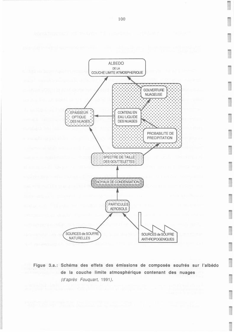
Figue 3.a.:
~ . . . . . . ,. AA,EPAISSEUR <- OPTIQUE
100
ALBEDO DELA
COUCHE LIMrTE ATMOSPHERIQUE
: A'.DES NUAGES: A
CŒTENUEN EAU LIQUIDE DES NUAGES
Schéma des
A A_.A_A_A_A_A__,,A__,,A__,,A-. A ,_ A A A A A ,_ A ,_
A A A A A A A A A A A A A A A A A A A A
A A A A A A A A A A A A A A A A A A A A PROBABILITE DE A A A A A A A A A A ,. : A:,.:,.: A:,.: A:,.:,.: A: PRECIPITATION ,. A AAAAAAAAAAAAAAAAA,_A,_-;::..,....,....,....,.,,.....,....,....,.,....~A A
A A A
: : : : : : : SPE°CTRE0
DE TÂILLÊ::::: ,,.,,,. '•'•' : : : : : : : DES GOUTTELETTES::::! •,:,:•!·,·,·,·,·,···········!•!•'
effets des émissions de composés soufrés sur
contenant des nuages de la couche limite atmosphérique
(d'après Fouquart, 1991 ).
l'albédo
101
nombreuses (mais plus petites) dont la surface totale est plus grande(4), ce qui accroît
l'albédo du nuage. Autre phénomène entraîné par la diminution du rayon moyen des
gouttelettes: la limitation du risque de précipitation, qui augmente la durée de vie des nuages
et donc, globalement, l'extension spatiale de la couche nuageuse.
Pour déterminer l'influence de différentes sources sur la formation de CCN, l'idéal serait
d'estimer la composition chimique individuelle des CCN, ce qui est encore difficilement
réalisable. Il est cependant possible de collecter les particules d'aéroso1(5) de rayon
supérieur à 0.01 µm sur des filtres dont le contenu en espèces solubles est analysable par
chromatographie ionique (Annexe 2). Mais on n'obtient alors que la composition chimique
moyenne de l'aérosol en terme de moles par unité de volume d'air et non pas la distribution
des particules suivant leur composition chimique.
La diversité des techniques d'analyse utlisées, présentant d'importantes différences de pas
de temps d'échantillonnage, et la multiplicité des étapes conduisant des espèces gazeuses à la
formation événtuelle de noyaux de condensation rendent l'influence des émission de composés
soufrés sur la population de CCN difficile à appréhender. Si la comparaison des cycles
saisonniers de composés soufrés (DMS et MSA) avec les variations saisonnières des
concentrations de CN et CCN observées à Cape Grim en Tasmanie (Ayers et al., 1991; Gras,
1990) montre un nette covariation entre ces paramètres, cette observation est bien sûr
insuffisante pour prouver une relation de cause à effet entre l'émission de DMS depuis
l'océan et la formation de CCN. Cependant, des résultats obtenus dans l'Atlantique sud,
présentés récemment par Andreae et al. (1993), mettent aussi en évidence des covariations
à court terme entre flux de DMS, concentration atmosphérique de DMS, population de CN et
de CCN et, de façon moins évidente, concentration de sulfates en excès dans les aérosols. Outre
que ces covariations constituent un indice supplémentaire du rôle du DMS dans la formation
de CCN, elles indiquent que cette production de noyaux de condensation peut être rapide. Ceci
4 A volume d'eau liquide constant, on calcule aisément que la surface totale des gouttes d'un nuage dépend de la racine cubique du nombre de gouttelettes.
5 Le terme d'aérosol est appliqué à toute population de particules de phase condensée (liquide ou solide) dont la vitesse de chute est inférieure à 1 cm.s· 1 . Les particules de rayon > 0.01 µm peuvent être collectés avec une efficacité de plus de 80% (Watts et al., 1987b) dans les conditions de haut régime utilisées dans ce travail.
102
n'est pas reproduit par les modèles de nucléation utilisant des conditions initiales décrivant
raisonablement la couche limite atmosphérique marine.
Bien qu'on ne parvienne pas encore totalement à modéliser la formation de CCN,
l'oxydation atmosphérique du OMS semble donc contribuer de manière significative à ce
processus au-dessus des océans de l'hémisphère sud. Mais dans l'hémisphère nord, vu les
flux considérables de SO2 émis par les régions industrialisées (cf Annexe 1), les composés
soufrés anthropogéniques ne dominent-ils pas la population de condensation ?
Pour apporter des éléments de réponse à cette question, nous avons participé à une
campagne océanographique (EUMELI 3) dans l'Atlantique tropical nord. Notre but était
d'étudier si des variations du flux de OMS pouvaient affecter sensiblement la concentration
en nombre de CN dans cette région du globe. Les zones traversées (eutrophes, mésotrophes,
oligotrophes) présentaient des niveaux de production primaire très contrastés. On pouvait
donc s'attendre à des productions de OMS différentes, dont les variations seraient comparées
à celles de la population de CN. Pour détecter l'advection de particules provenant d'autres
sauces, des mesures de traceurs tels que le 222Radon et la composition chimique des aérosols
ont été effectuées. Les résultats de cette expérience sont décrits dans l'article à paraître dans
Journal of Geophysical Research reproduit ci-après.
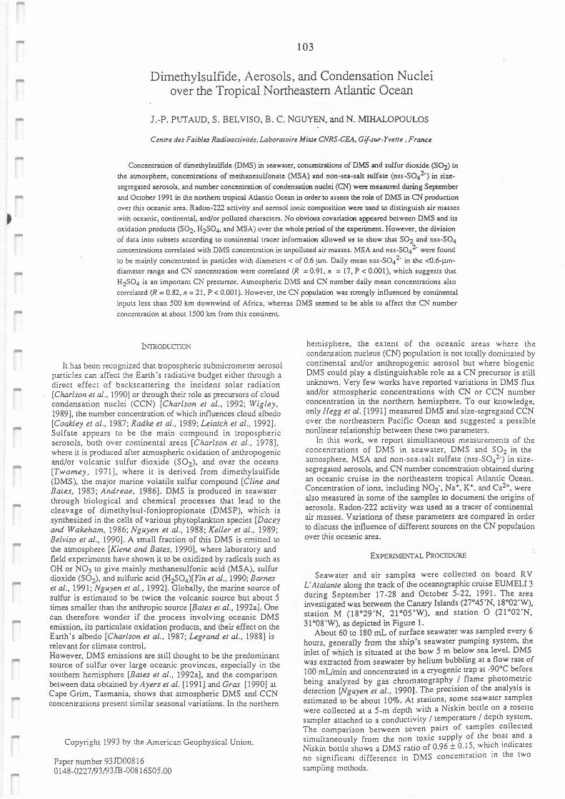
103
Dimethylsulfide, Aerosols, and Condensation Nuclei over the Tropical N ortheastem Atlantic Ocean
J.-P. PUT AUD, S. BEL VISO, B. C. NGUYEN, and N. MIHALOPOULOS
Cenlre des Faibles Radioactivités, lAboratoire MixJe CNRS-CEA, Gif-sur-Yvette, France
Concenlration of dimethylsulfide (DMS) in seawaler, concentrations of OMS and sulfur diox.ide (SOz) in
the atmosphere, concenlrations of methanesulfonate (MSA) and non-sea-salt sulfate (nss-soi·) in size-
segregaled aerosols, and number concenlration of condensation nuclei (CN) were measured during September
and October 1991 in the northem tropical Atlantic Ocean in order to assess the role of OMS in CN production
over this oceanic area. Radon-222 activity and aerosol ionic composition were used to dislinguish air masses
wüh oceanic, continental, and/or polluled characlers. No obvioos covariation appeared belween OMS and üs
oxidation produclS (SO2, H2SO4, and MSA) over the whole period of the cxperiment. However, the division
of dala imo subsets according to continenlal lracer information allowed us to show that SO2 and nss-S04 concentrations correlated with OMS concenlration in unpolluled air masses. MSA and nss-SO4
2· were found
to be mainly concentrated in particles with diameters < of 0.6 !.lm- Oaily mean nss-So/· in the <0.6-µm-
diameter range and CN concenlration were correlaled (R = 0.91, n = 17, P < 0.001), which suggests thal
HzSO4 is an imponant CN precursor. Atmospheric OMS and CN number daily mean concentrations also
correlaled (R = 0.82, n = 21, P < 0.001). However, lhe CN population was slrongly influenced by continent.al
inputs less lhan 500 km downwind of Africa, whereas OMS seemed to be able to affect lhe CN number
concentration al about l 500 km from this continenL
lNIRODl.iCTION
It has been recognized thac tropospheric submicromecer aerosol partiel es can affect the Earth 's radiative budget either through a direct effecc of backscactering the incident solar radiation [Charlson et al., 1990) or through cheir role as precursors of cloud condensation nuc!ei (CCN) [Charlson et al., 1992; Wigley,
1989], the number concentration of which influences c!oud aibcdo [Coakley et al., 1987; Radke et al., 1989; Leiatch et al., 1992]. Sulfate appears to be the main compound in tropospheric aerosols, both over continental areas [Charlson et al ., 1978). where it is produced after atmospheric oxidation of anthropogenic and/or volcanic sulfur dioxide (SO?), and over the oceans [Twomey, 1971 ], where it is deriv;d from dimethylsulfide (OMS), the major marine volatile sulfur compound [Cline and
Bates, 1983; Andreae, 1986). DMS is produced in seawater through biological and chemical processes that lead co the cleavage of dimechylsul-foniopropionate (DMSP), which is synthesized in the cells of various phytoplankton species [Dacey
and Wakeham, 1986; Nguyen et al., 1988; Keller et al., 1989; Belviso et al., 1990] . A small fraction of this DMS is emicced co the atmosphere [Kiene and Baies, 1990), where laboracory and field experirnents have shown it to be oxidized by radicals such as OH or NO3 co give mainly mechanesulfonic acid (MSA), sulfur dioxide (SO:z.), and sulfuric acid (H2SO4)[Yin et al., 1990; Barnes
et al., 1991; Nguyen et al., 1992). Globally, the marine source of sulfur is escirnaced to be twice the volcanic source but about 5 tirnes smaller than the anthropic source [Bates et al., 1992a). One can therefore wonder if the process involving oceanic DMS emission, its particulace oxidation products, and their effecc on the Earth's albedo [Charlson et al., 1987; Legrand et al., 1988] is relevant for clirnate control. However, DMS emissions are still thought ta be the predominant source of sulfur over large oceanic provinces, especially in the souchern hemisphere [Baies et al., 1992a), and the comparison between data obtained by Ayers et al. (1991) and Gras [I 990] at Cape Grim, Tasmania, shows chat atmospheric DMS and CCN concentrations present similar seasonal variations. In the norrhem
Copyright 1993 by the American Geophysical Union.
PJper nurnber 93JD008 l 6 0148-0227 f93f)3JB-00816S05.00
hemisphere, the extent of the oceanic areas where the condensation nucleus (CN) population is not cocally dominated by continental and/or anthropogenic aerosol but where biogenic DMS could play a distinguishable role as a CN precursor is still unknown. Very few works have reported variations in DMS flux and/or atmospheric concentrations with CN or CCN number concentration in the northem hemisphere. To our knowledge, only Hegg et al . (1991) measured DMS and size-segregated CCN over the northeastem Pacifie Ocean and suggested a possible nonlinear relacionship between these cwo parametcrs.
In this work, we report simulcaneous measurements of the concentrations of DMS in seawater, DMS and SO2 in the atmosphere, MSA and non-sea-salt sulfate (nss-Süi·) in size-segregated aerosols, and CN nurnber concentration obtained during an oceanic cruise in the northeascem tropical Atlantic Ocean. Concentration of ions, including NO3·, Na+, K+, and Ca2+, were also measured in some of the samples to document the origins of aerosols. Radon-222 activity was used as a tracer of continental air masses. Variations of these parameters are compared in order co discuss the influence of different sources on the CN population over this oceanîc area.
EXPER1ME1'.TAL PROCEDURE
Seawater and air samples were collected on board RV L'Atalante along the track of the oceanographic cruise EUMELI 3 during September 17-28 and October 5-22, 1991. The area investigated was bctween the Canary Islands (27°45'N, 18°02'W), station M (18°29'N, 21 °05 'W), and station O (21 °02'N, 31 °08 'W), as depicted in Figure 1.
About 60 ta 180 mL of surface seawater was sampled every 6 hours, generally from the ship's seawater pumping system, the inlet of which is situated at the bow 5 m below sea level. DMS was extracted from seawater by helium bubbling at a flow rate of 100 mL/min and concentraced in a cryogenic trap at -90°C before being analyzed by oas chromatography / flame photometric decection [Nguyen ei°al., 1990]. The prccision of the analysis is escimated to be about 10%. At stations, some scawater samples were collecced at a 5-m dcpch with a Niskin botcle on a rosetce sampler àttachcd to a conducrivicy / temperature / deplh system. The comparison between scven pairs of samplcs collected simultaneously from the non toxic supply of the_ bo~c ~d a Niskin botcle shows a DMS ratio of 0.96 ± 0.15. which md1cates no significant difference in DMS concentration in the two sampling methods.
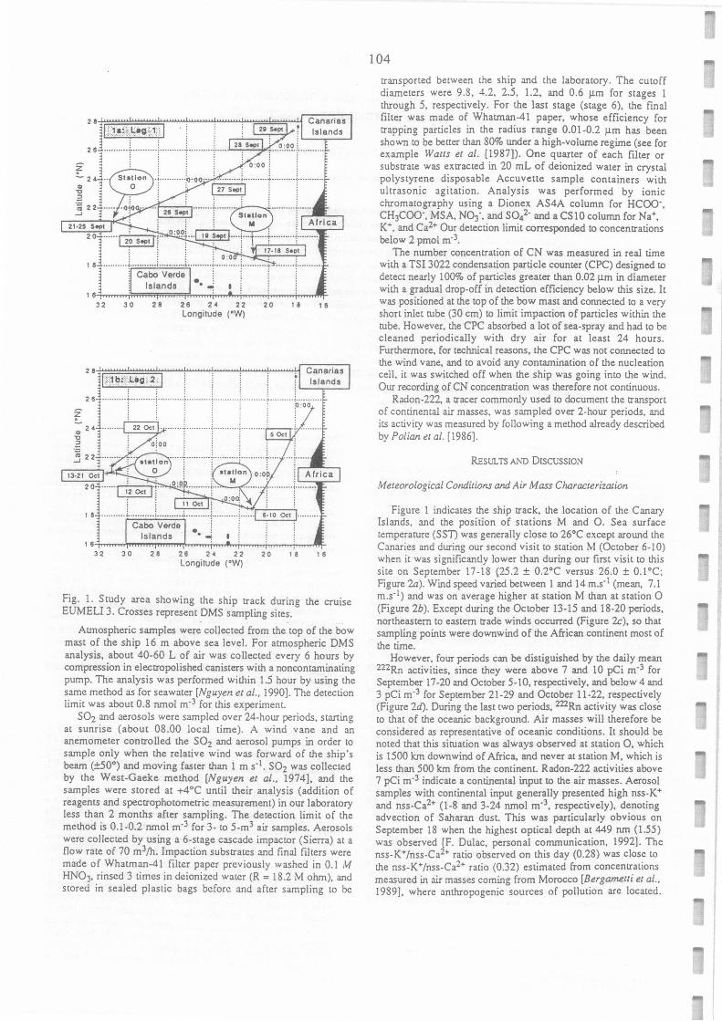
30
30 28 28 24 22 Longitude ("WJ
20 1 8
Canaries Islands
1 8
1 8
Fig. 1. Study arca showing the ship track during the cruise EUMELI 3. Crosses represent OMS sampling sites.
... Atmospheric samples were collected from the top of the bow
mast of the ship 16 m above sea level. For atmospheric OMS analysis, about 40-60 L of air was col!ected every 6 hours by compression in electropolished canisters with a noncontaminating pump. The analysis was perforrned within 1.5 hour by using the same method as for scawater [Nguyen et al., 1990]. The detection limit was about 0.8 nmol m·3 for this experiment.
SO2 and aerosols were sampled over 24-hour periods, starting at sunrise (about 08.00 local time). A wind vane and an anemometer controlled the SO2 and aerosol pumps in order to sample only when the relative wind was forward of the ship's beam (±50°) and moving faster than 1 m s·1• SO2 was collccted by the West-Gaeke method [Nguyen et al., 1974], and the samples were stored at +4°C until their analysis (addition of reagents and spectrophotometric measurement) in our laboratory less than 2 months after sampling. The detection limit of the method is 0.1-0.2 nmol m·3 for 3- ta 5-m3 air samples. Aerosols were collected by using a 6-stage cascade impacter (Sierra) at a flow rate of 70 m3/h. Impaction substrates and final filters were made of Whatman-41 filter papcr previously washed in 0.1 M HNO3, rinscd 3 times in dcionized water (R = 18.2 M ohm), and stored in sealed plastic bags beforc and after sampling ta be
104
transported between the ship and the !aboratory. The cutoff diameters were 9.8, 4.2. 2.5, 1.2, and 0.6 µm for stages 1 through 5, respective!y. For the last stage (stage 6), the final filter was made of Whatman-41 paper, whose efficiency for trapping partic!es in the radius range 0.01-0.2 µm has been shown ta be better than 80% under a high-volume regime (see for example Waus et al. (1987]). One quarter of each fi!ter or substrate was extracted in 20 mL of deionized water in crystal polystyrene disposable Accuvette sample containers with ultrasonic agitation. Analysis was performed by ionic chromatography using a Dionex AS4A column for HCOO·, CH3COO·. MSA. N03·, and soi· and a CS10 column for Na+, K+, and Ca2+ Our detection limit corresponded to concentrations below 2 pmol m·3.
The number concentration of CN was measured in real time with a TSI 3022 condensation parùcle counter (CPC) designed to detect nearly 100% of particles greater than 0.02 µm in diameter with a graduai drop-off in detection efficiency below this size. It was positioned at the top of the bow mast and connected to a very short inlet tube (30 cm) to limit impaction of particles within the tube. However, the CPC absorbed a lot of sea-spray and had ta be cleaned periodically with dry air for at least 24 hours. Furtherrnore, for technical reasons, the CPC was not connected ta the wind vane, and to avoid any contamination of the nucleation cell, it was switched off when the ship was going into the wind. Our recording of CN concentration was therefore not continuous.
Radon-222. a tracer commonly used ta document the transport of continental air masses, was sampled over 2-hour periods, and its activicy was measured by fol!owing a method already described by Polian et al. (1986].
RESL'LTS AND ÜISCUSSION
Meteorological Conditions and Air Mass Characterizarion
Figure 1 indicates the ship track, the location of the Canary Islands, and the position of stations M and O. Sea surface temperature (SSn was generally close ta 26°C except around the Canaries and during our second visit ta station M (October 6-10) when it was significantly !ower than during our first visit to this site on September 17-18 (25.2 ± 0.2°C versus 26.0 ± 0.1°C; Figure 2a). Wind speed varied between 1 and 14 m.s· 1 (mean, 7.1 m.s·1) and was on average higher at station M than at station 0 (Figure 2b). Except during the October 13-15 and 18-20 periods, northeastem ta eastem trade winds occurred (Figure 2c), sa that sampling points were downwind of the African continent most of the rime.
However, four periods can be distiguished by the daily mean 222Rn activiùes, since they were above 7 and 10 pCi m·3 for September 17-20 and October 5-10, respectively, and below 4 and 3 pCi m·3 for September 21-29 and October 11-22, respective!:( (Figure 2d). During the last two periods, 222Rn activity was close ta that of the oceanic background. Air masses will therefore be considered as rcpresentative of oceanic conditions. It should be noted that this situation was always observed at station 0, which is 1500 km downwind of Africa, and never at station M. which is less than 500 km from the continent. Radon-222 activities above 7 pCi m·3 indicate a continental input ta the air masses. Aerosol samples with continental input gencrally presented high nss-K+ and nss-Ca2+ (1-8 and 3-24 nmol m·3, rcspectively), denoting advection of Saharan dust. This was particularly obvious on September 18 when the highest optical depth at 449 nm (1.55) was observed [F. Dulac, persona! communication, 1992]. The nss-K+/nss-Ca2+ ratio observed on this day (0.28) was close to the nss-K+/nss-Ca2+ ratio (0.32) estimated from concentrations measured in air masses coming from Morocco (Bergame/li et al.,
1989], where anthropogenic sources of pollution arc located.
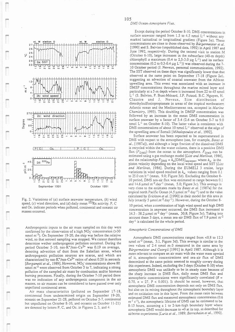
! P\ C! Oc. P C Oc.
1 1 1 1 1 1 1 1 1 1. t 1 1 1 1 1 1 1 1 1 1 1, 1,, 1 r,
- ..,.. N N N - - -- N
Seplember 1991 October 1991
Fig. 2. Yari~tion~ of ~a) surface sea_water temferarure, (b) wind speed, (c) wmd drrect1on, and (d) da1ly mean 2 2Rn activity. P, C and Oc. indicate periods when pollutcd, continental and oceanic air masses occurred.
Anthropogenic inputs to the air mass sampled on this day were confirmed by the observation of a high NOf concentration (>30 nmol m·3). On September 19-20, the ship was before the relative wind, so that acrosol sampling was stopped. We cannot therefore determine wether anthropogenic pollution occurred. Ouring the period October 5-10, nss-K•/nss-Ca2• was 0.19 on average, denoting advection of dust from the Sahelian areas, where anthropogenic pollution sources are scarce, and which arc charactcrized by nss-K•/nss-Ca2• ratios of about 0.20 in aerosols [Bergametti et al., 1989]. However, NO3• concentrations above 80 nmol m·3 were observed from October 5 to 7, indicating a strong pollution of the sampled air mass by combustion and/or biomass burning processes. Finally, during the October 7-10 period there was no indication of any anthropogenic component in the air masses, so air masses can be considered to have passed over only unpolluted continental areas.
A_ir mass characteristics (polluted on September 17-18, continental from undetermined origin on Scptembcr 19-20, ocearuc on Septcmber 21-28, pollutcd on Octobcr 5-7, continental but unpollutcd on October 8-10, and occanic on Octobcr 11-21) arc dcnotcd by lettcrs P. C, and Oc. in Figures 2. 3. and 4.
105 D,HS Ocean-Atmosphere Flux.
Except during the period October 8-1 O. OMS concentrations in surface sea_wat~r ranged from 1.5 to 4.5 nmol L·l without anv markcd lat1tudmal or long1tudinal gradient (Figure 3a). The;e concentratlons are close to those observed by Büraerrneister t al [! 990] and S. Belviso (unpubli_shed data, 1992); April 198; and June 1992, respecuve~y. Ounng the second visit to station M (October 6- l 0), large mcreases in the subsurface ( 40-m depth) chlorophy)l a maximum (0.4 to 2.5-3.0 µg L·l) and its surface concentrauon (0.2 to 0.3-0.4 µg L· 1)) was observed during the 7_ 10 October period (J. Neveux, persona] communication, 1992). The SST observed on these days was significantly lower than that observe_d at the sam~ point on September 17-18 (Figure 2a). suggestmg an advection of coastal seawater from the African upwelling area. This event was associated with an increase in OMSP concentrations throughout the marine mixed layer and parucularly at a 5-m depth where it increased from 22 to 45 nmol L· 1 (S. Belviso, P. Buat-Ménard, J.P. Putaud. B.C. Nguyen, H. Claustre and J. Neveux, Size distribution of dirnethylsulfoniopropionate in areas of the tropical northcastern Atlantic ocean and the Mediterranean sea, accepted in Marine
Chemistry, 1993). This doubling in OMSP concentration was followed by an increase in the mean OMS concentration in surface seawater by a factor of 3.4 (2.6 on October 5-7 to 9.0 nmol L· 1 on October 8-10). The latter value is consistent with OMS conc~ntrations of about 10 runol L· 1 observed at the edge of the upwellmg area of Somali [Mihalopoulos et ai., 1992].
Surface seawater has been reported to be supcrsaturated in OMS with respect to the atmosphere (see, for example, Bates et
al., [1987a]), and although a large fraction of the dissolved OMS is recycled within the the water column. there is a positive OMS f1u~ (F DMs)_ from the ocean to the at.rnosphere. F DMS can be est1mated us~g a ?as exchange mode! [Liss and Meriivat, 1986], and the relat10nsh1p FnMS = kw[OMSJ,cawatcr• where kw is the piston velocity depending on the local wind speed and SST [Liss
an1 ;1:[eri_ivat,_ 1986]. During the EUMELI 3 cruise, large variations m wmd speed resulted in kw values ranging from 0.1 to 25 .0 cm h·1 (mean, 9.0; Figure 3b). Excludina the October 8-10 period, OMS sea-air flux was estimated to r~ge between O.! and 14.6 ,Llmol m·2.day· 1 (mean, 5.0; Figure 3c). This average is very close to the estirnates made by Bates et ai. [1987a] for the tropical north Pacifie Ocean (4.5 µmol m·2 day· 1) and to the value calculated by Erickson et al. [1990] in their mode! for mis area in July (exactly 5 µmoJ.m· 2.day· 1 ). However, during the October 8-
10 period.. when a combination of high wind speed and high DMS concentration in seawater occurred, the DMS f1ux increased to 14.3 - 58.2 µmol m·2 day· 1 (mean, 30.8; Figure 3c). Taking into account these 3 days, a mean sea-air OMS f1ux of 7.9 µmol m·2
day· 1 is calculated for the whole period.
Atmospheric Concentrations of DMS
Atmospheric OMS concentrations ranged from <0.8 to 12.3 runol m·3 (mean, 3.1, Figure 3d). This average is sirnilar to the two values of 2-4 nmol m-3 measured in the same area by Bürgermeister and Georgii [1991] in April 1987. Although it is more relevant to compare an air mass with the water mass upwind of it, atmospheric concentrations and sea-air flux of OMS determined at the san1e points seemed to roughly covary during this experiment. Indeed, excluding the 3 days (October 8-10) when at.rnospheric OMS was unlikely to be in steady state because of the sharp increase in OMS flux, daily mean OMS f1ux and atmospheric concentrations were significantly correlatcd (R = O. 70, n = 27. P < 0.001 ). It should be noted, however, that atmospheric OMS concentration depends not only on OMS f1ux, but also on its mixing throughout the at.rnosphcric boundary layer and on oxidation rate in this layer. From the mcan ratio between estirna1cd DMS flux and measured at.rnospheric concentration (0.6 m· 1 s· 1), the atmospheric lifctime of OMS can be cstimated to be 8-15 hours, assuming a l to 2-km-high boundary layer where at.rnosphcric OMS would decre:i.se to =O at its top. as dcscribcd for air borne cxperirnents [Luria et al., 1989; Berresheim et ai., 1990].
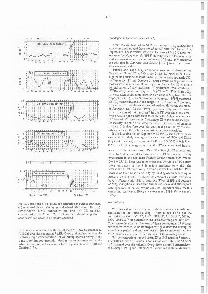
0 E C:
20
.. '-o. 40
E ëi 20 E
N N N N N - - - - - N
:!. 0 4-.,-;....;....;_...;,.~.;....;......:,;...-,..;....;....;....;....;....;.,;..+-;-+-,;....;....;..>;<~....;....,-,;-+-r""i-i-+
1 2
E 8 0
ê 4
--NNNNN - - - - - N
0 ..;....;.....;.........,....;,...,;.....;........,....,....,,_..,._......,...,._.,_..........,...,....,,........_,.........,....--,.......,.....--r->t-+-
'7 E l.l
- - N N N N N
IP!C! Oc.
Seplember 1991
p
- - .,... N
C Oc.
- .,... .,... - - N
October 1991
Fig. 3. Variations of (a) DMS concentration in surface seawater, (b) estimated piston velocity, (c) calculated OMS sea-air flux, (d) atmospheric DMS concentration, and (e) CN number concentration. P. C and Oc. indicate periods when polluted, continental and oceanic air masses occurred.
Tiùs value is consistent with the estimate of 1 day by Baies et al.
(1992b] over the equatorial P~cific Ocean, taking into account the probably high concentrations of oxidizing species owing to the a!most continuous insolation during our experiment and to the advection of polluted air masses for 5 days (September 17-18 and Octobcr 5-7 ).
106
Atmospheric Concen1ra1ions of S02
- Over the 27 days when SO2 was sampled, its atmospheric concentrations ranged from .<0.15 to 4.7 nmol m·3 (mean, J.5; Figure 4a). These values are close to those of 0.5-3.9 nmol m·J observed by Nguyen et al. (1983] in May 1974 in the same area and are consistent with the annual mean of 2 nmol m·3 calculated for this area by Langner and Rhode (1991] from their three-dimensionnal mode!.
Particularly high SO2 concentrations were observed on September 18 and 22 and October 5 (4.6-4.7 nmol m·3). These high values must be at least partially due to anthropogenic SO2 on September 18 and October 5, since advection of polluted air masses was indicated on these days. For September 22, we have no indication of any transport of pollutants from continents (222Rn daily mean activity = 1.3 pCi m· 3). This high sp,,_ concentration could corne from entrainment of SO2 from the free troposphere (Ff), since Ockelman and Georgii (1989] measured six SO2 concentrations in the range 1.3-19.7 nmol m·3 (median, 5.3) in the FT over the west coast of Africa. However, the mode] of langner and Rhode (1991] predicts SO2 annual mean concentrations of 1-2 nmol m·3 in the FT over the study area, which would not be sufficient to explain the SO2 concentration of 4.6 nmol m·3 observed on September 22 in the boundary layer. On that day, the ship often described circ!es to reach hydrographie stations. It is therefore possible that local pollution by the ship exhaust affected the SO2 concentration on those occasions.
If the data obtained on September 18 and 22 and October 5 are exc!uded, the daily average concentrations of SO2 and OMS (Figure 4 a and 4b) are corre!ated (SO2 = 0.3 OMS + 0.2; R = 0.73, P < 0.001), suggesting that the SO2 encountered in this
area is mainly derived from OMS. The SO2 /DMS ratio is very close to that observed by Bandy et al. (1992] during a 7-day experiment in the northeast Pacifie Ocean (mean SO2 /mean OMS = 25(78). Ooes this ratio mean that the -yield of Süi from OMS oxidation is low? It might indicate only that the atmospheric lifetime of SQi is much shorter than that for OMS, because of the oxidation of SO2 by OH/O2 which according to Atkinson et al. (1989]. is almost as efficient as DMS oxidation by OH (Hynes et al., 1986; Hynes and Wine, 1989], and because of SO2 absorption in seawater and/or sea spray and subsequent hcterogeneous oxidation, which are a!so important sinks for this compound [lelieveld, 1990; Sievering et al., 1991; Putaud et al., 1992].
Aerosol Ions
We focused our attention on submicrometer aerosols and analyzed the 26 sampled final fi!ters (stage 6) to get the concentrations of Na+, K+, Ca2+, HCOO-, CH3COO·, MSA, NO3·, and SO/· in particles in the diameter range of <0.6 µm. To estimate the size distributions of these compounds, 17 6-stage series were chosen to be homogeneously distributed during the experiment period and analysed for ail these compounds except MSA, which was analyzed in only nine of these 6-stage series.
Na+ concentrations ranged from 23 to 343 nmol m·3 (mean, 117; data not shown). which is consistent with values of 70 nmol m·3 obtaincd over the Atlantic Ocean from a ship (Bürgermeister and Georgii, 1991) and 130nmol m·3 measurcd at Bermuda Island
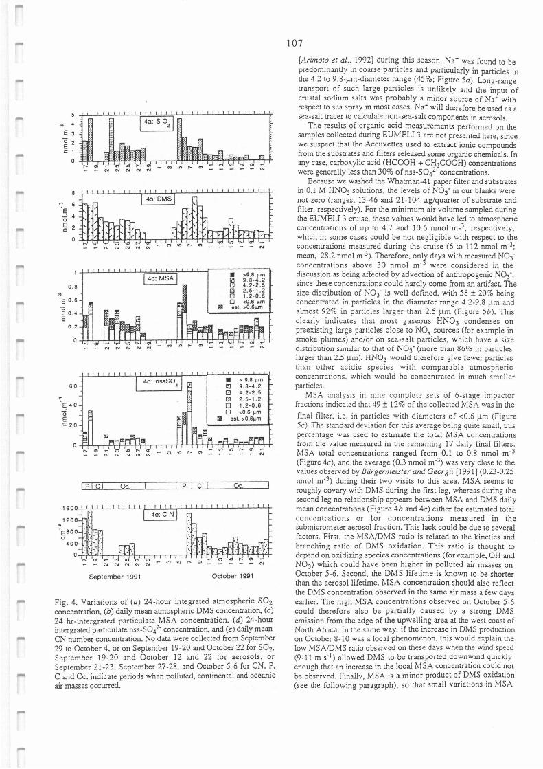
E 3
ëi 2 E C: 1
0
8
.... 6 E ëi 4
E 2 C:
0
60
.... E 40
ëi E c: 2 0
1600
1200
EBOO u
400
0
- - N N
..... "' - M Il') ,-... Q'I
N N N N N
1 P! C! Oc
"' - - N N
September 1991
• > 9.8 µm ~ 9. 8-4 . 2 G 4.2-2 . 5 l:J 2.5-1.2 0 1.2-0. 6 D <0.6 µm
Ill esl. ,0.6µm
- M \I') ,-... en
p ç Oc
- M ., - - - - - N
October 1991
Fig. 4. Variations of (a) 24-hour integrated atmospheric SO2 concentration, (b) daily mean atmospheric DMS concentration, (c) 24 hr-intergrated particulate MSA concentration, (d) 24-hour intcrgrated. particulate nss-SOl· concentration, and (e) daily mean CN number concentration. No data were collected from Septembcr 29 to October 4, or on September 19-20 and October 22 for SO2, September 19-20 and October 12 and 22 for aerosols, or September 21-23, September 27-28, and October 5-6 for CN. P. C and Oc. indicate periods when polluted, continental and oceanic air masses occurred.
107
[Arimoto et al., 1992] during this season. Na+ was found to be predominanùy in coarse partic!es and particularly in partic!es in the 4.2 to 9.8-µm-diameter range (45%; Figure Sa). Long-range transport of such large particles is unlikely and the input of crustal sodium salts was probably a miner source of Na+ with respect to sca spray in most cases . Na+ will therefore be used as a sea-salt tracer to calculate non-sea-salt componems in aerosols.
· The results of organic acid measurements performed on the samples collected during EUMELI 3 are net presented here, since we suspect that the Accuvettes used to extract ionic compounds from the substrates and filters released some organic chemicals. In any case, carboxylic acid (HCOOH + CH3COOH) concentrations were generally less than 30% of nss-So/- concentrations.
Because we washed the Whatman-41 paper filter and substrates in 0.1 M HNO3 solutions, the !evels of NO3· in our blanks were net zero (ranges, 13-46 and 21-104 µg/quarter of substrate and filter, respectively). For the minimum air volume sampled during the EUMELI 3 cruise, these values would have led to atmospheric concentrations of up to 4.7 and 10.6 nmol m-3, respectively, which in some cases could be net negligible with respect to the concentrations measured during the cruise (6 to 112 nmol m·3; mean, 28.2 nmol m·3). Therefore, only days with measured NO3· concentrations above 30 nmol m·3 were considered in the discussion as being affected by advection of anthropogenic NO3·, since these concentrations could hardly corne from an artifact. The size distribution of NO3· is well defined, with 58 ± 20% being concentrated in partic!es in the diameter range 4.2-9.8 µm and almost 92% in particles larger than 2.5 µm (Figure Sb). This clearly indicates that most gaseous HNO3 condenses on preexisting large partic!es close to NO, sources (for example in smoke plumes) and/or on sea-salt particles, which have a size distribution similar to that of NO3· (more than 86% in particles larger than 2.5 µm). HNO3 would therefore give fewer particles than other acidic species with comparable atmospheric concentrations, which would be concentrated in much smaller partic!es .
MSA analysi s in nine complete sets of 6-stage impacter fractions indicatcd that 49 ± 12% of the col!ected MSA was in the
final filter, i.e. in particles with diameters of <0.6 µm (Figure 5c). The standard deviation for this average being quite small, this percentage was used to estimate the total MSA concentrations from the value measured in the remaining 17 daily final filters. MSA total concentrations ranged from 0.1 to 0.8 nmol m·3
(Figure 4c), and the average (0.3 nmol m·3) was very close to the values observed by Bürgermeister and Georgii [1991] (0.23-0.25 nmol m·3) during their two visits to this area. MSA seems to roughly covary with DMS during the first leg, whereas during the second leg no relation.ship appears between MSA and DMS daily mean concentrations (Figure 4b and 4c) either for estimated total concentrations or for concentrations measured in the submicrometer aerosol fraction. This Jack could be due to several-factors . First, the MSA/DMS ratio is related to the kinetics and branching ratio of DMS oxidation. This ratio is thought to depend on oxidizing species concentrations (for example, OH and NO 3) which could have been higher in polluted air masses on October 5-6. Second, the DMS lifetime is known to be shorter than the aerosol lifetime. MSA concentration should also reflect the OMS concentration observed in the same air mass a few days earlier. The high MSA concentrations observed on Octobcr 5-6 could therefore aise be partially caused by a strong DMS emission from the edge of the upwelling area at the west coast of North Africa. In the same way, if the increasc in OMS production on October 8-10 was a local phenomenon, this would explain the low MSA/DMS ratio observed on these days when the wind specd (9-11 m s·1) allowed OMS to be transported downwind quickly enough that an increase in the local MSA concentration could net be observed. Finallv, MSA is a miner product of OMS oxidaùon (see the following paragraph), so that small variations in MSA
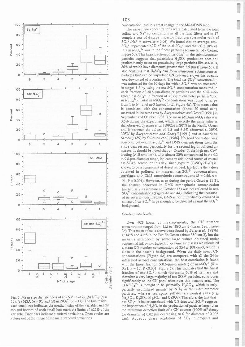
100+-----=~----'------'----'-----'----t-
r sa :~· 1
C: a,
~ a, a..
80
60
6 5 4 3 2
100--!,..--..i..-----'----'-----'---_,__---i-
C: a,
~ a,
80
60
a.. 40
20
Sb: No3
•
6
0
5 4 3 2
100-+------'---~---~--~---.----...-Sc: MSA
80
; 60 $ ~ a, a.. 40
0 0 8
20
= 8 9~ 0 4---~--~--'"----.--g---.--~--.--' _:::: __ ,-t-
6 5 4 3 2
1 00 +---'-----'----'-----'--.========;t-1 sd: nss-so/· 1
80
c: 60 a,
~ a, a.. 40 $
6 4 ~ 3 N
0 ~ :.. a,
N° of stage ::, -(.) Ë
"' 'o
Fig. 5. Me:m size distributions of (a) Na• (n=l 7), (b) NO3· (n = 17), (c) MSA (n = 9), and (d) nssSOi· (n = 17). The line inside each small box. indicates the median value of the variable, and the top and bottom of each small box. mark the limits of ±25% of the variable. Errer bars indicate standard deviations. Open circles arc values out of the range of means ± standard deviations.
108 concentration lead to a great change in the MSA/OMS ratio.
The nss-sulfate concentrations were calculated from the total sulfate and Na• concencrations in ail the final filters and in 17 comtcte sets of 6-scage impacter fractions (the molar ratio of SO4 ·;Na• in seawacer = 0.06). We found that on average, nss-soi· represented 62% of the cotai soi· and that 60 ± 18% of this nss-SO/· was in the finest particles (diameter of <0.6µm; Figure 5d). This large fraction of nss-SOi· in the submicrometer particles suggests that particulate-H2SO4 production does not predominantly occur on preexisting large particles like sea-salts, 86% of which have diameters greater than 2.5 µm (Figure 5a). It also confirms that H2SO4 can form numerous submicrometer particles that can be important CN precursors over this oceanic area downwind of a continent. The total nss-SOi· concentration was estimated for the 10 days for which SOi· was not measured in stages 1-5 by using the nss-SOi· concentration measured in each fraction of <0.6-µm-diameter particles and the 60% ratio (mean nss-SOi· in fraction of <0.6-µm-diameter particles/total nss-SO/·). Total nss-SO42· concentration was found ta range from 1 ta 64 nmol m-3 (mean, 14.2; Figure 4d). This mean value is consistent with the concentration (about 20 nmol m·3) measured in the same area by Bürgermeister and Georgii (1991) in September and October 1988. The mean MSNnss-SO4 ratio was 3.5% during the ex.periment, which is ex.actly the same value as that observed by Baies et al. [1992b] at 20°N in the Pacifie Ocean and is between the values of 1.5 and 6.5% observed ac 20°N, 30°W by Bürgermeister and Georgii (1991) and at American Samoa (14°S) by Saltzman et al. (1986). No good correlation was observed between nss-SOi· and OMS concentrations from the entire data set and particularly for the second leg in polluted air masses. It should be noted that on October 7, the high nss-Ca2+
loading (> 10 nmol m·3), with almost 80% concentrated in the 4.2 to 9.8-µm-diamecer range, indicates an additional source of crustal nss-SO42- aerosol on this day, since gypsum (CaSO4·2H2O) is known ta be a component of desert aerosol. Ex.cluding the values obtained in polluted air masses, nss-SOi· concentrations
_c_cmel~d with_OMS atrn9spheric _concentrations_(R = 0.66 .. n = 21, P < 0.001). However, even during the period October 11-21, the feature observed in OMS atrnospheric concentration (parcicularly its increase on October 15) was not reflected in nss-SOi· concentrations (Figure 4b and 4d), indicating that because of its several-hour lifetirne, OMS is not irnmediately ox.idized in a mass of nss-so/· large enough lO be detected against the soi· background.
Condensaiion Nucfei
Over 402 hours of measurements, the CN number concentration ranged from 155 to 1890 cm-3 (mean, 586; Figure 3e). Tiûs mean value is above those found by Bates et al. [1987b) at 14°S and 41 °Sin the Pacifie Ocean (about 380 cm-3), but the mean is influenced by some large values obtained under continental influence. Indeed. in oceanic air masses we calculated a mean CN number concentration of 354 ± 108 cm-3, which is close to the oceanic background. When the daily mean CN concentrations (Figure 4e) are compared with all the 24-hr integrated aerosol concentrations, the best correlation is found with the finest fraction (<0.6-µm-diarneter) of nss-SOi· (R = 0.91, n = 17, P <0.001; Figure 6). This indicates that the finest fraction of nss-SO/·, which represents 60% of its mass and therefore a very large majority of nss-SO/· particles, contributes significantly to the CN population over this oceanic area. The nss-SOi· is thought ta be prirnarily H2S 04, which is only partially neutralized mainly by NH3 in the submicrometer particles , whereas sea spray sulfates are neutral salts (c.g. Na2SO4, K2SO4, MgSO4, and CaSO4). Therefore, the fact that nss-SOi· is better correlated with CN than total SOi· suggests the importance of H2SO4 in the production of particles larger than the minimum dccection limit of a CN counter (100% efficiency for diameter of 0.02 µm decreasing to O for diameter of 0.005 µm ). Aqueous phase oxidation of SO2 in droplets and
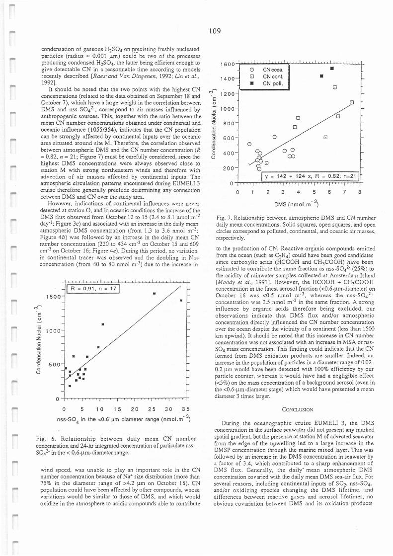
condensation of gaseous H2SO4 on P,r_existing freshly nucleated panic!es (radius == 0.001 µm) could be two of the proccsses producing condensed H2SO4, the latter being efficient enough to give detectable CN in a reasonnable time according to models recently described [Raes,-and Van Dingenen, 1992; lin et al.,
1992]. Il should be noted that the two points with the highest CN
concentrations (related to the data obtained on September 18 and October 7), which have a large weight in the correlation between DMS and nss-SOi·. correspond to air masses influenced by anthropogenic sources. This, together with the ratio between the mean CN number concentrations obtained under continental and oceanic influence (1055/354). indicates that the CN population can be strongly affected by continental inputs over the oceanic area situated around site M. Therefore. the correlation observed between atrnospheric DMS and the CN number concentration (R
= 0.82, n = 21; Figure 7) must be carefully considered, since the highest DMS concentrations were always observed close to station M with strong northeastem winds and therefore with advection of air masses affected by continental inputs. The atmospheric circulation patterns encountered during EUMELI 3 croise therefore generally preclude determining any connection between OMS and CN over the study are.a.
However, indications of continental influences were never detected ac station 0, and in oceanic conditions the increase of the OMS flux observed from October 12 to 15 (2.4 to 8.1 µmol m·2
day· 1; Figure 3c) and associated with an increase in the daily mean atmospheric DMS concentration (from 1.3 to 3.6 nmol m· 3;
Figure 4b) was followed by an incrcasc in the daily mean CN number concentration (220 to 434 cm·3 on October 15 and 609 cm·3 on October 16; Figure 4e). Ouring this period, no variation in continental tracer was observed and the doubling in Na+ concentration (from 40 to 80 nmol m·3) due to the increase in
R = 0 .91, n 171 • 1500 • ,.,-
E 0
• ,ii 1000 0
::, z C 0 • ·;:,
~ • • C
~ 500 8 • • • •••
0
0 5 1 0 1 5 20 25 30 35
nss-S04
in the <0.S-µm diameter range (nmol.m.3)
Fig. 6. Relationship between daily mean CN number concentration and 24-hr integrated concentration of particulate nss-SO/· in the< 0.6-µm-diameter range.
wind spced. was unable to play an important role in the CN number concentration becausc of Na+ size distribution (more than 75% in the diarneter range of >4.2 µm on October 16). CN population could have been affccted by other compounds, whose variations would be similar to chose of OMS. and which would oxidize in the atmosphere to acidic compounds able to contribute
109
1600 '1 Li..JJ..LL -0 CNoœa. •
1400 0 CN cont. • • CN poli . 0
C"l-1200
E (J
·a; u ::J z C 0
:::,
~ C QJ
~ 0
(.)
1000
800
600 0
400
200
0
0
0 0
0
0 0
0 0 œ
y = 142 + 124 X, A = 0.82, n=21
2 3 4 5
• 3 OMS (nmol.m )
6 7 8
Fig. 7. Relationship between atmospheric DMS and CN number daily mean concentrations. Solid squares, open squares, and open circles correspond to polluted. continental, and oceanic air masses, respectively.
to the production of CN. Reactive org~ic compounds emitted from the ocean (such as C2H4) could have been good candidates since carboxylic acids (HCOOH and CH3COOH) have been estirnated to contribute the sarne fraction as nss-SOi· (25%) to the acidiry of rainwatcr sarnples collected at Amsterdam Island [Moody et al., 1991]. However, the HCOOH + CH3COOH concentration in the finest aerosol fraction (<0.6-µm-diameter) on October 16 was <0.5 nmol m· 3, whereas the nss-SO4
2· concentration was 2.5 nmol m·3 in the same fraction. A strong influence by organic acids therefore being excluded, our observations indicate chat DMS flux and/or atmospheric concentration directly influenced the CN number concentration over the ocean despite the vicinity of a continent (Jess chan 1500 lem upwind). It should be noted that this increase in CN number concentration was not associated with an increase in MSA or nss-SO4 mass concentration. This finding could indicate that the CN formed from OMS oxidation products are smaller. Indeed, an increase in the population of particles in a diarneter range of 0.02-0.2 µm would have been detected with 100% efficiency by our particle counter, whereas it would have had a ncgligible effect (<5%) on the mass concentration of a background acrosol (evcn in the <0.6-µm-diameter stage) which would have presented a mean diameter 3 tirnes larger.
CONO..USION
Ouring the oceanographic cruise EUMELI 3, the OMS concentration in the surface scawater did not present any marked spatial gradient, but the prescnce at station M of advected seawatcr from the edge of the upwelling led to a large increase in the OMSP concentration through the marine mixed layer. This was followed by an incrcase in the DMS concentration in seawater by a factor of 3.4. which contributed to a sharp enhancement of OMS flux. Gencrally, the daily· mcan atmospheric OMS concentration covaried with the dai1y mean OMS sca-air flux. For several reasons, including continental inputs of SO2, nss-SO4, and/or oxidizing species changing the DMS lifetime, and diffcrences between reactive gases and aerosol lifetimcs. no obvious covariation betwcen OMS and its oxidation products
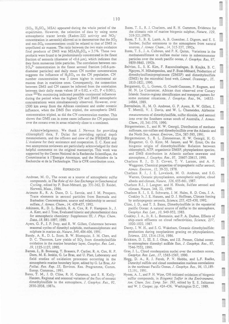
110
(SO2 , H2SO4, MSA) appeared·during the whole period of the experiment. However, the selection of data by using some atmospheric tracer !evels (Radon-222 activity and NO3 · concentration in aerosols) al!owed us to demonstrate that the SO2 and nss-SO4 concentrations could be related to that of DMS in unpolluted air masses. The ratio between the two main oxidation final products of DMS was MSA/H2SO4 = 3.5%. These two products were found to be predominantly concentrated in the finest fraction of aerosols (diameter of <0.6 µm), which indicates that they form numerous little particles. The correlation between nss-S Oi· concentration in the finest aerosol fraction ( <0.6-µm-diameter particles) and daily mean CN number concentration suggests the influence of H2SO 4 on the CN population. CN number concentration was 3 times higher in continental air masses than in maritime ones. Consequently, the connection between OMS and CN cannot be inferred from the correlation between their daily mean values (R = 0.82. n =21, P < 0.001). since 222Rn monitoring indicated possible continental influences during the period when the highest CN and OMS atmospheric concentrations were simultaneously observed. However, over 1500 km away from the African continent and under oceanic influence. when the DMS flux tripled, the atmospheric OMS concentration tripled, as did the CN concentration number. This shows that OMS can in some cases influence the CN population over the oceans even in areas relatively close to a continent.
Acknowledgments . We thank J. Neveux for providing chlorophyll data, F. Dulac for providing optical depth measurements, and the officers and crew of the IFREMER ship L'Atalante for their assistance and cooperation. E. C. Kent and rwo anonymous reviewers are particularly acknowledged for their helpful comments on the original manuscript. This work was supported by the Centre National de la Recherche Scientifique, the Commissariat à !'Energie Atomique, and the Ministère de la Recherche et de la Technologie. This is CFR contribution xxxx.
REFERENCES
Andreae, M. O., The ocean as a source of atmospheric sulfur compounds, in The Role of Air-Sea &change in Geochemical
Cycling, edited by P. Buat-Ménard, pp. 331-362. D. Reidel, Horwell, Mass., 1986.
Arimoto R., R. A. Duce, D. L. Savoie, and J. M. Prospero , Trace e!ements in aerosol particles from Bermuda and Barbados: Concentrations. source and relationship to aerosol sulfate, J. Atmos. Chem., 14, 439-457, 1992.
Atkinson, R., D. L. Baulch. R. A. Cox, R. F. Hampson Jr., J. A. Kerr. and J. Troe, Eva!uated kinetic and photochemical data for atrnospheric chemistry: Supplement III, J. Phys. Chem.
Data, 18, 881-1097, 1989. Ayers, G. P .• J. P. Ivey, and R. W. Gillet[, Coherence between
seasona1 cycles of dimethyl sulphide, methanesulphonate and sulphate in marine air. Nature, 349, 404-406, 1991.
Bandy, A. R .. D. L. Scott, B. W. Blomquist, S. M. Chen, and D. C. Thornton, Low yields of SO2 from dimethylsulfide oxidation in the marine boundary layer, Geophys. Res. Lett ., 19, 1125-1127, 1992.
Barnes, I., B. Bonsang, T. Brauers, P. Carlier, R. A. Cox, H. P. Dom, M. E. Jenkin, G. Le Bras, and U. Platt, Laboratory and field studies of oxidation processes occurring in the atmospheric marine boundary layer, edited by G. Le Bras, Air PolluJ. Res. Rep. 35, Environ. Res. Programme, Comm. Europ. Commun .• 1991.
Bates, T. M .• J. D. Cline, R. H. Gammon, and S. R. Kelly-Hansen, Regiona1 and seasona1 variation of the flux of oceanic dimethylsulfide to the atmosphere, J. Geophys. Res., 92 , 2930-2938, 1987a.
Bates, T. S .. R. J. Charlson. and R. H. Gammon, Evidence for the climatic role of marine biogenic sulphur, Nature , 329,
319-321.1987b. Bates, T. S .. B. K. Lamb. A. B. Guenther, J. Oignon, and E. S.
Stoiber, Sulfur emissions co the atmosphere from natural sources. J. Atmos. Chem ., 14, 315-337, 1992a.
Bates. T . S., J. A. Calhoun, and P. K. Quinn, Variations in the methanesulfonate to sulfate molar ratio in submicrometer particles over the south pacifie ocean, J. Geophys. Res, 97, 9859-9865, 1992b.
Belviso, S., S. K. Kim, F. Rassoulzadegan, B. Krajka, B. C. Nguyen, N. Mihalopoulos, and P. Buat-Ménard, Production of dimethylsulfoniopropionate (DMSP) and dimethylsulfide (OMS) by the microbial food web, Limnol. Oceanogr., 35, 1810-1821. 1990.
Bergametti, G., L. Gomes, G. Coudé-Gaussen, P. Rognon, and M. N. Le Costumier, African dust observed over Canary Islands: Source-regions identification and transport pattern for some summer situations, J. Geophys. Res., 94, 14855-14864, 1989.
Berresheim, H., M. O. Andreae, G. P. Ayers, R. W. Gillet[, J. T. Merrill. V. J. Davis. and W. L. Chameides. Airbome
measurements of dimethylsulfide, sulfur dioxide, and aerosol ions over the Southern ocean south of Australia, J. Atmos. Chem., JO, 341-370, 1990.
Bürgerrneister, S., and H. W. Georgii. Distribution of methane sulfonate, nss-sulfate and dimethylsulfide over the Aùantic and the North Sea, Atmos. Environ., 25A. 587-595, 1991.
Bürgermeister, S., R. L. Zimmerrnan, H. W. Georgii, H. G. Bingemer, G. O. Kirst. M. Jansen, and W. Ernst, On the biogenic origin of dimethylsulfide: Relation between chlorophyll, ATP. organismic DMSP, phytoplankton species, and OMS distribution in Atlantic surface seawater and atmosphere, J. Geophys. Res., 95, 20607-20615. 1990.
Charlson R. J., D. S. Covert. T . V. Larson, and A. P. Waggoner. Chemical properties of tropospheric sulfur aerosol, Atmos. Environ., 12, 39-53, 1978.
Charlson R. J., J. E. Lovelock, M. O. Andreae, and S.G. Warren. Oceanic phytoplankton, atmospheric sulphur, cloud albedo and climate, Nature , 326, 655-661, 1987.
Charlson R.J .• J. Langner, and H. Rhode, Sulfate aerosol and climate, Nature, 348, 22, 1990.
Char.lson R. J .• S. E. Schwartz, J. M. Hales, R. D. Cess, J. A. Coakley Jr. J. E. Hansen, and D. J. Hoffman, Climate forcing by anthropogenic aerosols, Science, 255, 423-430, 1992.
Cline, J. D., and T. S. Bates, Dimethylsulfide in the equatorial pacifie Ocean: A natural source of sulfur to the atmosphere, Geophys. Res. Lect., JO, 949-952. 1983.
Coakley. J. A., Jr, R. L. Bernstein, and P. A. Durkee, Effects of ship-stack effluents on cloud reflectivities, Science, 237, 1020-1022, 1987. .
Dacey, J. W. H .• and S. G. Wakeham, Oceanic dimethylsulfide: production during zooplankton grazing on phytoplankton, Science, 233, 1314-1316. 1986.
Erickson, D. J., ID. S. J. Ghan, and J.E. Penner, Global ocean-to-atrnosphere dimethyl sulfide flux, J. Geophys. Res., 95, 7546-7552, 1990.
Gras, J. L., Cloud condensation nuclei over the southem ocean, Geophys. Res. Lett., 17, 1565-1567, 1990.
Hegg. D. A .• R. J. Ferek, P. V. Hobbs, and L.F. Radke, Dimethyl sulfide and cloud condensation nucleus correlations in the northeast Pacifie Ocean, J. Geophys. Res., 96, 13,189-13,191. 1991.
Hynes, A. J.. and P. H. Wine, OH-initiated oxidation of biogenic sulfur compounds. in Biogenic Sulfur in the Environment,
Am. Chem . Soc. Symp . Ser . 393, edited by E. S. Saltzman and W. J. Cooper, pp. 424-436, Washington D.C., 1989.
111
Hynes, .-\. J., P. H. Wine, and O. H. Semmes, Kinetics and mechanisms of OH reactions wir.h organic sulfides, J. Phys. Chem., 90, 4148-4156, 1986.
Keller, M. O., W. K. Bellows, and R. R. L. Guillard. Dirnethylsulfide production in marine phytoplankton, in Biogenic Su/fur in the EnvironmenJ, Am. Chem. Soc. Symp. Ser . 393, edited by E. S. Sa!tzman and W. J. Cooper, pp. 167-182, Washington D.C., 1989.
Kiene, R. P .• and T. S. Bates. Biologica! removal of dirnethylsulfide from seawater, Na1ure, 345, 6277-6279, 1990.
Langner. J., and H. Rhode, A global three-dimensional mode! of the tropospheric sulfur cycle, J. Almos. Chem., 13, 225-263, 1991.
Legrand. M. R., R. J. Delmas , and R.J. Charlson, Climate forcing implication from Vostok ice-core sulphate data. Na1ure, 334, 418-420, 1988.
Leiatch, W. R., G . A. Isaac, J. W. Strapp. C. M. Banic, and H.A . Wiebe, The re!ationship between c!oud droplet number concentrations and anthropogenic pollution: Observations and climatic implications, J. Geophys. Res., 97, 2453-2474,1992.
Lelieveld, J., The role of c!ouds in tropospheric photochemistry, Ph. D. thesis, Univ. of Utrecht, Utrecht, Netherlands, 1990.
Lin, X .• W. L. Chameidcs, C. S. Kiang, A. W. Stelon, and H. Berresheim, A mode! study of the formation of cloud condensation nuc!ei in remote marine areas, J. Ceophys. Res. ,
92, 18161- 18171, 1991. Liss. P. S ., and L. Mer!ivat, Air-sea gas exchange rates:
Introduction and synthesis. in The Roie of Air-Sea E:cchange in Geochemical Cycling, edited by P. Buat-Ménard, pp. 113-128, D. Reidel, Horwell, Mass., 1986.
Luria. M., C. C. Van Valin, J. N. Galloway, W. C. Keene, O. L. Wellman, H . Sievering, and J . F. Boatman, The relationship between dirnethylsufide and particulate sulfate in the mid-Atlantic ocean atmosphcre, Almos. Environ., 23 , 139-147, 1989.
Mihalopoulos, N ., B. C. Nguyen, J. P. Putaud, and S . Belvis_o, The oceanic source of carbonyl sulfide (COS), Almos. Env1r.,
26A, 1383-1394, 1992. Moodv, J. L., A. A. P. Pszenny, A. Gaudry, W. C. Keene, J. N.
Gal!oway, and G. Polian, Precipitation composition and its variability in the Southern Indian Ocean: Amsterdam Island, 1980-1987, J. Ceophys. Res., 96, 20769-20786, 1991.
Nguyen, B . C., B. Bonsang, and G. Lambert, The atmospheric concentration of sulfur dioxide and sulfate aerosol over antarctic, subantarctic areas and ocean, Te/lus, 26, 241-247, 1974.
Nguyen B. C., B. Bonsang, and A. Gaudry, The role of the ocean in the global atmospheric sulfur cycle, J. Ceophys. Res., 88,
10903-10914, 1983. Nguyen, B. C., S . Be!viso, N. Mihalopo_ulos, J. ~ostan, and P.
Nival, Dimethylsulfide production durmg natural phytoplanktonic bloorns, Marine Chem., 24, 133-141, 1988 .
Nguyen, B . C., N . Mihalopoulos, and S. Belviso, Seasonal variation of atmospheric dimethyl sulfide at Amsterdam Island in the southern Indian Ocean, J. Almos. Chem., 11, 123-143, 1990.
Nguyen, B. C., N . Mihalopoulos, J. P. Putaud, A . Gaudry, L. Gallet, W. C. Keene, and J. N. Galloway, Covariations in oceanic dimer.hylsulfide, its oxidation products and rain acidity at Amsterdam Island in the southern Indian Ocean, J. Atmos.
Chem., 15, 39-53, 1992. Ockelman, G. E. F., and H. W . Georgii, Grossraumige
Veneilung des atmospharischen Schwcfcldioxids in der frcien Troposphare, Meteoro/. Ruruisch., 41, 136-146, 1989.
Polian. G .• G. Lambert, B. Ardouin. and A. Jégou, Long range transport of continental radon in subantarctic · areas, Te/lus, 38B, 178-189, 1986.
Putaud. J. P., N. MihaJopoulos , B. C. Nguyen, J. M. Campin, and S. Belviso, Seasonal variations of atmospheric sulfur dioxide and dirnethylsulfide concentrations at Amsterdam Island in r.he southem Indian Ocean, J. Almos. Chem ., 15, 117-131, 1992.
Radke, L. F., J. A. Coakley, Jr., and M. D. King, Direct and remote sensing observation of the effect of ships on c!ouds, Science, 246, 1146-1149, 1989.
Raes, F .• and R. Van Dingenen, Simulations of condensation and cloud condensation nuclei from biogenic S02 in the remote marine boundary layer, J. Ceophys. Res., 97, 12901-12912, 1992.
Saltzman, E. S., D. L. Savoie, J. M. Prospero, and R. G. Zika, Methane sulfonic acid and non-sea-salt sulfate in Pacifie air: Regional and seasonal variations, J. Atmos. Chem., 4, 227-240, 1986. .
Sievering, H., J. F. Boatman, J. N. GaJloway, W . C. Keene, Y. Kim, M . Luria, and J. Ray, Heterogeneous sulfur conversion in sea-salt aerosol particles: The role of aerosol water content and size distribuuon, Atmos. Environ., 25A , 1479-1487, 1991.
Twomey, S., The composition of cloud nuclei , J. Atmos. Sei., 28, 377-381, 1971.
Watts, S. F., R. Yaaqub, and T. Davies, Comments on ''The use of Whatman 41 filter papers for high volume aerosol sampling" by Lodge, [1986), Almos. Environ., 21, 2731-2732, 1987.
Wigley, T. M. L., Possible climatic change due ro S02-derived cloud condensation nuclei, Nalure, 339, 365-367, 1989.
Yin F., O. Grosjean, and J. H. Seinfeld, Photooxidation of dimethylsulfide and dimethyldisulfide, I. Mechanism development, J. Atmos. Chem., 11, 309-344, 1990.
S. Belviso, N. · Mihalopoulos, B.C. Nguyen, and J.P,. Putaud, Centre des Faibles Radioactivités, Laboratoire mixte CNRS -CEA, Ave. de la Terrasse. F-91198 Gif-sur-Yvette Cedex, France.
(Reccived December 1. 1992; revised March 18, 1993; accepted March 23, 1993)

113
Conclusion
Les résultats obtenus lors de cette expérience montrent que la population de CN au-dessus
de l'océan Atlantique tropical nord est généralement affectée par le transport de masses d'air
continentales dans lesquelles des traces de pollution sont parfois détectées. Les
concentrations et la granulométrie des aérosols de composés soufrés indique que l'acide
sulfurique entre pour une part importante dans la composition des aérosols submicroniques.
La corrélation entre le nombre de CN et la concentration de sulfates en excès dans ces
aérosols de diamètre inférieur à 0.6 µm montre d'ailleurs que l'acide sulfurique est une
composante majeure des noyaux de condensation.
La comparaison entre concentration atmosphérique de OMS et noyaux de condensation, qui
était le but de cette expérience, pourrait sembler édifiante puisqu'une corrélation
significative est observée entre ces deux paramètres. Cependant, les plus fortes
concentrations de OMS, enregistrées au-dessus des régions de forte productivité situées près
de la côte africaine, étaient observées alors que les masses d'air échantillonnées étaient
affectées par des introductions de particules provenant de l'érosion éolienne ou de sources de
pollution, associées à de fortes activités en Radon et à des concentrations élevées de nitrates
ou de calcium. La corrélation entre OMS et CN mise en évidence ne permet donc pas de
conclure à une contribution significative des processus d'oxydation du OMS à la formation de
noyaux d'Aïtken.
Cependant, malgré la quasi-persistance des alizés soufflant du nord-est, la présence de
masses d'air affectées par des introductions continentales n'a jamais été détectée à plus de
1500 km à l'ouest des côtes africaines. Ces observations effectuées sur quelques semaines ne
peuvent évidemment être généralisées, et n'interdisent de toute façon pas que des transports
de composés d'origine continentale aient lieu à plus haute altitude. Néanmoins, dans les
conditions océaniques rencontrées à cette distance du continent, un triplement du flux océan-
atmosphère de OMS, accompagné par un triplement de sa concentration atmosphérique, fut
suivi par un triplement de la concentration de CN. L'émission de OMS peut donc avoir une
114
influence quasi-immédiate sur la population de noyaux d'Aïtken, comme il l'a été observé par
Andreae et al. (1993) dans l'hémisphère sud. Les processus physico-chimiques de
transformation du OMS pourraient donc contrôler la population de noyaux de condensation
au-dessus des océans, et ceci même sur une très large fraction de l'hémisphère nord.
Comment expliquer ce résultat, vu l'énorme supériorité du flux de S02 anthropogénique par
rapport au flux de OMS estimé pour l'hémisphère nord ? Il faut sans aucun doute considérer
l'hypothèse de Charlson (1992) qui estime que seuls 5% des molécules de S02 émises par
les sources anthropogéniques participent à la formation de nouvelles particules, les autres
étant oxydées en phase hétérogène, soit près de la source de pollution (dans le panache de
fumée), soit dans les gouttelettes des nuages, c'est-à-dire dans des particules préexistantes.
A l'inverse, le OMS, étant beaucoup moins soluble dans l'eau, pourrait aussi donner
directement des acides en phase gazeuse, qui par nucléation bimoléculaire avec la vapeur
d'eau forment en atmosphère propre des milliers de nouvelles particules succeptibles de
croître pour donner des noyaux d'Aïtken.

115

-,...
117
Etudié depuis plus de vingt ans, le cycle biogéochimique du soufre a d'abord suscité
l'intérêt pour l'impact que pouvait avoir la pollution de l'air par le S02 anthropogénique sur
la santé des hommes et sur l'acidification des précipitations, suspectée d'entraîner
l'accélération de la corrosion , le dépérissement des forêts et la désertification de lacs
scandinaves. Depuis une dizaine d'années, l'hypothèse d'une contribution du DMS à la
formation de noyaux de condensation (Shaw, 1983; Nguyen et al., 1983), mise en forme par
Charlson et al. (1987), a relancé l'intérêt de l'étude du cycle biogéochimique naturel du
soufre (Annexe 1) .
L'émission de DMS à la surface de l'océan est sans doute la première source naturelle de
soufre dans l'atmosphère. Cependant, les différentes estimations conduisent à des résultats
variant de 15 à 40 TgS/an, l'incertitude sur chacune des valeurs étant proche d'un facteur 2.
Ces flux de DMS sont calculés grâce à un modèle d'échange océan-atmosphère, à partir des
concentrations de DMS mesurées dans l'eau de mer et de paramétrisations du coefficient
d'échange air-mer Kw. Lors d'une expérience conduite dans l'océan Atlantique spécialement
pour étudier les flux océan-atmosphère, nous avons calculé des valeurs de flux de DMS par
cette méthode classique d'une part et en considérant la théorie de la diffusion turbulente
d'autre part. Par cette approche , le flux de DMS est obtenu à partir de mesures du gradient
de DMS dans l'atmosphère et de paramétrisations du coefficient de diffusion turbulente (K2 )
en fonction de paramètres physiques mesurés pendant la campagne. En comparant les valeurs
de flux de DMS calculés par la méthode classique avec celles données par la méthode du
gradient au même instant et au même endroit, il apparait que l'utilisation des
paramétrisations usuelles de Kw conduit à des flux de OMS en moyenne inférieurs
d'un facteur 1.3 à 2.1 aux valeurs obtenues par la méthode du gradient . Malgré les
incertitudes importantes introduites par cette nouvelle méthode, ce résultat corrobore ceux
·d'Erickson et al. (1990) qui suggèrent que l'utilisation du Kw de Liss et Merlivat (1986)
entraîne une sous estimation des flux océan-atmosphère de DMS d'un facteur 1,8. Ceci
pourrait expliquer certains déséquilibres dans le budget du soufre en milieu océanique
observés en plusieurs circonstances.
118
Les molécules de OMS émises dans l'atmosphère sont soumises aux agressions des radicaux
(OH, N03) qui initient des réactions en chaîne dont les produits principaux sont le dioxyde de
soufre, l'acide méthanesulfonique et l'acide sulfurique. La proportion des différents produits
formés dans l'atmosphère naturelle est encore mal déterminée: elle dépend des espèces
oxydantes présentes et peut-être de certains paramètres tels que la température de l'air. Les
résultats obtenus à l'île Amsterdam (Terres Australes et Antarctiques Françaises), située
par 38°S dans l'océan Indien, ont permis d'y estimer à 70 et 20% les proportions de OMS
respectivement oxydées en S02 et MSA. Cependant, cette valeur de la proportion de
OMS transformée en S02 est issue de la comparaison entre des concentrations de S02
mesurées et celles prévues par un modèle photochimique de boîte utilisant des constantes de
vitesse d'oxydation et des concentrations en radicaux oxydants OH publiées dans la littérature
qui peuvent être remises en cause. Parallèlement, la proportion de MSA formée est estimée
en comparant son dépôt humide et le flux océan-atmosphère de OMS, sur lequel l'incertitude
est importante. Ces valeurs doivent ainsi être considérées comme des limites supérieures. La
fraction de OMS restant pourrait s'oxyder en diméthylsulfoxide, diméthylsulfone, mais aussi
directement en acide sulfurique, sans passer par le S02. La contribution des acides MSA
et H2S O 4 à l'acidification des précipitations recueillies à l'île Amsterdam s'élève à
plus de 50%, ce qui suggère une participation Importante de ces produits
d'oxydation du OMS à la formation de noyaux de condensation. Il est donc important
d'établir la distribution de ces produits dans différents environnements. La phase d'oxydation
atmosphérique du DMS est en effet capitale dans l'optique de la formation des CCN: alors que
le S02, principalement oxydé en phase aqueuse, ne peut alors contribuer qu'à la croissance
de particules pré-existantes, les acides méthanesulfonique et sulfurique formés en phase
gazeuse peuvent former de nouvelles particules par nucléation homogène bimoléculaire avec
la vapeur d'eau.
Lors d'une campagne océanographique effectuée dans l'océan Atlantique tropical nord, nous
avons pu mettre en évidence une corrélation entre la concentration atmosphérique de
OMS et celle de noyaux d'Aïtken. De telles covariations à long et court terme entre les
119
flux ou concentration atmosphérique de DMS et le nombre de noyaux de condensation avaient
auparavant été mises en évidence par différentes équipes dans des zones océaniques de
l'hémisphère sud. Le cycle du soufre étant complètement perturbé par les émissions de
soufre anthropogénique dans l'hémisphère nord, on pouvait se demander dans quelles
mesures cette corrélation était significative. L'advection possible de particules d'origine
continentale pendant les périodes où les plus fortes concentrations de DMS étaient
enregistrées fut effectivement démontrée par les mesures de traceurs radioactif et ioniques.
La corrélation observée ne permit donc pas d'apporter la preuve d'un effet de l'émission de
DMS sur la population de noyaux d'Aïtken dans cette région du globe. En revanche, dans des
conditions purement océanique, une augmentation du flux et de la concentration
atmosphérique de DMS fut suivie par une augmentation de la concentration de CN.
Ceci montre que même dans l'hémisphère nord, une variation de l'émission de DMS
peut conduire à une modification presque Immédiate de la population de noyaux
d'Aïken.
L'ensemble de ce travail apporte donc des éléments sur trois étapes du cycle du DMS:
émission à la surface de l'océan, transformations chimiques et production de noyaux d'Aïtken.
Pour estimer l'impact des émissions de DMS sur l'albédo de l'atmosphère marine,
l'utilisation d'un modèle sera bien sûr indispensable . Cependant, les modèles décrivant
l'étape de production des CN et des CCN ne prévoient pas de production de ces particules dans
un temps raisonnable sous des conditions initiales conformes à celles rencontrées dans la
troposphère marine . Ceci pourrait provenir de la simplification des schémas chimiques qui
ne considèrent actuellement que le chemin réactionnel DMS->S02->H2S04, ignorant la
production de MSA et la production possible de H2S04 en phase gazeuse sans formation
·intermédiaire de S02 . La sens ibilité des résultats des modèles à l'introduction de ces
mécanismes devrait être testée.
Mais dans l'éventualité où l'influence du DMS sur l'albédo de l'atmosphère marine serait
prouvée, quelle serait son importance sur l'évolution climatique future ? On peut en effet
120
penser que cette source naturelle a toujours existé, et que son impact sur l'albédo sera
toujours constant. Pourtant, les analyses de carottes de glace prélevées en Antarctique
montrent des variations importantes de la concentration en MSA au cours des cycles
glaciaire-interglaciaire (Legrand et al., 1991 ). Ces variations pourraient refléter des
variations de la source de OMS, le MSA étant un produit spécifique de l'oxydation des
organosoufrés. Différentes expériences ont également suggéré la sensibilité de la production
de OMS à certains paramètres physiques tels que l'insolation (e.g. Bates et al., 1987). Bien
que l'effet de la température soit encore inconnu, on peut imaginer qu'un réchauffement des
océans, éventuellement entraîné par une augmentation de l'effet de serre, provoquerait une
modification de la production de OMS océanique, soit en affectant l'activité du plancton, soit
en favorisant le développement d'espèces plus ou moins productrices de OMS. Suivant l'effet
sur le flux océan-atmosphère de OMS d'un réchauffement du climat, l'influence indirecte du
OMS sur l'albédo des nuages pourrait donc produire une amplification ou une atténuation de
la modification climatique.

121

123
Andreae, M.O , Barnard, W.R. and Ammons, J.M. The biological production of dimethylsulfide in the ocean and its role in the global atmospheric sulfur budget, Ecol. Bull. , 35, 167-177, 1983.
Andreae, M.O. The ocean as a source of atmospheric sulfur compounds, in The Role of Air-Sea Exchange in Geochemical Cycling, edited by P. Buat-Ménard, D.Reidel, Hingham, Mass., 331-362, 1986 .
Andreae , M.O., Andreae, T.W. , De Mora, S .J., Elbert, W., and Schebeske, G. Biogenic sulfur, emissions, aerosol particles and cloud condensation nuclei over the Atlantic ocean, Eur. Geophys. Soc. XVIII General Assembly, Wiesbaden, 3-7 May, 1993.
Atkinson, R., Baulch, D.L., Cox, R.A., Hampson, R.F. Jr, Kerr, J.A., and Troe , J. Evaluated kinetic and photochemical data for atmospheric chemistry: supplement Ill, J. Phys. Chem. Data , 18, 881-1097, 1989 .
Ayers, G.P. , lvey, J.P. , and Gillett, R.W ., Coherence between seasonal cycles of of dimethyl sulphide, methanesulfonate and sulphate ine marine air, Nature, 349, 404-406 , 1991.
Bandy, A. R., D. L. Scott, B. W. Blomquist, S. M. Chen, and D. C. Thornton, Low yields of SO2 from dimethylsu lfide oxidation in the marine boundary layer, Geophys. Res. Lett. , 19, 1125- 1127, 1992 .
Barnes , 1. , Bonsang , B., Brauers , T., Carlier, P., Cox, R.A. , Dorn , H.P., Jenkin , M.E., Le Bras, G. and Platt, U. Laboratory and field studies of oxidation processes occuring in the atmospheric marine bounda ry layer, Air Pollution Research Report 35 of the Environmental Reasearch Programme of the Commission of the European Communities, edited by Le Bras G., 1991.
Bates, T.M. , Charlson , R.J . and Gammon R.H. Evidence for the climatic role of marine biogen ic sulphur , Nature 329, 319-321, 1987.
Bates, T.S ., Lamb, B.K., Guenther, A.B. , Oignon , J., Stoiber, E.S. Sulfur emissions to the atmosphere from natural sources, J. Atmos. Chem. , 14, 315-337, 1992a.
Bates, T . S., J. A. Calhoun , and P. K. Quinn , Variations in the methanesulfonate to sulfate molar ratio in subm icrometer particles over the south pacifie ocean, J. Geophys. Res, 97, 9859-9865 , 1992b.
Becker, K.H., Barnes, 1., Bastian , V. , Mihalopou los, N., Overath, R., and Starcke , J ., Oxydation processes of marine sulfur compounds involving halogen atoms and halogen oxydes, Air Pollution Research Report 35 of the Environmental Reasearch Programme of the Commission of the European Communities, edited by Le Bras G., 1991.
Belviso , S. , Kim, S.K., Rassoulzadegan, F., Krajka , B. , Nguyen , B.C. , Mihalopoulos, N., and Buat -Menard, P. Production of dimethylsulfonium propionate (DMSP) and dimethylsulfide (OMS) by the microbial food web, Limnol. Oceanogr., 35, 1810-1821, 1 991.
·Bonsang , B., Nguyen, B.C., Gaudry, A. and Lambert, G., Sulfate enrichment in marine aerosol owing to biogenic sulfur compounds, J. Geophys. Res. , 58, 7410-7416, 1980.
Broecker, H.C.,and Siems, W., The role of bubbles for gas transfert from water to air at higher wind speeds. Experiments i the wind-wave facility in Hamburg., in Brutsaert and Jirka (Eds), Gas tranfert at water surfaces, D. Reidel, Dordrecht, 229-236, 1984.
124
Businger, J.A., Wyngaard, J.C., lzumi, T and Bradley, E.F., Flux-profile relationships in the atmospheric surface layer, J. Atmos. Sei. , 28, 181-189, 1971.
Caro, P., De l'eau, Hachette, 1992.
Charlson R.J., Lovelock, J.E., Andreae, M.O., and Warren, S.G. Oceanic phytoplankton, atmospheric sulphur, cloud albedo and climate, Nature, 326, 655-661, 1987.
Charlson R.J., Langner, J., Rhode, H., Leovy, C.B. and Warren, S.G. Perturbation of the northern hemisphere radiation balance by backscattering from anthropogenic sulfate aerosols, Tellus, 43AB, 152-163, 1991.
Charlson R.J., Biogenic dimethylsulfide, marine aerosol and climate: Evidence for and against the existence of a climate-stabilizing feedback mechanism, The chemistry of the atmosphere: its impact on global change, Chemrawn VII, Baltimore, MD, USA, December 2-6, 1991.
Charlson R.J., Gas-to-particle conversion and CCN production, International symposium on dimethylsulfide, oceans, atmosphere and climate, Belgirate, ltaly, 123-15 October, 1992.
Charlson R.J., Schwartz, S.E., Hales, J.M., Cess, R.D., Coackley, J.A.Jr, Hansen, J.E., and Hoffman, D.J. Climate forcing by anthropogenic aerosols. Science, 255, 423-430, 1992.
Dacey, J.W.H. and Wakeham, S.G. Oceanic dimethylsulfide: production during zooplankton grazing on phytoplankton, Science, 233, 1314-1316, 1986.
Dyer, A.J. and Bradley, E.F., An alternative analysis of flux-gradient relationships at the 1976 ITCE, Boundary-layer Meteorol., 22, 3-19, 1982.
Erickson, D. J., 111, Variations in the global air-sea transfer velocity field of CO2, Global Biogeochem. Cycles, 3, 37-41, 1989.
Erickson, D. J., 111, S. J. Ghan, and J.E. Penner, Global ocean-to-atmosphere dimethyl sulfide flux, J. Geophys. Res., 95, 7546-7552, 1990.
Fouquart, Y. Marine aerosol particules, CCNs, clouds and climate, Report to WCRP/JSC, Bremen, march 18-23, 1991.
Gras, J. L., Cloud condensation nuclei over the southern ocean, Geophys. Res. Lett., 17, 1565-1567, 1990.
Hatakeyama, S., lzumi, K., and Akimoto, H., Yield of SO2 and aerosol in the photo-oxidation of OMS under atmospheric conditions, Atmos. Environ., 19, 135-141, 1985.
Hynes, A.J., Wine, P.H., and Semmes, D.H. Kinetics and mechanisms of OH reactions with organic sulfides, J. Phys. Chem. 90, 4148-4156, 1986.
lntergovernmental Panel on Climate Change (IPCC), Report of Working Group 1, Cambridge Univ. Press, Cambridge, UK, 1990.
Keller, M.D., Bellows, W.K., Guillard, R.R.L. Dimethylsulfide production in marine phytoplancton, in Biogenic Su/fur in the E nvironment, edited by Saltzman E.S. and Cooper W.J., American Chemical Society Symposium Series N° 393, Washigton DC, 167-182, 1989.
125
Kiehl J.T. and Briegleb, B.P., The relative raie of sulfate aerosols and greenhouse gases in climate Forcing, Science, 260, 311-314, 1993.
Langner, J., and H. Rhode, A global three-dimensional mode! of the tropospheric sulfur cycle, J. Atmos. Chem., 13, 225-263, 1991.
Langner, J. and Rhode , H., Atmospheric concentrations of OMS and its oxydation products estimated in a global 3-dimensionnal Model, International symposium on dimethylsulfide, oceans, atmosphere and climate, Belgirate, ltaly, 123-15 October, 1 992.
Legrand, M., Feignet-Saigne, C., Saltzman, E.S., Germain, C., Barkov, N.I. and Petrov, V.N. lce-core record of oceanic emissions of dimethylsulphide during the last climate cycle. Nature, 350, 144-146.
Lieleveld, J. and Heitzenberg, J, Sulfate cooling effect on climate through in-cloud oxidation of anthropogenic S02, Science, 258, 117-120, 1992.
Liss, P.S., and Slatter, P.G. , Flux of gases across the air-sea interface, Nature, 247, 181-184, 1974 .
Liss , P. S., and L. Merlivat, Air-sea gas exchange rates: Introduction and synthesis, in The Rote of Air-Sea Exchange in Geochemical Cycling, edited by P. Buat-Ménard , pp. 113-128, D. Reidel, Horwell, Mass. , 1986.
Lovelock, J.E. , Maggs, R.J. and Rasmussen, R.A., Atmospheric dimethylsulfide and the natural sulfur cycle, Nature, 237, 452-453, 1972.
Mitchell , J.F.B., The greenhouse effect and climate change, Rev. Geophys., 27, 115-139, 1 989 .
Mihalopulos, N., Nguyen, B.C. , Boissard, C., Campin, J.M., Putaud, J.P., Belviso, S., Barnes, 1., Becker, K.H. , Field study oxidation in the boundary layervariations of dimethylsulfide, methanesulfonic acid, sulfur dioxide, non-sea-salt sulfate and Aïtken nuclei at a costal site , J. Atmos. Chem., 14, 459-477, 1992.
Nguyen, B. C., B. Bonsang, and G. Lambert, The atmospheric concentration of sulfur dioxide and sulfate aerosol over antarctic, subantarctic areas and ocean, Tel/us, 26, 241-247, 1974.
Nguyen, B.C., Gaudry , A., Bonsang, B., and Lambert, G. Reevaluation of the role of dimethylsulphide in the sulphur budget, Nature, 275, 637-639, 1978.
Nguyen, B.C., Bonsang, B., and Gaudry, A. The role of the ocean in the global atmospheric sulfur cycle. J. Geophys. Res., 88, 10903-10914, 1983.
Nguyen , B.C. , Belviso, S., Mihalopoulos, N., Gostan, J. and Nival, P. Dimethylsulfide production during natural phytoplanktonic blooms, Marine Chem., 24, 133-141, 1988.
Nguyen, B.C., Mihalopoulos, N., and Belviso, S. Seasonal variation of atmospheric dimethyl sulfide at Amsterdam Island in the southern lndian Ocean, J. Atmos. Chem., 11, 123-143, 1990.
Nguyen, B.C., Mihalopoulos, N., Putaud, J.P., Gaudry, A. , Gallet, L., Keene, W.C ., Galloway, J.N. Covariation in oceanic dimethylsulfide, its oxidation products and rain acidity at Amsterdam Island in the southern lndian Ocean. J. Atmos. Chem., 15, 39-53, 1992.
126
Plane, J.M.C., Gas-phase atmospheric oxydation of biogenic sulfur compounds, in Biogenic Su/fur in the Environment, edited by Saltzman E.S. and Cooper W.J., American Chemical Society Symposium Series N° 393, Washigton DC, 424-436, 1989.
Ranmanathan, V.,The greenhouse theory of climate change: a test by an inadvertent global experiment, Science, 240, 293-299, 1988.
Schwarz, S.E. Are global cloud albedo and climate controlled by marine phytoplancton? Nature, 136, 441-445, 1988.
Shaw, G.E. Bio-controlled thermostasis involving the sulfur cycle, Clim. Change, 5, 297-303, 1983.
Slinn, W.G.N., Hints of another gremlin in the greenhouse: anthropogenic sulfur, Atmos. Environ., 25A, 2473-2489, 1991.
Smethie W.M.Jr, Takahashi, T., Chipman, D.W., and Ledwell, J.R., Gas exchange and CO2 flux in the tropical Atlantic ocean determined 222Rn and pC02 measurements, J. Geophys. Res.,
90, 7005-7022, 1985.
Toon O.B, Kasting, J.B., Turco, R.P. and Liu, M.S., The sulfur cycle in the marine atmosphere, J. Geophys. Res., 92, 943-963, 1987.
Twomey, S., The composition of cloud nuclei, J. Atmos. Sei., 28, 377-381, 1971.
Vairavamurthy, A., Andreae, M.O., and lverson, R.L. Biosynthesis of dimethylsulfide and dimethylpropiothetin by Hymenomonas carterae in relation with sulfur source and salinity variations. Limnol. Oceanogr., 30, 59-70, 1985.
Wanninkhof, R., Ledwell, J.R ., and Broecker, W.S., Gas exchange-wind speed relation measured with sulfur hexafluoride on a lake, Science, 227, 1224-1226, 1985.
Watts S. F., Watson, A. and Brimblecombe, P., Measurements of the aerosol concentration of methanesulfonic acid, dimethylsulfoxide, and dimethylsulfone in the marine atmosphere of the British isles, Atmos. Environ., 21, 2667-2772, 1987a.
Watts, S. F., R. Yaaqub, and T. Davies, Comments on "The use of Whatman 41 filter papers for high volume aerosol sampling" by Lodge, [1986], Atmos. Environ., 21, 2731-2732, 1987b.
Yin F., Grosjean D., and Seinfeld, J.H. Analysis of atmospheric photooxidation mechanisms for oragnosulfur compounds, J. Geophys. Res., 91, 14417-14438, 1986.
Yin F., Grosjean D., Flagan, R.C. , and Seinfeld, J.H. Photooxidation of dimethylsulfide and dimethyldisulfide, Il: mechanism evaluation, J. Atmos. Chem., 11, 365-399, 1990.

127
1 (

129
Annexe I
Le cycle biogéochimique du soufre.
Article rédigé par J.P. Putaud et B.C. Nguyen pour un ouvrage de géochimie édité par R. Hagemann, J. Jouzel, M. Treuil et L. Turpin.

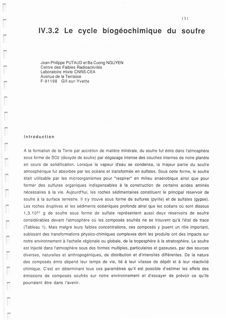
131
IV.3.2 Le cycle biogéochimique du soufre
Jean-Philippe PUTAUD et Ba Cuong NGUYEN Centre des Faibles Radioactivités Laboratoire mixte CNRS-CEA Avenue de la Terrasse F-91198 Gif-sur-Yvette
Introduction
A la formation de la Terre par accrétion de matière minérale, du soufre fut émis dans l'atmosphère
sous forme de S02 (dioxyde de soufre) par dégazage intense des couches internes de notre planète
en cours de solidification. Lorsque la vapeur d'eau se condensa, la majeur partie du soufre
atmosphérique fut absorbée par les océans et transformée en sulfates. Sous cette forme, le soufre
était utilisable par les microorganismes pour "respirer" en milieu anaérobique ainsi que pour
former des sulfures organiques indispensables à la construction de certains acides aminés
nécessaires à la vie. Aujourd'hui, les roches sédimentaires constituent le principal réservoir de
soufre à la surface terrestre. Il s·y trouve sous forme de sulfures {pyrite) et de sulfates (gypse).
Les roches éruptives et les sédiments océaniques profonds ainsi que les océans où sont dissous
1 ,3 .1 021 g de soufre sous forme de sulfate représentent aussi deux réservoirs de soufre
considérables devant l'atmosphère où les composés soufrés ne se trouvent qu'à l'état de trace
(Tableau 1 ). Mais malgré leurs faibles concentrations, ces composés y jouent un rôle important,
subissant des transformations physico-chimiques complexes dont les produits ont des impacts sur
notre environnement à l'echelle régionale ou globale, de la troposphère à la stratosphère. Le soufre
est injecté dans l'atmosphère sous des formes multiples, particulaires et gazeuses, par des sources
diverses, naturelles et anthropogéniques, de distribution et d'intensités différentes. De la nature
des composés émis dépend leur temps de vie, lié à leur vitesse de dépôt et à leur réactivité
chimique. C'est en déterminant tous ces paramètres qu'il est possible d'estimer les effets des
émissions de composés soufrés sur notre environnement et d'essayer de prévoir ce qu'ils
pourraient être dans l'avenir.
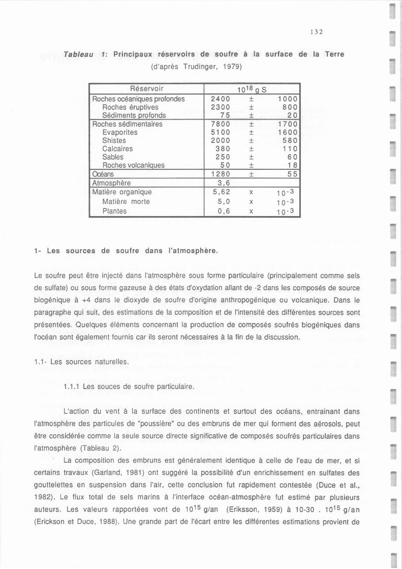
132
Tableau 1: Principaux réservoirs de soufre à la surface de la Terre
(d'après Trudinger, 1979)
Réservoir 1018 aS Roches océaniques profondes 2400 ± 1000
Roches éruptives 2300 ± 800 Sédiments profonds 75 ± 20
Roches sédimentaires 7800 ± 1700 Evaporites 5100 ± 1600 Shistes 2000 ± 580 Calcaires 380 ± 11 0 Sables 250 ± 60 Roches volcaniques 50 ± 1 8
Cœans 1280 ± 55 Atmosohère 3,6 Matière organique 5,62 X 1 o- 3
Matière morte 5,0 X 1 o- 3
Plantes 0,6 X 1 o- 3
1- Les sources de soufre dans l'atmosphère.
Le soufre peut être injecté dans l'atmosphère sous forme particulaire (principalement comme sels
de sulfate) ou sous forme gazeuse à des états d'oxydation allant de -2 dans les composés de source
biogénique à +4 dans le dioxyde de soufre d'origine anthropogénique ou volcanique. Dans le
paragraphe qui suit, des estimations de la composition et de l'intensité des différentes sources sont
présentées. Quelques éléments concernant la production de composés soufrés biogéniques dans
l'océan sont également fournis car ils seront nécessaires à la fin de la discussion.
1.1- Les sources naturelles.
1.1.1 Les souces de soufre particulaire.
L'action du vent à la surface des continents et surtout des océans, entrainant dans
l'atmosphère des particules de "poussière" ou des embruns de mer qui forment des aérosols, peut
être considérée comme la seule source directe significative de composés soufrés particulaires dans
l'atmosphère (Tableau 2).
La composition des embruns est généralement identique à celle de l'eau de mer, et si
certains travaux (Garland, 1981) ont suggéré la possibilité d'un enrichissement en sulfates des
gouttelettes en suspension dans l'air, cette conclusion fut rapidement contestée (Duce et al.,
1982). Le flux total de sels marins à l'interface océan-atmosphère fut estimé par plusieurs
auteurs. Les valeurs rapportées vont de 1015 g/an (Eriksson, 1959) à 10-30 . 1015 g/an
(Erickson et Duce, 1988). Une grande part de l'écart entre les différentes estimations provient de
,..
,...
133
la hauteur au-dessus de la mer à laquelle le flux a été calculé: entre 20 et 30 mètres, la
concentration en masse des sels marins décroit déja d'un facteur 2 (Blanchard et al., 1984) et au
niveau de la base des nuages, le nombre de particules de sels de mer est généralement inferieur à 1
cm-3 dans les zones océaniques (e.g. Andreae et al., 1986). En considérant que les sulfates
représentent 7,7% en masse des sels de mer, le flux de sulfates émis dans la couche 10-20
mètres au dessus de l'océan serait de 4, 1 à 8,6 Tmol/an (Varhelyi et Gravenhorst, 1983;
Blanchard, 1985). Cependant, le rayon moyen des particules d'aérosol de sels marins, en général
supérieur à 3 µm, leur confère une vitesse moyenne de dépot supérieur à 3 cm.s-1 (Erickson et
Duce, 1988) et donc un temps de vie atmosphérique relativement court qui leur interdit une
dissemination dans toute la couche limite marine. Ainsi, on estime génralement que la majorité des
particules de sels de mer se redépose rapidement à la surface des océans.
En ce qui concerne les aérosols terrigènes, la situation est assez comparable: les quantités
de matière transportées peuvent être considérables, et la formation par érosion éolienne
d'aérosols désertiques contenant du gypse (Ca S04 . 2 H20) est une source de sulfate importante
dans l'atmosphère. Mais le soufre d'origine crustal étant principalement contenu dans des
particules de rayon > 1 µm, ne peut, sauf événement exceptionnel, résider longtemps dans
l'atmosphère et atteindre l'altitude des nuages.
1 .1 .2- Les sources naturelles de composés soufrés gazeux.
1.1.2.1- Les sources "chaudes": volcans et feux de végétation.
Volcans et feux de végétation présentent deux caractéristiques communes: ce sont des
sources limitées dans le temps et l'espace qui émettent le soufre gazeux principalement sous
forme de S02 (tableau 2) . En revanche, si les sulfates ne constituent qu'une faible fraction du
soufre émis par les volcans, des mesures récentes effectuées dans des feux de végétation
pourraient suggérer que la moitié environ du S02 qu'ils émettent serait très rapidement convertie
en acide sulfurique (Nguyen et al., submitted). La spécificité majeure de la source volcanique
réside dans le fait que 7 % du soufre est émis lors d'éruptions explosives où le panache peut
atteindre la stratosphère (Stoiber et al., 1987), un monde physiquement et chimiquement très
différent de la troposphère où nous respirons.
1.1.2.2- Les sources biogéniques.
A l'exception de quelques sources ponctuelles mais très intenses (champs d'algues
côtiers, marais, etc ... ), les sources biogéniques telles que les océans, les sols et la végétation sont
diffuses mais étendues. La gamme de composés émis par ces sources comprend le sulfure
d'hydrogène (H2S), le sulfure de diméthyle (DMS), le disufure de carbone (CS2), l'oxysulfure de
carbone (COS), le disulfure de diméthyle (DMDS) et les mercaptans (R-SH). Certains des
134
processus conduisant à l'émission biogénique de ces composés sont encore mal connus. Cependant, 3
mécanismes ont été mis en évidence qui peuvent être effectifs dans différents milieux:
- décomposition des acides aminés dans les organismes vivants.
Dans le sol, les plantes et le plancton, ce mécanisme qui fait suite à l'assimilation des
sulfates afin de synthétiser les acides aminés soufrés, conduit à l'émission de OMS, CS2,
CH3SH et DMDS.
- réduction des sulfates par les bactéries
En milieu anaérobique (sols, eaux stagnantes ou profondes), les sulfates étant utilisés
comme oxydant de la matière organique sont réduits pour former très majoritairement
du H2S.
- dégradation photochimique des composés soufrés organiques.
Importante surtout à la surface des océans où l'oxydation des organe-soufrés dissous
constitue la principale source naturelle directe de COS dans l'atmosphère.
On conçoit aisément que les rendements de tous ces processus soit liés à certains
paramètres météorologiques tels que l'insolation ou la température. Et en effet, la production de
COS à la surface des océans présente un cycle journalier prononcé (amplitude d'un facteur 3 à 10)
avec un maximum autour de midi (Ferek and Andreae, 1984; Mihalopoulos et al., 1992). D'autre
part, les émissions de composés soufrés par les sols et les plantes croissent exponentiellement
avec la température (Goldan et al., 1987). Enfin, des variations saisonnières du flux de OMS à la
surface des océans, avec des maxima en été, ont été mises en évidence dans l'océan Pacifique, la
mer du Nord, et l'océan Indien (Bates et al., 1987a; Turner et al., 1988; Nguyen et al., 1990).
Mais il est hasardeux de déduire de ces observations l'existence d'éventuelles corrélations entre
production de OMS océanique et température ou insolation. Le relargage du OMS dans l'eau de mer
est en effet le fruit de processus biologiques complexes conduisant au clivage du dimethylsulfo-
propionate (DMSP: (CH3)2-S+-(CH2)2-COO·), synthétisé par les cellules phytoplanctoniques où
il aurait une fonction de régulation osmotique (Vairavamurthy et al., 1985). Et bien que le taux de
production de DMSP diffère suivant les espèces phytoplanctoniques (Keller et al., 1989), des
mesures effectuées dans divers régions océaniques ne montrent pas de corrélations claires entre
les concentrations de OMS dissous dans l'eau de mer et la distribution de ces espèces (Bates and
Cline, 1985; Bürgermeister et al., 1990; Leck et al., 1990). En fait, ce sont surtout l'état du
phytoplancton (sénéscence, broutage par le zooplancton; cf Dacey and Wakeham, 1986; Nguyen et
al., 1988; Belviso et al., 1991) et la dégradation du DMSP dissous dans l'eau de mer par des
bactéries (Kiene et Bates, 1990) qui semblent être les facteurs conduisant à la production de
OMS. L'inflence de paramètres physiques sur ces processus biologiques complexes n'étant pas
détrerminée, il est actuellement impossible de dire dans quel sens des variations de température
de l'eau de mer ou de l'insolation modifieraient la production de OMS dans les couches
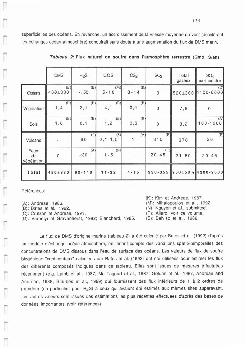
,...
135
superficielles des océans. En revanche, un accroissement de la vitesse moyenne du vent (accélérant
les échanges océan-atmosphère) conduirait sans doute à une augmentation du flux de OMS marin.
Tableau 2: Flux naturel de soufre dans l'atmosphère terrestre (Gmol Sian)
OMS
(B)
O::éans 480±330
(B)
Végétation 1 , 4
(B )
Sols 1 , 6
Volcans -
Feux œ 0
véaétation
Total 480±330
Références:
(A) : Andreae, 1986. (B): Bates et al., 1992.
H2S
(B
< 50
(B ,
2, 1
(B;
0, 1
(P;
60
(A;
<30
60-140
(C): Crutzen et Andreae, 1991.
cos c~
(M;
5 -1 0 3 -1 4
(B)
4, 1 0, 1
(B
1 , 2 0,3
(S
0,1-1,5 1
(N
1 - 5 -
11 - 2 2 4 -1 5
(0): Varhelyi et Gravenhorst, 1982; Blanchard, 1985.
(K:
(B;
(B;
(A)
S°'2 Total S04 gazeux particulaire
(D
0 520±360 14100-8600
0 7,8 0
(A'
0 3,2 100-1000
(P; (P,
310 370 20
(C; 2 0-45 21-80 2 0-4 5
330-355 950±50% 4200-9600
(K): Kim et Andreae, 1987. (M): Mihalopoulos et al., 1992. (N): Nguyen et al., submitted. (P): Allard, voir ce volume. (S): Belviso et al., 1986.
Le flux de OMS d'origine marine (tableau 2) a été calculé par Bates et al. (1992) d'après
un modèle d'échange océan-atmosphère, en tenant compte des variations spatio-temporelles des
concentrations de OMS dissous dans l'eau de surface des océans. Les valeurs de flux de soufre
biogénique "continentaux" calculées par Bates et al. (1992) ont été util isées pour estimer les flux
des différents composés indiqués dans ce tableau. Elles sont issues de mesures effectuées
récemment (e.g. Lamb et al., 1987; Mc Taggart et al., 1987; Goldan et al., 1987, Andreae and
Andreae, 1988, Staubes et al., 1989) qui fournissent des flux inférieurs de 1 à 2 ordres de
grandeur (en particulier pour H2S) à ceux qui avaient été estimés aux mêmes sites auparavant.
Les autres valeurs sont issues des estimations les plus récentes effectuées d'après des bases de
données importantes (voir références).
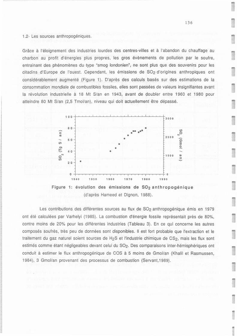
136
1.2- Les sources anthropogéniques.
Grâce à l'éloignement des industries lourdes des centres-villes et à l'abandon du chauffage au
charbon au profit d'énergies plus propres, les gros évènements de pollution par le soufre,
entrainant des phénomènes du type "smog londonien", ne sont plus que des souvenirs pour les
citadins d'Europe de l'ouest. Cependant, les émissions de SO2 d'origines anthropiques ont
considérablement augmenté (Figure 1 ). D'après des calculs basés sur des estimations de la
consommation mondiale de combustibles fossiles, elles sont passées de valeurs insignifiantes avant
la révolution industrielle à 18 Mt Sian en 1943, avant de doubler entre 1960 et 1980 pour
atteindre 80 Mt Sian (2,5 Tmollan), niveau qui doit actuellement être dépassé.
1 0 0 3000
80 • C ai
60
•• •• en • • ...o • • 2000 --" en • 3
C)
t:. 40 • 2.
• --N
0 en
20 • 1000 QI
:,
0 -+-r--r--r-ir-r-...,.......,-..-"T"""""T-,--....-,--r-....-,--r-.......-r-r--i--T-,-,-+- 0
1940 1950 1960 1970 1980 1990
Figure 1: évolution des émissions de S02 anthropogénique
(d'après Hameed et Oignon, 1988).
Les contributions des différentes sources au flux de SO2 anthropogénique émis en 1979
ont été calculées par Varhelyi (1985). La combustion d'énergie fossile représentait près de 80%,
contre moins de 20% pour les différentes industries (Tableau 3). En ce qui concerne les autres
composés soufrés, très peu de données sont disponibles. Il est fort probable que l'extraction et le
traitement du gaz naturel soient sources de H2S et l'industrie chimique de CS2, mais les flux sont
estimés comme étant négligeables devant celui du SO2. Des comparaisons inter-hémisphériques ont
conduit à estimer le flux anthropogénique de COS à 5 moins de Gmollan (Khalil et Rasmussen,
1984), 3 Gmollan provenant des processus de combustion (Servant, 1989).
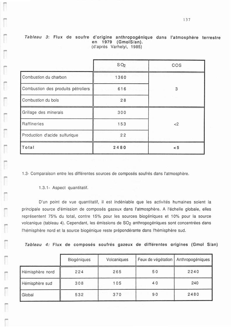
137
Tableau 3: Flux de soufre d'origine anthropogénique dans l'atmosphère terrestre en 1979 (GmolS/an). (d'après Varhelyi, 1985)
S°'2 cos
Combustion du charbon 1360
Combustion des produits pétroliers 616 3
Combustion du bois 28
Grillage des minerais 300
Raffineries 153 <2
Production d'acide sulfurique 22
Total 2480 <5
1.3- Comparaison entre les différentes sources de composés soufrés dans l'atmosphère.
1 .3 .1- Aspect quantitatif.
D'un point de vue quantitatif, il est indéniable que les activités humaines soient la
principale source d'émission de composés gazeux dans l'atmosphère. A l'échelle globale, elles
représentent 75% du total, contre 15% pour les sources biogéniques et 10% pour la source
volcanique (tableau 4). Cependant, les émissions de S02 anthropogéniques sont concentrées dans
l'hémisphère nord et la source biogénique reste prépondérante dans l'hémisphère sud.
Tableau 4: Flux de composés soufrés gazeux de différentes origines (Gmol Sian)
Biogéniques Volcaniques Feux de végétation Anthropogéniques
Hémisphère nord 224 265 50 2240
Hémisphère sud 308 105 40 240
Global 532 370 90 2480
138
Il faut également noter que dans d'immenses régions océaniques ou peu industrialisées,
ainsi que dans des zones côtières par exemple, l'atmosphère est alimentée par des sources
naturelles qui sont loin d'être négligeables devant les sources anthropiques. Pour y estimer
l'impact des émissions anthropogéniques sur le cycle naturel du soufre, il est important de
pouvoir déterminer l'origine des composés soufrés dans l'environnement. Or la plupart des
composés gazeux émis par les sources biogéniques est transformée en SO2 (cf paragraphe 2), qui
est aussi le principal gaz soufré d'origine volcanique et anthropogénique. Le SO2 est finalement
oxydé en acide sulfurique (H2SO4), dissocié et partiellement neutralisé pour donner des sulfates,
également contenus dans les aérosols d'origine crustale ou marine. L'analyse chimique ne permet
donc pas directement de déterminer l'origine des composés soufrés dans l'atmosphère ou les
précipitations.
1.3.2- Discrimination des différentes sources de soufre dans l'environnement.
Il est possible d'estimer la contribution des différentes sources des composés dans
l'environnement en mesurant dans les échantillons recueillis les concentrations d'autres espèces
caractéristiques de ces sources (des "traceurs") pour lesquelles on connait le rapport
SOx/traceur. Ainsi, la mesure de la concentration en Mg2+ dans un échantillon d'aérosol ou d'eau de
pluie permet, connaissant le rapport SO42-/Mg2+ dans l'eau de mer, de déterminer la contribution
des embruns marins à la teneur en sulfate observée dans cet échantillon. De même, on peut dans
certains cas utiliser le vanadium comme traceur des processus de combustion industrielle, le
potassium comme traceur des feux de végétation, etc ...
Une autre méthode de discrimination des sources de soufre dans l'environnement repose
sur la mesure du rapport isotopique du soufre dans les échantillons. Le soufre a en effet 4 isotopes
stables, dont le rapport entre les plus abondants est de l'ordre de 32 s134 s = 22,6. Le
fractionnement isotopique du soufre, produit principalement au cours d'équilibres ou de processus
biologiques d'oxyde-réduction des composés soufrés, conduit à enrichir ou appauvrir certains de
ses composés en l'isotope le plus lourd 34s. Ce fractionnement est défini par comparaison avec une
roche standard, la "Canyon Diablo Triolite" (CDT), dont la composition isotopique est proche de
celle des météorites. Généralement faible, le fractionnement est exprimé en "partie par milliers"
sous la forme suivante:
a34S (%0) =[(;:s1 :!S)échantillon - 1) X 1000 ( S/ S) référence
Les spectromètres de masse modernes permettent de comparer des échantillons contenant
environ 0,5 mg de soufre avec une précision de 0, 1o/oo (Thode, 1991 ).
On peut constater que le a34s est proche de o dans les composés qui n'ont pas participé à
des cycles biologiques telles que ceux contenus dans les silles basiques et ultrabasiques ou les
intrusions granitiques (figure 2). De même, les roches et gaz volcaniques ayant subi diverses
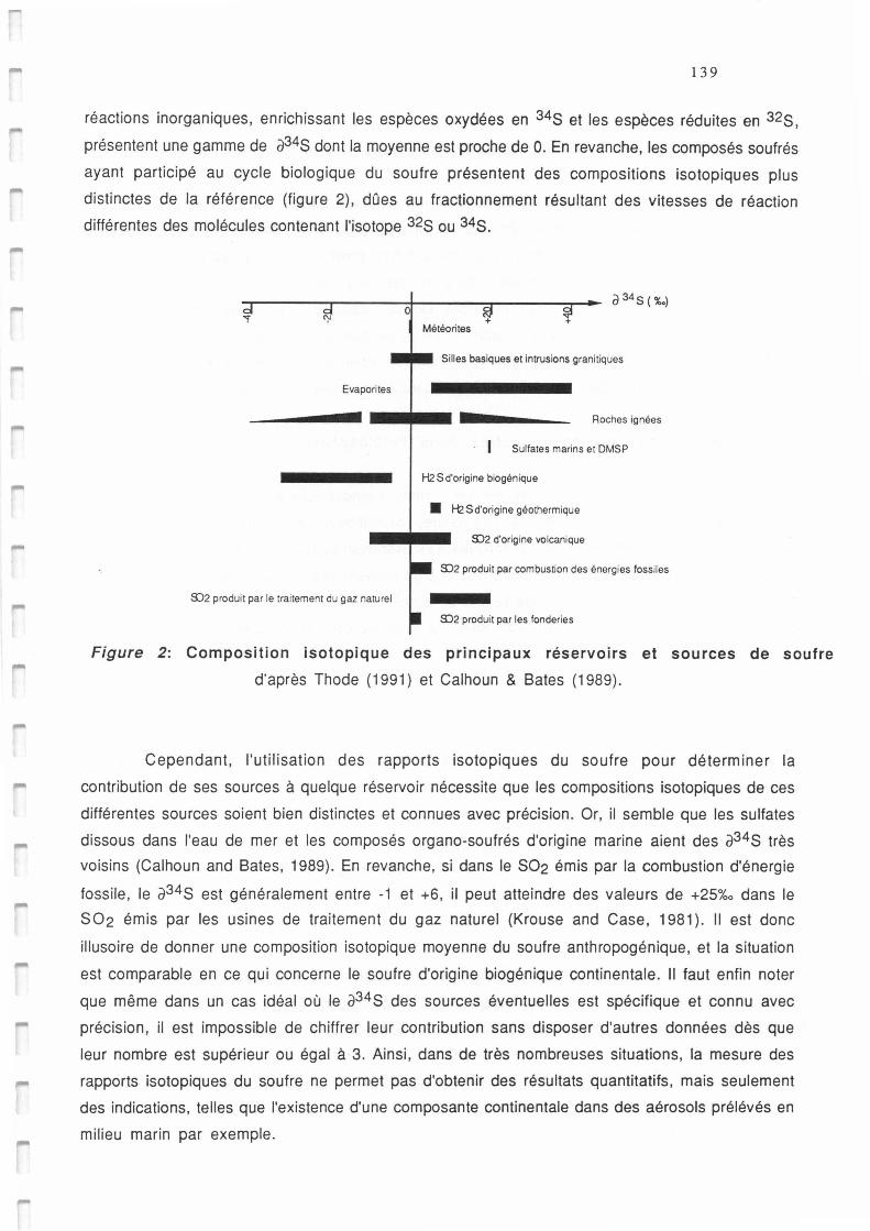
139
réactions inorganiques, enrichissant les espèces oxydées en 34s et les espèces réduites en 32s,
présentent une gamme de a34S dont la moyenne est proche de O. En revanche, les composés soufrés
ayant participé au cycle biologique du soufre présentent des compositions isotopiques plus
distinctes de la référence (figure 2), dûes au fractionnement résultant des vitesses de réaction
différentes des molécules contenant l'isotope 32s ou 34s.
0 +
Météorites
Silles basiques et intrusions granitiques
Evaporites
Roches ignées
Sulfates marins et DMSP
H2 S d'origine biogénique
• H2 $d'origine géothermique
5)2 d'origine volcanique
5)2 produit par combustion des énergies fossiles
S)2 produit par le traitement du gaz naturel
5)2 produit par les fonderies
Figure 2: Composition isotopique des principaux réservoirs et sources de soufre
d'après Thode (1991) et Calhoun & Bates (1989) .
Cependant, l'utilisation des rapports isotopiques du soufre pour déterminer la
contribution de ses sources à quelque réservoir nécessite que les compositions isotopiques de ces
différentes sources soient bien distinctes et connues avec précision. Or, il semble que les sulfates
dissous dans l'eau de mer et les composés organe-soufrés d'origine marine aient des a34s très
voisins (Calhoun and Bates, 1989). En revanche, si dans le S02 émis par la combustion d'énergie
fossile, le a34s est généralement entre -1 et +6, il peut atteindre des valeurs de +25%o dans le
S02 émis par les usines de traitement du gaz naturel (Krouse and Case, 1981). Il est donc
illusoire de donner une composition isotopique moyenne du soufre anthropogénique, et la situation
est comparable en ce qui concerne le soufre d'origine biogénique continentale. Il faut enfin noter
que même dans un cas idéal où le a34 s des sources éventuelles est spécifique et connu avec
précision, il est impossible de chiffrer leur contribution sans disposer d'autres données dès que
leur nombre est supérieur ou égal à 3. Ainsi, dans de très nombreuses situations, la mesure des
rapports isotopiques du soufre ne permet pas d'obtenir des résultats quantitatifs, mais seulement
des indications, telles que l'existence d'une composante continentale dans des aérosols prélévés en
milieu marin par exemple.
140
1 .3.3- Importance de la nature et du mode d'émission des composés soufrés.
Les diverses sources de soufre dans l'environnement diffèrent aussi d'un point de vue
qualitatif, par la nature des composés émis et l'altitude qu'ils peuvent atteindre. Il a été mentionné
plus haut que les sulfates émis directement sous forme particulaire dans les embruns ou les
aérosols crustaux ne pouvaient en général atteindre des altitudes très élévées à cause du rayon
moyen important de ces particules. En revanche, les composés émis lors d'éruptions volcaniques
explosives sont propulsés jusqu'à la stratosphère. En ce qui concerne les gaz émis au niveau du sol
par les sources naturelles et anthropogéniques, l'altitude atteinte et les effets sur l'environnement
dépendent étroitement de leur réactivité chimique dans l'atmosphère (cf paragraphes suivants).
2- Le devenir des composés soufrés dans l'atmosphère.
En général, tout composé soufré émis dans l'atmosphère est oxydé jusqu'au degré
maximum d'oxydation du soufre +6. Selon sa nature, l'oxydation se fera plus ou moins rapidement
et sous des conditions plus ou moins drastiques. Les mécanismes de réaction sont pour la plupart
encore mal connus mais l'étape d'initiation est le plus souvent une oxydation par le radical OH 0,
dont la concentration moyenne est de l'ordre de S. 105 molecule.cm-3 dans la troposphère. La
réaction conduisant de S02 (+4) aux composés où le soufre est à l'état d'oxydation +6 est traitée
dans le paragraphe 2.6.
2.1- Le sulfure d'hydrogène (H2S)
La principale réaction d'oxydation de H2S dans la troposphère résulte de l'arrachement
d'un atome d'hydrogène par le radical OH:
(2.1 .1)
02 + HS ---> OH + SO et/ou H02 + S
02 + S ---> 0 +SO
02 + SO ---> 0 + S02
La réaction (2.1.1) est l'étape limitante de la réaction. La constante cinétique de cette
réaction serait de 4,7. 10-12 cm3 .molecule-1 .s-1 (De More et al., 1985), conférant au sulfure
d'hydrogène un temps de vie légèrement inférieur à 5 jours dans la troposphère. Lors d'injection
de H2S dans la stratosphère au cours d'éruptions volcaniques, il est probable que la photo-
dissociation soit à l'origine de la réaction en chaîne d'oxydation de H2S schématisée ci-dessus.
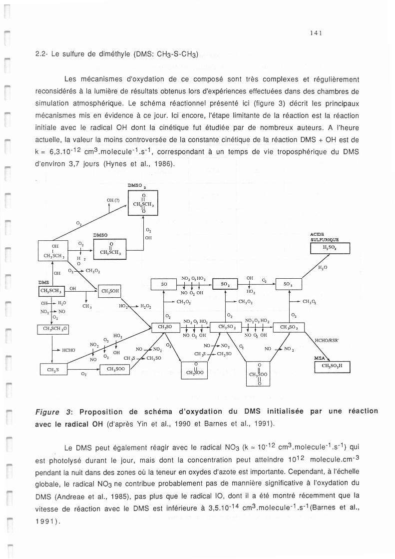
,..
14 1
2.2- Le sulfure de diméthyle (OMS: CH3-S-CH3)
Les mécanismes d'oxydation de ce composé sont très complexes et régulièrement
reconsidérés à la lumière de résultats obtenus lors d'expériences effectuées dans des chambres de
simulation atmosphérique. Le schéma réactionnel présenté ici (figure 3) décrit les principaux
mécanismes mis en évidence à ce jour. Ici encore, l'étape limitante de la réaction est la réaction
initiale avec le radical OH dont la cinétique fut étudiée par de nombreux auteurs. A l'heure
actuelle, la valeur la moins controversée de la constante cinétique de la réaction OMS + OH est de
k = 6 ,3.10- 12 cm3 .molecuie-1 .s-1, correspondant à un temps de vie troposphérique du OMS
d'environ 3 ,7 jours (Hynes et al., 1986).
OH(?)
OH
HCHO
CH3S
!DMSO 2
0 Il
CH3SCH 3 IJ
so
0
CH~OO
so,
Oz
OH 0,
HOz
CH 3 Oz
NOzO3 HOz
NO 0i OH
0
CH 3~00 Il 0
so,
Oz
CH-{,O 3
ACIDE
SUU'"'JJUQI.Œ
1-12s0,
CH 30z
CH3S03H
Figure 3: Proposition de schéma d'oxydation du DMS initialisée par une réaction
avec le radical OH (d'après Yin et al., 1990 et Barnes et al., 1991 ).
Le OMS peut également réagir avec le radical N03 (k"' 10-12 cm3.molecuie-1.s-1) qui
est photolysé durant le jour, mais dont la concentration peut atteindre 1012 molecule.cm- 3
pendant la nuit dans des zones où la teneur en oxydes d'azote est importante. Cependant, à l'échelle
globale, le radical N03 ne contribue probablement pas de mannière significative à l'oxydation du
OMS (Andreae et al., 1985), pas plus que le radical 10, dont il a été montré récemment que la
vitesse de réaction avec le OMS est inférieure à 3,s.10-14 cm3 .molecufe-1 .s- 1 (Barnes et al.,
1991).
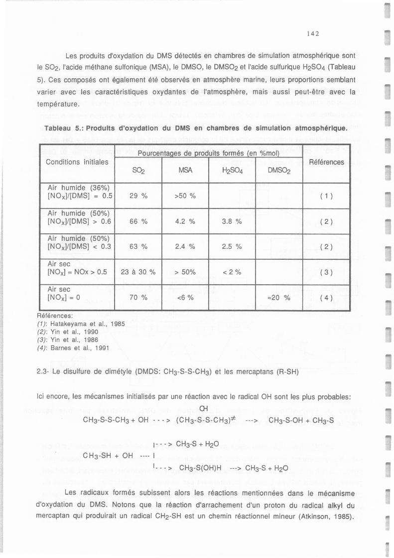
142
Les produits d'oxydation du OMS détectés en chambres de simulation atmosphérique sont
le SO2, l'acide méthane sulfonique (MSA), le OMSO, le OMSO2 et l'acide sulfurique H2SO4 (Tableau
5). Ces composés ont également été observés en atmosphère marine, leurs proportions semblant
varier avec les caractéristiques oxydantes de l'atmosphère, mais aussi peut-être avec la
température.
Tableau 5.: Produits d'oxydation du DMS en chambres de simulation atmosphérique.
Pourcentages de produits formés (en %mol) Conditions initiales
SÜ2
Air humide (36%) [NOx]/[OMS] = 0.5 29 %
Air humide (50%) [NOx]/[OMS] > 0.6 66 %
Air humide (50%) [NOx]/[OMS] < 0.3 63 %
Air sec [NOx] = NOx > 0.5 23 à 30 %
Air sec [NOx] = 0
Références : (1 ) : Hatakeyama et al., 1985 (2) : Yin et al., 1990 (3) : Yin et al. , 1986 (4): Barnes et al. , 1991
70 %
MSA H2SO4 OMSO2
>50 %
4.2 % 3.8 %
2.4 % 2.5 %
> 50% < 2%
<6 % :::::20 %
2.3- Le disulfure de dimétyle (DMOS: CH3-S-S-CH3) et les mercaptans (R-SH)
Références
( 1 )
( 2 )
( 2 )
( 3 )
( 4 )
Ici encore, les mécanismes initialisés par une réaction avec le radical OH sont les plus probables:
CH
CH3-S-S-CH3 + OH - - - > (CH3-S-S-CH3):;t ---> CH3-S-OH + CH3-S
1 - - - > CH3-S + H2O
C H3-SH + OH ---- 1
1- - - > CH3-S(OH)H ---> CH3-S + H2O
Les radicaux formés subissent alors les réactions mentionnées dans le mécanisme
d'oxydation du OMS. Notons que la réaction d'arrachement d'un proton du radical alkyl du
mercaptan qui produirait un radical CH2-SH est un chemin réactionnel mineur (Atkinson, 1985).
143
2.4- Le disulfure de carbone (CS2)
L'oxydation de CS2 par les radicaux OH ne peut se faire avec une vitesse significative
qu'en présence d'oxygène, selon 13 mécanismes possibles (Hynes et Wine, 1989), dont seule la
première étape semble établie, bien que la structure du complexe de transition formé soit encore
inconnue (M est un troisième corps inerte):
OH + CS2 + M <===> (CS2OH):t: + M
Quelques réactions envisageables pour les étapes suivantes sont décrites ici:
(CS2OH):t: + 02
et/ou
et/ou
- - - > SÜ2 + CO + SH
- - - > SO2 + COS + H
- - - > SH + COS + 02
Les radicaux SH formant finalement du SO2, les produits finaux de la réaction d'oxydation de CS2
seraient COS et SO2 (Barnes et al., 1983) en égales proportions, bien que la présence de CO dans
les produits de cette réaction ait été mise en évidence (Yang et al., 1987). L'oxydation de cs2
constitue donc une des sources de COS dans l'atmosphère. La constante cinétique de référence pour
la réaction CS2 + OH est de 1, 1. 10-12 cm3 .molecule-1 .s-1 (Hynes et Wine, 1989) correspondant
à un temps de vie moyen de CS2 de 21 jours dans la troposphère.
2.5- L'oxysulfure de carbone (COS)
Dans la troposphère, la seule réaction d'oxydation du COS décrite est:
COS+OH - - - > (COSOH):t: - - - > CO2 + SH , entre autres produits (2 .5.1)
Cette réaction est très lente puisqu'elle correspond à un temps de vie moyen du COS de 63
ans , très supérieur au temps de vie troposphérique du COS estimé d'après des mesures
atmosphériques à "' 2 ans . La stabilité de sa concentration dans la troposphére (autour de 500
pptv) montre que d'autres mécanismes conduisent à sa disparition , comme par exemple
l'absorption par la végétation (dépôt sec) ou les échanges avec la stratosphère, où les photons plus
énergétiques et les radicaux plus nombreux peuvent oxyder le COS selon les réactions suivantes
(Oppenheimer, 1987) :
COS+hv
COS+OH
COS+O
- - - > CO+ S
- - - > CO2 + SH + autres
- - - > CO+SO
(2 .5.2)
(2 .5.1)
(2.5 .3)
Aux latitudes moyennes , la réaction (2.5 .2) est le principal puits de COS: cette réaction
devient rapide au dessus de 25 km, où elle confère au COS un temps de vie inférieur à 1 jour
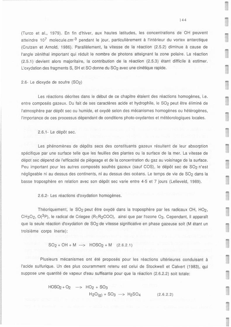
144
(Turco et al., 1979). En fin d'hiver, aux hautes latitudes, les concentrations de OH peuvent
atteindre 107 molecule.cm-3 pendant le jour, particulièrement à l'intérieur du vortex antarctique
(Crutzen et Arnold, 1986). Parallèlement, la vitesse de la réaction (2.5.2) diminue à cause de
l'angle zénithal important qui réduit le nombre de photons atteignant la zone polaire. La réaction
(2.5.1) devient alors majoritaire, la contribution de la réaction (2.5.3) étant difficile à estimer.
L'oxydation des fragments S, SH et SO donne du S02 avec une cinétique rapide.
2.6- Le dioxyde de soufre (S02)
Les réactions décrites dans le début de ce chapitre étaient des réactions homogènes, i.e.
entre composés gazeux. Du fait de ses caractères acide et hydrophile, le S02 peut être éliminé de
l'atmosphère par dépôt sec ou humide, et oxydé selon des mécanismes homogènes ou hétérogènes,
l'importance de ces processus dépendant de conditions photo-oxydantes et météorologiques locales.
2.6.1- Le dépôt sec.
Les phénomènes de dépôts secs des constituants gazeux résultent de leur absorption
spécifique par une surface telle que les feuilles des plantes ou la surface de la mer. La vitesse de
dépot sec dépend de l'efficacité de piégeage et de la concentration du gaz au voisinage de la surface.
Peu important pour les autres composés soufrés gazeux (sauf COS), le dépôt sec de S02 n'est
négligeable ni au dessus des continents, ni au dessus des océans. Le temps de vie de S02 dans la
basse troposphère en relation avec son dépôt sec varie entre 4-5 et 7 jours (Lelieveld, 1989).
2.6.2- Les réactions d'oxydation homogènes.
Théoriquement, le S02 peut être oxydé dans la troposphère par les radicaux OH, H02,
CH302, 0(3P), le radical de Criegee (R1 R2COO), ainsi que par l'ozone 03. Cependant, il apparaît
que la seule réaction d'oxydation de S02 de vitesse significative en phase gazeuse soit (M étant un
troisième corps inerte):
S02 + OH + M ---> HOS02 + M (2.6 .2.1)
Plusieurs mécanismes ont été proposés pour les réactions ultérieures conduisant à
l'acide sulfurique. Un des plus couramment retenu est celui de Stockwell et Calvert (1983), qui
suppose une quantité de vapeur d'eau suffisante pour que la réaction (2.6.2.2) soit totale:
H0SÜ2 + Û2 ---> H02 + S03
H20(g) + S03 ---> H2S04 (2 .6.2.2)
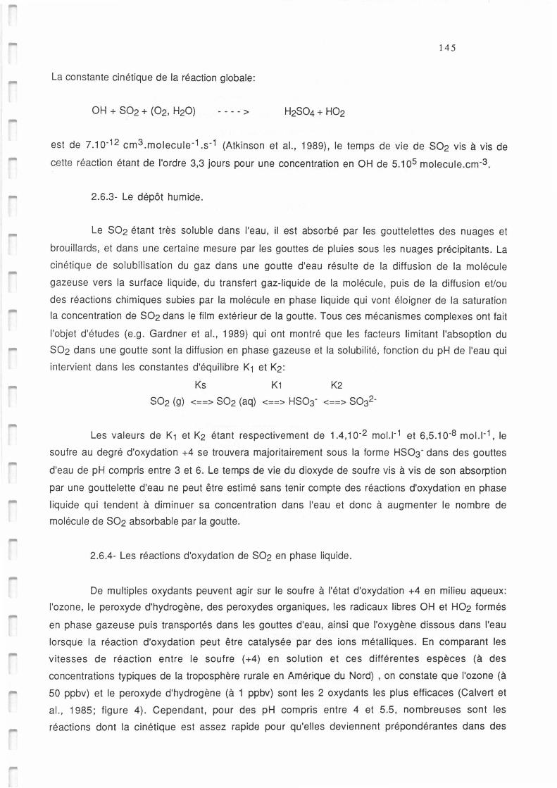
145
La constante cinétique de la réaction globale:
- - - - >
est de 7.10-12 cm 3.molecuie-1.s-1 (Atkinson et al., 1989), le temps de vie de SO2 vis à vis de
cette réaction étant de l'ordre 3,3 jours pour une concentration en OH de 5. 105 molecule.cm-3.
2.6.3- Le dépôt humide.
Le SO2 étant très soluble dans l'eau, il est absorbé par les gouttelettes des nuages et
brouillards, et dans une certaine mesure par les gouttes de pluies sous les nuages précipitants. La
cinétique de solubilisation du gaz dans une goutte d'eau résulte de la diffusion de la molécule
gazeuse vers la surface liquide, du transfert gaz-liquide de la molécule, puis de la diffusion eVou
des réactions chimiques subies par la molécule en phase liquide qui vont éloigner de la saturation
la concentration de SO2 dans le film extérieur de la goutte. Tous ces mécanismes complexes ont fait
l'objet d'études (e.g. Gardner et al., 1989) qui ont montré que les facteurs limitant l'absoption du
SO2 dans une goutte sont la diffusion en phase gazeuse et la solubilité, fonction du pH de l'eau qui
intervient dans les constantes d'équilibre K1 et K2:
Ks K1 K2
SO2 (g) <==> SO2 (aq) <==> HSO3- <==> SO32-
Les valeurs de K 1 et K2 étant respectivement de 1.4, 10-2 mo1.1- 1 et 6,5. 10-8 mo1.1- 1 , le
soufre au degré d'oxydation +4 se trouvera majoritairement sous la forme HSO3- dans des gouttes
d'eau de pH compris entre 3 et 6. Le temps de vie du dioxyde de soufre vis à vis de son absorption
par une gouttelette d'eau ne peut être estimé sans tenir compte des réactions d'oxydation en phase
liquide qui tendent à diminuer sa concentration dans l'eau et donc à augmenter le nombre de
molécule de SO2 absorbable par la goutte.
2.6.4- Les réactions d'oxydation de SO2 en phase liquide.
De multiples oxydants peuvent agir sur le soufre à l'état d'oxydation +4 en milieu aqueux:
l'ozone, le peroxyde d'hydrogène, des peroxydes organiques, les radicaux libres OH et HO2 formés
en phase gazeuse puis transportés dans les gouttes d'eau, ainsi que l'oxygène dissous dans l'eau
lorsqu'e la réaction d'oxydation peut être catalysée par des ions métalliques. En comparant les
vitesses de réaction entre le soufre (+4) en solution et ces différentes espèces (à des
concentrations typiques de la troposphère rurale en Amérique du Nord) , on constate que l'ozone (à
50 ppbv) et le peroxyde d'hydrogène (à 1 ppbv) sont les 2 oxydants les plus efficaces (Calvert et
al., 1985; figure 4). Cependant, pour des pH compris entre 4 et 5.5, nombreuses sont les
réactions dont la cinétique est assez rapide pour qu'elles deviennent prépondérantes dans des
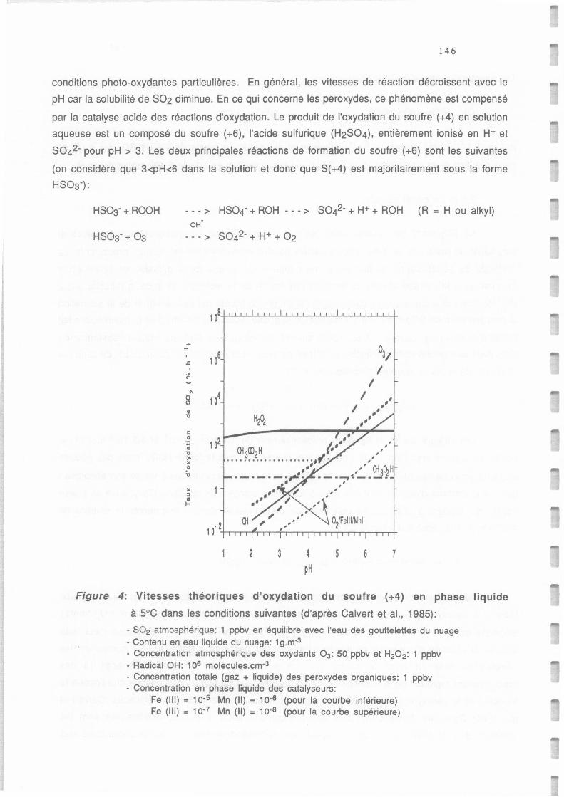
146
conditions photo-oxydantes particulières. En général, les vitesses de réaction décroissent avec le
pH car la solubilité de SO2 diminue. En ce qui concerne les peroxydes, ce phénomène est compensé
par la catalyse acide des réactions d'oxydation. Le produit de l'oxydation du soufre (+4) en solution
aqueuse est un composé du soufre (+6), l'acide sulfurique (H2SO4), entièrement ionisé en H+ et
SO42- pour pH > 3. Les deux principales réactions de formation du soufre (+6) sont les suivantes
(on considère que 3<pH<6 dans la solution et donc que S(+4) est majoritairement sous la forme
HSO3-):
HSD3-+ROOH - - - > HSO4- + ROH - - - > SO42- + H+ + ROH (R = H ou alkyl) OH
108
-03/
.. 106
.t:.
~ I .
I .. 10• I
~ u I "0
H2~ I C 0
1 o2 âi
, , , "0 , > , )C
, .o ,,,' Oi 3~H "0 -----,-----, , , )C , ::, . • >--
10·2 Oi
2 3 4 5 6 7 pH
Figure 4: Vitesses théoriques d'oxydation du soufre (+4) en phase liquide
à S°C dans les conditions suivantes (d'après Calvert et al., 1985):
- S02 atmosphérique: 1 ppbv en équilibre avec l'eau des gouttelettes du nuage - Contenu en eau liquide du nuage: 1g.m-3
- Concentration atmosphérique des oxydants 0 3 : 50 ppbv et H20 2 : 1 ppbv - Radical OH: 106 molecules.cm-3
- Concentration totale (gaz + liquide) des peroxydes organiques: 1 ppbv - Concentration en phase liquide des catalyseurs:
Fe (Ill) = 10-5 Mn (Il) = 10-6 (pour la courbe inférieure) Fe (Ill) = 10-7 Mn (Il) = 10-8 (pour la courbe supérieure)
147
2.6 .5- Les réactions d'oxydation de SO2 adsorbé sur des particules solides.
Les particules support d'oxydation peuvent être des particules de carbone (graphite ou
suie), de sels minéreaux d'origine marine ou crustale, des oxydes métalliques ou des aérosols
secondaires, issus de conversion gaz-particules de molécules organiques. La vitesse d'oxydation
dépend de la nature de la particule, de sa surface spécifique, et de l'humidité relative de l'air, ce
qui semble indiquer que la réaction a lieu dans le film liquide à la surface du solide. La fraction de
S O 2 oxydée selon ce processus est difficile à chiffrer. Elle pourrait être particulièrement
importante à proximité des sources d'émission de SO2 anthropogéniques où les concentrations de
particules sont élévées: dans une atmosphère où la densité des aérosols est de 100 µg.m-3, la
vitesse d'oxydation de SO2 sur les particules solides serait de 1 %.h- 1 (Baldwin, 1982). En
atmosphère marine chargée d'embruns, le taux de conversion de SO2 sur les aérosols pourrait
atteindre 5%.h- 1 (Sievering et al., 1991 ). Cependant, il est difficile dans de telles conditions de
distinguer les processus de "dépôt sec" (absoption par l'océan), de dépôt humide ou d'oxydation en
phase liquide, et d'oxydation sur les particules solides de sels marins, toujours très chargées
d'humidité.
2.7- Bilan de l'oxydation des composés soufrés.
En quelques étapes plus ou moins nombreuses, dans la troposphère ou la stratosphère, tout
composé soufré gazeux émis dans l'atmosphère est transformé en un produit dont la tension de
vapeur saturante est très faible et qui se trouve donc en grande partie dans la phase particulaire.
Outre le DMSO2, produit en très faible proportion par l'oxydation de sulfures organiques tels que
le OMS et le DMDS, les produits ultimes de ces transformations sont aussi des acides
(méthanesulfonique ou sulfurique) . Ces deux caractères (particulaires et acides) sont à l'origine
des effets des produits d'oxydation des composés soufrés sur notre environnement.
3- Interactions entre les composés soufrés et l'environnement terrestre.
3.1- Les composés soufrés dans la stratosphère.
Comme il l'a été indiqué dans les paragraphes précédents, les composés soufrés émis par
les volcans lors d'éruptions explosives peuvent fréquemment atteindre la stratosphère. En dehors
de ces injections massives, le COS émis depuis la surface de la Terre, dont le temps de vie
troposphérique est important (2 ans), est la principale source de soufre stratosphèrique
(Servant, 1986). Transformés en acide sulfurique, ces composés soufrés y affectent les réactions
chimiques et le bilan radiatif.
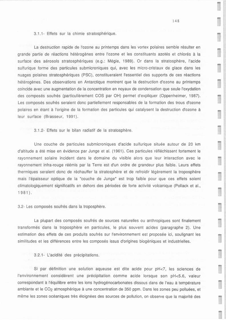
148
3.1.1- Effets sur la chimie stratosphérique.
La destruction rapide de l'ozone au printemps dans les vortex polaires semble résulter en
grande partie de réactions hétérogènes entre l'ozone et les constituants azotés et chlorés à la
surface des aérosols stratosphériques (e.g.: Mégie, 1989). Or dans la stratosphère, l'acide
sulfurique forme des particules submicroniques qui, avec les micro-cristaux de glace dans les
nuages polaires stratosphériques (PSC), constitueraient l'essentiel des supports de ces réactions
hétérogènes. Des observations en Antarctique montrent que la destruction d'ozone au printemps
coïncide avec une augmentation de la concentration en noyaux de condensation que seule l'oxydation
des composés soufrés (particulièrement COS par OH) permet d'expliquer (Oppenheimer, 1987).
Les composés soufrés seraient donc partiellement responsables de la formation des trous d'ozone
polaires en étant à l'origine de la formation des particules qui catalysent la destruction d'ozone à
leur surface (Brasseur, 1991 ).
3.1.2- Effets sur le bilan radiatif de la stratosphère.
Une couche de particules submicroniques d'acide sulfurique située autour de 20 km
d'altitude a été mise en évidence par Junge et al. (1961 ). Ces particules réfléchissent fortement le
rayonnement solaire incident dans le domaine du visible alors que leur interaction avec le
rayonnement infra-rouge réémis par la Terre est d'un ordre de grandeur plus faible. Leurs effets
thermiques seraient donc de réchauffer la stratosphère et de refroidir légèrement la troposphère
mais l'épaisseur optique de la "couche de Junge" est trop faible pour que ces effets soient
climatologiquement significatifs en dehors des périodes de forte activité volcanique (Pollack et al.,
1981).
3.2- Les composés soufrés dans la troposphère.
La plupart des composés soufrés de sources naturelles ou anthropiques sont finalement
transformés dans la troposphère en particules, le plus souvent acides (paragraphe 2). Une
estimation des effets de ces produits soufrés sur l'environnement est proposée ici, soulignant les
similitudes et les différences entre les composés issus d'origines biogéniques et industrielles.
3.2.1- L'acidité des précipitations.
Si par définition une solution aqueuse est dite acide pour pH<7, les sciences de
l'environnement considèrent une précipitation comme acide lorsque son pH<S.6, valeur
correspondant à l'équilibre entre les ions hydrogénocarbonates dissous dans de l'eau à température
ambiante et le C02 atmosphérique à une concentration de 350 ppm. Dans les zones peu polluées, et
même les zones océaniques très éloignées des sources de pollution, on observe que la majorité des
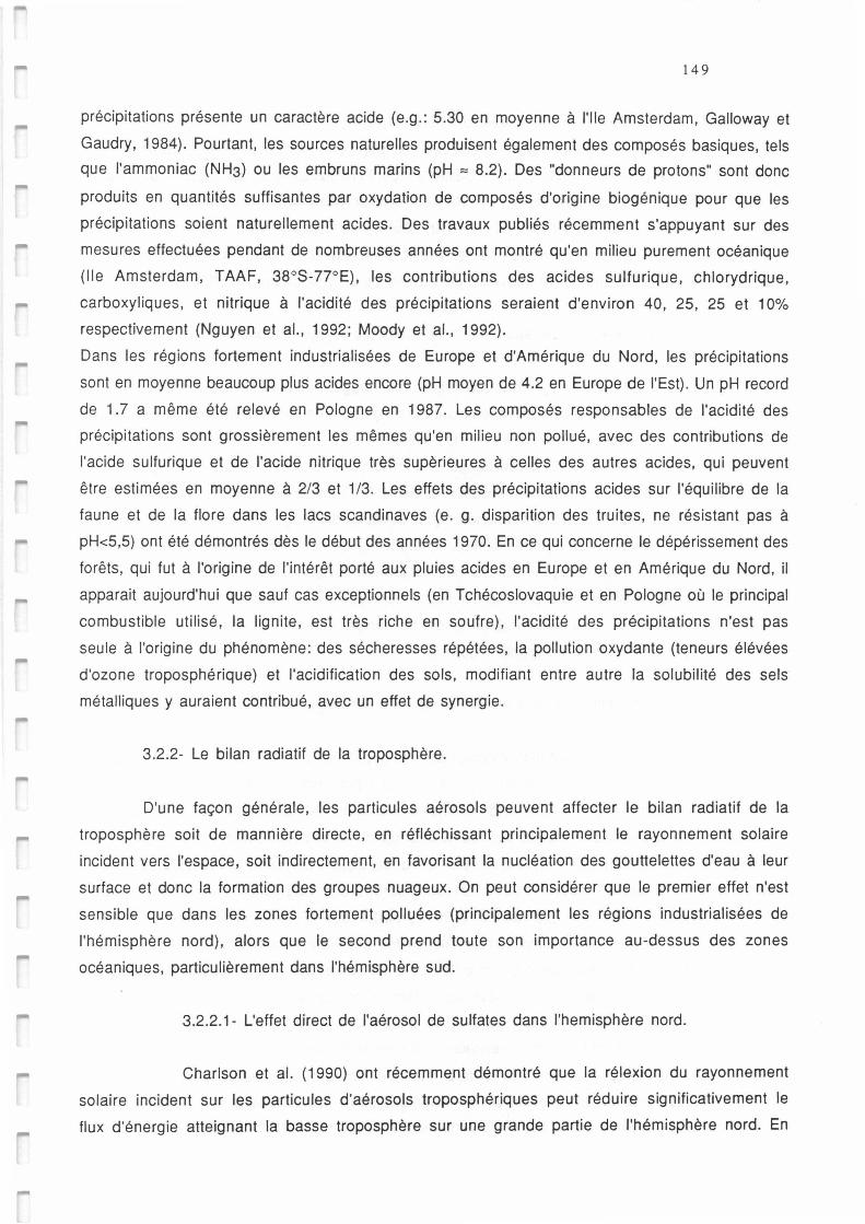
149
précipitations présente un caractère acide (e.g .: 5.30 en moyenne à l'lle Amsterdam, Galloway et
Gaudry, 1984). Pourtant, les sources naturelles produisent également des composés basiques, tels
que l'ammoniac (NH3) ou les embruns marins (pH == 8.2). Des "donneurs de protons" sont donc
produits en quantités suffisantes par oxydation de composés d'origine biogénique pour que les
précipitations soient naturellement acides. Des travaux publiés récemment s'appuyant sur des
mesures effectuées pendant de nombreuses années ont montré qu'en milieu purement océanique
(lie Amsterdam, TAAF, 38°S-77°E}, les contributions des acides sulfurique, chlorydrique,
carboxyliques, et nitrique à l'acidité des précipitations seraient d'environ 40, 25, 25 et 10%
respectivement (Nguyen et al., 1992; Moody et al., 1992).
Dans les régions fortement industrialisées de Europe et d'Amérique du Nord, les précipitations
sont en moyenne beaucoup plus acides encore (pH moyen de 4.2 en Europe de l'Est). Un pH record
de 1.7 a même été relevé en Pologne en 1987. Les composés responsables de l'acidité des
précipitations sont grossièrement les mêmes qu'en milieu non pollué, avec des contributions de
l'acide sulfurique et de l'acide nitrique très supèrieures à celles des autres acides, qui peuvent
être estimées en moyenne à 2/3 et 1/3. Les effets des précipitations acides sur l'équilibre de la
faune et de la flore dans les lacs scandinaves (e. g. disparition des truites, ne résistant pas à
pH<5,5) ont été démontrés dès le début des années 1970. En ce qui concerne le dépérissement des
forêts , qui fut à l'origine de l'intérêt porté aux pluies acides en Europe et en Amérique du Nord, il
apparait aujourd'hui que sauf cas exceptionnels (en Tchécoslovaquie et en Pologne où le principal
combustible utilisé, la lignite, est très riche en soufre), l'acidité des précipitations n'est pas
seule à l'origine du phénomène: des sécheresses répétées, la pollution oxydante (teneurs élévées
d'ozone troposphérique) et l'acidification des sols, modifiant entre autre la solubilité des sels
métalliques y auraient contribué, avec un effet de synergie .
3.2.2- Le bilan radiatif de la troposphère.
D'une façon générale, les particules aérosols peuvent affecter le bilan radiatif de la
troposphère soit de mannière directe, en réfléchissant principalement le rayonnement solaire
incident vers l'espace, soit indirectement, en favorisant la nucléation des gouttelettes d'eau à leur
surface et donc la formation des groupes nuageux. On peut considérer que le premier effet n'est
sensible que dans les zones fortement polluées (principalement les régions industrialisées de
l'hémisphère nord) , alors que le second prend toute son importance au-dessus des zones
océaniques, particulièrement dans l'hémisphère sud.
3.2.2.1- L'effet direct de l'aérosol de sulfates dans l'hemisphère nord.
Charlson et al. (1990) ont récemment démontré que la rélexion du rayonnement
solaire incident sur les particules d'aérosols troposphériques peut réduire significativement le
flux d'énergie atteignant la basse troposphère sur une grande partie de l'hémisphère nord. En
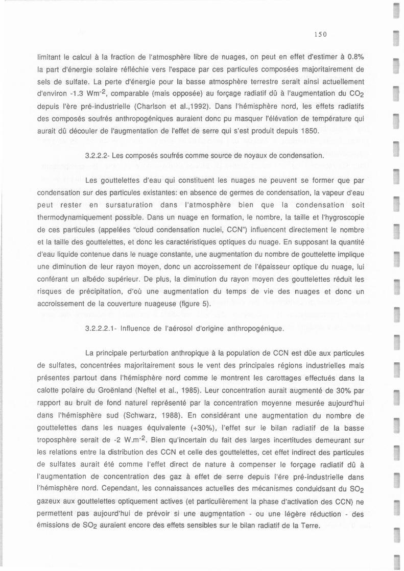
150
limitant le calcul à la fraction de l'atmosphère libre de nuages, on peut en effet d'estimer à 0.8%
la part d'énergie solaire réfléchie vers l'espace par ces particules composées majoritairement de
sels de sulfate. La perte d'énergie pour la basse atmosphère terrestre serait ainsi actuellement
d'environ -1.3 wm-2, comparable (mais opposée) au forçage radiatif dû à l'augmentation du C02
depuis l'ère pré-industrielle (Charlson et al., 1992). Dans l'hémisphère nord, les effets radiatifs
des composés soufrés anthropogéniques auraient donc pu masquer l'élévation de température qui
aurait dû découler de l'augmentation de l'effet de serre qui s'est produit depuis 1850.
3.2.2.2- Les composés soufrés comme source de noyaux de condensation.
Les gouttelettes d'eau qui constituent les nuages ne peuvent se former que par
condensation sur des particules existantes: en absence de germes de condensation, la vapeur d'eau
peut rester en sursaturation dans l'atmosphère bien que la condensation soit
thermodynamiquement possible. Dans un nuage en formation, le nombre, la taille et l'hygroscopie
de ces particules (appelées "cloud condensation nuclei, CCN") influencent directement le nombre
et la taille des gouttelettes, et donc les caractéristiques optiques du nuage. En supposant la quantité
d'eau liquide contenue dans le nuage constante, une augmentation du nombre de gouttelette implique
une diminution de leur rayon moyen, donc un accroissement de l'épaisseur optique du nuage, lui
conférant un albédo supérieur. De plus, la diminution du rayon moyen des gouttelettes réduit les
risques de précipitation, d'où une augmentation du temps de vie des nuages et donc un
accroissement de la couverture nuageuse (figure 5).
3.2.2.2.1- Influence de l'aérosol d'origine anthropogénique.
La principale perturbation anthropique à la population de CCN est dûe aux particules
de sulfates, concentrées majoritairement sous le vent des principales régions industrielles mais
présentes partout dans l'hémisphère nord comme le montrent les carottages effectués dans la
calotte polaire du Groënland (Neftel et al., 1985). Leur concentration aurait augmenté de 30% par
rapport au bruit de fond naturel représenté par la concentration moyenne mesurée aujourd'hui
dans l'hémisphère sud (Schwarz, 1988). En considérant une augmentation du nombre de
gouttelettes dans les nuages équivalente (+30%), l'effet sur le bilan radiatif de la basse
troposphère serait de -2 W.m-2. Bien qu'incertain du fait des larges incertitudes demeurant sur
les relations entre la distribution des CCN et celle des gouttelettes, cet effet indirect des particules
de sulfates aurait été comme l'effet direct de nature à compenser le forçage radiatif dû à
l'augmentation de concentration des gaz à effet de serre depuis l'ére pré-industrielle dans
l'hémisphère nord. Cependant, les connaissances actuelles des mécanismes conduidsant du S02
gazeux aux gouttelettes optiquement actives (et particulièrement la phase d'activation des CCN) ne
permettent pas aujourd'hui de prévoir si une augm~ntation - ou une légère réduction - des
émissions de S02 auraient encore des effets sensibles sur le bilan radiatif de la Terre.
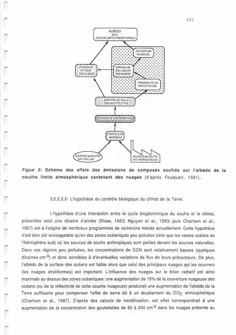
ALBEDO DELA
COUCHE LIMITE ATMOSPHERIQUE
15 1
Figue 5: Schéma des effets des émissions de composés soufrés sur l'albédo de la
couche limite atmosphérique contenant des nuages (d'après Fouquart, 1991 ).
3 .2.2.2.2- L'hypothèse du contrôle biologique du climat de la Terre.
L'hypothèse d'une interaction entre le cycle biogéchimique du soufre et le climat,
présentée voici une dizaine d'année (Shaw, 1983; Nguyen et al., 1983; puis Charlson et al. ,
1987) est à l'origine de nombreux programmes de recherche menés actuellement. Cette hypothèse
n'est bien sûr envisageable qu'en des zones océaniques peu polluées (telle que les vastes océans de
l'hémisphère sud) où les sources de soufre anthropiques sont petites devant les sources naturelles.
Dans ces régions peu polluées, les concentrations de CCN sont relativement basses (quelques
dizaines.cm-3) et donc sensibles à d'éventuelles variations de flux de leurs précurseurs. De plus,
l'albédo de la surface des océans est faible alors que celui des principaux nuages qui les couvrent
(les nuages stratiformes) est important. L'influence des nuages sur le bilan radiatif est ainsi
maximale au dessus des zones océaniques: une augmentation de 15% de la couverture nuageuse des
océans (ou de la réflectivité de cette couche nuageuse) produirait une augmentation de l'albédo de la
Terre suffisante pour compenser l'effet de serre dû à un doublement du C02 atmosphérique
(Charlson et al., 1987). D'après des calculs de modélisation, cet effet correspondrait à une
augmentation de la concentration des gouttelettes de 50 à 200 cm-3 dans les nuages présents au
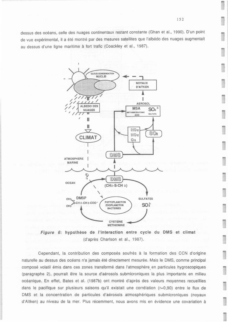
15 2
dessus des océans, celle des nuages continentaux restant constante (Ghan et al., 1990). D'un point
de vue expérimental, il a été montré par des mesures satellites que l'albédo des nuages augmentait
au dessus d'une ligne maritime à fort trafic (Coackley et al., 1987).
/ Il Il
è ATMOSPHERE
MARINE
1
CH,+ DMSP ,.S-CH 2 -CH 2-COO • PHYTOPLANCTON
NOYAUX D'AITKEN
AEROSOL
MSA METHANE.SlLFONtC
AOD
50i2-SULFATE
IXl@ii: 1--..,. ------....
OO@ii:
@3
SULFATES
CH3 t \ ZOOPLANCTON
'-- OAC,effl,S / )
CYSTEINE ..../· METHIONINE
Figure 6: hypothèse de l'interaction entre cycle du DMS et climat
(d'après Charlson et al., 1987).
Cependant, la contribution des composés soufrés à la formation des CCN d'origine
naturelle au dessus des océans n'a jamais été directement mesurée. Mais le OMS, comme principal
composé volatil émis dans ces zones transformé dans l'atmosphère_ en particules hygroscopiques
(paragraphe 2), pourrait être la source d'aérosols submicroniques la plus importante en milieu
océanique. En effet, Bates et al. (1987b) ont montré d'après des valeurs moyennes recueillies
dans le pacifique sur plusieurs saisons qu'il existait une corrélation (r=0,90) entre le flux de
OMS et la concentration de particules d'aérosols atmosphériques submicroniques (noyaux
d'Aïtken) au niveau de la mer. Plus récemment, nous avons mis en évidence une covariation à
153
court terme (24 h) entre la concentation de OMS atmosphérique et celle des noyaux d'Aïtken,
précurseurs directs des CCN (Nguyen et al., 1991 ). Ainsi, bien que les relations liant flux de
OMS, population de CCN, distribution des gouttelettes dans les nuages et bilan radiatif de
l'atmosphère ne soient pas toutes clairement établies , il serait donc possible que le flux des
composés soufrés d'origine naturelle influençât le climat de la Terre (Figure 6).
Le fait que la production des composés soufrés dans les océans soit peut-être dépendante de
paramètres climatiques (température, insolation) accroit encore l'intérêt présenté par la source
planctonique de soufre: en supposant qu'un réchauffement des eaux océaniques superficielles,
résultant de l'augmentation de l'effet de serre, entraine un accroissement du flux de OMS à la
surface des océans et donc de la réflectivité de la couche nuageuse océanique, l'effet radiatif
engendré s'opposerait à l'effet de serre croissant. Les relatives baisses d' insolation et de
température qui s'ensuivraient ralentiraient à leur tour la production de OMS. On serait donc en
présence d'un systême OMS-climat autorégulé , hypothèse chère à James Lovelock, auteur du
concept "Gaïa" (1979, 1986). Cependant , les mesures de S04 2- et de MSA effectuées dans les
carottes de glace prélevées en Antarctique montrent une augmentation de concentration de ces
composés pendant les périodes glacières (Legrand et al. , 1991 ). Bien qu'il soit hasardeux
d'interpoler ces données pour prévoir l'effet d'un réchauffement sur l'évolution de la production
de soufre biogén ique, ces résultats tendraient à montrer que les conséquences de l'effet de serre
pourraient être encore amplifiées par une diminution du flux de OMS naturel , qui, si l'on en croit
l'hypothèse de Charlson, entrainerait une réduction de l'albédo de la couche nuageuse océanique.
Comme on peut le voir, il reste beaucoup de chemin à parcourir pour comprendre les interactions
entre cycle du soufre et climat de mannière à pouvoir prédire leurs évolutions à venir.
Conclusion
Une chose est certaine: les rejets de dioxyde de soufre (S02) anthropogéniques représentent une
formidable perturbation du cycle biogéochimique du soufre à l'échelle globale. Cependant, dans
d 'immenses régions telles que les océans de l'hémisphère sud, les sources naturelles et
principalement la production de sulfure de diméthyl (OMS) par le plancton demeurent
prépondérantes. Et puis les chiffres ne disent pas tout: les effets des composés soufrés sur
l'environnement planétaire dépendent surtout de leur réactivité chimique et de la nature de leurs
sources. Ainsi, la stabilité de l'oxysulfure de carbone (COS), dont le flux principalement d'origine
naturelle est relativement faible, lui permet d 'atteindre la stratosphère où des photons plus
énergétiques le photolysent, initialisant sa transfomation en acide sulfurique. Les sources
naturelles, comprenant les émissions de composés soufrés (S02 et H2S) lors d'éruptions
volcaniques explosives, constituent ainsi le principal apport de soufre à la couche de
microcristaux d 'acide sulfurique stratosphériques qui présentent des interactions potentielles
avec le bilan radiatif de la Terre et la chimie de l'ozone. Cependant, il est vrai que la plupart des
154
composés soufrés, qu'ils soient d'origine naturelles ou anthropogéniques, sont oxydés dans la
troposphère pour y former majoritairement des aérosols d'acide sulfuriques. Ces aérosols servent
de noyaux de condensation lors de la formation des nuages et sont donc lessivés par les
précipitations. On connait les effets d'importants rejets de SO2 sur l'acidification des pluies dont
l'impact sur les écosystèmes peut être dramatique. Dans ce domaine, le rôle des émissions
naturelles est modeste bien que réel. De même, l'effet radiatif de rétrodiffusion du rayonnement
solaire incident par les particules de sulfates anthropogéniques a pu être estimé comme étant
suffisant pour avoir compensé l'augmentation de l'effet de serre dans l'hémisphère nord, alors
qu'il semble aujourd'hui insignifiant dans l'hémisphère sud. En ce qui concerne l'influence des
émissions des composés soufrés sur les caractéristiques optiques des nuages, de vastes incertitudes
demeurent. La formule reliant la taille des gouttelettes d'un nuage et son albédo est bien connue,
mais les relations entre la concentration des germes potentiels et le spectre de taille des
gouttelettes d'un nuage demeurent mal comprises. Il semble cependant qu'une augmentation du flux
de OMS à la surface des océans, entrainant un accroissement sensible de la concentration des
noyaux de condensation, conduirait à une augmentation de l'albédo de la couverture nuageuse au
dessus des zones océaniques non polluées. Toutes les mesures s'accordant pour montrer que la
production biogénique de OMS est maximale en été (maximum de température et d'insolation), on
peut voir dans ces deux phénomènes des indices de l'existence d'un processus d'auto-régulation
biologique du climat de la Terre. Cependant, les archives glaciologiques tendent à montrer que la
production de soufre biogénique fut maximale dans les périodes glacières ... Mais quoiqu'elles
furent dans le passé, les relations entre le cycle naturel des composés soufrés et le climat de notre
planète seraient aujourd'hui profondément perturbées par les émissions de SO2
anthropogéniques, tout au moins dans l'hémisphère nord où vivent la plupart des hommes.
Bibliographie:
Andreae, M.O. (1986). The ocean as a source of atmospheric sulfur compounds, in The Role of Air-Sea Exchange in Geochemical Cycling, edited by P. Buat-Ménard, O.Reidel, Hingham, Mass., 331-362.
Andreae, M.O. (1991 ). Biomass burning: its history, use, and distribution and its impact on environmental quality and global climate, in Global Biomass Burning, edited by J.S Levine, The MIT press, 1-21.
Andreae, M.O., Ferek, R.J., Bermond, F., Byrd, K.P., Engstrom, R.T., Hardin, S., Houmere, P.O., LeMarrec, F., Raemdonck, H. and Chatfield, R.B. (1985). Oimethylsulfide in the marine atmosphere, J. Geophys. Res. 90, 12891-12900.
Andreae M.O. and Andreae T.W. (1988). The cycle of biogenic sulfur compounds over the Amazon bassin in the dry season.J. Geophys. Res. 93, 1487-1497.
Andreae M.O., Charlson, R.J., Bruyseels, F., Storms, H., Van Grieken, R., Maenhaut, W. (1986). Salts, silicates and sulfates: internai mixture in marine aerosols. Science, 232, 7 44-7 4 7.
Atkinson R. (1985). Kinetics and mechanisms of the gas phase reaction of the OH radical with organic compounds under atmospheric conditions, Chem. Rev., 85, 69-79.
155
Atkinson, R., Baulch, D.L., Cox, R.A., Hampson, R.F. Jr, Kerr, J.A., Troe, J. (1989). Evaluated kinetic and photochemical data for atmospheric chemistry: supplement Ill, J. Phys. Chem. Data, 18, 881-1097.
Baldwin, A.C. (1982). Heterogeneous reactions of sulfur dioxide with carbonaceousparticles. /nt. J. Chem. Kin., 14, 269-274.
Barnes, 1., Becker, K.H ., Fink, E.H., Reimer, A. , Zabel, F., Niki, H. (1983). Rate constant and products of the reaction CS2+ OH in the presence of 02, /nt. J. Chem. Kin. 15, 631-639.
Barnes, 1., Bastian, V., Becker, K.H. (1988). Kinetics and mechanisms of the reaction of OH radicals with dimethyl sulfide, /nt. J. Chem. Kin. 20, 415-431.
Barnes, 1., Bonsang, B., Brauers, T., Carlier, P., Cox, R.A., Dorn, H.P., Jenkin, M.E., Le Bras, G., Platt, U. (1991 ). Laboratory and field syudies of oxidation processes occuring in the atmospheric marine boundary layer, Air Pollution Research Report 35 of the Environmental Reasearch Programme of the Commission of the European Communities, edited by Le Bras G.
Bates, T.M. and Cline, J.O. (1985). The role of the ocean in a regional sulfur cycle. J. Geophys. Res. 93, 9168-9172 .
Bates, T.M., Cline, J.O., Gammon R.H . and Kelly-Hansen , S.R. (1987a) . Regional and seasonal variation of the flux of oceanic dimethylsulfide to the atmosphere, J. Geophys. Res. 92, 2930-2938.
Bates, T.M., Charlson, R.J . and Gammon R.H. (1987b). Evidence for the climatic role of marine biogenic sulphur, Nature 329, 319-321.
Bates, T.S., Lamb, B.K. , Guenther, A.B. , Oignon, J., Stoiber, E.S. (1992). Sulfur emissions to the atmosphere from natural sources, J. Atmos. Chem. , in press.
Belviso, S., Nguyen , B.C., Allard, P. (1986). Estimate of carbonyl sulfide (OCS) volcanic source strength deduced from OCS/CO2 ratios in volcanic gases. Geophys. Res. Letts., 13, 133-136.
Belviso , S., Kim, S.K., Rassoulzadegan, F., Krajka, B., Nguyen, B.C., Mihalopoulos, N. , and Buat-Menard, P. (1991 ). Production of dimethylsulfonium propionate (DMSP) and dimethylsulfide (OMS) by the microbial food web, Limnol. Oceanogr., 35, 1810-1821.
Blanchard, D.C. , Woodcock, A.H ., Cipriano, R.J. (1984). The vertical distribution of the concentration of sea sait in marine atmosphere near Hawaii. Tel/us, 368, 118-125.
Blanchard, D. C. (1985). The oceanic production of atmospheric sea sait , J. Geophys. Res., 92, 961 -963 .
Brasseur, G.P. (1991 ). A deepening, broadening trend. Nature, 352, 668-669. Bürgermeister, S., Zimmerman, R.L., Georgii , H.W., Bingemer, H.G., Kirst, G.O., Jansen, M.,
Ernst, W. (1990). On the biogenic origin of dimethylsulfide: relation between chlorophyll, ATP, organismic DMSP, phytoplancton species, and OMS distribution in Atlantic surface seawater and atmosphere.J. Geophys. Res. 92, 2930-2938.
Calhoun, J.A. and Bates, T.S. (1989). Sulfur isotope ratios, in Biogenic Su/fur in the Environment, edited by Saltzman E.S. and Cooper W.J., American Chemical Society Symposium Series N° 393, Washigton DC, 367-378.
Crutzen, P. and Andreae , M.O, (1990) Biomass burning in tropics: impact on Atmospheric chemistry and biogeochemical cycles, Science, 250, 1669-1678. Calvert, J.G. , Larzus, A., Kok, L.G. , Heikes, B.G., Walega , J.G., Lind, J. , Cantrell, C.A. (1985) .
Chemical mechanisms of acid generation in the troposphere. Nature, 317, 27-35. Calvert, J.G. and W.R. Stockwell (1983). Acid generation in the troposphere by gas-phase
chemistry. Envir. Sei. Tech no/. 17, 428A-433A. Charlson R.J., Lovelock J.E., Andreae M.O., Warren S.G. (1987). Oceanic phytoplankton ,
atmospheric sulphur, cloud albedo and climate, Nature 326, 655-661 . Charlson R.J ., Langner, J., Rhode, H. (1990). Sulfate aerosol and climate, Nature, 348, 22. Charlson R.J ., Schwartz, S.E., Hales, J.M., Cess, R.D., Coackley, J.A.Jr, Hansen, J.E., Hoffman, D.J.
(1992). Climate forcing by anthropogenic aerosols. Science, 255, 423-430. Coackley, J.A.Jr, Bernstein, R.L., Durkee, P.A. (1987) . Effect of ship track effluents on cloud
reflectivity. Science 23 7, 1 020-1 022. Crutzen, P.J. and Arnold, F. (1986). Nitric acid cloud formation in the cold Antarctic stratosphere:
a major cause of the "ozone hole", Nature, 324, 651-655. Dacey, J.W.H. and Wakeham, S.G. (1986). Oceanic dimethylsulfide: production during zooplankton
grazing on phytoplankton, Science, 233 , 1314-1316. Duce, R.A., Mc lntyre, F. and Bonsang, B. (1982) . Enrichement of sulfate in maritime aerosols.
(Discussion) Atmos. Environ., 16, 2025-2034 .
156
Erickson, D.J., and Duce R.A. (1988). On the global flux of atmospheric sea sait, J.Geophys. Res. 93, 140 7 9-140 8 8.
Eriksson, E. (1959). The yearly circulation of chloride and sulfur in nature: meteorological, geochemical, and pedological implications. Part 1. Tel/us, 11, 375-403.
De More, W.B., Margitan, J.J., Molina, M.J., Watson, R.T., Golden, D.M., Hampson, R.F., Kurylo, M.J., Howard, C.J., Ravishankara, A.R. (1985). Chemical kinetics and photochemical data for use in stratospheric modelling, Evaluation N°7, NASNJPL publication85-37.
Ferek, R.J. and Andreae, M.O. (1984). Photochemical production of carbonyl sulfide in marine surface waters. Nature, 307, 148-150.
Fouquart, Y. (1991 ). Marine aerosol particules, CCNs, clouds and climate, Report to WCRP/JSC, Bremen, march 18-23, 1991.
Galloway, J.N. and Gaudry, A. (1984). The composition of precipitation on Amsterdam Island, lndian Ocean, Atmosph. Environ., 18, 2649-2656.
Gardner, J.A., Watson, L.R., Adewuyi, Y.J., Van Doren, J.M., Davidovits, P., Worsnop, D.R., Zahniser, M.S., Kolb, C.E. (1989). The uptake of Gases by liquid droplets, in Biogenic Su/fur in the Environment, edited by Saltzman E.S. and Cooper W.J., American Chemical Society Symposium Series N° 393, Washigton DC, 504-517.
Garland, J.A. (1981). Enrichement of sulfate in maritime aerosols. Atmos. Environ., 15, 787-791.
Ghan, S.J., Taylor, K.E., Penner, D.J., Erickson, D.J. (1990). Madel test of CCN-cloud albedo climate forcing. Geophys. Res. Lett., 17, 607-617.
Goldan, P.D., Kuster, W.C., Albritton, D.L., Fehsenfeld, F.C. (1987). The measurement of natural sulfur emissions from soils and vegetation: three sites in the eastern United States revisited. J. Atmos. Chem., 5, 439-467.
Hameed, S. and Oignon, J. (1988). Changes in the geographical distributions of global emissions of NOx and SOx from fossil fuel combustion between 1966 and 1980. Atmos. Environ.,22, 441-449.
Hynes, A.J., Wine, P .H., Semmes D.H. (1986). Kinetics and mechanisms of OH reactions with organic sulfides, J. Phys. Chem. 90, 4148-4156.
Hynes, A.J. and Wine, P .H. (1989). OH-initiated oxidation of biogenic sulfur compounds, in Biogenic Su/fur in the Environment, edited by Saltzman E.S. and Cooper W.J., American Chemical Society Symposium Series N° 393, Washigton DC, 424-436.
Junge, C.E., Chagnon, C.W., Manson, J.E. (1961). Stratospheric aerosols. J. Meteorol., 18, 81-108.
Keller, M.D., Bellows, W.K., Guillard, R.R.L., (1989). Dimethylsulfide production in marine phytoplancton, in Biogenic Su/fur in the E nvironment, edited by Saltzman E.S. and Cooper W.J., American Chemical Society Symposium Series N° 393, Washigton DC, 167-182.
Khalil, M.A.K. and Rasmussen R.A. (1984). Global sources, lifetimes, and mass balances of carbonyl sulfide (OCS) and carbon disulfide (CS2) in the earth's atmosphere. Atmos. Environ., 18, 1805-1813.
Kiene, R.P. and Bates, T.S. (1990). Biological removal of dimethylsulfide from seawater. Nature, 345, 6277-6279.
Kim, K.H. and Andreae, M.O. (1987). Carbone disulfide in seawater and the marine atmosphere over the north Atlantic. J. Geophys. Res., 92, 14 733-14 738.
Krouse, H.R. and Kase, J.W. (1981). Sulfur isotope ratios in water, air, soil, and vegetation near Teepee Creek Gas Plant, Alberta. Water, Air, Soi/ Pol/ut., 15, 11-28.
Lamb, B.K., Wezstberg, H., Allwine, G., Bamensberger, L, Guenther, G. (1987). Measurement of biogenic sulfur emissions from soils and vegetation: application of dynamic enclosure methods with Natusch Filter and GC/FPD anlysis.J. Atmos. Chem., 5, 469-491.
Leck, C., Larsson, U., Bagander, LE., Johansson, S., Hajdu, S. (1990). Dimethylsulfide in the Baltic sea: Annual variability in relation to biological activity. J. Geophys. Res., 95, 3353-3364.
Legrand, M., Feignet-Saigne, C., Saltzman, E.S., Germain, C., Barkov, N.1. Petrov, V.N. (1991). lce-core record of oceanic emissions of dimethylsulphide during the last climate cycle. Nature, 350, 144-146.
Lelieveld, J. (1990). The raie of clouds in tropospheric photochemistry. Ph. D. Thesis, University of Utrecht.
Lovelock, J.E. (1979). Gaia: A newlook at lite on Earth. Oxford, U.K.: Oxford Univ. Press.
157
Lovelock, J.E. (1986).The ages of Gaia: A biography of our living Earth. New York, NY: W.W. Norton & Co.
Mac Taggart, D., Adams, D., Farwell, S. (1987). Measurement of biogenic sulfur emissions fram soils and vegetation using dynamic enclosure methods: Total sulfur gas fluxes via MFC/FD/FPD determinations.J. Atmos. Chem., 5, 417-437.
Mégie, G. (1989). Ozone, l'équilibre rompu. Presses du CNRS. Mihalopoulos, N., Nguyen, 8.C., Putaud, J.P., 8elviso, S. (1992). The oceanic source of carbonyl
sulfide (COS) . Atmos. Environ., in press. Moody, J.L., Pzsenny, A.A.P., Gaudry, A., Keene, W.C., Galloway, J.N. , Polian, G. (1992).
Precipitation composition and its variability in the Southern lndian Ocean: Amsterdam Island, 1980-1987. J. Geophys. Res., in press.
Neftel, A., 8eer., J., Oeschger, H., Zürcher, F., Finkel., R.C. (1985). Sulphate and nitrate concentrations in snow from South Greenland. Nature, 314, 611-613.
Nguyen, 8.C., 8onsang, 8., and Gaudry, A. (1983). The raie of the ocean in the global atmospheric sulfur cycle. J. Geophys. Res., 88, 10903-10914.
Nguyen , 8.C., 8elviso, S., Mihalopoulos, N., Gostan, J. & Nival , P. (1988). Dimethylsulfide production during natural phytoplanktonic blooms, Marine Chem., 24, 133-141.
Nguyen, 8 .C. , Mihalopoulos, N., and 8elviso, S. (1990). Seasonal variation of atmospheric dimethyl sulfide at Amsterdam Island in the southern lndian Ocean, J. Atmos. Chem., 11 , 123-143.
Nguyen, 8.C., Putaud, J.P., Mihalopoulos, N., 8elviso, S. (1991 ). Ocean-atmosphere exchange of organic sulfur compounds: fluxes and influence on CN concentrations, poster presented at the French EUROTRAC meeting, Paris, France, November 1991.
Nguyen, 8.C. , Mihalopoulos, N. , Putaud, J.P., Gaudry, A., Gallet, L., Keene, W.C., Galloway, J.N. (1992). Covariation in oceanic dimethylsulfide, its oxidation praducts and rain acidity at Amsterdam Island in the southern lndian Ocean. J. Atmos. Chem. , in press.
Nguyen, 8.C., Mihalopoulos, N., 8onsang, 8., Putaud, J.P., 8oissard, C. , Lacaux, J.P. Sulfur gas emissions fram african savanna burning , submitted to J. Atmos. Chem.
Oppenheimer, M. (1987). Stratospheric sulfate production and the photochemistry of the Antarctic circumpolar vortex. Nature, 328, 702-704.
Pollack, J.8., Toon, O.W., Wiedman, D. (1981 ). Radiative praperties of the background stratospheric aerosols and implications for perturbed conditions. Geophys. Res. Lett. , 8, 26-28.
Schwarz, S.E. (1988). Are global cloud albedo and climate controlled by marine phytoplancton? Nature , 136, 441-445.
Servant, J. (1986). The burden of the sulafte layer of the stratosphere during volcanic "quiescent" periods. Tellus, 388, 74-79.
Servant , J. (1989). Shaw, G.E. (1983). 8io-contralled thermostasis involving the sulfur cycle, Clim. Change, 5,
297-303. Sievering, H., 8oatman, J., Galloway, J. , Keene, W., Kim, Y., Lu ria, M., and J. Ray (1991 ).
Heterageneous sulfur conversion in sea-salt aerosol particles : The raie of aerosol water content and size distribution, Atmos. Environ. , 25A, 1479-1487.
Staubes, R. , Georgii, H.W., Ockelman, G. (1989). Flux of OCS, OMS and CS2 from various soils in Germany. Tel/us, 41 B, 305-313.
Stoiber, R.E., Williams, S.N., Huebert, 8 . (1987). Annual contribution of sulfur dioxide to the atmosphere by volcanos. J. Vocanol. Geotherm. Res., 33, 1-8.
Thode, H.G. (1991 ). Sulphur isotopes in nature and the enviranment: an overview, in Scope 43, edited by H.R. Krause and V.A. Grineneko, John Willey and Sons Ltd.
Trudinger, (1979). Turco, R.P., Hamill, P. , Taon, 0.8. , Whitten, R.C. , Kiang , C.S. (1979). J. Almos. Sei., 36, 699-
717. Turner, S.M. , Malin, G., Liss, P.S., Harbour, O.S. , Holligan, P.M. (1988). The seasonal
variation of dimethylsulfide and dimethylsulfoniopropionate concentrations in nearshore waters, Limnol. Oceanogr. 33, 364-375.
Vairavamurthy, A., Andreae, M.O. , lverson, R.L. (1985). 8iosynthesis of dimethylsulfide and dimethylpropiothetin by Hymenomonas carterae in relation with sulfur source and salinity variations. Limnol. Oceanogr., 30, 59-70.
Varhelyi, G. and Gravenhorst, G. (1983). Production rate of airborne sea-salt sulfur deduced from chemical analysis of marine aerosols and precipitation . J. Geophys. Res. , 88, 6737- 6751.

158
Varhelyi, G. (1985). Continental and global sulfur budget-!. Anthropogenic S02 emissions. Atmos.
Environ., 19, 1029-1040. Yang, W.X., lyer, R.S., Rowland, F.S. (1987). CACGB Meeting. Peterborough, Ontario. Yin F ., Grosjean D., Seinfeld J.H. (1990). Photooxidation of dimethylsulfide and dimethyldisulfide,
1: mechanism development, J. Atmos. Chem., 11, 309-344 ..
159
Annexe II
Techniques d'analyse par chromatographie ionique

. 1
1
161
2.1 : DESCRIPTION DU SYSTEME ET DU PRINCIPE DE CHROMATOGRAPHIE IONIQUE UTILISES.
2.1.1. Principe général.
La séparation en chromatographie ionique est le résultat de la répartition sélective des
espèces en solution entre une phase mobile et une phase stationnaire. Le principe de la
chromatographie ionique est essentiellement dynamique dans la mesure où les espèces sont
constamment transferées d'une phase à l'autre de telle manière qu'elles progressent le long de la
colonne chromatographique sous l'influence du débit de la phase mobile . L'aspect
thermodynamique considère un modèle d'équilibre où les affinités relatives des différentes
espèces pour la phase stationnaire sont exprimées sous la forme d'un coefficient de distribution ko
et le temps de rétention des espèces dans la colonne est relié directement à ko.
La qualité de la séparation dépend alors des qualités physiques du système. En règle
générale , la séparation des espèces est améliorée en utilisant une "vitesse" de phase mobile dans
la colonne chromatographique la plus faible possible.
2.1.2 . Les échangeurs d'ions.
Ils constituent le support de la phase stationnaire et se composent de trois éléments : une
matrice insoluble , des sites ioniques fixes qui peuvent être des groupes fonctionnels de la matrice
elle -même , des ions mobiles de charge opposée susceptibles d'être échangés dans la colonne
avec d'autres ions de même charge contenus dans la phase mobile. Les propriétés que doit remplir
un échangeur d'ions sont sa rapidité à échanger ses ions , sa bonne stabilité chimique sur un large
intervalle de pH , sa bonne résistance mécanique au choc osmotique et sa résistance aux
déformations impliquées par le débit de la phase mobile. Les résines échangeuses d'ions formées à
partir de polymères organiques (styrène) sont actuellement les plus stables chimiquement.
Les résines échangeuses de cations utilisent une résine formée par sulfonation de
styrène : elles ont une capacité pouvant atteindre jusqu'à 5 méq.g-1 en phase aqueuse (échangeur
de cations de grande capacité). Les types de colonne correspondant fournies par DIONEX sont des
résines sous forme Hco3-ico3= : [R-N+(cH3) , HC03-, Co3= ].
Les résines échangeuses d'anions retiennent fixés des groupements amonium
quaternaires. Les colonnes de séparation anioniques DIONEX sont des résines à groupements
sulfonatés pelliculaires [ R-S03- , H+].
2.1.3. Aspects particuliers de l'échange Ionique.
L'échange des ions entre une résine RmEn et une espèce en solution sn peut se formuler
par l'équilibre suivant :
n RmEm + m sn <==> m RnSn + n Em
On écrit classiquement l'équilibre thermodynamique entre les phases mobile et stationnaire :
µsO + RT Ln As= µmO + RT Ln Am
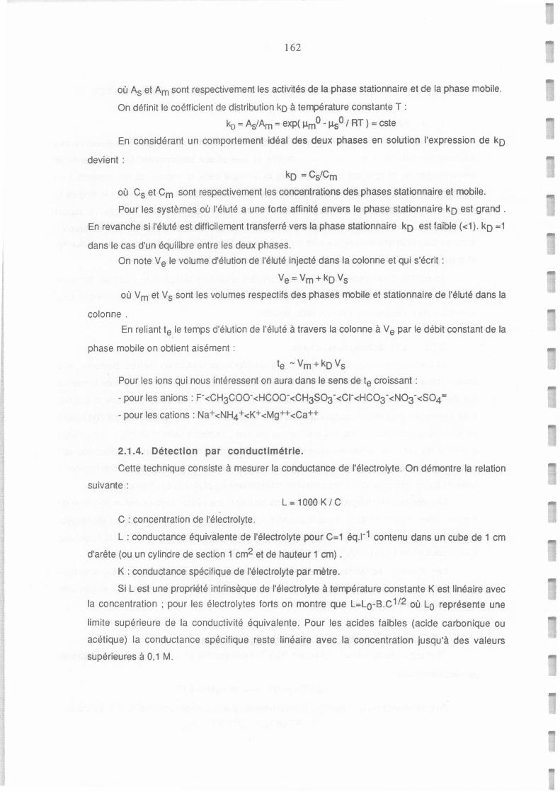
162
où As et Am sont respectivement les activités de la phase stationnaire et de la phase mobile.
On définit le coéfficient de distribution ko à température constante T :
k0 =As/Am= exp{ ~0- ~O / RT) = este
En considérant un comportement idéal des deux phases en solution l'expression de ko
devient :
ko = Cs/Cm
où Cs et Cm sont respectivement les concentrations des phases stationnaire et mobile.
Pour les systèmes où l'éluté a une forte affinité envers le phase stationnaire ko est grand .
En revanche si l'éluté est difficilement transferré vers la phase stationnaire ko est faible {<1). ko =1
dans le cas d'un équilibre entre les deux phases.
On note Ve le volume d'élution de l'éluté injecté dans la colonne et qui s'écrit :
Ve= Vm+ko Vs
où Vm et Vs sont les volumes respectifs des phases mobile et stationnaire de l'éluté dans la
colonne .
En reliant te le temps d'élution de l'éluté à travers la colonne à Ve par le débit constant de la
phase mobile on obtient aisément :
te -Vm+ko Vs
Pour les ions qui nous intéressent on aura dans le sens de te croissant :
- pour les anions: F-<CH3COO-<HCOO-<CH3SO3-<Cl-<HCO3-<NO3-<SO4=
- pour les cations : Na+ <NH4 + <K+ <Mg++ <Ca++
2.1.4. Détection par conductlmétrle.
Cette technique consiste à mesurer la conductance de l'électrolyte. On démontre la relation
suivante:
L = 1000 K / C
C : concentration de l'électrolyte.
L : conductance équivalente de l'électrolyte pour C=1 éq.I-1 contenu dans un cube de 1 cm
d'arête {ou un cylindre de section 1 cm2 et de hauteur 1 cm) .
K : conductance spécifique de l'électrolyte par mètre.
Si L est une propriété intrinsèque de l'électrolyte à température constante K est linéaire avec
la concentration ; pour les électrolytes forts on montre que L=Lo-B.C 1 /2 où Lo représente une
limite supérieure de la conductivité équivalente. Pour les acides faibles {acide carbonique ou
acétique) la conductance spécifique reste linéaire avec la concentration jusqu'à des valeurs
supérieures à 0, 1 M.
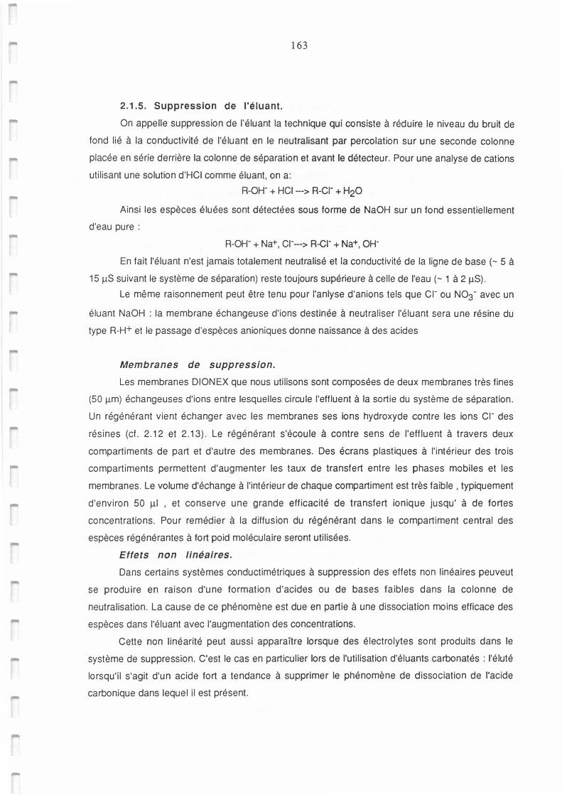
163
2.1.5. Suppression de l'éluant.
On appelle suppression de l'éluant la technique qui consiste à réduire le niveau du bruit de
fond lié à la conductivité de l'éluant en le neutralisant par percolation sur une seconde colonne
placée en série derrière la colonne de séparation et avant le détecteur. Pour une analyse de cations
utilisant une solution d'HCI comme éluant, on a:
R-oH- + HCI --> R-cI- + H2O
Ainsi les espèces éluées sont détectées sous forme de NaOH sur un fond essentiellement
d'eau pure :
R-oH- + Na+, ci---> R-eI- + Na+, OH-
En fait l'éluant n'est jamais totalement neutralisé et la conductivité de la ligne de base (- 5 à
15 µS suivant le système de séparation) reste toujours supérieure à celle de l'eau (- 1 à 2 µS).
Le même raisonnement peut être tenu pour l'anlyse d'anions tels que ci- ou No3- avec un
éluant NaOH : la membrane échangeuse d'ions destinée à neutraliser l'éluant sera une résine du
type R-H+ et le passage d'espèces anioniques donne naissance à des acides
Membranes de suppression.
Les membranes DIONEX que nous utilisons sont composées de deux membranes très fines
(50 µm) échangeuses d'ions entre lesquelles circule l'effluent à la sortie du système de séparation.
Un régénérant vient échanger avec les membranes ses ions hydroxyde contre les ions ci- des
résines (cf . 2.12 et 2.13) . Le régénérant s'écoule à contre sens de l'effluent à travers deux
compartiments de part et d'autre des membranes. Des écrans plastiques à l'intérieur des trois
compartiments permettent d'augmenter les taux de transfert entre les phases mobiles et les
membranes. Le volume d'échange à l'intérieur de chaque compartiment est très faible , typiquement
d'environ 50 µI , et conserve une grande efficacité de transfert ionique jusqu' à de fortes
concentrations . Pour remédier à la diffusion du régénérant dans le compartiment central des
espèces régénérantes à fort poid moléculaire seront utilisées.
Effets non linéaires.
Dans certains systèmes conductimétriques à suppression des effets non linéaires peuveut
se produire en raison d'une formation d'acides ou de bases faibles dans la colonne de
neutralisation. La cause de ce phénomène est due en partie à une dissociation moins efficace des
espèces dans l'éluant avec l'augmentation des concentrations.
Cette non linéarité peut aussi apparaître lorsque des électrolytes sont produits dans le
système de suppression. C'est le cas en particulier lors de l'utilisation d'éluants carbonatés : l'éluté
lorsqu'il s'agit d'un acide fort a tendance à supprimer le phénomène de dissociation de l'acide
carbonique dans lequel il est présent.
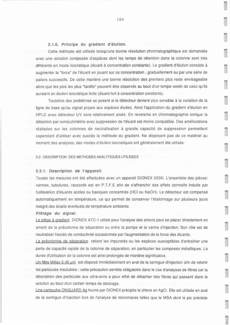
164
2.1.6. Principe du gradient d'élutlon.
Cette méthode est utilisée lorsqu'une bonne résolution chromatographique est demandée
avec une solution composée d'espèces dont les temps de rétention dans la colonne sont très
différents en mode isocratique (éluant à concentration constante). Le gradient d'élution consiste à
augmenter la "force" de l'éluant en jouant sur sa concentration , graduellement ou par une série de
paliers successifs . De cette manière une bonne résolution des premiers pics reste envisageable
alors que les pics les plus "tardifs" peuvent être observés au bout d'un temps voisin de celui qu'ils
auraient en élution isocratique forte (éluant fort à concentration constante).
Toutefois des problèmes se posent si le détecteur devient plus sensible à la variation de la
ligne de base qu'au signal propre aux espèces éluées. Ainsi l'application du gradient d'élution en
HPLC avec détecteur UV sera relativement aisée. En revanche en chromatographie ionique la
détection par conductimétrie avec suppression de l'éluant est moins compatible. Des améliorations
réalisées sur les colonnes de neutralisation à grande capacité de suppression permettent
cependant d'utiliser avec succès la méthode du gradient. Ne disposant pas de ce matériel au
moment des analyses, des modes d'élution isocratiques ont généralement été utilisés.
2.2 : DESCRIPTION DES METHODES ANALYTIQUES UTILISEES
2.2.1. Description de l'appareil.
Toutes les mesures ont été effectuées avec un appareil DIONEX 2000i. L'ensemble des pièces:
vannes, tubulures , raccords est en P.T.F.E afin de s'affranchir des effets corrosifs induits par
l'utilisatiion d'éluants acides ou basiques concentrés (HCI ou NaOH). Le détecteur est compensé
automatiquement en température, ce qui permet de conserver l'étalonnage sur plusieurs jours
malgré des écarts éventuels de température ambiante.
Filtrage du signal.
Le piège à gradient DIONEX ATC-1 utilisé pour l'analyse des anions peut se placer directement en
amont de la précolonne de séparation ou entre la pompe et la vanne d'injection. Son rôle est de
neutraliser l'excès de conductivité occasionnée par l'augmentation de la force des éluants.
La précolonne de séparation retient les impuretés ou les espèces susceptibles d'entraîner une
perte de capacité rapide de la colonne de séparation, en particulier les composés métalliques. La
durée d'utilisation de la colonne est ainsi prolongée de manière significative.
Un filtre Millex 0,45 um est disposé immédiatement en aval de la seringue d'injection afin de retenir
les particules insolubles : cette précaution semble obligatoire dans le cas d'analyses de filtres car la
désorption des particules aux ultra-sons a pour effet de détacher des fibres qui passent dans la
solution au bout d'un certain temps de stockage.
Une cartouche ONGUARD Ag founie par DIONEX précipite le chlore en AgCI. Elle est utilisée en aval
de la seringue d'injection lors de l'analyse de microtraces telles que le MSA dont le pic précède
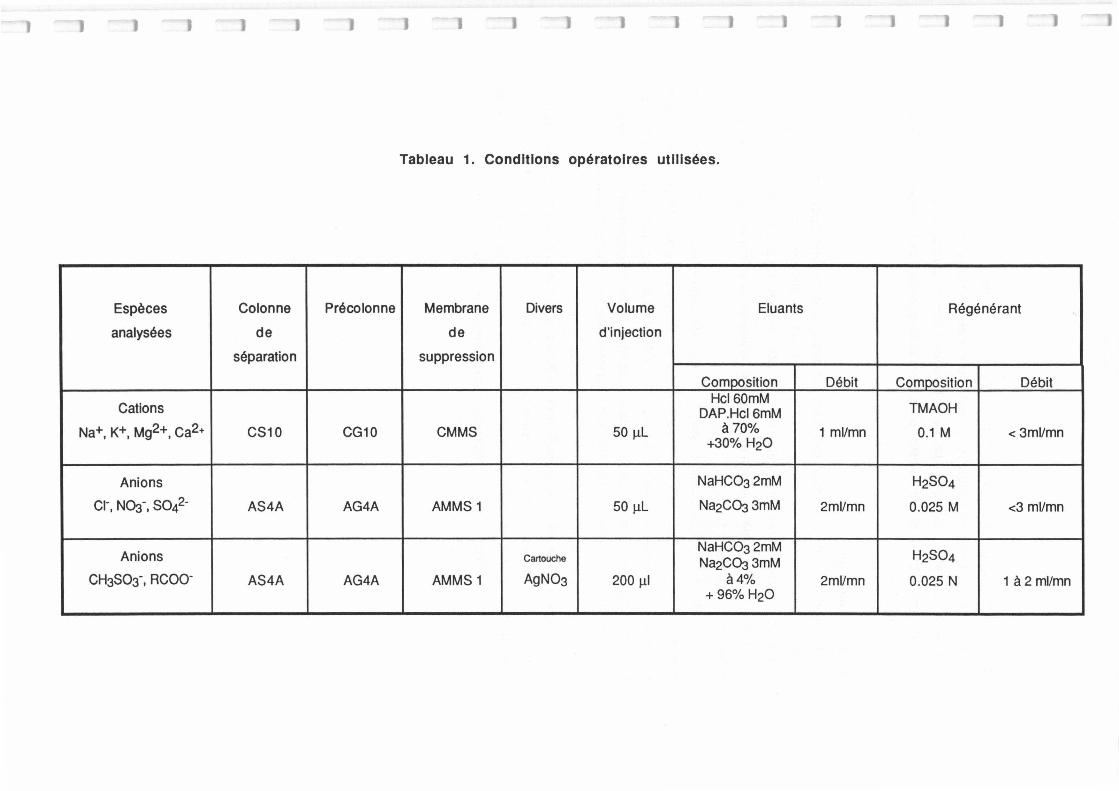
Tableau 1. Conditions opératoires utlllsées.
Espèces Colonne Précolonne Membrane Divers Volume Eluants Régénérant
analysées de de d'injection
séparation suppression
Comoosition Débit Composition Débit
Cations Hel 60mM
TMAOH DAP.Hcl 6mM Na+, K+, Mg2+, Ca2+ CS10 CG10 CMMS 50 µL à70%
+30% H2O 1 ml/mn 0.1 M <3ml/mn
Anions NaHCO32mM H2SO4
c1- NO:f SO 2· 1 1 4 AS4A AG4A AMMS1 50 µL Na2CO33mM 2ml/mn 0.025 M <3 ml/mn
Anions NaHCO32mM
H2SO4 Canouche Na2CO33mM CH3SO3·, RCoo- AS4A AG4A AMMS1 AgNO3 200 µI à4% 2ml/mn 0.025 N 1 à 2 ml/mn
+ 96% H2O
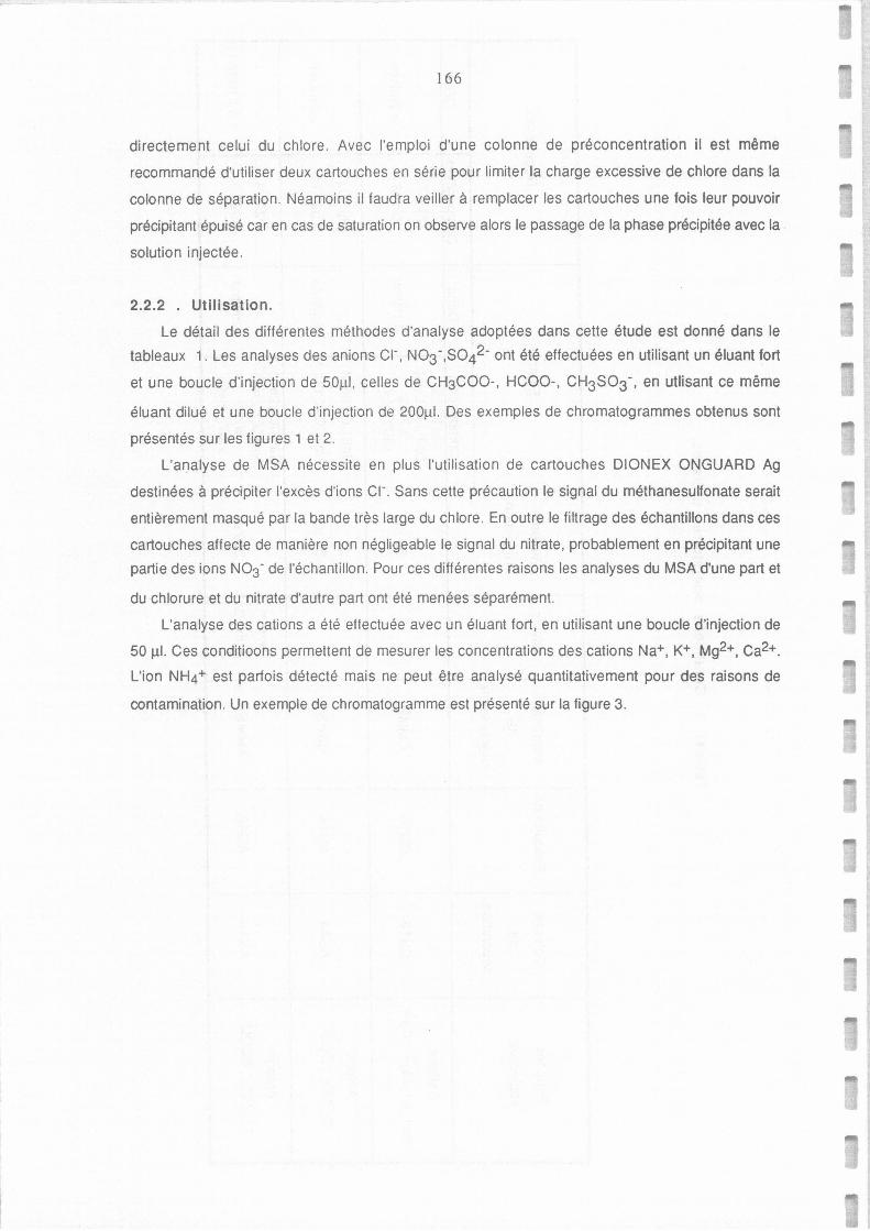
166
directement celui du chlore. Avec l'emploi d'une colonne de préconcentration il est même
recommandé d'utiliser deux cartouches en série pour limiter la charge excessive de chlore dans la
colonne de séparation. Néamoins il faudra veiller à remplacer les cartouches une fois leur pouvoir
précipitant épuisé car en cas de saturation on observe alors le passage de la phase précipitée avec la
solution injectée .
2.2.2 . Utilisation.
Le détail des différentes méthodes d'analyse adoptées dans cette étude est donné dans le
tableaux 1. Les analyses des anions cr, No3-,sol- ont été effectuées en utilisant un éluant fort
et une boucle d'injection de 50µ1, celles de CH3COO-, HCOO-, CH3S03-, en utlisant ce même
éluant dilué et une boucle d'injection de 200µ1. Des exemples de chromatogrammes obtenus sont
présentés sur les figures 1 et 2.
L'analyse de MSA nécessite en plus l'utilisation de cartouches DIONEX ONGUARD Ag
destinées à précipiter l'excès d'ions ci- . Sans cette précaution le signal du méthanesulfonate serait
entièrement masqué par la bande très large du chlore . En outre le filtrage des échantillons dans ces
cartouches affecte de manière non négligeable le signal du nitrate, probablement en précipitant une
partie des ions No3- de l'échantillon. Pour ces différentes raisons les analyses du MSA d'une part et
du chlorure et du nitrate d'autre part ont été menées séparément.
L'analyse des cations a été effectuée avec un éluant fort, en utilisant une boucle d'injection de
50 µI. Ces conditioons permettent de mesurer les concentrations des cations Na+, K+, Mg2+, Ca2+.
L'ion NH4+ est parfois détecté mais ne peut être analysé quantitativement pour des raisons de
contamination. Un exemple de chromatogramme est présenté sur la figure 3.
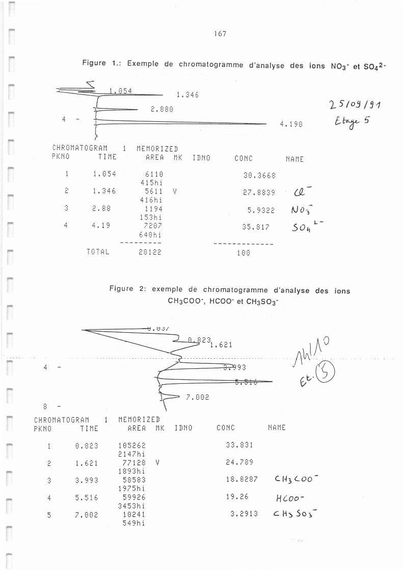
4
8
167
Figure 1.: Exemple de chromatogramme d 'analyse des ions N03· et S04
2-
1. 054
4 4. 1 90
CH RO t·1 AT O Ci F.: A t·1 t·1Et·10F.: I ZED F'Kt-JO
2
., 't
T H1E
1. i:::i 5 4
1 .:346
4. 1 13
TOTAL
AF.:EA t·1K IDt·lO
61 Hl 415hi
5E, 11 V
1 i '3 4 153hi
72(17
2(1 î 22
COt·iC t-Jf:H-1[
5.'3322
.s O '1 1..-
1 G i:)
Figure 2 : exemple de chromatogramme d 'analyse des ions
CH3Coo-, Hcoo- et CH3S03·
:_ • 1:1.5/
7. l:1[12
CHROt-1ATOCiRAt-1 t-JEt·10RIZED PUJO TI t·1E
.-, C
·:i ·-·
4
C" ·-'
1;:,. 823
1 . 6 21
5.516
7.E102
AF.:EA tff I Dt-iO
105262 2147hi
7712B V 18'3:3h i
58583 1975hi
5'3'32E1
345:3h i 11:)241 549hi
COMC t-HH1E
24. 78'3
18.8287 C.H~l.DO-
1 '3. 26
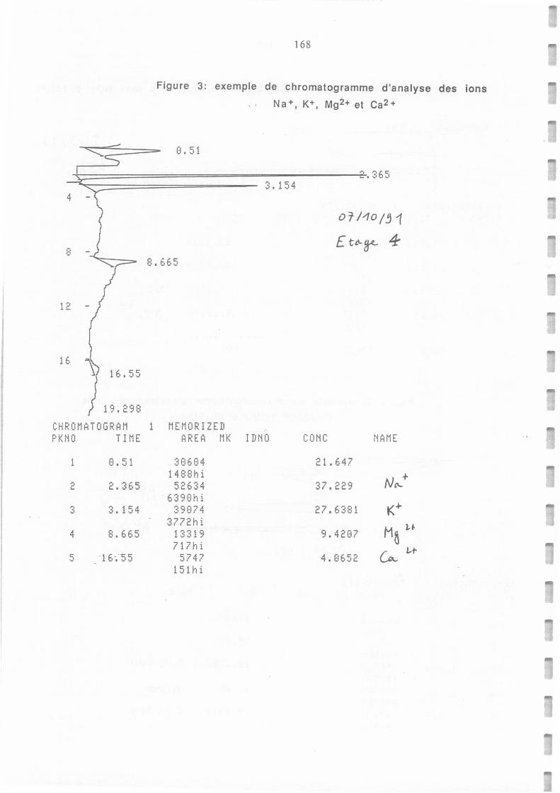
8
1 .-. C.
16 16.55
1'3.2'3B
168
Figure 3: exemple de chromatogramme d'analyse des ions
Na+, K+, Mg 2+ et Ca 2 +
CHROMATOGRAM 1 MEMORIZED PKNO TIME AREA MK IDNO CONC MAt1E
1 0. 51 3E16134 21.647 1488hi
.-. ·=· 365 52E,~:4 C. L.. ~:7.229 6391:ih i
-:, ~· r, .:,1 • 154 ~:9074 27.6~:81
~:772h i 4 8. E.E,5 1~:~:19 9.42137
717hi C"
·-' -1e.-.-·55 5747 4. tl652 151hi
169
Annexe III
Méthode de mesure de la
concentration de noyaux d' Aïtken

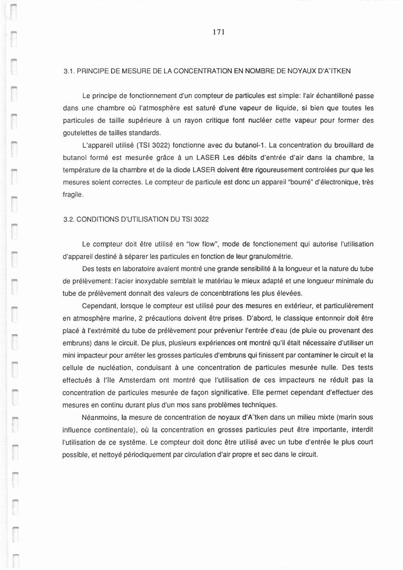
171
3.1 . PRINCIPE DE MESURE DE LA CONCENTRATION EN NOMBRE DE NOYAUX D'A""ITKEN
Le principe de fonctionnement d'un compteur de particules est simple: l'air échantilloné passe
dans une chambre où l'atmosphère est saturé d 'une vapeur de liquide, si bien que toutes les
particules de taille supérieure à un rayon critique font nucléer cette vapeur pour former des
goutelettes de tailles standards.
L'appareil utilisé (TSI 3022) fonctionne avec du butanol-1. La concentration du brouillard de
butanol formé est mesurée grâce à un LASER Les débits d 'entrée d'air dans la chambre , la
température de la chambre et de la diode LASER doivent être rigoureusement controlées pur que les
mesures soient correctes . Le compteur de particule est donc un appareil "bourré" d'électronique, très
fragile .
3.2. CONDITIONS D'UTILISATION DU TSI 3022
Le compteur doit être utilisé en "low flow", mode de fonctionement qui autorise l'uti lisation
d'appareil destiné à séparer les particules en fonction de leur granulométrie.
Des tests en laboratoire avaient montré une grande sensibilité à la longueur et la nature du tube
de prélèvement: l'acier inoxydable semblait le matériau le mieux adapté et une longueur minimale du
tube de prélèvement donnait des valeurs de concenbtrations les plus élevées.
Cependant , lorsque le compteur est utilisé pour des mesures en extérieur, et particulièrement
en atmosphère marine, 2 précautions doivent être prises. D'abord, le classique entonnoir doit être
placé à l'extrémité du tube de prélèvement pour préveniur l'entrée d'eau (de pluie ou provenant des
embruns) dans le circuit. De plus, plusieurs expériences ont montré qu'il était nécessaire d'utiliser un
mini impacteur pour arréter les grosses particules d'embruns qui finissent par contaminer le circuit et la
cellule de nucléation, conduisant à une concentration de particules mesurée nulle. Des tests
effectués à l'île Amsterdam ont montré que l'utilisation de ces impacteurs ne réduit pas la
concentration de particules mesurée de façon significative. Elle permet cependant d'effectuer des
mesures en continu durant plus d'un mos sans problèmes techniques.
Néanmoins, la mesure de concentration de noyaux d'A"tken dans un milieu mixte (marin sous
influence continentale), où la concentration en grosses particules peut être importante, interdit
l'utilisation de ce systême. Le compteur doit donc être utilisé avec un tube d'entrée le plus court
possible , et nettoyé périodiquement par circulation d'air propre et sec dans le circuit.
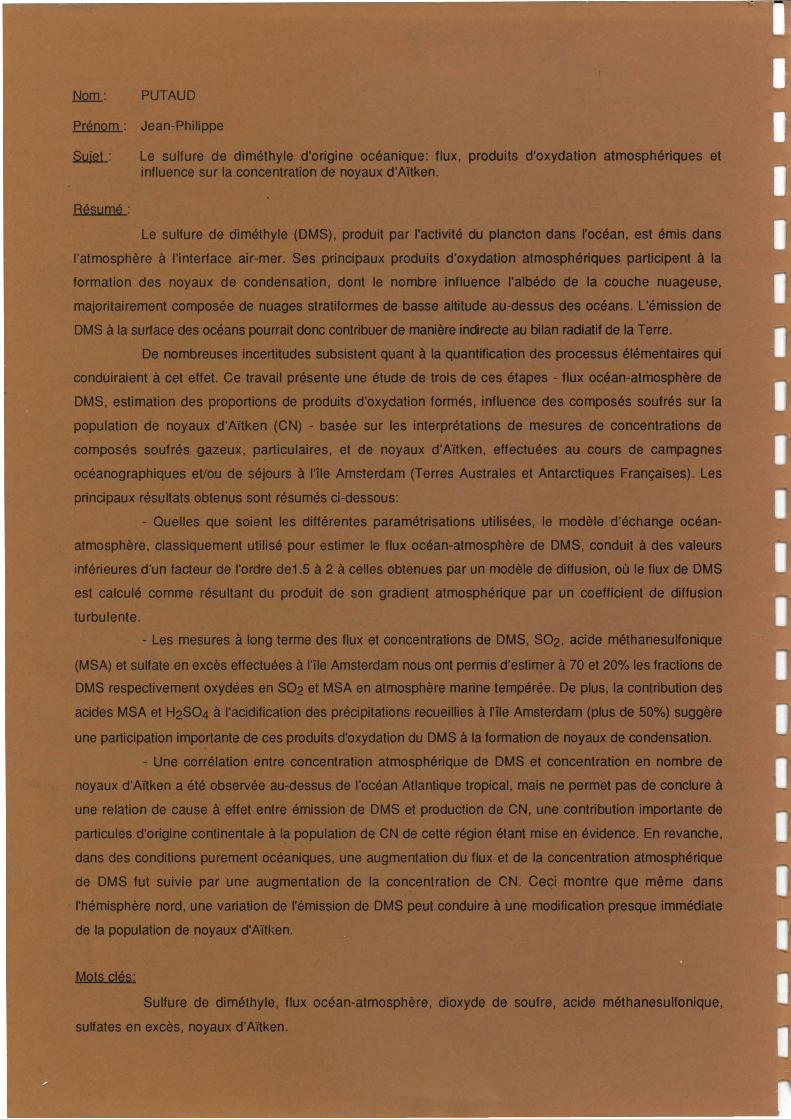
~: PUTAUD
prénom : Jean-Philppe
~: Le sulfure de dlméthyle d~ne océanique: flux, produits d'oxyctatiOn atmosphériques et influence sur la concentration de noyaux d'A11ken.
Résumé: Le sulfure de dfméthyle (OMS), produil par ractlvlté du pl&P,d,Q_Q ._ roçéan, est émis dans
l'atmosphère à l'int~rface aiNner. ses &>,jndpaux prodUit8 d'oxy_.,,n ~ participent à la
formation des noyaux de condensalton, dent te nombre lnfhAence ,...,...._ la 'couche nuageuse,
majoritairement. ~le de nuages atratiformes de base allltudl ...._. oœana. L'émssion de
OMS à la SUl'face dl8 006.ans.~ donc èCJlllrlbUerde manlêre inclrecle au bilan__. de la Terre.
De nD8lbrauses ~ Sùbl'atent quant à la~ ÎIS ~· élémerhires qui
conduiraient à cet effet. Ce travail """11• une étude4t trois de ces 6tapls - llûx oc:fan-atmosphère de
OMS, estimation des proportlOns de prodUits dtoxydatk>n fOtmés, iJttluetlCe dèJ ~és soufrés sur la
population de noyaux d' Altken (CN) - baNe sur les lnteg,rétatlona de mesures de concentrations de
composés souft 14%eux, partfcutlll'es, et de aoyaU)( d'A1tken, effeclUéet -~ de campagnes
océanographiques eC/Qù ~ silot,lrs à me Amsterdam (Terres Australes et Ani .. ~es). Les
prlncipaux-'fésulats ôbterur .-rfsumés cl~:
- Quelle& qu• _,,.,_ f8s 'dllMtentes paramétrisallons utilsée&, lë ~ d'éOl.lange océan-
atmosphère, ~ utilJNi)OUr ..,_ te fltx ocfan-atmospJtère dé DM&. .,.,.. à *6 valeurs
Inférieures crun tacla df roRte de1 .5 à z à èelles Obit,_. par un modtle de cft"'*'1J oè te flux de DMS
est calculé comme rlMUltant dU f)n)dUlt • _,n o,adient atmosphéttque pat, ua ~- de clffusion
de la population de noyaux ctAJ{lçen.
Sulftn de cltbê1b;Je. fJUX océan-atmospbtfe:; drOxydlt de aoufœ, «cide mêttlanesulfOnlque,
sulfates en excès. noyaux -d'AltheJI.


